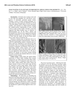
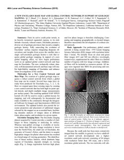
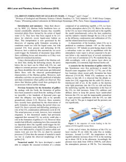
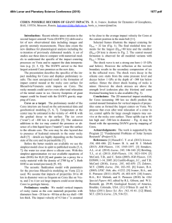
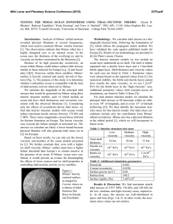
46th Lunar and Planetary Science Conference (2015) 1124.pdf TOPOGRAPHIC ANALYSIS OF SAMARIA FOSSA ON ENCELADUS: THERMAL GRADIENT, HEAT FLUX, AND POSSIBLE STRESS SOURCES DETERMINED FROM NORMAL FAULTING Amanda L. Nahm1 and Simon A. Kattenhorn2, 1Department of Geological Sciences, University of Idaho, Moscow, ID 83844, [email protected], 2ConocoPhillips Company, 600 N. Dairy Ashford, Houston, TX 77079, [email protected]. Introduction: Tectonic features on Enceladus and other outer solar system bodies provide a framework for interpreting their linked geologic, tectonic, and orbital histories. On Europa [1], Ganymede [2], Dione [3], Tethys [4], and elsewhere on Enceladus [5], normal fault topography has been used to infer properties of the lithosphere as well as the heat flux at the time of fault formation. We identify a NNE-striking normal fault on Enceladus in the northern trailing hemisphere, recently named Samaria Fossa (Fig. 1), with a length of ~195 km and a maximum relief of ~570 m. Samaria Fossa (SF) crosscuts all troughs and craters and, with one notable exception in the south, is not cut by craters larger than the available image resolution. Therefore, SF is likely young relative to its surroundings. Estimates of brittle lithosphere thickness derived from SF, coupled with lithospheric strength envelopes appropriate for ice, allow for the determination of thermal gradients in the ice during its formation. In addition, stresses required for its formation are calculated, which will place bounds on possible formation mechanisms and sources of stress. graphic profiles (40 km long) were taken ~10 km from the fault center. The profile sets were stacked and averaged to obtain the mean topography. A regional slope (~0.3º) was removed from the topographic profiles (i.e., the profiles were detrended) prior to mechanical modeling (Fig. 2). Mechanical Modeling: To determine Samaria Fossa’s dip angle, depth of faulting, and accumulated displacement, we perform forward modeling of faultrelated topography [e.g., 8, 9] using the forward mechanical dislocation modeling program Coulomb* [10, 11]. This approach has been shown to provide remarkably good fits to the observed structural topography above a fault for a relatively narrow range of parameters [e.g., 8. 9]. In general, correspondence between the output model displacements and topography suggest that the fault parameters obtained from modeling are representative of the characteristics of the modeled fault [e.g., 9, 12]. Figure 2. Averaged and detrended topographic profiles. Profile A is offset vertically by 375 m for clarity. Figure 1. Portion of Cassini Imaging Science Subsystem (ISS) global mosaic (left) and stereo-derived topography (right). Simple cylindrical projection, centered at 31.1ºN, 136ºE. Data: Topographic profiles were derived from a portion of a digital elevation model (DEM) (~150 m/px horizontal resolution), produced using Cassini ISS stereo image analysis, shape-from-shading (photoclinometry), and stereo-controlled DEMs [e.g., 6, 7]. For mechanical modeling, multiple profiles were stacked and averaged to produce a mean cumulative profile (Profile A and Profile B). For profile A, eight topographic profiles (55 km long) were taken ~30 km from the fault center and for profile B, seven topo- Stress and material displacement calculations are made in an elastic half-space with uniform isotropic properties following the equations derived by [13]. In these models, a fault is idealized as a rectangular plane with a specified sense of slip, magnitude of average displacement, fault dip angle, depth of faulting, and fault length. Results: Based on the modeling, the displacement is 520–730 m, the depth of faulting is 6.4–7.5 km (~the inferred depth of the brittle-ductile transition [BDT]), and the fault dip angle is 75º. Thermal Gradient and Heat Flux: Strength envelopes compare frictional strength, which increases linearly with depth, and creep strength, which decreases exponentially with depth for a given strain rate [e.g., 14]. The strength of the ice lithosphere is 46th Lunar and Planetary Science Conference (2015) thus defined based on two constitutive equations: one for the brittle behavior near the surface and one for the ductile deformation deeper within the ice shell. The ductile strain rate is calculated using the general form of the ductile deformation equation, known as Dorn’s equation [15-17]: " −Q % n (1) i '' ε!i = Aiσ ( z ) i d − pi exp $$ RT z ( ) # & where d is the grain size, σ(z) is the differential stress at depth z, R is the universal gas constant, T(z) is the temperature at depth, and Q is the activation energy. Ai, Qi, ni, and pi are parameters dependent on the deformation mechanism (e.g., grain boundary sliding). Thermal gradients can be derived directly from strength envelopes as defined in (1). The equation for the temperature at depth T(z) is a function of the surface temperature Ts and the thermal gradient, dT/dz: T (z) = Ts + dT z dz (2) The thermal gradient was varied until the brittleductile transition (BDT) was approximately the depth of faulting determined from forward mechanical modeling (6.4–7.5 km). The heat flux, F, is a function of the thermal conductivity of ice and the thermal gradient, determined above. The 1D relationship for conductive heat transport is known as Fourier’s law [e.g., 18] and is given by F = −k dT dz (3) where k is the temperature dependent coefficient of thermal conductivity of ice [19]. For T = Ts = 65 K, k is 7.978 W m-1 K-1. Results: Yield strength envelope calculations limit the conductive thermal gradients at this location on Enceladus to be between 8.5 and 22.3 K/km and heat fluxes between 67.8 to 177.9 mW/m2 at the time of the formation of Samaria Fossa. Stresses Required for SF Formation: In order to investigate which stress mechanisms may have been responsible for the formation of Samaria Fossa, we calculate the required cumulative driving stress for its formation following the procedure laid out in [20, 21] and summarized here. The incremental driving stress (i.e., stress drop), σd, for one fault slip event (i.e., one ice quake along the growing fault) is given by [21]: γ E σ d = quake 2 2C(1− ν ) (4) where γquake is the displacement-length ratio for one slip event (10-5–10-6 on terrestrial bodies [e.g., 22]), E is the Young’s modulus of the fractured ice at the surface (in the range 1 GPa [2, 4, 5, 23] to 9 GPa [3, 24, 25]), C is the effective driving stress factor which 1124.pdf varies between 0.4 and 0.6 [21], and ν is the Poisson’s ratio. Results: Minimum stresses required for one quake range from 0.9 (γquake = 10-6, C = 0.6, E = 1 GPa) to 126 kPa (γquake = 10-5, C = 0.4, E = 9 GPa). Discussion: The inferred BDT implies that the ice is brittle down to at least 7.4 km and ductile ice extends below that. The inferred heat flux is similar to other values inferred outside of the south polar terrain, which range from 150–270 mW/m2 [5, 25]. Averaging the thermal emission (~5.8 GW) over the entire south polar terrain gives an average heat flux of 55–110 mW/m2 [28]. Thus, our results reinforce the need for an endogenic heat source [28] other than radiogenic heating to account for the calculated and observed heat fluxes. The magnitude of diurnal tidal stresses at the surface varies over Enceladus’s 1.37-day orbit and reaches a maximum of 100 kPa [29]. Stresses of ~70 kPa may only be required for fault failure [e.g., 30]. However, whether a fault slips is not only a function of the stress magnitudes, but also on the interplay between the driving stresses (shear stresses) and the resisting stresses (normal stress and friction along the fault) resolved on the fault plane, known as the Coulomb criterion [31]. These stresses will be compared to stresses calculated using SatStressGUI [32] and evaluated with the Coulomb criterion to evaluate whether diurnal stresses are sufficient to cause slip at depth on Samaria Fossa. * Available at http://earthquake.usgs.gov/research/software/coulomb/ References: [1] Nimmo, F. and P. Schenk (2006), JSG, 28, 2194–2203; [2] Nimmo et al. (2002), GRL, 29, 1158; [3] Hammond, N. P., et al. (2013), Icarus, 233, 418–422; [4] Giese, B., et al. (2007), GRL, 34, L21203; [5] Giese, B., et al. (2008), GRL, 35, L24204; [6] Schenk, P. M. (2002), Nature, 417, 419–421. [7] Schenk, P. M. and R. T. Pappalardo (2004), GRL, 31, L16703; [8] Cohen, S.C. (1999), Advanced Geophys., 41, 133–231. [9] Schultz, R. A. and J. Lin (2001), JGR, 106, 16549–16566; [10] Lin, J. and R. S. Stein (2004), JGR, 109, B02303; [11] Toda, S., et al. (2005), JGR, 110, B05S16; [12] Nahm, A. L., et al. (2013), JGR-Planets, 118, 190–205; [13] Okada, Y. (1992), BSSA, 82, 1018–1040. [14] Ranalli, G. (1997), in Orogeny through time, J.-P. Burg and M. Ford (eds.), Geol. Soc. Sp. Pub. 121, pp. 19–37; [15] Ranalli, G. (1995), Rheology of the Earth, 2nd ed., Chapman and Hall, London; [16] Durham, W. B., et al. (1997), JGR, 102, 16293– 16302; [17] Goldsby, D. L., and D. L. Kohlstedt (2001), JGR, 106, 11017– 11030. [18] Turcotte, D. L. and G. Schubert (2002), Geodynamics, 2nd ed., Cambridge Univ. Press, Cambridge, U.K.; [19] Hobbs, P. V. (1974), Ice Physics, Clarendon Press, Oxford; [20] Nahm, A. L. and R. A. Schultz (2013), in Volcanism and Tectonism Across the Inner Solar System, Platz, T., Massironi, M., Byrne, P. K. & Hiesinger, H. (eds), Geol. Soc. Sp. Pub.; [21] Schultz, R. A. (2003), GRL, 30, 1593; [22] Scholz, C.H. (1997), Geowissenschaften, 15, 124–130. [23] Vaughan, D. G. (1995), JGR, 100, 6213–6224; [24] Gammon, P. H., et al. (1983), J. Phys. Chem., 87, 4025– 4029; [25] Bland, M. T., et al. (2012), GRL, 39, L17204; [26] Cowie, P.A. and Scholz, C.H. (1992), JSG, 14, 1133–1148; [27] Spencer et al. (2006), Science, 311, 1401–1405; [28] Spencer et al. (2009), in Saturn from CassiniHuygens, M. K. Dougherty et al. (eds.), pp. 683–724; [29] Hurford et al. (2007), Nature, 447, 292-294; [30] Smith-Konter and Pappalardo (2008), Icarus, 198, 435–451; [31] Byerlee, J. D. (1978), Pure Appl. Geophys. 116, 615–626; [32] Kay, J. P. and S. A. Kattenhorn (2010), LPSC 41, abstract #2046.