Download Report

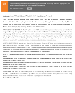
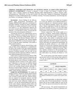
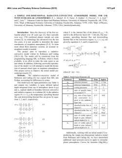
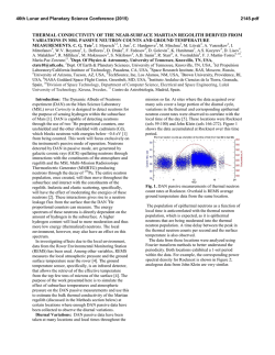
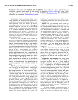
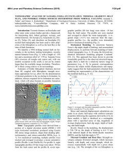
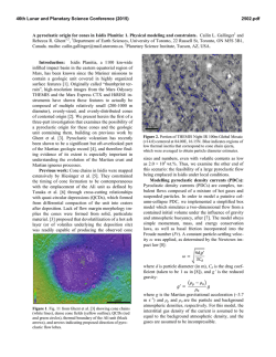
46th Lunar and Planetary Science Conference (2015)
1093.pdf
ONE-DIMENSIONAL THERMAL CONVECTION CALCULATION USING A MODIFIED MIXING
LENGTH THEORY. S. Kamata1,2*, F. Nimmo1, and K. Kuramoto2 1Dept. Earth and Planetary Sciences, University
of California Santa Cruz, 1156 High St, Santa Cruz, CA 95064, USA, 2Dept. Natural History Sciences, Hokkaido
University, Kita-10 Nishi-8, Kita-ku, Sapporo, Hokkaido 060-0810, Japan (*[email protected]).
Summary: We develop a one-dimensional scaling
based on mixing length theory and compare with 3D
calculation results. We find that the mean temperature
(m) and Nusselt number (Nu) are overestimated and
underestimated, respectively, when we use a conventional definition of the mixing length (l). We calculate
m and Nu varying the definition of l under a wide variety of parameter conditions and derive a set of simple
formulae for l that produces accurate values of m and
Nu under steady-state isoviscous cases.
Introduction: Thermal convection is considered to
play a major role in the thermal evolution of planetary
bodies since it can transport heat more efficiently than
thermal conduction. A major issue for convection calculations is the high computational cost. Although
computational speed has been greatly increased recently, parameterized convection codes are still applied to
parameter studies [e.g., 1].
Parameterized convection is a box model using a
scaling law for Nusselt number (Nu) and Rayleigh
number (Ra) determined based on 3D calculations [e.g.,
2]. Because this is a box model, a single representative
value of physical properties needs to be specified to
calculate Ra. Nevertheless, physical properties may
vary largely with depth in the convective region, and it
may be difficult to choose an appropriate value.
A one-dimensional thermal convection calculation
using mixing length theory (MLT) is free from such a
problem. In this scheme, convective heat transport is
expressed by, adding to the usual conduction equation,
a term that appears when the thermal gradient exceeds
the adiabatic gradient:
𝑑𝑇
1 𝑑
𝑑𝑇
𝑑𝑇 𝑑𝑇
𝜌𝐶
= 2 [𝑟 2 𝑘
+ 𝑟 2 𝑘𝑣 ( − | )] + 𝜌𝑄
𝑑𝑡
𝑟 𝑑𝑟
𝑑𝑟
𝑑𝑟 𝑑𝑟 𝑎
where  is density, C is specific heat, T is temperature,
t is time, r is radial distance from the center, k is thermal conductivity, kv is effective thermal conductivity
due to convection, Q is volumetric heating rate, and
(dT/dr|a) is the adiabatic thermal gradient, respectively
[e.g., 3]. The effective thermal conductivity kv depends
on the mixing length l, which is usually assumed to be
the distance to the nearest boundary (upper or lower
boundary) of the convective region.
The major advantage of MLT is its low calculation
cost; because this is a one-dimensional scheme, the
calculation cost is almost the same as that of conduction calculation. Another advantage is that all the parameters can be determined locally; this scheme can be
easily applied to a case whose physical properties of
the convective region vary significantly with depth.
Consequently, the MLT scheme is suitable to apply
parameter studies for thermal evolution of planetary
bodies and has been applied to the early Earth [e.g., 3],
early Mars [4], icy satellites [5], and super-Earths [6].
It has been shown that this scheme can well reproduce the Nu~Ra1/3 relation for an isoviscous, bottom
heated case even though this scheme does not require
Ra-Nu scaling laws [3]. However, a detailed comparison with recent 3D calculation results has not been
conducted yet. In this study, we calculate the nondimensional mean temperature (m) and Nusselt number (Nu) under a wide variety of parameter conditions
(i.e., Ra, curvature, and heat production rate), and
compare with 3D calculation results [7]. We conduct
examinations for bottom heated and mixed heating
cases separately because scaling laws for m and for Nu
are different between these cases.
Mixing Length: Figure 1 shows l as a function of
depth schematically. In order to minimize the number
of free parameters, we assume that l = 0 at the upper
and lower boundaries under all conditions and vary (1)
the peak depth aH where l has the maximum value and
(2) the maximum value bH of l. Here, H is the thickness of the convective region. We assume that l increases and decreases linearly with depth below and
above z = aH, respectively. Previous studies define l as
the distance to the nearest boundary: a = b = 0.5.
Bottom Heated Case: Figure 2 shows m as a
function of f, the ratio of the bottom radius to the upper
radius; f = 0 and 1 indicates that the convective region
Figure 1: The mixing length (l) as a function of depth (z). H
is the thickness of the convective region. Free parameters are
a (the peak depth) and b (the maximum value).
46th Lunar and Planetary Science Conference (2015)
Figure 2: The mean temperature m as a function of f for
bottom heated cases. Cross symbols and circles show results
for the conventional (original) MLT (a = b = 0.5) and those
for the adjusted MLT, respectively.
is a sphere and a plane, respectively. For all f, the conventional MLT using a = b = 0.5 overestimates m, and
the difference can be up to ~0.1. We also found that
the conventional MLT underestimates Nu under all
calculation conditions and that the relative error can be
up to >60%. In order to obtain a set of simple formulae
for a and b that leads to m and Nu close to those of 3D
results, we calculated m and Nu varying values of a
and b and then calculated the root mean square error of
prediction (RMSEP). We found that the following
equations lead to sufficiently small errors; the difference in m becomes <~0.015 (circles in Figure 2) and
the relative error of Nu becomes <~15% .
𝑎 = 𝑓(1 − 𝑓/2)
𝑏 = 1.43 × 0.696𝑓
Mixed Heating Case: A similar analysis was carried out for mixed heating cases. We found that the
conventional MLT scheme leads to errors of m and Nu
that can be up to ~100% and ~60%, respectively (Figure 3). We conducted a non-linear regression analysis
to obtain a set of simple formulae for a and b as functions of f and h. Here, h is the non-dimensional internal
heating rate defined as h = QH2/(kT) where T is
the temperature difference between the bottom and the
top of the shell. We found that
𝑎 = 0.223𝑓 + 8.01 × 10−3 ℎ + 0.325
𝑏 = −0.733𝑓 2 + 0.858𝑓 + 1.17 × 10−2 ℎ + 0.716
gives errors <~15% (Figure 3), which are much smaller than those resulting from the conventional MLT.
Discussion and Future Work: The obtained empirical equations of a and b for the bottom heated case
are different from those derived for mixed heating
conditions. This is not unexpected, since the scaling
laws based on 3D calculations between these cases are
also different [7].
1093.pdf
The actual convection occurs in 3D space, and lateral motion has a large effect on temperature near the
boundary layers; the temperature immediately below
the top (and cold) boundary layer, for example, is
higher than the mean temperature, resulting in a negative thermal gradient [8]. Such a temperature profile
cannot be reproduced as long as we use a simple definition of l (Figure 1). Nevertheless, the use of a more
complex definition of l may lose one of the major advantages of the MLT scheme that the calculation cost
is very small.
The viscosity of silicates and ices depends strongly
on temperature. For this initial study, however, we
consider only isoviscous cases. A further study considering temperature-dependent viscosity is needed.
Acknowledgments: We thank Y. Abe, J. Besserer, J.
Kimura, and T. Yanagisawa for fruitful discussions. This
work was supported by JSPS Grant-in-Aid for JSPS Fellows.
References: [1] Grott et al. (2011) EPSL, 307, 135-146.
[2] Solomatov (1995) Phys. Fluids, 7, 266-274. [3] Abe
(1995) The Earth's Central Part: Its Structure and Dynamics,
pp. 215-235. [4] Senshu et al. (2002) JGR, 107, doi:10.1029/
2001JE001819. [5] Kimura et al. (2009) Icarus, 202, 216224. [6] Tachinami et al. (2011) ApJ, 726, 70-88. [7] Deschamps et al. (2010) GJI, 182, 137-154. [8] McKenzie et al.
(1974) J. Fluid Mech., 62, 465-538.
Figure 3: The comparison of the mean temperature m ((a)
and (b)) and Nusselt number Nu ((c) and (d)) for mixed heating cases. Here, h is the non-dimensional heating rate. Errors
in m and Nu for the conventional (original) MLT are up to
~100% and ~60%, respectively. Those for the adjusted MLT
are reduced to <~15%.