Download Report

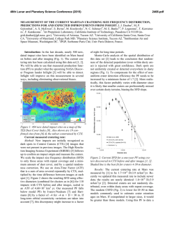
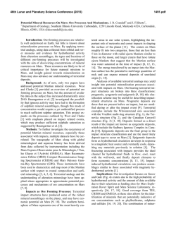
46th Lunar and Planetary Science Conference (2015)
1339.pdf
MAPPING MARS’ NORTHERN PLAINS: ORIGINS, EVOLUTION AND RESPONSE TO CLIMATE
CHANGE - AN OVERVIEW OF THE GRID MAPPING METHOD. Ramsdale, J.D.1, Balme, M.R.1,2, Conway,
S.J., Costard, F., Gallagher, C., van Gasselt, S., Hauber, E., Johnsson, A.E., Kereszturi, A., Platz, T., Séjourné, A.,
Skinner, J.A., Jr., Reiss, D., Swirad, Z., Orgel, C., Losiak, A. 1Dept. Physical Sciences, Open University, Walton
Hall, Milton Keynes, MK7 6AA ([email protected]). 2Planetary Science Institute, Suite 106, 1700 East
Fort Lowell, Tuscon, AZ, USA.
Introduction: An International Space Science
Institute (ISSI) team project has been convened to
study the northern plains of Mars. It uses
geomorphological mapping to compare ice-related
landforms in the three northern plains basins: Acidalia
Planitia, Arcadia Planitia, and Utopia Planitia. The
main science questions this project aims to answer are:
1) “What is the distribution of ice-related landforms in
the northern plains, and can it be related to distinct
latitude bands or different geological or
geomorphological units?”
2) “What is the relationship between the latitude
dependent mantle (LDM) and (i) landforms indicative
of ground ice, and (ii) other geological units in the
northern plains?”
3) “What are the distributions and associations of
recent landforms indicative of thaw of ice or snow?”
With increasing coverage of high-resolution images
of the surface of Mars (e.g. Context Imager – CTX, ~ 6
m/pixel, covering ~ 90% of the surface as of December
2014 [1]) we are able to identify increasing numbers
and varieties of small-scale landforms. Many such
landforms are too small to represent on regional maps,
yet determining their presence or absence across large
areas can form the observational basis for developing
hypotheses on the nature and history of an area. The
combination of improved spatial resolution with nearcontinuous coverage increases the time required to
analyse the data. This becomes problematic when
attempting regional or global-scale studies of metrescale landforms. Here, we describe an approach for
mapping small features across large areas that was
formulated for the ISSI project. Results from this study
are presented in [2,3,4].
Three study areas, each consisting of a long
latitudinal swath, were defined in the Acidalia,
Arcadia, and Utopia regions. Preliminary work
established that traditional mapping, or survey
techniques would not work: many of the landforms of
interest (e.g., scalloped pits and 100m-scale polygonal
fractures), could only be identified in CTX images
viewed at 1:10,000 or 1:20,000 scale. However, to
meet the project goals, we needed to map the
distribution of such landforms across very large
continuous areas. Identifying and recording landforms
individually would take an impossibly long time, so an
alternative approach was designed, described here.
Method: Rather than traditional mapping with
points, lines and polygons, we used a grid “tick box”
approach to determine where specific landforms are.
The mapping strips were divided into 90 ‘large’ grid
squares, each approximately 100×100 km in extent.
Each large grid was then subdivided into 25 “subgrids”. This created a 15×150 grid of squares, each
approximately 20×20 km, for each study area. In
ArcGIS, we produced a polygon shapefile in which
each sub-grid was represented by a single square
polygon. In the attribute table of this shapefile, a new
attribute for each landform/surface type was added.
CTX and THEMIS daytime images were then viewed
systematically for each sub-grid square and the
presence or absence of each of the basic suite of
landforms recorded. The landforms are shown in
Fig. 1. The landforms were recorded as “present”,
“dominant”, or “absent” in each sub-grid square.
Where relevant, each square was also recorded as
“null” (meaning “no data”) or “possible” if there was
uncertainty in identification (but where the mapper felt
that there was some evidence to suggest that the
landform was present). The result is a series of coarseresolution “rasters” showing the distribution of the
different types of landforms across the strip (Fig. 1).
Projection and data: The Arcadia study area,
shown here as an example of what can be achieved
with this approach, is a 300 km wide strip that extends
over 50° latitude, centred on 170° W. We used a
Cassini projection centred on the 170° west meridian.
Analysis was performed primarily using publically
available CTX images, downloaded pre-processed
from the Arizona State University Mars Portal and
inserted into ArcGIS. MOLA (Mars Orbiter Laser
Altimeter [5]) gridded data and hillshade products and
THEMIS (THermal EMission Imaging System [6])
images were downloaded from the Planetary Data
46th Lunar and Planetary Science Conference (2015)
1339.pdf
Systems’ Geosciences Node, Mars Orbital Data
Explorer (ODE) and used as basemaps.
Assessment of the method: Grid mapping (Fig. 1;
Table 1) is efficient: for each sub-grid, only the
presence or absence of a landform needs to be
ascertained, and no detailed digitising is needed. This
also removes subjectivity: removing an individual’s
decision as to where to draw boundaries and improving
repeatability. If further resolution was needed, finerscale grids could be added. Carrying the null and zero
values forward from the larger grids would mean only
areas with positive values for that landform would
need to be examined to increase the resolution for the
whole strip.
Pros
Rapidly, ensures all areas are
covered, actively marking
negative results. At full CTX
resolution.
Cons
If a landform needs to be
added later, it would require
going back over the whole
dataset.
Reproducible and scalable
with group efforts.
Transitions between
colleagues are easier than
traditional mapping as there
are no lines or units to match
up.
Allows large datasets to be
published in a series of
smaller maps.
Hard to discriminate
between a single landform
in a sub-grid, and many
landforms covering perhaps
25% of the sub-grid.
Tedious to implement, and
doesn’t give a feel for the
study area in the same way
that mapping does.
Comparable data for several
strips across an area.
Several landforms can be
mapped at once.
Only basic mapping and GIS
skills needed.
Table 1. Pros and Cons of the grid mapping method.
Conclusion: Grid mapping provides an efficient
and scalable approach to collecting data on large
quantities of small landforms over large areas.
Acknowledgements: This work was supported by
the International Space Science Institute, Switzerland.
References: [1] Malin, M. C. et al. (2007) JGR
112, doi: 10.1029/2006JE002808. [2], Balme, M.R., et
al. (2015) LPSC XLVI, Abstr. #1339 [3], Hauber et al.,
(2015) LPSC XLVI, Abstr. #1359 [4] Séjourné et al.,
(2015) LPSC XLVI, Abstr. #1328, [5] Smith, D. E. et
al. (2001) JGR 106, doi: 10.1029/2000JE001364. [6]
Christensen, P. R. et al. (2004) Space Sci. Rev. 110,
85–130. [7] Tanaka, K. L., et al., (2005) Geologic map
of the northern plains of Mars.
Fig. 1 Arcadia Planitia results. a) Geological Map [7].
b) Summary of geomorphological grid mapping
results. c) Grid mapping showing only the spatial
density of “textured” (ice-degradation) landforms.