1. Art and Diseño

A proof of global attractivity for a
class of switching systems using a
non-Lyapunov approach
Robert Shorten
Department of Computer Science
National University of Ireland
Maynooth, Co. Kildare
Ireland
Fiacre O Cairbre
Department of Mathematics
National University of Ireland
Maynooth, Co. Kildare
Ireland
A proof of global attractivity of a class
of switching systems using a non-Lyapunov approach
Robert Shorten
Department of Computer Science
National University of Ireland
Maynooth, Co. Kildare
Ireland
Fiacre O Cairbre
Department of Mathematics
National University of Ireland
Maynooth, Co. Kildare
Ireland
Abstract
A su cient condition for the existence of a Lyapunov function of the form V (x) =
xT Px P = P T > 0 P 2 IRn n , for the stable linear time invariant systems x_ =
Ai x Ai 2 IR n n Ai 2 A =4 fA1 ::: Amg, is that the matrices Ai are Hurwitz,
and that a non-singular matrix T exists, such that TAi T ;1 i 2 f1 ::: mg, is upper
triangular (Mori, Mori & Kuroe 1996, Mori, Mori & Kuroe 1997, Liberzon, Hespanha
& Morse 1998, Shorten & Narendra 1998b). The existence of such a function, referred
to as a common quadratic Lyapunov function (CQLF), is su cient to guarantee the
exponential stability of the switching system x_ = A(t)x A(t) 2 A. In this paper we
investigate the stability properties of a related class of switching systems. We consider
sets of matrices A, where no single matrix T exists that simultaneously transforms each
Ai 2 A to upper triangular form, but where a set of non-singular matrices Tij exist
such that the matrices fTij Ai Tij;1 Tij Aj Tij;1 g i j 2 f1 ::: mg, are upper triangular.
We show that, for a special class of such systems, the origin of the switching system
x_ = A(t)x A(t) 2 A, is globally attractive. A novel technique is developed to derive
this result, and the applicability of this technique to more general systems is discussed
towards the end of the paper.
1
1 Introductory remarks
A su cient condition for the existence of a common quadratic Lyapunov function (CQLF),
V (x) = xT Px P = P T > 0 P 2 IRn n , for the stable linear time invariant (LTI) systems
x_ = Aix x 2 IRn A(t) 2 A =4 fA1 :::: Amg Ai 2 IRn n , is that the matrices Ai are Hurwitz, and that a non-singular transformation T exists such that TAiT ;1 is upper triangular
for all i 2 f1 ::: mg. The existence of a CQLF is su cient to guarantee the exponential
stability of the switching system x_ = A(t)x A(t) 2 A. This result was rst derived by
Mori et al. (1997), and further discussed by Liberzon et al. (1998) and Shorten & Narendra (1998b). Unfortunately, from a practical viewpoint, the requirement of simultaneous
triangularisability imposes unrealistic conditions on the matrices in the set A. It is therefore of interest to extend the results derived by Mori et al. (1997) with a view to relaxing
this requirement. In this context several authors have recently published new conditions
which also guarantee exponential stability of the switching system. Typically, the approach
adopted is to bound the maximum allowable perturbations of the matrix parameters from
a nominal (triangularisable) set of matrices, thereby guaranteeing the existence of a CQLF
see Mori et al. (1997). In this paper we consider a class of switching systems that is closely
related to those studied by Mori et al. (1997). However, rather than assuming maximum
allowable perturbations from nominal matrix parameters, we explicitly assume that no single
non-singular transformation T exists that simultaneously triangularises all of the matrices
in A. Rather, we assume that a number of non-singular matrices Tij exist, such that for
each pair of matrices in A, fAi Aj g, the pair of matrices fTij AiTij;1 Tij Aj Tij;1g are upper
triangular. For a class of such systems, we demonstrate that the origin of the switching
system, x_ = A(t)x A(t) 2 A, is globally attractive.
The results presented in this paper are important for a number of reasons. Primarily, they
suggest that the requirement for simultaneous triangularisability may be relaxed considerably without the loss of asymptotic stability. Secondly, a novel technique, which does not
utilise concepts from Lyapunov theory, is developed to demonstrate the global attractivity
2
of the origin, for the system class considered. This technique may be of su cient generality
to be of use in the study of other classes of hybrid systems.
This paper is organised as follows. Preliminary de nitions, and some useful results, are
presented in Section 2. The main result of the paper is presented in Section 3. Finally, the
relevance of the results for more general systems is discussed in Section 4.
2 De nitions
In this section we introduce some simple concepts and de nitions (from Narendra & Annaswamy (1989)) which are useful in the remainder of the paper.
(i) The switching system : Consider the linear time-varying system
x_ = A(t)x
(1)
where x 2 IRn , and where the matrix switches between the matrices Ai 2 IRn n belonging to the set A = fA1 ::: Amg. We shall refer to this as the switching system. The
time-invariant linear system x_ = Aix, denoted Ai is referred to as the ith constituent
system.
Suppose that (1) is described by the th system x_ = A x over a time interval t t +1].
By de nition, the next system that we switch to, say the ( + 1)th system, starts at
time t +1 with initial conditions equal to the terminal conditions of the th system at
time t +1.
(ii) Stability of the origin : The equilibrium state x = 0 of Equation (1) is said to be
stable if for every > 0 and t0 0, there exists a ( t0) > 0 such that k x0 k< ( t0)
implies that k x(t x0 t0) k< 8 t t0.
3
(iii) Attractivity of the origin : The equilibrium state x = 0 of Equation (1) is said to
be attractive if for some > 0, and for every > 0 and t0, there exists a number
T ( x0 t0) such that k x0 k< implies that k x(t x0 t0) k< 8 t t0 + T .
(iv) Global attractivity of the origin : The equilibrium state x = 0 of Equation (1) is said
to be globally attractive if limt!1 x(t x0 t0) = 0, for all initial conditions x0 and for
all t0 0.
(v) Asymptotic stability : The equilibrium state of Equation (1) is said to be asymptotically stable if it is both stable and attractive.
(vi) Common quadratic Lyapunov function: In the following discussion we refer to common quadratic Lyapunov functions (CQLF's). A common quadratic Lyapunov function
is de ned as follows.
Consider the switching system de ned in (1) where all the elements of A are Hurwitz.
The quadratic function
V (x) = xT Px P = P T > 0 P 2 IRn
n
(2)
is said to be a common quadratic Lyapunov function for each of the constituent subsystems Ai i 2 f1 ::: mg, if symmetric positive de nite matrices Qi i 2 f1 ::: mg,
exist such that the matrix P is a solution of the matrix equations
ATi P + PAi = ;Qi:
(3)
The existence of a common quadratic Lyapunov function implies the exponential stability of the switching system (1) as discussed by Narendra & Balakrishnan (1994).
Common quadratic Lyapunov functions provide the basis for many known stability results
see for example Narendra & Taylor (1973) and Vidysagar (1993). It is therefore of interest
4
to develop conditions which either guarantee the existence or non-existence of such a function. For completeness we include the following results which are useful in this context (see
Cohen & Lewkowicz (1997) and Shorten & Narendra (1998a) for more extensive discussions).
Theorem 2.1 : (see Barker, Berman & Plemmons (1978) and Shorten & Narendra (1998a))
The stable dynamic systems A and A; , A 2 IRn n share the same quadratic Lyapunov
function V (x) = xT Px, P = P T > 0 P 2 IRn n .
1
Corollary 2.1 :
(a) Let V (x) be a CQLF for
for
Ai
m
X
x_ = (
i=1
i 2 f1 ::: mg. Then V (x) is also a Lyapunov function
i Ai)x
m
X
0
i
i
i=1
>0
(4)
Pm A ,
i=1 i i
Therefore, a necessary condition for a CQLF to exist is that the matrix pencil
P
is also Hurwitz for all i 0 mi=1 i > 0 Narendra & Balakrishnan (1994).
(b) From (a) and Theorem 2.1, a necessary condition for a CQLF to exist for the system
(1), is that the matrix pencil
m
X
i=1
;1 8
i Ai + i Ai
0
i
0
i
m
X
i=1
i+ i
>0
(5)
is Hurwitz.
(c) Let V (x) be a CQLF for
for
x_ = (
m
X
i=1
Ai
i 2 f1 ::: mg. Then, V (x) is also a Lyapunov function
;1
i Ai + iAi )x
i
0
i
0
m
X
i=1
i+ i
>0
(6)
and for
x_ =
"X
m
i=1
m
X
;1
i Ai + i Ai + (
5
i=1
;1 ;1
i Ai + i Ai )
#
x
(7)
where i 0 i 0 i 0 i 0
condition for the stable LTI systems,
matrix pencil
m
X
i=1
is Hurwitz, where
i
0
0
i
> 0. Hence, a necessary
i 2 f1 ::: mg, to have a CQLF is that the
i=1 i + i + i + i
Ai
;1
iAi + (
i Ai +
i
Pm
0
m
X
i=1
i
;1 ;1
i Ai + i Ai )
0 and where
(8)
Pm
i=1 i + i + i + i
> 0.
Comment : Let the matrix Ai be Hurwitz. Suppose that the pencil
m
X
i=1
i Ai +
;1
i Ai
8
i
0
i
0
m
X
i=1
i+ i>0
(9)
P
has eigenvalues in the right half of the complex plane for some i 0 i 0 mi=1 i + i >
0. Then a switching sequence exists such that the solution of the di erential equation
x_ = A(t)x A(t) 2 fA1 A;1 1 ::: Am A;m1g
(10)
is unbounded (Shorten 1996, Shorten, O Cairbre & Curran 2000).
3 Main result
The condition that every matrix in the set A can be simultaneously triangularised, and is
Hurwitz, is su cient to guarantee the existence of a CQLF for every Ai , i 2 f1 ::: mg. Unfortunately, the weaker condition of pairwise triangularisability is not su cient to guarantee
the existence of a CQLF. This is illustrated by the following example.
Example 1: Consider the following stable LTI systems,
Ai
: x_ = Aix Ai 2 IR2
2
with,
2
3
2
3
2
3
;1:0000 0:0998 7
;1:00000 ;0:0995 7
;1:0000 ;0:0818 7
A1 = 64
5 A2 = 64
5 A3 = 64
5:
;0:9982 0:0980
;0:9945 ;0:1049
6
;8:1818
;1
The set of matrices for which ATi P + PAi < 0 P = P T > 0 P 2 IR2 2, is given by
PAi : detfATi P + PAig > 0
where
2
P = 64
(11)
3
p12 7
5:
1
p12 p22
(12)
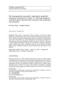
Equation (11) de nes a convex set in (p12 p22) space. These sets are depicted graphically
for each of the systems A1 A2 , and A3 in Figure 1.
1
0.8
A
2
0.6
P22
0.4
A
1
0.2
0
A
3
−0.2
−1
−0.8
−0.6
−0.4
−0.2
0
0.2
P12
Figure 1: PAi for
A1 , A2
and
A3 .
Clearly, no CQLF exists as the sets PAi i 2 1 2 3], have no common intersection (Shorten
& Narendra 2000). However, the matrix pairs fA1 A2g, fA2 A3g, fA1 A3g are pairwise
triangularizable with
2
3
2
1 0:1 7
T12 = 64
5 T23 = 64
1 1
3
2
3
17
0:1 1 7
5 T13 = 64
5:
1
;10 1
7
1 1
Hence, in general, for stable LTI systems, pairwise triangulizability of the system matrices
does not imply the existence of a CQLF.
In cases when a CQLF does not exist, the stability properties of the system must be determined using non-CQLF techniques. In the remainder of this paper, we present a novel
method for showing the global attractivity of the origin for a class of systems in the form
of Equation (1). We consider systems where the Ai matrices in A are diagonalisable, and
where any two of the Ai matrices have at least n ; 1 real linearly independent eigenvectors
in common. For certain systems of this form, the origin of the switching system is globally
attractive as veri ed in the following theorem.
Theorem 3.1.
Consider the switching system (1) with the set A de ned as follows.
Let V = fv1 : : : vn+1g be a set of real vectors, where each vi 2 IRn. Suppose any
n vectors in V are linearly independent. For each i 2 f1 2 : : : n + 1g, construct
an n n matrix Mi as follows: M1 = v1 v2 : : : vi;1 vi : : : vn;1 vn ] and for 2
i n + 1 we de ne Mi = v1 v2 : : : vn+1 vi : : : vn;1 vn], i.e. Mi is obtained by
replacing the (i ; 1)th column in M1 with the vector vn+1 . Suppose we also have p
di erent diagonal matrices D1 D2 : : : Dp with all diagonal entries negative. De ne
Ai h = MiDh Mi;1 , for 1 i n + 1 and 1 h p. Let A be a subset of
fAi h : 1 i n + 1 1 h pg.
Then the origin of the system (1) is globally attractive.
Comment : The set A de ned in Theorem 3.1 satis es the following properties:
(a) Every matrix in A is Hurwitz and diagonalisable
(b) The eigenvectors of any matrix in A are real
(c) Every pair of matrices in A share at least n ; 1 linearly independent common eigenvectors.
8
(d) Every matrix pair in A can be simultaneously triangularised (Shorten 1996).
For ease of exposition we rst present an outline of the main ideas. The proof is then developed by means of several key lemmas. Note that in the sequel we use row and column
notation interchangeably to denote vectors.
Outline of Proof
Step 1: We replace each n n matrix Mj by an (n + 1) (n + 1) matrix Mj . We
then replace each n n matrix Ai h in A by an (n + 1) (n + 1) matrix Ai h.
The matrices Ai h 2 A =4 fAi h : Ai h 2 Ag are chosen such that there is
at least one common eigenvector = (1 0 0 : : : 0) for all the matrices in A,
and also such that the properties of the solutions of the dynamic system
x_ = A(t)x A(t) 2 A
(13)
will ultimately imply the global attractivity of the origin of the system
x_ = A(t)x A(t) 2 A
where x = (x1 ::: xn) and x = (xn+1 x1 ::: xn).
9
(14)
Step 2: For a given j 2 f1 2 : : : n + 1g we consider the n + 1 linearly independent
columns of Mj . These form an n + 1 dimensional coordinate system which
includes as one of the axes. We consider the projection of the state x(t)
onto as the dynamics of the system (13) evolve. This projection is given by
the rst component of the vector
gj (t) = Mj;1x(t)
(15)
and is denoted by gj ]1(t).
Step 3: We then show that limt!1 j gj ]1(t) ; gi]1(t)j = 0 8 i j 2 f1 ::: n +1g. From
this fact we can deduce that limt!1(x1 : : : xn) = 0. This is su cient to
demonstrate the global attractivity of the origin of the system,
x_ = A(t)x A(t) 2 A:
(16)
Technical details of Proof
Lemma 3.1.
There exists a positive number a such that the set W = f(a v1) (1 v2) (1 v3) : : : (1 vn+1)g
is linearly independent in IRn+1. Here (a v1) is the vector with n + 1 coordinates, whose rst
coordinate is a and remaining n coordinates are the n coordinates of v1.
Proof :
Let V = fv1 v2 : : : vn+1g in IRn. We know that any subset of V which contains n elements
is linearly independent and thus forms a basis for IRn . Consequently, fv2 v3 : : : vn+1g forms
a basis for IRn and so there exist unique real numbers j such that v1 =
P +1 .
to be a positive number which is di erent from nj=2
j
Pn+1 v . Pick a
j =2 j j
We now show that the set W is linearly independent in IRn+1. Let v1 = (a v1) and vj =
P +1 v = 0 with at least one of the 0s non{zero. We
(1 vj ), for 2 j n + 1. Suppose ni=1
i i
i
10
P
P
+1
n+1
want to derive a contradiction. Note that 1a + nj=2
j = 0 and i=1 i vi = 0. Also note
P +1 j vj = 0 and so i = 0 for 1 i n + 1
that 1 6= 0, because if 1 = 0 then we have nj=2
P +1 j vj and a = ; 1 Pn+1 j .
and this is false. Consequently, we can write v1 = ; 11 nj=2
j =2
1
P
+1
Thus by uniqueness of j , we have j = ; j1 , for 2 j n + 1 and so a = nj=2
j , which
is false. Therefore W is linearly independent in IRn+1 . Q.E.D.
De ne Mi to be the following (n + 1) (n + 1) matrix:
0
1 b
B
B
B
0
B
B
B
B0
Mi = B
B
B
0
B
B
...
B
B
@
1 1 ::: :::1
Mi
0
1
C
C
C
C
C
C
C
C
C
C
C
C
C
C
A
where b = a (from Lemma 3.1), if i 6= 2 and b = 1, if i = 2. The change in the value of b
is because v1 only appears in Mi when i 6= 2. Note that the columns of Mi, apart from the
rst column, are vectors from the set W in Lemma 3.1.
Note that
1
0
1 s1 s2 : : : sn C
B
C
B
C
B
0
C
B
C
B
C
B
;
1
Mi;1 = B
C
0
M
i
C
B
C
B
.
.
C
B
.
C
B
A
@
0
for some real numbers s1 s2 : : : sn which depend on i.
11
De ne Dh to be the following (n + 1) (n + 1) diagonal matrix:
0
0 ::: ::: :::
B
B
B
0
B
B
B
B0
Dh
Dh = B
B
B
0
B
B
...
B
B
@
0
1
0C
C
C
C
C
C
C
C
C
C
C
C
C
C
A
De ne Ai h = Mi Dh Mi;1. We then get
0
1
0 c1 c2 : : : cn C
B
C
B
B
C
0
B
C
B
C
C
Ai h = B
B
C
0
Ai h
C
B
C
B
.
.
B
C
.
B
C
@
A
0
for some real numbers c1 c2 : : : cn which depend on i and h. Note that (1 0 0 : : : 0) is a
common eigenvector for all the m matrices Ai h.
We then have that
1
1
0
0
x_ n+1 C
xn+1 C
B
B
C
B
C
B
B
C
B
x
_1 C
x
C
B
B
1 C
C
C
B
B
C
B
B
=
A
C
B
ihB
x_ 2 C
x2 C
C
B
C
B
C
C
B
B
.
.
.
.
C
C
B
B
.
.
C
C
B
B
A
A
@
@
x_ n
if and only if
(17)
xn
0 1
0 1
x_ 1 C
x1 C
B
B
B
C
B
C
B
B
C
C
x
_
x
2
2
B
C
B
C
=
A
B
C
B
... C i h B ... C
B
C
B
C
B
@ A
@ C
A
and x_ n+1 =
n
X
i=1
ci xi
x_ n
xn
We will show that limt!1(x1 x2 : : : xn) = 0, for any solution (xn+1 x1 x2 : : : xn) to the
switching system (13). By the above, this will then imply that limt!1(x1 x2 : : : xn) = 0,
12
for any solution (x1 x2 : : : xn ) to the switching system (1) and that will give us global
attractivity of the origin in the switching system (1), and we will be done.
Let x = (xn+1 x1 x2 : : : xn). We consider the evolution of the system dynamics (13) in
each of the coordinate systems
gi = Mi;1x
(18)
There are n + 1 coordinate systems corresponding to i 2 f1 2 : : : n + 1g. Let G =
f g1]1 g2]1 : : : gn+1]1g, where gi]1 denotes the rst component of the vector gi.
Let the system dynamics be initially described by
x_ = Aj hx
(19)
over some time interval t1 t2]. Note that g_j = Dh gj . Let gj ]m be the mth component of the
vector gj and let h i denote the (i i)th diagonal entry in Dh and hence the (i + 1 i + 1)th
diagonal entry in Dh . Then we have that g_j ]m = h m;1 gj ]m, for m 6= 1 and g_j ]1 = 0.
Therefore, when we are in system (19), we have
gj ]m(t) = gj ]m(t1) e h m;1(t;t1) for m 6= 1
(20)
and gj ]1 is a constant function of t.
The members of G, when we are in system (19), are illustrated in Figure 1. Note that gj ]1
is a constant function of time over t1 t2] while the other gj ]m's vary with time according to
(20).
-
gi]1
gj ]1
gm ]1
gk ]1
+
Figure 2: Members of the set G.
Consider the evolution of gi]1 relative to gj ]1. This `distance' denoted by di j (t), is given by
di j (t) = j gi]1(t) ; gj ]1(t)j
13
(21)
and can be conveniently calculated from
gi = Mi;1 Mj gj
(22)
We now analyse the structure of the matrix Fi j = Mi;1Mj , for i 6= j . We see that 1 always
appears in the rst row rst column entry of Fi j . We claim that there is only one other
non{zero entry in the rst row.
Lemma 3.2.
If we exclude the rst column of the matrix Fi j , for i 6= j , then there is only one non{zero
entry (denoted by Ci j k ) in the rst row. Ci j k appears in the kth column where k = j , when
i = 1, and k = i, when i 6= 1. Note that k is never 1.
Proof :
Denote the rst row of Mi;1 by ~r. Suppose rst that i = 1. We see that a basis for the
orthogonal complement of ~r in IRn+1 is given by f(a v1) (1 v2) (1 v3) : : : (1 vn )g. Hence,
using the result of Lemma 3.1, the only place (apart from the rst column) in the rst row of
Fi j which is non{zero, is the kth column where k is the number of the column in Mj which
has (1 vn+1). Thus k = j . Here Ci j k is the dot product of ~r and (1 vn+1).
Suppose next that i = 2. We see that a basis for the orthogonal complement of ~r in IRn+1 is
given by f(1 v2) (1 v3) : : : (1 vn+1)g. Hence, as above, the only place (apart from the rst
column) in the rst row of Fi j which is non{zero, is the kth column where k is the number
of the column in Mj which has (a v1). Thus k = 2. Here Ci j k is the dot product of ~r and
(a v1).
Suppose nally that i > 2. We see that a basis for the orthogonal complement of ~r in IRn+1 is
obtained by deleting (1 vi;1) from the set W in Lemma 3.1. Hence, as above, the only place
(apart from the rst column) in the rst row of Fi j which is non{zero, is the kth column
where k is the number of the column in Mj which has (1 vi;1). Thus k = i. Here Ci j k is
the dot product of ~r and (1 vi;1). Q.E.D.
14
We combine Lemma 3.2 with (22) to obtain
gi]1 = gj ]1 + Ci j k gj ]k for 1 i n + 1 with i 6= j:
(23)
Note that (23) is true irrespective of what system we are in.
We combine (20) and (24) to obtain
gi]1(t) ; gj ]1(t) = Ci j k gj ]k (t1) e h k;1(t;t1) for i 6= j
(24)
whenever we are in system (19). Hence
di j (t) = jCi j k jj gj ]k (t1)j e h k;1(t;t1) for t1 t t2 and i 6= j:
Consequently ddidtj (t) < 0, or else gi]1 and gj ]1 both agree over the time interval t1 t2]. Thus
the distance between gi]1(t) and the constant gj ]1(t) is either getting smaller or always zero
over the time interval t1 t2], when we are in the system described by x_ = Aj hx.
Proof of Theorem 3.1 :
We will now prove that limt!1 (x1 x2 : : : xn) = 0, for any solution (x1 x2 : : : xn) to the
system (1) with the set A de ned as in statement of Theorem 3.1, and then we will be done.
Denote the maximum value (minimum value) of G(t), for a time t in the time interval t1 t2],
by max1 G(t) (min1 G(t)). Recall that we are in system (19) when t 2 t1 t2]. Then
max1 G(t) ; min1 G(t) = gi]1(t) ; gr ]1(t) for some i r 2 f1 2 : : : n + 1g
= gi]1(t) ; gj ]1(t) + gj ]1(t) ; gr ]1(t)
= jCi j k j j gj ]k (t1)j e h k;1(t;t1) + jCr j qj j gj ]q (t1)j e
h q;1 (t;t1 )
where, as in Lemma 3.2, k = j , if i = 1, and k = i, if i 6= 1. Similarly q = j , if r = 1, and
q = r, if r 6= 1. Note that if gj ]1 is a maximum value (or minimum value) of G(t), then
the last line above collapses to just one term instead of two, and in this case the following
arguments will also work. Now let Bi j t1 = jCi j k j j gj ]k (t1)j = distance between gi]1(t1) and
gj ]1(t1). Let Br j t1 = jCr j q j j gj ]q (t1)j = distance between gj ]1(t1) and gr ]1(t1). Also let
15
= maxf
:1
ng. Note that < 0. Then
p 1
max1 G(t) ; min1 G(t)
(Bi j t1 + Br j t1 ) e (t;t1)
(max1 G(t1) ; min1 G(t1)) e
(t;t1)
(25)
The last inequality follows from the fact that, over the time interval t1 t2], gi]1(t) remains
on the same side of the constant gj ]1(t) and gr]1(t) remains on the other side of gj ]1(t).
This is because the right hand side of (24) does not change sign as time changes over the
time interval t1 t2]. Note that i and r may change with time and so max1 G(t1) may not
correspond to gi]1(t1), and min1 G(t1) may not correspond to gr ]1(t1).
Now suppose we switch to the next (second) system described by
x_ = Ac w x
(26)
over the time interval t2 t3]. Denote the maximum value (minimum value) of G(t), for some
time t 2 t2 t3], by max2 G(t) (min2 G(t)). Then as above we get
max2 G(t) ; min2 G(t)
(max2 G(t2) ; min2 G(t2)) e
(t;t2)
(max1 G(t1) ; min1 G(t1)) e
(t2;t1 )
(max1 G(t1) ; min1 G(t1)) e
(t;t1)
e (t;t2)
The second inequality above follows from the fact that we start the second system (26) at
time t2 when we stop the rst system (19), and the initial conditions for the second system
are the terminal conditions for the rst system at time t2. Thus max2 G(t2) ; min2 G(t2)
(max1 G(t1) ; min1 G(t1)) e (t2;t1) from (25).
Now suppose we switch to the next (third) system described by
x_ = Ad ux
(27)
over the time interval t3 t4]. Denote the maximum value (minimum value) of G(t), for some
time t 2 t3 t4], by max3 G(t) (min3 G(t)). Then as above we get
max3 G(t) ; min3 G(t) (max1 G(t1) ; min1 G(t1)) e
16
(t;t1)
For the general suituation, when we have switched for the mth time, we are in the system
described by x_ = Az lx over the time interval tm tm+1]. Again we denote the maximum
value (minimum value) of G(t), for some time t 2 tm tm+1], by maxm G(t) (minm G(t)).
Then as above we get
maxm G(t) ; minm G(t) (max1 G(t1) ; min1 G(t1)) e
(t;t1)
Therefore, since < 0, we have limt!1 (max G(t);min G(t)) = 0, where max G(t) (min G(t))
denotes the maximum value (minimum value) of G(t) for any time t t1. Thus
lim j gi]1(t) ; gj ]1(t)j = 0 for all i j 2 f1 2 : : : n + 1g:
t!1
lim jCi j k jj gj ]k (t)j = 0 where k = j if i = 1 and k = i if i 6= 1 and i 6= j:
t!1
lim j gj ]k (t)j = 0 for j 2 f1 2 : : : n + 1g and k 2 f2 3 : : : n + 1g:
t!1
The second line above follows from (23), which is independent of what system we are in.
The last line above follows from the fact that the Ci0sj k form a nite collection of non{zero
numbers when i 6= j . Also note that the last line above might not hold for k = 1 because
then i = j = 1. Therefore, since limt!1 x(t) = limt!1 Mj gj (t), we get
0
1
xn+1 C
B
B
C
B
C
x
B
1 C
B
C
B
C
lim B
C
t!1 B x2 C
B
... C
B
C
B
C
@
A
=
xn
0 1
x1 C
B
C
B
C
B
x
2
B
lim B C
C
t!1 B .. C
. C
B
@ A
xn
0
1 b
B
B
B
0
B
B
B
B
0
B
lim
t!1 B
B
0
B
B
...
B
B
@
1 1 :::
Mj
0
=
0
BB 0
BB 0 Mj
lim B
t!1 B ..
B@ .
0
17
10
B
C
B
C
B
C
B
C
B
C
B
C
C
@
AB
1
:::1 C
1
0
C
C
gj ]1(t) C
C
B
C
C
B
C
C
B
g
]
(
t
)
C
j
2
C
B
C
C
B
C
.
B
C
..
C
B
C
C
@
A
C
C
C
A gj ]n+1(t)
1
gj ]1(t) C
C
gj ]2(t) C
C
C
...
C
C
A
gj ]n+1(t)
=
0 1
0C
B
B
C
B
0C
B
C
B
C
.
B
C
.
.
B
@ C
A
0
Thus
lim (x1 x2 : : : xn) = 0
t!1
and we have global attractivity of the origin in the switching system (1). Q.E.D.
4 Concluding remarks
In this paper we have shown global attractivity for a class of switching systems. This result
is important for a number of reasons. Primarily, it can be readily shown from Example 1,
or by using examples generated from standard convex optimization packages, such as the
MATLAB LMI toolbox (Gahinet, Nemirovski, Laub & Chilali 1995), that the condition of
pairwise triangularisability is not su cient to guarantee the existence of a CQLF. Hence,
in cases where no CQLF exists, qualitative statements concerning system stability, must be
validated using other techniques. One such technique is presented in this paper namely, a
technique which proves global attractivity by embedding the original (n-dimensional) state
space in a higher (n + 1) dimensional state space. This technique can be used to prove
the global attractivity in cases when a CQLF does not exist, and it is likely that derived
methodology is applicable to a wide class of related switching systems.
The derived results also suggest that the condition of simultaneous triangularisability may
be relaxed signi cantly without the loss of asymptotic stability1. This observation will form
the basis of future work. It is hoped that more results will be reported at a later date.
Note that the concepts of stability and attractivity are not equivalent see Narendra & Annaswamy
(1989).
1
18
Acknowledgements
This work was partially supported by the European Union funded research training network
Multi-Agent Control, HPRN-CT-1999-00107. The rst author gratefully acknowledges many
discussions with Professor K.S. Narendra.
19
References
Barker, G. P., Berman, A. & Plemmons, R. J. (1978), `Positive Diagonal Solutions to the
Lyapunov Equations', Linear and Multilinear Algebra 5(3), 249{256.
Cohen, N. & Lewkowicz, I. (1997), `Convex Invertible Cones and The Lyapunov Equation',
Linear Algebra and its Applications 250(1), 105{131.
Gahinet, P., Nemirovski, A., Laub, A. & Chilali, M. (1995), LMI Control Toolbox for use
with MATLAB, The Mathworks Inc.
Liberzon, D., Hespanha, J. P. & Morse, S. (1998), Stability of Switched Linear Systems: A Lie
Algebraic Condition, Technical report, Laboratory for Control Science and Engineering,
Yale University.
Mori, Y., Mori, T. & Kuroe, Y. (1996), Classes of Systems having Common Quadratic Lyapunov Functions: Triangular System Matrices, in `proceedings of Electronic Information
and Systems Conference (in Japanese)'.
Mori, Y., Mori, T. & Kuroe, Y. (1997), A Solution to the Common Lyapunov Function
Problem for Continuous Time Systems, in `proceedings of 36th Conference on Decision
and Control'.
Narendra, K. & Annaswamy, A. (1989), Stable Adaptive Systems, Prentice-Hall.
Narendra, K. & Taylor, J. (1973), Frequency Domain Criteria for Absolute Stability, Academic Press.
Narendra, K. S. & Balakrishnan, J. (1994), `A Common Lyapunov Function for Stable
LTI Systems with Commuting A-Matrices', IEEE Transactions on Automatic Control
39(12), 2469{2471.
Shorten, R. (1996), A Study of Hybrid Dynamical Systems with Application to Automotive
Control, PhD thesis, Department of Electrical and Electronic Engineering, University
College Dublin, Republic of Ireland.
20
Shorten, R. & Narendra, K. (1998a), Neccessary and Su cient Conditions for the Existence
of a Common Lyapunov Function for Two Second Order Systems, Technical report,
Center for Systems Science.
Shorten, R. & Narendra, K. (1998b), On the Stability and Existence of Common Lyapunov
Functions for Linear Stable Switching Systems, In proceedings of Conference on Decision
and Control, Florida Dec 15th-18th.
Shorten, R. & Narendra, K. (2000), Necessary and Su cient Conditions for the Existence of
a Common Lyapunov Function for M Second Order Systems, Technical report, Center
for Systems Science (in preparation).
Shorten, R. N., O Cairbre, F. & Curran, P. F. (2000), On the dynamic instability of a class
of hybrid systems, in `Proceedings of IFAC conference on Arti cial Intelligence in Real
Time Control'.
Vidysagar, M. (1993), Nonlinear Systems Analysis, Prentice Hall.
21