Download Report

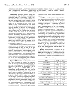
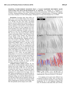
46th Lunar and Planetary Science Conference (2015)
2848.pdf
FREQUENCY DISTRIBUTIONS OF TOPOGRAPHIC SLOPES ON THE MOON. M. A. Kreslavsky1,2,
A. Yu. Bystrov2, I. P. Karachevtseva 1Earth and Planetary Sciences, University of California - Santa Cruz, Santa
Cruz, CA, USA, [email protected], 2MExLab, Moscow State University of Geodesy and Cartography (MIIGAiK),
Moscow, Russia.
Introduction: Statistical characterization of topographic slopes is a valuable tool for comparison of
planetary landscapes and understanding of landscape
evolution processes. It also gives essential engineering
information need for exploration activity. Here we follow up earlier LOLA-based studies [1] with addition of
short-baseline slope data from the digital terrain models (DTM) derived from LROC NAC stereo images
[2]. We also briefly list relevant theoretical background, which has not been properly presented in the
planetary science literature.
Theoretical background: The usual quantity of interest, "slope" s, also dubbed as "2D slope" is defined
as the absolute value of gradient vector of surface elevation calculated at certain baseline. On the other hand,
it is often much easier and more accurate to measure
not the gradients, but slopes p along linear profiles
across the surface, also dubbed "1D slopes". The relationship between statistical properties of 1D and 2D
slopes [e.g., 3] can be established in the frame of a
theoretical stochastic model that considers the topographic gradient as an isotropic random vector. The isotropy assumption is often reasonable for the Moon and
other bodies with landscapes dominated by impacts,
but it fails for many terrestrial, martian, etc. landscapes. Under the isotropic assumption, the probability
density functions f1D(p) and f2D(s) of 1D and 2D slopes
are related to each other through the following modification of the Abel transform:
1 ∞ f 2 D ( s )ds
;
(1)
f 1D ( p) =
π | p| s 2 − p 2
∫
f 2 D ( s ) = −2
d
ds
∫
∞
s
f1D ( p) pdp
p2 − s2
.
(2)
This transform can be numerically applied to empirical
frequency distributions as proxies for the probability
densities. The (cumulative) distribution function
F2D(s), the probability that the absolute value of the
gradient is above s,
∞
∞ f ( p ) pdp
1D
.
(3)
F2 D ( s ) = f 2 D ( s ' )ds ' = 2
s
s
p2 − s2
∫
∫
is a proxy for the proportion of area tiled steeper than
s. The singularity under integrals in (1) - (3) requires
special numerical integration algorithms.
Note that "slopes" p and s above are the tangents of
slope angles. The probability density function fa(θ) of
slope angle θ in degrees is related to the probability
density f of tanθ as the following:
f a (θ) = π 180 f (tan θ) cos 2 θ ;
(
2
(4)
)
f (t ) = 180 π f a (arctan t ) 1 + t .
(5)
Data processing. For this study we selected several LROC NAC DTM products [2] to study shortbaseline slopes and larger test areas surrounding each
DTM to study longer-baselines slopes with LOLA
data. We selected only those DTM that represented
typical geologically homogeneous terrain away from
large young craters, prominent linear topographic features, etc. We also excluded DTM with gaps due to
shadows in the original stereo images. For each selected DTM we also chose a circular geologically homogeneous area containing the DTM (not necessarily
in its center). We chose the circle diameter of 150 km,
except Apollo-14 landing site, where we used diameter
of 90 km to place the whole test area within the contiguous patch of Fra Mauro Formation.
Slopes from LOLA data. We used individual LOLA
profiles from the circular LRO orbit. We calculated 1D
slopes between consecutive laser shots, which gave the
baseline of 57.5 m, as well as slopes at 4×, 16×, and
64× longer baselines (230 m, 920 m, and 3.7 km).
Typically we obtained ~6×105 slopes for each sample
site and each baseline. Each LOLA laser shot was split
into 5 spots giving 5 elevation measurements [4]. We
also calculate slopes between spots 1-2, 1-3, 1-4, and
1-5 and thus obtained 1D slopes at 25 m baseline, ~106
slopes for each sample site. We generated slope histograms with 0.1º increment in slopes and thus obtained
slope-frequency distributions; examples are shown in
Fig. 1. Using (3) we calculated distributions of 2D
slopes and derived the median slopes (Fig. 2).
Slopes from LROC NAC DTM. The DTM pixels are
2 m in size. Statistics of slopes the shortest possible, 2
m baseline is significantly distorted by peculiarities of
the interpolation algorithm used in the process of DTM
generation. To mitigate this problem we smoothed the
DTM using ArcGIS tools, namely "5x5 blur" repeated
4 times. Our analysis showed that this smoothing procedure is equivalent to Gaussian low-pass filter with
the half-width of σ = 2.13 pixels. Then we calculated
2D slopes at each pixel. The effective baseline of these
slopes is defined by the smoothing procedure; we consider 2σ (8.5 m) as a proxy to it. We generated slope
histograms with 0.5º increment in slopes and thus obtained incremental slope-frequency distributions.
For many sample sites, the median 2D slopes at 8.5
m baseline turned out to be somewhat lower than ex-
46th Lunar and Planetary Science Conference (2015)
is proportional to exp(-p/tanθh), where parameter
θh = 6.0º is the same for all highland samples. Thus,
km-scale topography of the highlands have a universal
slope parameter of ~6º; its physical nature is unclear.
10
Luna 20
5
Median slope, deg
pected from extrapolation of longer-baseline LOLA
data (see "Luna 16" site in Fig. 2). This is probably
caused by the difference in the slope measurement
technique. Individual LOLA laser spots (~5 m size) are
much smaller than the baseline, which causes leakage
of high-spatial-frequency topographic signal, while for
the smoothed DTM the effective spot size is equal to
the effective baseline, and no such leakage occurs.
We used (1) to recalculate 2D slope distributions
into 1D slope distributions, and compared them with
25 m baseline results from LOLA (Fig. 1). We saw
good agreement in the distribution shapes.
2848.pdf
3
Apollo 14
2
1
Luna 16
Baseline: 25 m
Frequency
0.5
10
Luna 20
100
1000
Baseline, m
Luna 16
0
10
Fig. 2. Scale dependence of the median slope for typical
highlands (Luna 20), typical maria (Luna 16), and Fra Mauro
Formation (A14).
A14
20
1D slope, deg
30
Fig. 1. Incremental frequency distribution of 1D slopes at 25
m baseline for typical highlands (Luna 20), typical maria
(Luna 16), and Fra Mauro Formation (A14). Note log scale
on the vertical frequency axis.
Results: The slope-frequency distributions on the
Moon have a rich structure (Fig. 1). All distributions
have significant steep-slope tails. They show distinctive rollover starting at ~25º 1D slopes; there are virtually no slopes steeper than ~36º. This rollover is apparently related to the angle of repose. There are no processes on the Moon that could effectively produce short
slopes steeper than the angle of repose (on the Earth
water erosion is doing that).
Highlands. For each of our typical highland samples, the slope distributions are almost the same for
different baselines, excluding the longest one; consequently, the median slopes do not change with scale.
This is consistent with the Hurst exponent of ~1 reported for highlands in [1]. This means that all shortbaseline slopes are actually inherited from larger,
kilometer-scale topographic forms. Contribution of
smaller objects into slope distribution is negligible.
Different highland samples have somewhat different median slopes, however, the distributions show that
the difference is due to different proportions of area
with slopes below ~5º, while in a wide slope range
from ~5º to ~25º the distribution in linear in the loglinear plot (Luna 20 in Fig. 1), which means that f1D(p)
Maria. Our typical mare samples have remarkably
similar slope distributions. They have sharp wellpronounced low-slope peak whose width defines the
median slope, heavy peak shoulder that grades into the
steep-slope tail. The latter is obviously related to walls
of fresh craters. For longer baselines the peak with its
shoulder becomes narrower, preserving its general
shape and just suggesting some fractal-like topography.
Apparently it is formed by equilibrium between emplacement of small craters and their obliteration by
regolith gardening [5].
Other samples. At the sorter baselines, the Fra
Mauro Formation (A14 in Fig. 1) is similar to highlands, but much smoother with θh = 3.7º, while at the
longer baselines the distribution grades into mare-like.
The vicinity of Bhabha crater in the South Pole Aitken basin in LOLA data clearly shows ~1:1 mixture
of typical mare and typical highland slope distributions
at all baselines, which perfectly corresponds to the geological nature of the terrain. LROC DTM does not
sample maria, and the derived distribution is indeed
similar to highlands, but with rather low median slope.
Conclusions: Slope-frequency distributions are a
rich data set worth of further more systematic analysis.
References: [1] Rosenburg M. et al (2011) JGR, 116,
E02001. [2] Robinson M. et al. (2010) Space Sci. Rev., 102,
293. [3] Aharonson O. and Schorghofer N. (2006) JGR, 111,
E11007. [4] Smith D. et al. (2010) GRL, 37, L18204.
[5] Kreslavsky M. et al.. (2013) Icarus, 226, 52.
Acknowledgements: This work was carried out at
MIIGAiK and supported by Russian Science Foundation,
project 14-22-00197.