
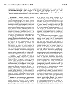
How does the double layer at a disk electrode
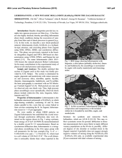
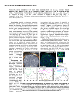
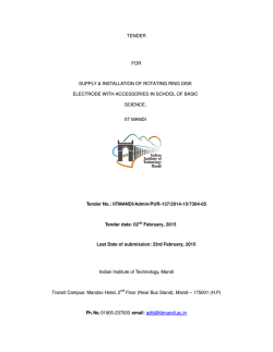
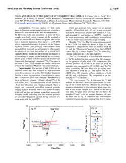
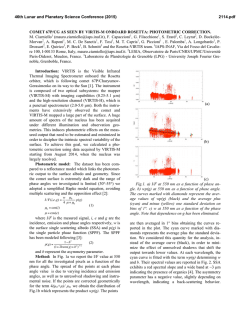
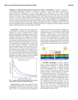
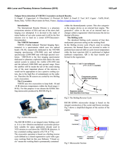
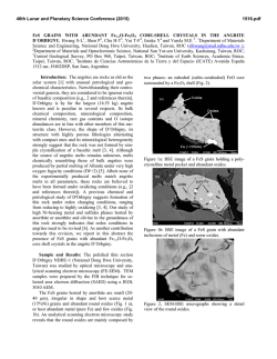
Journal of
Electroanalytical
Chemistry
Journal of Electroanalytical Chemistry 575 (2005) 81–93
www.elsevier.com/locate/jelechem
How does the double layer at a disk electrode charge?
Jan C. Myland, Keith B. Oldham
*
Department of Chemistry, Electrochemical Laboratory, Trent University, Peterborough, Ont., Canada K9J 7B8
Received 1 June 2004; received in revised form 1 September 2004; accepted 2 September 2004
Available online 28 October 2004
Abstract
Because of the nonuniform accessibility of its surface to ion transport from the solution, the double layer at an inlaid disk electrode charges anomalously in response to a potential step. A numerical simulation of the problem shows that the overall current
versus time transient differs little from that for a single resistor in series with a single capacitor. Nevertheless, the charging process,
away from the diskÕs perimeter, differs surprisingly from what might be expected in that the current density initially increases with
time.
Ó 2004 Elsevier B.V. All rights reserved.
Keywords: Double layer; Disk electrode; Chronoamperometry; Charging current; Simulation; Spheroidal coordinates; Potential step
1. Introduction
Though historically it has provided us with a credible
picture of the electrodejsolution interface, the charging
of the double layer is nowadays regarded as a nuisance
by most electrochemists. There are several interrelated
difficulties caused by the charging current. It adds to,
and thereby interferes with the measurement of, the
chemically more interesting faradaic current. It corrupts
applied signals. And its sluggishness limits the rapid faradaic response necessary for the study of fast electrochemical or chemical reactions [1]. Knowledge of how
the double-layer charges is necessary if its effects are to
be recognized and obviated.
In an electrolyte solution of infinite conductivity, the
double layer would charge instantaneously in response
to a potential perturbation. The attempt to approach
this ideal is one of the reasons for adding excess supporting ions in electrochemical experiments, but the conductivity j, typically 1 S m1, cannot conveniently be
increased beyond about 10 S m1, even when the solvent
*
Corresponding author. Tel.: +1 705 748 1011x1336; fax: +1 705
748 1625.
E-mail address: [email protected] (K.B. Oldham).
0022-0728/$ - see front matter Ó 2004 Elsevier B.V. All rights reserved.
doi:10.1016/j.jelechem.2004.09.004
is water. Electronic negative feedback [2,3] can be an
alternative to increasing the conductivity, but is itself a
source of complication.
The model generally adopted for double-layer charging is purely electrical: a resistor of constant resistance R
in series with a capacitor of constant capacitance C. In
response to a potential step of magnitude DE, the exponentially decaying current
IðtÞ ¼
DE
t
exp
;
R
RC
ð1:1Þ
flows according to this model. The capacitance is taken
to be proportional to the area A of the solution/electrode junction through a constant c (typical magnitude
0.1 F m2), the capacitivity or specific capacitance of
the interface. This model is reasonable for a large planar
electrode separated by a constant distance L from a second electrode, also of area A, in which case the resistance is calculable from the formula
L
:
ð1:2Þ
R¼
jA
Seldom, however, do the cells used in electrochemical
experiments have geometries to which this latter formula
may be justifiably applied, though it nevertheless sometimes is.
82
J.C. Myland, K.B. Oldham / Journal of Electroanalytical Chemistry 575 (2005) 81–93
Eq. (1.1) also applies when a sessile hemispherical
electrode is subjected to a potential step, with the auxiliary electrode being large and remote. Because it is relevant to the prime purpose of this paper, it is instructive
to derive Eq. (1.1) for the hemispherical electrode and
this will be accomplished in Section 3. Preceding this,
in Section 2, we discuss some fundamental aspects of
the electrode/solution system.
Hemispherical electrodes are a favourite tool of theorists, but in practice it is the disk electrode that is in general use experimentally, and that is the main subject of
this study. Faradaic processes at inlaid disk electrodes
are often treated theoretically as if they were hemispheres [4] and, by default, non-faradaic processes at
disks have been considered to obey Eq. (1.1). It has been
pointed out recently [4], however, that the simple model
of a single resistor in series with a single capacitor does
not apply to the disk electrode, irrespective of its size.
The reason can best be appreciated by considering the
disk to be subdivided into a number N of annuli, all
of the same area and hence of equal capacitance. The
resistances that each of these annuli ‘‘sees’’ in the surrounding solution are different, because of the easier
accessibility of the annuli near the perimeter to ionic
transport from the solution. Note that had we similarly
dissected a hemispherical electrode, the N resistances
would have been identical. It is not difficult to calculate
the magnitudes of the N resistors for the disk and hence
to find the net effect. This has been carried out (for
N = 1) and the result [4] is to replace Eq. (1.1) by
t t i
DE h
t
IðtÞ ¼
exp
Ei
þ
;
ð1:3Þ
R
2RC
2RC
2RC
where Ei( ) denotes the exponential integral function.
However, Eq. (1.3) is not the whole story and it can
be expected to apply only for short times. Returning
to the N-unit model, one must recognize that, because
the current in each unit is different, the N capacitors
charge at different rates. In consequence, the outer surface of the double layer, the ‘‘Helmholtz plane’’ in the
Gouy–Chapman model, ceases to be an equipotential
surface. In turn, this alters the route followed by the current through the electrolyte solution. In effect, the resistors with which the N capacitors are in series come to
have time-dependent magnitudes, a feature that Eq.
(1.3) does not recognize but which will be incorporated
in the present study.
2. Some fundamentals
Under consideration here is the junction between a
metal (or some other excellent conductor) and an electrolyte solution. No chemical or electrochemical reaction can occur at this interface, and no specific
adsorption of ions takes place. Though the conclusions
Fig. 1. A double layer is formed at the junction of an inlaid disk
working electrode and adjacent electrolyte solution. Point S lies on the
Helmholtz plane of that electrode, whereas point B is similarly
positioned on the large auxiliary electrode. A hemispherical electrode,
shown inset, replaces the disk for the discussion in Section 3.
of this study are largely independent of the wider environment of the interface, for concreteness we take the
interface to be the ‘‘working electrode’’ of a cell in which
the second, auxiliary, electrode is a hemispherical dome
of the same metal as the working electrode and of such a
large radius that is effectively ‘‘at infinity’’. Our objective
is to study a working electrode in the shape of the disk
shown in cross section in Fig. 1, but also of concern is
the case in which a sessile hemispherical electrode replaces the disk, as in the inset to Fig. 1. The remaining
boundary of the cell is an insulating horizontal plane.
An electrical double layer normally exists at such an
electrode but we assume (only for convenience) that
no such layer is present initially, so that the electrical
potential is uniform throughout the solution, having a
value that we take to be / = 0, and there is no charge
density anywhere. At time t = 0, the switch shown in
Fig. 1 is thrown, current commences to flow, and a double layer is established. Our prime interest is in the time
dependence, I(t), of the current. The sign attaching to I
is such that electricity flowing through the working electrode from the metal into the electrolyte solution is positive, thereby conforming to the electrochemical
convention of anodic current being positive though, of
course, the term ‘‘anode’’ is inapplicable here in the absence of a faradaic process. Electric charge is conveyed
conductively through the electrolyte solution. Although
the polarized electrode does not allow the passage of
current through itself, an apparent flow of electricity is
possible transiently, because positive charges (electron
holes) accumulate on the surface of the metal, while a
negative ionic charge builds up in solution at the interface. To a good approximation, the double layer in these
circumstances behaves as a capacitor.
The properties of points S, in solution at the Helmholtz plane adjacent to the working electrode, are of
interest. The locus of such points serves as the second
J.C. Myland, K.B. Oldham / Journal of Electroanalytical Chemistry 575 (2005) 81–93
‘‘plate’’ of the double-layer ‘‘capacitor’’, and the potential there appears in the equation
i ¼ c
o
ð/ EÞ
ot s
ð2:1Þ
that describes the capacitive behaviour. In practice the
capacitivity frequently varies somewhat with potential,
but here we ignore this aspect and treat c as a constant.
In the equation above i is the current density (A m2)
passing ‘‘through’’ the interface. The potential of point
S (with respect to a point B on the Helmholtz plane of
the auxiliary electrode) is represented by /s, whereas E
is the metallic potential of the working electrode (with
respect to that of the auxiliary electrode) which
changes from 0 to DE at time t = 0. The Gouy–Chapman theory [5] describes the electrical properties of the
double layer just beyond point S, but our interest here
is in much larger distances from the electrode where
the influence of current flow outweighs that of the
non-electroneutrality due to the proximity of the double layer.
Electricity passing through points S spreads throughout the electrolyte solution and exits capacitively
through the auxiliary electrode, which is large enough
to be unperturbed thereby. Its passage through the ionic
medium is governed by two laws: LaplaceÕs law describes the spatial distribution of potential
r2 / ¼ 0
ð2:2Þ
and OhmÕs law in the form
o/
ik ¼ j
o‘
ð2:3Þ
relates the local current density i to the gradient of
potential. In these equation $2 is the laplacian operator,
examples of which will be found in Eqs. (3.1) and (4.10)
in later sections, and ‘ is some metric coordinate. The i
subscript is a reminder that the equation gives the component of the current density in the direction parallel to
the ‘ coordinate.
If we always choose a coordinate ‘ that passes
through S and is normal to the interface at that point,
then we can equate the current densities that appear in
Eqs. (2.1) and (2.3). And if, moreover, the potential E
of the metal is constant, then the two equations combine
into the appealingly simple result
o/
o/
c
¼j
:
ð2:4Þ
ot s
o‘ s
The problems addressed in this study are essentially
those of solving Eq. (2.2) when (2.4) is one of the boundary conditions. This problem is solved for the case of a
hemispherical interface in Section 3, and for the much
more difficult case of a disk-shaped interface in the
remainder of the article.
83
3. The hemispherical double layer
One objective of this section is to derive Eq. (1.1) by
solving the equations from Section 2 for the case of a
hemispherical electrode of radius rs, and thereby to
throw light on the features of the charging process.
In spherical coordinates, with angular symmetry, the
laplacian operator adopts a simple form, Eq. (2.2)
becoming
0 ¼ r2 / ¼
o2 / 2 o/
þ
or2 r or
for rs 6 r < 1:
ð3:1Þ
With / a function /(r, t) of both the radial coordinate r
and time t, we seek a solution to this differential equation subject to the initial conditions
/ðr; 0Þ ¼ 0;
rs < r < 1
ð3:2Þ
and
/ðrs ; tÞ ¼ E ¼
0;
t < 0;
DE; t > 0:
ð3:3Þ
The second of these recognizes that, because a capacitor
offers no immediate impedance to a potential step, the
sudden change in the metal potential from 0 to DE is
echoed immediately by the potential of points S on the
outer face of the double layer. The two boundary conditions are
/!0
as r ! 1
ð3:4Þ
and
o/
o/
c
¼j
:
ot s
or s
ð3:5Þ
The latter is simply Eq. (2.4) with ‘ replaced by r in
recognition that the radial coordinate is metric and normal to the hemispherical interface.
One integration of LaplaceÕs equation (3.1) gives
o/ ðan r-independent termÞ f ðtÞ
¼
¼ 2
or
r2
r
and a second integration then yields
/ ¼ ðconstantÞ f ðtÞ f ðtÞ
¼
r
r
ð3:6Þ
ð3:7Þ
the equating of the ‘‘constant’’ to zero being a consequence of condition (3.4). Here f(t) is some presently unknown function of time. It can be determined by
specializing Eqs. (3.6) and (3.7) to r = rs and then invoking condition (3.5). This gives the differential equation
jf ðtÞ c df
¼
r2s
rs dt
ð3:8Þ
that solves to
jt
f ðtÞ ¼ ðconstantÞ exp
crs
ð3:9Þ
84
J.C. Myland, K.B. Oldham / Journal of Electroanalytical Chemistry 575 (2005) 81–93
Accordingly, after the latest ‘‘constant’’ is identified
as rsDE by recourse to condition (3.3), one finds
rs DE
jt
exp
ð3:10Þ
/ðr; tÞ ¼
r
crs
as the final comprehensive solution.
The current density at the interface, and hence the total current can be found from Eq. (2.1):
d
IðtÞ ¼ 2pr2s is ¼ 2pcr2s /ðrs ; tÞ
dt
jt
¼ 2pjrs DE exp
:
crs
ð3:11Þ
Our task is now complete, this result being equivalent to
Eq. (1.1) because R = 1/(2pjrs) and C ¼ 2pcr2s . Notice
that, unlike the problems with which electrochemists
are most familiar, time entered this partial–differential
equation problem only via a boundary condition.
A division of the previous two equations reveals the
equation
/ðr; tÞ
1
¼
IðtÞ
2pjr
ð3:12Þ
reminiscent of OhmÕs law in its familiar form (voltage)/
(current) = (resistance). It shows that the resistance between any hemisphere of fixed radius r, where the
potential is /(r,t), and a hemisphere of infinite radius,
where the potential is zero, is the time-independent
constant 1/(2pjr). We shall make use of this result in
Section 6.
Eq. (3.10) implies that at t = 0 the potential at any
point on a hemisphere of radius r immediately changes
from zero to
/ðr; 0Þ ¼
rs
DE:
r
ð3:13Þ
Likewise the current density at that site is predicted to
jump discontinuously to the value jrsDE/r2. Electric
fields and charges can travel very fast, but not at infinite
speed. A partial explanation of this anomaly is that
PoissonÕs law,
r2 / ¼
q
e
ð3:14Þ
more closely describes the behaviour of electrified
phases than does the Laplace equation. Here e denotes
the permittivity (F m1) of the medium and q represents
the local charge density (C m3). It can be shown that,
in a resistive medium, q decays in obedience to an
exp(jt/e) law. In electrochemical systems the permittivity-to-conductivity ratio is of nanosecond magnitude,
so the approximation implied by the use of LaplaceÕs
equation is small enough to evade experimental detection, except very close to interfaces.
Thus, there are two time constants governing the
charging of the hemispherical double layer: the e/j time
constant, and the crs/j time constant evident in Eqs.
(3.10) and (3.11). The latter is rarely less than 1 ls in
electrochemical practice. Except when electrodes are so
small that their dimensions are comparable to the double-layer thickness, these two time constants are so well
separated that the responses to them may be treated as
two separate consecutive stages in the charging of the
double layer by a potential step. The first of these, Stage
One, occurs almost instantaneously and results in the
potential distribution described in Eq. (3.13) becoming
established. Stage Two follows, the distribution that it
engenders being described by Eq. (3.10). Both equations
are inexact inasmuch as each denies the existence of the
other. Moreover, neither equation recognizes the existence or motion of free charge. Nonetheless, we believe
that both equations are excellent approximations to
the truth.
4. Oblate spheroidal coordinates
The spherical coordinate system that we employed
in the previous section was clearly the best system for
that purpose, far better than cartesian or cylindrical
coordinates, for example. In a similar way, oblate spheroidal coordinates constitute the ‘‘natural’’ system for
the geometry of the cell shown in Fig. 1. This coordinate system has been employed or discussed previously
[6–16] in electrochemical studies involving disk
electrodes.
Though there is another representation [17] that
avoids the use of trigonometric and hyperbolic functions, the most usual definition of the three oblate spheroidal coordinates is through the following relationships
[18] to cartesian coordinates
x ¼ a cosh n cos g cos h;
ð4:1Þ
y ¼ a cosh n cos g sin h;
ð4:2Þ
z ¼ a sinh n sin g:
ð4:3Þ
In the present context, a is the radius of the disk electrode. Unlike the other two coordinates which are angular, n takes values in the range 0 6 n < 1, being equal to
zero on the diskÕs surface. In the present application, g
adopts values in the 0 6 g 6 p/2 range, being zero on
the surface of the insulating surface and equal to p/2
on the cellÕs axis of rotational symmetry. The third coordinate h corresponds to a longitudinal angle, taking values between 0 and 2p, but is of minor importance in the
present cell on account of the rotational symmetry.
Fig. 2 shows, in cross section, the shapes of surfaces of
constant n, which are generally ellipses in cross section,
and those of constant g, which are mostly hyperbolas.
If a point in space has the oblate spheroidal coordinates n, g, h and a second point, very close to the first,
J.C. Myland, K.B. Oldham / Journal of Electroanalytical Chemistry 575 (2005) 81–93
85
Fig. 2. The oblate spheroidal coordinate system. Surfaces of constant n and those of constant g are shown in cross section. The plane of the paper, to
the left of the vertical axis, is a surface of constant h, whereas this coordinate equals h ± p in the right-hand moiety.
has coordinates n + dn, g + dg, h + dh, then the square
of the distance separating these two point is
2
½a2 sinh2 n þ a2 sin2 g ðdnÞ þ ½a2 sinh2 n þ a2 sin2 g ðdgÞ
2
þ ½a2 cosh2 ncos2 g ðdhÞ :
2
ð4:4Þ
The square roots of the bracketed terms in this expression, namely
qffiffiffiffiffiffiffiffiffiffiffiffiffiffiffiffiffiffiffiffiffiffiffiffiffiffiffiffiffi
hn ¼ hg ¼ a sinh2 n þ sin2 g and hh ¼ a cosh n cos g
ð4:5Þ
are the so-called ‘‘scale factors’’ [19] of the oblate spheroidal system and play important roles in quantifying
the geometry of structures that are defined in terms of
these coordinates. We give four examples, some of
which find use later. The area of the (doubly curved) surface segment of constant n and delineated by the four
boundary lines g = g1, g = g2, h = h1 and h = h2 is
Aðn; g1 ; g2 ; h1 ; h2 Þ
qffiffiffiffiffiffiffiffiffiffiffiffiffiffi
Z h2 Z g2
a2 ðh2 h1 Þ
cosh n s2 S 2 þ s22
hg hh dgdh ¼
¼
2
h1
g1
qffiffiffiffiffiffiffiffiffiffiffiffiffiffi
s2
s1
s1 S 2 þ s21 þ S 2 arsinh S 2 arsinh ;
ð4:6Þ
S
S
where S = sinh n, s1 = sin g1 and sin g2 . Similarly, that
part of a surface of constant g bounded by the four lines
n = n1, n = n2, h = h1 and h = h2 has an area
Aðn1 ; n1 ; g; h1 ; h2 Þ
Z h2 Z n2
a2 ðh2 h1 Þ
hn hh dn dh ¼
¼
2
h1
n1
qffiffiffiffiffiffiffiffiffiffiffiffiffiffi
qffiffiffiffiffiffiffiffiffiffiffiffiffiffi
S2
S1
cos g S 2 S 22 þ s2 S 1 S 21 þ s2 þ s2 arsinh s2 arsinh
s
s
ð4:7Þ
in an evident notation. The length of the (curved) line of
constant g and h between points 0, g, h and n, g, h is
Lð0; n; g; hÞ
"
Z n
S cosh n
S
2
¼
hn dn ¼ a pffiffiffiffiffiffiffiffiffiffiffiffiffiffi þ s F cos g; arctan
s
0
S 2 þ s2
#
S
E cos g; arctan
ð4:8Þ
s
This complicated expression involves the incomplete
elliptic integrals F( ; ) and E( ;) of two kinds. See Ref.
[20] for the definitions and properties of these two functions, one of which also appears in the formula
Lðn; g1 ; g2 ; hÞ
Z g2
h p
¼
hg dg ¼ a cosh n E sech n; g2
2
g1
i
p
E sech n; g1
ð4:9Þ
2
for the length of the line connecting the points n, g1, h
and n, g2, h.
The laplacian operator in oblate spheroid coordinates, applied to the potential / in the electrolyte solution is [18]
r2 / ¼
sech n o
o/ sec g o
o/ 1 o2 /
cosh
n
þ
cos
g
þ
:
on
og h2h oh2
h2n on
h2g og
ð4:10Þ
The final term may be ignored if, as in this study, there is
rotational symmetry about the vertical axis. When, as in
upcoming sections, the laplacian is applied to LaplaceÕs
law, the simpler expression
o2 /
o/ o2 /
o/
þ 2 tan g
¼0
þ
tanh
n
2
on og
og
on
is found to govern the distribution of potential.
ð4:11Þ
86
J.C. Myland, K.B. Oldham / Journal of Electroanalytical Chemistry 575 (2005) 81–93
5. Stage One in the charging of the disk
Here, we seek to find the potential distribution in the
solution immediately after the imposition of the potential step, and thence to determine the initial charging
current. Because oblate spheroidal coordinates will be
used, this task implies solving LaplaceÕs law, prescribed
in the final equation of the previous section, subject to
the following boundary conditions
p
/ ! 0 as n ! 1; all 0 6 g 6 ;
ð5:1Þ
2
/ ¼ DE
o/
¼0
og
at n ¼ 0
at g ¼ 0
p
all 0 < g 6 ;
2
ð5:2Þ
all 0 < n < 1:
ð5:3Þ
With these boundary conditions, LaplaceÕs equation
can be solved by assuming that / is a function of n
but not of g. This assumption causes the third and
fourth terms in Eq. (4.11) to vanish, leaving
d2 /
d/
:
¼ tanh n
2
dn
dn
ð5:4Þ
One integration yields (d//dn) = (constant) sechn and a
second then yields
another
2
/ ¼ ðconstantÞgdðnÞ þ
¼ 1 gdðnÞ DE;
p
constant
ð5:5Þ
where gd( ) denotes the gudermannian function [21]. The
second step in (5.5) follows by making the proper allocation of the two constants to meet conditions (5.1) and
(5.2).
Formula (5.5) satisfies LaplaceÕs law as well as the
pertinent boundary conditions and, because solutions
to fully prescribed differential equations are unique, it
correctly describes the potential distribution during
Stage One. By the same token, the assumption that /
is independent of g is vindicated.
The equipotential surfaces are oblate spheroids, semielliptical in cross section as illustrated in Fig. 2, with
semimajor and semiminor axes of acosh n and asinh n,
respectively. The local potential / is linked to the n
coordinate through the Eq. (5.5). Flat when / = 0, the
equipotential surfaces evolve with increasing n to become ‘‘frisbee’’ shaped, and ultimately acquire an almost hemispherical shape. In fact, when n = p, the
semimajor and semiminor axes have lengths of 11.592a
and 11.549a, respectively, each differing from the average value of (a/2)expn by only 0.19%; we call such a surface a ‘‘quasihemisphere’’ and they will play an
important role in later sections.
In cross section, Fig. 2 shows a mesh of intersecting
constant-n and constant-g surfaces. Oblate spheroidal
coordinates are orthogonal and therefore, because surfaces of constant-n are equipotential, lines of force are
of constant-g. It is along these lines of force that current
travels during Stage One (but only initially in Stage
Two). The magnitude of the current density at any location in the electrolyte solution can be found by application of OhmÕs law in the form of Eq. (2.3). Our sole
interest, at present, is in the current density at point S
in the electrolyte solution at its junction with the interface n = 0. The coordinate differential o‘ in Eq. (2.3) is
to be replaced by hnon. It then follows from Eq. (4.5)
that
1 o/
j
o/
is ¼ j
¼
hn on n¼0 a sin g on n¼0
¼
2jDE
csc g:
pa
ð5:6Þ
In the final step, Eq. (5.5) was used, along with the differentiation property of the gudermannian function.
Note that the current density at g = 0, that is at the
diskÕs perimeter, is predicted to be infinite.
Though this present study is not concerned with faradaic processes, the previous equation is seen to be
strictly analogous to the equation [18,22]
id ¼
2Fcb D
csc g
pa
ð5:7Þ
which governs the diffusion-limited steady-state current
density for a one-electron oxidation of an electroreactant of concentration cb and diffusivity D at an inlaid
disk anode of radius a. The parallelism arises because
the steady-state version of FickÕs second law is identical
in form with LaplaceÕs law.
The total charging current during Stage One now follows by spatial integration of the current density. Using
a procedure analogous to that in Eq. (4.6), one finds
Z 2p Z p=2
Ið0Þ ¼
ðhg hh iÞn¼0 dg dh
0
0
2jaDE
¼
p
Z
0
2p
Z
p=2
cos g dg dh ¼ 4jaDE:
ð5:8Þ
0
This shows that the initial charging current is proportional to the diskÕs radius and not, as might perhaps
have been expected, to its area. The voltammetric analogue of this result is the Saito equation [23] which,
for a one-electron process at an inlaid disk anode,
equates the steady-state diffusion-limited current to
4FcbDa.
Eq. (5.8) is simply an expression of OhmÕs law in its
most familiar form I = DE/R with R = 1/(4ja), a wellknown result [7]. This Stage One result differs from the
corresponding result for a hemisphere of the same radius
only by a numerical factor of p/2 , but progress through
Stage Two turns out to be qualitatively different. The
double-layer capacitance did not enter the discussion
J.C. Myland, K.B. Oldham / Journal of Electroanalytical Chemistry 575 (2005) 81–93
of Stage One because a capacitor presents no immediate
impedance to a potential step.
6. Remote behaviour
Though the findings will not be used until a later section, this is a convenient juncture at which to explore
simplifications that apply during Stage One of doublelayer charging, at points rather far from the inlaid-disk
electrode.
From Eq. (5.5) and the properties of the gudermannian function, it follows that
o/ 2DE
¼
sech n
on
p
o/ j o/
iðn; gÞ ¼ j
¼
o‘
hn on
2jDE
sech n
qffiffiffiffiffiffiffiffiffiffiffiffiffiffiffiffiffiffiffiffiffiffiffiffiffiffiffiffiffiffi :
¼
pa
sinh2 n þ sin2 g
ð6:2Þ
Over any particular equipotential surface, characterized
by the constancy of n the greatest current density, of
magnitude (2jDE/pa)sechn csch n is seen to occur at
g = 0 adjacent to the insulator surface, and the least,
(2jDE/pa)sech2 n is encountered at g = p/2, on the symmetry axis. The relative spread of current density on a
given equipotential surface can therefore be defined
and evaluated as follows:
iðn; 0Þ iðn; p2Þ
2½csch n sech n
¼
1
p
csch n þ sech n
iðn; 0Þ þ iðn; 2Þ
2
¼ 2 expð2nÞ:
zero according to Eq. (5.5), which can be expanded as
follows:
2
/ ¼ 1 gdn DE
p
4DE
expð2nÞ expð4nÞ
expðnÞ 1 þ
:
¼
p
3
5
ð6:4Þ
The bracketed term evaluates to 0.99938 at n = p and is
even closer to unity at larger n values.
When n is large, the approximation
expð2nÞ ¼
ð6:1Þ
whereas o//og has been established as zero. Substitution
into OhmÕs law, Eq. (2.3), then yields
ð6:3Þ
Now, recall from Section 5 that we defined an equipotential surface that was almost hemispherical as a ‘‘quasihemisphere’’ and showed that n = p was a case in
point. Expression (6.3) has a value of only 0.37% at
n = p. This means that, for n P p the current density
is virtually uniform across the equipotential quasihemisphere. This, and other quasihemispherical properties,
are assembled in Table 1.
Evidently, p is already a ‘‘large’’ value for the n coordinate. Beyond n = p, the potential declines towards
87
ðx2 þ y 2 Þ expð2nÞ þ z2 expð2nÞ
x2 þ y 2 þ z2
ðx2 þ y 2 Þsech2 n þ z2 csch2 n
a2
¼
4ðx2 þ y 2 þ z2 Þ
4r2
ð6:5Þ
provides a link, via cartesian coordinates, between the
spherical r coordinate and the oblate spheroidal n coordinate. Coupled with Eq. (6.4), it shows that /2aDE/pr
for large n. Comparing this result with (3.13) shows that
the potential distribution (and hence the current density
and resistance too) remote from the electrode during the
Stage One charging of a disk-shaped double-layer of radius a is identical to that during the charging of a hemispherical double layer of radius 2a/p.
An important conclusion of this section is that, at
and beyond n = p, the electrical conditions during the
charging by a potential step of a disk-shaped double
layer depend on the n coordinate but are virtually independent of g and mimic the behaviour of a hemispherical double layer. This observation will permit a
simplification in the following section.
7. A resistor model of Stage One
In Stage One, current flow follows lines of constant g
and has a density given by Eq. (6.2). This equation
shows that, generally, the current density is a function
of both n and g. However, the previous section demonstrated that g-dependence virtually ceases for n P p, the
current density in this region being effectively g-independent with a magnitude of (8jDE/pa)exp(2n ), as reported in Table 1. This table also permits the calculation
of the resistance between the n = n and n = 1 surfaces, a
quantity to which we give the symbol RX:
Table 1
Properties remote from the electrode during Stage One of the charging of a disk-shaped double layer
ða=2Þ expfng e ¼ radius of quasihemisphere ¼ 11:6a 0:19%
ðpa2 =2Þ expf2ng þ e ¼ area of quasihemisphere ¼ 841a2 0:12%
ð4DE=pÞ expfng e ¼ potential of quasihemisphere ¼ 0:0550DE 0:062%
ð8jDE=paÞ expf2ng e ¼ current density across quasihemisphere ¼ 0:000486 jDE
a 0:37%
4jaDE = current across quasihemisphere = exact and n-independent
In this table e represents a small correction term. The cited numerical values apply at n = p.
88
J.C. Myland, K.B. Oldham / Journal of Electroanalytical Chemistry 575 (2005) 81–93
Throughout Stage One and in the earliest moments of
Stage Two, the current passing through annulus n is
confined to travel within the space bounded by the coordinates g = (n ± 1)D, as shown in Fig. 3. This electrolytesolution-filled space vaguely resembles a two-walled
funnel. For reasons that will be clearer subsequently,
we proceed to dissect the funnel by surfaces of constant
n corresponding to n = D,3D,5D, . . . ,(2M 3)D,
(2M 1)D, where M P 2N. For the most part, the segments that are thereby created span the range
(m 1)D < n < (m + 1)D, where m is an even integer less
than 2M. The resistance of this segment of the funnel to
and can be
the flow of electricity will be denoted Rmþ1
n
calculated from OhmÕs law as
m1
/
/nmþ1 Rmn ¼ n
In
Fig. 3. A cross-sectional depiction of the ‘‘two-walled funnel’’ through
which a portion of the current flows. The funnel in question is indexed
n and lies between surfaces defined by g = (n ± 1)p/4N and 0 6 h < 2p.
The diagram is geometrically accurate for n = 7, N = 5. The funnel has
been sectioned by surfaces (equipotentials during Stage One) characterized by n = mp/4N, where m = 1, 3, 5, . . . , thereby creating segments.
Although these segments appear as four-sided shapes in this diagram,
in reality they are generally four-faced toroids. The resistance of the
segment, between the two opposing equipotentials is Rmþ1
, where m
n
denotes the equipotential closer to the disk.
RX expðnÞ
pja
for n P p:
ð7:1Þ
As a prelude to our study of Stage Two, it is useful to
think of the flow of electricity through the solution in
terms of a model that consists of a network of resistors.
In oblate spheroidal coordinates, divide the electrode
disk into a set of N annuli, each of width 2D in the g
coordinate, so that
p
D¼
ð7:2Þ
4N
The annuli are indexed by the integers n, which take values of 1,3,5, . . . (2N 1), the n = 1 annulus being the one
bounded by the diskÕs perimeter and the n = 2N s instance being a small disk, rather than an annulus. The
area of a typical annulus can be found by setting n = 0,
g1 = (n 1)D, g2 = (n + 1)D, h1 = 0 and h2 = 2p in formula (4.6) and is pa2sin2Dsin2nD. Note that the annular
areas are unequal and that, to this extent, the present discussion of splitting the disk into N annuli is at variance
with the similar qualitative discussion in Section 1.
The portion of the total current passing through the
n-indexed annulus can be found by suitably integrating
the current density. Akin to Eq. (5.8), one finds
Z 2p Z ðnþ1ÞD
In ¼
ðhg hh iÞn¼0 dg dh
0
ðn1ÞD
¼ 8jaDE sin D cos nD:
ð7:3Þ
¼
gdðm þ 1ÞD gdðm 1ÞD
:
4pja sin D cos nD
ð7:4Þ
Of course, /mn means the potential in solution at n = mD
and g = nD, and the gudermannian expressions for these
potentials were taken from Eq. (5.5), being evaluated
numerically via the equivalence gd(x) = 2arctan(tanh(x/2)). Fig. 3 shows the symbol of one resistor
located in the segment to which it applies, but all segments are similarly treated. Our interest in Eq. (7.4) is
restricted to cases in which m is even and n is odd.
The first and last segments are half sized and hence their
resistances are 12 R0n and 12 R2M
n .
A similar dissection and replacement by a resistor
chain may be carried out on all of the N funnels (though
the last one, n = 2N 1, is not funnel-shaped). The
upper end of the final (half-sized) segments of each funnel corresponds to n = 2M P p. This is the location of a
quasihemisphere, beyond which g-dependence fades and
the potential falls off in the same manner as for a hemispherical electrode. Beyond n = p there is no longer a
need to preserve the separate identities of the funnels.
Instead the N resistor chains (N = 5 in Figs. 3 and 4)
merge into a single terminal resistance RX. The full network for Stage One is diagrammed in Fig. 4. The overall
resistance of the cell, according to this model is
1
ð7:5Þ
R ¼ RX þ P2N 1
1
2M
n¼1;3 0 P
R
Rn
2M3 mþ1
þ
R
þ n
m¼1;3 n
2
2
from which the total current may be calculated as
I(0) = DE/R. Along with other data, Table 2 lists values
of the total current calculated from this model.
Inasmuch as we already know the exact answer,
I(0) = 4jaDE, this modelling may appear a worthless
exercise. We carried it out for three reasons. Firstly, because it provides a valuable check on the algebra to this
point; secondly, as a pedantic preliminary to the next
section, and thirdly, because it gives an indication of
J.C. Myland, K.B. Oldham / Journal of Electroanalytical Chemistry 575 (2005) 81–93
89
Now consider a different set of structures in the same
space. Let the infinite perforated disk be one electrode,
whereas the infinite dome and the disk of radius a are
insulating surfaces. The second electrode is a rod of seminfinite length and negligible thickness occupying the site
0 < n < 1, g = p/2, 0 < h < 2p. The perforated disk is
kept at zero potential and a large constant negative
potential is applied to the rod.
A little thought will show that this ‘‘inverse’’ system is
described by exactly the same set of n, g, h coordinates
as hitherto, except that now surfaces of constant g are
equipotentials, while the electric current follows lines
of constant n. LaplaceÕs equation (4.11) still applies,
but we now make the assumption that the potential is
independent of n. This leads to
o2 /
o/
¼0
tan g
2
og
og
ð8:1Þ
one integration of which produces
o/
¼ b sec g;
og
ð8:2Þ
where b is a constant. A second integration leads to the
inverse gudermannian function [21] plus a second integration constant. The latter may be set to zero, however,
because the perforated disk is at zero potential and
hence
/ ¼ binvgdg
ð8:3Þ
The current density follows in the usual way from OhmÕs
law
ik ¼ j
Fig. 4. A diagram, in gn-space and therefore geometrically distorted,
showing the resistor network to which Stage One was considered
equivalent. There are MN + N + 1 resistors in total, 56 in this instance
because N = 5 and M = 10. Apart from RX, the nomenclature of each
resistor reflects the location of the centre of the resistor in n,g space, the
‘‘centre’’ of resistor Rmn being located at the ‘‘point’’ (actually a hoop)
n = mD, g = nD. The same nomenclature applies to the additional
resistors seen in Fig. 6.
the error introduced by using finite values of the integers
M and N.
o/ j o/ jb
sec g
qffiffiffiffiffiffiffiffiffiffiffiffiffiffiffiffiffiffiffiffiffiffiffiffiffiffiffiffiffiffi :
¼
¼
o‘
hg og
a
sinh2 n þ sin2 g
ð8:4Þ
Table 2
The dependence on the discretization integers N and M of the
normalized Stage One current according to the models shown in Figs.
4 and 6
N
M
I(0)/jaDE
Fig. 4
Fig. 6
5
10
15
20
4.00257
4.00056
4.00012
4.00257
4.00056
4.00012
10
20
30
40
4.00054
4.00014
4.00003
4.00054
4.00014
4.00003
15
30
45
60
4.00016
4.00006
4.00001
4.00016
4.00006
4.00001
25
50
75
100
3.99997
4.00002
4.00000
3.99997
4.00002
4.00000
8. The inverse problem
In oblate spheroidal coordinates, the electrochemical
cell in question has one electrode characterized by the
disk n = 0, 0 < g < p/2, 0 < h < 2p of radius a and the
other by an infinite dome n = 1, 0 < g < p/2,
0 < h < 2p. The infinite perforated disk 0 < n < 1,
g = 0, 0 < h < 2p is occupied by an insulating plane.
The exact value is 4.
90
J.C. Myland, K.B. Oldham / Journal of Electroanalytical Chemistry 575 (2005) 81–93
are inapplicable in Stage Two. The capacitive linkage
between the metal moiety of the double layer and the
solution is ignored. Also, the model embodies the
restriction that current can travel only along lines of
constant-g, i.e., vertically in the figure. Fig. 6 provides
a replacement diagram that incorporates electrical components to repair these deficiencies and allow applicability to Stage Two.
Each n-indexed region of the electrolyte solution, i.e.,
those referred to as ‘‘two-walled funnels’’ during discussion of Fig. 3, is coupled to the metal moiety of the double layer through the capacitor shown in Fig. 5. The
magnitude of the capacitor is
C n ¼ cAð0; ðn þ 1ÞD; ðn 1ÞD; 0; 2pÞ
¼ pca2 ½sin2 ðn þ 1ÞD sin2 ðn 1ÞD
Fig. 5. A cross-sectional depiction of the ‘‘two-walled dome’’ through
which a portion of the current flows in the inverse problem. The space
in question is indexed m and lies between the dome-shaped surfaces
defined by n = (m ± 1)p/4N and 0 6 h < 2p. The diagram is geometrically accurate for m = 5, N = 5. The two-walled dome has been
sectioned by surfaces of constant g, thereby creating segments of
calculable resistance. These segments are offset from those depicted in
Fig. 3. A resistor is shown superimposed on a segment whose
resistance it shares.
¼ ðpca2 Þ sin 2D sin 2nD:
ð9:1Þ
In Section 7, we erected a pair of constant-g surfaces,
so as to study the resistance of segments that are enclosed by the ‘‘two-walled funnel’’ between these surfaces. In a similar way, and as illustrated in Fig. 5, we
here examine the effect of the current Im flowing in the
‘‘two-walled dome’’ between the surfaces n = (m 1)D
and n = (m + 1)D. The current may be found via an integration that resembles Eq. (4.7):
Z 2p Z ðmþ1ÞD
Im ¼
ðhn hh iÞg¼0 dn dh
0
¼ ba
Z
ðm1ÞD
2p
Z
ðmþ1ÞD
cosh n dn dh
0
ðm1ÞD
¼ 4pba sinh D cosh mD:
ð8:5Þ
The two-walled dome is segmented as shown in the Fig.
5 example, and thereby it is possible to calculate the
resistance, namely
m
/ /mnþ1 invgdðn þ 1ÞD invgdðn 1ÞD
¼
Rmn ¼ n1
4pja sinh D cosh mD
Im
ð8:6Þ
by making use of the equivalence invgd(x) = arsinh(tan(x)). Our interest in this formula is restricted to cases
in which m is odd and n is even.
9. A resistor/capacitor model for Stage Two
The model illustrated in Fig. 4 incorporates two simplifications that are valid during Stage One but which
Fig. 6. A topological diagram showing the network to which Stage
Two of disk-charging is considered equivalent. There are N capacitors
and 2MN M + N + 1 resistors in total, 96 in this instance because
N = 5 and M = 10.
J.C. Myland, K.B. Oldham / Journal of Electroanalytical Chemistry 575 (2005) 81–93
This is one of the differences between Figs. 4 and 6. The
other is provision for current flow in directions parallel
to surfaces of constant-n by virtue of the new ‘‘horizontal’’ resistors. These are just the ones whose magnitudes
were calculated in Section 8. The segmenting in Sections
7 and 8 was arranged so that the ‘‘horizontal’’ and ‘‘vertical’’ resistors share common nodes. Our use of the
terms ‘‘horizontal’’ and ‘‘vertical’’ refers, of course, to
the orientation of the symbols in Fig. 4 and 6, which
convey topological information only, not to their actual
directions in the cell itself.
Whereas in Section 7 it was appropriate to quantify
resistors in terms of their resistances R, it is more convenient here to adopt the corresponding conductances
G(=1/R) as measures of the magnitudes of these components. A typical horizontal resistor, has a conductance
given by the reciprocal of the expression in Eq. (8.6)
and is easily calculated. It is equally easy to calculate
the conductance of a vertical resistor as the reciprocal
of the right-hand member of Eq. (7.4). Of course all
these conductances are time-invariant.
Fig. 6 shows leads from resistors joining at nodes, of
which typical coordinates are n = mD, g = nD,
0 6h < 2p. The potential of the electrolyte solution at
this node will be symbolized, as usual, by /mn , but in
the case of nodes, both m and n are generally odd. Typically, each such node is then surrounded by four resistors and receives current from, or dispatches current to,
each of the nodes beyond those four resistors. The total
current received at a node must be zero (one of KirchhoffÕs laws), which implies that
0 ¼ Gnm1 ð/nm2 /mn Þ þ Gmn1 ð/mn2 /mn Þ
/mn Þ þ Gmnþ1 ð/mnþ2 /mn Þ:
þ Gnmþ1 ð/mþ2
n
Rearrangement leads to
/mn ¼
Gm1
/m2
þ Gmn1 /mn2 þ Gnmþ1 /mþ2
þ Gmnþ1 /mnþ2
n
n
n
:
Gnm1 þ Gmn1 þ Gnmþ1 þ Gmnþ1
ð9:3Þ
which shows the potential of each node to be a weighted
sum of the potentials of its neighbours.
Formula (9.3) does not hold when n = 1 because the
node at n = mD, g = D generally has three neighbours
only. The appropriate replacement formula lacks the
second term in both the numerator and denominator
of the right-hand member of (9.3). Likewise the formula
for /m2N 1 lacks the fourth numeratorial and denominatorial terms.
Moreover formula (9.3) is inapplicable when m = 1.
The pathway into these nodes from below is occupied
by a resistor and a capacitor in series and consequently
the current flowing into each of these nodes is timedependent and equal to
2G0n ðDE /1n Qn =C n Þ;
where Qn is the charge that has previously been acquired
by the n-indexed capacitor, i.e.,
Z t
Qn ¼
I n dt:
ð9:5Þ
0
Accordingly, the replacement for Eq. (9.3) is
/1n ¼
ð9:4Þ
2G0n ðDE Qn =C n Þ þ G1n1 /1n2 þ G2n /3n þ G1nþ1 /1nþ2
:
2G0n þ G1n1 þ G2n þ G1nþ1
ð9:6Þ
The factors of ‘‘2’’ in Eqs. (9.4) and (9.6) arise because
the distance from the m = 1 nodes to the metal is only
half the usual internodal distance. Formula (9.6) is valid
for most values of n; however for /11 , omit the second
numeratorial and denominatorial terms; for /12N 1 omit
the fourth terms.
Nodes for m = 2M 1 are not correctly served by
formula (9.3) either. There are two abnormalities that
must be incorporated. There is an unusual factor of
‘‘2’’ arising from a similar cause to that described above.
Also, there is the fact that the half-sized resistors terminate in a node of potential /2M that is common to all n
vertical resistors, and that itself is connected to the
‘‘hemispherical’’ resistor RX or GX. The replacement is
/2M1
¼
n
2M1
2M1
2M 2M
G2M2
/2M3
þ G2M1
þ G2M1
n
n
n1 /n2 þ 2Gn /
nþ1 /nþ2
;
2M2
2M1
2M
2M1
Gn
þ Gn1 þ 2Gn þ Gnþ1
ð9:7Þ
where
/
ð9:2Þ
91
2M
¼
P2N 1
2M 2M1
n¼1;3 Gn /n
P2N 1 2M
GX þ 2 n¼1 Gn
2
:
ð9:8Þ
Again, adjustments are needed when n = 1 or 2N 1;
omit the second or fourth terms, respectively, from the
numerator and denominator of Eq. (9.7).
In the equations of this section, all the G terms are
calculable from given values of the parameters a, j, c,
DE and t, but all the nodal /s of which there are
MN + 1 instances, are unknown a priori. However,
there are MN + 1 equations interrelating the nodal /Õs
and therefore their values, too, may be found. We relied
on Mathematica [24] software to carry out the otherwise
daunting task of solving the simultaneous equations
numerically.
The primary output of this modelling exercise was
I(t), easily found as GX/2M. We also investigated the distribution of current densities across the disk by calculating the quantity in (9.4) for n = 1,3,5, . . . ,(2N 1) at
various times during Stage Two.
Though the /mn potentials are generally unknown during Stage Two, other than via the calculation described,
this is not the case at t = 0. For then, the Stage One
potential distribution prevails and the potentials are
given by
92
J.C. Myland, K.B. Oldham / Journal of Electroanalytical Chemistry 575 (2005) 81–93
Fig. 7. The full line curve shows the current versus time relationship as modelled in this article. The dotted and dashed lines are, respectively, the
predictions of Eqs. (1.1) and (1.3).
2 mp
/mn ¼ 1 gd
DE
p
4N
m ¼ 1; 3; 5; . . . ; 4N 1:
10. Results
t¼0
ð9:9Þ
To check that our network does accurately reproduce
the electrical conditions in the cell, at least at time
t = 0, we calculated the quantity
vffiffiffiffiffiffiffiffiffiffiffiffiffiffiffiffiffiffiffiffiffiffiffiffiffiffiffiffiffiffiffiffiffiffiffiffiffiffiffiffiffiffiffiffiffiffiffiffiffiffiffiffiffiffiffiffiffiffiffiffiffiffiffiffiffiffiffiffiffiffiffiffiffiffi
u2M1 2N 1
uX X m
1
2
pffiffiffiffiffiffiffiffi t
ð9:10Þ
½/n ðmodelÞ /mn ðeq: 9:9Þ
MN DE m¼1;3 n¼1;3
We were pleased to find that this quantity was only
0.00003 when N = 15 and M = 30.
The matrices used by Mathematica to solve the many
simultaneous equations become ill-conditioned if the
annular subdivisions of the disk are too numerous and
the largest N that we were able to employ confidently was
15. Fig. 7 shows the results of this calculation compared
with the predictions of Eqs. (1.1) and (1.3). The agreement
between our findings and the traditional exponential decay
is surprising. Although the initial current decay is faster
than predicted by Eq. (1.1), logarithmic analysis shows
that the current subsequently falls off close to an
exp(0.92t/RC) law. Eq. (1.3) also fares unexpectedly well.
Fig. 8. The current densities at 15 radial positions on the disk as functions of time. Increasing n corresponds to proceeding from the perimeter
towards the centre of the disk.
J.C. Myland, K.B. Oldham / Journal of Electroanalytical Chemistry 575 (2005) 81–93
Though nonuniform accessibility has only an 8% effect on the RC time constant of the total current, its effect on current density is much more dramatic. In Fig. 8,
the current densities at representative distances from the
diskÕs centre are displayed as a function of time and
show, surprisingly, that the rate of double-layer charging initially increases, except at the perimeter. This phenomenon is caused by the rapid charging of the
perimetric region, which affects the potential distribution, shortening the routes by which current travels to
the inner portions of the disk.
For the most part, double-layer charging current is regarded as a nuisance by electrochemists in that it interferes with the measurement of the more interesting
faradaic current. In attempting to recognize how simultaneous double-layer charging affects the faradaic process, one must appreciate that the occurrence of the
former destroys the uniformity of the electrode potential,
which has been assumed in all treatments of disk voltammetry. Conversely, the flow of faradaic current affects the
potential in solution and so undermines the calculations
on which the present treatment is based. Any attempt to
treat the concurrence of faradaic electrochemistry and
double-layer charging would be fraught with extreme difficulty. Our advice would be to avoid low concentrations
of electroactive species, so that neglect of the nonfaradaic current causes only minor inaccuracies.
Acknowledgement
Financial help from the Natural Sciences and Engineering Research Council of Canada is gratefully
acknowledged.
93
References
[1] R.M. Wightman, D.O. Wipf, in: A.J. Bard (Ed.), Electroanalytical
Chemistry, Marcel Dekker, New York, 1989, p. 267.
[2] C. Amatore, C. Lefrou, J. Electroanal. Chem. 324 (1992) 33.
[3] C. Amatore, E. Mainsonhoute, G. Simoneau, J. Electroanal.
Chem. 486 (2000) 141.
[4] K.B. Oldham, Electrochem. Commun. 6 (2004) 210.
[5] K.B. Oldham, J.C. Myland, Fundamentals of Electrochemical
Science, Academic Press, San Diego, 1994, p. 315.
[6] J. Newman, J. Electrochem. Soc. 113 (1966) 1235.
[7] J. Newman, J. Electrochem. Soc. 113 (1966) 501.
[8] A.D. Michael, R.M. Wightman, C.A. Amatore, J. Electroanal.
Chem. 267 (1989) 33.
[9] K.B. Oldham, J. Electroanal. Chem. 260 (1989) 461.
[10] I. Lavagnini, P. Pastore, F. Magno, C. Amatore, J. Electroanal.
Chem. 316 (1991) 37.
[11] L.K. Safford, M.J. Weaver, J. Electroanal. Chem. 312 (1991) 69.
[12] C.A. Amatore, B. Fosset, J. Electroanal. Chem. 328 (1992) 21.
[13] M.W. Verbrugge, D.R. Baker, J. Phys. Chem. 96 (1992) 4572.
[14] M.W. Verbrugge, D.R. Baker, J. Electrochem. Soc. 143 (1996)
197.
[15] D. Britz, J. Strutwolf, J. Electroanal. Chem. 566 (2004) 15.
[16] J.C. Myland, K.B. Oldham, J. Electroanal. Chem., 2004,
submitted.
[17] P.M. Morse, H. Feshbach, Methods of Theoretical Physics,
McGraw-Hill, New York, 1953, p. 1292.
[18] M.R. Spiegel, Mathematical Handbook, McGraw-Hill, New
York, 1968, p. 128.
[19] M.L. Boas, Mathematical Methods in the Physical Sciences,
Wiley, New York, 1983, p. 428.
[20] J. Spanier, K.B. Oldham, An Atlas of Functions, Hemisphere and
Springer-Verlag, New York and Berlin, 1987, Chapter 62 (Note
that notations for these functions are not standardized and may
differ in other sources).
[21] J. Spanier, K.B. Oldham, An Atlas of Functions, Hemisphere and
Springer-Verlag, New York and Berlin, 1987, Section 33:14.
[22] K.B. Oldham, C.G. Zoski, J. Electroanal. Chem. 313 (1991) 17.
[23] Y. Saito, Rev. Polarography Japan 15 (1968) 177.
[24] Mathematica 4.1, Wolfram Research, Inc., Champaign, IL, 2001.
© Copyright 2026