1. Art and Diseño

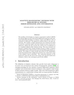
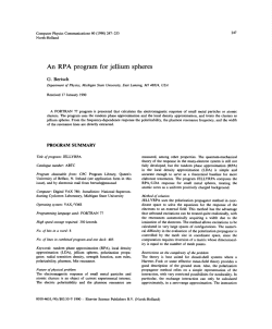
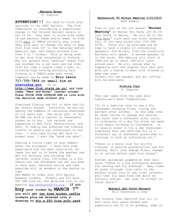
Fisheries Research 73 (2005) 323–339
Gill-net selectivity off the Portuguese western coast
Paulo Fonseca a,∗ , Rog´elia Martins a , Aida Campos a , Preciosa Sobral b
a
b
INIAP/IPIMAR, Portuguese Institute for Agriculture and Fisheries Research, Avenida de Bras´ılia, 1449-006 Lisboa, Portugal
INIAP/IPIMAR (CRIPCentro), Regional Centre for Fisheries Research, Aveiro, Canal das Pirˆamides, 3800 Aveiro, Portugal
Received 9 July 2004; received in revised form 9 January 2005; accepted 18 January 2005
Abstract
Fishing with experimental gill-nets was carried out during 1994 and 1995 off the western coast of Portugal, using mesh sizes
between 40 and 90 mm. Most sets were concentrated in the region between Set´ubal and Lisbon in shallow waters up to 100 m,
with about 1/4 being carried out at greater depths. A total of 88 species were captured over the 2 years, of which the majority
had small or no commercial value. The most important commercial species (hake, Merluccius merluccius, pouting, Trisopterus
luscus, axillary seabream, Pagellus acarne, red mullet, Mullus surmuletus, and horse mackerel, Trachurus trachurus) accounted
for about 12% of the catch weight in the 40 mm mesh panels, between 32 and 44% for mesh panels ranging between 60 and
80 mm, and 70% in the 90 mm mesh panels. The estimation of selectivity was carried out for the latter five species and also for
the dogfish, Scyliorhinus canicula, wedge sole, Dicologlossa cuneata, and spotted flounder, Citharus linguatula, applying the
SELECT method to the data pooled over both years. In the case of hake, pouting and dogfish, sufficient data were available to
estimate selectivity on a yearly basis. Four different uni-modal and a bi-modal (bi-normal) models were fitted, with the bi-normal
always providing the best fit as given by the smallest value of the ratio deviance/degrees-of-freedom. The exception was the
wedge sole where the bi-normal model did not converge and the gamma was the unimodal model providing the best fit. The
40 mm mesh panels mostly retained species of low or no commercial value and undersized hake and pouting. Mesh size panels of
60, 70 and 80 mm proved to be the most efficient in catching the commercially valuable species over the length range available,
with virtually no catch of undersized fish. The 90 mm panels retained mainly valuable species, but the overall catches were poor,
with the exception of the axillary seabream. These results highlight the difficulties of managing multispecies fisheries based only
on mesh size, since the optimal mesh varies considerably among the target species.
© 2005 Elsevier B.V. All rights reserved.
Keywords: Gill-net; Size selection; Portuguese western coast; Axillary seabream; Small-spotted dogfish; European hake; Horse mackerel;
Pouting; Striped red mullet; Spotted flounder; Wedge sole
1. Introduction
∗ Corresponding author. Tel.: +351 213 027163;
fax: +351 213 015948.
E-mail addresses: [email protected] (P. Fonseca),
[email protected] (R. Martins), [email protected] (A. Campos),
[email protected] (P. Sobral).
0165-7836/$ – see front matter © 2005 Elsevier B.V. All rights reserved.
doi:10.1016/j.fishres.2005.01.015
Most of the Portuguese fishing vessels operating in
coastal waters are included in the so-called ‘polyvalent’
(multi-gear, multi-species) fleet. This fleet consists of
almost 7000 vessels, most of them between 7 and 9 m
324
P. Fonseca et al. / Fisheries Research 73 (2005) 323–339
overall length with open-deck, and thus only fishing
within a limited area off the coastline. The economic
and social importance of this fleet is evidenced by the
contribution to the total landings and revenue, about
30 and 60%, respectively, and the number of fishermen
involved, nearly 80% of the total.1
The gears used by this fleet include gill-nets and
trammels, longlines, traps, pots, dredges, beam-trawls
and beach seines. Although most of the fishing is carried out in shallow waters, often corresponding to nursery zones, some of the fishing grounds are located at
greater depths. This is the case of longlining for the
black scabbard, Aphanopus carbo and the European
hake, Merluccius merluccius, and the gill-net and trammels fisheries for the hake and monkfish, Lophius spp.,
respectively.
Gill-nets and trammels comprise almost 50% of the
total licences issued every year (a vessel can be licensed
for the use of multiple gears). Current Portuguese legislation, Decree-law no. 7/2000 and Act 1102H/2000,
limits the use of these gears in oceanic waters by restricting fishing areas and seasons, duration of sets and
gear characteristics such as total length, and panel maximum height and mesh size.
Gill-nets are highly selective for those species captured mainly by gilling (i.e., captured behind the gillcover) or wedged (being held by a mesh around their
maximum body girth). For these, retention is supposed
to increase with size up to a length of maximum catch
and decrease thereafter, and consequently the range of
size-at-catch of a target species can be controlled with
a careful choice of the mesh size. However, in addition to mesh size, a number of technical characteristics
related to gear construction (hanging ratio) and twine
specifications (material, thickness, colour, etc.) have
a significant influence on the catch size distribution.
Similarly, biological characteristics also influence retention by size. For a number of species, the existence of
well developed teeth, protruding maxillaries, or body
projections (spines), together with higher swimming
activity, can result in a significant proportion of fish
being entangled.
While the selectivity of gill-net fisheries has been
the object of several studies in the southern coast of
Portugal (Martins et al., 1990; Santos et al., 1995, 1998,
1 Data from the General-Directorate for Fisheries and Aquaculture
(DGPA) for the year of 1995.
2003; Erzini et al., 2003), the information available for
the western coast is scarce (Martins et al., 1990). The
present study represents the first attempt to describe
gear selection patterns for a number of species caught
in the coastal waters off the western coast.
2. Materials and methods
2.1. Survey areas and gears
During 1994 and 1995, eight gill-net selectivity surveys were completed in the western coast of Portugal
from Aveiro (northwestern coast) to Sines (southwestern coast). The majority of the sets, of a total of 77, took
place in the region between Lisboa and Set´ubal (Fig. 1
and Table 1), at depths ranging from 24 to 250 m, with
most (72%) carried out in waters shallower than 100 m.
The R/V ‘Mestre Costeiro’, a 27 m overall length stern
trawler also equipped for the use of static gears, was
used for these surveys.
Fig. 1. Location of the experimental hauls. Crosses and open circles
correspond to the 1994 and 1995 sets, respectively.
P. Fonseca et al. / Fisheries Research 73 (2005) 323–339
325
Table 1
Description of the different surveys carried out in 1994 and 1995, including number of sets by survey, mesh sizes used and total fishing time
Year
Month
Nb sets
Total duration (h)
Mesh size (mm)
1994
April 19–26
June 09–29
July 06–13
November 1–16
5
12
5
6
515
40/60/70/80
40/60/70/80
40/60/70/80
40/60/70/80
1995
April 19–May 02
May 23–31
July 19–August 10
September 13–27
8
9
18
14
640
40/60/70/80/90
40/60/70/80/90
40/60/70/80/90
40/60/70/80/90
During the experiments carried out in 1994, the gear
was composed of ten panels of each mesh size, 40, 60,
70 and 80 mm stretched (nominal) length, disposed alternately, with about 30 cm spacing between adjacent
panels. In 1995 a similar number of 90 mm panels were
added to the experimental fleet. Panel dimensions were
50 m × 3 m in length and in height, respectively. Hanging coefficients were kept constant at about 0.5 (see
Table 2 for gear details).
in the morning. Although on a few occasions the fishing started before noon and lasted until the following
morning, only three sets occurred entirely during the
day. Independently of the soaking time for each set, all
mesh sizes were fished the same total time, since a single fleet was deployed with all the experimental panels
at the same time.
2.2. Experimental procedures
All species, whether commercial or not, were sorted
out by mesh size, identified to species level, sexed and
weighed to the nearest 0.1 g. Total length, as well as
opercula and maximum girth, were measured to the
nearest millimetre.
2.3. Catch handling
The most productive period for gill-net fishing is
between dusk and dawn, and therefore the gears are
normally set during the few hours before sunset and
hauled early in the morning. However, the effective
duration of fishing and deployment period is dependent on the target species and local conditions. In the
present study, the soaking time varied from about 3 to
over 24 h, either due to biological factors (occurrence
of scavengers) or operational constraints (e.g., weather
conditions preventing haul-up), with an average of 18 h
for 1994 and 13 h during 1995. Most often the fleet was
set 1 or 2 h before sunset or in the evening, and hauled
2.4. Selectivity estimation
The estimation of the selectivity of static gears,
namely gill-nets, has been the object of a number of different approaches: inference from girth measurements,
direct estimates, mortality estimates, and indirect estimates (Hamley, 1975). In the latter, the structure of
the population being fished is not known, and has to
Table 2
Technical characteristics of the gill-nets used during the different surveys
Mesh size (mm)
Length
Nb of meshes
Floatline (m)
Leadline (m)
Length
Height
40
60
70
80
90
50.7
51.8
49.3
49.5
49.7
52.3
53.2
50.8
50.8
50.8
2536
1680
1450
1270
1130
74.0
49.0
43.5
37.5
33.0
Side line (m)
Twine material
Diameter (mm)
3.0
3.0
3.0
3.0
3.0
PAmono
PAmono
PAmono
PAmono
PAmono
0.35
0.35
0.35
0.35
0.35
326
P. Fonseca et al. / Fisheries Research 73 (2005) 323–339
be inferred from the catches taken during comparative
fishing experiments that simultaneously deploy multiple gill-net panels of different mesh sizes.
Assumptions on the equal availability of fishes of all
sizes to the different mesh sizes and on the functional
form of the selection curves have to be made. A useful
simplification is to assume that selection curves of the
different mesh sizes follow the ‘principle of geometric
similarity’, introduced by Baranov (1948). According
to this assumption, the catch process is only dependent
on the relative geometry of the fish and the mesh size.
In other words, the selectivity of different mesh sizes
is equal when the ratio of fish length to mesh size is
the same. This assumption implies that all mesh sizes
are equally selective for the size of fish they catch most
efficiently (i.e., all the selection curves have the same
height). Also, the curve spread will increase proportionally with mesh size. Although the ‘principle’ is an
oversimplification of the retention process, since it does
not take into account potentially distinct fish behaviour
according to size class, or allometric growth or differences in fishing power among the different mesh size
panels, it is still the basis of most of the commonly
used methods. Other approaches have been tried, including the models used by Holt (1963) and Kirkwood
and Walker (1986) which assume that the spread of the
selection curve is the same for all mesh-sizes used.
From the early 1990s, a new methodological
approach for the analysis of gear selectivity data, the
SELECT method (Millar, 1992) has arisen. First used in
the context of trawling (Millar and Walsh, 1992), it was
then extended to static gears (Millar and Holst, 1997).
Together with the work by Fryer (1991) it constitutes a
general framework for the analysis of the selectivity of
all types of fishing gears, both at haul-level and above
(Millar and Fryer, 1999) where parameter estimation
is carried out by maximum likelihood (ML). In the
strict context of gillnet selectivity, Hovgard (1996)
and Hovgard et al. (1999) brought forward a similar
approach to selectivity parameter estimation based
on, either linear or non-linear, least squares (LS).
Although both estimation procedures may result in
very close estimates (see Erzini and Castro, 1998),
the SELECT approach carries all the advantageous
properties of maximum likelihood (e.g., unbiased and
minimum variance estimators), further allowing for
the incorporation of between-haul variability (Millar,
2000), and therefore will be used herein.
The SELECT method assumes that catches (nlj )
by length class (l) and gear size (j) follow a Poisson
distribution with parameters pj (l) (the relative fishing
intensity, a combined measure of fishing effort and
fishing power, representing the probability that a
fish of length l contacts the gear size j given that it
contacts the combined gear), λl (the abundance of
length l fish contacting the combined gear) and rj (l)
(the contact-selection curve; i.e., the probability of
retention of a fish of length l in gear size j):
nlj ≈ Pois(pj (l)λl rj (l))
(1)
For model simplification pj is usually taken as length
independent, and therefore, the log-likelihood of
expression (1) is given by:
{nlj loge pj λl rj (l) − pj λl rj (l)}
(2)
l
j
where the term not depending on any of the parameters
was excluded.
By using the proportions of the total catch (for
each length class) taken by each mesh size panels
(ylj = nlj /nl+ ), and considering that they follow a multinomial distribution with parameters nl+ and φlj =
pj rj (l)/ j pj rj (l), the model can be further reduced as
λl is eliminated from the maximization process (Millar
and Fryer, 1999). The log-likelihood of ylj can then be
written:
nlj loge (φlj )
(3)
l
j
which depends only on parameters pj and the parameters of the selection curves rj (l). For gill-net (and longline) selectivity, Millar and Holst (1997) demonstrated
that the model reduces to a log-linear model for a number of uni-modal selection curves (normal scale and
normal location, lognormal and gamma). Multimodal
models are also available under SELECT. Among these
the ‘bi-normal’ model (a mixture of two normal curves)
has often been used to accommodate a combination of
clearly different catch processes (Hovgard, 1996) or
been found to provide an overall better fit (Madsen et
al., 1999; Moth-Poulsen, 2003). These models observe
the ‘principle of geometric similarity’, with the exception of the ‘normal location’, where the selection curves
have a fixed spread.
P. Fonseca et al. / Fisheries Research 73 (2005) 323–339
A proprietary software (GILLNET, Constat, DK)
was used here for selectivity estimation (equal power
over mesh sizes was assumed). The model providing
the best fit, corresponding to the smallest value for the
ratio deviance/degrees-of-freedom, was adopted.
2.5. Comparison between selection curves
The data were too scarce for haul-by-haul selectivity estimation or even for a survey based analysis,
and therefore data from both years were pooled for
all species. However, for three of the species (pouting, Trisopterus luscus, hake, Merluccius merluccius,
and dogfish, Scyliorhinus canicula), a yearly estimation of the selectivity could be carried out. In these
cases, a likelihood ratio test (LRT) (see, for example, McCullagh and Nelder, 1989) was used to test
for significant differences in selectivity between the
2 years. For this purpose, the deviances resulting from
the fits to individual years are summed up and then
compared to the deviance resulting from the model fitted to the combined data. The combined dataset was
constructed by appending the 1995 dataset to the 1994
dataset.
The value of [deviance(1994 + 1995) − (deviance
(1994) + deviance(1995))] is distributed approximately
2 where d.f. (the degrees of freedom) is given by
χd.f.
the change in the number of parameters when fitting
the separate and the joint selection curves. The significance level was set at 0.01, that is, the difference
between years was considered statistically significant
2
if the above value exceeded χd.f.,0.01
.
3. Results
Altogether, 88 different species were captured over
the 2 years, with the number of species being higher
in 1994 (74) than in 1995 (66). This difference is most
probably related to the much more restricted geographical area surveyed during 1995. Among these, 41 species
are potentially commercialized, but most are of low
market value. Only five species can be considered economically important for this m´etier (hake, pouting, axillary seabream, Pagellus acarne, red mullet, Mullus
surmuletus, and horse mackerel, Trachurus trachurus).
The average yield (for the whole experimental fleet)
was about 31.5 kg per set, or 2.1 kg h−1 .
327
Table 3 presents the total catches by mesh size, in
number and in weight, for the most captured species,
along with the proportions of high-valued species and
total commercial species. It provides a basis for comparison among the fishing characteristics of the different mesh size panels. The 40 mm mesh panels caught
mainly low or non-commercial species, along with
small individuals of the most valuable ones. On the
other hand, for mesh sizes from 60 to 80 mm, the
proportion of highly valuable fish is within a relatively close range (0.32–0.44). Also, the proportion of
(high + low) commercial fish shows an increasing trend
with mesh size, both in number and in weight, attaining
almost one for the largest mesh size. The 90 mm panels presented the highest proportion, both in number
and in weight, of the highly valuable species (0.6 and
0.7, respectively). They retained virtually no by-catch
and caught the largest individuals of the highly valuable species. However, no direct comparisons could be
carried out with the other mesh size panels, since the
90 mm panels were only used during 1995. The exception is for the axillary seabream which was only
captured in 1995.
The most valuable species were mainly captured
within the mesh size range from 60 to 80 mm. Smaller
mesh sizes (40 mm) were observed to catch a high proportion of undersized fish, while the largest mesh size
(90 mm) retained mainly valuable species, but had considerably lower yields.
3.1. Length frequency distributions
The length frequency distributions for the species
analyzed are shown in Fig. 2(a)–(n). These plots correspond to the cases where the estimation of selection
curves was possible. Hake, pouting and dogfish were
the only species for which there was enough data for
an analysis by year.
Wedge sole, Dicologlossa cuneata, and spotted
flounder, Citharus linguatula, were captured within
approximately the same length range with similar single modes (Fig. 2(a) and (b)). The former was captured
almost exclusively above its minimum landing size
(MLS) of 15 cm. The red mullet was always captured
above the MLS (15 cm), its size distribution being
multi-modal and denoting a sharp selection by the
different mesh size panels (Fig. 2(c)). The majority of
the axillary seabreams were concentrated within the
328
P. Fonseca et al. / Fisheries Research 73 (2005) 323–339
Table 3
Catches in number (a) and weight (kg) (b) for high, low and non commercially valuable species, by mesh size
Catch/mesh size
40
60
70
80
90a
(a) High commercial value
European hake
Axillary seabream
Red mullet
Pouting
Horse mackerel
142
6
46
229
229
260
192
83
670
153
254
256
77
390
48
156
285
41
135
20
55
218
4
17
2
Low commercial value
Wedge sole
Dogfish
Other
203
111
4079
73
701
1186
24
1033
1379
9
926
1187
41
141
Non commercial
Spotted flounder
Other
174
1132
349
323
111
148
41
98
5
54
Proportion of high commercial value
Proportion of commercial value
(b) High commercial value
European hake
Axillary seabream
Red mullet
Pouting
Horse mackerel
Low commercial value
Wedge sole
Dogfish
Other
Non commercial
Spotted flounder
Other
Proportion of high commercial value
Proportion of commercial value
a
0.11
0.78
0.42
0.79
0.39
0.90
0.32
0.93
0.60
0.88
21
1
3
12
16
89
33
15
90
24
131
64
25
72
9
94
94
16
32
4
32
90
1
5
0
9
13
304
5
157
259
2
424
513
1
428
500
18
47
6
75
15
46
6
26
2
14
0
7
0.12
0.81
0.44
0.89
0.36
0.96
0.32
0.98
0.70
0.96
90 mm nets were only used in 1995.
range of 21–31 cm, thus above the MLS of 18 cm; two
relatively close modes of similar importance can be
perceived, one at 25 and the other at 30 cm (Fig. 2(d)).
Similarly, practically no horse mackerel below the
MLS (15 cm) were caught, but the catch length
distribution is distinctly broken in two (Fig. 2(e)),
with the individuals from 16 to 20 cm corresponding
basically to those retained by the 40 mm mesh panels,
and those from 22 to about 32 cm, with modes at 16
and 26 cm, respectively.
Hake catches varied from 19 to 67 cm in length,
with most fish concentrated in the range of 21–51 cm
(Fig. 2(f)–(h)). Individuals below the MLS (27 cm)
were caught in considerable numbers in the 1994 sets.
They were mostly captured in the 40 mm mesh panels,
with about 84% of the catch constituted by undersized
fish, whereas for 60–80 mm panels this percentage was
at the most about 5%. For pouting, a bi-modal distribution clearly split at the MLS (17 cm) can be observed
(Fig. 2(i)). Undersized individuals (71% of the total)
were exclusively retained by the smallest mesh size
and presented a mode at 15 cm, while for commercially
sized catches the mode is situated at 23 cm. The dogfish, ranging in size from 21 to 71 cm, were caught with
a mode at 50 cm, but the most abundant length classes
were within the range of 38–55 cm (Fig. 2(l)).
P. Fonseca et al. / Fisheries Research 73 (2005) 323–339
329
Fig. 2. Length frequency distributions by mesh size of the different species under analysis (a) spotted flounder; (b) wedge sole; (c) red mullet; (d)
axillary seabream; (e) horse mackerel; (f–h) hake (pooled, 1994 and 1995); (i–k) pouting (pooled, 1994 and 1995); (l–n) small spotted dogfish
(pooled, 1994 and 1995). Patterns: crossed hatched, 40 mm mesh panels; white, 60 mm; dotted, 70 mm, horizontal hatched, 80 mm; grey, 90 mm;
and thick line, pooled.
330
P. Fonseca et al. / Fisheries Research 73 (2005) 323–339
Fig. 2. (Continued ).
3.2. Selectivity estimation
Table 4 displays the results of the fits for the four
uni-modal and the single bi-modal (bi-normal) models, while the modal lengths and spread values of the
selection curves corresponding to the best-fit model
are shown in Table 5. For the majority of the datasets
the bi-normal model provided the best fit, presenting
the smallest value for the ratio deviance/d.f. The exception was for the wedge sole where no convergence
could be obtained and the Gamma presented the best
fit among the unimodal models. In all of the bi-normal
fits, the two modes of the fitted bi-normal curves were
insufficiently separated to appear as two separate peaks
in selection probability (Fig. 3). Instead, the fitted binormal curves were all uni-modal with varying degrees
of right-skewness.
Both flatfish species (spotted flounder and wedge
sole) were caught approximately within the same
length range, attaining a maximum size of 30 cm.
P. Fonseca et al. / Fisheries Research 73 (2005) 323–339
331
Table 4
Selection curves parameters estimates resulting from the use of four uni-modal and one bi-modal models, with the corresponding deviances,
degrees of freedom and p-values, for the different species under study
Species
Year
Model
Spotted flounder
1994 + 1995
Normal location
Normal scale
Gamma
Log normal
Bi-normal
Fixed spread
Spread α mj
Spread α mj
Spread α mj
Spread α mj
Wedge sole
1994
Normal location
Normal scale
Gamma
Log normal
Bi-normal
Fixed spread
Spread α mj
Spread α mj
Spread α mj
Spread α mj
Red mullet
1994 + 1995
Normal location
Normal scale
Gamma
Log normal
Bi-normal
Fixed spread
Spread α mj
Spread α mj
Spread α mj
Spread α mj
Axillary seabream
1995
Normal location
Normal scale
Gamma
Log normal
Bi-normal
Fixed spread
Spread α mj
Spread α mj
Spread α mj
Spread α mj
Horse mackerel
1994 + 1995
Normal location
Normal scale
Gamma
Log normal
Bi-normal
Fixed spread
Spread α mj
Spread α mj
Spread α mj
Spread α mj
Hake
1994 + 1995
Normal location
Normal scale
Gamma
Log normal
Bi-normal
Fixed spread
Spread α mj
Spread α mj
Spread α mj
Spread α mj
1994
Normal location
Normal scale
Gamma
Log normal
Bi-normal
Fixed spread
Spread α mj
Spread α mj
Spread α mj
Spread α mj
1995
Normal location
Normal scale
Gamma
Log normal
Bi-normal
Fixed spread
Spread α mj
Spread α mj
Spread α mj
Spread α mj
1994 + 1995
Normal location
Normal scale
Gamma
Log normal
Bi-normal
Fixed spread
Spread α mj
Spread α mj
Spread α mj
Spread α mj
1994
Normal location
Normal scale
Gamma
Log normal
Bi-normal
Fixed spread
Spread α mj
Spread α mj
Spread α mj
Spread α mj
1995
Normal location
Normal scale
Gamma
Log normal
Bi-normal
Fixed spread
Spread α mj
Spread α mj
Spread α mj
Spread α mj
Pouting
d.f.
p-value
Mesh sizes
(k, σ) = (0.332, 3.045)
(k1 , k2 ) = (0.354, 0.057)
(α, k) = (0.010, 37.270)
(µ1 , σ) = (2.612, 0.168)
(k1 , k2 , k3 , k4 , c) = (0.338,
0.034, 0.378, 0.091, 0.308)
(k, σ) = (0.409, 4.135)
(k, k2 ) = (0.426, 0.072)
(α, k) = (0.015, 29.795)
µ1 , σ) = (2.851, 0.196)
No convergence
Parameters
Deviance
34.24
40.99
33.27
32.07
21.23
22
22
22
22
19
0.0464
0.0083
0.0581
0.0762
0.3240
40, 60, 70
40, 60, 70
40, 60, 70
40, 60, 70
40, 60, 70
22.47
18.56
17.20
17.77
–
24
24
24
24
–
0.5512
0.7751
0.8399
0.8140
–
40, 60, 70
40, 60, 70
40, 60, 70
40, 60, 70
40, 60, 70
(k, σ) = (0.412, 2.507)
(k1 , k2 ) = (0.423, 0.040)
(α, k) = (0.004, 102.639)
(µ1 , σ) = (2.823, 0101)
(k1 , k2 , k3 , k4 , c) = (0.404,
0.014, 0.430, 0.047, 0.582)
(k, σ) = (0.355, 2.684)
(k1 , k2 ) = (0.362, 0.037)
(α, k) = (0.004, 96.583)
(µ1 , σ) = (3.075, 0.102)
(k1 , k2 , k3 , k4 , c) = (0.354,
0.027, 0.395, 0.057, 0.171)
(k, σ) = (0.477, 5.027)
(k1 , k2 ) = (0.507, 0.091)
(α, k) = (0.020, 25.816)
(µ1 , σ) = (3.004, 0.211)
(k1 , k2 , k3 , k4 , c) = (0.473,
0.045, 0.580, 0.166, 0.212)
(k, σ) = (0.559, 7.177)
(k1 , k2 ) = (0.592, 0.113)
(α, k) = (0.023, 25.510)
(µ1 , σ) = (3.152, 0.206)
(k1 , k2 , k3 , k4 , c) = (0.576,
0.057, 0.599, 0.161, 0.409)
(k, σ) = (0.589,7.238)
(k1 , k2 ) = (0.621, 0.117)
(α, k) = (0.024, 25.510)
(µ1 , σ) = (3.200, 0.207)
(k1 , k2 , k3 , k4 , c) = (0.596,
0.066, 0.646, 0.185, 0.278)
(k, σ) = (0.554, 7.082)
(k1 , k2 ) = (0.584, 0.107)
(α, k) = (0.022, 26.974)
(µ1 , σ) = (3.141, 0.202)
(k1 , k2 , k3 , k4 , c) = (0.577,
0.053,0.142, 0.142, 0.502)
(k, σ) = (0.376, 2.871)
(k1 , k2 ) = (0.394, 0.050)
(α, k) = (0.006, 61.567)
(µ1 , σ) = (2.748, 0.129)
(k1 , k2 , k3 , k4 , c) = (0.377,
0.035, 0.434, 0.074, 0.165)
(k, σ) = (0.368, 2.866)
(k1 , k2 ) = (0.387, 0.050)
(α, k) = (0.007, 59.508)
(µ1 , σ) = (2.730, 0.131)
(k1 , k2 , k3 , k4 , c) = (0.362,
0.032, 0.427, 0.062, 0.324)
(k, σ) = (0.382, 2.875)
(k1 , k2 ) = (0.399, 0.050)
(α, k) = (0.006, 61.996)
(µ1 , σ) = (2.759, 0.129)
(k1 , k2 , k3 , k4 , c) = (0.386,
0.038, 0.464, 0.105, 0.042)
53.32
53.81
56.22
58.58
40.38
58
58
58
58
55
0.6498
0.6319
0.5418
0.4541
0.9300
40, 60, 70, 80
40, 60, 70, 80
40, 60, 70, 80
40, 60, 70, 80
40, 60, 70, 80
95.70
131.88
108.36
100.33
66.70
61
61
61
61
58
0.0030
0.0000
0.0002
0.0011
0.2027
60, 70, 80, 90
60, 70, 80, 90
60, 70, 80, 90
60, 70, 80, 90
60, 70, 80, 90
100.99
104.41
99.75
102.62
71.77
50
50
50
50
47
0.0000
0.0000
0.0000
0.0000
0.0115
40, 60, 70
40, 60, 70
40, 60, 70
40, 60, 70
40, 60, 70
290.64
221.06
225.96
240.73
168.96
130
130
130
130
127
0.0000
0.0000
0.0000
0.0000
0.0076
40, 60, 70, 80
40, 60, 70, 80
40, 60, 70, 80
40, 60, 70, 80
40, 60, 70, 80
188.77
160.56
158.00
163.59
129.77
118
118
118
118
115
0.0000
0.0056
0.0082
0.0035
0.1639
40, 60, 70, 80
40, 60, 70, 80
40, 60, 70, 80
40, 60, 70, 80
40, 60, 70, 80
166.27
120.61
133.08
143.37
105.74
112
112
112
112
109
0.0007
0.2725
0.0850
0.0244
0.5707
40, 60, 70, 80
40, 60, 70, 80
40, 60, 70, 80
40, 60, 70, 80
40, 60, 70, 80
117.14
151.79
110.31
99.65
68.19
73
73
73
73
70
0.0008
0.0000
0.0032
0.0208
0.5389
40, 60, 70, 80
40, 60, 70, 80
40, 60, 70, 80
40, 60, 70, 80
40, 60, 70, 80
47.16
71.20
55.01
49.33
35.34
58
58
58
58
55
0.8448
0.1049
0.5871
0.7843
0.9819
40, 60, 70, 80
40, 60, 70, 80
40, 60, 70, 80
40, 60, 70, 80
40, 60, 70, 80
105.25
124.06
99.26
94.10
62.51
67
67
67
67
64
0.0020
0.0000
0.0064
0.0162
0.5292
40, 60, 70, 80
40, 60, 70, 80
40, 60, 70, 80
40, 60, 70, 80
40, 60, 70, 80
332
P. Fonseca et al. / Fisheries Research 73 (2005) 323–339
Table 4 (Continued )
Species
Year
Model
Dogfish
1994 + 1995
Normal location
Normal scale
Gamma
Log normal
Bi-normal
Fixed spread
Spread α mj
Spread α mj
Spread α mj
Spread α mj
1994
Normal location
Normal scale
Gamma
Log normal
Bi-normal
Fixed spread
Spread α mj
Spread α mj
Spread α mj
Spread α mj
1995
Normal location
Normal scale
Gamma
Log normal
Bi-normal
Fixed spread
Spread α mj
Spread α mj
Spread α mj
Spread α mj
Parameters
Deviance
d.f.
p-value
Mesh sizes
(k, σ) = (0.680, 5.952)
(k1 , k2 ) = (0.699, 0.095)
(α, k) = (0.012, 56.893)
(µ1 , σ) = (3.328, 0.133)
(k1 , k2 , k3 , k4 , c) = (0.694,
0.083, 0.856, 0.225, 0.026)
(k, σ) = (0.680, 6.017)
(k1 , k2 ) = (0.695, 0.097)
(α, k) = (0.012, 57.209)
(µ1 , σ) = (3.325, 0.131)
(k1 , k2 , k3 , k4 , c) = (0.695,
0.085, 1.239, 0.472, 0.006)
(k, σ) = (0.679, 5.931)
(k1 , k2 ) = (0.708, 0.100)
(α, k) = (0.014, 50.355)
(µ1 , σ) = (3.339, 0.142)
(k1 , k2 , k3 , k4 , c) = (0.669,
0.064, 0.784, 0.128, 0.365)
309.10
363.52
283.31
263.37
199.60
127
127
127
127
124
0.0000
0.0000
0.0000
0.0000
0.0010
40, 60, 70, 80
40, 60, 70, 80
40, 60, 70, 80
40, 60, 70, 80
40, 60, 70, 80
257.15
312.10
235.21
211.55
142.63
109
109
109
109
106
0.0000
0.0000
0.0000
0.0000
0.0102
40, 60, 70, 80
40, 60, 70, 80
40, 60, 70, 80
40, 60, 70, 80
40, 60, 70, 80
160.51
187.55
164.13
159.49
130.65
112
112
112
112
109
0.0018
0.0000
0.0010
0.0022
0.0773
40, 60, 70, 80
40, 60, 70, 80
40, 60, 70, 80
40, 60, 70, 80
40, 60, 70, 80
Table 5
Modal length and spread, by mesh size, for the best-fit model of table 4
Species
Year
Model
Mesh size
Modal lengtha
Spreada
Spotted flounder
1994 + 1995
Bi-normal
40
60
70
13.5
20.3
23.7
1.37
2.06
2.40
Wedge sole
1994
Gamma
40
60
70
16.8
25.2
29.4
3.13
4.69
5.47
Red mullet
1994 + 1995
Bi-normal
40
60
70
80
16.1
24.2
28.3
32.3
0.55
0.83
0.97
1.11
Axillary seabream
1995
Bi-normal
60
70
80
90
21.3
24.8
28.3
31.9
1.61
1.88
2.15
2.41
Horse mackerel
1994 + 1995
Bi-normal
40
60
70
18.9
28.4
33.1
1.82
2.72
3.18
Hake
1994 + 1995
Bi-normal
40
60
70
80
23.0
34.6
40.3
46.1
2.26
3.39
3.96
4.52
1994
Bi-normal
40
60
70
80
23.9
35.8
41.7
47.7
2.63
3.94
4.60
5.26
1995
Bi-normal
40
60
70
80
23.1
34.6
40.4
46.2
2.12
3.18
3.71
4.24
P. Fonseca et al. / Fisheries Research 73 (2005) 323–339
333
Table 5 (Continued )
Species
Year
Model
Mesh size
Modal lengtha
Spreada
Pouting
1994 + 1995
Bi-normal
40
60
70
80
15.1
22.6
26.4
30.2
1.41
2.12
2.47
2.83
1994
Bi-normal
40
60
70
80
14.5
21.7
25.4
29.0
1.29
1.94
2.27
2.59
1995
Bi-normal
40
60
70
80
15.4
23.2
27.0
30.9
1.52
2.28
2.66
3.05
1994 + 1995
Bi-normal
40
60
70
80
27.8
41.7
48.6
55.6
3.30
4.95
5.78
6.60
1994
Bi-normal
40
60
70
80
27.8
41.7
48.7
55.6
3.40
5.10
5.94
6.79
1995
Bi-normal
40
60
70
80
26.8
40.1
46.8
53.5
2.54
3.81
4.45
5.08
Dogfish
a
For the bi-normal model data corresponds to the curve associated with the primary mode.
However, their selection curves are considerably different. For spotted flounder, the best fit was provided by
the bi-normal model (Fig. 3(a)), while for wedge sole
the Gamma model fitted better (Fig. 3(b)). The former
species systematically displayed smaller modal lengths
(13.5, 20.3 and 23.7 cm) than the latter (16.8, 25.2 and
29.4 cm) and smaller spreads (1.37, 2.06, 2.40 cm versus 3.13, 4.69, 5.47 cm), for the 40, 60 and 70 mm
mesh sizes, respectively. The analysis of Fig. 3(a) and
Fig. 2(a) together suggests that an intermediate mesh
size between 40 and 60 mm would be the most effective for the capture of the spotted flounder. For wedge
sole (Fig. 3(b)), the most captured size class coincides
with the modal length of the 40 mm mesh size panels.
For the red mullet, as mentioned above, the differences in size distribution by mesh size were more
evident, with clear modes and narrow intervals. As a
consequence, the bi-normal selection curves (Fig. 3(c))
appear very narrow. Modal lengths for the 40–80 mm
mesh size panels varied from 16.1 to 32.3 cm. Although
all mesh sizes only caught commercially sized individuals, the 70 mm panels were more efficient at catching the bigger fish of the available length range, while
catches in the 80 mm panels were much lower due to
scarcity of fish above 30 cm. The axillary seabream was
the only species with sufficiently high catches in the
90 mm mesh panels to allow selectivity estimation for
this mesh size (Fig. 3(d)). Modal lengths in the 60, 70,
80 and 90 mm mesh sizes, using the bi-normal model,
were 21.3, 24.8, 28.3 and 31.9 cm, respectively. The
catch of undersized fish was negligible and restricted
to the 60 mm panels. Although the 70 and 80 mm panels were the most efficient, by number, if catches are
analysed by weight then both the 80 and 90 mm had
similar yields. For horse mackerel, bi-modal selection
curves estimated for 40, 60 and 70 mesh size panels presented modal lengths of 18.9, 28.4 and 33.1 cm, respectively (Fig. 3(e)). Hake selectivity was estimated for
both years (Fig. 3(f)–(h)) by fitting a bi-normal model
to the 40, 60, 70 and 80 mm panels. Modal lengths of
334
P. Fonseca et al. / Fisheries Research 73 (2005) 323–339
Fig. 3. Selection curves by mesh size for the different species under analysis (a) spotted flounder; (b) wedge sole; (c) red mullet; (d) axillary
seabream; (e) horse mackerel; (f–h) hake (pooled, 1994 and 1995); (i–k) pouting (pooled, 1994 and 1995); (l–n) small spotted dogfish (pooled,
1994 and 1995). Line patterns: dashed/dotted, 40 mm; dotted, 60 mm; thin, 70 mm; thick, 80 mm; and dashed, 90 mm.
P. Fonseca et al. / Fisheries Research 73 (2005) 323–339
335
Fig. 3. (Continued ).
23.9, 35.8, 41.7 and 47.7 were found for 1994 while
those for the following year were only slightly smaller,
23.1, 34.6, 40.4 and 46.2 cm. Looking at Fig. 3(f) and
Fig. 2(f) jointly, where selection curves and catches for
pooled data are displayed, it is noticeable that the 60
and 70 mm panels are the most efficient, retaining approximately the same numbers of individuals, although
the latter catches a higher proportion of bigger (more
valuable) fish. Comparison of the estimated selection
curves by the LRT test (p = 0.0466) leads to the conclu-
sion that no statistically significant differences could be
found in gear selectivity for both years.
For pouting, selection curves in 1994 and 1995
were estimated over the same range of mesh sizes,
40–80 mm, with the bi-normal model (Fig. 3(i)–(k)).
Modal lengths were lower in the first year (14.5, 21.7,
25.4 and 29.0 cm versus 15.4, 23.2, 27.0 and 30.9 cm),
and the curves presented a clear right-skewness.
The 60 mm mesh panels were the most efficient in
retaining the fish within the size range available,
336
P. Fonseca et al. / Fisheries Research 73 (2005) 323–339
without catching undersized individuals. The LRT test
indicated a significant difference (p < 0.01) in gear
selectivity between 1994 and 1995.
Similarly to hake and pouting, both yearly and
pooled datasets for dogfish were best fitted by a binormal model (Fig. 3(l)–(n)). In 1994, modal lengths
were 27.8, 41.7, 48.7 and 55.6 cm for the 40–80 mm
mesh size panels. In the following year, when smaller
fish were caught, slightly lower values were obtained
(26.8, 40.1, 46.8 and 53.5 cm). Differences in selectivity between both years were statistically significant
(p < 0.01).
4. Discussion and conclusions
Previous results had already been obtained for some
of the species analysed within this study, both in the
Portuguese coast (Martins et al., 1990; Santos et al.,
2003; Erzini et al., 2003) and in Greek waters (Petrakis
and Stergiou, 1995, 1996; Stergiou and Erzini, 2002)
(Table 6). However, not only the methods of estimating the selectivity parameters varied among experiments, but the estimation was always carried out over
pooled datasets. In such conditions the difficulty of
distinguishing between real differences in selectivity
and method-induced results is aggravated by the potential masking of between-set variability. For the axillary
seabream and the hake (in Portuguese southern waters)
and the red mullet (in Greek waters), the SELECT approach had previously been used in recent studies, thus
providing a more reliable basis for comparison. A good
agreement in the selectivity estimates was found for
the hake, where an almost total coincidence in both the
operational condition (mesh size range) and modelling
(bi-normal model) took place. Conversely, for the axillary seabream the modal lengths previously estimated
are higher than those of the present study, for an almost
coincident range of mesh sizes, and so are those for red
mullet in Greek waters, although here the overlap of
mesh sizes is very restricted.
With the exception of the 40 mm mesh panels, where
the majority of hake and pouting catch was below the
MLS, no undersized fish was caught. If the selection
factors2 (SF = L50 /m) are estimated and compared with
2 For gill-nets, the length of 50% retention was calculated on the
ascending arm of the curve; m is the stretched mesh size.
those from trawls using 65 mm, or larger, diamond and
square mesh codends (Table 7), it can be concluded
that gill-nets of similar mesh size are much more selective. Actually, the SF values are equal or even larger
than those found for square mesh codends. A further
advantage of gill-nets is that by a careful choice of the
mesh size it is not only possible to tackle the problem of
catch of undersized fish, but also to control the catch of
bigger fish in situations where recruitment overfishing
is at issue.
From the catch (in weight) of the most important
commercial species (Table 3(b)), it is noticeable that
the mesh size providing the best yields varied according to the species. Pouting and horse mackerel were
preferentially retained by the 60 mm mesh size panels,
which is in line with the current Portuguese legislation that enforces the use of a mesh size in the range
of 60–79 mm for fisheries targeting these species. For
the red mullet and the axillary seabream, also caught by
the same mesh size range, the best yields were observed
in the 70 and 80 mm nets, respectively. Therefore, for
the latter species, the use of mesh sizes smaller than
80 mm will result in catches constituted by smaller and
less valuable fish. In contrast, for hake the 70 mm nets
proved to be the most efficient, catching about 47 and
40% more than the 60 and 80 mm nets, respectively.
The legislation enforces the use of a minimum mesh
size equal or higher than 80 mm, which is justifiable
since the length at first maturity for females is 45.3 cm
(Cardador et al., 2000), and therefore a smaller mesh
size would retain a large quantity of immature individuals. The comparative yields of different mesh size
panels will depend on the size distribution of the population fished. However, the catches in the present study
were pooled over different seasons and two consecutive years, and therefore should closely reflect the size
range captured by the commercial boats.
Overall, gill-nets from 60 to 80 mm mesh size seem
to be the most adequate for the correct management of
the majority of the species targeted by these gears. According to the present study, the discards of undersized
and/or immature individuals would be small when using these mesh sizes, consisting mainly of low commercial value species or damaged fish resulting from
an excessive set duration, e.g., by consumption by other
fish and scavenging amphipods. Due to the selectivity
of these gears, fishermen can easily adapt mesh size
(within the legal framework) to specific target species
Table 6
Comparative results among the selection data obtained during the present study and those from former studies carried out in Portuguese and Mediterranean waters for common
species
Species
Region
Date
Length
range (cm)
Selection method/model
Mesh sizeb
(mm)
Modal
length (cm)
Spread
(cm)
Pouting
North Portugal
1990
13–34
HOLT/normal
40
60
80
15.3
20.5
28.2
4.26
Reference
Martins et al. (1990)
West coast, PT
1994/1995
11–35
SELECT/bi-normal
40
60
70
80
15.1
22.6
26.4
30.2
1.41
2.12
2.47
2.83
Present study
Axillary seabream
South Portugal
1997/1998
13–34
SELECT/normal scale
60
70
80
23.1
27.0
30.8
2.73
3.19
3.64
Erzini et al. (2003)
Axillary seabream
Aegean sea (Greek waters)
1992/1993
10–23a
HOLT/normal
42
46
15.4a
16.9a
1.08
Petrakis and Stergiou (1996)
Axillary seabream
West coast, PT
1994/1995
16–36
SELECT/bi-normal
60
70
80
90
21.3
24.8
28.3
31.9
1.61
1.88
2.15
2.41
Present study
Red mullet
Aegean sea (Greek waters)
1992/1993
11–23a
HOLT/normal
38
42
46
15.4a
17.1a
18.8a
1.05
Petrakis and Stergiou (1995)
Red mullet
Cyclades Aegean sea (Greek waters)
1997/1998
12–30
SELECT/log-normal
44
48
20.2
22.0
2.24
2.44
Stergiou and Erzini (2002)
Red mullet
West coast, PT
1994/1995
16–38
SELECT/bi-normal
40
60
70
80
16.1
24.2
28.3
32.3
0.55
0.83
0.97
1.11
Present study
Hake
South Portugal
1999/2002
17–65
SELECT/bi-normal
70
80
90
40.1
46.7
51.0
2.42
2.82
3.08
Santos et al. (2003)
Hake
West coast, PT
1994/1995
19–67
SELECT/bi-normal
40
60
70
80
23.0
34.6
40.3
46.1
2.26
3.39
3.96
4.52
Present study
P. Fonseca et al. / Fisheries Research 73 (2005) 323–339
Pouting
Existing estimates derived by theoretical methods were omitted.
a Total length converted from fork stretched mesh length using relationships by Moutopoulos and Stergiou (2002).
b Stretched mesh.
337
338
P. Fonseca et al. / Fisheries Research 73 (2005) 323–339
Table 7
Comparison between the selection factors derived for gill-nets in the
present study and those from codend selectivity experiments for a
subset of common species
The insightful comments by one of the referees were
of extreme value during the revision process. The
work was carried out under the scope of the research
project BIOECO/93/02 partially subsidized by the
EU/DGFISH.
Gill-nets
Trawls
4.2
2.0–2.3 (65–80d)
3.5–4.3 (65s)
Axillary seabreama
3.2
1.8 (80d)
3.1 (65s)
References
Poutingc
3.3
3.4 (65s)
Hakea,b
5.0
2.3–3.0 (65–80d)
3.9–5.1 (65s)
Red mulletc
3.8
3.5 (65s)
Baranov, F.I., 1948. Theory and assessment of fishing gear: theory
of fishing with gill-nets, Chapter 7. Pishchepromizdat, Moscow
(Translated from Russian by the Ontario Department of Lands
and Forest, Maple, Ont.).
Campos, A., Fonseca, P., 2003. Selectivity of diamond and square
mesh cod ends for horse mackerel (Trachurus trachurus), European hake (Merluccius merluccius) and axillary seabream (Pagellus acarne) in the shallow groundfish assemblage off the southwest coast of Portugal. Sci. Mar. 67, 249–260.
Campos, A., Fonseca, P., Henriques, V., 2003. Size selectivity for
four species of the deep groundfish assemblage off the Portuguese
southwest coast: evidence of mesh size, mesh configuration and
cod end catch effects. Fish. Res. 63, 213–233.
Cardador, F., Morgado, C., L´ucio, P., Pi˜nero, C., Sainza, M., Santurtun, M., 2000. New maturity ogive for the southern stock
of hake (ICES Divisions VIIIc+IXa). Int. Coun. Explor. Sea
2000/ACFM:04.
Erzini, K., Castro, M., 1998. An alternative methodology for fitting selectivity curves to pre-defined distributions. Fish. Res. 34,
307–313.
Erzini, K., Gonc¸alves, J.M.S., Bentes, L., Lino, P.G., Ribeiro, J.,
Stergiou, K.I., 2003. Quantifying the roles of competing static
gears: comparative selectivity of longlines and monofilament gill
nets in a multi-species fishery of the Algarve (southern Portugal).
Sci. Mar. 67, 341–352.
Fryer, R.J., 1991. A model of between-haul variation in selectivity.
ICES J. Mar. Sci. 48, 281–290.
Hamley, J.M., 1975. Review of gill-net selectivity. J. Fish. Res. Board
Can. 32, 1943–1969.
Hovgard, H., 1996. A two-step approach to estimating selectivity
and fishing power of research gill nets used in Greenland. Can.
J. Fish. Aquat. Sci. 53, 1007–1013.
Hovgard, H., Lassen, H., Madsen, N., Moth-Poulsen, T., Wileman,
D., 1999. Gill-net selectivity for North Sea Atlantic cod (Gadus
morhua): model ambiguity and data quality are related. Can. J.
Fish. Aquat. Sci. 56, 1307–1316.
Holt, S.J., 1963. A method for determining gear selectivity and its
application. ICNAF Spec. Publ. 5, 106–115.
Kirkwood, G.P., Walker, T.I., 1986. Gill-net mesh selectivities for
gummy shark, Mustelus antarcticus Gunther, taken in Southeastern Australian waters. Aust. J. Mar. Freshwater Res. 37,
697–698.
Madsen, N., Holst, R., Wileman, D., Moth-Poulsen, T., 1999. Size
selectivity of sole gill nets fished in the North Sea. Fish. Res. 44,
59–73.
Martins, R., Cardador, F., Sobral, M., 1990. Gill-net selectivity experiments on pout (Trisopterus luscus) in Portuguese waters. Int.
Horse
mackerela,b
In parentheses: the codend mesh size range and mesh shape (s:
square, d: diamond).
a Campos and Fonseca (2003).
b Campos et al. (2003).
c Mendes et al. (2004).
and to changes in the population size structure. There is
apparently little incentive to adopt illegal mesh sizes, in
contrast to what happens with trawling, since it does not
pay to use smaller mesh sizes which will catch smaller
and less valuable fish, at the risk of loosing larger and
higher priced individuals.
Notwithstanding, gill-net m´etiers constitute a major
source of concern for stock management, due to the difficulty of enforcing the compliance with the maximum
length of gears, which should be related with vessel
length, and of effective fishing time, that should not
exceed 24 h. Consequently, the key management problem is the determination of the fishing effort exerted by
these gears that is largely unknown and uncontrolled.
Acknowledgements
The authors would like to express their recognition
to all those participating in the sea trials, particularly
to Manuel Barata whose expertise was fundamental
in preparing the experimental gear; to Prof. Karim
Erzini (University of the Algarve, PT) for his thorough
revision of the first and final manuscripts; to Prof.
Russell B. Millar (University of Auckland, NZ) for
advice on the statistical comparison of selection curves
and comments on the second manuscript, and to Dr.
Peter A.M. Stewart for reviewing the final manuscript.
P. Fonseca et al. / Fisheries Research 73 (2005) 323–339
Coun. Explor. Sea, Fish Capture Committee, C.M. 1990/B:26,
Session U.
McCullagh, P., Nelder, J.A., 1989. Generalized linear models. In:
Monographs on Statistics and Applied Probability, vol. 37, second ed. Chapman & Hall, London, 511 pp.
Mendes, B., Fonseca, P., Campos, A., 2004. Selectividade em sacos
de redes de arrasto para seis esp´ecies de peixes na costa sudoeste Portuguesa. Relat. Cient. T´ec. IPIMAR. S´erie Digital
(http://www.ipimar-iniap.ipimar.pt) no. 11, 19 pp. (in Portuguese
with an English abstract).
Millar, R.B., 1992. Estimating the size-selectivity of fishing gear by
conditioning on the total catch. J. Am. Stat. Assoc. 87, 962–968.
Millar, R.B., 2000. Untangling the confusion surrounding the estimation of gillnet selectivity. Can. J. Fish Aquat. Sci. 57, 507–
511.
Millar, R.B., Walsh, S.J., 1992. Analysis of trawl selectivity studies
with an application to trouser trawls. Fish. Res. 13, 205–220.
Millar, R.B., Holst, R., 1997. Estimation of gill-net and hook selectivity using log-linear models. ICES J. Mar. Sci. 54, 471–477.
Millar, R.B., Fryer, R.J., 1999. Estimating the size-selection curves
of towed gears, traps, nets and hooks. Rev. Fish Biol. Fish. 9,
89–116.
Moth-Poulsen, T., 2003. Seasonal variations in selectivity of plaice
trammel nets. Fish. Res. 61, 87–94.
339
Moutopoulos, D.K., Stergiou, K.I., 2002. Length–weight and
length–length relationships of fish species from Aegean Sea
(Greece). J. Appl. Ichthyol. 18, 200–203.
Petrakis, G., Stergiou, K.I., 1995. Gill net selectivity for Diplodus
annularis and Mullus surmuletus in Greek waters. Fish. Res. 21,
455–464.
Petrakis, G., Stergiou, K.I., 1996. Gill net selectivity for four species
(Mullus barbatus, Pagellus erythrinus, Pagellus acarne and
Spicara flexuosa) in Greek waters. Fish. Res. 27, 17–27.
Santos, M.N., Monteiro, C.C., Erzini, K., 1995. Aspects of the biology and gill-net selectivity of the axillary seabream (Pagellus
acarne, Risso) and common Pandora (Pagellus erythrinus, Linnaeus) from the Algarve (south Portugal). Fish. Res. 23, 223–236.
Santos, M.N., Monteiro, C.C., Erzini, K., Lasserre, G., 1998. Maturation and gill-net selectivity of two small seabreams (genus
Diplodus) from the Algarve coast (south Portugal). Fish. Res.
36, 185–194.
Santos, M.N., Gaspar, M., Monteiro, C.C., Erzini, K., 2003. Gillnet selectivity for European hake Merluccius merluccius from
southern Portugal: implications for fishery management. Fish.
Sci. 69, 873–882.
Stergiou, K.I., Erzini, K., 2002. Comparative fixed gear studies in the
Cyclades (Aegean Sea): size selectivity of small-hook longlines
and monofilament gill nets. Fish. Res. 58, 25–40.