1. Art and Diseño

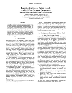
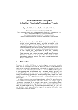
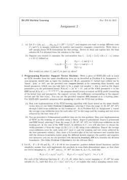
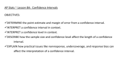
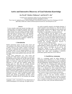
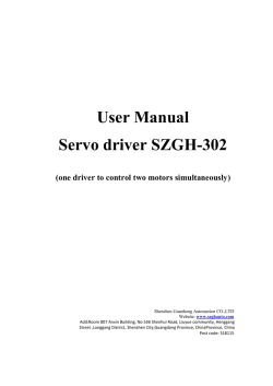
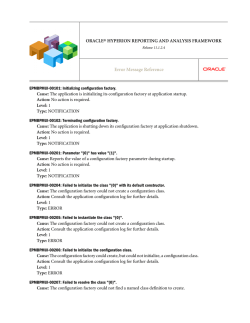
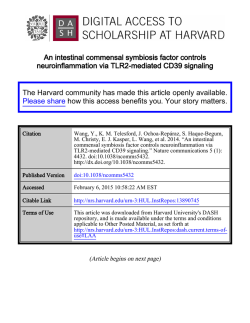
Case-Based Parameter Selection for Plans:
Coordinating Autonomous Vehicle Teams
Bryan Auslander1 , Tom Apker2 , and David W. Aha3
1
Knexus Research Corporation; Springfield VA; USA
2
Exelis Inc.; Alexandria VA; USA
3
Navy Center for Applied Research in Artificial Intelligence;
Naval Research Laboratory (Code 5514); Washington, DC; USA
[email protected] | {thomas.apker.ctr,david.aha}@nrl.navy.mil
Abstract. Executing complex plans for coordinating the behaviors of
multiple heterogeneous agents often requires setting several parameters.
For example, we are developing a decision aid for deploying a set of autonomous vehicles to perform situation assessment in a disaster relief
operation. Our system, the Situated Decision Process (SDP), uses parameterized plans to coordinate these vehicles. However, no model exists
for setting the values of these parameters. We describe a case-based reasoning solution for this problem and report on its utility in simulated
scenarios, given a case library that represents only a small percentage
of the problem space. We found that our agents, when executing plans
generated using our case-based algorithm on problems with high uncertainty, performed significantly better than when executing plans using
baseline approaches.
Keywords: Case-based reasoning, parameter selection, robotic control
1
Introduction
Real-world plans can be complex; they may require many parameters for coordinating multiple agents, resources, and decision points. Furthermore, multiple
performance metrics may be used to assess a plan’s execution, and may involve
trade offs. For example, we consider the problem of how to deploy a team of
autonomous unmanned vehicles (AUVs), managed by a human operator, to conduct situation assessment in preparation for a Humanitarian Assistance/Disaster
Relief (HADR) mission. The team includes a heterogeneous set of robotic platforms that vary in their capabilities. If we want to minimize vehicle energy consumption while maximizing coverage of the area surveyed, how many vehicles
(and of what type) should we deploy, and how should they behave? If we’re not
conservative, we may expend too many resources (vehicles or energy), reducing
our capability to respond to other emergencies in the near-term. Likewise, we
run the risk of poor performance if too few resources are deployed, which may
have serious consequences to the effected civilians.
This problem is not unique to military mission planning, as similar decisions must be made for many other types of resource-bounded tasks such as
emergency first response, sports team financial management, and local government budget planning. In each case, parameterized plans may exist to solve a
complex problem, but how should their parameters be set? In some situations
(such as ours), this problem can be compounded when the model for mapping
parameter settings to expected performance is incomplete. While such models
may be acquired, this requires access to problem-solving expertise or a massive
database that records problem attributes, parameter settings, and the resulting
performance metrics. Unfortunately, we lack both for our task.
We describe a case-based approach to solve this problem where our parameters include the number and types of AUVs to send along with algorithm specific
options for surveying an area, and report on its utility in an initial empirical
study. Our algorithm uses a similarity-weighted vote to set parameter values,
and generates a single score for a set of performance metrics. We found that
our approach generates plans that performed well in simulation studies versus
baseline approaches, particularly when state uncertainty is high.
We describe related work in Section 2, then propose how AUVs can support HADR missions in Section 3. In Section 4, we overview the Situated Decision Process (SDP), which defines a role for case-based parameter selection. We
present our case-based algorithm in Section 5, report its application in simulated
scenarios in Section 6, and discuss the results in Section 7 before concluding.
2
Related Work
We focus on the problem of setting the values for multiple parameters, which
are then used by a goal reasoning (GR) module to assist with multi-agent plan
generation. CBR has previously been used for parameter setting. For example, Wayland [16] is a deployed case-based system used to select the parameter values for an aluminum die-casting machine. It uses a type-constrained and
feature-weighted 1-nearest neighbor rule for retrieval and a rule-based approach
for adaptation. Unlike our approach, Wayland’s cases do not include specific
performance outcome data, nor use them for case reuse.
Several CBR systems set parameter values while interacting with other reasoning modules, though to our knowledge ours is the first to supply them to a
GR module for controlling multiple AUVs in coordinated plans. Weber et al. [19]
uses artificial neural networks to model software programs and biological systems, resulting in a case representation of problem, solution, and outcome similar
to ours. Genetic algorithms are used to learn the initial cases, which are then
clustered using their solutions and given to a discriminant analysis technique to
find select problem features. While they are concerned with one outcome metric
we focus on a multi-objective problem, and using GAs may be infeasible in our
domain due to long run times. Jin and Zhu [5] use CBR to set the initial parameter values for an injection molding process. These settings are repeatedly tested
and modified by a fuzzy reasoner until all defects are eliminated, at which time
a new case is stored. While not emphasized in this paper, we use CBR to repeatedly, rather than only initially, recommend parameter settings throughout plan
execution. Montani [11] uses CBR to set the parameters for multiple systems,
including a rule-based reasoner used to modify therapies for diabetes patients.
We focus on multi-agent planning rather than rule revision, and we focus on the
control of AUV teams rather than a health sciences application. Finally, Pavon
et al. [15] use CBR to revise Bayesian network models for setting the control
parameters of a genetic algorithm that performs root identification for geometric problems. In contrast, our CBR algorithm uses a performance-based voting
procedure rather than abduction to set parameters.
Jaidee et al. [3] also integrated CBR with a GR module for team coordination
planning. However, they use CBR to formulate goals while we use it to set
parameter values, and we focus on robotic control rather than video games.
Other have studied CBR for robotics applications. For example, Likhachev
et al. [7] use CBR to learn parameter settings for the behavior-based control of
a ground robot in environments that change over time. Their approach learns
and adapts cases, effectively searching the behavior parameter space, until good
performance is obtained. While their work focuses on motion control for a single
robot, we instead focus on the high-level control of robot teams. Karol et al. [6]
also focus on robot team coordination (for RoboCup soccer). They use CBR to
select actions that are transformed to motion control parameters. Ros et al. [18]
also focus on action selection for RoboCup soccer, and use a sophisticated representation and reasoning method. Of interest to us is that each agent can behave
independently and abort the plan, which is also essential in our domain because
unexpected state changes could have catastrophic consequences. However, this
body of research focuses on motion planning for relatively short-term behaviors,
whereas we focus on longer duration plans that are monitored by a GR module.
Finally, CBR has been studied for several military applications, including
those involving disaster response. For example, Abi-Zeid et al. [1] studied incident prosecution, including real time support for situation assessment in search
and rescue missions. Their prototype system, ASISA, uses CBR to select hierarchical information-gathering plans for situation assessment. Mu˜
noz-Avila et al.’s
[12] HICAP instead uses a conversational CBR system to assist operators with
refining tasks in support of noncombatant evacuation operations. SiN [13] extends their work, integrating a planner to automatically decompose tasks where
feasible. However, while these systems use planning modules to support rescue
operations, they do not set parameters for multiagent plans, nor focus on coordinating robot team behaviors.
3
Domain: Military HADR Operations
HADR operations [14] are performed by several countries in response to events
such as Hurricane Katrina (August 2005), the Haiti earthquake (2010), and Typhoon Haiyan (November 2013). Before support operations can arrive an initial
wave of responders must gather required information about the impact zone (e.g.,
infrastructure status, suggested ingress and evacuation routes, and survivor locations). Current operations employ remotely controlled drones and human-piloted
helicopters to gather this information. We instead propose deploying a heterogeneous team of AUVs with appropriate sensor platforms to automate much of
this process, so as to reduce time and cost. We claim that this should enable
responders to perform critical tasks more quickly for HADR operations.
In this paper we focus a module of the SDP, which we are developing to
assist with HADR operation. Under a human operator’s guidance, the SDP will
deploy a team of heterogeneous AUVs, coordinated by a GR module to identify
which goals need to be accomplished, and deploy the AUVs to best achieve them
[17]. To perform this task the GR module needs to generate, compare, schedule,
and dispatch plans for achieving these goals. Plans vary in their performance
metrics based on resource allocation (e.g., of AUVs and their search algorithm),
and selecting among them requires the GR to deliberate about their predicted
performance (e.g., to maximize search area coverage and minimize energy consumption). To do this, we use a case-based algorithm to select parameter settings
for the GR module, where cases associate problems with solutions (i.e., parameter settings) and their performance metrics. This enables the SDP to propose
multiple solutions for a goal by optimizing on different metrics.
4
Simulating the Situated Decision Process (SDP)
To provide context for our work on case-based parameter selection, we briefly describe the SDP’s modules, the simulated AUVs that it will control, their sensing
models and search algorithms, and scenario performance metrics.
4.1
SDP Modules
Figure 1 highlights SDP’s primary modules. It will support a Forward Air Controller (FAC) in surveying and assessing Areas of Interest (AoIs) of a HADR
mission. The FAC will provide mission objectives and constraints using a HumanRobot Interface, whose GUI will permit highlighting of AoIs, important assets,
and related information. These will be provided to a GR module [3], which will
help to decompose the given objectives. This will result in selecting goals and
conditions for synthesizing a finite state automaton to control the motions of
the AUVs. Our Goal Reasoner depends on a Case-Based Parameter Selector to
recommend parameter settings given geographical regions and constraints.
4.2
Simulation Platforms
HADR missions begin with generating a new road map, as a common feature of
disasters is the collapse of buildings or washing out of roads. We propose to use
three AUV types (Figure 2), which vary in their motion properties, to perform
infrastructure assessment. The number of each type corresponds to a parameter
that needs to be set in HADR mission plans.
From the air, the roadways that are still intact are visible to downward looking cameras, which we assume are carried at relatively high altitude (> 1000m)
Fig. 1. The Situated Decision Process (SDP)
(a) STUAS
(b) UGV
(c) MAV
Fig. 2. Platforms Simulated in our Study (Acknowledgements: (A) US Marines, Shannon Arledge; (B) US Navy, Elizabeth R. Allen; (C) NASA, Sean Smith)
by small tactical unmanned aircraft systems (STUAS) and at low altitudes
(< 100m) by multirotor air vehicles (MAVs). From the ground, the best roadmapping sensor is a 3D omnidirectional lidar mounted on unmanned ground
vehicles (UGVs).
We model AUVs as nonholomonic physicomimetic agents [10]. This allows us
to run them simultaneously in the MASON [9] multi-agent simulator to compare
the performance of teams that vary in their numbers of each AUV type.
4.3
Sensing model
Downward facing cameras and scanning lidars take measurements of the region
surrounding an agent as shown in Figure 3a. For flying agents, the width d of
the sampled area depends on the agent’s altitude h and the field of view of the
camera α. For UGVs, d is the maximum effective range of their lidar. Both of
these sensors are data-rich and information-poor, and so rather than modeling
transmission of whole images, we assume they segment their sensed area into
d
u Δtm
Agent
dmin
(a) Top View
(b) Front View
Fig. 3. Schematic of Downward-Facing Camera Image Segmented into Discrete Regions
discrete grid cells dmin meters across, where dmin is half the expected width of
the target signal (e.g., roads). The agent’s speed u and measurement interval
∆tm determine the minimum depth of the simulated sensor grid. We assume a
square grid of d = 60m and dmin = 6m for all agents in our simulator.
At each time step, where ∆tm = .1s, our simulated sensors return a Boolean
grid that classifies each cell based on whether it contains the target signal. Each
sensor updates an estimate of the percentage of coverage of a set of global grid
cells using a one-dimensional Kalman filter, which fuses data from multiple platforms (whose sensor views overlap). A Kalman filter allows us to control the rate
at which cell uncertainty can grow or be reduced with guaranteed and predictable
rates of convergence of each cell to its mean value.
4.4
Area Coverage Search Algorithm
We use three parameters that can affect how the AUVs search a geographical
area during HADR missions, where we assume they all begin a scenario near a
single, randomly selected point and follow a grazing area coverage algorithm [8].
Our first parameter determines how a simulated AUV searches. Greedy search
applies a physicomimetics force to drive each agent towards the nearest “food”,
here simulated by global grid cell covariance. In contrast, Segmented search,
depicted in Figure 4, guides each agent towards the nearest “food” in its own
Voronoi cell. Our second parameter, On Demand Recharging, is true iff the AUVs
can automatically recharge themselves. Finally, if the third parameter Mobile
Charger is true, then a mobile base station follows the AUVs.
4.5
Scenario Metrics
Time is critical in HADR missions, both for reaching survivors and collecting
information to ensure that aid is properly distributed when it arrives. However,
the infrastructure damage that needs to be detected often makes resources such
as electricity and fuel more precious. Thus, we define the following performance
metrics to assess agent performance in our simulation studies:
1. Coverage: Percentage of the AoIs searched
Fig. 4. Voronoi Partition of a Search Area among Multiple MAV Agents
2. Energy Consumption (in Joules): Total energy consumed
We measure Coverage over a HADR scenario’s entire duration, which we set
to 30 minutes in our empirical study because we expect HADR personnel to
arrive within 30 minutes after the AUVs are deployed. Energy Consumption is
calculated uniformly across fuel and battery types used to power the AUVs.
In our evaluation (Section 6), we also use the compound Efficiency metric,
defined as the ratio of Coverage to Energy Consumption. We found that it is a
better heuristic (than the other two metrics) for guiding parameter selection.
5
Case-Based Parameter Selection
We use a case-based algorithm in the SDP to select parameter settings for HADR
scenarios. We describe our case representation, including a case’s recommended
parameter settings, in Section 5.1. Our algorithm employs case retrieval and
reuse, as described in Sections 5.2 and 5.3, but does not perform case revision
or retention, which we leave for future work.
5.1
Case Representation
We represent a case C = hP, S, Oi as a vector of attributes denoting a problem P , its multi-dimensional solution S, and the multi-dimensional performance
outcome O recorded when executing a HADR mission plan with parameters S
to the scenario summarized by P . Table 1 details this representation.
The attributes of P characterize the HADR scenario and are used to define
case similarity (see Section 5.2). P’s parameters are predominately focused on
geometric features given the task of surveying an area. These include the number
of disjoint Areas of Interest (AoIs) in the scenario, the distance between opposite
corners of the (rectangular) Area of Operations (AO), the total area sizes of the
AoIs, and Coverage Decay, a binary parameter indicating whether the sensor information for a grid cell decays over time and becomes obsolete (i.e., uncertainty
increases). This allows us to model changes to the environment, such as when
a fire spreads across grid cells. (Evaluating the effectiveness of these features
versus others is left for future research.)
Table 1. Case Representation used for SDP Parameter Selection
Case Component Attribute Name
# Disjoint AoIs
AO Diagonal Distance
Problem (P )
Total Area Size of AoIs
Coverage Decay
# STUASs
# UGVs
Solution (S)
# MAVs
Search algorithm
On Demand Recharging
Mobile Charger
Coverage
Outcome (O)
Energy Consumption
Value Range
[1, 10]
[424, 1980]
[500, 1,568,000] m2
{1=true, 0=false}
[0, 3]
[0, 3]
[0, 10]
{g=greedy, s=segmented}
{true, false}
{true, false}
[0%, 95%]
[0, 8,244,000] Joules
A case’s solution S contains the settings for six parameters that define how
to apply the SDP to P . These include the number of each type of unmanned
vehicle to deploy (i.e., STUASs, UGVs, and MAVs), the type of area coverage
search algorithm to use (i.e., Greedy or Segmented), whether to use On Demand
Recharging, and whether to deploy a Mobile Charger (for UGVs). Finally, the
outcome attributes O are the scenario metrics described in Section 4.5.
In our empirical study, our case library includes multiple cases with the same
problem, but differ in their solutions, because our simulator is non-deterministic.
5.2
Case Retrieval
Our parameter selection algorithm retrieves cases in two phases. In the first
phase it computes the similarity of a given query (whose attributes are those
listed for Problems in Table 1) with the distinct problems among cases in a
library L, and retrieves those cases L0 ∈ L whose similarity exceeds a threshold
t, where the similarity of a query q and a case’s problem c.P is defined as follows:
sim(q, c.P ) =
1 X
|qa − c.Pa |
1−
,
|P |
amax
(1)
a∈P
where amax is the largest possible absolute difference among two values of an
attribute a.
In the second phase, L0 is filtered to remove cases whose performance metrics
are low. This phase is needed to remove cases whose problems may have had a
poor sampling bias. Filtering is done using a function that scores the outcomes
of each case c ∈ L0 relative to every other case in L0 . We score each case c by
calculating a Student t-statistic4 for its Efficiency relative to some set of cases
4
We use the Student t-statistic because the population statistics of our nondeterministic scenarios are unknown, and we have verified that Coverage and Energy
Consumption are both normally distributed.
Algorithm 1: Case Reuse Algorithm for Setting Parameter Values
Inputs: Query q, Cases Nq
Returns: Solution[] // A vector of parameter settings for q
Legend:
Nq // q’s k-Neighborhood of cases
s // A parameter among those in q’s predicted solution S
V otes[] // Summed weighted scores, indexed by parameter
SumW eights[] // Summed weights, indexed by parameter
SetParameters(q, Nq ) =
foreach s ∈ S do
V otes[s] = SumW eights[s] = 0;
foreach c ∈ Nq do
foreach s ∈ c.S do
weight = sim(q,c.P );
V otes[s] += weight × score(c, Nq );
SumW eights[s] += weight;
foreach s ∈ c.S do
// Compute value for parameter s with the highest weighted vote
Solution[s] = maxParamValue(V otes[s]/SumW eights[s]);
return Solution[];
C as follows:
score(c, C) =
ce − C e
,
s
(2)
where ce is the efficiency of case c, C e is the mean efficiency of all cases in C,
and s is the sample deviation of C.
For each case c ∈ L0 , we compute its score(c,L0 ). For each subset of cases
0
Lp ⊂ L0 with problem p, we identify its n% most Efficient cases and compute
their mean, denoted by mean(L0 , p, n). We then rank these mean values across
all problems p represented in L0 , identify the problems P 0 with the k highest
values of mean(L0 , p, n), and return all cases with a problem p ∈ P 0 . This yields,
for query q, a neighborhood of retrieved (and filtered) cases Nq .
5.3
Case Reuse
SDP uses Algorithm 1 for case reuse. It computes a similarity-weighted vote
among the retrieved cases Nq , where a vote of a case c ∈ Nq is the product of
its problem’s similarity to q and its score(c,Nq ) as defined in Equation 2.
Our HADR sceanrio simulator is non-deterministic. Thus, the metrics computed for a given hproblem,solutioni pair can vary each time a scenario is executed. To account for this we compute these metrics using their mean values
across a set of scenario executions.
Given a query q and a set of cases Nq , Algorithm 1 computes a score for each
case c ∈ Nq (the k-Neighborhood of q) and then computes the weighted vote of
each parameter in q’s solution vector S. Our algorithm allows for all cases in Nq
to contribute votes to the adapted solution, and assumes that the parameters
are independent. It weights each vote by the similarity of c.P to q, giving more
(normalized) weight to cases that are more similar to query q. Finally, it returns
a solution (i.e., a vector of parameter settings).
6
Empirical Study
We empirically tested four research hypotheses:
H1 Solutions obtained using problem knowledge can outperform random solutions.
H2 No single solution performs optimally on all problems.
H3 Using a case-based approach to set parameters yields solutions that perform
well in comparison to a known good solution.
H4 Case adaptation increases performance metrics.
In the following sections we describe the metrics, simulation data, empirical
method, algorithms tested, the results, and their analysis.
6.1
Metrics
We initially planned to use the (raw) outcome metrics in O listed in Table
1, namely Coverage and Energy Consumption. However, neither metric alone
provides comprehensive insights for the results. This motivated us to introduce
Efficiency (Section 4.5), which we use for results analysis.
6.2
Simulation Data
We conducted our study using MASON [9], a discrete-event multiagent simulator that models all physics behaviors and physicomimetics control. A problem
scenario in MASON is defined by the problem attributes P (see Table 1), the
locations and sizes of the AoIs, and the AUVs’ starting locations. (We did not
include these latter attributes in P due, in part, to their high variance.) Running
MASON scenarios also requires setting the parameters in S (e.g., the number
of AUVs per platform type, the type of area search algorithm to use). Running
a parameterized MASON scenario yields the set of outcomes in O. MASON is
non-deterministic; these outcomes can vary each time it runs a parameterized
scenario because it executes the actions of multiple agents in a random order.
To generate the case library L for our experiments, we created a problem
scenario generator that outputs random scenarios (according to a uniform distribution) over the attributes for problems and solutions, using the ranges shown
in Table 1. We used it to generate 20 problem scenarios and paired each with 100
solution vectors to yield the P and S values for 2000 cases. We then executed
each hScenario,Solutioni pair in MASON 10 times, and recorded the average
values of the outcome metrics (O) with each case.
Table 2. Test Scenario Problems
Problem # Disjoint AoIs AO Diagonal Distance AoIs’ Area Coverage Decay
1
1
1621
259972
2
7
1553
396580
No
3
6
1400
375275
4
6
1001
69279
5
4
1332
130684
6
10
1451
285652
7
5
636
14452
Yes
8
3
1773
197925
9
10
1222
165494
10
3
1833
194512
6.3
Empirical Method
We tested our CBR algorithms (Section 6.4) using a partial cross-validation
strategy. In particular, we selected the first 10 problem scenarios (see Table 2)
among the 20 generated, and performed leave-one-out testing. That is, when we
tested a problem scenario pi , we temporarily removed the 100 cases in L with
problem pi for testing, leaving 1900 cases in L. We repeated this cross-validation
10 times to generate the data for our analyses.
The time required to generate L was four days, even after parallelizing the
10 trials per problem and dividing the problems among two multi-cpu machines.
Thus, time constraints prevented us from running a complete leave-one-out test
on all 20 problems, which we leave for future work.
6.4
Algorithms Tested
We tested two CBR algorithms that vary in whether they perform case adaptation/reuse. They both apply the case retrieval algorithm described in Section
5.2, where we set k = 3, n = 20% and t = 75%. (Values were not optimized).
CBRN (Non-adapted) This retrieves Nq , selects a case c ∈ Nq that has the
maximum score(c,Nq ), and executes MASON using the solution vector c.S.
CBRA (Adapted) After case retrieval, this applies Algorithm 1 to q and Nq .
It outputs solution vector S, which is given to MASON to execute.
We also included the following three baselines in our experiments:
Random Mean (R) This does not require simulation. Instead, for a given scenario, it locates the 100 cases in L whose problem P matches the scenario,
and yields the mean value of their outcome metrics.
Best Overall (O) This evaluates how well a single good solution performs
across all problems. It finds the case c ∈ L whose solution c.S has the
highest score(c,L) and applies it to every problem in the test set.
Problem 01
●
Problem 02
Problem 03
●
●
●
●
●
0.8
●
Problem 05
Problem 06
Problem 07
Problem 08
Problem 09
Problem 10
●
●
●
●
●
●
●
●
Coverage
Problem 04
●
●
●
0.6
●
●
●
●
●
●
●
●
●
0.4
●
●
●
●
●
●
●
●
●
●
●
●
●
●
●
●
●
●
●
●
●
●
0.2
●
●
●
●
A
N
O
S
A
N
O
S
A
N
O
S
A
N
O
S
A
N
O
S
A
N
O
S
A
N
O
S
A
N
O
S
A
N
O
S
A
N
O
S
Approach
Problem 01
Problem 02
Problem 03
Problem 04
Problem 05
Problem 06
Problem 07
Problem 08
Problem 09
Problem 10
●
Energy Consumption
●
●
2000000
●
●
1500000
●
●
●
●
●
●
●
●
●
●
●
●
●
●
N
O
●
●
●
●
●
●
●
●
1000000
●
●
●
●
●
●
●
●
500000
●
A
N
O
S
●
A
N
O
S
A
N
O
S
A
●
●
S
●
●
A
N
O
S
●
●
A
N
O
S
●
●
A
N
O
S
●
●
A
N
O
S
●
●
A
N
●
O
S
A
N
O
S
Approach
Fig. 5. Performance of CBRA (A), CBRN (N), O, and S on Coverage, where higher
values are preferred, and Energy Consumption, where lower values are preferred
Best Sampled (S) This is designed to produce a good known solution for any
query. It locates the 100 cases L0 ⊂ L whose problem matches the given
scenario, finds the case c ∈ L0 with highest score(c, L0 ), and returns its
outcome metrics c.O.
6.5
Results and Analysis
H1: Figure 5 displays plots for Coverage and Energy Consumption for the test
problems. Using a one-tailed t-test, we found that R consistently recorded significantly lower Efficiency (not shown for space reasons) than the other algorithms,
which supports H1. For Coverage, S performed significantly better on 6 scenarios, O 9 times, CBRN 4 times, and CBRA 6 times. For Energy Consumption,
these algorithms significantly outperformed R for all scenarios (except problem
4 for CBRN and O). Given this, we will ignore R for the rest of this section.
H2: We expected that O would be consistently outperformed by, or perform
simmilarly to, the remaining algorithms for the 9 test problems (O’s solution
came from a case with Problem 1, which we excluded from testing). Comparing Efficiency, S significantly outperformed O on 8 test problems, while CBRN
(CBRA ) significantly outperformed O on 4 of the 6 problems in which Coverage
Decay exists (primarily due to lower Energy Consumption). These results support this hypothesis (i.e., that one solution does not perform well across all test
problems and tailoring of solutions is preferable), particularly for when Coverage
Decay (i.e., higher state uncertainty) exists.
H3: The results support this hypothesis, especially for Coverage Decay problems.
For example, when comparing Efficiency CBRA significantly outperformed S on
Table 3. Solutions generated by algorithms S, CBRN (N), and CBRA (A) for problems 1-10 (where t for Greedy indicates that Greedy search was used, Recharging means
On Demand Recharging, and Mobile C means a Mobile Charger was used)
P
1
2
3
4
5
6
7
8
9
10
S
0
0
0
1
1
1
2
2
0
0
#MAVs
N A
2 2
1 0
2 2
2 2
0 0
0 0
0 0
0 0
0 0
1 0
S
0
0
0
1
0
0
0
0
0
0
#UGVs
N A
0 3
1 3
0 3
0 0
0 0
0 0
0 0
0 0
0 0
0 0
#STUASs
S N A
1 3 3
1 3 3
2 3 3
3 3 3
2 1 1
2 1 1
1 1 1
3 1 1
1 1 1
2 1 1
S
t
f
f
t
f
f
t
f
t
f
Greedy
N A
f
f
t t
f
f
f
f
t t
t f
t f
t t
t t
f
f
Recharging
S N A
t t t
t t t
t t t
t t t
t t t
t t t
t t t
t t t
f
t t
t t t
S
f
f
f
t
f
f
f
f
t
f
Mobile C
N A
f
f
t f
f
f
f
f
f
f
f
f
f
f
f
f
f
f
f
f
problems {6,7,9,10} while CBRN outperformed S on {5,6,7,9}. We discuss this
further in Section 7.
H4: We analyzed whether CBRA outperformed CBRN , which seems to be indicated by Figure 5. For Coverage, CBRA significantly outperforms CBRN on
4 problems, though sometimes at the expense of Energy Consumption (e.g., for
problem 3). However, while the graphs suggest some advantages to case reuse,
the significance tests are inconclusive.
7
Discussion
The results are challenging to analyze because this is a multi-objective problem.
Although Efficiency combines them, it treats both outcome metrics equally, independently of whether this is preferable. The CBR algorithms performed well
on Coverage, but were mediocre on Energy Consumption compared to S on
problems 1-4, which are not Coverage Decay problems. However, while S is supposed to be a good solution, the plans generated by the CBR algorithms perform
comparably without cheating (i.e., training on test problems).
Table 3 displays the solutions generated by S, CBRN , and CBRA for each
problem. (Baseline O always chose 2 MAVs, 0 UGVs, 3 STUASs, Segmented
search, On Demand Recharging, and no Mobile Charger.) The large variance
in Coverage (Figure 5) is partially caused by solutions that use few STUAS
(Table 3). This is due in part to a physics model that permits STUAS, in some
conditions, to depart (i.e., fly out of) an AoI. However, Coverage variations are
much smaller for problems {6,7,9} than problems {5,8}, even though they all
use only one STUAS. This is because the latter problems have fewer disjoint
AoIs, which may reduce the frequency with which STUAS depart the map. We
will address this issue in future work.
For Coverage Decay problems, 95% Coverage becomes nearly impossible to
obtain, and the CBR algorithms converge to using one STUAS to increase Efficiency (i.e., low Energy Consumption and large Coverage). Operating multiple
AUVs yields diminishing benefits (i.e., marginally larger Coverage at a higher
Energy Consumption), although an operator may prefer higher Coverage. We
will further explore what metrics to use in future work.
8
Conclusion
To our knowledge, this is the first study that uses CBR to set parameters that
control the behavior of a heterogeneous AUV team (here, to perform situation assessment for HADR missions). Our simulation study showed that our case-based
algorithm can perform well on this task (i.e., outperforms a random approach as
well as the parameter values found to perform best for any scenario, and performs
comparably to the best known solution for a given problem scenario). While case
adaptation tends to improve performance, the increases are not significant.
Our simulation models only some of the real-world environment’s characteristics (e.g., it ignores wind, ground cover, and vehicle overhead costs), which
could impact our results. For example, substantial ground cover could degrade
the data collected by a STUAS, and increase reliance on the other two platforms.
Adding these parameters would make pre-calculation of solutions for the entire
problem space infeasible, and strongly motivate the need for case retention.
Our case reuse algorithm makes a strong independence assumption and is
sensitive to small training sets. We will study other approaches for adapting
cases such as using stretched neighborhoods for each dimension [4]. We will also
study methods for seeding the case base with good solutions learned from multiobjective optimization functions. Although this type of optimization has been
used previously (e.g., [2]), we propose to use it to seed the case base rather than
use cases to seed further multi-objective searches.
Finally, we will test the SDP for its ability to help an operator guide a team
of AUVs in outdoor field tests under controlled conditions. We have scheduled
such tests, with increasingly challenging scenarios, during the next three years.
Acknowledgements
The research described in this paper was funded by OSD ASD (R&E). We also
thank Michael Floyd and the reviewers for their comments on an earlier draft.
References
1. Abi-Zeid, I., Yang, Q., Lamontagne, L.: Is CBR applicable to the coordination
of search and rescue operations? A feasibility study. In: Proceedings of the Third
International Conference on Case-Based Reasoning. pp. 358–371. Springer (1999)
2. Cobb, C., Zhang, Y., Agogino, A.: Mems design synthesis: Integrating case-based
reasoning and multi-objective genetic algorithms. Proceedings of SPIE 6414 (2006)
3. Jaidee, U., Mu˜
noz-Avila, H., Aha, D.: Case-based goal-driven coordination of multiple learning agents. In: Proceedings of the Twenty-First International Conference
on Case-Based Reasoning. pp. 164–178. Springer (2013)
4. Jalali, V., Leake, D.: An ensemble approach to instance-based regression using stretched neighborhoods. In: Proceedings of the Twenty-Sixth International
Florida Artificial Intelligence Research Society Conference (2013)
5. Jin, X., Zhu, X.: Process parameter setting using case-based and fuzzy reasoning
for injection molding. In: Proceedings of the Third World Congress on Intelligent
Control and Automation. pp. 335–340. IEEE (2000)
6. Karol, A., Nebel, B., Stanton, C., Williams, M.A.: Case-based game play in the
robocup four-legged league: Part I The theoretical model. In: RoboCup 2003:
Robot Soccer World Cup VII. pp. 739–747 (2003)
7. Likhachev, M., Kaess, M., Arkin, R.: Learning behavioral parameterization using
spatio-temporal case-based reasoning. In: Proceedings of the International Conference on Robotics and Automation. vol. 2, pp. 1282–1289. IEEE (2002)
8. Liu, S.Y., Hedrick, J.: The application of domain of danger in autonomous agent
team and its effect on exploration efficiency. In: Proceedings of the 2011 IEEE
American Control Conference. pp. 4111–4116. San Francisco, CA (2011)
9. Luke, S., Cioffi-Revilla, C., Panait, L., Sullivan, K., Balan, G.: Mason: A multiagent
simulation environment. Simulation 81(7), 517–527 (2005)
10. Martinson, E., Apker, T., Bugajska, M.: Optimizing a reconfigurable robotic microphone array. In: International Conference on Intelligent Robots and Systems.
pp. 125–130. IEEE (2011)
11. Montani, S.: Exploring new roles for case-based reasoning in heterogeneous ai systems for medical decision support. Applied Intelligence 28, 275–285 (2008)
12. Mu˜
noz-Avila, H., Aha, D., Breslow, L., Nau, D.: HICAP: An interactive case-based
planning architecture and its application to noncombatant evacuation operations.
In: Proceedings of the Ninth National Conference on Innovative Applications of
Artificial Intelligence. pp. 879–885. AAAI Press (1999)
13. Mu˜
noz-Avila, H., Aha, D., Nau, D., Weber, R., Breslow, L., Yaman, F.: SiN: Integrating case-based reasoning with task decomposition. In: Proceedings of the Seventeenth International Joint Conference on Artificial Intelligence. pp. 999–1004.
Morgan Kaufmann (2001)
14. O’Connor, C.: Foreign humanitarian assistance and disaster-relief operations:
Lessons learned and best practices. In: Naval War College Review. vol. 65 (2012)
15. Pav´
on, R., D´ıaz, F., Laza, R., Luz´
on, V.: Automatic parameter tuning with a
Bayesian case-based reasoning system: A case study. Expert Systems with Applications 36, 3407–3420 (2009)
16. Price, C., Pegler, I.: Deciding parameter values with case-based reasoning. In:
Proceedings of the First International Conference on Case-Based Reasoning. pp.
119–133. Springer (1995)
17. Roberts, M., Vattam, S., Alford, R., Auslander, B., Karneeb, J., Molineaux,
M., Apker, T., Wilson, M., McMahon, J., Aha, D.: Iterative goal refinement for
robotics. In: ICAPS Workshop on Planning and Robotics (2014)
18. Ros, R., Arcos, J., Lopez de Mantaras, R., Veloso, M.: A case-based approach for
coordinated action selection in robot soccer. Artificial Intelligence 173, 1014–1039
(2009)
19. Weber, R., Proctor, J.M., Waldstein, I., Kriete, A.: CBR for modeling complex
systems. In: Proceedings of the Sixth International Conference on Case-Based Reasoning, pp. 625–639. Springer (2005)