1. Art and Diseño

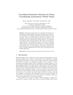
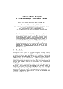
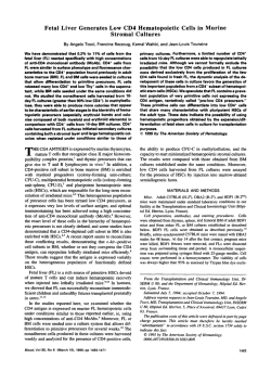
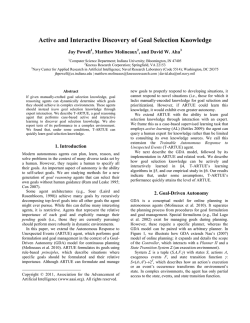
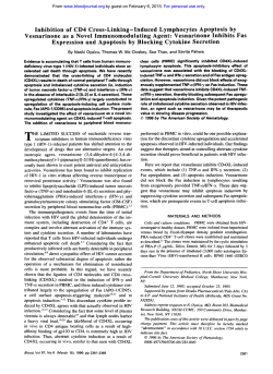
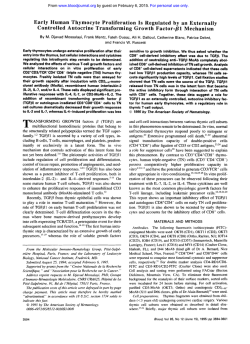
To appear in FLAIRS 2008
Learning Continuous Action Models
in a Real-Time Strategy Environment
Matthew Molineaux1, David W. Aha2, & Philip Moore1
1
Knexus Research Corporation; Springfield, VA 22153
Navy Center for Applied Research in Artificial Intelligence;
Naval Research Laboratory (Code 5514); Washington, DC 20375
[email protected]
2
Abstract
Although several researchers have integrated methods for reinforcement learning (RL) with case-based reasoning (CBR)
to model continuous action spaces, existing integrations typically employ discrete approximations of these models. This
limits the set of actions that can be modeled, and may lead to
non-optimal solutions. We introduce the Continuous Action
and State Space Learner (CASSL), an integrated RL/CBR
algorithm that uses continuous models directly. Our empirical study shows that CASSL significantly outperforms two
baseline approaches for selecting actions on a task from a
real-time strategy gaming environment.
1. Introduction
Real-time strategy (RTS) games are a popular recent focus
of attention for AI research (Buro 2003), and competitions
now exist for testing intelligent agents in these environments (e.g., AIIDE 2007; NIPS 2008). RTS environments
are usually partially observable, sequential, dynamic, continuous, and involve multiple agents (Russell and Norvig
2003). Typically, each player controls a team of units that
can gather resources, build structures, learn technologies,
and conduct simulated warfare, where the usual goal is to
destroy opponent units. Popular RTS environments for intelligent agent research include Wargus (Ponsen et al.
2005), ORTS (Buro 2002), and MadRTS, a game developed by Mad Doc Software, LLC.
A main attraction of RTS environments is that they can
be used to define and provide feedback for challenging
real-time control tasks (e.g., controlling single units, winning an entire game) characterized by large, continuous action and state spaces. However, the vast majority of intelligent agent research with RTS environments relies on discretizing these spaces (see §2.2). This process biases the
learner, and may render optimal actions inaccessible.
In this paper, we describe CASSL (Continuous Action
and State Space Learner), an algorithm that integrates
case-based reasoning (CBR) and reinforcement learning
(RL) methods that do not discretize these spaces. We
demonstrate and analyze CASSL’s utility in the context of
a task defined in MadRTS. Although previous research exists on continuous action and state spaces, as well as on
CBR/RL integrations, we believe ours is unique in how it
generates actions from stored experience.
Copyright © 2008, Association for the Advancement of Artificial Intelligence (www.aaai.org). All rights reserved.
Section 2 includes a brief introduction to the real-time
strategy environment we use along with a summary of related research. In Section 3, we introduce CASSL and explain how it extends our previous research. Section 4 describes an evaluation of its utility in comparison with simpler approaches. Finally, in Section 5 we provide greater
context for interpreting these results.
2. Background: Domain and Related Work
2.1 Real-Time Strategy Domain
In this paper, we focus on performance tasks whose space
of possible actions A and state space S are multi-dimensional and continuous. We use MadRTS, whose engine is
also used in the Empire Earth II™ game, for our evaluation. We also considered using Wargus, but chose to use
MadRTS because it is more reliable and supports scenarios
with higher military relevance.
We created MadRTS scenarios to test the capabilities of
intelligent agents for controlling a set of units using a feature-vector representation. Figure 1 shows a snapshot of
one of these scenarios, in which the units to be controlled
are the soldier units in the lower left corner. Their task is to
eliminate the opposing units in the scenario, which are located in the top left and lower right corners. An action in
this space corresponds to an order given by the agent to a
group of units. Each order directs the soldiers to travel
along a vector starting at their current position, attacking
any opponent units they encounter after completing this
movement. The lengths of these movements are variable,
so some actions have longer durations than others. We
evaluate an agent based on how many orders it gives, not
how much time it requires to complete a task.
The four dimensions of the continuous action space are:
– Heading  [0°,360°], where 0º is the heading from
the original midpoints of player and opponent soldiers
– Distance  [0,d], where d is the longest traversable
distance in the scenario
– Group size  [0,g], where g is the number of controllable units in the scenario
– Group selection  {all, strongest, leastRecent},
where the values indicate the method used to select a
group
The state space consists of eight features, which are defined relative to the midpoint of the player’s units:
Figure 1: The MadRTS State Space
–
–
–
–
–
Percentage of player’s initial soldiers still alive
Percentage of opponent’s initial soldiers still alive
Percentage of territories owned by the player
Heading to nearest opponent soldier  [0°,360°]
Heading to midpoint of opponent soldiers 
[0°,360°]
– Distance to midpoint of enemy soldiers  [0,d]
– Dispersal of opponent soldiers  [0,d], defined as the
median of distances from each opponent soldier to
the midpoint of all opponent soldiers
– Dispersal of player soldiers  [0,d]
At each time point, the agent receives a state vector with
the values of these features and selects an action to execute. For example, in Figure 1, the player units are at their
initial location in the lower left corner, and the opponents
are in the upper left and lower right corners. For both
sides, the percentage of original soldiers remaining is
100% and the percentage of territories (borders shown by
dotted lines) owned is 25%. The heading to the nearest opponent soldier is shown by Θoppnear. The heading to the
midpoint of opponent soldiers is Θmidopp and the distance
to their midpoint is shown as a line from midplayer to midopp.
The dispersal of opponent soldiers is labeled disp opp, while
the (small) dispersal of player soldiers is not shown.
2.2 Related Work
Several techniques for decision making have been tested in
RTS environments, including relational Markov decision
processes (Guestrin et al. 2003), integrated scheduling and
means-ends analysis planning (Chan et al. 2007), and simulation combined with Nash equilibrium approximation
(Sailer, Buro, and Lanctot 2007).
CBR and RL approaches have also been investigated
separately for RTS planning tasks. For example, CBR techniques have been designed to select action sequences (Aha,
Molineaux, and Ponsen 2005) and to construct plans from
behavioral cases extracted from and annotated by human
players (Otañón et al. 2007). RL techniques have been
used to select: action sequences (Ponsen et al. 2006),
choices defined in partial programs (Marthi et al. 2005),
and challenge-sensitive actions (Andrade et al. 2005). Un-
like these previous methods, CASSL does not discretize
the action space, and uses an integrated CBR/RL approach
to select primitive actions in an RTS task.
Previous approaches for learning in the context of continuous action spaces have been investigated separately for
CBR and RL methods. Among example CBR approaches,
Aha and Salzberg (1994) examined a set of supervised
learning approaches for a ball-catching task. Their algorithms restricted action selection to among those that had
been previously recorded, which limits the set of actions
that can be selected for a new state. Sheppard and Salzberg
(1997) describe a lazy Q-learning approach for action selection for a missile avoidance task in which the set of
states whose distance is within a threshold are located, and
among those the action is selected that has the highest Q
value. CASSL instead applies a quadratic model to the
nearest neighbors and selects an action corresponding to its
maximum. This differs from locally weighted regression
(Atkeson, Moore, and Schaal 1997), which computes a local linear model from a query’s neighboring cases.
Traditionally, RL methods have used eager learning
methods to help select actions from continuous action
spaces (Kaelbling, Littman, and Moore 1996, §6.2). For
example, these include training a neural network with
state-action input pairs and Q value outputs, and then applying gradient descent to locate actions with high Q values. Alternatively, this network could be used with an active learning process to test actions generated according to
a distribution whose mean and variance were varied so as
to find a local maximum. Gaskett et al. (1999) describe an
eager approach that performs interpolation with a neural
network’s outputs. They also survey continuous action Qlearning systems and note that most are eager and yield
piecewise-constant functions. In contrast, our approach
uses a lazy method for action selection and is not restricted
to piecewise-constant action-selection functions.
Takahashi et al. (1999) instead tessellate a continuous
action space in their Q-learning extension. CASSL does
not rely on decomposing the action space. Millán et al.
(2002) investigate a Q-learner that explores a continuous
action space by leveraging the Q-values of neighboring,
previously-explored actions. However, this limits action
selection to the set of previously explored actions. Buck et
al. (2002) heuristically select a set of actions that are distributed across the action space and select the one corresponding to the maximum-valued successor state. CASSL
instead selects actions used in neighbor states, dynamically
forms a quadratic model from them, and selects the action
that yields a maximum value according to this model.
Sharma et al. (2007) integrated CBR and RL techniques
in CARL, a hierarchical architecture that uses an instancebased state function approximator for its reinforcement
learner and RL to revise case utilities. They also investigated its application to scenarios defined using MadRTS.
However, CARL’s action space is discrete, whereas our
contribution is an integrated method for reasoning with
continuous action spaces. Santamaria et al. (1997) also examined integrated CBR/RL approaches that operate on
continuous action spaces and applied them to non-adversarial numeric control tasks. For example, this included a
CMAC (Albus 1975) approach for Q-learning that discretizes the set of possible actions and selects the action
with the highest Q-value. In contrast, CASSL dynamically
optimizes a continuous local model of the action-value
space, which allows access to all potential actions without
requiring a search over all of them.
Finally, unlike other Q-learning extensions that select
from among the actions in the (state) neighbors to a query,
Hedger (Smart & Kaelbling 2000) fits a quadratic surface
and selects an action that maximizes it. While CASSL also
calculates a regression surface, it is based on the value of
states that would occur if the state changed according to
trajectories observed in the past. Although these past trajectories may be inaccurate for the current state, the values
predicted are influenced less by nearby cases, and provide
a more diverse basis for the regression surface.
3. Continuous Action and Space Learning
We now describe CASSL (Continuous Action and Space
Learner), which integrates case-based and reinforcement
learning methods to act in an environment with continuous
states and actions. CASSL leverages our experiences with
CaT (Aha et al. 2005), which uses CBR techniques (but not
RL) to control groups in Wargus (Ponsen et al. 2005), a dynamic, non-episodic, and nearly deterministic RTS environment. CaT’s control decisions focus on tactic selection,
where tactics are comparatively long sequences of primitive actions lasting a significant fraction of a trial.
3.1 Motivation for this Integrated Approach
CaT has two limitations that CASSL addresses. First, CaT
was designed for an abstract action space (i.e., it selects
from among a small set of pre-defined tactics) and required
a large state-space taxonomy; it was not designed for a
knowledge-poor continuous action domain or, more generally, domains that have a large number of primitive actions.
Techniques that make decisions of smaller granularity may
permit greater control, and eliminate the need for creating
tactics in advance. Greater control may also increase task
performance and reduce dependence on an external source
of tactics. For example, suppose CaT’s opponent tries to
gain an advantage via early use of air units. If none of
CaT’s tactics can create air units early on, it will probably
lose often. With direct access to primitive actions that create new units, CASSL is not prone to this problem.
Second, CaT cannot reason about causal relations
among states, which can be used to improve credit assignment. Standard RL techniques for representing value functions and action-value functions can represent these relations (Sutton and Barto 1998), which motivates our investigation of an integrated CBR/RL approach in this paper. For
example, if CaT tends to pick a poor-performing tactic subsequent to a good tactic, then it would average the performance across all successor tactics. In contrast, CASSL instead uses a sample backup procedure that can more quickly improve the accuracy of performance approximations.
3.2 CASSL Algorithm
CASSL is a case-based reasoner that responds to each time
step of a game trial by executing a function LearnAct,
T: Transition case base <S × A × ΔS>
V: Value case base <S ×  >
---------------------------LearnAct(s i-1 , a i-1 , s i, r i-1 ) =
T ← retainT(T, s i-1 ,a i-1 , s i-s i-1 )
V←
retainReviseV(V, s i-1 ,retrieve(V,s i ))
C ← retrieve(T, s i)
M← 
cC: M ←
M  <c.a, retrieve(V,s i + c.Δs)>
a i ← arg max aA reuse(M, a)
return a i
; Update transition case base
; Update value case base
; Retrieve sim ilar transition cases
; Initialize the m ap of actions to values
; Populate it for retrieved cases’ actions
; Fetch action w/ m ax predicted rew ard
using the Nelder-M ead sim plex method
Figure 2: CASSL’s learning and action selection function
which updates CASSL’s case bases and returns a new action to be performed. LearnAct inputs a prior state si-1S,
an action ai-1A which was taken in state si-1, the state siS
which resulted from applying ai-1 in si-1, and a reward r.
It outputs a recommended action aiA. States in S and actions in A are represented as real-valued feature vectors.
Figure 2 details CASSL’s LearnAct function. It references two case bases, which are updated and queried during an episode. The first is the transition case base T:
S×A×ΔS, which models the effects of applying actions. T
contains observed state transitions that CASSL uses to help
predict future state transitions. These have the form:
cT = <s, a, Δs>
The second case base is the value case base V: S×,
which models the value of a state. It contains estimates of
the sum of rewards that would be achieved by CASSL
starting in a state s and continuing to the end of a trial using its current policy. Value cases have the form:
cV = <s, v>
Each of CASSL’s two case bases supports a case-based
problem solving process consisting of a cycle of case retrieval, reuse, revision, and retention (Aamodt and Plaza
1994). These cycles are closely integrated because a solution to a problem in T forms a problem in V; CASSL solves
these problems in tandem to select an action.
At the start of a trial each of CASSL’s case bases is initialized to the empty set. CASSL retains new cases and revises them through its application to a sequence of gameplaying episodes. For each new state si that arises during an
episode, LearnAct is called with its four arguments.
LearnAct begins with a case retention step in T; if an experience occurs that is not correctly predicted by T, a new
case cT,i = <si-1, ai-1, Δs> is added, where Δs = si-si-1 (a vector
from the prior to the current state). Retention is controlled
by two parameters τT , and σT (not shown in Figure 2); cT,i is
retained if either the distance dT(cT,i,1NN(V,cT,i)) between
cT,i and its nearest neighbor in T is less than τT, or if the distance dT(cT,i.Δs, T(si-1, ai-1)) between the actual and the estimated transitions is greater than the maximum error per-
1
a1
a3
si
SY
si a1 si+1
SY
a2 a3
a2
0
2.Get their predicted
next states (si+1)
a2
a3
3.Get predicted values
of these next states
a2
V
a3
a1
0
A
ai
1
V
a1
Sx
1.Retrieve actions
(a1,…,ak) of k-NN
a2
V
si+1
si+1
Sx
1
0
A
4.Compute a value
model from them
a3
a1
A
5.Select action ai with
max predicted value
Figure 3: CASSL’s algorithm for action recommendation, where Sx and SY are hypothetical state features
mitted, σT. Transition cases are never revised, under the assumption of a deterministic environment.
The second line in LearnAct performs conditional case
retention and revision for V. A new case cV,i is added to V
only if the state distance dV(cV,i,1NN(V,cV,i)) to its nearest
neighbor in V is greater than τV (not shown in Figure 2).
New cases are initialized using the discounted return (Sutton and Barto 1998):

k
V ,i
i 1
k 1
k i
Otherwise, cV,i’s k-nearest neighbors are revised to better
approximate the actual value of this region of the state
space. The state value vk associated with each nearest
neighbor cV,kkNN(V,cV) is revised according to its contribution to the error in estimating the value of vi-1:
c
s ,  γ r
vk vk  α  ri 1  γvi  vk  
as described for the step that updates V.
CASSL then creates a multi-dimensional model of this
action-value map using quadratic regression (step 4 in Figure 3), which is necessary due to the continuous nature of
the state and action spaces. We chose quadratic regression
because a quadratic function often produces a useful peak
that is not at a point in the basis mapping, thereby encouraging exploration. Higher orders of regression may also
produce such results, but are more computationally expensive, and we would like to produce a result in real time.
The final step locates the action that maximizes this
model, and adds it to M. To compute this, we use Flanagan’s (2007) implementation of the Nelder-Mead simplex
method, a well-known method for finding a maximum value of a general n-dimensional function.
The quadratic estimate of the value of the discovered action is less accurate than a case-based prediction. Thus, we

K  d cV ,i , cV ,k 
 K d c
V ,i
cV , j kNN (V ,cV )
where vk is the value associated with neighbor cV,k, α (0 ≤ α
≤ 1) is the learning rate, γ (0 ≤ γ ≤ 1) is a geometric discount factor, and the Gaussian kernel function K(d) = exp(d2) determines the relative contributions of the k-nearest
neighbors.
Figure 3 summarizes the remaining (action-recommendation) steps of LearnAct, which next retrieves C, the set
of transition cases in T whose states are similar to si. This
identifies states that are reachable from the current state,
and actions for transitioning to them (see step 1 in Figure
3). CASSL uses a simple k-nearest neighbor algorithm on
states for case retrieval. However, we set k to be large so as
to retrieve enough information for the later regression step
to succeed. Specifically:
2
a
 a 1,
2
where |a| is the size of an action vector.
Next, for each nearest neighbor cT,k = <sk,ak,Δsk>,
CASSL computes the predicted next state that results from
applying ak in state si, thus creating a mapping M from actions to the value of the expected resulting state. This value
is calculated by performing the vector addition Δsk + si,
which yields the predicted state si+1. Then V is reused to
calculate the expected value of state si+1 (step 3 in Figure
3). Retrieval and reuse are performed in the same fashion
k
, cV , j 
iteratively re-create the model, incorporating more accurate predictions, by repeating Steps 4 and 5 (Figure 3) until
a similar action is found on two successive iterations, or
until 50 iterations have passed. Similarity between successive actions is defined as a Euclidean distance less than a
small threshold value; we use 0.0001 as the threshold.
4. Evaluation
Our empirical study focuses on analyzing whether CASSL’s continuous action model significantly outperforms a
similar algorithm that instead employs a discrete action
model on a task defined in MadRTS. As an experimentation platform, we used TIELT (2007), the Testbed for Integrating and Evaluating Learning. TIELT is a free tool that
can be used to evaluate the performance of an agent on
tasks in an integrated simulation environment. TIELT managed communication between MadRTS and the agents we
tested, ran the experiment protocol, and collected results.
We assessed performance in terms of a variant of regret
(Kaelbling et al. 1996) that calculates the difference between the performances of two algorithms over time as a
percentage of optimal performance. The domain metric
measured is the number of steps required to complete the
task. As described in Section 2.1, each step corresponds to
an order given to a group of units. After 200 steps, a trial is
cut off, so a value of 200 corresponds to failure.
We compared the performance of CASSL versus two
baseline algorithms. The first is random, which at each
time step selects an action randomly from a uniform distribution over the 4-dimensional action space.
The second algorithm is a CMAC controller (Albus
1975), a commonly used algorithm for performing RL
tasks in continuous state spaces. It uses a set of overlapping tilings of the state-action space to approximate the RL
Q(s,a) function. It executes a query by averaging the value
of the tile in each tiling that corresponds to the state-action
input. For this experiment, we used five tilings, evenly offset from one another. There are 4 tiles per dimension and
12 dimensions in S×A, which yields a tiling size of 412 and
a total of 5412 = 83.9M tiles. The structure and basic operations of our CMAC are similar to those described in (Santamaria et al., 1998) with λ=0.9.
For both RL algorithms (CASSL and CMAC), we set
Figure 4: Learning performance
α=0.2, γ=1.0, and ε=0.5 (exploration parameter). Both α
and ε were decreased asymptotically to 0 over time. For
CASSL, we also set λ=0, k=21, τT=0.8, τV=0.05, and
σT=0.2. We briefly conducted a manual parameter tuning
process to obtain reasonable performances from both algorithms, but did not attempt to optimize their settings.
The MadRTS scenario used for this evaluation has a size
of 100 x 100 tiles, each covered with flat terrain. In the
starting position, 3 “U.S. Rifleman” (powerful) units controlled by player 1 are clustered around tile <20,22>, 3 “Insurgent5_AK47” (less powerful) units controlled by player
2 are clustered about <2,98>, and 1 “Insurgent1_AK47”
(powerful) unit controlled by player 2 is at <98,2>. The
victory condition is set to a value of “conquest”, and diplomacy between players 1 and 2 is set to “hostile”. At these
settings, the opponent will attempt to hold his ground and
destroy all hostile units that enter visual range. All other
settings have their default values.
We ran each agent for 10 replications, each on 1000
training trials, and tested on 5 trials after every 25 training
trials. We report the average testing results. Although each
agent learned on-line within a testing trial, its memory was
recorded beforehand and reset after each test. To ensure
Figure 5: Early learning performance
that trials ended in a reasonable amount of time, we cutoff
any that did not complete after 200 time steps; no reward
was assigned for the final action of a cutoff trial. A reward
of −1 was given at each step unless the agent accomplished
its goal (reward=1000) by eradicating the opponent’s units.
Figure 4 displays the results. The curves shown here are
monotonically non-increasing because we report the minimum steps taken (per algorithm) on any trial so far in a
replication and average over these curves. This measurement is reasonable because prior testing performances can
be repeated by restoring the state of the learner; it is more
forgiving to algorithms that do not guarantee that learning
will never decrease performance.
The regret of CMAC compared to CASSL is 3.53, which
is statistically significant (p=0.001). Thus, CASSL, using
its best learned behavior so far, is 3.53% closer to optimal
performance. Comparing CASSL to the random agent, the
regret is 38.66, which is again significant (p < 0.001).
Figure 5 compares the early learning performance of
CMAC and CASSL up to 200 trials. This period is particularly interesting because it shows that CASSL learns to do
well earlier than CMAC. The regret during this period (0200 training trials) is 9.74 with p=0.017.
5. Discussion
Our goal was to demonstrate that selecting from among all
possible continuous actions rather than a priori reducing
their set (e.g., via discretization) can significantly improve
performance. However, we assessed this on only a single
scenario, and versus only two other algorithms. In future
work, we will compare CASSL’s performance, empirically
and via a computational complexity analysis, with other algorithms that can process continuous action spaces over a
range of learning and performance tasks. This will include
variants of CASSL that discretize the action space.
Other models for regression of the local action-value
function (e.g., some higher-order polynomial or other function entirely) might outperform the model we used. Also, a
model-free variant of CASSL in which the action-value
function is represented directly should be studied. The two
case bases should scale up to higher dimensions more easi-
ly, but we have not empirically verified this.
We have not optimized CASSL’s performance (e.g., employing more selective methods for using neighbors to create action recommendations). This remains future work.
RTS domains often involve a variety of similar tasks
with different initial conditions and varied goals. For example, a larger group of units might need to be destroyed
at a variety of locations both near and far from the agent’s
home base. We plan to analyze the capability of CASSL
and other RL agents to generalize over different goals and
starting conditions in an RTS domain.
6. Conclusions
We introduced a methodology that, unlike our earlier approach (Aha et al. 2005), can learn and reason with continuous action spaces. To do this it integrates case-based reasoning and reinforcement learning methods, and its implementation in CASSL significantly outperformed two baseline approaches on a real-time strategy gaming task.
The primary contribution of this paper was a lazy learning approach for action generation in a continuous space.
In our future work, we will compare this approach with
variants of CASSL that are eager, that adopt a Q-learning
framework, and/or discretize the action space.
Acknowledgements
Thanks to DARPA (#07-V176) for supporting this work
and to the reviewers for their helpful comments.
References
Aha, D.W., Molineaux, M., & Ponsen, M. (2005). Learning to
win: Case-based plan selection in a real-time strategy game.
Proceedings of the Sixth International Conference on CaseBased Reasoning (pp. 5-20). Chicago, IL: Springer.
Aha, D.W., Muñoz-Avila, H., & van Lent, M. (Eds.) (2005).
Reasoning, Representation, and Learning in Computer
Games: Papers from the IJCAI Workshop (Technical Report
AIC-05-127). Washington, DC: Naval Research Laboratory,
Navy Center for Applied Research in Artificial Intelligence.
Aha, D. W., & Salzberg, S. L. (1994). Learning to catch: Applying nearest neighbor algorithms to dynamic control tasks. In P.
Cheeseman & R. W. Oldford (Eds.), Selecting Models from
Data: AI and Statistics IV. New York: Springer.
AIIDE (2007). 2007 ORTS RTS Game AI Competition.
[http://www.cs.ualberta.ca/~mburo/orts/AIIDE07]
Albus, J.S. (1975). A new approach to manipulator control: The
cerebellar model articulation controller. Journal of Dynamic
Systems, Measurement, and Control, 97(3), 220-227.
Andrade, G., Ramalho, G., Santana, H., & Corruble, V. (2005).
Extending reinforcement learning to provide dynamic game
balancing. In (Aha et al., 2005).
Atkeson, C., Moore, A., & Schaal, S. (1997). Locally weighted
learning. Artificial Intelligence Review, 11(1-5), 11-73
Buck, S., Beetz, M., & Schmitt, T. (2002). Approximating the
value function for continuous space reinforcement learning in
robot control. Proceedings of the International Conference on
Intelligent Robots and Systems (pp. 1062-1067). Lausanne,
Switzerland: IEEE Press.
Buro, M. (2002). ORTS: A hack-free RTS game environment.
Proceedings of the International Computers and Games Conference (pp. 280-291). Edmonton, Canada: Springer.
Buro, M. (2003). Real-time strategy games: A new AI research
challenge. Proceedings of the Eighteenth IJCAI (pp. 15341535). Acapulco, Mexico: Morgan Kaufmann.
Chan, H., Fern, A., Ray, S., Wilson, N., & Ventura, C. (2007).
Online planning for resource production in real-time strategy
games. In Proc. of the In. Conference on Automated Planning
and Scheduling. Providence, Rhode Island: AAAI Press.
Gaskett, C., Wettergreen, D., & Zelinski, A. (1999). Q-learning in
continuous state and action spaces. Proceedings of the Twelfth
Australian Joint Conference on Artificial Intelligence (pp. 417428). Sydney, Australia: Springer.
Guestrin, C., Koller, D., Gearhart, C., & Kanodia, N. (2003).
Generalizing plans to new environments in relational MDPs.
Proceedings of the Eighteenth IJCAI (pp. 1003-1010). Acapulco, Mexico: Morgan Kaufmann.
Kaelbling, L.P., Littman, M.L., & Moore, A.W. (1996). Reinforcement learning: A survey. JAIR, 4, 237-285.
Marthi, B., Latham, D., Russell, S., & Guestrin, C. (2005). Concurrent hierarchical reinforcement learning. Proceedings of the
Nineteenth International Joint Conference on AI. (pp. 779785). Edinburgh, Scotland: Professional Book Center.
del R. Millán, J., Posenato, D., & Dedieu, E. (2002). Continuousaction Q-learning. Machine Learning, 49,247–265.
Flanagan, M. (2007). Michael Thomas Flanagan’s Java Scientific
Library. [http://www.ee.ucl.ac.uk/~mflanaga]
NIPS (2008). RL 2008 Competition: Real-Time Strategy.
[http://rl-competition.org/content/view/20/36]
Ontañón, S., Mishra, K., Sugandh, N., & Ram, A. (2007). Casebased planning and execution for real-time strategy games.
Proceedings of the Seventh International Conference on CaseBased Reasoning (pp. 164-178). Belfast, N. Ireland: Springer.
Ponsen, M.J.V., Lee-Urban, S., Muñoz-Avila, H., Aha, D.W., &
Molineaux, M. (2005). Stratagus: An open-source game engine for research in RTS games. In (Aha et al., 2005).
Ponsen, M.S.V., Spronck, P., Muñoz-Avila, H., & Aha, D.W.
(2006). Automatically generating game tactics through evolutionary learning. AI Magazine, 27(3), 75-84.
Ram, A., & Santamaria, J.C. (1997). Continuous case-based reasoning. Artificial Intelligence, 90(1-2), 25-77.
Russell, S., & Norvig, P. (2003). Artificial intelligence: A modern
approach (2nd ed.). Upper Saddle River, NJ: Prentice Hall.
Sailer, F., Buro, M., Lanctot, M. (2007). Adversarial planning
through strategy simulation. In Proceedings of the Symposium
on Computational Intelligence in Games. Hawaii, HO: IEEE.
Santamaria, J.C., Sutton, R., & Ram, A. (1998). Experiments with
reinforcement learning in problems with continuous state and
action spaces. Adaptive Behavior, 6(2):163-217.
Sharma, M., Holmes, M., Santamaria, J.C., Irani, A., Isbell, C., &
Ram, A. (2007). Transfer learning in real-time strategy games
using hybrid CBR/RL. In Proceedings of the Twentieth International Joint Conference on Artificial Intelligence.
[http://www.ijcai.org/papers07/contents.php]
Sheppard, J.W., & Salzberg, S.L. (1997). A teaching strategy for memory-based control. AI Review, 11(1-5), 343-370.
Smart, W.D., & Kaelbling, L.P. (2000). Practical reinforcement
learning in continuous spaces. Proceedings of the Eighteenth
ICML (pp. 903-910). Stanford, CA: Morgan Kaufmann.
Sutton, R., & Barto, A. (1998). Reinforcement learning: An introduction. Cambridge, MA: MIT Press.
Takahashi, Y, Takeda, M., & Asada, M. (1999). Continuous valued Q-learning for vision-guided behavior acquisition. Proceedings of the Int. Conf. on Multisensor Fusion and Integration for Int. Sys. (pp.255-260). Taipei, Taiwan: IEEE Press.
TIELT (2007). Testbed for integrating and evaluating learning
techniques. [http://www.tielt.org]