46th Lunar and Planetary Science Conference (2015) 1797.pdf AUTOMATIC CRATER DETECTION IN LARGE SCALE ON LUNAR MARIA. M. Machado, L. Bandeira and P. Pina, CERENA/IST/UL, Lisbon, Portugal, {marlene.machado, lpcbandeira, ppina}@tecnico.ulisboa.pt. Introduction: In a little more than one decade, crater detection algorithms (CDA) have greatly evolved in their conception and in the methodological ingredients used, from the more classic image analysis and pattern recognition operators [1, 2, 3, 4] to the more up-to-date and adaptive tools [5, 6, 7, 8, 9], providing more robust processing sequences able to successfully deal with the large variety of cratered landscapes all over the Solar System. These have naturally been mainly developed and tested for those surfaces where imagery is more abundant, Mars and the Moon. More recently, CDA are also being applied on Mercury [10, 11], Phobos [12] and Vesta [10]. In this way, the robustness of the CDA has been proved undoubtedly in a wider type of surfaces, also contributing to update crater catalogues on Mars [13], Moon [14] and Phobos [12]. But even in these studies the figures involved, when optical images are concerned, are around some few thousands of craters. Our main objective in this work is to demonstrate that the detection of a huge amount of craters (hundreds of thousands) with an automated approach in relatively large regions covered by the assemblage of several adjacent images (mosaics), captured in distinct time periods, can be trusted. Dataset and Methodology: In this abstract we focus our study on the Moon, in particular in Sinus Iridum region (44.1° N, 31.5° W), a mare filled crater of about 236 km in diameter, through the analysis of a Kaguya (SELENE) [15] Terrain Camera (TC) Evening illumination tile set with spatial resolution of 7.4 m/pixel, released by the SELENE team [16] and rereleased by Astrogeology/USGS [17] to detect craters with a dimensional range of diameters between 100 and 1500 meters. Instead of processing the entire region at once, we analyzed smaller areas at each time, with dimension (2048 x 2048 pixels with a 200 pixels overlap between adjacent tiles) that permitted an efficient computational performance and the detection of the entire impact structure within the same tile. A total of 480 tiles in the mare region were generated this way, being 12 of them selected to train and test our approach: 6 of the tiles were concentrated around the same area, located in the southern part of the mare, while the other 6 tiles were selected from dispersed locations of Sinus Iridum to contain the diversity of the mare surface (Figure 1), where we have manually cataloged almost 190,000 craters. 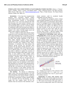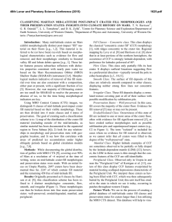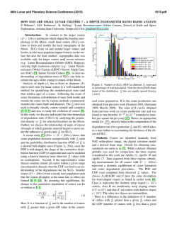Figure 1 - Sinus Iridum mare on a mosaic built from images captured by the Terrain Camera from Kaguya. The numbered squares indicate the sample tiles used. [image credits: USGS , Kaguya]. Our Crater Detection Algorithm (CDA) searches for suitable crater candidates defined as pairs of shaded/highlighted crescent regions and for which a set of textural image features (Haar-like) are extracted, and used, together with non-crater examples, for training a SVM-Support Vector Machines classifier, previously described in [8, 18]. Results: Using the tiles as training and testing units, we selected each individual tile for training and applied the detection algorithm to all the remaining tiles for testing in a cross-validation strategy. To evaluate the performance of our CDA we measured the detection percentage D = 100 x TP/(TP + FN), the quality percentage Q = 100 x TP/(TP + FP + FN) and the branching factor B = FP/TP. Here, TP stands for the number of true positive detections (detected craters that are actual craters), FP stands for the number of false positive detections (detected craters that are not), and FN stands for the number of false negative “detections” (non-detection of real craters). D can be treated as a measure of crater-detection performance, Q as an overall measure of algorithm performance, and B as a measure of delineation performance. These results are summarized in Table 1 and illustrated by Figure 2 46th Lunar and Planetary Science Conference (2015) where it can be seen the application of our CDA to tile 439 of the test scene. Table 1: Performance of our CDA Test site D (%) 85.12 Q (%) 75.22 FDR (%) 13.39 B 0.15 Conclusions: The performances achieved are considered very good (85% for correct detections and 13% for false positive detections) for a ground-truth dataset comprising about 190,000 craters located in several locations of Sinus Iridum mare. 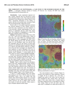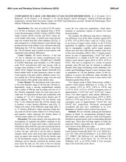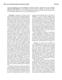Figure 2 - Evaluation of automated crater detection in tile 439. The colors of the circles have the following meaning: green – true detections (true positives); red – incorrect detections (false positives); blue – missing detections (false negatives). 1797.pdf The quality rate decreased 3% from the previous study of this region [18] but the dataset is 52x larger. Furthermore, the individual results for each tile show that there is a dependence on the choice of tile selected for training (variation of about 10% of the overall rates), with a direct relation with the number of craters within each tile. When selecting a region for training one must be careful not only to choose an area with enough examples but examples with all the geomorphological variety present in the test site. The extension of the optimal experimental setup to the entire mare permitted to identify about 600,000 circular structures, whose visual inspection indicates a very similar pattern to the tiles where quantitative performances were obtained. Acknowledgements: We would like to thank Astrogeology/USGS, and in particular Trent Hare, for providing the data used here; MM and LB (SFRH/BPD/79546/2011) acknowledges support by FCT (Portugal). References: [1] Leroy B. et al. (2001) Image and Vision Computing, 19:787-792. [2] Michael G. (2003) PSS, 51:563-568. [3] Barata T. (2004) LNCS, 3212:489-496. [4] Bandeira L. et al. (2007) IEEE TGRS, 45(12):4008-4015. [5] Martins et al. (2009) IEEE GRSL, 6(1):127-131. [6] Urbach E.R. and Stepinski T.F. (2009) PSS, 57:880–887. [7] Burl M.C. and Wetzler P.G. (2011) Machine Learning, 84:341367. [8] Bandeira L. et al. (2012) ASR, 49(1):64-74. [9] Jin S. and Zhang T. (2014) PSS, 99:112-117. [10] Salamuniccar G. (2014) LPSC XLV, Abstract #1785. [11] Pedrosa M. (2014) this volume. [12] Salamunićcar G. et al. (2014) ASR, 53:1798-1809. [13] Salamunićcar G. et al. (2012) PSS, 60:236-247. [14] Salamunićcar G. et al. (2014) ASR, 53:1783-1797. [15] Haruyama J. et al. and the LISM Working Group (2008) Earth Planets Space, 60:243-255. [16] Kato M. et al., Selene Project Team (2006) LPSC XXXVII, Abstract #1233. [17] Isbell C. et al. (2014) LPSC XLV, Abstract #2268. [18] Bandeira L. et al. (2014) LPSC XLV, Abstract #2240.