1. Art and Diseño

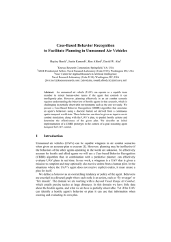
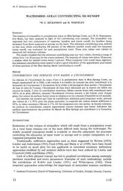
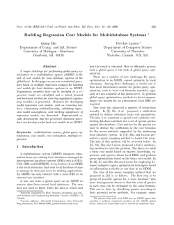
Supplement of Hydrol. Earth Syst. Sci. Discuss., 12, 1205–1245, 2015
http://www.hydrol-earth-syst-sci-discuss.net/12/1205/2015/
doi:10.5194/hessd-12-1205-2015-supplement
© Author(s) 2015. CC Attribution 3.0 License.
Supplement of
High-quality observation of surface imperviousness for urban runoff
modelling using UAV imagery
P. Tokarczyk et al.
Correspondence to: P. Tokarczyk ([email protected])
S1
Remote sensing methods to extract the imperviousness maps
A considerable amount of remote sensing research has been devoted to the problem of mapping
impervious surfaces. Here, we review some of the previous studies and evaluate them in respect of
710
the datasets and classification methods. Furthermore, we focus on the studies which use the classified
land-use to predict urban rainfall runoff.
Whereas few studies have used low-resolution (GSD > 100m) satellite sensors, such as MODIS
(Lu et al., 2008; Boegh et al., 2009), AVHRR (Carlson and Arthur, 2000) and DMSP-OLS (Elvidge
et al., 2007; Lu et al., 2008), the large part of the research in this area focused on medium and high
715
spatial resolution satellite data. Because of its exceptional temporal resolution, Landsat is still the
most popular satellite platform. A large number of authors used Landsat 5 TM (Civco et al., 2002;
Carlson, 2004; Bauer et al., 2008; Yuan and Bauer, 2006; Li et al., 2011; Parece and Campbell, 2013;
Dougherty et al., 2004) and Landsat 7 ETM+ data (Civco et al., 2002; Yang et al., 2003; Wu and
Murray, 2003; Lu and Weng, 2006; Lee and Lathrop, 2006; Powell et al., 2007; Chormanski et al.,
720
2008; Chabaeva et al., 2009; Van de Voorde et al., 2009) for analysing impervious surface cover.
Other examples of using images acquired by high resolution platforms include SPOT (Yang et al.,
2009; Li et al., 2011; Tan et al., 2009) and ASTER (Weng and Hu, 2008; Hu and Weng, 2009; Weng
et al., 2009).
However, recent developments of remote sensing imaging sensors and platforms gave access to
725
VHR imagery. Examples of VHR satellite sensors application to impervious surfaces mapping include Ikonos (Cablk and Minor, 2003; Lu and Weng, 2009; Mohapatra et al., 2008; Chormanski
et al., 2008; Van de Voorde et al., 2009; Mathieu et al., 2007), and QuickBird (Lu et al., 2008; Yuan
and Bauer, 2006; Zhou and Wang, 2008). Except of satellite imagery, aerial images are also an important source of information. Many studies used aerial orthophotos only as a reference check to
730
satellite imagery (Yang et al., 2003; DeBusk et al., 2010; Parece and Campbell, 2013). However
few attempts to automatically map imperviousness using such data were made (Nielsen et al., 2011;
Dougherty et al., 2004; Hodgson et al., 2003; Zhou and Wang, 2008; Fankhauser, 1999; Lee and
Heaney, 2003).
One possible way to extract imperviousness from images is to interpret them manually. Even
735
though this is the most reliable method, and has been used in few studies (e.g. Lee and Heaney
(2003)), it is very costly in terms of time and money. Therefore it is common to automate the process by using image classification. Maybe the simplest method is to assume that only vegetation
is pervious and rely on the normalized differential vegetation index (NDVI) (Nielsen et al., 2011;
Carlson and Arthur, 2000). Many of the studies use more advanced classification methods, such as
740
object based image analysis (OBIA) (Zhou and Wang, 2008; Hodgson et al., 2003; Nielsen et al.,
2011; Mathieu et al., 2007). Other examples include maximum likelihood classifier (Fankhauser,
1
1999; Hodgson et al., 2003), spectral mixture analysis (SMA) (Small, 2003; Van de Voorde et al.,
2009; Weng et al., 2009), artificial neural networks (ANN) (Chormanski et al., 2008; Van de Voorde et al., 2009; Lee and Lathrop, 2006), classification and regression trees (CART) (Yang et al.,
745
2003; Li et al., 2011; Dougherty et al., 2004) and rule-based classifiers (Hodgson et al., 2003). Some
of the mentioned methods also use the perviousness maps for urban drainage modelling like we
do (Nielsen et al., 2011; Melesse and Wang, 2008; Chormanski et al., 2008; Dougherty et al., 2004;
Lee and Heaney, 2003; Fankhauser, 1999). However, to our best knowledge no studies exist, that
used UAV-based imagery to extract imperviousness information, and to use it in the field of urban
750
drainage modelling.
S2 UAV platform
The UAV platform used in this study is an autonomous fixed-wing drone produced by senseFly SA
(cf. http://www.senseFly.com). Table S1 includes detailed information about the platform.
Weight (incl. camera)
ca. 0.69 kg
Wingspan
96 cm
Material
EPP foam, carbon structure and composite parts
Propulsion
Electric pusher propeller, 160 W brushless DC motor
Battery
11.1 V, 2150 mAh
Camera (supplied)
16 MP IXUS/ELPH
Cameras (oprional)
S110 RGB, thermoMAP
Max. flight time
50 min
Nominal speed
40-90 km/h
Wind resistance
Up to 45 km/h (12 m/s)
Radio link range
Up to 3 km
Max. coverage (single flight)
Up to 12 km2
Cost
ca. 20’000 CHF (Drone + Software)
Table S1. Specifications of the UAV used in the study (source: http://www.senseFly.com)
755
The imaging unit mounted on a UAV was a customized version of Canon IXUS 127 HS compact
camera. Table S2 includes its specifications.
2
Camera effective pixels
ca. 16.1 million
Lens’ focal length
4.3 - 21.5 mm (35 mm equivalent: 24 - 120 mm)
Interfaces
Hi-speed USB, HDMI Output, Analog audio
output, Analog video output (NTSC/PAL)
Dimensions
93.2 × 57.0 × 20.0 mm
Weight
ca. 135 g (incl. battery and memory card)
Table S2. Specifications of the Canon IXUS 127 HS Camera
S3
Exploratory data analysis of the importance of image source and processing method for
the surface runoff
760
S3.1
Regression
Imperviousness
Please refer to Table S3and Figure S3.
Here we try to answer a following question: Which has the greater influence/is stronger correlate
765
with a change in imperviousness and surface runoff characteristics, the image source or the processing method?
Model and results
Here we present logit-transformation of imperviousness. This was done to constrain the model out-
770
put to the range between 0 and 1 and not to improve the statistical assumptions regarding the errors
of the data generating process.
Description/Interpretation
UAV images seem to be negatively correlated with the imperviousness. The effect is not really strong.
775
Regarding the methods, there seems to be no influence, because the estimated linear relation is practically negligible. In addition, there is no evidence for interactions between the image source and the
processing method.
3
Peak runoff
780
Model and results
Please refer to Table S4 and Figure S4
Description/Interpretation
785
UAVdata generally seem to produce slightly smaller peaks, whereas the RQE method is positively
correlated to peak hight. However both effects are not significant by any means. There are no interactions of these two. Statistical assumptions are not fulfilled.
790
Runoff volume
Model and results
Please refer to Table S5 and Figure S5
795
Description/Interpretation
UAV data generally seem to produce slightly runoff volumes, whereas the RQE method is positively
correlated to runoff volume. However both effects are not significant by any means. There are no
interactions of these two. Statistical assumptions are not fulfilled.
800
Time to peak
Analysis was not performed, because exploratory analysis suggest that the differences between the
different image sources are negligibly small.
805
S4 Pipe flow predictions
Please refer to Figure S6
4
Figure S1. Scatterplot of surface runoff characterstics for the 307 individual subcatchments of the Wartegg
SWMM model. Black = Ortho fotos, Red= UAV images. A_eff: effective area, Imp: imperviousness
5
Figure S2. Scatterplot of surface runoff characterstics for the 307 individual subcatchments of the Wartegg
SWMM model. Green= ML, Blue = RQE. A_eff: effective area, Imp: imperviousness
6
Table S3. Summary results of the regression analysis. The negative sign of the estimated slope parameter suggests
that the UAV images generally go together with a lower imperviousness. In addition, the influence of the image
source seems to be larger than that of the classification method, although the high p-values for all parameters
suggest that it is not very likely that the observed values of imperviousness were to have occurred under the
given statistical model.
Dependent variable:
Volume
−301.699
DataUAV
(331.033)
MethodRQE
298.671
(331.033)
DataUAV:MethodRQE
199.362
(468.151)
3,893.406∗∗∗
Constant
(234.075)
Observations
R
1,228
2
0.003
Adjusted R2
0.001
Residual Std. Error
4,101.333 (df = 1224)
F Statistic
Note:
1.274 (df = 3; 1224)
∗
p<0.1; ∗∗ p<0.05; ∗∗∗ p<0.01
7
Figure S3. Diagnostic plots of the regression analysis. It is obvious that the statistical assumptions are not
fulfilled very well and that the observe imperviousness is not well explained.
8
Table S4. Summary results of the regression analysis for peak runoff. The negative sign of the estimated slope
parameter suggests that the UAV images generally go together with a lower stormwater peak flow. Here, the
influence of the image source seems to be in the same order of magnitude than that of the classification method,
although the former is negatively correlated and the latter has a positive correlation with peak runoff. Again,
the high p-values for all parameters suggest that it is not very likely that the observed peak runoff values were
to have occurred under the given statistical model.
Dependent variable:
Peak
−0.065
DataUAV
(0.067)
MethodRQE
0.068
(0.067)
DataUAV:MethodRQE
0.038
(0.094)
0.826∗∗∗
Constant
(0.047)
Observations
1,228
R2
0.004
Adjusted R2
0.001
Residual Std. Error
0.827 (df = 1224)
F Statistic
Note:
1.507 (df = 3; 1224)
∗
p<0.1; ∗∗ p<0.05; ∗∗∗ p<0.01
9
Figure S4. Diagnostic plots of the regression analysis. It is obvious that the statistical assumptions are not
fulfilled very well and that the observe imperviousness is not well explained.
10
Table S5. Summary results of the regression analysis for runoff volume.
Dependent variable:
Volume
−301.699
DataUAV
(331.033)
MethodRQE
298.671
(331.033)
DataUAV:MethodRQE
199.362
(468.151)
3,893.406∗∗∗
Constant
(234.075)
Observations
R
1,228
2
Adjusted R
0.003
2
0.001
Residual Std. Error
4,101.333 (df = 1224)
F Statistic
Note:
1.274 (df = 3; 1224)
∗
p<0.1; ∗∗ p<0.05; ∗∗∗ p<0.01
11
Figure S5. Diagnostic plots of the regression analysis. It is obvious that the statistical assumptions are not
fulfilled very well and that the observe imperviousness is not well explained.
12
Figure S6. Distribution of calibration parameter (Decay K: infiltration decay rate after HORTON; MaxRate:
maximum infiltration rate after HORTON; width: conceptual parameter describing the width of a subcatchment; Add.area: conceptual parameter describing event-based sewer infiltration) values identified during
the auto-calibration process. Grey rhombs represent the optimum parameter set identified for each population;
the red rhomb represents the final parameter set.
13