1. Ingeniería

Proc. of 4th IEEE Int'l Conf. on Parall. and Distr. Inf. Syst., Dec. 18 - 20, 1996
220
Building Regression Cost Models for Multidatabase Systems Qiang Zhu
Department of Comp. and Inf. Science
University of Michigan - Dearborn
Dearborn, MI 48128
Abstract
A major challenge for performing global query optimization in a multidatabase system (MDBS) is the
lack of cost models for local database systems at the
global level. In this paper we present a statistical procedure based on multiple regression analysis for building
cost models for local database systems in an MDBS.
Explanatory variables that can be included in a regression model are identied and a mixed forward
and backward method for selecting signicant explanatory variables is presented. Measures for developing
useful regression cost models, such as removing outliers, eliminating multicollinearity, validating regression model assumptions, and checking signicance of
regression models, are discussed. Experimental results demonstrate that the presented statistical procedure can develop useful local cost models in an MDBS.
Keywords: multidatabase system, global query optimization, cost model, cost estimation, multiple regression
1 Introduction
A multidatabase system (MDBS) integrates information from pre-existing local databases managed by
heterogeneous database systems (DBS) such as ORACLE, DB2 and EMPRESS. A key feature of an MDBS
is the local autonomy that each local database retains
to manage its data and serve its existing applications.
An MDBS can only interact with a local DBS at its
external user interface.
A user can issue a global query on an MDBS to
retrieve data from several local databases. The user
does not need to know where the data is stored and
Research supported by IBM Toronto Laboratory and Natural Sciences and Engineering Research Council (NSERC) of
Canada
y Current address: Microsoft Corporation, One Microsoft
Way, Redmond, WA 98052{6399, [email protected]
Per-
Ake Larson y
Department of Computer Science
University of Waterloo
Waterloo, Canada N2L 3G1
how the result is obtained. How to eciently process
such a global query is the task of global query optimization.
There are a number of new challenges for query
optimization in an MDBS, caused primarily by local
autonomy. Among these challenges, a crucial one is
that local information needed for global query optimization, such as local cost formulas (models), typically are not available at the global level. To perform
global query optimization, methods to derive approximate cost models for an autonomous local DBS are
required.
This issue has attracted a number of researchers
recently. In [3], Du et al. proposed a calibration
method to deduce necessary local cost parameters.
The idea is to construct a special local synthetic calibrating database and then run a set of special queries
against this database. Cost metrics for the queries are
used to deduce the coecients in the cost formulas
for the access methods supported by the underlying
local database system. In [14], Zhu and Larson presented a query sampling method to tackle this issue.
The idea of this method will be reviewed below. In
[15, 16], Zhu and Larson proposed a fuzzy optimization method to solve the problem. The idea is to build
a fuzzy cost model based on experts' knowledge, experience and guesses about local DBSs and perform
query optimization based on the fuzzy cost model. In
[6, 13], Lu and Zhu discussed issues for employing dynamic (adaptive) query optimization techniques based
on information available at run time in an MDBS.
The idea of the query sampling method that we
proposed in [14] is as follows. The rst step is to
group all possible queries for a local database1 into
more homogeneous classes so that the costs of queries
in each class can be estimated by the same formula.
This can be done by classifying queries according to
their potential access methods. For example, unary
1 We assume that each local DBS has an MDBS agent that
provides a uniform relational interface to the MDBS global
server. Hence all local DBSs can be viewed as relational ones.
2 Multiple Linear Regression Model
queries whose qualications have at least one conjunctive term2 R:a = C , where R:a is an indexed column
in table R, can be put in one class because they are
usually executed by using an index scan in a local DBS
and, therefore, follow the same performance pattern.
Several such unary and join query3 classes can be obtained. The second step of the query sampling method
is to draw a sample of queries from each query class.
A mixture of judgment sampling and simple random
sampling is adopted in this step. The sample queries
are then performed against the relevant local database
and their costs are recorded. The costs are used to derive a cost formula for the queries in the query class
by multiple regression. The coecients of the cost
formulas for the local database system are kept in the
multidatabase catalog and retrieved during query optimization. To estimate the cost of a query, the query
class to which the query belongs needs to be identied
rst, and the corresponding cost formula is then used
to give an estimate for the cost of the query.
Although a number of sampling techniques
have been applied to query optimization in the
literature[5; 8; 11] , all of them perform data sampling
(i.e., sampling data from databases) instead of query
sampling (i.e., sampling queries from a query class).
The query sampling method overcomes several shortcomings of Du et al.'s calibration method[14] .
However, the statistical procedure for deriving cost
estimation formulas in [14] was oversimplied. In this
paper, an improved statistical procedure is presented.
The formulas are automatically determined based on
observed sampling costs. More explanatory variables
in a formula are considered. A series of measures for
ensuring useful formulas are adopted.
The rest of this paper is organized as follows. Section 2 reviews the general linear regression model and
the related terminology. Section 3 identies potential
explanatory variables for a regression cost model. Section 4 discusses how to determine a cost model for a
query class. Section 5 discusses the measures used to
ensure that the developed cost models are useful. Section 6 presents some experimental results. Section 7
summarizes the conclusions.
Multiple regression allows us to establish a statistical relationship between the costs of queries and the
relevant contributing (explanatory) variables. Such a
statistical relationship can be used as a cost estimation
formula for queries in a query class.
Let X1 ; X2 ; ; Xk be k explanatory variables.
They do not have to represent dierent independent
variables. It is allowed, for example, that X3 =
X1 X2 . The response (dependent) variable Y tends
to vary in a systematic way with the explanatory variables X 's. If the systematic way is a statistical linear
relationship between Y and X 's, which we assume is
true in our application, a multiple linear regression
model is dened as
Yi = B0 + B1 Xi;1 + B2 Xi;2 + + Bk Xi;k + "i ;
(i = 1; ; n)
where Xi;j (j = 1; 2; ; k) denotes the value of the
j -th explanatory variable Xj in the i-th trial; Yi is
the i-th dependent random variable corresponding to
Xi;1 ; Xi;2 ; ; Xi;k ; "i denotes the random error
term; B0 ; B1 ; ; Bk are regression coecients. The
following assumptions are usually made in regression
analysis:
0. B0 ; B1 ; ; Bk are unknown constants, and
Xi;1 ; Xi;2 ; ; Xi;k are known values.
1. Any two "i1 and "i2 (i1 6= i2 ) are uncorrelated.
2. The expected value of every "i is 0, i.e., E ("i ) = 0,
and the variance of "i is a constant 2 , for all i.
3. Every "i is normally distributed.
For n sample observations, we can get the values
of Yi ; Xi;1 ; Xi;2 ; ; Xi;k (i = 1; ; n). Applying
the method of least squares, we can nd the values
Bb0 ; Bb1 ; ; Bbk for B0 ; B1 ; ; Bk that minimize
n
X
LS = [Y ? (B
i=1
i
0 + B1 Xi;1 + B2 Xi;2
+ + Bk Xi;k )]2 =
Xn "2:
i=1
i
The equation
2 We assume that the qualication has been converted to conjunctive normal form.
3 A select that may or may not be followed by a project is
called a unary query. A (2-way) join that may or may not be
followed by a project is called a join query. Only unary and join
queries are considered in this paper since most common queries
can be expressed by a sequence of such queries.
Yb = Bb0 + Bb1 X1 + Bb2 X2 + + Bbk Xk
(1)
is called a tted regression equation. For a given set of
values of X 's, (1) gives a tted value Yb for the response
221
variable Y . If we use a tted regression equation as an
estimation formula for Y , a tted value is an estimated
value for Y corresponding to the given X 's.
To evaluate the goodness of estimates obtained by
using the developed regression model, the variance 2
of the error terms is usually estimated. A point estimate of 2 is given by the following formula:
number of I/O's required to scan the operand table or its index(es) usually increases with the cardinality of the table.
2. The cardinality of the result table. A large result table implies that many tuples need to be
processed, buered, stored and transferred during query processing. Hence, the larger the result
table is, the higher the corresponding query cost.
Note that the cardinality of the result table is
determined by the selectivity of the query. This
factor can hence be considered as the same as the
selectivity of a query.
s2 = SSE=[n ? (k + 1)]
P
P
where SSE = ni=1 (Yi ? Ybi )2 = ni=1 e2i ; Yi is an
observed value; Ybi is the corresponding tted value;
and ei = Yi ? Ybi . The square root of s2 , i.e., s, is called
the standard error of estimation. It is an indication
of the accuracy of estimation. The smaller s is, the
better the estimation formula.
Using s, the i-th standardized residual is dened as
follows:
Xn
ei = [ei ? ei =n]=s :
3. The size of an intermediate result. For a join
query, if its qualication contains one or more
conjunctive terms that refer to only one of
its operand tables, called separable conjunctive
terms, they can be used to reduce the relevant
operand table before further processing is performed. The smaller the size of such an intermediate table is, the more ecient the query processing would be. For a unary query, if it can
be executed by an index scan method, the query
processing can be viewed as having two stages:
the rst stage is to retrieve the tuples via an
index(es), the second stage is to check the retrieved tuples against the remaining conditions
in the qualication. The number of tuples that
are retrieved in the rst stage can be considered
as the size of the intermediate result for such a
unary query.
i=1
A plot of (standardized) residuals against the tted
values or the values of an explanatory variable is called
a residual plot.
In addition to s, another descriptive measure used
to judge the goodness of a developed model is the coefcient of multiple determination R2 , which is dened
as:
R2 = 1 ? SSE=SST
P
P
where SST = ni=1 [Yi ?( nj=1 Yj )=n]2 : R2 (2 [0; 1])
is the proportion of variability in the response variable
Y explained by the explanatory variables X 's. The
larger R2 is, the better the estimation formula.
The standard error of estimation measures the absolute accuracy of estimation, while the coecient of
multiple determination measures the relative strength
of the linear relationship between the response variable
Y and the explanatory variables X 's. A low standard
error of estimation s and a high coecient of multiple
determination R2 are evidence of a good regression
model.
4. The tuple length of an operand table. This factor
aects data buering and transferring cost during
query processing. However, this factor is usually
not as important as the above factors. It becomes
important when the tuple lengths of tables in a
database vary widely; for example, when multimedia data is stored in the tables.
5. The tuple length of the result table. Similar to
the above factor, this factor aects data buering
and transferring cost, but it is not as important
as the rst three types of factors. It may become
important when it varies signicantly from one
query to another, compared with other factors.
3 Explanatory Variables
In our application, the response variable Y represents query cost, while the explanatory variables X 's
represent the factors that aect query cost. It is not
dicult to see that the following types of factors usually aect the cost of a query:
1. The cardinality of an operand table. The higher
the cardinality of an operand table is, the higher
the query (execution) cost. This is because the
6. The physical sizes (i.e., the numbers of used disk
blocks) of operand tables and result tables. Although factors of this type are obviously controlled by factors of types 1, 2, 4 and 5, they
may reect additional information, such as the
percentage of free space assigned to an operand
222
table (or a result table) and a combined eect of
the previous factors.
are not dominated by other included variables. Variables representing the last two types of factors will be
omitted from our cost models because they are usually not available at the global level in an MDBS. In
fact, we assume that contention factors in a considered environment are approximately stable. Under
this assumption, the contention factors are not very
important in a cost model. The variables representing
the characteristics of referenced indexes4 can possibly
be included in a cost model if they are available and
signicant.
How to apply this variable inclusion principle to
develop a cost model for a query class will be discussed
in more details in the following subsection. Let us rst
give some notations for the variables.
Let RU be the operand table for a unary query; RJ 1
and RJ 2 be the two operand tables for a join query;
NU , NJ 1 and NJ 2 be the cardinalities of RU , RJ 1 and
RJ 2 , respectively; LU , LJ 1 and LJ 2 be the tuple lengths
of RU , RJ 1 and RJ 2 , respectively; RLU and RLJ be
the tuple lengths of the result tables for the unary
query and the join query, respectively. Let SU and
SJ be the selectivities of the unary query and the join
query, respectively; SJ 1 and SJ 2 be the selectivities of
the conjunctions of all separable conjunctive terms for
RJ 1 and RJ 2 , respectively; SU 1 be the selectivity of
a conjunctive term that is used to scan the operand
table via an index, if applicable, of the unary query.
7. Contention in the system environment. Factors
of this type include contention for CPU, I/O,
buers, data items, and servers, etc. Obviously,
these factors aect the performance of a query.
However, they are dicult to measure. The number of concurrent processes, the memory resident
set sizes (RSS) of processes, and some other information about processes that we could obtain can
only reect part of all contention factors. This is
why contention factors are usually omitted from
existing cost models.
8. The characteristics of an index, such as index
clustering ratio, the height and number of leaves
of an index tree, the number of distinct values of
an indexed column, and so on. If all tuples with
the same index key value are physically stored
together, the index is called as a clustered index,
which has the highest index clustering ratio. For
a referenced index, how the tuples with the same
index key value are scattered in the physical storage has an obvious eect on the performance of a
query. Other properties of an index, such as the
height of the index tree and the number of distinct key values, also aect the performance of a
query.
4.2 Regression Models for Unary Query
Classes
The variables representing the above factors are the
possible explanatory variables to be included in a cost
formula.
Based on the inclusion principle, we divide a regression model for a unary query class into two parts:
model = basic model + secondary part : (2)
The basic model is the essential part of the regression
model, while the secondary part is used to improve
the model.
The set VUB of potential explanatory variables to
be included in the basic model contains the variables
representing factors of types 1 3. By the denition of
a selectivity, TNU = NU SU 1 and RNU = NU SU are
the cardinalities of the intermediate table and result
table for a unary query, respectively. Therefore, VUB =
f NU ; TNU ; RNU g.
If all potential explanatory variables in VUB are chosen, the full basic model is
Y = B0 + B1 NU + B2 TNU + B3 RNU : (3)
4 Regression Cost Models
4.1 Variables Inclusion Principle
In general, not all explanatory variables in the last
section are necessary in a cost model. Some variables
may not be signicant for a particular model, while
some other variables may not be available at the global
level in an MDBS. Our general principle for including
variables in a cost model is to include important variables and omit insignicant or unavailable variables.
Among the factors discussed in Section 3, the rst
three types of factors are often more important. The
variables representing them are usually included in a
cost model. Factors of types 4 and 5 are less important since their variances are relatively small. Their
representing variables are included in a cost model
only if they are signicant. Variables representing factors of type 6 are included in a cost model if they
4 Only local catalog information, such as the presence of an
index for a column, is assumed to be available at the global level.
Local implementation information, such as index tree structures
and index clustering ratio, is not available.
223
or be an additional secondary variable in VUS . A regression model can be adjusted according to available
information about the relevant access method.
As it will be discussed later, some potential variable(s)
may be insignicant for a given query class and, therefore, is not included in the basic model.
The basic model captures the major performance
behavior of queries in a query class. In fact, the basic model is based on some existing cost models[4; 10]
for a DBMS. The parameters B0 ; B1 ; B2 and B3 in
(3) can be interpreted as the initialization cost, the
cost of retrieving a tuple from the operand table, the
cost of an index loo-up and the cost of processing a
result tuple, respectively. In a traditional cost model,
a parameter may be split up into several parts (e.g.,
B1 may consist of I/O cost and CPU cost) and can
be determined by analyzing the implementation details of the employed access method. However, in an
MDBS, the implementation details of access methods
are usually not known to the global query optimizer.
The parameters are, therefore, estimated by multiple
regression based on sample queries instead of an analytical method.
To further improve the basic model, some secondary explanatory variables may be included into
the model. The set VUS of potential explanatory variables for the secondary part of a model contains the
variables representing factors of types 4 6. The
real physical sizes of the operand table and result
table of a unary query may not be known exactly
in an MDBS. However, they can be estimated by
ZU = NU LU and RZU = RNU RLU , respectively5.
We call ZU and RZU the operand table length and
result table length, respectively. Therefore, VUS =
f LU ; RLU ; ZU ; RZU g. Any other variables, if available, could also be included in VUS .
If all potential variables in VUS are added to (3),
the full regression model is
4.3 Regression Models for Join Query
Classes
Similarly, the regression model for a join query class
consists of a basic model plus a possible secondary
part.
The set VJB of potential explanatory variables for
the basic model contains the variables representing
factors of types 1 3. By denition, RNJ = NJ 1 NJ 2 SJ is the cardinality of the result table for
a join query; TNJi = NJi SJi is the size of the
intermediate table obtained by performing the conjunction of all separable conjunctive terms on RJi
(i = 1; 2). TNJ 12 = TNJ 1 TNJ 2 is the size of the
Cartesian product of the intermediate tables. Therefore, VJB = f NJ 1 ; NJ 2 ; TNJ 1; TNJ 2; TNJ 12; RNJ g.
If all potential explanatory variables in VJB are selected, the full basic model is
Y = B0 + B1 NJ 1 + B2 NJ 2 + B3 TNJ 1
+ B4 TNJ 2 + B5 TNJ 12 + B6 RNJ :
Similar to a unary query class, the basic model is based
on some existing cost models for a DBMS. The parameters B0 ; B1 ; B2 ; B3 ; B4 ; B5 and B6 can be
interpreted as the initialization cost, the cost of preprocessing a tuple in the rst operand table, the cost of
pre-processing a tuple in the second operand table, the
cost of retrieving a tuple from the rst intermediate
table, the cost of retrieving a tuple from the second
intermediate table, the cost of processing a tuple in
the Cartesian product of the two intermediate tables
and the cost of processing a result tuple, respectively.
The basic model may be further improved by including some additional benecial variables. The
set VJS of potential explanatory variables for the
secondary part of a model contains the variables
representing factors of types 4 6. Similar to
unary queries, the physical size of a table is estimated by the table length. In other words, the
physical sizes of the rst operand table, the second
operand table and the result table are estimated by
the variables: ZJ 1 = NJ 1 LJ 1, ZJ 2 = NJ 2 LJ 2 ,
RZJ = RNJ RLJ , respectively. Therefore, VJS =
f LJ 1 ; LJ 2 ; RLJ ; ZJ 1 ; ZJ 2 ; RZJ g. Any other useful
variables, if available, could also be included in VJS .
If all potential explanatory variables in VJS are
added to (4), the full regression model is
Y = B0 + B1 NJ 1 + B2 NJ 2 + B3 TNJ 1
Y = B0 + B1 NU + B2 TNU + B3 RNU
+ B4 LU + B5 RLU + B6 ZU + B7 RZU :
Note that, for some query class, a variable might
appear in its regression model in another form. For example, if the access method for a query class sorts the
operand table of a query based on a column(s) before
further processing, some terms like NU log NU and/or
log NU could be included in its regression model. Let
a new variable represent such a term. This new variable may replace an existing variable in VUB [ VUS
5 The physical size of an operand table can be more accurately estimated by (NU + d1 ) LU d2 , where the constants
d1 and d2 reect some overhead such as page overhead and free
space. Since the constants d1 and d2 are applied to all sample
data, they can be omitted. Estimating the physical size of a
result table is similar.
224
+ B4 TNJ 2 + B5 TNJ 12 + B6 RNJ
+ B7 LJ 1 + B8 LJ 2 + B9 RLJ
+ B10 ZJ 1 + B11 ZJ 2 + B12 RZJ :
Similar to a unary query class, all variables in VJB
and VJS may not be necessary for a join query class.
A procedure to choose signicant variables in a model
will be described in the following subsection. In addition, some additional variables may be included, and
some variables could be included in another form.
additional signicant explanatory variables from the
set (VUS or VJS ) of secondary explanatory variables
for the query class.
The next explanatory variable X to be removed
from the basic model during the rst backward stage
is the one that (1) has the smallest simple correlation coecient6 with the response variable Y and (2)
makes the reduced model (i.e., the model after X is
removed) have a smaller standard error of estimation
than the original model or the two standard errors
of estimation very close to each other, for instance,
within 1% relative error. If the next explanatory variable satisfying (1) does not satisfy (2), or there are no
more explanatory variable, the backward elimination
procedure stops. Condition (1) chooses the variable
which usually contributes the least among other variables in predicting Y . Condition (2) guarantees that
removing the chosen variable results in an improved
model or aects the model only very little. Removing
the variables that aect the model very little can reduce the complexity and maintenance overhead of the
model.
The next explanatory variable X to be added into
the current model during the second forward stage is
the one that (a) is in the set of secondary explanatory variables; (b) has the largest simple correlation
coecient with the response variable Y that has been
adjusted for the eect of the current model (i.e., the
largest simple correlation coecient with the residuals
of the current model); and (c) makes the augmented
model (i.e., the model that includes X ) have a smaller
standard error of estimation than the current model
and the two standard errors of estimation not very
close to each other, for instance, greater than 1% relative error. If the next explanatory variable satisfying
(a) and (b) does not satisfy (c), or no more explanatory variable exists, the forward selection procedure
stops. The reasons for using conditions (a) (c) are
similar to the situation for removing a variable. In particular, a variable is not added into the model unless it
improves the standard error of estimation signicantly
in order to reduce the complexity of the model.
A description of the whole mixed forward and backward procedure is given below.
Algorithm 4.1 : Select Explanatory Variables for
a Regression Model
Input:
the set VB of basic explanatory variables;
the set VS of secondary explanatory
variables; observed data of sample
queries for a given query class.
Output: a regression model with selected
4.4 Selection of Variables for Regression
Models
To determine the variables for inclusion in a regression model, one approach is to evaluate all possible
subset models and choose the best one(s) among them
according to some criterion. However, evaluating all
possible models may not be practically feasible when
the number of variables is large.
To reduce the amount of computation, two types
of selection procedures have been proposed[2] : the
forward selection procedure and the backward elimination procedure. The forward selection procedure
starts with a model containing no variables, i.e., only
a constant term, and introduces explanatory variables
into the regression model one at a time. The backward
elimination procedure starts with the full model and
successively drops one explanatory variable at a time.
Both procedures need a criterion for selecting the next
explanatory variable to be included in or removed from
the model and a condition for stopping the procedure.
With k variables, these procedures will involve evaluation of at most (k + 1) models as contrasted with
the evaluation of 2k models necessary for examining
all possible models.
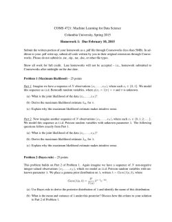
To select a suitable regression model for a query
class, we use a mixed forward and backward procedure
described below (see Figure 1). We start with the full
Start Point
1
Backward Elimination
Y = B0
+
B1 * X1
+
Basic Model
......
+
2
Forward Selection
Bn * Xn
+
.......
+
Bm * Xm
Secondary Part
Figure 1: Selection of Variables for Regression Model
basic model (3) or (4) for the query class and apply the
backward elimination procedure to drop some insignificant terms (explanatory variables) from the model.
We then apply the forward selection procedure to nd
6 The simple correlation coecient of two variables indicates
the degree of the linear relationship between the two variables.
225
ward procedure.
explanatory variables
:
Use observed data to t the full basic model
for the query class;
Calculate the standard error of estimation s;
for each variable X in VB do
Calculate the simple correlation coecient
between X and the response variable Y
end;
backward := `true';
while backward = `true' and VB 6= ; do
Let X 0 be the explanatory variable in VB
with the smallest simple correlation
coecient;
VB := VB ? f X 0 g;
Use the observed0 data to t the reduced
model with X removed;
Calculate
the standard error of estimation
s0 for0 the reduced0 model;
if s > s or j(s ? s )=sj very small then
begin
Set the reduced model as the current
model;
s := s0 ;
end
else backward := `false'
end;
forward := `true';
while forward = `true' and VS 6= ; do
for each X in VS do
Calculate the simple correlation
coecient between X and the
residuals of the current model
end;
Let X 0 be the variable with the
largest simple correlation coecient;
Use the observed 0data to t the augmented
model with X added;
Calculate
the standard error of estimation
s0 for0 the augmented
0 model;
if s > s and j(s ? s )=sj not very small
Method
begin
1.
2.
3.
4.
5.
6.
7.
8.
9.
10.
11.
12.
13.
14.
15.
16.
17.
18.
19.
20.
21.
22.
23.
5 Measures Ensuring Useful Models
To develop a useful regression model, measures
need to be taken during the analysis. Furthermore, a
developed regression model should be veried before
it is used. Improvements may be needed if the model
proves not acceptable. In this section, based on the
characteristics of the cost models for query optimization, we identify the appropriate statistical methods
and apply them to ensure the signicance of our developed cost models.
5.1 Outliers
Outliers are extreme observations. In a residual
plot, outliers are the points that lie far beyond the
scatter of the majority of points. Under the method of
least squares, a tted equation may be pulled disproportionately towards an outlying observation because
the sum of the squared deviations is minimized.
There are two possibilities for the existence of outliers. Frequently, an outlier results from a mistake or
other extraneous causes. In our application, it may be
caused by an abnormal situation in the system during
the execution of a sample query. In this case, the
outlier should be discarded. Sometimes, however, an
outlier may convey signicant information. For example, in our application, an outlier may indicate that
the underlying DBMS uses a special strategy to process the relevant sample query, which is dierent from
the one used for other queries. Since outliers represent
a few extreme cases and our objective is to derive a
cost estimation formula that is good for the majority
of queries in a query class, we simply discard the outliers and use the remaining observations to derive a
cost formula.
In a (standardized) residual plot, an outlier is usually four or more standard deviations from zero[7] .
Therefore, an observation whose residual exceeds a
certain amount of standard deviations D, such as
D = 4, can be considered as an outlier and be removed. The residuals of query observations used here
are calculated based on the full basic model since such
a model usually captures the major behavior of the nal model.
24.
25.
26.
27.
28.
then
29.
begin
30.
Set the augmented model as the
current model;
31.
VS := VS ? f X 0 g;
32.
s := s0
33.
end
34.
else forward := `false'
35. end;
36. Return the current model as the
regression model
37. end.
Since we start with the basic model, which has a
high possibility to be the appropriate model for the
given query class, the backward elimination and forward selection will most likely stop soon after they
are initiated. Therefore, our procedure is likely more
ecient than a pure forward or backward procedure.
However, in the worst case, the above procedure will
still check (k + 1) models for k potential explanatory
variables, which is the same as a pure forward or back-
5.2 Multicollinearity
When the explanatory variables are highly correlated among themselves, multicollinearity among
226
terms since the Xi;j 's in (1) are known values. In
general, regression analysis is not seriously aected by
slight to moderate departures from the assumptions.
The assumptions can be ranked in terms of the seriousness of the failure of the assumption to hold from
the most serious to the least serious as follows: assumptions 1, 2 and 3.
For our application, the observed costs of repeated
executions of a sample query have no inherent relationship with the observed costs of repeated executions of another sample query under the assumption
that the contention factors in the system are approximately stable. Hence the rst assumption should be
satised. This is a good property because the violation of assumption 1 is the most serious to a regression
model.
However, the variance of the observed costs of repeated executions of a sample query may increase
with the level (magnitude) of query cost. This is because the execution of a sample query with longer time
(larger cost) may suer more disturbances in the system than the execution of a sample query with shorter
time. Thus assumption 2 may be violated in our regression models. Furthermore, the observed costs of
repeated executions of a sample query may not follow
the normal distribution; i.e., assumption 3 may not
hold either. The observed costs are usually skewed to
the right because the observed costs stay at a stable
level for most time and become larger from time to
time when disturbances occur in the system.
Since the uncorrelation assumption is rarely violated in our application, it is not checked by our regression analysis program. For the normality assumption,
many studies have shown that regression analysis is robust to it[7; 9] ; that is, the technique will give usable
results even if this assumption is not satised. In fact,
the normality assumption is not required to obtain the
point estimates of Bbi 's, Yb and s. This assumption is
required only when constructing condence intervals
and hypothesis-testing decision rules. In our application, we will not construct condence intervals, and
the only hypothesis-test that needs the normality assumption is the F -test which will be discussed later.
Like many other statistical applications, if only the
normality assumption is violated, we choose to ignore
this violation. Thus, the normality assumption is not
checked by our regression analysis program either.
When the assumption of equal variances is violated,
a correction measure is usually taken to eliminate or
reduce the violation. Before a correction measure is
given, let us rst discuss how to test for the violation
of equal variances.
them is said to exist. The presence of multicollinearity does not, in general, inhibit our ability to obtain
a good t nor does it tend to aect predictions of
new observations, provided these predictions are made
within the region of observations. However, the estimated regression coecients tend to have large sampling variability. To make reasonable predictions beyond the region of observations and obtain more precise information about the true regression coecients,
it is better to avoid multicollinearity among explanatory variables.
A method to detect the presence of multicollinearity that is widely used is by means of variance ination
factors. These factors measure how much the variances of the estimated regression coecients are inated as compared to when the independent variables
are not linearly related. If Rj2 is the coecient of total determination that results when the explanatory
variable Xj is regressed against all the other explanatory variables, the variance ination factor for Xj is
dened as
V IF (Xj ) = 1=(1 ? Rj2 ) :
It is clear that if Xj has a strong linear relationship
with the other explanatory variables, Rj2 is close to 1
and V IF (Xj ) is large.
To avoid multicollinearity, we use the reciprocal of
a variance ination factor to detect instances where
an explanatory variable should not be allowed into
the tted regression model because of excessively high
interdependence between this variable and other explanatory variables in the model.
More specically, the set VB of basic explanatory
variables used by Algorithm 4.1 is formed as follows.
At the beginning, VB only contains the basic explanatory variable which has the highest simple correlation
coecient with the response variable Y . Then the
variable Xj which has the next highest simple correlation coecient with Y is entered into VB if 1=V IF (Xj )
is not too small. This procedure continues until all
possible basic explanatory variables are considered.
Similarly, when Algorithm 4.1 selects additional benecial variables from VS for the model, any variable Xj
whose 1=V IF (Xj ) is too small is skipped.
5.3 Validation of Model Assumptions
Usually, three assumptions of a regression model (1)
need to be checked: 1. uncorrelation of error terms;
2. equal variance of error terms; and 3. normal distribution of error terms.
Note that the dependent random variables Yi 's
should satisfy the same assumptions as their error
227
Assuming that a regression model is proper to t
sample observations, the sampled residuals should reect the assumptions on the error terms. We can,
therefore, use the sampled residuals to check the assumptions. There are two ways in which the sampled
residuals can be used to check the assumptions[7; 9] :
residual plots and statistical tests. The former is subjective, while the latter is objective. Since we try to
develop a program to test assumption 2 automatically,
we employ the latter.
As mentioned before, if the assumption of equal
variances is violated in our application, variances typically increase with the level of the response variable.
In this case, the absolute values of the residuals usually have a signicant correlation with the tted values
of the response variable. A simple test for the correlation between two random variables u and w when the
bivariate distribution is unknown is to use Spearman's
rank correlation coecient[9; 12] , which is dened as
rs = 1 ? 6
squares. The idea is to provide diering weights in
(1); that is,
LSw =
i
i=1
i
i
0 + B1 Xi;1 + B2 Xi;2
+ + Bk Xi;k )]2 ;
where wi is the weight for the i-th Y observation.
The values for Bj 's to minimize LSw is to be found.
Least squares theory states that the weights wi 's are
inversely proportional to the variances i2 's of the error terms. Thus an observation Yi that has a large
variance receives less weight than another observation
that has a smaller variance. The (weighted) variances
of error terms tend to be equalized.
Unfortunately, one rarely has knowledge of the variances i2 's. To estimate the weights, we do the following. The sample data is used to obtain the tted regression function and residuals by ordinary least
squares rst. The cases are then placed into a small
number of groups according to level of the tted value.
The variance of the residuals is calculated for each
group. Every Y observation in a group receives a
weight which is the reciprocal of the estimated variance for that group.
Moreover, we use the results of weighted least
squares to re-estimate the weights and obtain a new
weighted least squares t. This procedure is continued until no substantial changes in the tted regression function take place or too many iterations occur.
In the latter case, the tted regression function with
the smallest Spearman's rank correlation coecient is
chosen. This procedure is called an iterative weighted
least squares procedure.
Xn [r(u ) ? r(w )]=[n(n2 ? 1)];
i=1
Xn w [Y ? (B
i
where r(ui ) and r(wi ) are the ranks of the values ui
and wi of u and w, respectively. The null and alternate
hypotheses are as follows:
H0 : The values of u and w are uncorrelated.
HA : Either there is a tendency for larger values of u
to be paired with the larger values of w, or there
is a tendency for smaller values of u to be paired
with larger values of w.
The decision rule at the signicance level is:
5.4 Testing Signicance of Regression
Model
If 1?=2 rs =2 , conclude H0 .
As mentioned previously, to evaluate the goodness
of the developed regression model, two descriptive
measures are used: the standard error of estimation
and the coecient of multiple determination. A good
regression model is evidenced by a small standard error of estimation and a high coecient of multiple
determination.
The signicance of the developed model can be
further tested by using the F -test[7; 9] . The F -test
was derived under the normality assumption. However, there is some evidence that non-normality usually does not distort the conclusions too seriously[12] .
In general, the F -test under the normality assumption is asymptotically (i.e., with suciently large samples) valid when the error terms are not normally
If rs < 1?=2 or rs > =2 , conclude HA .
The critical values =2 = ?1?=2 can be found in [9].
If HA is concluded for the absolute residuals and tted
values, the assumption of equal variances is violated.
If the assumption of equal variances is violated, the
estimates given by the corresponding regression model
will not have the maximum precision[2] . Since the estimation precision requirement is not high for query
optimization, the violation of this assumption can be
tolerated to a certain degree. However, if the assumption of equal variances is severely violated, account
should be taken of this in tting the model.
A useful tool to remedy the violation of the equal
variances assumption is the method of weighted least
228
Class
Gu1
Gu2
Gu3
Gj1
Gj2
Gj3
Characteristics of Queries in the Class
Likely Access Method
unary queries whose qualications have at least one conjunct Ri :an = C
where Ri :an is indexed
unary queries that are not in Gu1 and whose qualications have at least one
conjunct Ri :an C where Ri :an is indexed and 2 f<; ; >; ; g
unary queries that are not in Gu1 or Gu2
join queries whose qualications have at least one conjunct Ri :an = Rj :am
where either Ri :an or Rj :am (or both) is indexed
join queries that are not in Gj1 and whose qualications have at least one
index-usable conjunct for one or both operand tables
join queries that are not in Gj1 or Gj2
index scan method
with a key value
index scan method
with a range
sequential scan method
index join method
nested-loop join method
with index reduction rst
sort-merge join method
Table 1: Considered Query Classes
distributed[1] . Therefore, F -test is adopted in our application to test the signicance of a regression model
although the error terms may not follow the normality
assumption.
Gu1 when queries can be executed very fast, i.e.,
small-cost queries, due to their ecient access
methods and small result tables.
The standard errors of estimation for the cost
models are acceptable, compared with the magnitudes of the relevant average observed costs of
the sample queries.
6 Experiments
To verify the feasibility of the presented statistical
procedure, experiments were conducted within a multidatabase system prototype, called CORDS-MDBS.
Three commercial DBMSs, i.e., ORACLE 7.0, EMPRESS 4.6 and DB2/6000 1.1.0, were used as local
DBMSs in the experiments. All the local DBMSs were
run on IBM RS/6000 model 220 machines. Due to the
limitation of the paper length, only the experimental
results on ORACLE 7.0 are reported in this paper.
The experiments on the other systems demonstrated
similar results.
The experiments were conducted in a system environment where the contention factors were approximately stable. For example, they were performed
during midnights and weekends when there was no
or little interference from other users in the systems.
However, occasional interference from other users still
existed since the systems were shared resources.
Queries for each local database system were classied according to the query sampling method. The
considered query classes7 are given in table 1. Sample queries are then drawn from each query class and
performed on the three local database systems. Their
observed costs are used to derive cost models for the
relevant query classes by the statistical procedure introduced in the previous sections.
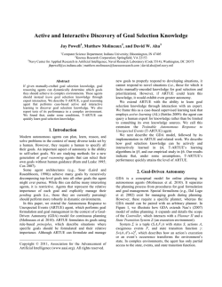
Tables 2 and 3 show the derived cost models and
the relevant statistical measures. It can be seen that:
The statistical F-tests at the signicance level
= 0:01 show that all derived cost models are
useful for estimating the costs of queries in the
relevant query classes.
The statistical hypothesis tests for the Spear-
man's rank correlation coecients at the significance level = 0:01 show that there is no strong
evidence indicating the violation of equal variances assumption for all derived cost models after using the method of weighted least squares if
needed.
Derivations of most8 cost models require the
method of weighted least squares, which implies
that the error terms of the original regression
model (using the regular least squares) violate the
assumption of equal variances in most cases.
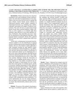
In summary, the statistical procedure derived useful
cost models. Figure 2 shows a typical comparison between the observed costs and our estimated costs for
some test queries.
As mentioned, the experimental results show that
small-cost queries often have worse estimated costs
than large-cost queries. This observation coincides
with Du et al.'s observation for their calibration
method. The reason for this phenomenon is that (1)
a cost model is usually dominated by large costs used
to derive it, while the small costs may not follow the
Most cost models capture over 90% variability
in query cost, from observing the coecients of
total determination. The only exception is for
7
Some unreported cost models for other local database systems in the experiments did not require the method of weighted
least squares.
8
Only equijoin queries were considered.
229
query
class
Cost Estimation Formula
0.866475e-1 + 0.177483e-2 TNU + 0.926299e-2 RNU + 0.443237e-6 ZU
0.354301 + 0.105255e-2 TNU + 0.32336e-2 RNU + 0.852187e-4 RZU
0.16555 + 0.149208e-3 NU + 0.307219e-2 RNU + 0.105712e-3 RZU
0.192209 + 0.161011e-2 TNJ 2 + 0.573257e-7 TNJ 12 + 0.426256e-2 RNJ
0.176158 + 0.951479e-3 TNJ 12
-0.236703e-1 + 0.143572e-3 NJ 2 + 0.61871e-3 TNJ 1 + 0.680628e-3 TNJ 2
+ 0.399927e-6 TNJ 12 + 0.316129e-2 RNJ
Gu1
Gu2
Gu3
Gj 1
Gj 2
Gj 3
Table 2: Derived Cost Formulas for Query Classes on ORACLE 7.0
query
class
Gu1
Gu2
Gu3
Gj 1
Gj 2
Gj 3
coecient
of multiple
determination
0.65675
0.96751
0.99810
0.98992
0.92457
0.97670
standard
error of
estimation
0.10578
0.27357e+1
0.87345
0.14961e+1
0.51609e+3
0.15275e+1
average
cost
(sec.)
0.20406
0.11360e+2
0.13595e+2
0.60868e+1
0.75323e+3
0.71334e+1
F-statistic
(critical value
at = 0:01)
56.76 (> 3.97)
1161.46 (> 4.29)
15397.70 (> 3.97)
3732.28 (> 4.28)
1483.19 (> 7.06)
980.69 (> 3.52)
Spearman's rank
correlation (critical
value at = 0:01)
0.54266e-1 (< 0.24292)
0.21032 (< 0.21270)
0.20930e-1 (< 0.24425)
0.61343e-1 (< 0.21541)
0.74099e-1 (< 0.21095)
0.13307 (< 0.21095)
weighted
least
square?
yes
yes
yes
yes
yes
yes
Table 3: Statistical Measures for Cost Formulas on ORACLE 7.0
(a) rening the query classication according to the
sizes of result tables; and/or (b) performing a sample
query multiple times and using the average of observed
costs to derive a cost model; and/or (c) including in
the cost model more explanatory variables if available,
such as buer sizes, and distributions of data in a disk
space.
Fortunately, estimating the costs of small-cost
queries is not as important as estimating the costs of
large-cost queries in query optimization because it is
more important to identify large-cost queries so that
\bad" execution plans could be avoided.
same model because dierent buering and processing
strategies may be used for the small-cost queries; (2) a
small cost can be greatly aected by some contention
factors, such as available buer space and the number
of current processes; (3) initialization costs, distribution of data over a disk space and some other factors,
which may not be important for large-cost queries,
could have major impact on the costs of small-cost
queries.
70
solid line --- estimated cost
Cost (Elapse Time in Sec.)
60
dotted line --- observed cost
+
7 Conclusion
50
Today's organizations have increasing requirements
for tools that support global access to information
stored in distributed, heterogeneous, autonomous data
repositories. A multidatabase system is such a tool
that integrates information from multiple pre-existing
local databases. To process a global query eciently
in an MDBS, global query optimization is required.
A major challenge for performing global query optimization in an MDBS is that some desired local cost
information may not be available at the global level.
Without knowing how eciently local queries can be
executed, it is dicult for the global query optimizer
to choose a good decomposition for the given global
query.
To tackle this challenge, a feasible statistical procedure for deriving local cost models for a local database
system is presented in this paper. Local queries are
grouped into homogeneous classes. A cost model is
developed for each query class. The development of
40
30
++
+
+
20
+ +
+
+ +
++
10 + ++
+ +++
+ +
+
+++++
+
+
++
+++++ ++
++++++
+
+
++
+
0
0
0.2
+
++
+ +
+
+
+
0.4
0.6
0.8
1
Result Table Cardinality
1.2
1.4
1.6
1.8
x10 4
Figure 2: Observed and Estimated Costs for Test
Queries in Gj3 on ORACLE
Since the causes of this problem are usually uncontrollable and related to implementation details of the
underlying local database system, it is hard to completely solve this problem at the global level in an
MDBS. However, this problem could be mitigated by
230
cost models are base on multiple regression analysis.
Each cost model is divided into two parts: a basic
model and a secondary part. The basic model is based
on some existing cost models in DBMSs and used to
capture the major performance behavior of queries.
The secondary part is used to improve the basic model.
Potential explanatory variables that can be included
in each part of a cost model are identied. A backward
procedure is used to eliminate insignicant variables
from the basic model for a cost model. A forward
procedure is used to add signicant variables to the
secondary part of a cost model. Such a mixed forward
and backward procedure can select proper variables
for a cost model eciently.
During the regression analysis, outliers are removed
from the sample data. Multicollinearity is discovered
by using the variance ination factor and prevented
by excluding variables with larger variance ination
factors. Violation of the equal variance assumption is
detected by using Spearman's rank correlation coecient and remedied by using an iterative weighted least
squares procedure. The signicance of a cost model is
checked by the standard error of estimation, the coecient of multiple determination, and F-test. These
measures ensure that a developed cost model is useful.
The experimental results demonstrated that the
presented statistical procedure can build useful cost
models for local database systems in an MDBS.
The presented procedure introduces a promising
method to estimate local cost parameters in an MDBS
or a distributed information system. We plan to investigate the feasibility of this method for non-relational
local database systems in an MDBS in the future.
[6] H. Lu, B.-C. Ooi, and C.-H. Goh. On global multidatabase query optimization. SIGMOD Record,
21(4):6{11, Dec. 1992.
[7] J. Neter, W. Wasserman, and M. H. Kutner. Applied Linear Statistical Models, 3rd Ed. Richard D.
Irwin, Inc., 1990.
[8] F. Olken and D. Rotem. Simple random sampling
from relational databases. In Proc. of 12th VLDB,
pp 160{9, 1986.
[9] R. C. Pfaenberger and J. H. Patterson. Statistical
Methods for Business and Economics. Richard D.
Irwin, Inc., 1987.
[10] P. G. Selinger et al. Access path selection in relational database management systems. In Proc. of
ACM SIGMOD, pp 23{34, 1979.
[11] G. P. Shapiro and C. Connel. Accurate estimation
of the number of tuples satisfying a condition. In
Proc. of SIGMOD, pp 256{76, 1984.
[12] G. W. Snedecor and W. G. Cochran. Statistical
Methods, 6th Ed. The Iowa State university Press,
1967.
[13] Qiang Zhu. Query optimization in multidatabase
systems. In Proc. of the 1992 IBM CAS Conf.,
vol.II, pp 111{27, Toronto, Canada, Nov. 1992.
[14] Qiang Zhu and P.-
A. Larson. A query sampling
method for estimating local cost parameters in a
multidatabase system. In Proc. of the 10th IEEE
Int'l Conf. on Data Eng., pp 144{53, Houston,
Texas, Feb. 1994.
[15] Qiang Zhu and P.-
A. Larson. Establishing a
fuzzy cost model for query optimization in a multidatabase system. In Proc. of the 27th IEEE/ACM
Hawaii Int'l Conf. on Sys. Sci., pp 263-72, Maui,
Hawaii, Jan. 1994.
[16] Qiang Zhu and P.-
A. Larson. Query optimization
using fuzzy set theory for a multidatabase system.
In Proc. of the 1993 IBM CAS Conf., pp 848{59,
Toronto, Canada, Oct. 1993.
References
[1] S. F. Arnold. The Theory of Linear Models and
Multivariate Analysis. John Wiley & Sons, Inc.,
1981.
[2] S. Chatterjee and B. Price. Regression Analysis by
Example, 2nd Ed. John Wiley & Sons, Inc., 1991.
[3] W. Du, R. Krishnamurthy, and M. C. Shan. Query
optimization in heterogeneous DBMS. In Proc. of
VLDB, pp 277{91, 1992.
[4] M. Jarke and J. Koch. Query optimization in
database systems. Computing Surveys, 16(2):111{
152, June 1984.
[5] R. J. Lipton and J. F. Naughton. Practical selectivity estimation through adaptive sampling. In
Proc. of SIGMOD, pp 1{11, 1990.
231