1. No category

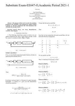
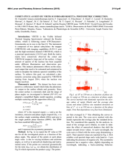
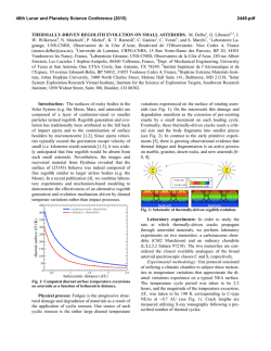
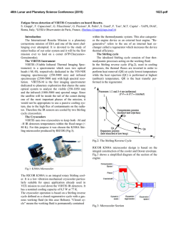
Universidad Nacional de Ingeniería
Facultad de Ingeniería Eléctrica y Electrónica
“SOLUCIONARIO EXAMEN PARCIAL”
Sistemas de Control I (EE-647O)
(Ciclo académico 2021-1)
Ccoicca Leiva Jhonathan José
[email protected]
Abstract- The document contains the solution for the final exam of
Control I.
Solution:
a)
I.
I disagree with the L.G.R. shown:
INTRODUCTION
In this work we will appreciate the use of the concepts and
methods provided in class for the analysis and resolution of
exam final of control system I, where the following topics were
presented: the geometric place of the roots, the Routh-Hurwitz
stability criterion and bode diagrams.
.
II. PROBLEMS SOLVE
A. Problem 1
A student in the Control Systems I course is asked to determine
the L.G.R. of a certain open-loop system (GH(s)), which is
represented by the following graph, and then it is asked:
a)
Do you agree with the L.G.R. shown?, If there is an error in
its drawing, where would the error made by the student be
when drawing the L.G.R.? Agree or not, how do you come to
that conclusion?
b)
According to your previous answer, what would be the
stroke of the L.G.R. with the poles (x) and zeros (o) already
located in the diagram?
c)
With all the information obtained, what is the open-loop
transfer function (GH(s)) represented in the L.G.R.?
Fig. 2 Place where the error is found.
We notice that the only possibility is that they are located in
the figure 2.2 are two poles and in the direction shown one
pole would be looking for another pole and that should not
happen in the L.G.R.
Fig. 1 L.G.R.
b)
The LGR will be:
B. Problem 2
The following figure presents a block diagram of a
specific control system.
Fig. 5 Block diagram.
So, you are asked what values can the open loop gain (K) take,
so that the system is stable?
Fig. 3 The corrected L.G.R.
c)
Solution:
To find out if the system is stable we apply the Routh-Hurwitz
criterion.
The open-loop transfer function will be:
( )
(
(
)(
)
)(
)(
)
Doing:
Then, characteristic equation in closed loop:
( )
We will simulate the open-loop transfer function:
(
(
(
)(
)
)
)
(
)
(
)
We verify that all the coefficients of the equation meet the
following condition:
 They have the same sign.
0…(1)
Fig. 4 LGR graph obtained by simulation with Matlab live.
⇒ k’ ∈ ℝ+ ⇒ ’ >
From some of the traces in the magnitude diagram (not all), you
are asked to identify:
Where:

|
a) What elements does the plant have and where are they
located?
b) What is the static gain of the plant?
|
Solution:
a) Identifying the elements that the plant has in the Bode
diagram:


|
|
|
(
⇒
|
)
Fig. 7. Bode diagram with the identified elements.
We notice that all the terms in the first column of Routh's table
are positive, so the system is stable.
In (1):
Then, the open-loop transfer function would be:
( )
⇒
C. Problem 3
For the frequency response shown below, it belongs to a
negative and unit feedback plant.
(
(
)(
)
)(
)
Finding k:
…( )
Then:
(
( )(
)
)(
…( )
)
(1)= (2):
( )
(
(
)(
)
)(
)
b)
( )
( )(
)(
)
REFERENCES
Fig. 6. Bode Diagram
[1] K. Ogata, Ingeniería de control moderna, 5th ed, Madrid 2010, pp. 29-164.
[2] C.Chen, Analog and digital control system design, 3rd ed., New York:
McGraw-Hill Book Company, 1993, pp.116.
[3] Dorf, R. C., and R. H. Bishop, Modern Control Systems, 9th ed. Upper
Saddle River, NJ: Prentice Hall,2001., pp. 209-223.