1. No category

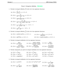
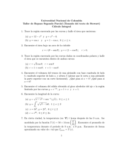
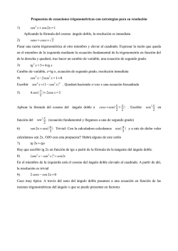
TRA NSFORMACIO N ES LIN EA LES II
C o m p uta c i ó n G r á fica
Rotaciones
Transformación lineal que preserva producto punto entre vectores.
Transforma bases de mano derecha a bases de mano derecha.
En 3D, cada rotación fija un eje de rotación y rota por un ángulo alrededor de ese eje.
Vemos el caso 2D. Consideramo un vector:
~v =
h
b~1
i x
b~2
y
t
~
Suponemos que b es una base ortonormal de mano derecha en 2D.
v, ✓ grados en sentido anti-horario alrededor del origen.
Supongamos que queremos rotar ~
Las coordenadas
⇥
x
0
y
0
⇤t
del vector rotado se pueden calcular:
0
x = x cos ✓
y sin ✓
0
y = x sin ✓ + y cos ✓
S.J. Gortler. Foundations of 3D Computer Graphics. MIT Press. 2012.
COMPUTACIÓN GRÁFICA
|
TRANSFORMACIONES LINEALES II
|
ENERO-JUNIO 2015
|
11/02/2015
Rotaciones: 2D
Que se puede escribir:
h
b~1
i x
b~2
y
)
h
)
h
b~1
i  cos ✓
b~2
sin ✓
sin ✓
cos ✓
b~1
i  cos ✓
b~2
sin ✓
sin ✓
cos ✓

x
y
También podemos rotar una base:
h
b~1
b~2
i
S.J. Gortler. Foundations of 3D Computer Graphics. MIT Press. 2012.
COMPUTACIÓN GRÁFICA
|
TRANSFORMACIONES LINEALES II
|
ENERO-JUNIO 2015
|
11/02/2015
Rotaciones: 3D
Usando un sistema coordenado de mano derecha, una rotación de un vector por θ grados alrededor del
eje z de la base se expresa:
2
3
h
i x
h
b~1 b~2 b~3 4 y 5 ) b~1
z
b~2
b~3
i
2
cos ✓
4 sin ✓
0
sin ✓
cos ✓
0
32
0
x
0 54 y 5
1
z
Una rotación de un vector por θ grados alrededor del eje x de la base se expresa:
h
b~1
b~2
b~3
i
2
3
x
h
4 y 5 ) b~1
z
b~2
b~3
i
2
1
0
4 0 cos ✓
0 sin ✓
3
32
3
0
x
sin ✓ 5 4 y 5
cos ✓
z
S.J. Gortler. Foundations of 3D Computer Graphics. MIT Press. 2012.
COMPUTACIÓN GRÁFICA
|
TRANSFORMACIONES LINEALES II
|
ENERO-JUNIO 2015
|
11/02/2015
Rotaciones: 3D
Una rotación de un vector por θ grados alrededor del eje y de la base se expresa:
h
b~1
b~2
b~3
i
2
3
x
h
4 y 5 ) b~1
z
b~2
b~3
i
2
cos ✓
4
0
sin ✓
0
1
0
32
3
sin ✓
x
0 54 y 5
cos ✓
z
La composición de rotaciones resulta en otra rotación.
Podemos tener una rotación arbitraria aplicando una rotación alrededor del eje-x, seguida de una alrededor del eje-y
y luego una alrededor del eje-z.
Las cantidades angulares de las tres rotaciones se conocen como ángulos de Euler xyz. (roll-pitch-yaw)
S.J. Gortler. Foundations of 3D Computer Graphics. MIT Press. 2012.
COMPUTACIÓN GRÁFICA
|
TRANSFORMACIONES LINEALES II
|
ENERO-JUNIO 2015
|
11/02/2015
Matrices de rotación R
Matrices cuadradas, con elementos reales.
T
-1
Matrices ortogonales: R = R y det R =1.
Si incluimos aquellas cuyo det R = -1 incluimos también las reflexiones.
El conjunto de las matrices de tamaño n con det R = +1 forman un grupo llamado ortogonal especial SO(n).
En 3D es SO(3).
ortogonal especial
(1) Vectores renglón unitarios
(2) Vectores renglón perpendiculares entre si (producto punto es cero)
(3) Los vectores columna también verifican las propiedades (1) y (2).
S.J. Gortler. Foundations of 3D Computer Graphics. MIT Press. 2012.
COMPUTACIÓN GRÁFICA
|
TRANSFORMACIONES LINEALES II
|
ENERO-JUNIO 2015
|
11/02/2015
Ax is-a ngle
Otra forma de representar una rotación arbitraria es tomar un vector unitario ~k como eje
de rotación y aplicar directamente una rotación de θ radianes alrededor de éste.
~k =
2
2
kx v
⇥
+c
~k = 4 ky kx v + kz s
kz kx v ky s
kx
ky
⇤t
kz
k x ky v kz s
2
ky v + c
kz ky v + kx s
c := cos ✓
s := sin ✓
3
kx kz v + ky s
ky k z v k x s 5
2
kz v + c
v := 1
c
S.J. Gortler. Foundations of 3D Computer Graphics. MIT Press. 2012.
COMPUTACIÓN GRÁFICA
|
TRANSFORMACIONES LINEALES II
|
ENERO-JUNIO 2015
|
11/02/2015
Rotaciones
Dos rotaciones alrededor de ejes diferentes no conmutan entre sí.
Cuando componemos dos rotaciones alrededor de dos ejes diferentes tenemos una rotación alrededor de un tercer eje.
Diferentes parametrizaciones de rotaciones:
Matrices de rotación
Axis-angle
Ángulos de Euler
Cuaternios
Mapa exponencial
S.J. Gortler. Foundations of 3D Computer Graphics. MIT Press. 2012.
COMPUTACIÓN GRÁFICA
|
TRANSFORMACIONES LINEALES II
|
ENERO-JUNIO 2015
|
11/02/2015
Esca la m ientos
Para escalar un vector por un factor s podemos usar:
~v =
h
b~1
b~2
b~3
i
2
3
x
h
4 y 5 ) b~1
z
b~2
b~3
i
2
sx
4 0
0
32
0
sy
0
3
0
x
0 54 y 5
sz
z
sx = sy = sz : escalamiento uniforme.
sx ≠ sy ≠ sz : escalamiento diferencial.
S.J. Gortler. Foundations of 3D Computer Graphics. MIT Press. 2012.
COMPUTACIÓN GRÁFICA
|
TRANSFORMACIONES LINEALES II
|
ENERO-JUNIO 2015
|
11/02/2015
Ciza lla m iento (Shea r)
Para cizallar un vector alrededor del eje-z:
~v =
h
b~1
b~2
b~3
2
3
x
h
4 y 5 ) b~1
z
i
b~2
b~3
i
2
1
4 0
0
32
0
1
0
a
x
b 54 y 5
1
z
http://140.129.20.249/~jmchen/cg/docs/rendering%20pipeline/rendering/transforms.html
COMPUTACIÓN GRÁFICA
|
TRANSFORMACIONES LINEALES II
|
ENERO-JUNIO 2015
3
|
11/02/2015
Tra nsformaciones Linea les
De cuerpos rígidos:
secuencia arbitraria de translaciones y rotaciones.
preservan paralelismo, ángulos y longitudes.
Afines:
secuencia arbitraria de rotaciones, translaciones, escalamientos y cizallamientos (shear).
preserva paralelismo.
COMPUTACIÓN GRÁFICA
|
TRANSFORMACIONES LINEALES II
|
ENERO-JUNIO 2015
|
11/02/2015
Coordenadas Homogéneas
Coordenadas homogéneas o coordenadas proyectivas.
Introducidas por August Ferdinand Möbius en 1827.
Sistema de coordenadas utilizado en geometría proyectiva, como las
coordenadas cartesianas se usan en geometría Euclideana.
En CG permiten que las operaciones como translación, rotación,
escalamiento, proyecciones perspectivas se implementen con matrices.
COMPUTACIÓN GRÁFICA
|
TRANSFORMACIONES LINEALES II
|
ENERO-JUNIO 2015
|
11/02/2015
Features of the Beamer Class
⇥
dx
2
P = T + P, donde P y P son puntos en R y T =
.
dy
⇥
sx 0
2
⇤
⌅
P = S · P, donde P ydP son puntos en R y S =
.
x
0 sy
2
P = T + P, donde P y P son puntos en R y T =
.
dy
2 y
P
=
R
·
P,
donde
P
y
P
son
puntos
en
R
Permiten tratar a las transformaciones de
⇤
⇥ ⌅
s
0
cos
sin
x
2
Features
manera
consistente.
P of
= Sthe
· P,Beamer
donde P yClass
P son puntos
.
R =en R y S =
.
sin
cos 0 sy
(x, yen
, WR)2con
=⇤R · P, donde
P y⌅tripletas
P son puntos
y W ⇥= 0.
Un punto seP representa
con
W
P
cos
sin
que son múltiplos
entre si. .
R=
sin
cos
⇤
⌅
dx
2
(tx,
ty
,
tW
)
con
t
=
⇥
0.
P = T +⇥P, donde P y P son puntos en R y T =
.
dy
y
x
⇤
⌅
W , W , 1 con W ⇥= 0.
plano
W=1
que es una línea en un espacio 3D.
sx 0
2
P = S · P, donde P y P son puntos en R y S =
.
0 sy
Coordenadas Homogéneas
Coordenadas
cartesianas
del
punto
P =⇤R · P, donde P y⌅ P son puntos en R2 y
homogéneo:
cos
sin
R=
(x, y, 0) ?
.
sin
cos
⇥
y
x
W , W , 1 con W ⇥= 0.
y
puntos al infinito en dirección (x, y).
13
x
Coordenadas homogéneas
Al menos una de las coordenadas homogéneas debe ser diferente a cero.
Si la coordenada W es diferente a cero podemos dividir entre ella:
(x,y,W) representa el mismo punto que (x/W, y/W, 1).
Cuando W es diferente a cero hacemos esta división y los números x/W, y/
W se llaman coordenadas Cartesianas del punto homogéneo.
Los puntos con W=0 se llaman puntos en el infinito.
COMPUTACIÓN GRÁFICA
|
TRANSFORMACIONES LINEALES II
|
ENERO-JUNIO 2015
|
11/02/2015
sx 0
P = S · P, donde P y P son puntos en
yS=
.
2
P = S · P, donde P y P son puntos en
0 Rsy y S =
R2
2 y
P =⇤R · P,
donde
P
y
P
son
puntos
en
R
Translación
en donde
coordenadas
P y⌅ P son puntos en
P =⇤R⌅· P,
cos
sin
cos
sin
R=
.
R
.
sin
cos=homogéneas
sin
cos
(x, y , 0) con t ⇥= 0.
(x, y , 0) con t ⇥= 0.
⇥
y
x
⇥
,
,
1
con
W
=
⇥
0.
y
x
W W
0.
⌃
W , W , 1 con W ⇥= ⇧
1 0 dx ⇧
1
P = T (dx , dy ) · P con T (dx , dy ) = ⌥ 0 1 dy .⌥
P = T (dx , dy ) · P con T (dx , dy ) = 0
Features Features
of the Beamer
Class
0 0 1
of
the
Beamer
Class
0
Features of the Beamer Class
sx
0
R2 y
⌃
0 dx
1 dy .
0 1
⇧
⌃
1 0 dx
P = T (dx1 x2 , dy1 y2 ) · P con T (dx , dy ) = ⌥ 0 1 dy .
0 0 1
T (dx1 x2 , dy1 yT2 )(d= T ,(ddx2 , d)y2=) ·TT(d
(dx1, ,ddy1))· T (d , d )
T (dx1 x2 , dxy1 x1 y2 2⇥) y=1 y2T (dx2 , dyx2 2) ·⇥Ty2(dx1 , dyx1 1) y1
1 0 dx2 1 0 1⇥d 0 ⇥dx1 1 0 ⇥d ⇥
x2 1 0 d
x1
1
0
d
x
x
dy2⇤ ⌅0· ⇤12 0 d 1 ⌅d·y1⇤ ⌅0 11 d ⌅
=⇤ 0 1 =
⇤ 0 1 dy2 ⌅ y· 2⇤ 0 1 dy1 ⌅ y1
=
0 0 1 0 0 0 10 1 0 0 1
0 0 1
0 0 1
⇥
1 0 dx1 +1dx20 dx +⇥dx ⇥
1
2
1
0
d
+
d
x
x
1
2
⌅
⇤
dy1⇤+0dy21 d. y + dy ⌅ .
= 0 1 =
⇤ 0 1 dy1 + d1y2 ⌅ . 2
=
0 0
10 0
1
0 0
1
COMPUTACIÓN GRÁFICA
|
TRANSFORMACIONES LINEALES II
|
ENERO-JUNIO 2015
|
11/02/2015
0
sy
.
Escalamiento en coordenadas
homogéneas
Escalamiento
Escalamiento
Escalamiento
Escalamiento
P = S(sx , Escalamiento
sy ) · P con S(sx , sy ) = ⇤
⇥
sx 0 0
0 sy 0 ⌅.
⇥
sx ⇥0 0
0 0 1
0 ⌅.
P = S(sx , sy ) · P con S(sx , sys)x = 0⇤ 00 sy ⇥
1
0
d
⇤
⌅
0 sy 00 0. xsx 1 0
P = S(sx , sy ) · P con S(sx , sy ) =
⇤
⌅
⇤
0
1
d
P = T (dx1 x2 , dy1 y2 )P· P=con
(d
,
d
)
=
.sy
0
S(sT
,
s
)
·
P
con
S(s
,
s
)
=
y
x
x
y
y
1 2 0 x 0y 1
x y 1 2
sx 0
P = S(sx1 x2 , sy1 y2 ) · P
0 0 ⇤ 10 0
0 sy
P
=2 )S(s
, sy ) · P con S(sx , sy ) =
P = S(s
,
s
·
P
x
x
x
y
y
1
2
1
T
(d
,
d
)
=
T
(d
,
d
)
·
T
(d
,
d
).
x
x
y
y
x
y
x
y
1
2
1
2
2
2
1
1
T
(dxy11,yd2 y)1·).P
T (dx1 x2 , dy1 y2 ) = T (d
Px2 ,=dyS(s
2 ) ·x⇥
0 0
⇥
1 x2 , s
S(sx1 x2 , sy1⇥y2 )1= 0S(sdx2 , sy2 ) ⇥
· S(s
,
s
).
x1 0 y1d
1
x
x1
2d
⇥
⇥
1 0 dx2
1
0
S(sx=1 x2S(s
, syx1⌅
S(s
, sy2 ) ·⌅S(sx1 , sy1 ).
xy1x2 ), =
P
s
)
·
x2P
y
y
1
2
1
2
⇤
⇤
1 =0⌅ d0⇤
d0x1⇥ 1 dy1
·
x2 1 dy21 0
⇥
⇤
⌅
= 0 1⇤ dy2 · 0⌅ s1⇤ dy01 0 ⌅ s
0 x1 0, sy1 ).
,
s
)
=
S(s
,
s
x1
x21) · S(s
2
0
1
d
= 0 1 d0yS(s
·
x
x
y
y
x
y
0
0
0
1
1
2
1
2
2
y
2
1
0
0
1
0 0 1
⇥
⇥
⇤
⌅
⇤
⌅
⇥
0
s
0
0
s
0
=
·
y
y
2
1
0 0 11 ⇥
0+0d
0 01
sx1 0 0
0 sdx2x1⇥
x
2
1 0 dx1 + dx=
0
0
1
0
0
1
⇤
⌅
⇤
⌅
2
0
s
0
0
s
0
·
⌅
⇤
x = y : escalamiento uniforme.
y
y
1
0
d
+
d
1
1 xd2y1 + d2 y2 . ⇥
= 0x1 ⌅
⇤
= 0 1⇤ dy1 + dy2 . 10 ⌅
0 1
x ≠ y : escalamiento diferencial.
= 0 1 d0y1 +
0 dy2 01.0dx1 1+ dx2 0
0 0
1 = ⇤ 0 1 d + d ⌅. ⇥
0 0
1 sx1 · sx2 y1 0 y2 0
0 ⌅.
s1 ·s
= ⇤ 0 00
y2
y1
0
COMPUTACIÓN GRÁFICA
|
TRANSFORMACIONES LINEALES II
0
|
1
ENERO-JUNIO 2015
|
11/02/2015
⇥
0
⇥
⌅.
0
0
01 ⌅.
1
Rotación en coordenadas
homogéneas
Rotación
Alrededor del origen.
Rotación
cos
P = R( ) · P con R( ) = ⇤ sin
0
sin
cos
0
P = S(sx1 x2 , sy1 y2 ) · P
⇥
0
0 ⌅.
1
S(sx1 x2 , sy1 y2 ) = S(sx2 , sy2 ) · S(sx1 , sy1 ).
⇥
⇥
⇥
cos
sin
0sx2 0 0
sx1 0 0
cos= ⇤ 00⌅. sy2 0 ⌅ · ⇤ 0 sy1 0 ⌅
P = R( ) · P con R( ) = ⇤ sin
0
0
10
0 1
0
0 1
⇥
P = S(sx1 x2 , sy1 y2 ) · P
sx1 · sx2
0
0
0
sy1 · sy2 0 ⌅ .
S(sx1 x2 , sy1 y2 ) = S(sx2 , sy2 ) · S(sx1 , sy1 ). = ⇤
⇥
⇥
0
0
1
sx2 0 0
sx1 0 0
(1) Vectores renglón unitarios
= ⇤ 0 sy2 0 ⌅ · ⇤ 0 sy1 0 ⌅
(2) Vectores renglón perpendiculares entre si (producto punto es cero)
0
0 1
0
0 1
⇥
(3) El primer y segundo vector al rotarse por R(θ) estarán en el eje-x
sx1 · sx2
0
0
positivo y eje-y positivo respectivamente.
0
sy1 · sy2 0 ⌅ .
=⇤
0
0
1
(4) Los vectores columna también verifican las propiedades (1) y (2).
ortogonal especial
COMPUTACIÓN GRÁFICA
|
TRANSFORMACIONES LINEALES II
|
ENERO-JUNIO 2015
|
11/02/2015
Shear en coordenadas homogéneas
Shear
Shear
Alrededor del eje-x.
⇥
1 a 0
P = SHx · P con SHx = ⇤ 0 1 0 ⌅.
0 0 1
⇥
1
a
0
P = S(sx1 x2 , sy1 y2 ) · P
P = SHx · P con SHx = ⇤ 0 1 0 ⌅.
S(sx1 x2 , sy1 y2 ) = S(sx2 , sy2 ) · S(sx01 , s0y1 ).1
⇥
⇥
⇥ sx1 0 0 ⇥
sx2 0 0
x ⇤
x + ay ⌅
⇤
⌅
0 sy2 ⇤
0 ·⌅ 0⇤ sy1 0 ⌅
=
y
P = SHx · y
=
0
0 1
0
0 1
1
⇥ 1
sx1 · sx2
0
0
0
sy1 · sy2 0 ⌅ .
=⇤
0
0
1
COMPUTACIÓN GRÁFICA
|
TRANSFORMACIONES LINEALES II
|
ENERO-JUNIO 2015
|
11/02/2015
⇥
Shear
Alrededor del eje-y.
1 a 0
P = SHx · P con SHx = ⇤ 0 1 0 ⌅.
0 0 1 ⇥
Shear en coordenadas
homogéneas
⇥
1⇥ a 0
x
x + ⇤ay
⌅.
0
1
0
P = SHx⇤· P con
SH
=
x
⌅
y
P = SHx · y ⌅ = ⇤
0 0 1
1 ⇥
1
⇥
⇥
x
x + ay
1
0
0
⌅
P = SHx · ⇤ y ⌅ = ⇤ ⇤ y
P = SHy · P con SHy = b 1 0 ⌅.
1
1
0 0 1 ⇥
⇥
1⇥ 0 0
x
x + ⇤ay
⌅.
b
1
0
P = SHy⇤· P con
SH
=
y
⌅
y
P = SHy · y ⌅ = ⇤
0 0 1
1 ⇥
1
⇥
x
x
P = SHy · ⇤ y ⌅ = ⇤ bx + y ⌅
1
1
COMPUTACIÓN GRÁFICA
|
TRANSFORMACIONES LINEALES II
|
ENERO-JUNIO 2015
|
11/02/2015
Coordenadas Homogéneas
http://en.wikipedia.org/wiki/Affine_transformation
COMPUTACIÓN GRÁFICA
|
TRANSFORMACIONES LINEALES II
|
ENERO-JUNIO 2015
|
11/02/2015
Transformaciones en 3D
Transformaciones en 2D ➔ matrices 3x3 con coordenadas homogéneas.
Transformaciones en 3D ➔ matrices 4x4 con coordenadas homogéneas.
(x,y,W) ➔ (x,y,z,W)
(x/W, y/W, z/W, 1) con W≠0.
Sistema coordenado con la mano derecha.
y
x
z
21
eje de rotación
dirección positiva de la
rotación
x
yaz
y
zax
z
xay
Translación 3D
Tra nsformaciones
en 3D
Translación 3D
⇥⇥
11 00 00 ddx
Simple extensión de translación en 2D.
⇧⇧0 1 0 dy x ⌃⌃
⌃
0
1
0
d
TT(d(dx , d, dy , d, dz ) )==⇧
.
y
⇧
⌃
⇤⇤0 0 1 dz ⌅⌅.
x y z
Translación 3D
0 0 1 dz
00 00 00 11
Translación
3D
Translación:
⇥⇥
⇥⇥
⇥⇥
xx
x x++ddx
11 00 00 ddx
x
x
⇧
⌃
⇧
⌃
⇧⇧ 0 1 0 dy ⌃⌃
y
y
+
d
y
⇧
⌃
⇧
⌃
⇧
⇧
⌃
⌃
y
y
+
d
⇧
⌃
0
1
0
d
T
(d
,
d
,
d
)
·
=
y
y
TT(d
..
x ,d
y ,d
z ) ·⇤⇧ ⌅⌃ =⇤⇧
⌃
⌃
⌅
T
(d
(dx x, ,ddy y, ,ddz z))==⇤⇧
⌅
z
+
d
z
x y z
⇤ z ⌅ ⇤ z + dz z ⌅
⇤ 00 00 11 ddz z ⌅
11
11
00 00 00 11
⇥
⇥
⇥
⇥
1
0
d
x
sx 0 0 0
x
x + dx
⇤
⌅
0
1
d
P = T (dx1 x2 , d⇧
)
·
P
con
T
(d
,
d
)
=
.
⇧ 0 sy 0 0 ⌃
y
y1 yy
x
x
y
y
⌃
⇧
⌃
2
1 2
1 2
y
+
d
y
⇧
⌃
⌃=⇧
⌃
S(s
,
s
,
s
)
=
.
T (dx , dy , dz ) · ⇧
x
y
z
0
0
1
⇤
⌅
⇤ z ⌅ ⇤ z + dz ⌅
0 0 sy 0
Escalamiento:
T (dx1 x2 , dy1 y2 ) = T1(dx2 , dy2 ) · T1(dx1 , dy1 ).
0 0 0 1
⇥
⇥⇥
⇥
⇥
1 0 dx2
x
sx · x
sx 10 0 0 dx10
⌅ ·0⇤ 0s 1 0 dy10 ⌅⌃
⇧ y ⌃ ⇧ sy · y ⌃
= ⇤ 0 1 dy2 ⇧
y
⇧
⌃
⇧
⌃
⌃.
S(s
,
s
,
s
)
·
=
S(sx0, sy 0, sz ) 1= ⇧
x y z
⇤ z ⌅ ⇤ sz · z ⌅
⇤ 0 00 0 sy 1 0 ⌅
⇥
1
1
1 0 dx1 + d0x2 0 0 1
⇥⌅
⇥
⇤
= 0 1 dy1 + dxy2 .
x + dx
0 0
1COMPUTACIÓN
⇧
⌃ ⇧ GRÁFICA
|⌃TRANSFORMACIONES LINEALES II | ENERO-JUNIO 2015 | 11/02/2015
y
y
+
d
y
⇧ ⌃ ⇧
⌃
y
Alrededor del eje-z
Rotación 3D
cos
sin
0
⇧ sin
cos
0
⇧
Rz ( ) = ⇤
0
0
1
0
0
0
cos
sin
0
Rotación 3D
⇧ sin
cos
0
⇧
Rz ( ) = ⇤
0
0
1
Alrededor del eje-x
0
0
0
cos
sin
0
1
0 cos 0 0
⇧ sin
Rz ( ) = ⇧
⇧ 0 cos
sin 1
⇤
0
0
⇧
Rx ( ) = ⇤
0 0 sin 0 cos 0
0
0
0
1
0
0
⇧ 0 cos
sin
⇧
Rx ( ) = ⇤
sin
cos
Alrededor del0eje-y
0
0
0
cos
⇧
0
⇧
Ry ( ) = ⇤
sin
0
0 sin
1
0
0 cos
0
0
0
0
0
1
0
0
0
1
0
00
00
10
1
0
0
0
1
⇥
x
⌃
⌃.
⌅
z
⇥
⌃
⌃.
⌅
⇥
⇥
⌃
⌃
⌃.
⌅
⌃.
⌅
y
x
⇥
z
⌃
⌃.
⌅
y
⇥
0
0 ⌃
⌃.
0 ⌅
1
x
z
23
Rotaciones en 3D
Los renglones y columas de la submatriz superior izquierda de 3x3 de Rz(θ), Rx(θ) y Ry(θ)
son:
vectores unitarios mutuamente perpendiculares.
la submatriz tiene determinante 1.
ortogonales especiales.
Una secuencia arbitraria de rotaciones y translaciones en 3D preserva ángulos, longitudes y
paralelismo.
COMPUTACIÓN GRÁFICA
|
TRANSFORMACIONES LINEALES II
|
ENERO-JUNIO 2015
|
11/02/2015
Inversa de tra nsformaciones
en 3D
Rotación 3D
Todas las matrices de transformación tienen inversas.
cos
⇧ sin
Rz ( ) = ⇧
⇤ 0
0
La inversa de T se obtiene negando dx, dy, y dz.
1
0
⇧ 0 cos
Rx ( ) = ⇧
⇤ 0 sin
0
0
La inversa de S se obtiene reemplazando sx, sy, y sz por su recíproco.
cos
⇧
0
⇧
Ry ( ) = ⇤
sin
0
La inversa de las tres rotaciones se obtiene negando el ángulo de rotación.
La inversa de cualquier matriz ortogonal B es la transpuesta de B:
COMPUTACIÓN GRÁFICA
|
TRANSFORMACIONES LINEALES II
|
ENERO-JUNIO 2015
|
11/02/2015
B
1
= BT
sin
cos
0
0
0
s
co
0
0 si
1
0 co
0
Com posición de
tra nsformaciones
Cualquier secuencia de transformaciones de rotación, escalamiento y translación se pueden multiplicar.
El resultado es de la forma:
rotación y escalamiento
⇥
r11 r12 r13 tx
⇧ r21 r22 r23 ty ⌃
⌃.
M=⇧
⇤ r31 r32 r33 tz ⌅
0
0
0 1
translación
COMPUTACIÓN GRÁFICA
|
TRANSFORMACIONES LINEALES II
|
ENERO-JUNIO 2015
|
11/02/2015
Rotación
Toto a lrededor de un
punto a rb itra rio P
Toto
y
Toto
⇥
1 0 x1
T (x1 , y1 ) = ⇤ 0 1 y1 ⌅.
0y 0 1
Toto
R( )
1
Toto
⇥
1 0 x1
y
T (x1 , y1 ) =y ⇤ 0 1 y1 ⌅.
⇥
0 0 1
1 0 x1
Toto
T ( x1 , y1 )
R( )
⇤ 0 1 y1 ⌅.
T
(x
,
y
)
=
1
1
⇥
⇥
⇥
1 0 01 0 x1
1 0 0 0 0 1
⇤
⌅
P1
P⇥
⌅
0
1
y
Ty (x
)=
.
⇤
⌅
1
⇥
1
1 ,⇤y1b
1
P = SHy · P
con
SH
=
.
b
1
0
P
=
SH
·
P
con
SH
=
.
y
y
⇥
x
x + ay
1
0
x
1
1 0 x1
0 0 10 0 1
0
0
1
⇤
⌅
⇤
y
y
P
=
SH
·
=
⇤
⌅
θ
x
0
1
y
T
(x
,
y
)
=
.
x
x ⇥
x
⇥
⇥
1
1
1
⇤
⌅
⇥
T (x1 , y1 ) = 0 1 y1 .Px1
R( ) x
P1
x
x
1
1
casa original
0
0
1
0
0
1
P = SHy · ⇤ y ⌅ =T⇤( bx
x1+
, yyP1⌅)= SHy · ⇤ y ⌅ = ⇤ bx + y ⌅
1
R(
)
R( )
1
T (x1 , y11 ) · R(⇥ ) · T ( x11, y1 ) = P 1⇥= SHy · P con SH⇥y = ⇤ b
T ( x1 , y1 )
T ( x1 , y1 )
1 0 x1
cos
sin
0
1 0
x1
0
y1 )1· R(y⇥1 )⌅· T
x1 , y1 )cos
=
⌅ · ⇤ 0 1 ⇥y⇥1 ⌅ =
0
· ⇤( sin
T (x1 , y1 ) · R(⇥ ) · T ( x1 , y1 ) T
=(x⇤1 ,0⇥
⇥
⇥
xx
x
1
0
x
cos
sin
0
1
0
1 0 x1
cos
sin
0 0 0 1 11 0
x1 0
0 ⇤0 1 ⌅
1 ⇤
0
1
y
bx
+
y
P
=
SH
·
=
⇥
y
⇤
⌅
⇤
⌅
⇤
⌅
00 cos
1 ·⇤
y1 0 ·sin
cos
y1
⇤ 0 1 y1 ⌅ · ⇤ sin
⌅
⌅=
cos
1 sinyx11 (1
cos ) 0+ y1· sin 0 1
1
1
0
0
1
0
0
1
0
0
1
⇤1 sin 0 cos
0
1y1 (1 cos ) x1 sin ⌅.
0 0 1
0
0
⇥
⇥
cos
sin
x1 (1 cos ) + y1cos
sin
0
0
sin
x1 (1 cos 1) + y1 sin
⇤ sin
cos
y1 (1 cos )= ⇤x1sin
sin ⌅.cos
y1 (1 cos ) x1 sin ⌅.
0
0
1
0
0
1
COMPUTACIÓN GRÁFICA
|
TRANSFORMACIONES LINEALES II
|
ENERO-JUNIO 2015
|
11/02/2015
⇥
⌅
x
⇥
0 0
1 0 ⌅.
0 1
⇥
⌅
Toto
Esca la m iento a lrededor de u n
Toto
punto
a rb itra rio P
⇥
1
1 0 x1
Toto
⇥
T (x1 , y1 ) = ⇤ 0 1 y1 ⌅.
1 0 x1
Toto
0 0 1
⇤
⌅
T (x1 , y1 ) =
y
y
Toto
P1
R( )
y
Toto
0 1 y1
0 0 1
.
y
⇥
1 0 x1
⇥
⇤ 0 1 y1 ⌅.
T ( x1 , y1 )
S(sx , sy )
T
(x
,
y
)
=
1
1
1
0
x
1
⇥
⌅.
0 0 1
1 ((x01x,1y,01 ) y=1 )⇤ 0 1 y1 ⇥
T
⇥
⇥
⇤
⌅
b (x11 , y01 ) · R(
P = SH
. )10· T0( xx111 , y1 ) =
1 y ·0P xcon
x
x + ay
1 SHy =
T
⇥
⇥
⇥
⇤
⌅
0
1
y
T
(x
,
y
)
=
.
⇤
⌅
0 1x01, s0y11) x1
T (x1 , y1 ) = 0 1 y1 .
P = SH
S(s
cos 1
sin
0 x · ⇤ y1 ⌅0= ⇤ x1 y
⇥
⇥
0⇤ 0sin 1 cos
⌅
0 0 x1
1
0
1
y
0 ⌅ · ⇤ 10 1
y1 ⌅
·
x⇤
T ( x1 , y11 )
, s0y ) 1
0
0
1
0
0
0
1
x⌅
y
S(sx , sy )P = SHy · ⇤ y ⌅ = ⇤ bx +S(s
1
T (x1 , y1 ) · S(sx , sy ) · T ( x1 , y1 )
⇥ ⇥
⇥
⇥
1
1T ( xcos
⇤ b
1 , y1 ) sin
P
=
SH
·
P
con
SH
=
x
(1
cos
)
+
y
sin
T ( x1 , y1 )
1
1
y
y
1 0 x1
sx 0 0
1 0
x1
⇤
⌅
(1
cos
)
x
sin
sin
cos
y
=
0
T
(x
,
y
)
·
S(s
,
s
)
·
T
(
x
,
y
1
1
⇤
⌅
⇤
⌅
⇤
⌅
1 ·
T (x1 , y1 ) · S(sx , sy ) · T ( x1 , y1 ) = 1 0 1 1 y1 x ⇥ y·
0 sy1 0 ⇥
0 1 ⇥ .y1 ⇥
⇥
⇥
⇥
0
0
1
1
0
x
s
0
0
10 0x 1x1
x
0
1
0
1
x
1 0 x1
sx 0 0
1 0
x1 1
⇥s P 0 =⌅SH
⇤
⌅
⇤
⇤
⌅
⇤
⌅
⇤
0
1
y
0
0
1
y
=
·
·
y
bx + y
·
=
⇤
⌅
⇤
⌅
⇤
⌅
1
y
1
y
0 sy 0 · 0 1sx 0y1 x1 (1 sx )
= 0 1 y1 ·
0 01 1
1
⌅0. 1
0 0 1
0 0 1
=0⇤ 000 0s1y 1 y1 (1 s0y ) ⇥
⇥
s0x 0 x1 (1 1 sx )
sx 0 x1 (1 sx )
⇤
⌅
0
s
y
(1
s
)
=
.
⇤
⌅
y
1
y
0 sy y1 (1 sy ) .
=
0 0
1
0 0
1
x
P1
x
P1
x
x
P1
casa original
COMPUTACIÓN GRÁFICA
|
TRANSFORMACIONES LINEALES II
|
ENERO-JUNIO 2015
|
11/02/2015
⇥
⌅
⇥
0 0
1 0 ⌅.
0 1
⇥
⌅
Ejercicio
Encuentra las matrices de transformación para transformar el objeto (1) al objeto (2)
(1)
COMPUTACIÓN GRÁFICA
(2)
|
TRANSFORMACIONES LINEALES II
|
http://www2.it.lut.fi/kurssit/08-09/CT20A5700/exercises/05/
ENERO-JUNIO 2015
|
11/02/2015
Ejercicio
Encuentra las matrices de transformación para transformar el objeto (1) al objeto (2)
(1)
COMPUTACIÓN GRÁFICA
(2)
|
TRANSFORMACIONES LINEALES II
|
http://www2.it.lut.fi/kurssit/08-09/CT20A5700/exercises/05/
ENERO-JUNIO 2015
|
11/02/2015