
Basic concepts
THE BASIC CONCEPTS OF COMPLEX ANALYSIS
TSOGTGEREL GANTUMUR
Contents
1. Historical introduction to complex numbers
2. Axioms and models of complex numbers
3. Algebra and geometry of complex numbers
4. The problem of extension
5. Limits and continuity
6. Complex differentiability
7. Real differentiability and the Cauchy-Riemann equations
Appendix A. The real number system
1
5
9
12
14
17
21
24
1. Historical introduction to complex numbers
The square of a real number is always nonnegative, i.e., a negative number is never a square.
However, it turns out that one can extend the concept of a number to include objects other
than the real numbers so that negative numbers are squares of those hypothetical objects.
Roughly speaking, this is how complex numbers were discovered.
As far as the recorded history goes, Gerolamo Cardano (1501-1576) was the first person
to encounter complex numbers explicitly. In his Ars Magna (1545), Cardano considers the
equation x(10 − x) = 40, that is,
x2 − 10x + 40 = 0.
(1)
x3 = 3px + 2q,
(3)
If we apply √
the usual solution
√ formula for quadratic equations, one of the “solutions” we get
is x = 5 + 25 − 40 = 5 + −15. Now, as Cardano writes, “ignoring the mental tortures
involved”, we can check that
√
√
√
x(10 − x) = (5 + −15)(5 − −15) = 52 − ( −15)2 = 25 − (−15) = 40.
(2)
√
So there seems to be some sense in which x = 5 + −15 is really a solution of (1). Cardano
shows this calculation but dismisses it immediately by saying that it is useless.
The next step was taken by Rafael Bombelli (1526-1572) in his Algebra (1572). As a sort
of motivation to study complex numbers, he considers the cubic equation
with p = 5 and q = 2, and applies the formula
x=
3
q+
q 2 − p3 +
3
q−
q 2 − p3 ,
(4)
for a solution of the equation (3). The formula (4), or rather an approach equivalent to it,
had been described in Cardano’s Ars Magna. Thus (4) gives
√
√
3
3
3
3
x = 2 + 22 − 53 + 2 − 22 − 53 = 2 + −121 + 2 − −121.
(5)
Date: January 31, 2015.
1
2
TSOGTGEREL GANTUMUR
√
√
Bombelli makes a guess that 3 2 ± −121 = 2 ± −1, and verifies it as
√
√
√
√
(2 ± −1)3 = 23 ± 3 · 22 · −1 + 3 · 2 · ( −1)2 ± ( −1)3
√
√
= 8 ± 12 −1 + 6 · (−1) ± (−1 −1)
√
√
√
√
= 2 ± 11 −1 = 2 ± 121 · −1 = 2 ± −121.
In light of this, (5) becomes
x = (2 +
which is really a solution of (3), since
(6)
√
√
−1) + (2 − −1) = 4,
(7)
43 = 15 · 4 + 4.
(8)
What is interesting here is that the intermediate calculations leading to the real solution x = 4
involve the square roots of negative numbers, and at the time there was no other way known to
reach this solution. In particular, by venturing into the domain of complex numbers, Bombelli
discovered a new class of solutions to cubic equations that escaped Cardano’s investigations.
This indicates the usefulness, and to some extent, even the necessity of complex√numbers.
To fix ideas, by complex numbers we understand expressions of the form a + b −B, where
a, b and B are√real numbers. We can restrict attention to the case B > √
0, because if B ≤ 0
then a = a+b −B is a real number, which can be written, e.g., as a +0· −1. In particular,
real numbers are special cases of complex numbers. Moreover, for a positive real number B,
we have
√
√
√
−B = B · (−1) = B · −1,
(9)
which means that any complex number can be written in the form
√
√
√
√
a + b −B = a + b B · −1 = a + b −1,
(10)
√
where b = b B. In other words, we can always assume B = 1. Following Bombelli, we can
give the following rules for addition and subtraction of complex numbers:
√
√
√
(a + b −1) + (c + d −1) = (a + c) + (b + d) −1,
(11)
√
√
√
(a + b −1) − (c + d −1) = (a − c) + (b − d) −1.
For multiplication, also following Bombelli, we have
√
√
√
√
(a + b −1) · (c + d −1) = ac + bd( −1)2 + (ad + bc) −1
√
= (ac − bd) + (ad + bc) −1.
(12)
Apart from the necessity in the calculation of roots of cubic polynomials, there is another,
more fundamental role complex numbers play in polynomial equations, which was only beginning to be appreciated in the 17th century. This role is expressed through the fundamental
theorem of algebra, which says that any nonconstant polynomial equation has at least one
root, if we allow complex numbers to be roots. That is, if a0 , a1 , . . . , an are real numbers such
that at least one of a1 , a2 , . . . , an is nonzero, then the equation
p(x) = an xn + an−1 xn−1 + . . . + a1 x + a0 = 0,
(13)
has a solution, provided x may have complex values. If a1 = a2 = . . . = an = 0, then the
equation p(x) = 0 becomes a0 = 0, which does not have any (complex) solution when a0 = 0.
So the condition that at least one of a1 , a2 , . . . , an is nonzero (i.e., p(x) is nonconstant) is
simply to rule out this trivial case. The fundamental theorem of algebra is miraculous because
complex numbers are designed to solve any quadratic equation, and it is a priori conceivable
that we need to introduce a new kind of “number” every time we increase the degree of a
polynomial equation. The first formulation of the fundamental theorem of algebra was given
by Albert Girard (1595-1632) in 1629, although he did not attempt a proof. Indeed, rigorous
BASIC CONCEPTS OF COMPLEX ANALYSIS
3
proofs of this theorem did not appear until the early 19th century, which incidentally marks
the beginning of an era when the existence and usefulness of complex numbers were widely
accepted. In the meantime, since the nature of complex numbers was unclear, and even the
very status of negative numbers was somewhat shaky, most mathematicians were extremely
reluctant to accept complex numbers. The father of analytic geometry, Ren´e Descartes (15961650) wrote that the square roots of negative numbers are “imaginary.” Both inventors of
calculus, Isaac Newton (1643-1727) and Gottfried Leibniz (1646-1716), never approved of the
existence of complex numbers. Newton said they were “impossible numbers.” Leibniz called
them “an amphibian between being and not being.”
Note that the polynomial p(x) in (13) is initially defined only for real variable x. By
allowing x to be a complex number, in effect, we have extended the polynomial p(x) from a
real variable to a complex variable. That is, instead of p(x), we consider the polynomial
√
p(z) = an z n + an−1 z n−1 + . . . + a1 z + a0 ,
(14)
where z = x + y −1 is now a complex variable. When we talked about complex roots of
the equation p(x) = 0, this extension from a real to a complex variable is done implicitly
and seemlessly, because given z, the computation of p(z) according to (14) involves only
addition and multiplication of complex numbers. In fact, we can now consider polynomials
with complex coefficients (the fundamental theorem of algebra is still true for them). However,
if we want to extend other functions, such as ex and sin x, to a complex variable, the situation
is not completely trivial. We cannot simply replace x with z, as we have done in going from
(13) to (14), because that would give “ez ” and “sin z”, which are the very things we are trying
to define. This problem was solved by Leonhard Euler (1707-1783) in his Introductio (1748).
First, he develops the (real) exponential function into the power series
xn
x2 x3
+
+ ... +
+ ...,
(15)
2
3!
n!
where x is a real variable, and then simply replaces x with z to define the complex exponential
ex = 1 + x +
z2 z3
zn
+
+ ... +
+ ...,
(16)
2
3!
n!
where z is a complex variable. Of course, the principal difference between (16) and (14) is
that (16) involves infinitely many terms, and so for a given z, we must ensure that the right
hand side of (16) defines a complex number, which would then be the definition of the value
ez . We shall make sense of the infinite sum (or the series) in (16) as a limit. For any given
complex number z and any positive integer n, the partial sum
ez = 1 + z +
zn
z2 z3
+
+ ... + ,
(17)
2
3!
n!
makes sense and will be a complex number. If there is a complex number w such that
Sn (z) gets closer and closer to w as n approaches infinity, then we say that the series in the
right hand side of (16) converges to w, and we take ez = w. If the series in (16) converges
for every complex number z, then (16) would be a good definition of the function ez . We
will not delve into the convergence issue here, except to note that it requires the notion of
“closeness” between two complex numbers. Working with infinite series, Euler discovered
many fundamental identities such as
Sn (z) = 1 + z +
√
eit = cos t + i sin t,
(18)
where t is a real number, and i = −1. The notation i was introduced by Euler in 1777.
The geometric interpretation of complex numbers as points on a (two-dimensional) plane
was a big step towards taking away the mystery of complex numbers. Real numbers can be
represented by points on a line, and they “do not leave any gap”. Then, roughly speaking,
4
TSOGTGEREL GANTUMUR
if complex numbers really exist, in order to represent them, one needs an extra dimension.
It was John Wallis (1616-1703) who first suggested a graphical representation of complex
numbers in 1673, although his method had a flaw. From writings of many mathematicians
such as Euler, it is clear that they were thinking of complex numbers as points on a plane,
even though they do not make it explicit. The first explicit accounts of the modern approach
appeared around 1800, and it is credited to Caspar Wessel (1745-1818), Carl Friedrich Gauss
(1777-1855), and Jean-Robert Argand (1768-1822). In this approach, the complex number
z = a + bi, where a and b are real numbers, is represented by the point (a, b) on the plane R2 .
Equivalently, one can think of z = a + bi as the vector with the tail at (0, 0) and the head
at (a, b). Then the rules (11) for addition and subtraction of complex numbers coincide with
the corresponding rules for vectors:
(a, b) + (c, d) = (a + c, b + d),
(19)
(a, b) − (c, d) = (a − c, b − d).
The multiplication rule (12) applied to vectors is
(a, b) · (c, d) = (ac − bd, ad + bc),
(20)
and it is not immediately clear if this can be understood in terms of common operations for
vectors. An interesting special case occurs when we take (c, d) = (0, 1), that is, multiplication
of a + bi by i:
(a, b) · (0, 1) = (−b, a),
(21)
which is the vector (a, b) rotated counter-clockwise by the angle π2 . Another special case is
when (c, d) = (c, 0), that is, multiplication of a + bi by a real number c:
(a, b) · (c, 0) = (ac, bc).
(22)
This is, of course, simply the scaling of the vector (a, b) by the factor of c.
z+w
2i
w
iz
z
i
−1
1
2
ai
bi
cz
z
3
−i
(a) Addition of complex numbers corresponds to addition of vectors.
−b
a
(b) Multiplication by i corresponds to rotation by π2 , and multiplication by a real
number corresponds to scaling.
Figure 1. On the so-called Argand diagram, the complex number z = a + bi
is represented by the point (a, b).
Exercise 1. Let w = a + bi be a nonzero complex number, and let θ be the angle between the
vector (a, b) and the positive direction of the horizontal axis, counted anticlockwise. Without
using trigonometric functions, show that multiplication
√ by w corresponds to the rotation by
the angle θ, followed by the scaling with the factor of a2 + b2 . Hint: Decompose w · z as the
sum of a · z and b · i · z.
BASIC CONCEPTS OF COMPLEX ANALYSIS
5
Any doubts on the existence and importance of complex numbers were completely disposed
of after the development of complex analysis, which is also known as function theory, or the
theory of functions of a complex variable. The initial motivation for studying functions of
a complex variable was to use them to compute (or simplify) real definite integrals, and
the pioneering works in this direction were done by Euler and Joseph-Louis Lagrange (17361813) around 1760-1780. Their research was taken up later in the 1810’s by Augustin Louis
Cauchy (1789-1857), who realized by 1821 that complex functions have a rich theory of their
own. Gauss reached the same understanding as early as 1811, and played a major role in
popularizing complex numbers, but he did not directly contribute to the development of
complex analysis. Thus roughly between 1820-1850, Cauchy singlehandedly developed all the
basic results of complex analysis, perhaps with the exception of Laurent series, which first
appeared in a paper submitted by Pierre Alphonse Laurent (1813-1854) in 1843. Laurent
series was also known to Karl Weierstrass (1815-1897) by 1841. Weierstrass and Bernhard
Riemann (1826-1866) developed complex analysis further, but the main results of their work
are beyond the scope of this course. All the results we will cover in this course were known
in their basic form by the year 1850, to Cauchy or Weierstrass.
2. Axioms and models of complex numbers
In this section, we will have a critical look at complex numbers and address the question
if
complex
numbers really exist. We start with a discussion on the meaning of the symbol
√
√
−1, or i, as we have used it to define complex numbers. Certainly, we cannot think of −1
as the result of some operation applied to −1, because it would mean that we had already
defined complex numbers. What we need to do is simply assume the existence of an object i
satisfying i2 = −1. We require that the usual rules of arithmetics apply to i, and construct
complex numbers as objects of the form a + bi, where a and b are real numbers. Now, the
existence of i immediately implies the existence of another square root of −1, namely, −i,
since (−i)2 = (−1 · i)2 = (−1)2 i2 = −1. Let us check if there exist any other (complex) square
roots of −1. So we consider the equation (a + bi)2 = −1, which is equivalent to
a2 − b2 + 2abi = −1.
(23)
Since the right hand side is real, we have ab = 0, and so a = 0 or b = 0. If b = 0, then
a2 = −1, which is impossible. On the other hand, assuming a = 0 we end up with b2 = 1, or
b = ±1. Hence ±i are the only solutions of z 2 = −1. Moreover, −i = i, because i = −i would
imply that 2i = 0 and hence i = 0. This might lead to the following confusion. Suppose that
complex numbers exist as objects in some hypothetical universe. In that universe, of course,
there will be 2 distinct square roots of −1. When we assume the existence of i, as we have
done earlier, we are effectively picking one of the square roots of −1. However, how do we
know which one we are choosing? Does the choice matter? To get out of this conundrum,
we need to assume that i and −i are identifiable and different, just as 1 and −1 are different.
What it means is that since the relation i2 = −1 cannot differentiate between i and −i, we do
not use this relation as a definition of i, but rather, we assume that there existed an object i,
and that it just happened to have the property i2 = −1.
Simply assuming the existence of i may appear as a strange way to convince somebody
that a square root of negative one exists. However, it is not so strange if we examine what we
mean by the existence of mathematical objects. In a mathematical theory, such as Euclidean
geometry or arithmetics, one starts with a few basic facts and definitions, and incrementally
deduces more and more complicated facts by using the rules of logic. The basic facts and
definitions one starts with are called axioms, and they are assumed to be self-evident1. There
1In Euclidean geometry, the axioms were used to be considered as idealizations of the geometry of the
physical space. Later it was discovered that starting with a slightly different set of axioms, one can build a
6
TSOGTGEREL GANTUMUR
can be discussions on what axioms one should choose, but once the axioms have been chosen,
there is no question within the theory about the validity of the axioms. In other words, there
are potentially as many mathematical theories as there are systems of axioms. The axioms of
a theory inevitably introduce some basic objects, such as points and lines, which are simply
assumed to exist, and describe relationships between these objects. Now, notice that even if
they are assumed to exist, these objects by themselves are devoid of meaning. Only through
the stated (as well as deduced) relationships between them that these objects become “alive”
and they have any meaning. Thus, axioms stating that “straight lines exist”, “points exist”,
and “a line can contain a point” do not convey much information. They simply say that
there are two types of objects in the theory, and there is one relation between the two types
of objects. If we have an additional axiom saying “Given any two distinct points, there is at
least one line containing both of them”, the notions of points and lines start to acquire some
meaning. The essence of a theory is not in the objects, but in the relationships between the
objects. To put it differently, since there is nothing in the theory that identifies an object
except its relationship to others, the relationships define the objects. This makes it clear that
instead of asking if particular mathematical objects exist, one should be asking if the logical
relationships between them “exist.” Recall that we are talking about logical relationships
that are stated in and deduced from the given set of axioms. So once the focus is on the
relationships, it becomes difficult to imagine when a given set of relationships does not exist!
The only reasonable sense in which the logical relationships in a theory do not exist is that
the theory is inconsistent, in the sense that the axioms lead to contradictory statements, such
as “0 = 1 and 0 = 1”. Therefore, we identify the existence of the objects presupposed in a
theory with consistency of its axioms. In particular, if we want to rigorously establish the
existence of complex numbers, we need to have a clearly stated set of axioms, which we shall
do now. What we want to state in the axioms is basically that complex numbers behave like
real numbers as far as addition and multiplication are concerned, real numbers are special
cases of complex numbers, i exists, and any complex number can be written as x + yi with x
and y real.
Axiom 1 (Complex numbers2). There exists the set of complex numbers, which we denote by
C, satisfying the following properties.
(a) The set of complex numbers contains the real numbers, i.e., R ⊂ C.
(b) The addition operation for R extends to C, and it satisfies the following.
(i) z, w ∈ C then z + w ∈ C.
(ii) z ∈ C then z + 0 = z. (0 is an additive unit)
(iii) z, w ∈ C then z + w = w + z. (commutativity)
(iv) z, w, s ∈ C then (z + w) + s = z + (w + s). (associativity)
(c) The multiplication operation for R extends to C, and it satisfies the following.
(i) z, w ∈ C then z · w ∈ C.
(ii) z ∈ C then z · 1 = z. (1 is a multiplicative unit)
(iii) z, w ∈ C then z · w = w · z. (commutativity)
(iv) z, w, s ∈ C then (z · w) · s = z · (w · s). (associativity)
(d) z, w, s ∈ C then z · (w + s) = z · w + z · s. (distributivity)
(e) There exists a number i ∈ C such that i · i = −1. (imaginary unit)
(f ) If z ∈ C then there exist x, y ∈ R such that z = x + y · i. (real and imaginary parts)
geometry, that is as valid as Euclidean geometry, in the sense that there is no way of knowing which geometry
corresponds to the physical reality better without doing physical experiments. Then it is completely natural
to consider the two geometries as two equally valid mathematical theories, and to leave the question of which
geometry is the “physical one” to physicists.
2This set of axioms is a simplified version of those of Metamath and Wikiproofs.
BASIC CONCEPTS OF COMPLEX ANALYSIS
7
Remark 2. That the addition and multiplication operations for R extend to C means that
z + w and z · w for z, w ∈ C coincide, respectively, with the addition and multiplication of
real numbers if z and w happened to be real numbers.
In view of the discussion preceding the statement of Axiom 1, if we can show that Axiom 1
does not lead to any self-contradictory statements, it would mean that we have proved the
existence of complex numbers. A common approach to deal with a consistency question
is to reduce it to the consistency of a simpler theory, by building a model of the original
theory within the simpler theory. We are going to explain it in the particular context of
complex numbers. In a theorem below, we will construct a set of objects and relations by
using concepts from the theory of real numbers, in such as way that the constructed set
of objects and relations satisfy the axioms of complex numbers. This set is called a model
of (the theory of) complex numbers. Now suppose that the complex number axioms were
inconsistent, meaning that there is a chain of reasoning, which starts at the axioms, and ends
at a self-contradictory statement. Then we would be able to express this self-contradictory
statement in terms of concepts from the theory of real numbers, by using our model as a
“dictionary” between complex number concepts and real number concepts. Hence we would
prove that real numbers are inconsistent, which would in turn have very strong consequences.
The whole argument will therefore show that complex numbers are as “real” as real numbers.
Theorem 3 (Vector model). Take the plane R2 = {(x, y) : x, y ∈ R}, and embed R into R2
by x → (x, 0). Define
(a, b) + (c, d) = (a + c, b + d),
(24)
(a, b) · (c, d) = (ac − bd, ad + bc),
(25)
and i = (0, 1). This system satisfies the complex number axioms (i.e., Axiom 1).
Proof. Verifying Part (b) of Axiom 1 is straightforward. For example,
(a, b) + (c, d) = (a + c, b + d) = (c + a, d + b) = (c, d) + (a, b),
(26)
shows commutativity (b)(iii). To check that the addition defined by (24) is an extension of
the addition of real numbers, we consider two arbitrary real numbers x, y ∈ R. Inside R2 ,
these two numbers are represented by (x, 0) and (y, 0), and their sum according to (24) is
(x, 0) + (y, 0) = (x + y, 0),
(27)
which is exactly the sum x + y ∈ R, considered as an element of R2 under the embedding rule
x → (x, 0). So (24) coincides with the addition of real numbers, if the summands are real.
Now we turn to Part (c) of Axiom 1. We have
(x, 0) · (y, 0) = (xy − 0 · 0, x · 0 + 0 · y) = (xy, 0),
(28)
(a, b) · (1, 0) = (a · 1 − b · 0, a · 0 + b · 1) = (a, b).
(29)
which confirms that the multiplication defined by (25) is indeed an extension of the multiplication of real numbers. The unit property (c)(ii) is easy to check, as
Showing commutativity (c)(iii) is similar to (26), so we omit it here. To prove associativity
(c)(iv), we write the vectors in R2 in the column form, and so, for example, we have
a
x
·
b
y
=
ax − by
.
ay + bx
(30)
The latter expression can be recognized as a matrix-vector product, giving us a way to write
the multiplication (25) as a matrix-vector product:
a
x
·
b
y
=
ax − by
ay + bx
=
a −b
b a
x
.
y
(31)
8
TSOGTGEREL GANTUMUR
Thus we have
a
c
·
b
d
x
y
·
ac − bd
x
·
ad + bc
y
=
=
On the other hand, we have
a
·
b
c
x
·
d
y
=
a −b
b a
c −d
d c
x
y
ac − bd −(ad + bc)
ad + bc
ac − bd
a −b
b a
=
x
.
y
c −d
d c
(32)
x
,
y
(33)
by associativity of matrix-vector multiplication3, and the explicit computation
a −b
b a
c −d
d c
=
ac − bd −ad − bc
,
bc + ad −bd + ac
(34)
shows the equality between (32) and (33).
Similarly, distributivity law (d) can be verified as
a
·
b
c
x
+
d
y
=
a −b
b a
=
a
c
a
x
·
+
·
,
b
d
b
y
c
x
+
d
y
=
a −b
b a
c
a −b
+
d
b a
x
y
(35)
where we have used distributivity of matrix-vector multiplication over vector addition4.
For (e), we have
i·i=
0
0
·
1
1
0 −1
1 0
=
−1
0
0
1
=
=
0
,
a
= −1.
(36)
To prove (f), first note that
a
0
=
0
1
x
0
+
0
y
=
i·
a
0
(37)
and use it in
x
=
y
which completes the proof.
x
y
+i·
0
0
= x + yi,
(38)
In the preceding proof, we have seen that the product of (a, b) and (x, y) according to (25)
can be represented by a matrix-vector product as
a
x
·
b
y
=
a −b
b a
x
.
y
(39)
This leads us to the possibility of modelling complex numbers by special 2 × 2 matrices.
Theorem 4 (Matrix model). We introduce the set
CR =
a b
c d
∈ R2×2 : a = d, b + c = 0 ,
(40)
x 0
.
0 x
Then with the usual addition and multiplication operations for matrices, and with the defini0 −1
tion i =
, CR satisfies the complex number axioms (i.e., Axiom 1).
1 0
which we call the space of Cauchy-Riemann matrices, and embed R into CR by x →
3Let A = (a ), B = (b ), and C = (c ) be matrices with compatible dimensions so that the product ABC
ij
jk
k
can be formed. Then we have ((AB)C)i = k ( j aij bjk )ck = j aij k bjk ck = (A(BC))i .
4Let A = (a ), B = (b ), and C = (c ) be matrices with compatible dimensions so that A(B + C) makes
ij
jk
jk
sense. Then we have (A(B + C))ik = j aij (bjk + cjk ) = j aij bjk + j aij cjk = (AB)ik + (AC)ik .
BASIC CONCEPTS OF COMPLEX ANALYSIS
9
Proof. We will only check some of the axioms, and leave the others as exercises. First,
a −b
b a
c −d
d c
=
ac − bd −ad − bd
bc + ad −bd + ac
∈ CR,
(41)
shows that the Cauchy-Riemann matrices are closed under matrix multiplication, which is
Axiom (c)(i). Then Axiom (e) is verified as
i·i=
0 −1
1 0
0 −1
1 0
=
For any real number y, we have
i·y =
so we can write
x −y
=
y x
0 −1
1 0
0 −y
x 0
+
0 x
y 0
=
y 0
0 y
−1 0
0 −1
=
= −1.
(42)
0 −y
,
y 0
x 0
0 −1
+
0 x
1 0
y 0
0 y
(43)
= x + y · i,
(44)
for any Cauchy-Riemann matrix. This confirms Axiom (f).
Exercise 5. Check the remaining axioms. In particular, show that matrix multiplication is
commutative in the class of Cauchy-Riemann matrices.
Remark 6. Another popular model is given in terms of polynomials, as follows. We start with
the set of all polynomials with real coefficients:
R[t] = {a0 + a1 t + . . . + an tn : a0 , . . . , an ∈ R, n ∈ N},
(45)
and identify two polynomials if their difference can be divided by t2 + 1. The resulting set
is denoted by R[t]/(t2 + 1). For example, t2 + 2 and (t − 1)(t2 + 1) + 1 represent the same
element in R[t]/(t2 + 1), because their difference is (t − 2)(t2 + 1). Addition and multiplication
in R[t]/(t2 + 1) are defined as the usual addition and multiplication of polynomials, and we
embed R into R[t]/(t2 + 1) by a → a + 0 · t, i.e., the real number a is identified with the
constant polynomial a. We also set i to be the polynomial p(t) = t. Then in this setting,
R[t]/(t2 + 1) is a model of C. We will not go into more details but let us verify the property
i · i = −1. We have
i · i = t · t = t2 ,
(46)
2
2
2
2
and since t − (−1) = t + 1, which is divisible by t + 1, the polynomial t must be identified
with −1 as an element of R[t]/(t2 + 1).
3. Algebra and geometry of complex numbers
In this section, we will derive fundamental algebraic properties of C from Axiom 1, and will
introduce some important geometric notions.
Lemma 7. If w ∈ C satisfies z + w = z for all z ∈ C, then w = 0. We also have 0 · i = 0.
Proof. Since 0 is an additive unit, we have w = 0 + w. Now the assumed property of w,
applied with z = 0, gives 0 + w = 0. Therefore, w = 0 + w = 0.
For the second assertion, let z ∈ C. Then by Axiom (f), there are real numbers x and y
such that z = x + y · i. We have
z + 0 · i = x + y · i + 0 · i = x + (y + 0) · i = x + y · i = z,
(47)
where we have used associativity of addition and distributivity in the second step, and the
real additive unit property y + 0 = y in the third step. Since z ∈ C was arbitrary, by the first
part of the lemma, we conclude that 0 · i = 0.
10
TSOGTGEREL GANTUMUR
Remark 8. From the proof, we note that the condition 0 + w = 0 is sufficient to imply w = 0.
Exercise 9. Show that if w ∈ C satisfies zw = z for all z ∈ C, then w = 1.
Theorem 10 (C is a field). a) For each z ∈ C, there is a unique w ∈ C such that z + w = 0.
We write −z = w.
b) For each z ∈ C\{0}, there exists a unique w ∈ C such that zw = 1. We write z1 ≡ z −1 = w.
Proof. a) Let z ∈ C, and let x, y ∈ R be such that z = x + yi, which exist by Axiom (f). Then
we define w = (−x) + (−y) · i, and compute
z + w = x + y · i + (−x) + (−y) · i = (x + (−x)) + (y + (−y)) · i = 0 + 0 · i = 0 + 0 = 0, (48)
where we have used associativity and commutativity of addition, distributivity, the properties
x + (−x) = 0 and y + (−y) = 0, and finally, the fact that 0 · i = 0. For uniqueness, suppose
that z + w = 0 and z + u = 0. Then we get
u = u + 0 = u + (z + w) = (u + z) + w = (z + u) + w = 0 + w = w.
(49)
b) Let z ∈ C, and let x, y ∈ R be such that z = x + yi. Then we define5
x
−y
w= 2
+ 2
· i.
(50)
2
x +y
x + y2
Note that all divisions involved are real number operations. Note also that if x = y = 0, then
x + y · i = 0 + 0 · i = 0, so x2 + y 2 = 0 unless z = 0. Now we compute
x
−y
x · x − y · (−y) x · (−y) + y · x
zw = (x + y · i) 2
+ 2
·i =
+
·i
2
2
x +y
x +y
x2 + y 2
x2 + y 2
(51)
= 1 + 0 · i = 1 + 0 = 1,
which confirms the existence of z1 . Uniqueness is left as an exercise.
Definition 11. For z, u ∈ C we introduce the difference
and in case z = 0, the quotient
u − z = u + (−z),
(52)
u
= uz −1 .
z
Exercise 12. Show that if zw = zu = 1 and z = 0 then w = u.
(53)
Corollary 13. a) 0 · z = 0 for z ∈ C.
b) −(zw) = (−z) · w for z, w ∈ C. In particular, −z = (−1) · z.
c) For any z ∈ C, there is a unique pair (x, y) ∈ R2 such that z = x + y · i.
Proof. a) Using the distributivity axiom, we first observe that
Then we infer
z = z · 1 = z · (0 + 1) = z · 0 + z · 1 = z · 0 + z.
(54)
z · 0 = z · 0 + (z + (−z)) = (z · 0 + z) + (−z) = z + (−z) = 0,
(55)
z · w + (−z) · w = (z + (−z)) · w = 0 · w = 0.
(56)
(x − x ) + (y − y ) · i = 0 + 0 · i = 0,
(57)
where we have used (54) in the penultimate step.
b) This also follows from distributivity:
c) If x + y · i = x + y · i, then
5The expression for w is inspired by the formal computation
1
a+bi
=
a−bi
(a+bi)(a−bi)
=
a−bi
.
a2 +b2
BASIC CONCEPTS OF COMPLEX ANALYSIS
11
hence it suffices to show that a + bi = 0 implies a = b = 0 for a, b ∈ R. If a + bi = 0, then
(a + bi) · z = 0 for any z ∈ C. We pick z = a − bi, which gives (a + bi)(a − bi) = 0, that is,
a2 + b2 + 0 · i = 0. Since 0 · i = 0, this implies that a2 + b2 = 0.
Exercise 14. Part c) of the preceding Corollary defines a map φ : C → R2 . Show that φ is
invertible, and that
• φ(w + z) = φ(w) + φ(z) for w, z ∈ C,
• φ(w · z) = φ(w) · φ(z) for w, z ∈ C,
• φ(0) = (0, 0) and φ(1) = (1, 0).
This means that φ is in fact a field isomorphism between C and the vector model based on
R2 (considered in Theorem 3). In addition, show that φ(i) = (0, 1).
Exercise 15. Prove the following.
(a) (wz)−1 = w−1 z −1 for w, z ∈ C \ {0}.
(b) If w, z ∈ C satisfy wz = 0, then w = 0 or z = 0.
In the proofs we have just presented, the quantities such as x − yi and x2 + y 2 deriving
from the representation z = x + yi played prominent roles. Since we now know that the latter
representation is unique, the aforementioned quantities become functions of z. We give names
to some of those quantities.
Definition 16. For z = x + yi, we define its
• complex conjugate by z¯ = x − yi,
• modulus by |z| = x2 + y 2 ,
• real part by Re z = x, and
• imaginary part by Im z = y.
Exercise 17. Discuss the meaning of each of the aforementioned operations in the vector and
matrix models. Try to write them in terms of natural vector (or matrix) operations.
Exercise 18. Prove the following.
√
(a) z z¯ = x2 + y 2 , hence |z| = z z¯.
(b) |z| ≥ 0 for any z ∈ C, and |z| = 0 if and only if z = 0.
1
(c) z −1 = zzz¯ and |z −1 | = |z|
for z = 0.
(d) z + w = z¯ + w
¯ and zw = z¯ · w.
¯
1
(z − z¯)
(e) Re z = 12 (z + z¯) and Im z = 2i
Lemma 19. We have |zw| = |z||w| and |z + w| ≤ |z| + |w| for z, w ∈ C.
√
√
√
Proof. We have zwzw = zw¯
zw
¯ = z z¯ · ww,
¯ which implies zwzw = z z¯ · ww.
¯ To prove the
triangle inequality, we treat the case w = 1 first. We start with
|1 + z|2 = (1 + z)(1 + z¯) = 1 + z + x
¯ + z z¯ = 1 + 2Re z + |z|2 .
(58)
|1 + z|2 = 1 + 2Re z + |z|2 ≤ 1 + 2|z| + |z|2 = (1 + |z|)2 ,
(59)
If z = x + yi, then
leading to
|z|2
=
x2
+
y2
≥
x2 ,
meaning that |Re z| ≤
|z|2 .
Thus
|1 + z| ≤ 1 + |z|.
The case w = 0 is trivial, and for w ∈ C nonzero, we have
|w + z| = |w + wzw−1 | = |w(1 + zw−1 )| = |w||1 + zw−1 |
≤ |w|(1 + |zw−1 |) = |w|(1 + |z||w−1 |) = |w| + |w||z||w−1 | = |w| + |w||z||w|−1
= |w| + |z|,
which completes the proof.
(60)
(61)
12
TSOGTGEREL GANTUMUR
Exercise 20. Show that ||w| − |z|| ≤ |w − z| for w, z ∈ C.
Remark 21 (Geometry of multiplication). Identifying C with R2 through Axiom (f), we know
that multiplication by w = a + bi corresponds to (left) multiplication by the matrix
Φw =
a −b
b a
∈ CR.
Φw = |w|
√ a
a2 +b2
√ b
a2 +b2
√ −b
a2 +b2
√ a
a2 +b2
(62)
For w = 0, by writing
,
(63)
we realize that
Φw = |w|
cos θ − sin θ
sin θ cos θ
= |w| · Rθ ,
(64)
where θ is the (counterclockwise) angle between the x-axis and the vector (a, b), and Rθ is the
matrix of rotation through the angle θ. Consider three points z1 , z2 , z3 ∈ C, and their images
{Φw z1 , Φw z2 , Φw z3 }. Then since Φw zk − Φw zn = Φw (zk − zn ) by linearity, the angle between,
e.g., the vectors z2 − z1 and z3 − z1 does not change under the mapping Φw . So even though
absolute positions and sizes are affected by Φw , “general shapes” of geometric configurations
are preserved. Not only the shapes, but the orientations are also preserved, in the sense that
a letter p cannot be transformed into a letter q by applying a map Φw .
4. The problem of extension
In complex analysis, we study a certain special class of functions of a complex variable,
which has very strong analytical properties. This section introduces us to heuristic and
historical reasons why we study this particular class.
Historically, complex functions arose from questions such as “What is ez for a complex
number z?” and “What is log i?”. The default understanding was that the values of ez and
log i are “out there”, and we just need to “find” them. In our language, the question can be
rephrased as follows.
Given a function f (x) of a real variable, find an extension F (z), that is in
some sense natural.
A complex function F (z) is an extension of f (x) if F (t) = f (t) for real t. Note that the
essence of this problem is not that we start with a real function, but the question of how
we classify complex functions into two classes: The first class consists of functions that we
consider “natural” or “nice”, and the second class consists of all the rest. Extensions of real
functions will provide us with a large supply of complex functions, but we want to study
complex functions on their own, regardless of whether or not they are extensions of real
functions. Hence the classification problem just mentioned is the question we are really after.
In order to get some insight on the extension problem, let us consider a real polynomial
p(x) = a0 + a1 x + . . . + an xn .
(65)
Then everybody would agree that the most natural extension of it to the complex setting is
P (z) = a0 + a1 z + . . . + an z n .
(66)
In particular, when we say that a complex number z is a root of p(x), what we have in mind
is the statement P (z) = 0. However, P (z) is not the only possible extension of p(x), as, for
example,
Q(z) = a0 + a1 Rez + . . . + an (Rez)n ,
(67)
BASIC CONCEPTS OF COMPLEX ANALYSIS
13
and
R(z) =
p(z)
0
if Im z = 0,
if Im z = 0,
(68)
are both extensions of the polynomial p(x).
Let us try to identify what makes the extension P (z) special. In the definition (66) of P (z),
we are working with the variable z as a basic entity, whereas in (67) and (68), we break z apart
into its real and imaginary parts, hence treating z as consisting of two real numbers. The
basic philosophy of complex analysis is to treat the independent variable z as an elementary
entity without any “internal structure.” For polynomials, this simply means that we only
allow addition and multiplication of complex numbers. For non-polynomial functions, we still
need some clarifying to do.
As we know, in 1748, Euler used power series to extend the exponential and trigonometric
functions to the complex setting. This is a generalization of how we extended p(x) to P (z),
since polynomials are a special case of power series. We postpone a detailed study of power
series to the subsequent chapter. The next big idea also came from Euler, around 1760. He
was interested in evaluating the definite integral
B
f (x) dx,
(69)
A
by extending f into the complex plane. Thus he assumed F (z) was an extension of f (x), which
he wrote by using real and imaginary parts as F (z) = M (x, y) + iN (x, y) with z = x + iy.
Now let γ be a path in the complex plane joining the points A and B, and write
F (z) dz =
γ
(M + iN )(dx + idy) =
γ
γ
(M dx − N dy) + i
(N dx + M dy).
(70)
γ
Since F = M + iN is an extension of f , the integral (70) reduces to (69) if we take γ to be the
real interval [A, B]. So the idea is to choose the functions M and N such that the integrals
in the right hand side of (70) do not depend on the path γ. If this can be achieved, then we
can hope to choose γ so that the integral (70) is easy to evaluate, which would give the value
of the integral (69). The path independence requirement leads to the system
∂M
∂N
=−
,
∂x
∂y
∂M
∂N
=
,
∂x
∂y
and
(71)
which are nowadays called the Cauchy-Riemann equations6. To reiterate, if we can extend
the real function f (x) into F (z), in such a way that the real and imaginary parts of F (z)
satisfy the Cauchy-Riemann equations (71), then the integral (69) would be equal to the
integral (70), and the value of the latter would be independent of the path γ. This gives us a
possibility to simplify the integral by choosing a suitable path γ.
Example 22. The question arises if Euler’s two procedures are consistent with each other.
Let us check if the real and imaginary parts of the polynomial
P (z) = az 2 + bz + c,
(72)
satisfy the Cauchy-Riemann equations. Writing z = x + iy, we have
P (z) = a(x + iy)2 + b(x + iy) + c = a(x2 − y 2 ) + 2iaxy + bx + iby + c,
(73)
and so P (z) = M (x, y) + iN (x, y) with
M (x, y) = a(x2 − y 2 ) + bx + c,
and
N (x, y) = 2axy + by.
(74)
6These equations were written down the first time in 1752 by Jean Le Rond d’Alembert (1717-1783) in a
work not related to complex functions.
14
TSOGTGEREL GANTUMUR
Computing the partial derivatives
∂M
= 2ax + b,
∂x
∂N
= 2ay,
∂x
∂M
= −2ay,
∂y
∂N
= 2ax + b,
∂y
(75)
(76)
shows that the Cauchy-Riemann equations are indeed satisfied.
Exercise 23. Show that the real and imaginary parts of a general polynomial with complex
coefficients satisfy the Cauchy-Riemann equations.
Finally, the third approach was offered by Cauchy in his fundamental investigations. Implicit in his early writings, which he made explicit later, is the assumption that all complex
functions F (z) “worthy of their salt” are complex differentiable, in the sense that for each
point z0 in some region of C, there is a complex number λ ∈ C such that
F (z) − F (z0 )
→λ
z − z0
as
z → z0 .
(77)
The number λ is called the derivative of F at z0 , and we write F (z0 ) = λ. We will make it
precise later, but for now, z → z0 can be understood to mean |z − z0 | → 0.
Example 24. Let F (z) = z n , and let z0 ∈ C be fixed. Introducing h = z − z0 , we compute
F (z) = z n = (z0 + h)n = z0n + nz0n−1 h +
= F (z0 ) +
nz0n−1
n(n − 1) n−2 2
z0 h + . . . + hn
2
(78)
+ e(h) h,
where
n(n − 1) n−2
z0 h + . . . + hn−1 ,
2
and so in particular, e(h) → 0 as h → 0. This gives
e(h) =
F (z) − F (z0 )
= nz0n−1 + e(z − z0 ) → nz0n−1
z − z0
(79)
as
z → z0 ,
(80)
and thus F (z0 ) = nz0n−1 .
To summarize, we have considered, at least formally, the following three approaches to
classification of complex functions:
• We can ask if a function can be represented by power series.
• We can ask if the real and imaginary parts satisfy the Cauchy-Riemann equations.
• We can also ask if the function is complex differentiable.
It will turn out that all three approaches are equivalent, and they will lead to a very rich
theory. From the next section on, we start our rigorous study.
5. Limits and continuity
Our first stop is the topology of complex numbers. Intuitively speaking, topology specifies
when two complex numbers are infinitesimally close to each other.
Definition 25. A subset Ω ⊂ C is called open, if for each z ∈ Ω, there exists ε > 0 such that
Dε (z) ⊂ Ω, where
Dε (z) = {w ∈ C : |w − z| < ε}.
(81)
The set of all open subsets of C is called the topology of C.
BASIC CONCEPTS OF COMPLEX ANALYSIS
15
Remark 26. We have the natural identification between C and R2 via the map z → (Rez, Imz),
and so the preceding definition can also be considered as a definition of open sets of R2 . This
is of course the default topology of R2 , and from now on we will endow R2 with it.
Exercise 27. Show the following.
a) The unit disk D = D1 (0) is open.
b) The punctured plane C \ {0} is open.
c) The square {x + iy ∈ C : 0 < x < 1, 0 < y < 1} is open.
d) The square {x + iy ∈ C : 0 < x ≤ 1, 0 < y < 1} is not open.
Exercise 28. Show that the following alternative definition of open sets leads to the same
topology on C. A subset Ω ⊂ C is called open, if for each z ∈ Ω, there exists a rectangle
R = {x + iy : a < x < b, c < y < d} containing z such that R ⊂ Ω.
Definition 29. A sequence {zn } ⊂ C of complex numbers is said to converge to z ∈ C, if
|zn − z| → 0 as n → ∞. We write this fact as
lim zn = z,
n→∞
or
zn → z
as n → ∞.
Example 30. a) The sequence {zn } with zn = 1 + ni converges to 1.
b) The sequence {in : n ∈ N} does not converge, i.e., it diverges.
c) The sequence {n2 + i : n ∈ N} diverges.
Exercise 31. Show that zn → z as n → ∞ if and only if for any open set U
N such that zn ∈ U for all n ≥ N .
(82)
z there exists
Lemma 32. A sequence {zn } converges if and only if both {Rezn } and {Imzn } converge.
Proof. Suppose that zn → z as n → ∞. Without loss of generality, let z = 0, so that |zn | → 0
as n → ∞. Then, writing zn = xn + iyn , we infer |zn |2 = x2n + yn2 → 0 as n → ∞, which shows
that xn → 0 and yn → 0 as n → ∞.
In the converse direction, without loss of generality, let xn → 0 and yn → 0 as n → ∞.
Then x2n + yn2 → 0, and so |zn | → 0 as n → ∞.
Exercise 33. Let lim zn = z and lim wn = w. Show that the following hold.
a) lim(wn ± zn ) = w ± z and lim(wn zn ) = wz.
b) lim z¯n = z¯ and lim |zn | = |z|.
c) If z = 0, then zn = 0 for only finitely many indices n, and after the removal of those zero
terms from the sequence {zn }, we have lim z1n = z1 .
Exercise 34. Let {zn } be a Cauchy sequence, in the sense that
|zn − zm | → 0,
as
min{n, m} → 0.
(83)
Show that there is z ∈ C, to which {zn } converges.
Next, we define continuous functions as the ones that send convergent sequences to convergent sequences. This is sometimes called the sequential criterion of continuity.
Definition 35. Let K ⊂ C be a set. A function f : K → C is called continuous at w ∈ K if
f (zn ) → f (w) as n → ∞ for every sequence {zn } ⊂ K converging to w.
In the following lemma, we prove that our definition is equivalent to other common definitions of continuity. We only consider open sets as the domain for simplicity, although the
argument can be modified to cover more general domains.
Lemma 36. Let f : Ω → C be a function, with Ω ⊂ C open, and let w ∈ Ω. Then the
following are equivalent7.
7Note that in class we used c) as the definition of continuity.
16
TSOGTGEREL GANTUMUR
a) f is continuous at w.
b) For any ε > 0, there exists δ > 0 such that z ∈ Dδ (w) implies f (z) ∈ Dε (f (w)).
c) For any open set V ⊂ C containing the point f (w), there exists an open set U ⊂ Ω
containing w, such that z ∈ U implies f (z) ∈ V .
Proof. Suppose that c) holds. Then for any ε > 0, applying Definition 35 with V = Dε (f (w)),
there exists an open set U ⊂ Ω containing w, such that z ∈ U implies f (z) ∈ Dε (f (w)). This
open set U must contain a disk Dδ (w) with δ > 0, which proves b).
Now suppose that b) holds, and let {zn } be a sequence with lim zn = w. Let ε > 0
be arbitrary. Then there exists δ > 0 such that z ∈ Dδ (w) implies f (z) ∈ Dε (f (w)). In
turn, there exists N such that |zn − w| < δ for all n ≥ N . Thus for n ≥ N , we have
f (zn ) ∈ Dε (f (w)), showing that lim f (zn ) = f (w). This proves a).
Finally, assume a), and suppose that c) does not hold. Then there exists an open set V ⊂ C
containing f (w), such that the preimage f −1 (V ) = {z ∈ Ω : f (z) ∈ V } does not contain any
disk Dδ (w) with δ > 0. By choosing δ = n1 with n = 1, 2, . . ., we infer that there exists a
sequence {zn } ⊂ Ω satisfying |zn − w| < n1 and f (zn ) ∈ V for each n. Since zn → w, by
assumption c) we have f (zn ) → f (w) as n → ∞, and the latter implies (by definition of limit)
that f (zn ) ∈ V for all large n. This is impossible, and hence c) holds.
Exercise 37. Show the following.
a) The polynomial f (z) = z n is continuous at every point of C.
b) The rational function f (z) = z1 is continuous at every point in C \ {0}.
Definition 38. Given two functions f, g : Ω → C, with Ω ⊂ C open, we define their sum,
difference, product, and quotient by
(f ± g)(z) = f (z) ± g(z),
(f g)(z) = f (z)g(z),
and
f (z)
f
(z) =
,
g
g(z)
(84)
for z ∈ Ω, where for the quotient definition we assume that g does not vanish anywhere in Ω.
Furthermore, we define the functions f¯, Ref , and Imf by
(Ref )(z) = Ref (z),
(Imf )(z) = Imf (z),
for z ∈ Ω.
(85)
f¯(z) = f (z),
Lemma 39. Let Ω ⊂ C be an open set, and let f, g : Ω → C be functions continuous at
w ∈ Ω. Then f ± g and f g are all continuous at w. Furthermore, suppose that U ⊂ C
is an open set satisfying g(Ω) ⊂ U , the latter meaning that z ∈ Ω implies g(z) ∈ U . Let
F : U → C be a function continuous at g(w). Then the composition F ◦ g : Ω → C, defined
by (F ◦ g)(z) = F (g(z)), is continuous at w.
Proof. The results are immediate from the definition of continuity. For instance, let us prove
that f g is continuous at w. Thus let {zn } ⊂ Ω be an arbitrary sequence converging to w. Then
f (zn ) → f (w) and g(zn ) → g(w) as n → ∞, and Exercise 33 gives f (zn )g(zn ) → f (w)g(w) as
n → ∞. Hence f g is continuous at w.
Exercise 40. Show that if f : Ω → C is continuous at w ∈ Ω, then the functions f¯, Ref , Imf ,
and f1 are continuous at w, where in the case of f1 we assume that f (w) = 0.
Definition 41. A function f : Ω → C is called continuous in Ω, if f is continuous at each
point of Ω. The set of all continuous functions in Ω is denote by C (Ω).
Lemma 42. A function f : Ω → C is continuous in Ω if and only if for any open set V ⊂ C,
its preimage f −1 (V ) = {z ∈ Ω : f (z) ∈ V } is open.
Proof. Let f be continuous in Ω, and suppose that there exists an open set V ⊂ C such
that f −1 (V ) is not open. The latter means that there is w ∈ f −1 (V ) with the property that
BASIC CONCEPTS OF COMPLEX ANALYSIS
17
Dδ (w) ⊂ f −1 (V ) for any δ > 0. In other words, f −1 (V ) cannot contain any open set that
contains w. This contradicts the assumption that f is continuous at each point of Ω.
Now assume that f is not continuous at some point, say w ∈ Ω. Then there would exist an
open set V ⊂ C such that f −1 (V ) does not contain any nontrivial disk entered at w, which
would mean that f −1 (V ) is not open. To conclude, if f was not continuous in Ω, there would
exist an open set whose preimage is not open.
Exercise 43. Show that if f, g ∈ C (Ω), then f ± g, f g, f¯, Ref, Imf ∈ C (Ω).
6. Complex differentiability
With the notions of limits and continuity at hand, we can now make Cauchy’s concept of
complex derivative precise.
Definition 44. A function f : Ω → C, with Ω ⊂ C open, is called complex differentiable at
z0 ∈ Ω, if there is a function g : Ω → C, which is continuous at z0 , such that
f (z) = f (z0 ) + g(z)(z − z0 ),
z ∈ Ω.
(86)
We call the value g(z0 ) the derivative of f at z0 , and write
df
f (z0 ) ≡
(z0 ) := g(z0 ).
(87)
dz
It immediate from (86) that if f is complex differentiable at z0 then f is continuous at z0 .
The following lemma gives a sequential criterion of complex differentiability.
Lemma 45. Let Ω ⊂ C be an open set. A function f : Ω → C is complex differentiable at
z0 ∈ Ω if and only if there exists a number λ ∈ C such that
f (zn ) − f (z0 )
→λ
as n → ∞,
(88)
z n − z0
for every sequence {zn } ⊂ Ω converging to z0 .
Proof. Let f be complex differentiable at z0 . Then by (86), we have
f (z) − f (z0 )
for z ∈ Ω \ {z0 }.
z − z0
Since g is continuous at z0 , for any sequence {zn } ⊂ Ω converging to z0 , we have
g(z) =
(89)
f (zn ) − f (z0 )
→ λ := g(z0 )
as n → ∞.
(90)
zn − z0
This establishes the “only if” part of the lemma.
Now suppose that there exists λ ∈ C such that (88) holds for every sequence {zn } ⊂ Ω
converging to z0 . Then we define a function g : Ω → C by
f (z) − f (z0 )
g(z) =
for z ∈ Ω \ {z0 },
and
g(z0 ) = λ.
(91)
z − z0
This function is continuous at z0 , and by construction satisfies (86).
g(zn ) =
The following exercise shows that the limit λ in (88) is guaranteed not to depend on the
sequence {zn }, as long as a limit exists for every sequence {zn } ⊂ Ω converging to z0 .
Exercise 46. Let Ω ⊂ C be open, and let g : Ω → C be a function. Let w ∈ C, and suppose
that for every sequence {zn } ⊂ Ω converging to w, there exists λ ∈ C such that g(zn ) → λ
as n → ∞. Then show that there exists λ ∈ C such that g(zn ) → λ as n → ∞, for every
sequence {zn } ⊂ Ω converging to w.
Let us look at some explicit examples of complex differentiation.
18
TSOGTGEREL GANTUMUR
Example 47. a) Consider f (z) = z 2 , and its differentiability at some point z0 ∈ C. Introducing h = z − z0 , we compute
f (z) = z 2 = (z0 + h)2 = z02 + 2z0 h + h2 = f (z0 ) + (z0 + z)(z − z0 ),
(92)
and hence f (z) = f (z0 ) + g(z)(z − z0 ) with g(z) = z0 + z. The function g(z) = z0 + z is
clearly continuous at z0 , which means that f is complex differentiable at z0 , with
f (z0 ) = g(z0 ) = (z0 + z)
z=z0
= 2z0 .
(93)
Note that z0 should be considered as a parameter that is fixed.
b) Let us consider f (z) = z¯. Let z0 ∈ C, and take zn = z0 + hn , where {hn } ⊂ R is a real
sequence converging to 0. Then we have
¯ n − z¯0 = hn ,
f (zn ) − f (z0 ) = z¯n − z¯0 = z¯0 + h
and
zn − z0 = hn ,
(94)
which implies that
f (zn ) − f (z0 )
hn
=
= 1.
(95)
zn − z 0
hn
Now take wn = z0 + ihn , where {hn } ⊂ R is a real sequence converging to 0. Then we have
f (wn ) − f (z0 ) = w
¯n − z¯0 = z¯0 + ihn − z¯0 = −ihn ,
and
wn − z0 = ihn ,
(96)
which implies that
f (wn ) − f (z0 )
−ihn
=
= −1.
(97)
wn − z 0
ihn
The conclusion is that f (z) = z¯ is not complex differentiable at any point in C, as we have
two sequences, both converging to z0 , but giving different limits as in (95) and (97).
c) Let f (z) = z1 , and let z0 ∈ C be a nonzero complex number. Then we have
f (z) − f (z0 ) =
1
1
z0 − z
−
=
,
z z0
zz0
(98)
so that
1
.
zz0
Since z0 = 0, the function g(z) is continuous at z = z0 , and hence f (z) =
differentiable at z = z0 , with
1
f (z0 ) = g(z0 ) = − 2 .
z0
f (z) = f (z0 ) + g(z)(z − z0 ),
where
g(z) = −
(99)
1
z
is complex
(100)
Exercise 48. a) Let f (z) = z n where n ≥ 1 is an integer. Determine if f is complex differentiable, and if it is, compute the derivative.
b) Show that f (z) = Rez is not complex differentiable at any point in C.
In the following remark, we will see that complex differentiability implies the CauchyRiemann equations, meaning that Euler’s second approach is included in Cauchy’s complex
differentiation approach.
Remark 49. We have seen, by way of the example f (z) = z¯, that complex differentiability is a
very strong condition. Here we want to shed a bit more light on this observation. Let Ω ⊂ C
be an open set, and let f : Ω → C be a complex valued function. Introducing u
˜ = Ref and
v˜ = Imf , we can write
f (z) = u
˜(z) + i˜
v (z),
z ∈ Ω.
(101)
Equivalently, we have
f (x + iy) = u
˜(x + iy) + i˜
v (x + iy),
(102)
BASIC CONCEPTS OF COMPLEX ANALYSIS
19
for all (x, y) ∈ R2 satisfying x+iy ∈ Ω. Now we introduce the real functions u(x, y) = u
˜(x+iy)
and v(x, y) = v˜(x + iy), and turn the preceding formula into
f (x + iy) = u(x, y) + iv(x, y),
(103)
for all (x, y) ∈ R2 satisfying x + iy ∈ Ω. Under the (natural) identification between the pair
(x, y) ∈ R2 and the complex number x + iy ∈ C, the functions u and v are of course identical
to the functions u
˜ and v˜, respectively. Then Ω can be considered as a subset of the plane R2 ,
and we can finally write
f (x + iy) = u(x, y) + iv(x, y),
(x, y) ∈ Ω.
(104)
So far, f : Ω → C was an arbitrary function. Now let us assume that f is complex differentiable
at z0 ∈ Ω, and let z0 = x0 + iy0 with (x0 , y0 ) ∈ R2 .
As in the example, we first take zn = z0 + hn , where {hn } ⊂ R is an arbitrary real sequence
converging to 0. Then we have
f (zn ) − f (z0 )
u(x0 + hn , y0 ) + iv(x0 + hn , y0 ) − u(x0 , y0 ) − iv(x0 , y0 )
=
zn − z0
hn
u(x0 + hn , y0 ) − u(x0 , y0 )
v(x0 + hn , y0 ) − v(x0 , y0 )
=
+i
,
hn
hn
(105)
and since the left hand side converges to f (z0 ), the real and imaginary parts of the right hand
side must converge. Moreover, the sequence {hn } is an arbitrary real sequence converging to
0, so we conclude that the x-derivatives of u and v must exist at (x0 , y0 ), and
∂u
∂v
(x0 , y0 ) + i (x0 , y0 ).
∂x
∂x
Next, we take zn = z0 + ihn , where {hn } ⊂ R is as before. Then we have
f (z0 ) =
f (zn ) − f (z0 )
u(x0 , y0 + hn ) + iv(x0 , y0 + hn ) − u(x0 , y0 ) − iv(x0 , y0 )
=
zn − z0
ihn
v(x0 , y0 + hn ) − v(x0 , y0 )
u(x0 , y0 + hn ) − u(x0 , y0 )
=
−i
,
hn
hn
(106)
(107)
which implies that the y-derivatives of u and v exist at (x0 , y0 ), and that
f (z0 ) =
∂v
∂u
(x0 , y0 ) − i (x0 , y0 ).
∂y
∂y
(108)
Now by comparing (106) and (108), we infer the Cauchy-Riemann equations
∂u
∂v
=
,
∂x
∂y
and
∂u
∂v
=− ,
∂y
∂x
at
(x0 , y0 ).
(109)
To conclude, the real and imaginary parts of a complex differentiable function must satisfy
the Cauchy-Riemann equations. We see that this strong condition is related to the fact that
a sequence of complex numbers can converge to a point from many different directions.
At this point, a natural question is if complex differentiability is a too strong condition,
i.e., if there would be not enough complex differentiable functions to generate any interesting
theory. We have seen that f (z) = z n and f (z) = z1 are complex differentiable, and will see later
various assurances that the class of complex differentiable functions is large enough. Another
question is if complex differentiability is equivalent to the Cauchy-Riemann equations. We
will see in the next section that complex differentiability implies a bit more than the CauchyRiemann equations, and provided this extra condition holds, they are indeed equivalent.
The usual differentiation rules work also for complex derivatives.
20
TSOGTGEREL GANTUMUR
Theorem 50. Let Ω ⊂ C be an open set, and suppose that f : Ω → C and g : Ω → C are
complex differentiable at z0 ∈ Ω. Then f ± g and f g are all complex differentiable at z0 , and
their derivatives are given by
(f ± g) (z0 ) = f (z0 ) ± g (z0 ),
and
(f g) (z0 ) = f (z0 )g(z0 ) + f (z0 )g (z0 ).
(110)
Furthermore, let U ⊂ C be open, with g(Ω) ⊂ U , and let F : U → C be complex differentiable
at g(z0 ). Then the composition F ◦ g : Ω → C is complex differentiable at z0 , and
(F ◦ g) (z0 ) = F (g(z0 ))g (z0 ).
(111)
Proof. Let us prove the chain rule (111). Since F is differentiable at g(z0 ), by definition, there
is a function F˜ : U → C, continuous at g(z0 ), and with F (g(z0 )) = F˜ (g(z0 )), such that
F (w) = F (g(z0 )) + F˜ (w)(w − g(z0 )),
w ∈ U.
(112)
Similarly, there is a function g˜ : Ω → C, continuous at z0 , and with g (z0 ) = g˜(z0 ), such that
g(z) = g(z0 ) + g˜(z)(z − z0 ),
z ∈ Ω.
(113)
Plugging w = g(z) into (112), we get
F (g(z)) = F (g(z0 )) + F˜ (g(z))(g(z) − g(z0 )) = F (g(z0 )) + F˜ (g(z))˜
g (z)(z − z0 ),
(114)
where in the last step we have used (113). By Lemma 39 the function z → F˜ (g(z))˜
g (z) is
continuous at z0 , which confirms that F ◦ g is complex differentiable at z0 , with
(F ◦ g) (z0 ) = F˜ (g(z0 ))˜
g (z0 ) = F (g(z0 ))g (z0 ).
(115)
The sum and product rules can be proven similarly.
Corollary 51. Let Ω ⊂ C be an open set, and let g : Ω → C be complex differentiable at
z0 ∈ Ω, with g(z0 ) = 0. Then with F (w) = w1 , we have
1
g (z0 )
(z0 ) = (F ◦ g) (z0 ) = −
.
g
[g(z0 )]2
Exercise 52. a) Compute the derivative of f (z) = z −n :=
b) Derive a formula for fg .
1
zn ,
(116)
where n ≥ 1 is an integer.
The following might be the most important definition in complex analysis, as complex
analysis can be thought of as the study of holomorphic functions.
Definition 53. A function f : Ω → C, with Ω ⊂ C open, is said to be holomorphic in Ω, if
f is complex differentiable at each point of Ω. The set of all holomorphic functions in Ω is
denoted by O(Ω).
Remark 54. Obviously, holomorphic functions are continuous, that is, O(Ω) ⊂ C (Ω).
Exercise 55. Let Ω ⊂ C be an open set, and let f, g ∈ O(Ω). Prove the following.
a) We have f ± g ∈ O(Ω) and f g ∈ O(Ω), with
(f ± g) = f ± g ,
and
(f g) = f g + f g .
(117)
b) Let U ⊂ C be open, with g(Ω) ⊂ U , and let F ∈ O(U ). Then F ◦ g ∈ O(Ω), and
(F ◦ g) = (F ◦ g)g .
(118)
c) Suppose that g does not vanish anywhere in Ω. Then we have
1
g
=−
g
,
g2
and
f
g
=
1
g
∈ O(Ω) with
f g − fg
.
g2
(119)
BASIC CONCEPTS OF COMPLEX ANALYSIS
21
7. Real differentiability and the Cauchy-Riemann equations
In this section, we will have a closer look at the relation between complex differentiability
and the Cauchy-Riemann equations. Before doing so we introduce a convenient notation.
Definition 56. Let {zn } and {wn } be sequences of complex numbers. Then the notation
zn = o(wn )
means that
lim
n→∞
We also write
n → ∞,
as
(120)
|zn |
= 0.
|wn |
(121)
zn = sn + o(wn )
as
n → ∞,
(122)
zn − sn = o(wn )
as
n → ∞.
(123)
to mean
Definition 57. Let f : K → C with K ⊂ C and let w ∈ K. Then the notation
f (z) = o(g(z))
z → w,
as
(124)
where g : U → C is some function defined on an open set U ⊂ C with w ∈ U , means that
f (zn ) = o(g(zn ))
as n → ∞,
(125)
for every sequence {zn } ⊂ U ∩ K converging to w. We also write
f (z) = F (z) + o(g(z))
as
z → w,
(126)
f (z) − F (z) = o(g(z))
as
z → w.
(127)
to mean
Let f : Ω → C be a function where Ω ⊂ C is open. With this notation, we can write the
definitions of continuity and complex differentiability as follows.
• f continuous at w ∈ Ω iff
f (z) = f (w) + o(1)
z → w.
as
• f is complex differentiable at w ∈ Ω iff
f (z) = f (w) + λ(z − w) + o(z − w)
as
(128)
z → w,
for some λ ∈ C. If such λ exists, we write f (w) = λ.
Let us write
f (x + iy) = u(x, y) + iv(x, y),
x + iy ∈ Ω,
(129)
(130)
R2 ,
as in Remark 49. Then we consider Ω as a subset of
and define the vector-valued function
F : Ω → R2 by
u(x, y)
F (x, y) =
,
(x, y) ∈ Ω.
(131)
v(x, y)
The functions f and F can and will be considered identical, but in this section we are going
to make a distinction between them. If f is complex differentiable at x + iy ∈ Ω, then (129)
can be rewritten in terms of F as
F ((x, y) + h) = F (x, y) + Ah + o(|h|)
as
R2
h → 0,
(132)
where A ∈ CR is the matrix representing the multiplication by f (x + iy), i.e.,
A=
a −b
,
b a
where
(a, b) ∈ R2
and f (x + iy) = a + bi.
(133)
22
TSOGTGEREL GANTUMUR
Here the meaning of the notation o(|h|) in (132) is what it should be, i.e., (132) means
|F ((x, y) + h) − F (x, y) − Ah|
→0
|h|
h → 0,
as
(134)
where |s| denotes the (Euclidean) norm of the vector s ∈ R2 .
Now, the condition (132) or (134) is precisely what it means for the function F to be Fr´echet
differentiable at (x, y) with its derivative (or the Jacobian) DF (x, y) equal to A.
Definition 58. Let Ω ∈ Rn be an open set, let F : Ω → Rm , and let p ∈ Ω. If there exists a
matrix A ∈ Rm×n such that
F (p + h) = F (p) + Ah + o(|h|)
as
Rn
h → 0,
(135)
then we say that F is Fr´echet differentiable at p ∈ Ω, and write DF (p) = A. Fr´echet
differentiability is also referred to as real differentiability, or simply differentiability.
We have proved the following theorem.
Theorem 59. If f ∈ O(Ω), then F : Ω → R2 , as above, is Fr´echet differentiable at each point
of Ω, and the Jacobian DF (x, y) is the matrix representing the multiplication by the complex
number f (x + iy), for each (x, y) ∈ Ω.
Remark 60. Suppose that F : Ω → R2 is Fr´echet differentiable at (x, y) ∈ Ω. Then writing
u
a b
tn
F =
and A =
in components, and taking a sequence hn =
∈ R2 with
v
c d
0
R tn → 0 in the definition (135), we get
u(x + tn , y) = u(x, y) + atn + o(|tn |),
v(x + tn , y) = v(x, y) + ctn + o(|tn |).
(136)
Since {tn } is an arbitrary real sequence converging to 0, this implies the existence of the partial
∂v
∂u
∂v
derivatives ∂u
∂x (x, y) and ∂x (x, y), as well as the equalities ∂x (x, y) = a and ∂x (x, y) = c. On
0
the other hand, if we take a sequence hn =
∈ R2 with tn → 0, we get
tn
u(x, y + tn ) = u(x, y) + btn + o(|tn |),
v(x, y + tn ) = v(x, y) + dtn + o(|tn |),
which implies that the partial derivatives
d, respectively. To conclude, we have
DF (x, y) =
∂u
∂y (x, y)
∂u
∂x (x, y)
∂v
∂x (x, y)
and
∂v
∂y (x, y)
∂u
∂y (x, y)
∂v
∂y (x, y)
(137)
exist and are equal to b and
.
(138)
If DF (x, y) represents the multiplication by a complex number, as in the preceding theorem,
then we must have a = d and b = −c, which gives the Cauchy-Riemann equations
∂u
∂v
∂u
∂v
=
and
=−
at
(x, y).
(139)
∂x
∂y
∂y
∂x
It turns out that the converse of the preceding theorem is also true.
Theorem 61. Let F : Ω → R2 be Fr´echet differentiable at each point of Ω, and let the
u
components u, v : Ω → R of F =
satisfy the Cauchy-Riemann equations in Ω. Then the
v
function f : Ω → C defined by f (x + iy) = u(x, y) + iv(x, y) is holomorphic in Ω, with
∂u
∂v
∂v
∂u
f =
+i
=
−i
in Ω.
(140)
∂x
∂x
∂y
∂y
BASIC CONCEPTS OF COMPLEX ANALYSIS
Proof. By definition, for (x, y) ∈ Ω, we have
F ((x, y) + h) = F (x, y) + Ah + o(|h|)
as
R2
23
h → 0,
(141)
with
∂u
∂x (x, y)
∂v
∂x (x, y)
A=
∂u
∂y (x, y)
∂v
∂y (x, y)
.
(142)
Because of the Cauchy-Riemann equations, the matrix A represents the multiplication by the
∂v
complex number λ = ∂u
∂x (x, y) + i ∂x (x, y), and so (141) can be rewritten as
f (z + h) = f (z) + λh + o(|h|)
as
C
h → 0,
(143)
where z = x + iy. This shows that f is complex differentiable at z.
The following theorem provides a simple criterion for Fr´echet differentiability.
Theorem 62. Suppose that the partial derivatives of u : Ω → R exist and are continuous in
Ω. Then for each p ∈ Ω, there exists k ∈ R2 such that
u(p + h) = u(p) + k · h + o(|h|)
as
R2
h → 0,
(144)
that is, u is Fr´echet differentiable in Ω.
Proof. Without loss of generality, we assume 0 ∈ Ω and will only consider differentiability at
the point p = 0. Take a sequence {hn } ⊂ R2 with hn = (xn , yn ) → 0 as n → ∞. Then by the
mean value theorem, for each n, there exists ξn ∈ [−|xn |, |xn |] such that
∂u
(ξn , 0),
∂x
and similarly, there exists ηn ∈ [−|yn |, |yn |] such that
u(xn , 0) − u(0, 0) = xn
(145)
∂u
(xn , ηn ).
∂y
(146)
∂u
∂u
(ξn , 0) + yn (xn , ηn ).
∂x
∂y
(147)
u(xn , yn ) − u(xn , 0) = yn
Summing the two equalities we infer
u(xn , yn ) − u(0, 0) = xn
Since the partial derivatives are continuous, and |ξn | ≤ |xn | and |ηn | ≤ |yn |, we have
∂u
∂u
(ξn , 0) →
(0, 0)
∂x
∂x
and
∂u
∂u
(xn , ηn ) →
(0, 0)
∂y
∂y
as
n → ∞.
(148)
∂u
This means that with k = ( ∂u
∂x (0, 0), ∂y (0, 0)), we have
u(xn , yn ) − u(0, 0) − k · hn
x2n + yn2
=
xn ( ∂u
∂x (ξn , 0) −
→0
∂u
∂x (ξn , 0))
yn2
x2n +
as n → ∞,
+
∂u
∂y (0, 0))
yn2
yn ( ∂u
∂y (xn , ηn ) −
x2n +
(149)
showing that u is Fr´echet differentiable at (0, 0) with Du(0, 0) = k.
It is clear that if each component of F = (u, v) : Ω → R2 is Fr´echet differentiable then F
itself is Fr´echet differentiable. Combined with Theorem 61 and Theorem 62, this observation
implies the following sufficient condition on complex differentiability of f in terms of its real
and imaginary parts.
Corollary 63. Let u, v : Ω → R be two functions whose partial derivatives exist and continuous in Ω. In addition, assume that u and v satisfy the Cauchy-Riemann equations in Ω.
Then the complex function f = u + iv is holomorphic in Ω.
24
TSOGTGEREL GANTUMUR
Example 64. Consider the complex function f (x + iy) = ex cos y + iex sin y, or equivalently,
ex cos y
the vector-valued function F (x, y) =
. The Jacobian of F at (x, y) is equal to
ex sin y
J(x, y) =
ex cos y −ex sin y
,
ex sin y ex cos y
(150)
which is clearly continuous in R2 . We also see that the components of F satisfy the CauchyRiemann equations. Thus we have f ∈ O(C).
Appendix A. The real number system
For completeness, in this appendix we state (one version of) the real number axioms, and
derive the most fundamental properties of real numbers from them.
Axiom 2 (Real numbers). There exists the set of real numbers, which we denote by R,
satisfying the following properties.
(a) There is a binary operation +, which we call addition, satisfying the following properties.
(i) a, b ∈ R then a + b ∈ R.
(ii) There exists an element 0 ∈ R such that a + 0 = a for each a ∈ R.
(iii) a, b ∈ R then a + b = b + a.
(iv) a, b, c ∈ R then (a + b) + c = a + (b + c).
(v) For any a ∈ R there exists x ∈ R such that x + a = 0.
(b) There is a binary operation ·, called multiplication, satisfying the following properties.
(i) a, b ∈ R then a · b ∈ R.
(ii) There exists an element 1 ∈ R such that a · 1 = a for each a ∈ R.
(iii) a, b ∈ R then a · b = b · a.
(iv) a, b, c ∈ R then (a · b) · c = a · (b · c).
(v) For any a ∈ R not equal to 0, there exists x ∈ R such that x · a = 1.
(vi) a, b, c ∈ R then a · (b + c) = a · b + a · b.
(c) There is a binary relation <, satisfying the following properties.
(i) a, b ∈ R then one and only one of the following is true: a < b, a = b, or a > b.
(ii) If a, b, c ∈ R satisfy a < b and b < c then a < c.
(iii) If a, b, c ∈ R and a < b then a + c < b + c.
(iv) If a, b ∈ R satisfy a > 0 and b > 0 then a · b > 0.
(d) If A ⊂ R is nonempty and there is b ∈ R such that a < b for all a ∈ A, then there exists
s ∈ R such that a ≤ s for all a ∈ A, and that for any c < s there is a ∈ A with a > c.
Remark 65. The relation a > b is defined as b < a. Similarly, a ≤ b means a < b or a = b,
and a ≥ b means a > b or a = b. The property (d) is called the least upper bound property,
and the number s is called the least upper bound or the supremum of A, which is denoted by
sup A = s.
(151)
Exercise 66 (Algebraic properties). Prove the following.
a) If a + b = a then b = 0 (uniqueness of 0).
b) If a + b = a + c then b = c (subtraction of a).
c) 0 · a = 0.
d) If ab = 0 then a = 0 or b = 0.
e) If ab = a and a = 0 then b = 1 (uniqueness of 1).
f) If ab = ac and a = 0 then b = c (division by a).
Remark 67. We define subtraction d − a and division ad as the solutions to the equations
a + x = d and ax = d. Then b) and f) of the preceding exercise guarantee that these concepts
are well defined.
BASIC CONCEPTS OF COMPLEX ANALYSIS
25
Exercise 68 (Order properties). Prove the following.
a) If b < c and a > 0 then ab < ac.
b) If b < c and a < 0 then ab > ac.
c) If a = 0 then a · a > 0.
d) If 0 < a < b and ac = bd > 0 then 0 < d < c.
Exercise 69 (Density of rational numbers). Prove that for any given real numbers a ∈ R and
b ∈ R with a < b, there exists a rational number q ∈ Q such that a < q < b.
Definition 70. A real number sequence is a function x : N → R, which is usually written as
{xn } = {x1 , x2 , . . .}, with xn = x(n). We say that a sequence {xn } converges to x ∈ R, if for
any given ε > 0, there exists an index N such that
|xn − x| ≤ ε
If {xn } converges to x, we write
lim xn = x,
n→∞
or
for all n ≥ N.
xn → x
as
(152)
n → ∞.
(153)
Exercise 71. Let lim xn = x and lim yn = y. Show that the following hold.
a) lim(xn ± yn ) = x ± y.
b) lim(xn yn ) = xy.
c) If x = 0, then xn = 0 for only finitely many indices n, and after the removal of those zero
terms from the sequence {xn }, we have lim x1n = x1 .
Theorem 72 (Monotone convergence). Let {xn } ⊂ R be a sequence that is nondecreasing
and bounded from above, in the sense that
xn ≤ xn+1 ≤ M
for each n,
(154)
and with some constant M ∈ R. Then there is x ≤ M such that xn → x as n → ∞.
Proof. Let x = sup{xn }, and let ε > 0. Then there is N such that x − ε < xN . Since {xn } is
nondecreasing, we have x − ε < xn ≤ x for all n ≥ N . This means that {xn } converges to x.
The inequality x ≤ M is obvious because x is the least upper bound of {xn }.
Theorem 73 (Bolzano-Weierstrass). Let {xn } ⊂ R be bounded, in the sense that there exists
M ∈ R such that |xn | ≤ M for all n. Then there is a subsequence {xnk } ⊂ {xn } that converges
to some point x ∈ [−M, M ].
Proof. Let us subdivide the interval [−M, M ] into two subintervals [−M, 0] and [0, M ]. Then
at least one of these subintervals must contain infinitely many terms from the sequence {xn }.
Pick one such subinterval, and call it [a0 , b0 ]. Obviously, we have b0 − a0 = M . Now we
a0 +b0
0
subdivide [a0 , b0 ] into two halves [a0 , a0 +b
2 ] and [ 2 , b0 ], one of which must contain infinitely
many terms from {xn }. Recall that interval [a1 , b1 ]. Of course, we have b1 − a1 = M
2 . We
continue this process indefinitely, and obtain the sequence of intervals
[a0 , b0 ] ⊃ [a1 , b1 ] ⊃ . . . ⊃ [am , bm ] ⊃ . . . ,
(155)
a0 ≤ a1 ≤ . . . ≤ am < bm ≤ . . . ≤ b1 ≤ b0 ,
(156)
with each [am , bm ] containing infinitely many terms from the sequence {xn }, and satisfying
bm − am = 2−m M . We can also write
which makes it clear that {am } is nondecreasing and {bm } is nonincreasing. Since both of
these sequences are bounded, by the monotone convergence theorem (Theorem 72), there exist
a and b such that am → a and bm → b as m → ∞. Given any m, we have am ≤ an < bn ≤ bm
whenever n ≥ m. This implies that a and b are both in the interval [am , bm ] for any m. Since
bm − am = 2−m M , we infer a = b, and moreover, |a − am | ≤ 2−m M for all m.
26
TSOGTGEREL GANTUMUR
For k = 0, 1, . . ., let nk be an index such that xnk ∈ [ak , bk ]. Such nk exists since [ak , bk ]
contains infinitely many terms from {xn }. Then we have
|xnk − a| ≤ |xnk − ak | + |ak − a| ≤ 2−k M + 2−k M,
(157)
which shows that the sequence {xnk } converges to a.
Theorem 74 (Cauchy’s criterion). Let {xn } ⊂ R be a Cauchy sequence, in the sense that
Then xn is convergent.
|xn − xm | → 0,
as
min{n, m} → ∞.
Proof. Let N be such that |xn − xN | ≤ 1 for all n ≥ N . Then we have
and therefore
|xn | ≤ |xN | + 1
for all
n ≥ N,
(158)
(159)
|xn | ≤ max{|x1 |, . . . , |xN −1 |, |xN | + 1}
for all n,
(160)
meaning that {xn } is bounded. By the Bolzano-Weierstrass theorem (Theorem 73), there is
a subsequence {xnk } ⊂ {xn } that converges to some point x ∈ R.
So far we only have shown that a subsequence of {xn } converges to x. Now we will show
that the whole sequence {xn } indeed converges to x. To this end, let ε > 0, and let N be
such that |xn − xm | ≤ ε for all n ≥ N and m ≥ N . Moreover, let k ≥ N be large enough that
|xnk − x| ≤ ε. Then for m ≥ N , we have
|xm − x| ≤ |xm − xnk | + |xnk − x| ≤ 2ε,
which shows that the entire sequence {xn } converges to x.
(161)
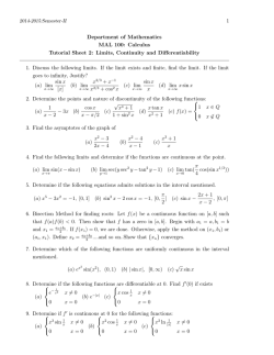

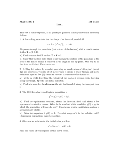
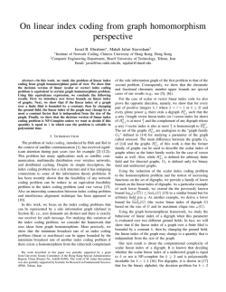


© Copyright 2026