1. Healthcare

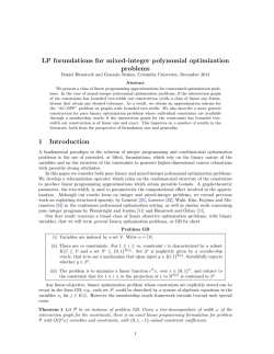
On linear index coding from graph homomorphism
perspective
Javad B. Ebrahimi∗ , Mahdi Jafari Siavoshani†
∗ Institute
† Computer
of Network Coding, Chinese University of Hong Kong, Hong Kong
Engineering Department, Sharif University of Technology, Tehran, Iran
Email: [email protected], [email protected]
Abstract—In this work, we study the problem of linear index
coding from graph homomorphism point of view. We show that
the decision version of linear (scalar or vector) index coding
problem is equivalent to certain graph homomorphism problem.
Using this equivalence expression, we conclude the following
results. First we introduce new lower bounds on linear index
of graphs. Next, we show that if the linear index of a graph
over a finite filed is bounded by a constant, then by changing
the ground field, the linear index of the graph may change by at
most a constant factor that is independent from the size of the
graph. Finally, we show that the decision version of linear index
coding problem is NP-Complete unless we want to decide if this
quantity is equal to 1 in which case the problem is solvable in
polynomial time.
I. I NTRODUCTION
The problem of index coding, introduced by Birk and Kol in
the context of satellite communication [1], has received significant attention during past years (see for example [2]–[12]).
This problem has many applications such as satellite communication, multimedia distribution over wireless networks,
and distributed caching. Despite its simple description, the
index coding problem has a rich structure and it has intriguing
connections to some of the information theory problems. It
has been recently shown that the feasibility of any network
coding problem can be reduce to an equivalent feasibility
problem in the index coding problem (and vice versa) [13].
Also an interesting connection between index coding problem
and interference alignment technique has been appeared in
[10].
In this work, we focus on the index coding problems that
can be represented by a side information graph (defined in
Section II), i.e., user demands are distinct and there is exactly
one receiver for each message. For studying this variation of
the index coding problem, we consider the framework that
uses ideas from graph homomorphism. More precisely, we
show that the minimum broadcast rate of an index coding
problem (linear or non-linear) can be upper bounded by the
minimum broadcast rate of another index coding problem if
there exists a homomorphism from the (directed) complement
The work described in this paper was partially supported by a grant
from University Grants Committee of the Hong Kong Special Administrative
Region, China (Project No. AoE/E-02/08). The work of M. Jafari Siavoshani
was also partially supported by Institute for Research in Fundamental Sciences
(IPM), Tehran, Iran.
of the side information graph of the first problem to that of the
second problem. Consequently, we show that the chromatic
and fractional chromatic number upper bounds are special
cases of our results (e.g., see [5], [6]).
For the case of scalar or vector linear index code we also
prove the opposite direction, namely, we show that for every
pair of positive integers k, l where k = l = 1 or k ≥ 2l and
q
every prime power q, there exits a digraph Hk,l
such that the
q-arry l-length vector linear index (or l-vector index for short)
q
of Hk,l
is at most kl and the complement of any digraph whose
q
q-arry l-vector index is also at most kl is homomorph to Hk,l
.
q
The set of the graphs Hk,l are analogous to the “graph family
Gk ” defined in [14] for studying a parameter of the graph
called minrank. The main difference between the graphs Gk
q
of [14] and the graphs Hk,l
of this work is that the former
family of graphs can be used to describe the scalar index of
graphs where as the latter family works for the case of vector
q
index as well. Also, while Hk,l
is defined for arbitrary finite
field and for directed graphs, Gk is defined only for binary
field and undirected graphs.
Using the reduction of the scalar index coding problem
to the homomorphism problem and the notion of increasing
functions on the set of digraphs, we provide a family of lower
bounds on the linear index of digraphs. As a particular example
of such lower bounds, we extend the the previously known
bound log2 (χ(G)) ≤ lind2 (G) [15] to a similar bound but for
arbitrary field size q. As another example, we derive a lower
−−→
bound for lindq (G) (the vector linear index of digraph G)
based on the size of G and its maximum clique size ω(G).
Using the graph homomorphism framework, we study the
behaviour of linear index of a digraph when this parameter
is evaluated over two different ground fields. In fact, we will
show that if the linear index of a graph over a finite filed is
bounded by a constant k, then by changing the ground field,
the linear index of the graph may change to a quantity that is
independent from the size of the graph.
Our next result is about the computational complexity of
scalar linear index of a digraph. It is known that deciding
whether the scalar linear index of a undirected graph is equal
to k or not is NP-complete for k ≥ 3 and is polynomially
decidable for k = 1, 2 [16]. For digraphs, it is shown in [17]
that for the binary alphabet, the decision problem for k = 2
is NP-complete. We use graph homomorphism framework to
extend this result to arbitrary alphabet.
The remainder of this paper is organised as follows. In
Section II we introduce notation, some preliminary concepts
about graph homomorphism and give the problem statement.
The main results of this paper and their proofs are presented
in Section III and Section IV. In Section V, some applications
of our main results are stated.
transitive. Moreover, if G 4 H and H 4 G, then the digraphs
G and H are homomorphically equivalent (i.e., G → H and
H → G). In this case we write G ∼ H.
II. N OTATION AND P ROBLEM S TATEMENT
Definition 3. Let D ⊆ G be an arbitrary set of digraphs. A
mapping h : D 7→ R is called increasing over D if for every
G, H ∈ D such that G 4 H then h(G) ≤ h(H).
A. Notation and Preliminaries
For convenience, we use [m : n] to denote for the set
of natural numbers {m, . . . , n}. Let x1 , . . . , xn be a set of
variables. Then for any subset A ⊆ [1 : n] we define
xA , (xi : i ∈ A).
All of the vectors are column vectors unless otherwise
stated. If A is a matrix, we use [A]j to denote its jth column.
We use ei ∈ Fkq to denote for a vector which has one at ith
position and zero elsewhere.
A directed graph (digraph) G is represented by G(V, E)
where V is the set of vertices and E ⊆ (V × V ) is the set
+
of edges. For v ∈ V (G) we denote by NG
(v) as the set of
+
outgoing neighbours of v, i.e., NG (v) = {u ∈ V : (v, u) ∈
E(G)}. For a digraph G we use G to denote for its directional
complement, i.e., (u, v) ∈ E(G) iff (u, v) ∈
/ E(G).
A vertex coloring (coloring for short) of a graph (digraph) G
is an assignment of colors to the vertices of G such that there
is no edge between the vertices of the same color. A coloring
that uses k colors is called a k-coloring. The minimum k such
that a k-coloring exists for G is called the chromatic number.
The clique number of a graph (digraph) is defined as the
maximum size of a subset of the vertices such that each
element of the subset is connected to every other vertex in the
subset by an edge (directed edge). Notice that for the directed
case, between any two vertices of the subset there must be
two edges in opposite directions.
The independence number of a graph G, is the size of the
largest independent set1 and is denoted by α(G). For both
directed and undirected graphs, it holds that α(G) = ω(G).
Definition 1 (Homomorphism, see [18]). Let G and H be
any two digraphs. A homomorphism from G to H, written
as φ : G 7→ H is a mapping φ : V (G) 7→ V (H) such that
(φ(u), φ(v)) ∈ E(H) whenever (u, v) ∈ E(G). If there exists
a homomorphism of G to H we write G → H, and if there
is no such homomorphism we shall write G 9 H. In the
former case we say that G is homomorphic to H. We write
Hom(G, H) to denote for the set of all homomorphism from
G to H.
Definition 2. On the set of all loop-less digraphs G, we define
the partial pre order “4” as follows. For every pair of G, H ∈
G, G 4 H if and only if there exists a homomorphism φ :
G 7→ H. It is straightforward to see that “4” is reflexive and
1 An
independent set of a graph G is a subset of the vertices such that no
two vertices in the subset represent an edge of G.
Notice that homomorphically equivalence does not imply
isomorphism between graphs (digraphs). For example, all the
bipartite graphs are homomorphically equivalent to K2 and
therefore are homomorphically equivalent to each other but
they are not necessarily isomorphic.
B. Problem Statement
Consider the communication problem where a transmitter
aims to communicate a set of m messages x1 , . . . , xm ∈ X to
m receivers by broadcasting k symbols y1 , . . . , yk ∈ Y, over a
public noiseless channel. We assume that for each j ∈ [1 : m],
the jth receiver has access to the side information xAj , i.e.,
a subset Aj ⊆ [1 : m] \ {j} of messages. Each receiver j
intends to recover xj from (y1 , . . . , yk , xAj ).
This problem, which is the classical setting of the index coding problem, can be represented by a directed side
information graph G(V, E) where V represents the set of
receivers/messages and there is an edge from node vi to vj ,
i.e., (vi , vj ) ∈ E, if the ith receiver has xj as side information.
An index coding problem, as defined above, is completely
characterized by the side information sets Aj .
In the following definitions, we formally define validity of
an index codes and some other basic concepts in index coding
(see also [2], [5], and [11]).
Definition 4 (Valid Index Code). A valid index code for G
over an alphabet X is a set (Φ, {Ψi }m
i=1 ) consisting of:
(i) an encoding function Φ : X m 7→ Y k which maps m source
messages to a transmitted sequence of length k of symbols
from Y;
(ii) a set of m decoding functions Ψi such that for each i ∈
[1 : m] we have Ψi (Φ(x1 , . . . , xm ), xAi ) = xi .
Definition 5. Let G be a digraph, and X and Y are the source
and the message alphabet, respectively.
(i) The “broadcast rate” of an index code (Φ, {Ψi }) is defined
as
k log |Y|
.
indX (G, Φ, {Ψi }) ,
log |X |
(ii) The “index” of G over X , denoted by indX (G) is defined
as
indX (G) = inf indX (G, Φ, {Ψi }).
Φ,{Ψi }
(iii) If X = Y = Fq (the q-element finite field for some prime
power q), the “scalar linear index” of G, denoted by lindq (G)
is defined as
lindq (G) , inf indFq (G, Φ, {Ψi })
Φ,{Ψi }
in which the infimum is taken over the coding functions of the
form Φ = (Φ1 , . . . , Φk ) and each Φi is a linear combination
φ
G
H
φ−1 (w2 )
φ−1
G
H
Fig. 1. Homomorphism φ maps the vertices of G to the vertices of H. The
pre-image φ−1 of the homomorphism can be considered as a mapping from
V (H) to V (G), i.e., for every w ∈ V (H), φ−1 (w) is the set of all the
vertices v in V (G) such that φ(v) = w.
of xj ’s with coefficients from Fq .
(iv) If X = Flq and Y = Fq , the vector linear index for G,
−−→
denoted by lindq,l (G) is defined as
−−→
lindq,l (G) , inf indFlq (G, Φ, {Ψi })
Φ,{Ψi }
where the infimum is taken over all coding functions Φ =
(Φ1 , . . . , Φk ) such that Φi : Flm
7→ Fq are Fq -linear
q
functions.
(v) The “minimum broadcast rate” of the index coding problem
of G is defined as
ind(G) , inf
X
inf indX (G, Φ, {Ψi }).
Φ,{Ψi }
III. I NDEX C ODING VIA G RAPH H OMOMORPHISM
In this section, we will explain a method for designing index
codes from another instance of index coding problem when
there exists a homomorphism from the complement of the side
information graph of the first problem to that of the second
one. As an application to this result, we will show in Section V
that some of the previously known results about index code
design are special types of our general method.
Theorem 1. Consider two instances of the index coding
problems over digraphs G and H with the source alphabet
X . If G 4 H then
indX (G) ≤ indX (H).
In other words, the function indX (·) is a non-decreasing
function on the pre order set (G, 4).
First we explain the proof idea of Theorem 1 which is as
follows. If G 4 H, by definition there exists a homomorphism
φ : G 7→ H. Notice that the function φ maps the vertices of G
to the vertices of H. Thus we can also consider, φ as a function
from V (G) to V (H). For every vertex w ∈ V (H), we denote
by φ−1 (w) to be the set of all the vertices v ∈ V (G) such that
φ(v) = w; (see Figure 1). This way, we partition the vertices
of G into the classes of the form φ−1 (w) where w ∈ V (H).
Next, we take an optimal index code for H over the source
alphabet X that achieves the rate indX (H). Then, we show
that we can treat every part φ−1 (w) as a single node and
translate the index code of H to one for G. This shows the
statement of the theorem, i.e., indX (G) ≤ indX (H).
Before we formally define the translation and verify its
validity, we will state two technical lemmas that will be
required later in the proof of Theorem 1.
w2
φ−1
⇐=
φ−1 (w1 )
w1
Fig. 2. Demonstration of Lemma 1. Part (i) states that inside each bundle
φ−1 (wi ) we have a clique and part (ii) states that if w2 is an outgoing
neighbour of w1 in H then all of the vertices in φ−1 (w1 ) of G are connected
to all of the vertices in φ−1 (w2 ) of G (note that all of the edges from
φ−1 (w1 ) to φ−1 (w2 ) are not shown in the figure).
Lemma 1. (i) For every w ∈ V (H), φ−1 (w) is a clique in
G.
+
(ii) If w2 ∈ NH
(w1 ), v1 ∈ φ−1 (w1 ), and v2 ∈ φ−1 (w2 ) then
+
v2 ∈ NG (v1 ). (Also see Figure 2).
Proof. (i) If φ−1 (w) is not a clique then ∃v1 , v2 ∈ φ−1 (w)
such that (v1 , v2 ) ∈
/ E(G). Thus (v1 , v2 ) ∈ E(G) implies
that (φ(v1 ), φ(v2 )) = (w, w) should be an edge of H, as
φ : G 7→ H is a homomorphism. But this is a contradiction
since H has no loop.
+
+
(ii) If v2 ∈
/ NG
(v1 ) then v2 ∈ NG
(v1 ) which implies that
+
+
φ(v2 ) ∈ NH (φ(v1 )) and hence w2 ∈ NH
(w1 ). Therefore,
+
w2 ∈
/ NH (w1 ) which is a contradiction.
Definition 6. For every finite set X and positive integer m,
a function f : X m 7→ X is called coordinate-wise one-to-one
if by setting the values for every m − 1 variables of f , it is a
one-to-one function of the remaining variable, i.e., for every
j ∈ [1 : m] and any choice of a1 , . . . , aj−1 , aj+1 , . . . , am ∈
X , the function f (a1 , . . . , aj−1 , x, aj+1 , . . . , am ) : X 7→ X is
one-to-one.
Lemma 2. For every finite set X and m ∈ N, there exists a
coordinate-wise one-to-one function.
Proof. Suppose that |X | = n. Let γ : X 7→ Zn be a bijection
m
between X and integer numbers
Pm modulo n. Define g : X 7→
−1
X by g(x1 , . . . , xm ) , γ ( i=1 γ(xi )). It is straightforward
to check that f is coordinate-wise one-to-one.
Proof of Theorem 1. Suppose that V (H) = {w1 , . . . , wn }
where n = |V (H)|. Let φ : G 7→ H be a homomorphism. As
stated in Lemma 1, the vertex set of G can be partitioned into
n cliques of the form φ−1 (wi ). So, we can list the vertices of
G as V (G) = {v1,1 , . . . , v1,k1 , . . . , vn,1 , . . . , vn,kn } such that
−1
φ−1 (wi ) = {vi,1
P, n. . . , vi,ki } and ki = |φ (wi )|. Note that
m = |V (G)| = i=1 ki .
Let k = indX (H) and ΦH (x1 , . . . , xn ) : X n 7→ Y k (in
addition to a set of decoders {ΨH
i }) be an optimal valid index
code for H over the source alphabet X (and the message
alphabet Y) where xi is the variable associated to the node
wi .
Validity of the index code implies that for every node wi ∈
+
k
|NH
(wi )|
H, there exists a decoding function ΨH
7→
i : Y ×X
X such that
H
ΨH
i (Φ (x1 , . . . , xn ), xN + (wi ) ) = xi
(1)
H
for every choice of (x1 , . . . , xn ) ∈ X n .
Now, we construct a valid index code for G over the same
alphabet sets and the same transmission length k; thus it results
in an index code for G with the same broadcast rate.
Suppose that the variable associated to the node vi,j ∈
V (G) is xi,j ∈ X . First, we construct an instance of index
coding problem over H as follows. Then using Lemma 2, we
pick n coordinate-wise one-to-one function gi : X ki 7→ X
and set xi = gi (xi,1 , . . . , xi,kiP
). Now, we define the index
code encoder function ΦG : X ( ki ) 7→ Y k as follows:
ΦG (x1,1 , . . . , x1,k1 , . . . , xn,1 , . . . , xn,kn ) ,
ΦH (g1 (x1,1 , . . . , x1,k1 ), . . . , gn (xn,1 , . . . , xn,kn )) .
To complete the proof, we need to construct the decoding
functions for all the receivers vi,j . Due to the symmetry, we
only construct the decoding function for v1,1 .
+
First define the function h : Y k × X |NG (v1,1 )| 7→ X as
follows
h(y1 , . . . , yk , xN + (v1,1 ) ) = ΨH
1 (y1 , . . . , yk , xN + (w1 ) ).
G
H
Note that h is a well defined function since if xN + (v1,1 ) is
G
given as parameter of h, xN + (w1 ) is also known. This is due
H
+
+
to the fact that for every wi ∈ NH
(w1 ), φ−1 (wi ) ⊆ NG
(v1,1 )
by Lemma 1 and xi = gi (xi,1 , . . . , xi,ki ) is known to wi .
Notice that for the defined function h we have
h ΦG (x1,1 , x1,2 , . . . , xn,kn ), xN + (v1,1 )
G
H
H
= Ψ1 Φ g1 (x1,1 , . . . , x1,k1 ),
. . . , gn (xn,1 , . . . , xn,kn ) , xN + (w1 )
H
= g1 (x1,1 , . . . , x1,k1 )
where the first equality is by the definition of h and the second
equality is by (1).
Note that by part (i) of Lemma 1, we know that
x1,2 , . . . , x1,k1 are among the out neighbours of v1,1 , i.e.,
x1,i ∈ xN + (v1,1 ) for i ∈ [2 : k1 ]. Define the function
G
g1,1 : X 7→ X as g1,1 (x) , g1 (x, x1,2 , x1,3 , . . . , x1,k1 ).
Therefore
(g1,1 )−1 h(ΦG (x1,1 , . . . , xn,kn ), xN + (v1,1 ) ) =
G
(g1,1 )−1 (g1 (x1,1 , . . . , x1,k1 )) = x1,1 .
Hence, we can define the decoding function
ΨG
1,1
as
ΨG
1,1 y1 , . . . , yk , xN + (v1,1 ) ,
This shows the validity of the proposed index code for the
problem defined over G and so completes the proof.
As a consequence of Theorem 1 we have the following
corollary.
Corollary 1. Consider two instances of the index coding
problems over the digraphs G and H. If G 4 H then we
have
1) for general multi-letter index codes: ind(G) ≤ ind(H),
−−→
−−→
2) for linear vector index codes: lindq,l (G) ≤ lindq,l (H),
3) for linear scalar index codes: lindq (G) ≤ lindq (H).
Proof. In the inequality of Theorem 1, if we take the infimum
of both sides, we derive Part 1. To prove the other parts of the
corollary, notice that in both cases of scalar and vector index
code, we can define the function g in the proof of Theorem 1 to
be the sum function and therefore, it is a linear function. Hence
the functions ΦG and ΨG
i,j are also linear. This completes the
proof.
IV. A N E QUIVALENT F ORMULATION FOR L INEAR I NDEX
C ODING P ROBLEM
q
For k ≥ l ∈ Z+ , let Gk,l
be the set of all the finite digraphs
−−→
q
G for which lindq,l (G) ≤ kl . Although Gk,l
is an infinite
q
family of digraphs, in this section, we will show that Gk,l
has a maximal member with respect to the pre order “4”. We
q
give an explicit construction for a maximal element of Gk,l
q
which we call it Hk,l .
First, let us state the following definition.
Definition 7. A family of graphs {Gk }∞
k=1 is called (q, l)index code defining ((q, l)-ICD) if and only if for every (side
information) digraph G we have
−−→
k
lindq,l (G) ≤ ⇐⇒ G 4 Gk .
l
It is easy to see that if {Gk }∞
k=1 is a (q, l)-ICD, so is
0
the family {G0k }∞
k=1 where Gk and Gk are homomorphi∞
cally equivalent. In particular, if {Gk }k=1 is a (q, l)-ICD
in which no Gk can be replaced with a smaller digraph,
then Gk ’s are cores and conversely, if {Gk }∞
k=1 is a (q, l)ICD, {Core(Gk )}∞
k=1 is the unique smallest (q, l)-ICD, up to
isomorphism2 .
q
Construction 1 (Graph Hk,l
). For every positive integers
k ≥ l and prime power q, let V be the set of all full rank
matrices in Fk×l
q . We define the set W to be
W = (v, w) | v, w ∈ V, and v> w = Il
where Il is an l × l identity matrix.
q
Now, we construct graph Hk,l
as follows. The vertex
q
q
set of Hk,l is V (Hk,l ) = W and (v, w), (v0 , w0 ) ∈
q
E(Hk,l
) if and only if v> w0 6= 0l . In other
G
(g1,1 )−1 ◦ h y1 , . . . , yk , xN + (v1,1 ) .
G
2 For
the definition of core of a graph, see [18, Chapter 1.6].
(a2 , a3 ) w3
(a2 , a2 )
w2
w4
(a3 , a2 )
(a1 , a3 )
w1
w5
w6
(a1 , a1 )
(a3 , a1 )
Fig. 3. The digraph H22 consists of 6 vertices. The graph vertices are labelled
by pair of vectors (matrices) where each element is one of the following
vectors a1 = [0 1]> , a2 = [1 0]> , and a3 = [1 1]> .
q
words, (v, w), (v0 , w0 ) ∈ E(Hk,l
) if and only if
0
0
> 0
(v, w), (v , w ) ∈ W and v w = 0l . This construction
leads to a graph of size
q
|V (Hk,l
)| = q l(k−l)
l−1
Y
Let us group the columns of A into submatrices Ei ∈ Fk×l
q
where each Ei is the encoding coefficients associated to
the source symbols x1i , . . . , xli , i.e., A = [ E1 · · · Em ].
Notice that Ej can be viewed as the contribution of the
source symbols x1j , . . . , xlj in the set of transmitted messages;
therefore, rank(Ej ) = l (consequently, none of the columns
of Ej are zero). Otherwise, there does not exist enough linear
combinations of x1j , . . . , xlj in the transmitted messages and
hence the jth receiver cannot recover its demand. Now for
the vertex vj ∈ V (G) corresponding to the jth message
(i.e., source symbols x1j , . . . , xlj ), define the encoding matrix
E(vj ) , Ej .
Let vi be an arbitrary node of G. We know that
>
{a>
1 x, . . . , ak x} together with the side information of vi
can be used in order to recover x1i , . . . , xli . This means that
there exist l linear combinations of the transmitted messages
which is sufficient for the ith receiver to recover its demand
x1i , . . . , xli . Let us assume that these linear combinations are
of the following form
D>
i Ax =
(q k − q i ).
m
X
D>
i Ej xj
j=1
i=0
q
For convenience we drop the index l from Hk,l
when l = 1
(i.e., for the case of scalar linear index code).
Example 1. As an example, let us consider H22 . Here we have
V = {e1 , e2 , e1 + e2 }. So it can be easily observed that H22
has 6 nodes as follows
V (H22 ) = (e1 , e1 ), (e1 , e1 + e2 ), (e2 , e2 )
(e2 , e1 + e2 ), (e1 + e2 , e1 ), (e1 + e2 , e2 ) .
The graph
H22
2
Now, we have the following result.
where A ∈
− a>
k −
xlm




S(vi ) = 
.. 
. 
3
Theorem 2. For every prime power q and positive integer l,
q ∞
the family {Hk,l
}k=l introduced above, is (q, l)-ICD.
−−→
Proof. We need to show that ∀G : lindq,l (G) ≤ k/l ⇔ G 4
q
Hk,l .
−−→
First, to prove the direct part, suppose that lindq,l (G) ≤ k/l.
So we know that there exists an index code of transmitted
sequence length k for this problem. We also know that each
transmitted message yj , j ∈ [1 : k], is a linear combination
of the source symbols x = [x11 , . . . , xl1 , . . . , x1m , . . . , xlm ]> ∈
1
l >
Flm
q where xi = [xi , . . . , xi ] is the source symbols assigned
to the ith message and m = |V (G)|. Let aj ∈ Flm
be the
q
coefficient of the jth transmitted message. Hence, the set of
messages transmitted by the source is equal to

  1 


x1
− a>
y1
1 −



 .. 
. 
.
..
 ×  .. 
 .  = Ax = 
Fk×lm
.
q
vj1
1
is depicted in Figure 3.
yk
where Di ∈ Fk×l
q .
Clearly rank(Di ) = l, since xji ’s are independent from each
other and also because by using its side information alone,
vi cannot recover xji ’s. Define the decoding matrix D(vi )
assigned to vi to be D(vi ) , Di .
+
Let r = |NG
(vi )| and S(vi ) ∈ Flr×lm
be the side informaq
tion matrix of the ith receiver where S(vi )x determines the
side information that vi has. Without loss of generality we can
assume that S(vi ) is a block matrix of the following form
r
···
···
···
..
.
···
vj2
vjr
Il
0l
0l
..
.
···
···
···
..
.
0l
Il
0l
..
.
···
···
···
..
.
0l
0l
0l
..
.
···
···
···
..
.
0l
···
0l
···
Il
···







+
NG
(vi )
where vj1 , . . . , vjr ∈
and each block is an l × l matrix
that is either 0l or Il .
Decodability of D(vi ) means that the node vi can recover
x1i , . . . , xli from D(vi )> Ax and its side information S(vi )x.
In other words, in the matrix D(vi )> A, all the non-zero blocks
should be known by vi (through its side information) except
the ith block (i.e., the block D(vi )> E(vi )) where the ith block
is also non-zero. Now, by considering the row reduced echelon
form of matrix
D(vi )> A
,
S(vi )
it can be observed that we should have
rank D(vi )> Ei (vi ) = l
(2)
and for i 6= j we should have
D(vi )> E(vj ) 6= 0l =⇒ (vi , vj ) ∈ E(G)
(3)
or equivalently,
(vi , vj ) ∈
/ E(G) =⇒ D(vi )> E(vj ) = 0l .
(4)
Note that if D(vi ) is right multiplied by a full rank matrices
the conditions (2)-(4) are not changed. Hence it is possible to
further restrict (2) while keeping the decodability of D(vi ). It
means that without loss of generality, the condition (2) can be
replaced by
(5)
D(vi )> Ei (vi ) = Il .
Secondly, to complete the proof of the direct part of the
q
theorem, we present a function φ : V (G) 7→ V (Hk,l
) and
show that φ is a homomorphism.
For
each
v
∈
V
(G)
i
define φ(vi ) = D(vi ), E(vi ) . By (5), if vi ∈ V (G) clearly
q
).
D(vi )> E(vi ) = Il . Hence, φ(vi ) ∈ V (Hk,l
Then we need to show that φ preserves the edges. Suppose
that (vi , vj ) ∈ E(G). So we have (vi , vj ) ∈
/ E(G) and by (4)
q
D(vi )> E(vj ) = 0. Now by construction of Hk,l
, this implies
that
q
D(vi ), E(vi ) , D(vj ), E(vj ) ∈ E(Hk,l
),
q
namely, φ(vi ), φ(vj ) ∈ E(Hk,l
). This shows that φ is a
q
homomorphism from G to Hk,l . So the direct part of the
theorem is proved.
−−→
So far, we have proved that if lindq,l (G) ≤ k/l then
q
G 4 Hk,l
. Now, we show the reverse part; namely, we show
−−→
q
q
that G 4 Hk,l
implies lindq,l (G) ≤ k/l. If G 4 Hk,l
, by
q
q
definition, we have G → Hk,l . Suppose that φ : G → Hk,l
is a homomorphism. For each vi ∈ V (G) let φ(vi ) =
q
). Hence, Dφ (vi ) and Eφ (vi )
(Dφ (vi ), Eφ (vi )) ∈ V (Hk,l
k×l
are full rank matrices in Fq . Since φ is a homomorphism,
(vi , vj ) ∈ E(G) ⇒ Dφ (vi )> Eφ (vj ) = 0. Equivalently,
Dφ (vi )> Eφ (vj ) 6= 0 ⇒ (vi , vj ) ∈ E(G). Therefore, it is
easy to see that the index coding defined by the k × lm matrix
A = Eφ (v1 ) · · · Eφ (vm )
is a valid index code of transmitted sequence length k over
Fq for G. Furthermore, the decoding algorithm for each node
vi ∈ V (G) is to take the linear combination of the transmitted
messages (rows of A) with coefficients from Dφ (vi ). Now
−−→
by Definition 5, we have lindq,l (G) ≤ k/l. This complete the
proof of the theorem.
q
A. Properties of graph Hk,l
In this section, we state some properties of the graph family
q ∞
{Hk,l
}k=1 where are used in the subsequent sections.
Lemma 3. For every k
lindq (Hkq ) = k.
∈ Z+ and prime power q,
Proof. Since the identity function from Hkq to itself is a
homomorphism, therefore Hkq 4 Hkq and by Theorem 2,
we have lindq (Hkq ) ≤ k. Now, if lindq (Hkq ) 6= k, then
lindq (Hkq ) ≤ k − 1. Let G be the graph with k vertices but no
edge. Clearly lindq (G) = k. By Theorem 2 we have G 4 Hkq
and by Theorem 1 we have
k = lindq (G) ≤ lindq (Hkq ) ≤ k − 1
which is a contradiction.
Lemma 4. For every k ≥ l ∈ Z+ and prime power q, graph
q
Hk,l
is vertex-transitive3 .
Proof. From the definition of vertex transitivity, it is enough
q
to show that for every arbitrary vertex (d, e) ∈ V (Hk,l
),
q
there exists an automorphism φ ∈ Aut(Hk,l ) such that
φ(d, e) = (B, B) where B = [ Il 0l×(k−l) ]> ∈ Fk×l
q .
Let {ξ 1 , . . . , ξ k−l } be a basis for the orthogonal complement
q
of column space of e, i.e., ξ >
i e = 0. Since (d, e) ∈ V (Hk,l )
>
therefore d e = I and hence [d]j ∈
/ Span(ξ 1 , . . . , ξ k−l ).
Thus, {ξ 1 , . . . , ξ k−l , [d]1 , . . . , [d]l } form a basis for Fkq . Define the k × k invertible matrix
X = [d ξ 1 · · · ξ k−l ]> .
Notice that X−> d = B since X> B = d. Also, notice
that X · e = B since d> e = Il . Define the function
q
q
φ : V (Hk,l
) 7→ V (Hk,l
) as φ(u, v) = X−> u, Xv . Since
−>
>
(X u) Xv = Il , we conclude that φ(u, v) is indeed an
q
element of V (Hk,l
). Last, we need to show that for each edge
0
0
(u, v), (u , v ) , the image under φ is also an edge (more
precisely, we need to show
edges and non that φ preserves
q
then u> v0 6= 0.
edges). If (u, v), (u0 , v0 ) is an edge in Hk,l
Thus, (X−> u)> Xv0 6= 0 and therefore φ(u, v), φ(u0 , v0 ) is
an edge. By applying the same argument it can be shown that
φ also preserves non-edges and this completes the proof.
Obviously, as a result of Lemma 4, we have the following
corollary.
q
Corollary 2. Graph Hk,l
is also vertex transitive.
In the following, we obtain an upper bound on the chromatic
q
number of Hk,l
. But before that let us state the following
definition.
Definition 8. A non-zero vector a ∈ Fkq is called normal if its
first non-zero element is equal to 1, i.e.,
a = (0, . . . , 0, 1, ?, . . . , ?)> .
with non-zero columns is called normal
A matrix A ∈ Fk×r
q
if all of its columns are normal.
For a matrix A, we define Υ(A) to be the normalization of
A, namely, the operator Υ(·) normalizes every column of A
by multiplying it with a (non-zero) constant. In other words,
we can write Υ(A) = A · Λ where Λ ∈ Fr×r
is a diagonal
q
matrix with non-zero elements on its diagonal.
3 A graph H is said to be vertex-transitive if for any vertices u, v of H
some automorphism of H (i.e., a bijective homomorphism of H to H) takes
u to v (e.g., see [18, Chapter 1, p.14]).
q
Lemma 5. The chromatic number of Hk,l
can be upper
bounded as
Ql−1 k
(q − q i )
q
.
χ(Hk,l ) ≤ i=0
(q − 1)l
Proof. To proof the assertion
Ql−1of lemma, we show that qthere
exists a colouring of size i=0 (q k − q i )/(q − 1)l for Hk,l
. In
fact we show that if d ∈ V is the decoding matrix assigned to a
q
vertex of Hk,l
then Υ(d) assigned to that vertex is a candidate
for such a colouring
(see Construction 1). First, notice that
Ql−1
there are at most i=0 (q k − q i )/(q − 1)l of such matrices
(colours). Then we need to show that this assignment leads to
q
. To this end, consider two vertices
a proper colouring of Hk,l
q
(d, e), (d0 , e0 ) ∈ V (Hk,l
) which have the same colour, i.e.,
we have Υ(d) = Υ(d0 ). From Construction 1, we know that
d> e = I and d0> e0 = I. Because Υ(d) = Υ(d0 ) we can write
d = N · Λ1 and d0 = N · Λ2 where N is a normal matrix.
Now we can write
> 0
> 0
d e = (N · Λ1 ) e
= Λ1 N> e0
= Λ1 Λ−1
2
6= 0
which, by using Construction 1, it means that there is no edge
q
in Hk,l
from (d, e) to (d0 , e0 ). A similar argument shows
that there is no edge in the reverse direction as well. So this
completes the proof of lemma.
q
Lemma 6. The clique number of Hk,l
is lower bounded as
follows
q
q
ω(Hk,l
) = α(Hk,l
) ≥ q l(k−l)
l−1
Y
(q l − q i ).
i=0
Proof. Consider a set C of pairs of matrices defined as follows
(
−> J
J
C = (a, b) a =
, b=
,
T
0
)
(k−l)×l
J ∈ Fl×l
.
q , rank(J) = l, T ∈ Fq
Notice that for each pair of matrices (a, b) ∈ C we have
a> b = J−1 J = Il for some full rank matrix J. This shows
q
that C ⊂ V (Hk,l
).
q
Now, it remains to show that C forms a clique in Hk,l
. Let
0
0
(a, b), (a , b ) ∈ C be two arbitrary vertices in C. Then we
can write
a> b0 = J−1 J0
6= 0
since J and J0 are full rank. By using Construction 1, it means
q
that there is an edge from (a, b) to (a0 , b0 ) in Hk,l
. Similarly,
0
it can be shown that there is an edge from (a , b0 ) to (a, b)
q
in Hk,l
. This concludes the Lemma.
V. A PPLICATIONS
In this section, we demonstrate several applications of the
results stated in the previous sections.
A. Upper Bounds
Here, we will show that some of the earlier upper bounds
are only special cases of Corollary 1.
Example 2. One of the earliest upper bounds on the lind2 (G)
is χ(G) where χ(·) is the chromatic number of a graph
(e.g., see [19]). Notice that in our framework, this result
is an immediate consequence of Corollary 1, Part 3. That
is, if χ(G) = r then G → Kr where Kr is a complete
graph with r vertices (e.g., see [18, Chapter 6, p.204]. Thus,
lindq (G) ≤ lindq (Kr ) = r = χ(G). Notice that using our
method, as shown above, the colouring upper bound naturally
extends for every prime power q.
In Example 3, using graph homomorphism framework, we
derive the fractional chromatic number upper bound on the
length of index code [5]. To this end, let us first state the
definition of Kneser graphs.
Definition 9 (Kneser graphs K(n, l)). Given two positive
integers l ≤ n, the Kneser graph K(n, l) is the graph whose
vertices represent the l-subsets of [1 : n] and two vertices are
connected if and only if they correspond to disjoint subsets.
Example 3. In [5], it is shown that ind(G) ≤ χf (G)
where χf (·) is the fractional chromatic number of a graph.
However, using the graph homomorphism framework, this
result follows immediately from Corollary 1, Part 2, and the
fact that if χf (G) = nl then G → K(n0 , l0 ) for some pair
0
of integers n0 , l0 with nl = nl0 (see [18, Theorem 6.23]).
(a)
−−→
−−→
Thus, lindq,l (G) ≤ lindq,l (K(n, l)) ≤ nl = χf (G) where
the inequality (a) follows from Lemma 7.
Lemma 7. For the vector linear index code of a complement
of Kneser graph K(n, l), we have
−−→
n
lindq,l (K(n, l)) ≤ .
l
Proof. We know that χf (K(n, l)) = nl (e.g., see [18], Theorem 6.23 and Proposition 6.27). Thus, a natural fractional
colouring for K(n, l) is to use the l-subsets of [1 : n] assigned
to its vertices. Let Su ⊂ [1 : n] be the set of colours associated
to u ∈ V (K(n, l)).
Now, we will show that the sets of colours Su impose a
vector linear index code for the index coding problem defined
with the side information graph K(n, l). To this end, we assign
l independent source variables to each vertex u ∈ V (K(n, l))
and label them as xui ∈ Fq where i ∈ Su . Then the transmitter
broadcasts the following n messages over the public channel
X
yi =
xui , ∀i ∈ [1 : n].
u: i∈Su
From the definition of Kneser graphs we know that
(u, v) ∈ E(K(n, l)) ⇐⇒ Su ∩ Sv 6= ∅.
As a result, for each i ∈ Su , the receiver u can recover the
variable xui because by construction receiver u is connected
to all nodes v ∈ V (K(n, l)) such that i ∈ Sv and it has all of
the required variables to recover xui .
The above argument presents a scheme which shows that
by sending n symbols over Fq , each receiver node can recover
a vector of source variables of length l over Fq . This proofs
the claim of the lemma.
The crucial observation in the above examples is that the
parameters χ(G) and χf (G) can be defined using existence
of homomorphisms from G to the family of complete graphs
and Kneser graphs, respectively.
Similar to Lemma 3, we can observe that:
Observation 1. For every k ∈ Z+ and prime power q,
−−→
q
lindq,l (Hk,l
) ≤ k/l.
q
is homomorphic to itself then the assertion
Proof. Since Hk,l
follows directly from Theorem 2.
−−→
Notice that if there exists a graph G such that lindq,l (G) =
k/l then Observation 1 holds with equality. This is because if
−−→
lindq,l (G) = k/l then by Theorem 2, G is homomorphic to
−−→
−−→
q
q
Hk,l
and therefore k/l = lindq,l (G) ≤ lindq,l (Hk,l
) ≤ k/l.
Unfortunately, we do not know if such G exists but we make
the following conjecture.
In the following we introduce another tool to find lower
−−→
bounds on lindq,l (G). Hell and Nesetril in [18, Proposition 1.22] showed that if a graph H is vertex transitive and
φ : G → H is a homomorphism, then for every graph K
|H|
|G|
≤ N (H,K)
in which N (L, K) is the size of
we have N (G,K)
the largest induced subgraph L0 of L such that there exists a
homomorphism from L0 to K. Even though this result is stated
for undirected graphs, its proof naturally extends to digraphs.
Therefore, using this result and Theorem 2 we can deduce the
following theorem.
Theorem 4. For every digraph G, if there exists a digraph
Ksuch that
q
|Hk,l
|
|G|
>
q
N (G, K)
N (Hk,l , K)
−−→
then lindq,l (G) > k/l.
Proof. We prove the theorem by contradiction. Suppose
−−→
that lindq,l (G) ≤ k/l. Then by Theorem 2, we have
q
q
) 6= ∅. Also by Corollary 2, Hk,l
is a vertex
Hom(G, Hk,l
transitive digraph. Now we can apply the result of [18,
Proposition 1.22] to qconclude that for every digraph K we
|Hk,l |
|G|
have N (G,K)
≤
which is a contradiction. Thus we
q
N (Hk,l ,K)
are done.
Conjecture 1. For every prime power q and any pair of (k, l),
−−→
k ≥ l of positive integers, lindq,l (K(k, l)) = k/l.
An interesting special case of Theorem 4 is when K is a
complete graph with r vertices. In this case N (G, K) is equal
to the size of the largest r-colourable induced subgraph of G.
In particular the following corollary holds.
B. Lower Bounds
Corollary 3. For every digraph G if
l−1
As a result of Theorem 2, we can prove the following
lemma.
Y qk − qi
|G|
>
ω(G) i=0 q l − q i
Lemma 8. Suppose that h is an increasing function on (G, 4)
q
and r is an upper bound on h(Hk,l
). For every digraph G, if
−−→
h(G) > r then lindq,l (G) > k/l.
−−→
q
Proof. If lindq,l (G) ≤ k/l then by Theorem 2, G 4 Hk,l
and
q
therefore h(G) ≤ h(Hk,l ) ≤ r which is a contradiction.
−−→
then lindq,l (G) > k/l. In other words, we can state the
−−→
following expression to lower bound lindq,l (G),
"l−1
#
l−1
−−→
X
Y
l lindq,l (G)
i
l
i |G|
logq q
− q ≥ logq
.
(q − q )
ω(G)
i=0
i=0
Lemma 8 is a useful tool to find lower bounds on the scalar
linear index of an index coding problem. Actually for every
increasing function h on (G, 4) we have one lower bound
on the index coding problem. In the next theorem, using
Lemma 8, we provide an alternative proof for the known lower
bound on lindq (G) (i.e., for the scalar case when l = 1) in
terms of the chromatic number of G [15].
Theorem 3. For every digraph G we have
lindq (G) ≥ logq (q − 1)χ(G) + 1 .
Proof. The function h(G) = χ(G) is an increasing function on (G, 4) (e.g., see [18, Corollary 1.8]). Suppose that
lindq (G) = k. Therefore, by Theorem 2, we have G 4 Hkq .
k
−1
Thus χ(G) ≤ χ(Hkq ) ≤ qq−1
where the last inequality follows
from Lemma 5. This completes the proof of theorem.
Proof. In Theorem 4 set K to be K1 . Then ω(G) = α(G) =
N (G, K1 ). Now Lemma 6 completes the proof.
For the scalar case where l = 1, we can derive a slightly
stronger lower bound as stated in the following (see [20])
(q 2 − 1)(q − 1) |G|
lindq (G) ≥ logq 1 +
.
4q
ω(G)
Example 4. Let G be a directed graph with n vertices so that
for every pair (i, j) of the vertices either (i, j) ∈ E(G) or
(j, i) ∈ E(G) but not both. In this case, α(G) = ω(G) = 1.
The lower bound derived above translates to
(q 2 − 1)(q − 1)
lindq (G) ≥ logq 1 +
n .
4q
This lower bound is slightly better than the lower bound
obtained from Theorem 3 and is significantly stronger that
the trivial bound lindq (G) ≥ α(G).
(e1 , e1 )
(e2 , e2 )
(e1 + e2 , e2 )
(e2 , e1 − e2 )
Fig. 4. The induced subgraph D of Hkq which is used in the proof of
Theorem 6 to show that the core of Hkq cannot be a directed cycle.
C. Computational Complexity of lindq (·)
By applying the result of [21] that proves the conjecture
[18, Conjecture 5.16] and using Theorem 2, we show that the
decision problem of lindq (G) ≤ k is NP-complete for k ≥ 2.
First, let us state the following theorem.
Theorem 5 (see [21] and [18, Conjecture 5.16]). Suppose that
H is a digraph with no vertex of in degree or out degree one.
If core of H is not a directed cycle then the following decision
problem is NP-complete.
Input:
Output:
A digraph G
If hom(G, H) 6= ∅ then return “yes,” else
return “no.”
We will apply Theorem 5 to digraphs Hkq for every k ≥ 2.
Theorem 6. For every finite field Fq and every k ≥ 2 the
following decision problem is NP-complete.
Input:
Output:
A digraph G
If lindq (G) ≤ k return “yes,” otherwise
return “no.”
Proof. Based on Theorem 2 and Theorem 5, it is sufficient to
show that Hkq has no vertex of in/out degree one and also its
core is not a directed cycle. From Construction 1 we know
that for k ≥ 2, Hkq has no source or sink. It remains to show
that the core of Hkq for any prime power q and any integer k,
is not a directed cycle.
To this end, consider the subgraph D of Hkq depicted in
Figure 4. Clearly from this induced subgraph D there is no
homomorphism to any directed cycle. Thus the core of Hkq
cannot be a directed cycle.
Notice that the NP-completeness of the decision problem
lindq (G) ≤ k was known for q = 2 and k ≥ 3, see [14], [16].
In fact this decision problem is NP-complete even when G is
an undirected graph [16]. However, for undirected graphs, the
decision problem lindq (G) ≤ 2 is polynomially solvable since
for undirected graphs we have lindq (G) ≤ 2 if and only if G
is complement of a bipartite graph. Theorem 6 shows that for
digraphs, even the decision problem lindq (G) ≤ 2 is hard.
D. Index Codes and Change of Field Size
Existence of a certain index code for a given graph over
a fixed finite field is equivalent to the existence of linear
combinations of the source messages over the ground field
with certain Algebraic / Combinatorial constraints. If the
ground field is changed, there is no natural way of updating
the index code over the new field. In other words, if for a fixed
graph G, an index code over a finite field Fq1 is given, there
is no natural way to construct some index code for the same
graph but over a different field Fq2 .
Here we use the results of Theorem 1 and Theorem 2 to
show that if the field size is changed, the corresponding linear
indices can at most differ by a factor that depends only on
the field sizes and is independent from the size of the graph.
More precisely the following result holds:
Theorem 7. Let G be a graph and q1 , q2 are two different
−−→
prime powers. Suppose that lindq1 ,l1 (G) = kl11 . Then,
−−→
−−→
lindq2 ,l2 (G) ≤ lindq2 ,l2 (Hkq11,l1 )
Ql1 −1 k1
(q − q i )
≤ i=0 1 l1 1 .
(q1 − 1)
−−→
Proof. We know that lindq1 ,l1 (G) = kl11 . By Theorem 2,
−−→
G 4 Hkq11,l1 and then by Theorem 1, lindq2 ,l2 (G) ≤
−−→
lindq2 ,l2 (Hkq11,l1 ). The last inequality of the assertion follows
from the colouring upper bound, Example 2, Lemma 5, and
the fact that χf (Hkq11,l1 ) ≤ χ(Hkq11,l1 ).
Remark 1. In fact, for the scalar index coding problem, in
[3], it has been shown that for every pair of finite fields Fp and
Fq of different characteristics and for every 0 < < 1, there
exists a graph G with arbitrarily large number of vertices n
such that lindp (G) < n and lindq (G) > n1− . The previous
theorem shows that in the result of [3], n can not be replaced
by a constant.
ACKNOWLEDGEMENT
The authors would like to thank Dr. P. Hell, Dr. S. Jaggi
and Dr. A. Rafiey for their invaluable comments.
R EFERENCES
[1] Y. Birk and T. Kol, “Informed-source coding-on-demand (iscod) over
broadcast channels,” in in Proc. 17th Ann. IEEE Int. Conf. Comput.
Commun. (INFOCOM), 1998, pp. 1257–1264.
[2] N. Alon, E. Lubetzky, U. Stav, A. Weinstein, and A. Hassidim, “Broadcasting with side information,” in Proceedings of the 2008 49th Annual
IEEE Symposium on Foundations of Computer Science, ser. FOCS ’08,
2008, pp. 823–832.
[3] E. Lubetzky and U. Stav, “Nonlinear index coding outperforming the
linear optimum,” IEEE Trans. Inf. Theory, vol. 55, no. 8, pp. 3544–
3551, 2009.
[4] S. El Rouayheb, A. Sprintson, and C. Georghiades, “On the index coding
problem and its relation to network coding and matroid theory,” IEEE
Trans. Inf. Theory, vol. 56, no. 7, pp. 3187–3195, 2010.
[5] A. Blasiak, R. D. Kleinberg, and E. Lubetzky, “Index coding via linear
programming,” CoRR, vol. abs/1004.1379, 2010.
[6] Z. Bar-Yossef, Y. Birk, T. S. Jayram, and T. Kol, “Index coding with side
information,” IEEE Trans. Inf. Theory, vol. 57, no. 3, pp. 1479–1494,
2011.
[7] Y. Berliner and M. Langberg, “Index coding with outerplanar side
information,” in IEEE Int. Symp. Inf. Theory, 2011, pp. 806–810.
[8] I. Haviv and M. Langberg, “On linear index coding for random graphs,”
in IEEE Int. Symp. Inf. Theory, 2012, pp. 2231–2235.
[9] A. Tehrani, A. Dimakis, and M. Neely, “Bipartite index coding,” in IEEE
Int. Symp. Inf. Theory, 2012, pp. 2246–2250.
[10] H. Maleki, V. R. Cadambe, and S. A. Jafar, “Index coding - an
interference alignment perspective,” CoRR, vol. abs/1205.1483, 2012.
[11] K. Shanmugam, A. G. Dimakis, and M. Langberg, “Local graph coloring
and index coding,” CoRR, vol. abs/1301.5359, 2013.
[12] F. Arbabjolfaei, B. Bandemer, Y.-H. Kim, E. Sasoglu, and L. Wang, “On
the capacity region for index coding,” in IEEE Int. Symp. Inf. Theory,
2013, pp. 962–966.
[13] M. Effros, S. Y. E. Rouayheb, and M. Langberg, “An equivalence
between network coding and index coding,” CoRR, vol. abs/1211.6660,
2012.
[14] E. Chlamtac and I. Haviv, “Linear index coding via semidefinite programming,” CoRR, vol. abs/1107.1958, 2011.
[15] M. Langberg and A. Sprintson, “On the hardness of approximating
the network coding capacity,” in IEEE International Symposium on
Information Theory, 2008, pp. 315–319.
[16] R. Peeters, “Orthogonal representations over finite fields and the chromatic number of graphs,” Combinatorica, vol. 16, no. 3, pp. 417–431,
1996.
[17] S. H. Dau, V. Skachek, and Y. M. Chee, “Optimal index codes with
near-extreme rates,” Information Theory, IEEE Transactions on, vol. 60,
no. 3, pp. 1515–1527, 2014.
[18] P. Hell and J. Nesetril, Graphs and Homomorphisms, ser. Oxford Lecture
Series in Mathematics and Its Applications. OUP Oxford, 2004.
[19] Z. Bar-Yossef, Y. Birk, T. S. Jayram, and T. Kol, “Index coding with side
information,” in Proceedings of the 47th Annual IEEE Symposium on
Foundations of Computer Science, ser. FOCS ’06, 2006, pp. 197–206.
[20] J. Ebrahimi Boroojeni and M. Jafari Siavoshani, “Linear index coding
via graph homomorphism,” in IEEE International Conference on Control, Decision and Information Technologies (CoDIT), 2014.
[21] L. Barto, M. Kozik, and T. Niven, “The csp dichotomy holds for digraphs
with no sources and no sinks (a positive answer to a conjecture of
bang-jensen and hell),” SIAM Journal on Computing, vol. 38, no. 5, pp.
1782–1802, 2009.