
dsPICworks Software
dsPICworksTM Version 1.0
Data Analysis and
Digital Signal Processing Software
User’s Guide
Developed for
Microchip Technology Inc.
by
Momentum Data Systems Inc.
Copyright 1993-2003 Momentum Data Systems, 17330 Brookhurst Street, Suite 230, Fountain
Valley, CA 92708
World rights reserved. No part of this publication may be stored in a retrieval system, transmitted,
or reproduced in any way, including but not limited to photocopy, photograph, magnetic or other
record, without the prior agreement and written permission of Momentum Data Systems.
Information in this manual is subject to change without notice and does not represent a commitment on the part of Momentum Data systems. The software described in this reference guide is
furnished under a license agreement and may be used or copied only in accordance with the terms
of the agreement.
This manual was produced and printed using SnagIt and FrameMaker for Windows.
FrameMaker is a trademark of Adobe Systems Inc. SnagIt is a registered trademark of Techsmith
Corp.
QEDesign is trademarked to Momentum Data Systems Inc.
dsPICworks and dsPIC are trademarks, and MPLAB is a registered trademark, of Microchip
Technology Inc.
All trademarks and copyrights are the property of their respective owners.
LICENSE AGREEMENT
PLEASE READ THE FOLLOWING TERMS AND CONDITIONS
BEFORE USING THIS PROGRAM. USE OF THE PROGRAM INDICATES YOUR ACCEPTANCE OF THESE TERMS AND CONDITIONS. IF YOU DO NOT AGREE WITH THEM, PROMPTLY
RETURN THE UNUSED PROGRAM ALONG WITH PROOF OF PURCHASE AND YOUR MONEY WILL BE REFUNDED BY SELLER
Momentum Data Systems, provides this program and
licenses its use. You assume responsibility for the selection
of the program to achieve your intended results, and for the
installation, use and results obtained from the program.
LICENSE
You are licensed to:
1.
2.
use the program on any machine in your possession, but you may not have a copy on more than
one machine at any given time unless a floating
license has been purchased; Users receiving
upgrades must destroy all copies of previous software releases;
copy the program into any machine-readable or
printed form for backup purposes in support of
your use of the program;
3.
incorporate the results generated by this system
into another program for your use;
4.
transfer the program and license to another party if
the other party agrees to accept the terms and conditions of this Agreement. If you transfer the program, you must at the same time either transfer all
copies whether in printed or machine-readable
form to the same party or destroy any copies not
transferred; When transferring the license to
another party, please inform MDS as to the name
of the new registered owner.
YOU MAY NOT USE, COPY, MODIFY, OR TRANSFER
THIS PROGRAM, OR ANY COPY, MODIFICATION, OR
MERGED PORTION, IN WHOLE OR IN PART, EXCEPT
AS EXPRESSLY PROVIDED FOR IN THIS LICENSE. IF
YOU TRANSFER POSSESSION OF ANY COPY, MODIFICATION, OR MERGED PORTION OF THIS PROGRAM
TO ANY OTHER PARTY, YOUR LICENSE IS AUTOMATICALLY TERMINATED.
TERM
The license is effective until terminated. You may terminate
it at any other time by destroying the program together with
all copies, modifications and merged portions in any form.
It will also terminate upon conditions set forth elsewhere in
this Agreement or if you fail to comply with any term or
condition of this Agreement. You agree upon such termination to destroy the program together with all copies, modifications and merged portions in any form with the exception
of User Programs.
LIMITED WARRANTY
With respect to the software and physical documentation
enclosed herein, Momentum Data Systems, Inc. (MDS)
warrants the same to be free of defects in materials and
workmanship for period of 30 days from the date of purchase. In the event of notification within the warranty
period of defects in material or workmanship, MDS will
replace the defective diskettes or documentation. THE
EXCLUSIVE REMEDY FOR BREACH OF THIS WARRANTY
SHALL BE LIMITED TO REPLACEMENT OF THE PHYSICAL
MEDIA AND SHALL NOT ENCOMPASS ANY OTHER DAMAGES,
COSTS OR EXPENSES, INCLUDING BUT NOT LIMITED TO LOSS
OF PROFIT, SPECIAL, INCIDENTAL, CONSEQUENTIAL, OR
OTHER SIMILAR CLAIMS.
MOMENTUM DATA SYSTEMS, INC. AND ITS DISTRIBUTORS
SPECIFICALLY DISCLAIMS ALL OTHER WARRANTIES,
EXPRESSED OR IMPLIED, INCLUDING BUT NOT LIMITED TO,
IMPLIED WARRANTIES OF MERCHANTABILITY AND FITNESS
FOR A PARTICULAR PURPOSE WITH RESPECT TO DEFECTS IN
THE SOFTWARE AND DOCUMENTATION AND THE PROGRAM
LICENSE GRANTED HEREIN, IN PARTICULAR, AND WITHOUT
LIMITING OPERATION OF THE PROGRAM LICENSE WITH
RESPECT TO ANY PARTICULAR APPLICATION, USE, OR PURPOSE. IN NO EVENT SHALL
MOMENTUM DATA SYSTEMS
INC. OR ITS DISTRIBUTORS BE LIABLE FOR ANY LOSS OF
PROFIT OR ANY OTHER COMMERCIAL DAMAGE INCLUDING
BUT NOT LIMITED TO SPECIAL, INCIDENTAL, CONSEQUENTIAL, PUNITIVE OR OTHER DAMAGES.
IN NO EVENT SHALL MOMENTUM DATA SYSTEMS INC. OR
ITS DISTRIBUTORS BE LIABLE FOR ANY COST, DAMAGE,
EXPENSE OR JUDGEMENT EXCEEDING THE PURCHASE PRICE
OF THE SOFTWARE.
GENERAL
You may not sublicense, assign or transfer the license or
program except as expressly provided in this Agreement.
Momentum Data Systems, Inc. does not warrant that operation of the program will be uninterrupted or error-free.
This Agreement will be governed by the laws of the State of
California, excluding any conflict of laws provisions.
You acknowledge that you have read this agreement, understand it, and agree to be bound by its terms and conditions.
You further agree that it is the complete and exclusive
agreement between us which supersedes any proposal or
prior agreement, oral or written, and any other communications between us relating to the subject matter of this Agreement.
IF YOU HAVE ANY QUESTIONS CONCERNING THIS
AGREEMENT, PLEASE CONTACT MOMENTUM
DATA SYSTEMS - Phone (714) 378-5805, Address: 17330
Brookhurst Str. #230, Fountain Valley, CA 92708
Table of Contents
CHAPTER 1
Introduction 1
1.1 Digital Signal Processing Capabilities 2
1.1.1 Generators 2
1.1.2 Waveform Editing 3
1.1.3 Operations on Generated or Acquired Signals 3
1.1.4 DSP Operations 4
1.1.5 Display Capabilities 4
1.1.6 Miscellaneous Features 5
1.2 Hardware Requirements 5
1.3 Installation Procedure 5
1.3.1
Software Installation 5
1.4 System Operation 6
1.4.1 Filenames 6
1.4.2 Computer Arithmetic 6
1.4.3 16 bit fractional fixed point 7
1.4.4 32-bit Floating point 9
1.4.5 File Formats 10
1.4.6 Basic File Types 10
1.4.7 Storage Format 10
1.4.8 Header Record 11
1.5 Help 11
1.6 Starting the system 13
CHAPTER 2
File Menu 15
2.1 Creating/Using Script Options 16
2.2 Script Commands 18
2.2.1
2.2.2
2.2.3
Pause 18
Message 18
Remark 19
2.3 Print Option 20
2.4 dsPICworks Software File Import and Export Features 21
2.4.1
2.4.2
Time and Frequency-domain files 21
Supported File Formats and Extensions 21
2.4.2.1 Fractional / Integer Binary 22
2.4.2.2 Fractional / Integer ASCII Decimal 23
2.4.2.3 Fractional / Integer ASCII Hexadecimal 23
2.4.2.4 Fractional / Integer ASCII Hexadecimal Multi-column 24
2.4.2.5 Floating Point 32-bit ASCII Decimal 25
2.4.2.6 Floating Point 32-bit ASCII Hexadecimal 26
2.4.2.7 Floating Point 64-bit ASCII Decimal 27
2.4.2.8 Floating Point 64-bit ASCII Hexadecimal 27
2.4.2.9 Windows Wave File 28
2.4.2.10 8-bit Integer 28
2.4.2.11 Offset 8 and 16-bit Offset Integer 28
2.4.3
Microchip MPLAB® IDE Compatibility 28
2.4.3.1 Export Table Option 28
2.4.3.2 Import Table Option 29
2.4.3.3 Data Arrangement in Memory 29
dsPICworksTM Software
Page i
Table of Contents
2.4.4
2.4.5
Setting up dsPICworks Software for File Import 30
Setting up dsPICworks Software for File Export 31
2.5 About 32
CHAPTER 3
View Menu 33
CHAPTER 4
Edit Menu 35
4.1 Edit Menu 36
4.1.1
4.1.2
4.1.3
4.1.4
4.1.5
4.1.6
4.1.7
CHAPTER 5
Undo 36
Cut 36
Copy 36
Paste 36
Paste to a New File 37
Delete 37
Examples of Highlighting Graph Windows 38
Generator menu 41
5.1 Sinusoidal 43
5.2 Square 46
5.3 Triangular 47
5.4 Swept Sine Function 48
5.5 Unit Sample 50
5.6 Unit Step 51
5.7 Window Functions 52
5.8 Sinc Function 54
5.9 Ramp Function 55
5.10 Exponential Function 56
5.11 Noise Function 57
CHAPTER 6
Operation Menu 59
6.1 Signal Statistics 61
6.2 Arithmetic 62
6.2.1
6.2.2
6.2.3
Difference Equation 62
Linear Combination 64
Multiplication 65
6.3 Reciprocal 66
6.4 Square 67
6.5 Square Root 68
6.6 Trigonometric Functions 69
6.6.1
6.6.2
Page ii
Sine 70
Cosine of a Signal 71
dsPICworksTM Software
Table of Contents
6.6.3
Tangent of a Signal 72
6.7 Exponential 73
6.8 Flip 74
6.9 Shift 75
6.10 Join 76
6.11 Extract Operation 77
6.12 Smooth 78
6.13 Sample and Hold 79
6.14 Difference 80
6.15 Quantize Fixed Point 81
6.16 Base10 Log 82
6.17 Real to Whole Number 83
6.18 Rescale and Clip 84
CHAPTER 7
DSP Menu 85
7.1 Signal Filtering 87
7.2
LMS Adaptive Filter 88
7.3 Autocorrelation 90
7.4 Crosscorrelation 91
7.4.1
Convolution 92
7.5 Decimation 94
7.6 Interpolation 95
7.7 Discrete Cosine Transform 96
7.8 Fast Fourier Transform 97
7.9 Compose FFT from Real and Imaginary Files 99
7.10 LPC Analysis 100
7.11 LPC Coeff. to '.fre'...' 102
7.12 Whitening FIR Filter 103
7.13 Inverse FFT 104
7.14 Average FFT 105
7.15 Decompose Real & Imaginary 106
7.16 Reciprocal of a frequency file 107
CHAPTER 8
Display Menu 109
8.1 Displaying Time and Frequency Files 111
8.2 Magnitude Displays 112
8.2.1
8.2.2
2D display 113
3D display 114
dsPICworksTM Software
Page iii
Table of Contents
8.3 Power Display 115
8.4 Phase Display 116
CHAPTER 9
Utilities Menu 117
9.1 Control Center 118
9.1.1
9.1.2
9.1.3
Save Output Files 118
Fractional Fixed Point Overflow Mode 119
Fractional Fixed Point Rounding Mode 119
9.2 Saturate /Wraparound 121
9.3 ASCII/Binary Output 122
9.4 ASCII & Binary Conversion 123
9.5 Fixed and Float Conversion 124
9.6 Demultiplex Signal 125
9.7 Multiplex Signals 126
CHAPTER 10
Window Menu 127
10.1 Window Options 128
10.1.1
10.1.2
10.1.3
10.1.4
CHAPTER 11
Tile/Cascade 128
Log Window 128
Display Control 129
Graph Control 131
Addendum - Lattice Filters 133
11.1 Creating Lattice IIR Filters 134
11.2 Creating FIR Lattice FIR Filters 136
CHAPTER 12
References 137
Page iv
dsPICworksTM Software
CHAPTER 1
Introduction
dsPICworksTM software1 for Windows is an easy-to-use application for general digital
signal processing. It combines functionality and sophistication to allow the DSP professional to accomplish complex tasks without having to go through the arduous and highly
technical mathematics inherent to these applications.
In addition, dsPICworks software provides features that allow it to interface with the
Microchip development tool suite, MPLAB® IDE (Integrated Development Environment), and the dsPIC30F assembler - MPLAB ASM30.
This manual is a reference guide to dsPICworks software. It is not intended to be a tutorial
on digital signal processing since several excellent texts on the subject exist and it is
assumed that the user has had a certain amount of academic or professional exposure to
the subject.
System operation is controlled via the standard Windows interface of a main menu bar
with pull-down menus and dialog boxes. The main menu bar consists of the following:
TABLE 1-1
Main Menu Selections
Selection
Description
File
Standard file operations including, Record/
Play Script, Import/Export Files, Print and
Exit functions and information on dsPICworks
software
View
Toolbar and Status bar selections
Edit
Waveform graphical editing functions
Generator
Waveform generation for standard waveforms
1. dsPICworks and dsPIC are trademarks, and MPLAB is a registered trademark, of Microchip Technology
Inc.
dsPICworksTM Software
Page 1
Introduction
Digital Signal Processing Capabilities
Selection
Operation
DSP
1.1
Description
Mathematical operations on time domain
waveframe, graphical and real time displays
Additional DSP operations on time domain &
Frequency domain
Display
Waveform displays
Utilities
System utility functions such as file format
conversion, number type conversion, graph
control
Window
Selection of Windows for display and order of
windows, Font & Color Selection
Digital Signal Processing Capabilities
dsPICworks software is a general purpose signal processing system. Signals can be generated from one of the signal generators. All operations or commands work on the entire signal. Thus, the Add command of two signals adds corresponding samples in the first file to
the second file to give a new output file. Other commands cannot be issued until this command has completed. An extensive variety of operations or commands are available.
Script files are available for repetitive operations and a file import/export capability can be
used to facilitate interfacing with other systems. All commands use a typical Windows
interface with pull down menus and popup dialog boxes. Menus and commands have been
organized for very intuitive use. The following sections provide an overview of dsPICworks software capability.
1.1.1
Generators
Waveform synthesis takes place in the Generators section of the program which contains a
large variety of functions for generating discrete data sequences.
1. Sinusoidal
2. Square
3. Triangular
4. Exponential
5. Unit Sample
6. Unit Step
7. Swept Sine
8. Windowing Functions
9. Sinc
10. Ramp
11. Noise
Noise can be added to waveform based on probability density functions. Signal length is
limited only by disk capacity of the system disk. Signals are real valued only. Signals can
be generated as 32-bit floating point values or 16-bit fractional fixed point values.
Page 2
dsPICworksTM Software
Digital Signal Processing Capabilities
1.1.2
Introduction
Waveform Editing
Graphical waveform editing using the mouse to select graph segments is available. Cut,
Copy, Paste and Delete of waveform segments can be used to easily manipulate signals.
1.1.3
TABLE 1-2
Operations on Generated or Acquired Signals
Summary of options under the Operations menu in dsPICworks software
Operation
Function
Arithmetic
y ( n ) = b0 x ( n ) + b1 x ( n – 1 ) + b2 x ( n – 2 ) – a1 y ( n – 1 ) – a2 y ( n – 2 )
y ( n ) = ax 1 ( n ) + bx 2 ( n ) + c
y ( n ) = ax 1 ( n )x 2 ( n )
Reciprocal
a
y ( n ) = ----------x(n)
Square
y( n) = a[x(n) ]
2
Square Root
y ( n ) = a sgn x
x
Shift
y( n) = x( n – N)
Reverses the order of samples in a given sequence
Flip
y(n) = x(N-1-n) for n=0,1,...,N-1
Join
Concatenates two sequences, the second sequence is appended to the end of the first
sequence.
Trigonometric
y(n)=sin[x(n)]
y(n) = cos[x(n)]
y(n) = tan[x(n)]
Exponential
y ( n ) = Ae
Extract
ax ( n )
Allows the user to extract a segment of data from one file to another file.
Smooth
1
y ( n ) = --d
d–1
∑ x(n – i)
i=0
Sample & Hold
Samples on a periodic basis and holds the value until the next sample period.
Difference
y( n) = x( n) – x(n – d)
Quantize Fixed Point
0 - 16 bit quantization
Signal Statistics
Mean,max,variance,min, SD etc.
dsPICworksTM Software
Page 3
Introduction
Digital Signal Processing Capabilities
1.1.4
TABLE 1-3
DSP Operations
Summary of options under the DSP menu in dsPICworks software
Operation
Function
Signal Filtering
Apply filter designed by QEDesign to a time domain
sequence
Convolution
Convolve any two time domain signals
Autocorrelation
Computes the autocorrelation of a given sequence
r(k) =
∑ x ( n + k )x ( n )
n
Crosscorrelation
Computes the crosscorrelation for two given sequences
r(k) =
∑ y ( n + k )x ( n )
n
Decimation
Sample rate reduction. Generates a sequence by decimating the input sequence with a user specified decimation factor
y(n) = x(Dn) n=0,1,...int[(N-1)/D]
Interpolation
Sample rate increase. Generates a new sequence by
inserting zeros between samples with a user specified
interpolating factor
y(n) =x(n/U) n=0,U,2U,...
Fast Fourier Transform
Fast Fourier Transform Operation
Inverse FFT
Inverse Fast Fourier Transform Operation
Average FFT
Average the magnitude of a set of FFT frames
1.1.5
TABLE 1-4
Page 4
Display Capabilities
Summary of options under the Display menu in dsPICworks software
Operation
Function
Time Domain
Displays
Single and multi-channel waveform displays
Power Display
One dimensional Power display available for stored
waveforms only
Phase Display
Phase display for stored waveforms.
Spectral Display
One-dimensional Magnitude display. Normally used for
real-time display. Can be used to display stored waveform.
dsPICworksTM Software
Hardware Requirements
Introduction
Operation
Function
Two-dimensional
Spectral Display
Two-dimensional magnitude or power display. Classic
spectogram or sonogram normally used for real-time display. Can be used to display stored waveform.
Three-dimensional
Spectral Display
Three dimensional magnitude or power display. Classic
waterfall display normally used for real-time display.
Can be used to display stored waveform.
1.1.6
TABLE 1-5
Miscellaneous Features
Options under the Utilities menu in dsPICworks software
Operation
Function
ASCII to Binary
Conversion
Converts format from ASCII to binary and vice versa
Integer to Float
Conversion
Converts numeric data types
Demultiplex/Multiplex Operations
For separating and combining multi-channel signals.
1.2
Hardware Requirements
dsPICworks software for Windows requires Windows 98 or greater and a minimum of 2
Mbytes of RAM. Note, Windows ME is not a recommended platform for running dsPICworks software.
1.3
1.3.1
Installation Procedure
Software Installation
Invoke the Windows/Run command and type in
<drive>:setup
e.g. E:\setup
Note: This starts Windows and executes SETUP on the dsPICworks software CD which
decompresses the files and installs dsPICworks software in a program group.
dsPICworksTM Software
Page 5
Introduction
System Operation
1.4
System Operation
dsPICworks software was designed to be intuitively easy for the user to operate.
The menus and dialogs are largely self-explanatory thus allowing the system to be used
with the minimum of difficulty. The user merely needs to select the desired option/s by
following the menu and dialog prompts. All dialogs have a cancel box which will cause an
escape to the main menu.
Note that enabled menu items are shown in black with disabled options appearing in
gray.
1.4.1
Filenames
dsPICworks software is file oriented. All signals whether generated or acquired are stored
in files. All operations on signals generally require the specification of one or more input
files and an output file.
To simplify the operation as much as possible while retaining flexibility, filename fields
are entered by clicking on the filename field. A standard file open box then pops up. For
input files, simply select the desired field by clicking on it. For output files, simply enter
the desired filename. If the required suffix is not part of the filename, the system will automatically append it. In all cases, the desired filename will appear in the filename field of
the dialog box.
1.4.2
Computer Arithmetic
In computer systems, there is only a finite set of number representations available. How
these numbers are interpreted, depends on whether the numbers are fractions, integers, or
mixed numbers; the formats of numbers are floating point or fixed point; how negative
numbers are represented and how many digits are provided for number representations.
The following discussion assumes that numbers are represented in the base-2 or binary
system, and 2’s complement notation is used to represent numbers.
Consider the following number:
xa = a0a1a2...an-1
where a0 is the sign bit taking value 0 or 1. The remaining digits in xa specify either the
true magnitude when a0 = 0 or two’s complemented magnitude when a0 = 1.
In fixed point notation, the binary point is regarded as fixed at the same location within the
number and can be divided into three categories. In integer notation, the radix point is to
the immediate right of the least significant digit an-1 which ensures that the magnitude of
the number is always an integer. In fractional notation, the binary point is positioned
between the sign digit a0 and most significant magnitude digit a1. This ensures that any
fraction is always less than one. The advantage of fractional fixed point is that multiplication of two fractional numbers results in another fractional number and no overflow
occurs, but this is not true in the case of addition. In mixed notation the binary point is
positioned somewhere in between. In summary, fixed point notation can be represented as
follows:
Page 6
dsPICworksTM Software
System Operation
Introduction
TABLE 1-6
Fixed point notation representation
Format
Representation
Integer format
a0a1a2...an-1 ∆
Fraction format
a0 ∆ a1 a2...an-1
Mixed format
a0 a1...ai-∆ai...an-1
where ∆ is the binary point. Keeping track of the binary point is not always a trivial matter.
The necessity of always knowing the location of the radix point is a major drawback of the
fixed point format.
dsPICworks software supports two types of number types: 16-bit fractional fixed point
and 32-bit floating point which are described in detail in the following sections.
1.4.3
16 bit fractional fixed point
A 16 bit fractional number representation is shown as:
xb=b0∆b1b2b3...b15
where ∆ represents the binary point and b0 is the sign bit representation of positive numbers if zero or negative numbers if one. The fractional representation is limited to numbers
between -1 and 1-2-15. Fractional fixed point is usually used instead of integer fixed
point because multiplying two fractional numbers together yields another fractional number, thus no overflow problems can occur in multiplication operations. Overflow can occur
in addition, however, this is acceptable if the final value of a summation is less than 1 in
absolute value. In contrast, multiplying two integers can form a product that cannot be represented as a valid storage format integer. Fractional arithmetic can be done even if a processor has only integer arithmetic. Multiplying two numbers scaled (1,15) gives a result in
a double length accumulator scaled (2,30). Thus to get proper value saved in a memory
location, shift the double length accumulator 1 bit to the left and use the 16 most significant (upper) bits.
To illustrate this point assuming the following two numbers reside in registers of a microprocessor which only handles integer arithmetic.
TABLE 1-7
Integer Arithmetic Example 1
0
1
2
3
4
5
6
7
8
9
10
11
12
13
14
15
R0
1
0
1
1
0
0
0
0
0
0
0
0
0
0
0
0
R1
0
0
1
1
1
0
0
0
0
0
0
0
0
0
0
0
dsPICworksTM Software
Page 7
Introduction
System Operation
R0 contains the value of the multiplicand and R1 has the value of the multiplier.Since fractional fixed point is assumed, the actual value of R0 and R1 are -0.62510 and 0.437510
respectively. The processor would carry this multiplication and store the result in 32 bit
accumulators as follows:
TABLE 1-8
AC
Integer Arithmetic Example 2
0
1
2
3
4
5
6
7
8
9
...
31
1
1
1
0
1
1
1
0
1
0
...
0
Note, there is one additional sign bit that must be eliminated by a left shift.
Shifting the accumulator 1 bit to the left and storing the upper 16 bits in the memory location results in:
TABLE 1-9
MEM
Integer Arithmetic Example 3
0
1
2
3
4
5
6
7
8
9
10
11
12
13
14
15
1
1
0
1
1
1
0
1
0
0
0
0
0
0
0
0
The actual value of this memory location is -0.273437510 which is the correct result of
multiplying -0.62510 and 0.437510.
Multiplication in integer or mixed point format can lead to overflow problems.
A problem arises when exceeding the limit [-1,1-2-15]. This problem is well known as
two’s complement arithmetic overflow. There are two alternatives to handle such problems: wrap-around and saturation overflow or clipping. In the wrap-around method, the
resulting error can be very large when overflow occurs. For example, when
0.110...0(0.7500) and 0.100.0 (0.500) is added, the carry propagates all
the way to the sign bit so that the result is 1.010...0 (-0.7510) not (1.2510).
Thus the resulting error can be very large when overflow occurs. The clipping method,
will give a result of -1 if the number is less than -1(the smallest negative number). The
clipping method will give a result of 1-2-15 if the number is greater than 1-2-15 (the
largest positive number). With this approach, the size of the error does not increase
abruptly when overflow occurs. However, it destroys the useful property of two’s complement arithmetic, i.e. if several two’s complement numbers whose sum would not overflow
are added, then the result is still correct. dsPICworks software provides both options.
Depending on the application, each method has its own advantages. For example, when
generating a waveform with peak amplitude equal to one using 16 bit fractional fixed
point and adding random noise option to that waveform, due to fluctuation of noise, the
value at some point would exceed the range [-1,1), the user would be better off to use the
clipping option.
Page 8
dsPICworksTM Software
System Operation
Introduction
1.4.4
32-bit Floating point
Alternatively, numbers can be represented in floating point format. A floating point number consists of two parts: a fraction f and an exponent e. The two parts represent a number
that is obtained by multiplying f times two raised to the power e, that is, the floating point
number xa can be expressed as:
xa = f × 2e
(EQ 1.1)
where f and e are both signed, fixed point numbers. dsPICworks software implements the
following 32-bit binary floating point format which complies with the IEEE floating point
TABLE 1-10
Bit allocation
0
8
31
Sign
Exponent
Fraction
TABLE 1-11
Floating Point Format
Bits
Name
Content
0
Sign
1 iff number is negative
1-8
Exponent
8-bit exponent, biased by 127. Values of all zeros and all
ones reserved
9-31
Fraction
23-bit fraction component of normalized significant. The
“one” bit is “hidden”
The format consists of a 1-bit sign s, an 8-bit biased exponent e, and a 23- bit fraction f.
Normalizing format is used to acquire one more bit of precision. The magnitude of the
normalized fraction has an absolute value within the range [0.5,1).
The only exception is a floating point number equal to 0. If a number cannot be normalized because it does not have a non-zero digit, it is represented in floating point by an allzero fraction and an all-zero exponent, i.e. e=0 and f=0. The exponent e is biased by 127,
i.e. they are represented by:
e biased = e+127
Consider now the problem of fraction alignment using biased exponents and normalized
operands to add two numbers.
e
e
Let x a = f a × 2 a and x b = f b × 2 b then
e
e
( f a × 2 a ) + ( f b × 2 b ) for e a = e b
e
x a + x b = [ f + 2 – ( ea – e b ) ] × 2 a for e > e
a
b
a
e
[ f a × 2 – ( ea – eb ) + f b ] × 2 b for e a < e b
dsPICworksTM Software
(EQ 1.2)
Page 9
Introduction
System Operation
is a shifting factor that is multiplied by the fraction with the smaller exponent. Thus for ea>
eb, fa is added to the aligned (right shifted) fb fraction, and the resulting fraction is characterized with the larger exponent. From the above discussion, the binary point of the two
operands xa and xb must be aligned before addition can be performed. This is accomplished by comparing the relative magnitudes of the two exponents and shifting the fraction with the smaller exponent e a – e b bit positions to the right. The addition of the
fractions then proceeds with the larger exponent used as the exponent for the resulting
fractional sum, and the resulting fraction has a value in the range 0 ≤ f < 2 .
1.4.5
File Formats
dsPICworks software stores all signal waveforms in disk files. Almost all signal processing operations of dsPICworks software involve reading or writing of signal values from
and to disk files.
1.4.6
Basic File Types
Basic file types are identified by a suffix added to the filenames. There are four basic file
types:
TABLE 1-12
File Types and Suffixes
File Type
Suffix
Time domain data
.TIM
Frequency domain data
.FRE
Filter coefficients
.FLT
Script File
.SCR
Time domain data fields are all real-valued signals with time values implicit. The signal
starts at time 0 and the nth value in the file represents time nT where T is the time between
samples (i.e. the reciprocal of the sampling frequency). Important information about the
file such as the sampling frequency is maintained in a header record.
Frequency domain data files are all complex valued for a specified frequency value. The
interval between frequency values is not stored in the data values, but is determined
implicitly from the FFT length stored in the header record. The complex valued data are
stored in rectangular form representing real and imaginary parts.
Filter coefficient files have several formats depending on the type of arithmetic, the realization method and whether the filter is an FIR or an IIR filter. See the dsPIC Filter Design
manual for details.
1.4.7
Storage Format
*.TIM and *.FRE files can be created, stored and operated upon in binary or ASCII modes
by dsPICworks software. However, ASCII files in signal processing applications require
data conversion for any arithmetic operations. In contrast, data values within binary files
Page 10
dsPICworksTM Software
Help
Introduction
do not require conversion for arithmetic operations, but data values in these files cannot be
displayed in editor windows. Processing of binary files is significantly faster than ASCII
files. Data acquired from external sources is always in binary format.
It should be noted that although ASCII files can be displayed in editor windows they
should not be edited. This is due to the fact that these files are not free format text files.
Record alignment is carefully maintained to allow random access of any record in the
files.
Irrespective of the format in which dsPICworks software creates *.TIM or *.FRE files,
both file types may be exported to the external world in a variety of ASCII or Binary formats using the FILE/EXPORT option.
1.4.8
Header Record
Every file has a header record which describes the file. The header record is written in
ASCII even for a binary file. Information in the header record includes: storage format,
number type, last operation, etc.
1.5
Help
Most dialog boxes have HELP facilities. There are two types of help available - a HELP
button in the dialog box and balloon style help accessible via specific fields.
Clicking the HELP button will result in a HELP dialog box being displayed as shown in
Figure 1.1 on page 12. This will describe the general function of the operation.
dsPICworksTM Software
Page 11
Introduction
FIGURE 1.1
Help
Example of HELP Dialog Box
If the Dialog Box features a question mark in the upper left corner, then the balloon type
help is implemented and can be implemented by clicking on the question mark and dragging the help cursor to the area of interest and clicking. If balloon help is available for that
specific area, it will then be displayed as shown in Figure 1.2 on page 12.
FIGURE 1.2
Page 12
Balloon Type Help
dsPICworksTM Software
Starting the system
1.6
Introduction
Starting the system
Simply double-click on the dsPICworks icon on your Windows desktop to launch the system. Alternatively, choose “dsPICworks” from “Start Menu>>Programs>>MDS”.
The screen as shown in Figure 1.3 displays all the menu options.
FIGURE 1.3
dsPICworksTM Software
dsPICworks software
Page 13
Introduction
Page 14
Starting the system
dsPICworksTM Software
CHAPTER 2
File Menu
The FILE menu as displayed in Figure 2.1 contains the scripting options which allow
scripts to be recorded for repetitive operations, IMPORT and EXPORt file options as well
as the standard PRINT, ABOUT and EXIT Functions.
FIGURE 2.1
dsPICworksTM Software
File Menu
Page 15
File Menu
Creating/Using Script Options
2.1
Creating/Using Script Options
The FILE/START RECORD SCRIPT/ option allows the user to record frequently used specifications in a script file suffixed by .SCR which may then be recalled as required by invoking the Play Script option. To start recording a script, select Start Record Script. A
standard file dialog box as shown in Figure 2.2 will appear with all existing Script extensions (.SCR).
FIGURE 2.2
Start Record Script
Enter the new name or select an existing filename to be overwritten. Upon selecting
SAVE, dsPICworks software will enter script recording mode and the Start Record Script
menu item will be grayed out to prevent nested scripts. Script recording will write all
parameters to the output file in the correct format suitable for Play script in the following
dsPICworks software functions: all menu items under GENERATOR, OPERATION,
DSP, DISPLAY; most items under UTILITIES.
Stop Record Script - terminates the script recording process. This button will be grayed
out when the recording has been stopped.
Play Script - To play a previously recorded script, a standard open file dialog box will
appear with all existing script extensions (.SCR). Select the appropriate filename and open
it. When a script is in the process of being played, no user input is allowed until it has been
completed. Note that to cause a file to be displayed while executing a script, explicitly use
the Display menu item, or toolbar shortcut.
Page 16
dsPICworksTM Software
Creating/Using Script Options
File Menu
To cancel script playback, hold down the Escape key until the playback has stopped. If a
long operation such as the cross-correlation is in progress, click on the cancel button in the
progress window to cancel the operation, then hold down the Escape key to stop the script
playback.
See SCRIPTS.DOC text file for documentation of file format for script files.
dsPICworksTM Software
Page 17
File Menu
Script Commands
2.2
Script Commands
The following sub-menu selects script commands which can modify the control of execution when a script file is being executed.
2.2.1
Pause
This feature as shown in Figure 2.3 allows the user to enter the number of seconds for the
system to pause during script execution.
Scripting Pause Feature
FIGURE 2.3
2.2.2
Message
This option as shown in Figure 2.4 allows the display of a specific message which also
requires a user response during execution.
FIGURE 2.4
Page 18
Message Display during Scripting
dsPICworksTM Software
Script Commands
2.2.3
File Menu
Remark
This feature as displayed in Figure 2.5 allows remarks to be entered in the script file.
Remark lines in the script files are ignored during execution.
FIGURE 2.5
dsPICworksTM Software
Script File Remarks Entry
Page 19
File Menu
Print Option
2.3
Print Option
The PRINT option shown in Figure 2.6 option will cause the currently selected plot to be
printed on the default printer. Note this dialog box may be Operating System dependent.
FIGURE 2.6
Select Printer
Printing options for 2-D and 3-D graphs are not available for this release of the application.
Page 20
dsPICworksTM Software
dsPICworks Software File Import and Export Features
2.4
File Menu
dsPICworks Software File Import and Export Features
dsPICworks software features a wide range of options to import and export data from and
to the outside world. This makes it a very useful data analysis tool. This section will take a
closer look at the featured import and export utilities, relative to the following topics:
•
•
•
•
•
2.4.1
Time and Frequency-domain files
Supported File Formats and Extensions
Microchip MPLAB Compatibility
Setting up dsPICworks software for File Import
Setting up dsPICworks software for File Export
Time and Frequency-domain files
Since dsPICworks software features a variety of functions that operate on time and frequency domain data, the import/export utilities expect the user to specify whether the chosen data file is a time-domain or a frequency-domain file.
When importing data files that are specified as frequency-domain files by the user,
dsPICworks software will assume that the file contains complex data samples that are
stored as interleaved real and imaginary points. For both time and frequency-domain files,
the user needs to specify the sampling rate while importing data. The Import utility also
allows the user to import multiplexed / multi-channel data into the time-domain.Timedomain data files are imported into a dsPICworks file with the extension “*.TIM”,
whereas frequency-domain files are imported into a dsPICworks file with the extension
“*.FRE”.
2.4.2
Supported File Formats and Extensions
Data files that need to be imported or exported may have any file extension. The files that
dsPICworks will recognize as being data files by default, have extensions - *.DAT or
*.MCH. A drop-down list in the “Browse” dialog boxes, allows the user to choose “*.*”
instead of the default file extensions. Time-domain data files are imported into a
dsPICworks software waveform file with the extension “*.TIM”, whereas frequencydomain files are imported into a dsPICworks waveform file with the extension “*.FRE”.
Data in the file to be imported may be in many different formats. Likewise, data can be
exported to files in many different formats.These depend on whether the data represent
time or frequency domain samples. Table 2-1 on page 22 shows a list of valid combinations for import and export operations performed by dsPICworks software.
dsPICworksTM Software
Page 21
File Menu
dsPICworks Software File Import and Export Features
TABLE 2-1
Supported Import / Export Operations: File Format v/s File Type
File Type
File Format
Time Files
Frequency Files
Fractional / Integer Binary
Both
-
Fractional / Integer ASCII Decimal
Both
Import Only
Fractional / Integer ASCII Hexadecimal
Both
Import Only
Fractional / Integer ASCII Hex Multicolumn
Import Only
Import Only
Floating Point 32-bit ASCII Decimal
Both
Both
Floating Point 32-bit ASCII Hexadecimal
Both
Both
Floating Point 64-bit ASCII Decimal
Both
Both
Floating Point 64-bit ASCII Hexadecimal
Both
Both
Windows WAV file [8 and 16-bit support]
Both
-
8-bit Integer
Import Only
-
16-bit Integer
Import Only
-
16-bit Offset Integer
Import Only
-
1
2
An additional file type - QED filter file is supported on the export operation
Hexadecimal files can alternatively have dsPIC assembler directives prefixed to them in the export operation. In such a case, the export file is created with a *.s file extension and can be added into the user’s
MPLAB® IDE project or workspace.
The various file formats are described now, in further detail. The descriptions explicitly
call out import and export operations for these file formats:
2.4.2.1
Fractional / Integer Binary
When used as the source file for an import operation, this file format is considered a byte
stream with the least significant byte coming before the most significant byte. dsPICworks
software will read the binary file and interpret the data as a stream of 1.15 fractional fixedpoint samples. The number of samples to be imported is equal to the half the size of file.
When used as the destination file in an export operation, dsPICworks software will create
a binary file from the time-domain waveform file. The file is a byte stream with the least
significant byte coming before the most significant byte. If the time-domain source file
comprised of floating-point samples, these are converted to appropriate integer values
such that any floating point values larger than 1.0 in magnitude are saturated or wrapped
around according to current settings in the Control Center. For multi-channel time-domain
source files comprising of integer data, all samples at time nT are exported consecutively
with channel 0 first.
Page 22
dsPICworksTM Software
dsPICworks Software File Import and Export Features
2.4.2.2
File Menu
Fractional / Integer ASCII Decimal
When this file format is used as a source file for an import operation, the file must contain
samples in the 16-bit range [-32768, 32767]. The individual samples in the file are in decimal notation and delimited by a Carriage Return + Line Feed (CR+LF) combination. The
number of samples to be imported is equal to the number of lines delimited by the CR+LF
combination. Data from this file is actually read into a 32-bit integer data-type and
wrapped or saturated according to the current settings in the Control Center, and eventually stored into a dsPICworks waveform file. The word “ASCII” refers to the fact that the
file is of ASCII-text file type, as opposed to a binary file-type. The term “Fractional / Integer” refers to the fact that though the data samples are signed decimal integers,
dsPICworks will treat them as 1.15 fractional numbers. An example of the contents of
such a file is shown in Figure 2.7 on page 23.
Special support exists for importing multi-channel time-domain data files. In multi-channel data files, the number of lines should equal the number of samples per channel, i.e. all
samples for time instant, nT, should be on the same line. These samples on the same line
are delimited by ‘ ‘ (space), ‘’’ (single-quote), ‘”’ (double quote) or ‘,’ (commas) and each
sample represents data from a different channel. Missing samples for multi-channel files
are set to 0.
When this file format is used as a destination file for an export operation, dsPICworks
software generates a file containing samples that are 6-character right aligned decimal.
Floating point numbers are converted to appropriate integer values. Floating point values
larger than 1.0 in magnitude are saturated or wrapped according to the settings in the Control Center. For multi-channel time files, all samples at the time nT are exported to the
same line delimited by a comma.
Fractional / Integer ASCII Decimal Data file Forma
FIGURE 2.7
32000
12000
15000
7000
-12000
-32767
2.4.2.3
Fractional / Integer ASCII Hexadecimal
When this file format is used as a source file for an import operation, the file must contain
samples in the 16-bit range [0x8000, 0x7FFF]. The samples in the file are in hexadecimal
notation and delimited by a CR+LF combination. The number of samples to be imported
equals number of lines delimited by the CR+LF combination. Data from this file is actually imported into a 32-bit integer data-type and wrapped or saturated according to the current settings in the Control Center and eventually stored into a dsPICworks waveform file.
The word “ASCII” refers to the fact that the file is of ASCII-text file type, as opposed to a
binary file-type. The term “Fractional / Integer” refers to the fact that though the samples
dsPICworksTM Software
Page 23
File Menu
dsPICworks Software File Import and Export Features
are stored as 16-bit hexadecimal numbers, dsPICworks software will treat them as 1.15
fractional numbers. An example of the contents of such a file is shown in Figure 2.8 on
page 24.
Special support exists for importing multi-channel data files. In multi-channel data files,
the number of lines should equal the number of samples per channel, i.e. all samples for
time instant, nT, should be on the same line. These samples on the same line are delimited
by ‘ ‘ (space), ‘’’ (single-quote), ‘”’ (double quote) or ‘,’ (commas) and each sample represents data from a different channel. Missing samples for multi-channel files are set to 0.
When this file format is used as a destination file for an export operation, dsPICworks
software will create a file containing 4-character hexadecimal samples. Floating point
numbers are converted to appropriate integer values. Floating point values larger than 1.0
in magnitude are saturated or wrapped according to current settings in the Control Center.
For multi-channel files, all samples at the time nT are exported to the same line delimited
by a comma.
Fractional / Integer ASCII Hexadecimal Data file Format
FIGURE 2.8
AAAA
BBBB
CCCC
DDDD
EEEE
FFFF
....
4567
5678
6789
789A
89AB
2.4.2.4
Fractional / Integer ASCII Hexadecimal Multi-column
When this file format is used as a source file for an import operation, the file must contain
samples in the 16-bit range [0x8000, 0x7FFF]. The samples in the file are arranged 8 in a
line and are in hexadecimal notation. Each line is delimited by a CR+LF combination. The
number of samples to be imported therefore equals 8 times the number of lines delimited
by the CR+LF combination. Data from this file is actually imported into a 32-bit integer
data-type and wrapped or saturated according to the current system settings for wraparound/saturation and eventually stored into a dsPICworks waveform file. The word
“ASCII” refers to the fact that the file is of ASCII-text file type, as opposed to a binary
file-type. The term “Fractional / Integer” refers to the fact that though the samples are
stored as 16-bit hexadecimal numbers, dsPICworks software will treat them as 1.15 fractional numbers. The term “Multi-column” refers to the fact that the file contains rows of 8
samples each. Successive samples are tab or space-delimited. An example of the contents
of such a file is shown in which shows the same samples shown in Figure 2.9 on page 25
except in multi-column format.
Page 24
dsPICworksTM Software
dsPICworks Software File Import and Export Features
File Menu
Special support exists for importing multi-channel data files. In multi-channel data files,
the number of lines should equal the number of samples per channel, i.e. all samples for
time instant, nT, should be on the same line. These samples on the same line are delimited
by ‘ ‘ (space), ‘’’ (single-quote), ‘”’ (double quote) or ‘,’ (commas) and each sample represents data from a different channel. Missing samples for multi-channel files are set to 0.
This file format has been provided to allow importing any file exported from MPLAB
IDE into dsPICworks software. The dsPICworks export utility does not support creating
multi-column files.
Fractional / Integer ASCII Hexadecimal Multi-Column Data file Format
FIGURE 2.9
AAAA
BBBB
CCCC
DDDD
EEEE
FFFF
1111
2222
3333
4444
5555
6666
7777
8888
9999
0000
1234
2345
3456
4567
5678
6789
789A
89AB
2.4.2.5
Floating Point 32-bit ASCII Decimal
When this file format is used as a source file for an import operation, the file must contain
CR+LF delimited samples in the 32-bit IEEE floating-point range [-3.402823466e+38,
3.402823466e+38] with a resolution of 1.175494351e-38. Data from this file is actually
imported into a 64-bit floating-point data-type, clipped back to a 32-bit floating-point data
type and eventually stored into a dsPICworks waveform file. Denormalized numbers are
set to 0. The samples in the file are in decimal notation, for e.g., 1.0000000e+000. Tabs
and spaces are allowed before the number and any characters are allowed after the number. The word “ASCII” refers to the fact that the file is of ASCII-text file type, as opposed
to a binary file-type. Missing samples for multi-channel files are set to 0. An example of
the contents of such a file is shown in Figure 2.10 on page 25.
When this file format is used as a destination file for an export operation, dsPICworks
software will create a file identical in format to the source file used in the import operation. A few special cases exist when creating files of this format on an export operation:
• 16-bit integer single channel file: the integer number is converted to a 32-bit floating
point number by dividing by 32768. Thus all output values x are in the range: -1 <= x < 1
• 16-bit integer multichannel file: The integer number is converted to a 32-bit floatingpoint number by dividing by 32678. Thus all output values x are in the range -1 <= x < 1
and all samples at time nT are exported to the same output line delimited by a comma.
• For frequency files, the real and imaginary values are shown on the same line.
FIGURE 2.10
Floating Point 32-bit ASCII Decimal Data file Format
2.5E+10
-2.3E-2
2.3789E+10
1.0E+1
9.876E-1
2.2E-2
dsPICworksTM Software
Page 25
File Menu
dsPICworks Software File Import and Export Features
2.4.2.6
Floating Point 32-bit ASCII Hexadecimal
When this file format is used as a source file for an import operation, the file must contain
CR+LF delimited samples in the 32-bit IEEE floating-point range [-3.402823466e+38,
3.402823466e+38] with a resolution of 1.175494351e-38. Data from this file is actually
imported into a 64-bit floating-point data-type, clipped back to a 32-bit floating-point data
type and eventually stored into a dsPICworks waveform file. Denormalized numbers are
set to 0. The samples in the file are in hexadecimal notation, so the range as expressed in
hexadecimal would be [0xFF7FFFFF, 0x7F7FFFFF]. It should be noted that the 32-bit
hexadecimal samples may be specified in the data file as one entire 32-bit sample per line
or one sample for each of two consecutive lines, i.e. 4 hexadecimal digits per line and 8
hex digits per sample. In either case, the sample must be specified as follows: Consider the
example of the 32-bit IEEE floating point sample of +1.5925 (=0x3FCBD70A). It may be
written in the data file as “D70A3FCB” in one line or as “D70A” and “3FCB” in successive lines, in that order. This order is compatible with files exported from Microchip’s
MPLAB Integrated Development Environment. The word “ASCII” refers to the fact that
the file is of ASCII-text file type, as opposed to a binary file-type. An example of the contents of such a file are shown in Figure 2.11 on page 26. The values used in Figure 2.11
are hexadecimal equivalents of the values used in Figure 2.10 on page 25.
When this file format is used as a destination file for an export operation, dsPICworks
software will create a file identical in format to the source file used in the import operation. Each floating point value in hexadecimal is represented by two entries of 4 hexadecimal digits, each with the least significant entry first i.e. the 4 hexadecimal digits of the
lower 16-bits is the first entry. The hexadecimal digits within each 16-bit word are in bigendian order i.e. most significant bit (digit) first.
If multi-channel output is specified, each channel has two entries of 4 hexadecimal digits
each, with channel 1 following channel 0 and so on. A few special cases exist when creating files of this format on an export operation:
• 16-bit integer single channel file: the integer number is converted to a 32-bit floating
point number by dividing by 32768. Thus all output values x are in the range: -1 <= x < 1
• 16-bit integer multichannel file: The integer number is converted to a 32-bit floatingpoint number by dividing by 32678. Thus all output values x are in the range -1 <= x < 1
and all samples at time nT are exported to the same output line delimited by a comma.
• For frequency files, the real and imaginary values are shown on the same line.
FIGURE 2.11
Floating Point 32-bit ASCII Hexadecimal Data file Format
43B7
50BA
6A7F
BCBC
3DEB
50B1
0000
4120
D35B
3F7C
Page 26
dsPICworksTM Software
dsPICworks Software File Import and Export Features
FIGURE 2.11
File Menu
Floating Point 32-bit ASCII Hexadecimal Data file Format
3958
3CB4
2.4.2.7
Floating Point 64-bit ASCII Decimal
dsPICworks software provides some limited support to import and export data from and to
the 64-bit IEEE floating-point format.
If this file format is specified as the source for an import operation, dsPICworks software
will read the 64-bit data and clip it to the 32-bit IEEE floating-point format prior to storing
in the waveform file. Denormalized numbers are set to 0. The samples in the file are in
decimal notation, for e.g., 1.00000000000000e+000. The word “ASCII” refers to the fact
that the file is of ASCII-text file type, as opposed to a binary file-type. Missing samples
for multi-channel files are set to 0.
If this file format is specified for the destination file in an export operation, dsPICworks
software will store data in the 64-bit IEEE floating-point format. However, the magnitude
of the data will not exceed the range of 32-bit IEEE floating-point range. A few special
cases exist when creating files of this format on an export operation:
• 16-bit integer single channel file: the integer number is converted to a 64-bit floating
point number by dividing by 32768. Thus all output values x are in the range: -1 <= x < 1
• 16-bit integer multichannel file: The integer number is converted to a 64-bit floatingpoint number by dividing by 32678. Thus all output values x are in the range -1 <= x < 1
and all samples at time nT are exported to the same output line delimited by a comma.
• For frequency files, the real and imaginary values are shown on the same line.
2.4.2.8
Floating Point 64-bit ASCII Hexadecimal
dsPICworks software provides some limited support to import and export data from and to
the 64-bit IEEE floating-point format.
If this file format is specified as the source for an import operation, dsPICworks software
will read the 64-bit data and clip it to the 32-bit IEEE floating-point format prior to storing
in the waveform file. Denormalized numbers are set to 0. The samples in the file are in
hexadecimal notation. Each double precision value in hexadecimal, should be represented
by four entries of 4 hexadecimal digits each with the least significant entry first, i.e. the 4
hexadecimal digits or the lowest 16-bits is the first entry. The hexadecimal digits in each
16-bit word should be in big-endian order i.e. most significant bit (digit) first. The word
“ASCII” refers to the fact that the file is of ASCII-text file type, as opposed to a binary
file-type. Missing samples for multi-channel files are set to 0.
If this file format is specified for the destination file in an export operation, dsPICworks
software will store data in the 64-bit IEEE floating-point format. However, the magnitude
of the data will not exceed the range of 32-bit IEEE floating-point range. Each double precision value in hexadecimal, is represented by four entries of 4 hexadecimal digits each
with the least significant entry first, i.e. the 4 hexadecimal digits or the lowest 16-bits is
the first entry. The hexadecimal digits in each 16-bit word are in big-endian order i.e. most
dsPICworksTM Software
Page 27
File Menu
dsPICworks Software File Import and Export Features
significant bit (digit) first. If multi-channel output is specified, each channel has four
entries of 4 hexadecimal digits each with channel 1 following channel 0 and so on. A few
special cases exist when creating files of this format on an export operation:
• 16-bit integer single channel file: the integer number is converted to a 64-bit floating
point number by dividing by 32768. Thus all output values x are in the range: -1 <= x < 1
• 16-bit integer multichannel file: The integer number is converted to a 64-bit floatingpoint number by dividing by 32678. Thus all output values x are in the range -1 <= x < 1
and all samples at time nT are exported to the same output line delimited by a comma.
• For frequency files, the real and imaginary values are shown on the same line.
2.4.2.9
Windows Wave File
When importing data from a file of this format, dsPICworks software will read the number of bits/sample, number of samples, and sampling rate from the WAV file. The Sampling rate may be overwritten by user. Exporting data (multi-channel data included) using
this file format will create a Windows *.WAV file. Both 8-bit and 16-bit WAV files may be
created.
2.4.2.10
8-bit Integer
This is a signed 8-bit value which is converted to a 16-bit signed integer on import.
2.4.2.11
Offset 8 and 16-bit Offset Integer
Offset binary is defined as number range [0,28-1} or [0,216-1] for 8-bit binary offset and
16-bit binary offset respectively. The zero point is midway between the range. Thus the
negative numbers appear as positive numbers in this number reprsentation. The system
converts both 8-bit binary offset and 16-bit binary offset to 16-bit signed integers.
2.4.3
Microchip MPLAB® IDE Compatibility
Microchip’s MPLAB IDE (versions 6.32 and higher) provides a mechanism to import data
from external files to the dsPIC device data memory and a mechanism to export data from
the dsPIC device data memory into external files. These mechanisms are known as the
"Import Table" and "Export Table" options, which are available on right-clicking on the
File-Register window.
2.4.3.1
Export Table Option
Right-click on the File-Register window after selecting a range of addresses and choose
the "Export Table" option. An "Export As" dialog box pops up on the screen allowing the
user to (optionally) specify the address range, the file format and the file extension.
The default file format is "ASCII hexadecimal single-column". An alternative that is
allowed is the "ASCII hexadecimal Multi-column" format. To obtain the Multi-column
format file, simply un-check the box named “Single-Column Output”
The default extension for the created file is *.MCH and can be over-ridden to allow any
other extension, for example - *.dat, *.foo, *.myextension etc.
Page 28
dsPICworksTM Software
dsPICworks Software File Import and Export Features
File Menu
The default address range is that selected on the File-Register window but this can be
over-ridden by the user, as well.
2.4.3.2
Import Table Option
Right-click on the File-Register window after selecting a starting address and choose the
"Import Table" option. An "Import" dialog box pops up on the screen allowing the user to
(optionally) specify the starting address and the file extension.
Both "ASCII hexadecimal single-column" and the "ASCII hexadecimal Multi-column"
format files may be imported without having to specify the file format explicitly.
The default extension for the file to be imported is *.MCH and can be over-ridden to allow
any other extension, for example - *.dat, *.foo, *.myextension etc.
The default starting address is that selected on the File-Register window but this can be
over-ridden by the user, as well.
2.4.3.3
Data Arrangement in Memory
Assume Figure 2.8 on page 24 and Figure 2.9 on page 25 represent data exported out of
the MPLAB IDE.
Note that in the set of samples shown in Figure 2.8 on page 24, the 16-bit data word
"AAAA" resides in the lower-most address in data memory (RAM or EEPROM), while
the 16-bit data word "89AB" resides in the highest address in data memory. In this file listing above, the word "AAAA" is followed in memory by the word "BBBB" and so on until
"789A" and eventually "89AB".
Also note that though data is stored in "Little-Endian" format within the dsPIC device,
the files exported from MPLAB IDE show each individual data word in "Big-Endian" format. For instance, in the case of data word "89AB", "89" is the Most Significant Byte
while "AB" is the least significant byte within the 16-bit data word. The data byte "89"
occupies the higher byte-address while the byte "AB" occupies the lower byte address.
Consecutive 16-bit words are however shown in Little-Endian format.
Both complex-valued data and IEEE floating point data can be exported from MPLAB
IDE in the same manner as exporting real-valued 16-bit integer/fractional data.
For instance, if the file-listing in Figure 2.8 on page 24 was the output data from a complex FFT routine, then the first complex sample would be "AAAA + jBBBB", where
"BBBB" was the imaginary part of the first frequency bin.
Similarly, if the file-listing in Figure 2.8 on page 24 was an array of IEEE 32-bit floating
point numbers, then the first 32-bit floating-point sample would be "BBBBAAAA"
(MSBit to LSBit) and that would represent the floating-point number "5.7271319e-3".
Further, if the file-listing in Figure 2.8 on page 24 was an array of IEEE 64-bit floating
point numbers, then the first 64-bit floating-point sample would be "DDDDCCCCBBBBAAAA" (MSBit to LSBit) and that would represent the floating-point number "1.4535641191212697e+144".
dsPICworksTM Software
Page 29
File Menu
dsPICworks Software File Import and Export Features
2.4.4
FIGURE 2.12
Setting up dsPICworks Software for File Import
Import File
The user should follow the steps below in sequence while importing files into dsPICworks
software:
1. Click on the FILE/IMPORT option or the “Import” icon on the toolbar.
2. In the Import dialog box, select the file type - Time or Frequency.
3. If time files were selected, then choose the Sampling Rate and the Number of Chan-
nels.
4. If frequency files were selected, then choose the Sampling Rate, FFT Frame Size,
Interval and FFT Window Function.
5. Select the appropriate file format - for example, “Fractional / Integer ASCII Hexadeci-
mal”, from the drop-down list of files.
6. Select the source file (*.MCH, *.DAT, *.*) from the source file browse window dialog.
7. Select the destination file name (*.TIM or *.FRE) and path from the destination file
browse window dialog.
8. Finally, click on OK.
Page 30
dsPICworksTM Software
dsPICworks Software File Import and Export Features
File Menu
Note that selecting the source and destination files must be performed only after the file
type (time or frequency) and the file format (e.g. Fractional/Integer ASCII Decimal) have
been selected.
The imported file should display on a window within dsPICworks software.
2.4.5
FIGURE 2.13
Setting up dsPICworks Software for File Export
Export File
The user should follow the steps below in sequence while exporting files from
dsPICworks:
1. Click on the FILE/EXPORT option or the “Export” icon on the toolbar.
2. In the Export dialog box, select the file type - Time, Frequency or QEDesign FIR Fil-
ter File.
3. Select whether or not the exported file needs to be a dsPIC assembler file.
4. Select the appropriate file format - for example, “Fractional / Integer ASCII Hexadeci-
mal”, from the drop-down list of files.
5. Select the source file (*.TIM, *.FRE) from the source file browse window dialog.
6. Select the destination file name (*.DAT, *.MCH, *.*) and path from the destination file
browse window dialog.
7. Finally, click on OK.
Note that selecting the source and destination files must be performed only after the file
type (time or frequency) and the file format (e.g. Fractional/Integer ASCII Decimal) have
been selected.
The exported file should be available for use in the selected folder.
dsPICworksTM Software
Page 31
File Menu
About
2.5
About
This feature as displayed in Figure 2.14 provides information basic system information
including the Version number which will be required in the event of any support being
required.
FIGURE 2.14
Page 32
About dsPICworks
dsPICworksTM Software
View Menu
CHAPTER 3
View Menu
The VIEW menu allows the user the option to view the toolbar and status bars as shown in
Figure 3.1.
FIGURE 3.1
View Menu Options
FIGURE 3.2
Toolbar
The toolbar as shown in Figure 3.2 contains the shortcuts to the following menu options
(in order of appearance on toolbar):
•
•
•
•
•
dsPICworksTM Software
Import - for further information please refer to Section 2.4.4 on page 30
Export- for further information please refer to Section 2.4.5 on page 31
Help- for further information please refer to Section 1.5 on page 11
Print- for further information please refer to Section 2.3 on page 20
Cascade- for further information please refer to Section 10.1.1 on page 128
Page 33
View Menu
• Tile- for further information please refer to Section 10.1.1 on page 128
• Display Time File- for further information please refer to Section 8.1 on page 111
• Display 1D Frequency File- for further information please refer to Section 8.2 on
page 112
• Control Center- for further information please refer to Section 9.1 on page 118
• Graph Control Center- for further information please refer to Section 10.1.4 on
page 131
• Display Control- for further information please refer to Section 10.1.3 on
page 129
• Log Window- for further information please refer to Section 10.1.2 on page 128
FIGURE 3.3
Status Bar
The system’s status is indicated as shown in Figure 3.3.
Page 34
dsPICworksTM Software
Edit Menu
CHAPTER 4
Edit Menu
The Edit menu allows the user the ability to graphically cut, delete, copy and paste segments of a time domain signal. The left mouse button is used to mark a segment of a
graph. Single points are indicated by a crosshair.
Segments with more than one point are indicated with highlighting. Holding the left button down and dragging the mouse across the graph will highlight the desired segment. To
extend a segment, hold the shift key down and drag mouse to desired position. To extend a
segment which exceeds the graph window, advance the plot via the scrollbar, hold the shift
key down, and then drag the mouse to the desired position. Note that the highlighted
region X and Y coordinates and deltas in these coordinates will be displayed in the Tracking cursor co-ordinate dialog box.
The right mouse button can also be used to mark segments for graphical editing. The right
mouse button displays a resizable rectangle which when released will highlight the graph
segment within the rectangle. The right mouse button also reads out tracking values in the
Tracking cursor co-ordinate dialog box.
Segments which are copied or cut are placed in the file CLPBOARD.TIM. Segments
which are pasted into files come from the CLPBOARD.TIM file.
dsPICworksTM Software
Page 35
Edit Menu
Edit Menu
4.1
Edit Menu
The EDIT Menu as shown in Figure 4.1 features standard edit menu options.
Edit Menu Options
FIGURE 4.1
For destructive operations such as Cut, Delete and Paste, the original file is renamed with
a BAK extension. It is possible to rename the backup file to a TIM extension using either
DOS commands or the Windows Environment. In case there is not sufficient disk space
for these edit operations to complete, a dialog box will display a message stating that there
is insufficient disk space. In this case the original file will have a BAK extension and the
new signal file will not be written.
4.1.1
Undo
This function undoes the last graphical editing operation. This operation deletes the existing file and renames the backup file with the BAK extension to the TIM extension.
4.1.2
Cut
This function cuts the highlighted region of the waveform of the active graph window and
places it in the CLPBOARD.TIM file. The original file is saved in a file with the same
name but with the BAK extension.
Note: you cannot cut an entire waveform. If the intention is to delete a file, simply do this
externally to the system by deleting the file. The system requires at least three points be
retained in the file.
4.1.3
Copy
This function copies the highlighted region of a waveform of the active graph window and
places it in the CLPBOARD.TIM file.
4.1.4
Paste
This function pastes the contents of the CLPBOARD.TIM file into the marked position of
the of the active graph window. The original file is saved in a file with the same name but
with the BAK extension.
Page 36
dsPICworksTM Software
Edit Menu
Edit Menu
4.1.5
Paste to a New File
This function pastes the contents of the CLPBOARD.TIM file into a new file.
4.1.6
Delete
This function deletes the highlighted segment of the active graph window. The original
file is saved in a file with the same name but with the BAK extension.
Note: You cannot delete an entire waveform. If the intention is to delete a file, simply do
this externally to the system by deleting the file. The system requires at least three points
be retained in the file.
dsPICworksTM Software
Page 37
Edit Menu
Edit Menu
4.1.7
FIGURE 4.2
Page 38
Examples of Highlighting Graph Windows
Waveform Display Prior to Highlighting
dsPICworksTM Software
Edit Menu
Edit Menu
FIGURE 4.3
Waveform Display After Highlighting
FIGURE 4.4
Example of a Sine wave with one cycle highlighted
dsPICworksTM Software
Page 39
Edit Menu
Page 40
Edit Menu
dsPICworksTM Software
Generator menu
CHAPTER 5
Generator menu
The GENERATOR menu provides the waveform synthesis section capability of
dsPICworks software.
dsPICworksTM Software
Page 41
Generator menu
The dsPICworks GENERATOR menu as shown in Figure 5.1 has the capability of synthesizing various waveforms. Samples from the synthesized waveform are stored in files
specified by the user. The sections that follow will describe waveform generation in
greater detail.
FIGURE 5.1
Generator menu
The sinusoidal dialog box is described in considerable detail. The fields contained in this
dialog box are common to all the generator functions and the user is referred to sinusoidal
for more detailed explanations.
Page 42
dsPICworksTM Software
Sinusoidal
Generator menu
5.1
Sinusoidal
The SINUSOIDAL menu option allows the generation of a discrete time sinusoidal signal
with quantized amplitude values.
A discrete-time sinusoidal signal is expressed as y ( n ) = A × sin ( 2πfnT + Θ ) where A is the
amplitude, f is the frequency in Hertz (cycles per second), n is the sample number, T is the
time between samples and Θ is the phase delay expressed in degrees or radians. Note that
the sampling period T is related to the sampling frequency fs by T = ---1- .
fs
The formula for y(n) can be easily derived from the continuous time formula
y ( t ) = sin ( 2πft + θ ) where t is replaced by nT. Frequently the T is omitted in the equations
for discrete time formula. Thus T is understood in y(n) but to make the formula explicit,
the T is present in sin ( 2πfnT + θ ) as this is the formula used for calculating y(n).
If frequencies are expressed in radians per second, then 2πf is replaced by ω .
The dialog box as shown in Figure 5.2 appears for the parameters of the sinusoidal waveform.
FIGURE 5.2
dsPICworksTM Software
Sinusoidal Generator
Page 43
Generator menu
Sinusoidal
Signal frequency and sampling rate are entered either in Hertz or Radians/second,
depending on the frequency selection. The sampling frequency should be at least twice the
signal frequency, however, the system does not enforce this. Click on the Frequency unit
field to display the Hertz or Radians/second options and select the desired option.
The number of sample points is arbitrary. However, if a large number is specified, the system disk may fill up.
The output file name specifies the name of the file in which the sinewave will be written.
Angular phase delay is the offset Θ in degrees or radians. To generate a cosine wave,
specify the phase delay as π--- radians or 90o.
2
Zero to peak amplitude specifies the maximum value that the sinusoidal wave can attain.
For 32-bit floating point, this is any real positive number. For 16-bit fractional fixed point,
this value must be > 0 and <1. Note that the largest number that can be represented in 16bit fractional fixed point format is 1 - 2-15. The hexadecimal equivalent of this number is
7FFF.
DC offset is a number that shifts the waveform up or down in the magnitude direction.
Note that fractional fixed point numbers cannot be larger than 1 in absolute value. Thus
the sum of DC offset and the zero to peak amplitude must not exceed 1.0 in absolute value
for fractional fixed point.
Output files can be generated in either ASCII or binary format. dsPICworks software will
process data in binary files much faster than ASCII files as binary files are considerably
more compact than ASCII files. However, the data values for the binary format cannot be
viewed in any editor window.
The Output number types field specifies whether the samples recorded in the generated
file are in 16-bit fixed-point fractional format or in 32-bit IEEE floating point format. For
16-bit fractional fixed point format, all samples will be in the range [-1,+1).
The Random Noise field provides users the ability to optionally add either Normal (Gaussian) noise or Uniform noise to the Sinusoidal waveform.
Page 44
dsPICworksTM Software
Sinusoidal
Generator menu
If Uniform Noise was selected, the dialog box shown in Figure 5.3 is displayed. The min
and max fields specify the minimum and maximum noise values. All values between these
extremes have equal probability of occurring. Uniform noise is specified by a maximum
and minimum value from which its mean and variance can easily be determined. Click on
OK to return to the Generating Sinusoidal Waveform window.
FIGURE 5.3
Uniform Noise Parameters
If Gaussian Noise was selected, the dialog box shown in Figure 5.4 is displayed. Enter
appropriate values for Variance and Mean fields. Gaussian noise is completely defined by
the mean and variance. Click OK to return to the Generating Sinusoidal Waveform window.
FIGURE 5.4
Gaussian Noise Parameters
When adding noise content to the sinusoidal signal, the User must note a special property
of the fixed-point fractional data type. It is possible that when noise is added to the sinusoidal waveform, the amplitude exceeds the bounds of fixed-point fractional numbers, i.e.
[-1,+1) If this occurs, for 16-bit fractional data type, the waveform samples will either be
saturated or wrapped-around depending on the selection in the Utilities menu.
Once all the required values have been entered in the sinusoidal generator dialog box,
click on ‘OK’. The Waveform will automatically be displayed in the Utilities menu.
Once all the required values have been entered in the Sinusoidal generator dialog box,
click on ‘OK’. The waveform will automatically be displayed upon generation completion.
dsPICworksTM Software
Page 45
Generator menu
Square
5.2
Square
The dialog box as shown in Figure 5.5 appears if SQUARE was selected on the GENERATOR menu. The SQUARE wave generator dialog box has the same parameters as the
SINUSOIDAL Waveform dialog box. Please refer to Section 5.1 on page 43 for an explanation of each field.
FIGURE 5.5
Page 46
Square Wave Generator
dsPICworksTM Software
Triangular
Generator menu
5.3
Triangular
The dialog box as shown in appears if TRIANGULAR was selected on the GENERATOR
menu. The Triangular wave generator dialog box has the same parameters as the SINUSOIDAL Waveform dialog box. Please refer to Section 5.1 on page 43 for an explanation of
each field.
FIGURE 5.6
dsPICworksTM Software
Triangular Wave Generator
Page 47
Generator menu
Swept Sine Function
5.4
Swept Sine Function
If the SWEPT SINE FUNCTION was selected on the GENERATOR menu, Figure 5.7 is
displayed:
FIGURE 5.7
Swept Sine Wave Generator
The Swept Since Function records samples in an output file by sampling continuous time
sine waves in a range of frequencies.
The fields, Signal Frequencies From and Signal Frequencies To, specify the range of
frequencies that will be swept by the generator.
The field, Number of Samples/Sweep, specifies the number of samples that will be
recorded in the output file for each sweep of the specified frequency range.
The field, Number of Sweeps, specifies the number of times the specified frequency range
will be swept while generating the waveform.
Page 48
dsPICworksTM Software
Swept Sine Function
Generator menu
The total number of points in the output file is the product of the number of sweeps and
the number of points per sweep.
The field, Sweep type, controls the distribution of frequencies in the frequency range of
the sweep. A linear distribution implies the frequency of the sine waves within a sweep
changes linearly. Similarly, a Log distribution implies the frequency of the sine waves
within a sweep changes logarithmically
Assume the sweep starting frequency is 1 and the sweep ending frequency is 100 with the
number of samples per sweep being 200. Then for a linear sweep, the frequencies will be:
100 – 1
i ------------------ + 1
199
for i=0,...,199
(EQ 5.1)
A more generalized form of this is formula can be expressed as follows:
S = Starting frequency
E = Ending frequency
N = Number of points/sweep
then the frequencies in the sweep are:
–S
f = i E
------------- + S for i=1,...,N-1 …
i
N–1
(EQ 5.2)
sin ( 2πf i x ( n ) )
(EQ 5.3)
and the function is:
where x(n) is the time at the nth sample.
For logarithmic interpolation:
i [ log 10 ( E ) – log 10 ( S ) ]
log 10f i = ----------------------------------------------------------- + log 10 ( S ) """" for i=1,...,N-1
N–1
dsPICworksTM Software
(EQ 5.4)
Page 49
Generator menu
Unit Sample
5.5
Unit Sample
If UNIT SAMPLE was selected on the GENERATOR menu, Figure 5.8 is displayed.
Please refer to Section 5.1 on page 43 for an explanation of number of sample points, output file name, output file format, output number type and random noise. The unit sample
can have a delay specified in terms of number of samples. The peak amplitude can be set
to any value greater than zero for floating point data but the maximum value for fixed
point fractional must be less than 1.0. Thus, the maximum value for fixed point fractional
is 7FFF in hexadecimal. Note that adding random noise allows the generation of a noisy
unit pulse.
FIGURE 5.8
Page 50
Unit Sample Generator
dsPICworksTM Software
Unit Step
Generator menu
5.6
Unit Step
If UNIT STEP was selected on the GENERATOR menu, Figure 5.9 is displayed
FIGURE 5.9
Unit Step Generator
The UNIT STEP waveform dialog box has the same parameters as the UNIT SAMPLE
waveform dialog box. Please refer to Section 5.1 on page 43 for an explanation of number
of sample points, output file name, output file format, output number type or random
noise. See Section 5.5 on page 50 section for a description of delay, start of signal and
peak amplitude.
dsPICworksTM Software
Page 51
Generator menu
Window Functions
5.7
Window Functions
Use the pull-down list under WINDOW function to select the desired window function.
FIGURE 5.10
Window Function Generator
The available window functions are shown in Table 5-1 on page 53
Page 52
dsPICworksTM Software
Window Functions
TABLE 5-1
Generator menu
Window Functions
Window Function
Height of First
Sidelobe
db
Decay of Function
db/Octave
Rectangular
-13.00
6
Hanning
-31.47
18
Blackman
-58.11
18
Exact Blackman
-68.20
6
Hamming
-43.19
6
Min 3-terms
-71.48
6
Min 4-terms
-98.17
6
Gaussian (3.0)
-55.00
6
Gaussian (3.5)
-69.00
6
Poisson (3.0)
-24.00
6
Poisson (4.0)
-31.00
6
Cauchy (4.0)
-35.00
6
Cauchy (5.0)
-30.00
6
Kaiser-Bessel (3.0)
-69.00
6
Kaiser-Bessel (3.5)
-82.00
6
Triangle
-27.00
6
Note: For more detailed explanations in Window functions, please refer to the following
excellent texts recommended in the Reference:
•
Reference No. 5, Harris F.J., On the Use of Windows for Harmonic Analysis with the
Discrete Fourier Transform. Proc. IEEE, Vol 66, No. 1, pp. 51-83, Jan 1978
and
•
dsPICworksTM Software
Reference No. 10, Nuttal A. H. Some Windows with Very Good Sidelobe Behavior,
IEEE Trans. Acoust., Speech and Signal Processing, vol ASSP-29, No. 1, pp 84-91,
Feb. 1981
Page 53
Generator menu
Sinc Function
5.8
Sinc Function
The dialog box as shown in appears if the SINC FUNCTION was selected on the GENERATOR menu.
FIGURE 5.11
Sinc Function Generator
This allows the creation of a simple Sinc pulse with a specified center and duration.
Page 54
dsPICworksTM Software
Ramp Function
Generator menu
5.9
Ramp Function
The dialog box as shown in Figure 5.12 appears if the RAMP function was selected on the
GENERATOR menu.
FIGURE 5.12
Ramp Function Generator
The starting value is used for the first sample and the end value is used for the last sample.
Thus the slope of the ramp function is:
end value - starting value
----------------------------------------------------------------------------------------------------( ( number of samples - 1 ) × sampling rate )
dsPICworksTM Software
(EQ 5.5)
Page 55
Generator menu
5.10
Exponential Function
Exponential Function
The dialog box as shown in Figure 5.13 appears if the EXPONENTIAL Function was
selected on the GENERATOR menu.
FIGURE 5.13
Exponential Function Generator
The exponential generator outputs a waveform using the following formula:
y ( n ) = Ae
– an
(EQ 5.6)
where A is the gain factor and a is the exponent.
Page 56
dsPICworksTM Software
Noise Function
Generator menu
5.11
Noise Function
The dialog box as shown in Figure 5.14 appears if NOISE FUNCTION was selected on the
GENERATOR menu.
FIGURE 5.14
Noise Function Generator
Two noise functions are available. If Uniform noise is selected, then the minimum and
maximum noise values are required to define the function. If Normal (or Gaussian) Noise
is selected, then the mean and variance must be specified.
dsPICworksTM Software
Page 57
Generator menu
Page 58
Noise Function
dsPICworksTM Software
Operation Menu
CHAPTER 6
dsPICworksTM Software
Operation Menu
Page 59
Operation Menu
The OPERATION menu allows the selection of operations on time domain sequence files,
either those generated by using the GENERATOR menu or data acquired by reading
external data to a disk file. The OPERATION menu is shown in Figure 6.1:
FIGURE 6.1
Page 60
Operation Menu
dsPICworksTM Software
Signal Statistics
Operation Menu
6.1
Signal Statistics
Signal statistics are displayed in the Log Window. Selecting the signal statistics operation
will extract the statistical detail pertaining to the signal currently displayed in the active
graph window. An example of these statistics is shown in Figure 6.2:
FIGURE 6.2
dsPICworksTM Software
Log Window
Page 61
Operation Menu
Arithmetic
6.2
Arithmetic
This function supports the following arithmetic operations - Difference Equations; Linear
Combination of Two signals with Offset and Multiplication of Two Signals, all of which
are discussed in further detail below. The available options are shown in Figure 6.3.
Arithmetic Functions
FIGURE 6.3
6.2.1
Difference Equation
This operation is used to implement a second order difference equation.
y ( n ) = b0 x ( n ) + b1 x ( n – 1 ) + b2 x ( n – 2 ) – a1 y ( n – 1 ) – a2 y ( n – 2 )
.
(EQ 6.1)
The output file sampling rate is set to the input file sampling rate. The number of output
data values is equal to the number of data values in the input file. The difference equation
will process the input file until and EOF (End of File) is reached. If the User wants the
difference equations to process a number of zero samples at the end of the signal, these
zeros must be included in the file.
Page 62
dsPICworksTM Software
Arithmetic
Operation Menu
The dialog box shown in Figure 6.4 is used to obtain the input filename, output filename
and the coefficient values for the second order difference equation.
FIGURE 6.4
Difference Equation Input
An input filenames (x(n)) and an output filename y(n)) must be entered. Click on the x(n)
field or y(n) field to pop up a list of available files. Click on the desired file to select it, the
file name will appear on the button. For a new output file, type in the filename in the
Select field. If the filename is not suffixed by TIM, ‘TIM’ will be concatenated with the
entered filename. Click on Save and the filename will appear on the output filename button. Selecting ‘OK’ will start the operation.
The Difference Equation operation can be used to estimate IIR or FIR filter responses. In
such a case, the ai and bi values act as filter coefficients, or poles and zeros of the digital
filter described by the difference equation.
If the poles which are defined by the a1 and a2 values are outside the unit circle, the system
will be unstable. dsPICworks software will warn of an unstable difference equation, but
will allow the execution of an unstable system. For a floating point data file, this will
eventually cause the output to be set to a maximum value. For fixed point files an unstable
system will cause wrap around to opposite sign values or saturation depending on the
wrap/saturate setting.
dsPICworksTM Software
Page 63
Operation Menu
6.2.2
Arithmetic
Linear Combination
This operation is used to add two signals on a sample by sample basis as follows:
y ( n ) = ax 1 ( n ) + bx 2 ( n ) + c
(EQ 6.2)
For this operation to be valid, the time domain files (File 1 and File 2) representing the signals x1(n) and x2(n) respectively, should have the same sampling frequency, however,
unequal sampling frequencies are allowed. The number of output data values is equal to
the maximum of the number of data values in File 1 or File 2. If the number of data values
in File 1 and File 2 are not equal, the shorter file is logically extended with zeros. If the
number types of the input files are different, the output number type will be floating point.
The dialog box shown in Figure 6.5 appears if LINEAR COMBINATION was selected on
the OPERATION menu. Two input filenames (File 1 and File 2) and an output filename
must be entered.
FIGURE 6.5
Linear Combination of Two Signals with an Offset
If the value of parameter a and/or b is zero, then the operation is defined as follows
y ( n ) = ax 1 ( n ) + c if b=0
(EQ 6.3)
y ( n ) = bx 2 ( n ) + c if a=0
(EQ 6.4)
y(n) = c
Page 64
if a=b=0
(EQ 6.5)
dsPICworksTM Software
Arithmetic
Operation Menu
6.2.3
Multiplication
This operation is used to multiply two signals on a sample by sample basis, or to multiply
a constant value ‘c’ by a time domain signal as follows:
y ( n ) = ax 1 ( n ) × x 2 ( n )
(EQ 6.6)
For this operation to be valid, the time domain files, File 1 and File 2 representing the signals x1(n) and x2(n) respectively, should have the same sampling frequency. The output
file sampling rate is set to the input file sampling rate. If the two files have a different
number of sample values, the shorter is logically extended with 1.0 for floating point data
format and 7FFF (hexadecimal) with fixed point fractional format. The number types for
File 1 and File 2 must be the same. If the number types of the input files are different the
output number type will be floating point. The dialog box shown in Figure 6.6 is used to
obtain the input filenames and the output filename for multiplying two signals sample by
sample.
FIGURE 6.6
dsPICworksTM Software
Multiply Two Signals
Page 65
Operation Menu
Reciprocal
6.3
Reciprocal
This operation is used to determine the multiplicative inverse of a signal on a sample by
sample basis:
a
y ( n ) = ----------x(n)
(EQ 6.7)
The reciprocal operation is valid only for floating point data. The reciprocal values of fractional fixed point are greater than 1 and cannot be represented in fractional fixed point.
The reciprocal of zero in the IEEE standard is ‘not a number’ (NAN).
The dialog box shown in Figure 6.7 is used to obtain the input filename for x(n) and the
output filename for the reciprocal of x(n).
FIGURE 6.7
Page 66
Form Reciprocal of a Signal
dsPICworksTM Software
Square
Operation Menu
6.4
Square
This operation is used to perform the squaring of a signal on a sample by sample basis:
y(n ) = A[ x( n )]2
(EQ 6.8)
A special case occurs for the fractional fixed-point square defined by:
–1 × –1
(EQ 6.9)
Ordinarily, this would result in +1.0 but +1.0 cannot be represented by a fractional fixed
point data type. Hence the product results in the largest positive fractional fixed point
number (1- 215) or 7FFF in hexadecimal format.
The dialog box displayed in Figure 6.8 is used to obtain the input filename for x(n) and the
output filename for the square of x(n).
FIGURE 6.8
dsPICworksTM Software
Square a Signal
Page 67
Operation Menu
Square Root
6.5
Square Root
This operation is used to take the square root of a signal on a sample by sample basis:
y ( n ) = A sgn x
x
(EQ 6.10)
The dialog box as displayed in Figure 6.9 is used to obtain the input filename for x(n) and
the output filename for the square root of absolute x(n).
FIGURE 6.9
Page 68
Square Root of a Signal
dsPICworksTM Software
Trigonometric Functions
6.6
Operation Menu
Trigonometric Functions
Select either the SINE, COSINE or TANGENT trigonometric functions from the menu as
displayed in Figure 6.10.
FIGURE 6.10
dsPICworksTM Software
Trigonometric functions
Page 69
Operation Menu
6.6.1
Trigonometric Functions
Sine
This operation is used to compute the sine of a signal on a sample by sample basis:
y ( n ) = A sin [ ax ( n ) ]
(EQ 6.11)
The dialog box as displayed in Figure 6.11 is used to obtain the input filename for x(n) and
the output filename for y(n) where A is the amplitude of the signal and ax(n) is the argument of the sine function in radians, with a default of 1 for the amplitude and 1 for parameter a.
FIGURE 6.11
Page 70
Sine of a Signal
dsPICworksTM Software
Trigonometric Functions
6.6.2
Operation Menu
Cosine of a Signal
This operation is used to compute the cosine of a signal on a sample by sample basis:
y ( n ) = A cos [ ax ( n ) ]
(EQ 6.12)
The dialog box as displayed in Figure 6.12 is used to obtain the input filename for x(n) and
the output filename for y(n) where A is the amplitude of the signal and ax(n) is the argument of the cosine function in radians, with a default of 1 for the amplitude and 1 for
parameter a.
FIGURE 6.12
dsPICworksTM Software
Cosine of a Signal
Page 71
Operation Menu
6.6.3
Trigonometric Functions
Tangent of a Signal
This operation is used to compute the tangent of a signal on a sample by sample basis:
y ( n ) = A tan [ ax ( n ) ]
(EQ 6.13)
The dialog box as displayed in Figure 6.13 is used to obtain the input filename for x(n) and
the output filename for (n) where A is the amplitude of the signal and ax(n) is the argument of the tangent function in radians, with a default of 1 for the amplitude and 1 for the
parameter a.
FIGURE 6.13
Tangent of a Signal
When the tangent operator is applied to fixed-point fractional data type, results larger than
+1.0 are either saturated or wrapped around as dictated by the settings in UTILITIES/
CONTROL CENTER (Chapter 9.1, Control Center).
Page 72
dsPICworksTM Software
Exponential
Operation Menu
6.7
Exponential
This operation is used to compute the exponential of a signal on a sample by sample basis:
y ( n ) = Ae
ax ( n )
(EQ 6.14)
The dialog box as displayed in Figure 6.14 appears if Exponential was selected on the
Operation menu. Enter the input filename for x(t) and an output filename for y(n) where A
is a multiplicative constant and Bx(n) is the argument of the exponential function. To create Abx(n) set a=ln b.
FIGURE 6.14
dsPICworksTM Software
Exponential of a Signal
Page 73
Operation Menu
Flip
6.8
Flip
This operation reverses the order of samples in a given sequence as follows:
y(n) = x(N - n) for n=0, 1,..., N
(EQ 6.15)
The following dialog box as shown in Figure 6.15 appears if FLIP was selected on the
OPERATION menu. Enter the input filename for x(n) and an output filename for the
reverse image of x(n).
FIGURE 6.15
Page 74
Flip a Signal
dsPICworksTM Software
Shift
Operation Menu
6.9
Shift
This operation is used to shift a signal a number of time steps either to the right or left.
y(n) = x(n – d)
where d is the shift count
(EQ 6.16)
Note a positive shift moves the function to the right. The dialog box as displayed in
Figure 6.16 appears if SHIFT was selected on the OPERATION menu. Enter the input filename for x(n) and an output filename for shifted output y(n).
FIGURE 6.16
dsPICworksTM Software
Shift a Signal
Page 75
Operation Menu
6.10
Join
Join
This operation concatenates or joins two signals. Let x1(n) and x2(n) be sequences of
length N and M respectively, then the concatenated sequence of x1(n) and x2(n) denoted
y(n) would be:
x1(n),
y( n) =
x (n – N),
2
n = 0, … ,N – 1
n = N ,… ,N+M-1
(EQ 6.17)
For this operation to be valid, the time domain files representing signals x1(n) and x2(n)
respectively should have the same frequency, however, unequal sampling frequencies are
allowed. The sampling frequency of the output file {y(n)} is set to the input file sampling
frequency. The dialog box as displayed in Figure 6.17 is used to obtain the input filenames
for x1(n) and x2(n) and the output filename for y(n).
FIGURE 6.17
Page 76
Join (Concatenate) two Signals
dsPICworksTM Software
Extract Operation
6.11
Operation Menu
Extract Operation
This feature allows a segment of data to be extracted from one file to another file as shown
in Figure 6.18.
FIGURE 6.18
dsPICworksTM Software
Extract a Segment of a Signal
Page 77
Operation Menu
6.12
Smooth
Smooth
This function averages the current x(n) and the previous x(n-i) values for i=1,...,N-1. as
shown in Figure 6.19.
1
y ( n ) = --d
N–1
∑ x(n – i)
(EQ 6.18)
N
FIGURE 6.19
Page 78
Smooth a Signal
dsPICworksTM Software
Sample and Hold
6.13
Operation Menu
Sample and Hold
This operation is used to digitally sample and hold a signal. The output signal is the holding values. The initial holding value is 0. The output signal value is set equal to the input
signal value at time nT whenever the clock signal makes a positive transition. If the clock
signal does not make a positive transition, the output signal value is set to the output signal
value at time (n-1)T. A positive transition is said to occur at time nT if the clock at nT has
a negative value and the clock at (n+1)T has a positive value.The clock signal can be any
time domain waveform file. The sampling rate of the input file and the clock file should be
the same although the system does not enforce this. The dialog box as displayed in
Figure 6.20 to select the filenames for the signal, the clock and the output signal.
FIGURE 6.20
dsPICworksTM Software
Sample and Hold
Page 79
Operation Menu
6.14
Difference
Difference
This operation is used to compute the difference of a signal on a sample by sample basis
and is the equivalent to continuous time differentiation for the case of d=1.
y( n) = x(n ) – x(n – d )
(EQ 6.19)
The dialog box as displayed in Figure 6.21 appears if DIFFERENCE was selected on the
OPERATION menu. Enter the input filename for x(t) and an output filename for x(n) x(n-d)
FIGURE 6.21
Page 80
Difference
dsPICworksTM Software
Quantize Fixed Point
6.15
Operation Menu
Quantize Fixed Point
This operation is as shown in Figure 6.22 used to simulate the impact of fixed point quantization on a sample by sample basis where x(t) is the signal to be quantized and y(t) represents the output with the number of significant digits selected by the user. Note that
quantization may vary from 0-16. The output y(t) is truncated to the selected number of
bits.
FIGURE 6.22
dsPICworksTM Software
Quantize a Signal
Page 81
Operation Menu
6.16
Base10 Log
Base10 Log
This operation as shown in Figure 6.23 takes the Log10 of the input signal on a sample by
sample basis and sets the output file samples to that value
FIGURE 6.23
Page 82
Base Log 10
dsPICworksTM Software
Real to Whole Number
6.17
Operation Menu
Real to Whole Number
This dialog box as shown in Figure 6.24 converts real numbers to whole numbers on a
sample by sample basis and sets the output file samples accordingly.
FIGURE 6.24
dsPICworksTM Software
Real to Whole Number Conversion
Page 83
Operation Menu
6.18
Rescale and Clip
Rescale and Clip
This operation as shown in Figure 6.25 allows rescaling a signal and saturating or clipping
the signal as follows.
If x(n) < X2, set y(n) = Y2
If x(n) > or = X1, set y(n) = Y1
If x(n) is strictly between X2 and X1, linearly map y(n) between Y2 and Y1
Note: These rules imply that X2 is < or = X1 and all three conditions are mutually exclusive.
FIGURE 6.25
Page 84
Rescale and Clip
dsPICworksTM Software
DSP Menu
CHAPTER 7
DSP Menu
This section describes basic DSP functions for manipulating discrete time data sequences
and performing most common digital signal processing operations such as Signal Filtering, Autocorrelation, Fast Fourier Transform and LPC analysis.
dsPICworksTM Software
Page 85
DSP Menu
To perform each of these functions time file inputs are needed. As before, brief descriptions of each function and explanations of dialog boxes are presented. The DSP menu
when selected is shown in Figure 7.1:
FIGURE 7.1
Page 86
DSP Menu
dsPICworksTM Software
Signal Filtering
DSP Menu
7.1
Signal Filtering
Signal filtering allows the filtering of a time domain signal using the filter coefficients
generated by dsPIC Filter Design Tool. This allows IIR filters to be implemented as difference equations using the filter coefficients rather than convolving the impulse response of
the filter with the signal.
The dsPIC Filter Design Tool will create a file with the quantized filter coefficients. These
files are all suffixed by ‘.FLT’. Thus to apply a filter to a time domain signal, the filter
must be designed and an (.FLT) file with the coefficients must be created. There are two
types of ‘.FLT’ filter coefficient files - one for floating point coefficients and one for fixed
point fractional. The output file data type is set according to the input file type. Computations are performed in either fixed point fractional or floating point depending on the filter
coefficient type. If the sampling rate in an FLT file does not match the sampling rate of a
time domain signal, a frequency shift will occur.
The dialog box as shown in Figure 7.2 is used to obtain the filenames for the filter coefficient file, the input signal and the output signal.
FIGURE 7.2
dsPICworksTM Software
Apply a Filter to a Signal
Page 87
DSP Menu
LMS Adaptive Filter
7.2
LMS Adaptive Filter
The LMS Adaptive filter creates an FIR filter where the coefficients are altered on each
input sample up to the specified number of iterations.
The input signal and the desired signal are specified as x(n) and d(n) respectively.
The output of the filter is y(n) and the difference between y(n) and d(n) is the output e(n).
When the last sample in the input file is processed, the filter h(n) is written as a file.
The dialog box as shown in Figure 7.3 on page 88 is used to obtain the input filename
x(n), the desired output filename y(n), the error filename e(n) and the filter filename h(n).
See “Lattice Filters” on page 135 for implementation recommendations on Lattice Filters.
FIGURE 7.3
LMS Adaptive Filter Parameters
There are three parameters that control the operation of the LMS filter: Number of Taps in
the filter, Adaptation parameter and Number of Iterations.
Page 88
dsPICworksTM Software
LMS Adaptive Filter
DSP Menu
The filter length is specified by the number of taps. The filter is initialized to zero for each
filter coefficient.
For each iteration up to the specified number of iterations, the FIR filter coefficients are
modified as follows:
ω i ( n + 1 ) = ω i ( n ) + υen )x ( n )
(EQ 7.1)
where u is the adaptation parameter and i=0,...,N and N= number of taps-1. If the normalized LMS box is checked, the adaptation parameter is also modified on each iteration.
dsPICworksTM Software
Page 89
DSP Menu
Autocorrelation
7.3
Autocorrelation
Autocorrelation is a special case of cross correlation to be discussed in the next section.
The autocorrelation sequence indicates which samples of a sequence are related. This
function computes the autocorrelation estimate for a given sequence using the following
estimation approach:
N–1
r xx ( k ) =
∑ x ( n )x ( n – k ) ( where K ≥ 0 )
(EQ 7.2)
n=k
The autocorrelation function is symmetric about zero. The system shifts the autocorrelation function so that the function is defined for positive time only.
The dialog box as displayed in Figure 7.4 is used to obtain the parameters for the Autocorrelation option. The input is a time domain waveform either generated by using the Generator menu or acquired by reading data from an external source. Usually N is the length of
the sequence, however. dsPICworks software provides the flexibility of performing autocorrelation on a subset of a given sequence by specifying the first sample and length of
correlation. Note that the length of the output sequence is 2N-1.
FIGURE 7.4
Page 90
Autocorrelation of a Signal
dsPICworksTM Software
Crosscorrelation
DSP Menu
7.4
Crosscorrelation
In contrast to Autocorrelation, two signal sequences are involved in Crosscorrelation. The
objective in computing the Crosscorrelation between two signals is to measure the degree
to which the two signals are similar. The following formula is used to estimate the crosscorrelation of two signals x1(n) and x2(n)
N– k –1
∑
r x1x2 ( l ) =
x1 ( n )x2 ( n – l )
for l ≥ 0
(EQ 7.3)
for l≥0, r=l, k=0
(EQ 7.4)
n=l
N–1
r x1x2 ( l ) =
∑ x1 ( n )x2 ( n – l )
n=l
N– l –1
r x1x2 ( 1 ) =
∑
x1 ( n )x2 ( n – l )
for l<0, r=0, k=l
(EQ 7.5)
n=0
The result is shifted to the right so that rx1x2 is defined for n ≥ 0.
dsPICworksTM Software
Page 91
DSP Menu
Crosscorrelation
Assuming x1(n) and x2(n) are causal sequences of length N; if the length of one of the
sequences is shorter than N then it is zero padded. The dialog box as displayed in
Figure 7.5 is used to obtain the parameters for the Crosscorrelation option.
Crosscorrelation between two Signals
FIGURE 7.5
On both x1(n) and x2(n), it is possible to skip a number of points before starting the crosscorrelation calculation. Also, the number of samples used in the calculation can be controlled for each file by setting a non-zero value in the number of samples to use field. If
there are N samples from the first sequence and M samples from the second sequence,
then the number of entries in the crosscorrelation sequence is N+M-1.
7.4.1
Convolution
This operation computes the linear convolution of two sequences. Consider a sequence
x1(n) whose length is L points and a sequence x2(n) whose length is P points. The linear
convolution of these two sequences is computed as follows:
n
y(n) =
∑ x1 ( k )x2 ( n – k ) = ∑ x1 ( n – k )x2 ( k )
k=0
Page 92
n
(EQ 7.6)
k=0
dsPICworksTM Software
Crosscorrelation
DSP Menu
The output sequence y(n) contains a most (L+P-1) samples. The primary application of
convolution is to compute the response of a relaxed linear time invariant system. The dialog box as displayed in Figure 7.6 is used to obtain the input filenames and the output filename for the convolution operation.
FIGURE 7.6
dsPICworksTM Software
Convolution Operation
Page 93
DSP Menu
Decimation
7.5
Decimation
This operation as displayed in Figure 7.7 forms a new time domain sequence y(n) by
selecting every Nth term of the input sequence x(n), where N is input as the factor. The
sampling rate of the output file is the input sampling rate divided by the decimation factor.
To avoid aliasing the output file should be pre-processed with a lowpass filter where the
cutoff frequency is approximately the new sampling rate.
FIGURE 7.7
Page 94
Decimation Operation
dsPICworksTM Software
Interpolation
DSP Menu
7.6
Interpolation
This operation as shown in Figure 7.8 forms a new time domain sequence y(n) by inserting zeros between successive samples of the input sequence x(n). The number of zeros is
specified on the input screen by specifying the interpolation factor. Note that inserting one
zero value between successive input samples is equivalent to interpolating by a factor of 2.
The sampling rate of the output file is the input sampling rate multiplied by the interpolation factor. To prevent imaging in the output file, this file should be post-processed with a
lowpass filter where the cutoff frequency is approximately the original sampling rate.
FIGURE 7.8
Interpolation Operation
The gain of the output file should be multiplied by the interpolation factor L if the gain is
to remain at 0 dB compared to the input file.
dsPICworksTM Software
Page 95
DSP Menu
Discrete Cosine Transform
7.7
Discrete Cosine Transform
The Discrete Cosine Transform implements a fast Discrete Cosine Transform type II
transform. This Discrete Cosine Transform is typically used for video and audio compression. A time signal is the input and a frequency file is the output of this operation. There is
only one parameter - the Discrete Cosine Transform frame size. The file names and Discrete Cosine Transform frame size are shown in Figure on page 96.
FIGURE 7.9
Page 96
Discrete Cosine Transform Operation
dsPICworksTM Software
Fast Fourier Transform
7.8
DSP Menu
Fast Fourier Transform
Fast Fourier Transform (FFT) is a collection of efficient algorithms used to compute Discrete Fourier Transform (DFT) which plays an important role in the analysis, design and
implementation of discrete time signal processing algorithms and systems. FFT algorithms are based on the fundamental principle of decomposing the computation of the
DFT of a sequence of length N into successively smaller DFTs. dsPICworks software utilizes radix-2 decimations in time to implement FFTs. the number of time domain samples
used in the calculation of the FFT is always the same as the number of points in the FFT
calculation. For example, if the FFT length (number of computation points) is set at 1024,
then 1024 points from the time domain file will be used in the computation independent of
the value in the ‘Advance FFT’ field. This field can be used to create frequency domain
blocks from overlapped time domain data or to skip time domain samples between successive FFTs. Only the last frame of data will be zero padded to fill the frame.
To perform FFTs on overlapped time domain blocks of data, set the ‘Advance FFT’ frame
to a value less than the FFT length (number of computation points). This will cause more
blocks of frequency domain data in the output file than the number of non-overlapped
blocks of data in the time domain file. To skip time domain data values in the FFT calculation, set ‘Advance FFT’ frame to a value greater than the FFT length (number of computation points).
The dialog box shown in Figure 7.10 appears if FAST FOURIER TRANSFORM was
selected on the DSP menu.
FIGURE 7.10
Fast Fourier Transform
A time domain file must be specified for input and the output filename must be entered for
the output of the FFT calculations.
dsPICworksTM Software
Page 97
DSP Menu
Fast Fourier Transform
The output file will be created with an extension of ‘.FRE’. The frequency domain file
consists of a series of blocks of data, each block corresponding to one FFT calculation.
The parameters of the calculation are stored in the header record so that the Frequency/
Inverse FFT can reverse the process and essentially create the original waveform. Note
that the frequency domain file data is stored in polar format representing magnitude and
phase. If the time domain file data values are to be windowed, click on the FFT window
function field to select the desired window function as per the following dialog box. For
further information on the Window functions, please refer to Section 5.7 on page 52 GENERATOR/WINDOW functions.
Page 98
dsPICworksTM Software
Compose FFT from Real and Imaginary Files
7.9
DSP Menu
Compose FFT from Real and Imaginary Files
This function as shown in Figure 7.11 allows the creation of a frequency file from two
timefiles. This function in conjunction with the decompose operation allows arithmetic
operations to be active on the real and imaginary parts separately and then composed back
together again. The frame size and advance size are required for creating frequency files,
but these parameters are not actually used in this operation.
FIGURE 7.11
dsPICworksTM Software
Compose FFT from Real and Imaginary Files Operation
Page 99
DSP Menu
LPC Analysis
7.10
LPC Analysis
This menu selection performs Linear Predictive Analysis (LPC.)
In the discrete-time model of speech production speech is synthesized by sending a
sequence of impulses for voiced speech or a sequence of white noise for unvoiced speech
to a time-varying digital all-pole filter having transfer function H(z):
G
H ( z ) = -----------------------------p
1–
∑a z
(EQ 7.7)
–k
k
k=1
In LPC Analysis the coefficients ak are assumed to be constant for a short time segment of
speech and a variety of techniques can be used to estimate the coefficients ak from this
short time segment of sampled speech.
In dsPICworks software the Harmonic-Mean Lattice Solution is implemented. The coefficients ak and the reflection coefficients km are the output of this operation. Spectral
responses are also computed from ak as part of the LPC Analysis. Spectral responses can
also be computed as a separate operation without performing LPC ANALYSIS via the
menu selection 'LPC COEFF. TO '.FRE'...'. All computations are carried out using double
precision floating point numbers.
When the 'LPC ANALYSIS...' menu selection is selected, the dialog box as displayed in
Figure 7.12 appears:
FIGURE 7.12
Page 100
LPC Analysis screen
dsPICworksTM Software
LPC Analysis
TABLE 7-1
DSP Menu
LPC Functions
Input
dsPICworksTM Software
Function
Input file
Select a time file for analysis
LPC order
The order of the denominator polynomial; also
equals the number of coefficients.
Frame size
The length of the short time segment in number of samples. The rule of thumb is using
segment containing approximately 10 mSec to
50 mSec of speech
Frame interval
The interval between the left edge of each successive frame:
Spectral FFT size
Upon completion of the LPC Analysis, the
spectrum response is computed by evaluating
H(z) using the an's on the unit circle (where
Z = e-jω).) The resulting file format is identical to the Fast Fourier Transformation. This
parameter represents the FFT size
Output file
Enter the file name for the output file. There
are two output files: <filename>.lpc file contains the all-pole filter coefficients and the
reflection coefficients, <filename>.fre file
contains the spectral response
Page 101
DSP Menu
LPC Coeff. to '.fre'...'
7.11
LPC Coeff. to '.fre'...'
This operation computes the spectral responses from previously computed LPC Analysis.
The dialog box as displayed in Figure 7.13 is used to obtain the required information.
FIGURE 7.13
Compute Spectral Response
An input file of LPC coefficients must be selected. The size of the FFT must be entered.
The spectrum response is computed by evaluating H(z) using the LPC coefficients on the
unit circle. The output file name must be selected. The resulting file format is identical to
the FFT. The output file will automatically have the.FRE extension.
Page 102
dsPICworksTM Software
Whitening FIR Filter
7.12
DSP Menu
Whitening FIR Filter
This operation will compute a Whitening FIR (or inverse Wiener filter). This filter when
convolved with an impulse response of a system will give a delayed impulse response.
Since the spectral content of an impulse response is a constant this operation is usually
referred to as a “Whitening” filter. The method used to calculate the inverse filter is the
Levinson-Durbin Recursion Equations for solving the Toeplitz matrix system. The dialog
box as displayed in Figure 7.14 is used to input the required parameters.
FIGURE 7.14
Whitening FIR Filter Input
Three filenames are required. The first filename is for the impulse response of a system,
the second filename is the desired response - usually a delayed impulse, and the third filename is for the resulting inverse Wiener filter.
dsPICworksTM Software
Page 103
DSP Menu
Inverse FFT
7.13
Inverse FFT
The Inverse Discrete Fast Fourier Transform is closely related to the Discrete Fourier
Transform in that a given signal x(n) can be reconstructed from its discrete Fourier Transform X(ω) by using the Inverse Discrete Fourier Transform. dsPICworks software implements the Inverse Discrete Fourier Transform by using an Inverse Fast Fourier Transform.
The dialog box shown in Figure 7.15 is used to obtain the required parameters.
FIGURE 7.15
Inverse FFT Input
The parameters for the Inverse FFT (filter length, window type, overlap) are extracted
from the header of the input frequency domain file. At least one overlapping point in the
original FFT is required for this function. The result of the inverse FFT is divided by the
original windowing function. This allows exact recreation of the original time domain The
parameters for the Inverse FFT (filter length, window type, overlap) are extracted from the
header of the input frequency domain file. At least one overlapping point in the original
FFT is required for this function. The result of the inverse FFT is divided by the original
windowing function. This allows exact recreation of the original time domain signal.
Page 104
dsPICworksTM Software
Average FFT
DSP Menu
7.14
Average FFT
This function averages the magnitude of a specified number of FFT frames.The input frequency file and the output frequency file and the number of FFT frames are input in the
dialog box as shown in Figure 7.16.
FIGURE 7.16
dsPICworksTM Software
Average FFT function
Page 105
DSP Menu
Decompose Real & Imaginary
7.15
Decompose Real & Imaginary
This function as shown in Figure 7.17 decomposes the complex valued frequency function
into two files - one is for the real and the other for the imaginary part. The resulting real
part signal file will be suffixed with an ‘r’, and the imaginary part file will be suffixed with
an ‘i’.
FIGURE 7.17
Page 106
Decomposition
dsPICworksTM Software
Reciprocal of a frequency file
7.16
DSP Menu
Reciprocal of a frequency file
This operation computes G(z) = 1/H(z) on an element by element basis.
Use dialog box as displayed in Figure 7.18 appears to obtain input and output frequency
filenames:
FIGURE 7.18
dsPICworksTM Software
Reciprocal Function
Page 107
DSP Menu
Page 108
Reciprocal of a frequency file
dsPICworksTM Software
Display Menu
CHAPTER 8
Display Menu
This section describes functions featured in dsPICworks software that display stored timedomain waveforms and frequency spectra.
dsPICworks software stores time-domain waveform data natively in *.TIM files and complex spectral data in *.FRE files. These files may be generated within dsPICworks software or imported from other data files. The functions in the DISPLAY menu are used to
plot the *.TIM and *.FRE files on graphs that are displayed on screen.
An explanation detailing each menu item of the DISPLAY menu and associated dialog
boxes will be presented next. However, we first define some terms below to clarify the
display functions.
The frequency response of a signal h(t) is as follows:
F { h ( t ) } = H ( jω ) e
– jΘ ( ω )
where F{ } is the Fourier Transform
(EQ 8.1)
where
the magnitude display is represented by:
H ( jω )
(EQ 8.2)
the power display is represented by:
H ( jω )
dsPICworksTM Software
2
(EQ 8.3)
Page 109
Display Menu
and the phase display is represented by:
Θ(ω)
(EQ 8.4)
y( n) = f( x( n) )
(EQ 8.5)
The waveform response of a signal is:
where x(n) is a sample at time nT.
Note: Shortcuts exist for both time files and one-dimensional frequency files from the
dsPICworks toolbar. The DISPLAY menu when selected is shown in Figure 8.1.
FIGURE 8.1
Page 110
Display Menu
dsPICworksTM Software
Displaying Time and Frequency Files
8.1
Display Menu
Displaying Time and Frequency Files
After selecting TIME FILE, a standard file open dialog box will appear with all files in
the files list having Time extensions (.TIM). Selecting a file will cause that file to be displayed. Waveform editing and cursor tracking with automatic readout of amplitude and
time values or amplitude and sample numbers is available.
Cursor tracking is also available on the frequency displays (Magnitude (1D), Phase,
Power). The function value is displayed in the upper left corner of the graph. The tracking
cursor is enabled by holding down the left mouse button and moving the cursor with the
graph window. Double clicking the left mouse button toggles between the frequency value
readout and the FFT bin count within the current frequency frame.
On frequency, magnitude and power displays the right mouse button can be used to
enclose the frequency band for power calculations. These calculations will automatically
appear in the Log window.
A sample time-domain file is shown below in Figure 8.2. In this example a multi-channel
time-domain signal is displayed.
FIGURE 8.2
dsPICworksTM Software
Multichannel Waveform Display
Page 111
Display Menu
Magnitude Displays
8.2
Magnitude Displays
These following display selections are available: 1, 2 or 3-dimensional. The user may
select any of these options from the pull-down menu bar. A one-dimensional magnitude
display is shown in Figure 8.3.
FIGURE 8.3
Page 112
1D Magnitude Display
dsPICworksTM Software
Magnitude Displays
8.2.1
Display Menu
2D display
The 2D DISPLAY shows time along the x-axis and frequency along the y-axis. Thus the
2D display shows how frequency varies as a function of time. The magnitude value in dB
is depicted by the color scale.
FIGURE 8.4
dsPICworksTM Software
2D Display
Page 113
Display Menu
Magnitude Displays
8.2.2
3D display
In the 3D display frequency is shown along the x-axis, magnitude along the y-axis and
time in the z-direction. The magnitude value in dB is depicted by the color scale
FIGURE 8.5
Page 114
3D Magnitude Display
dsPICworksTM Software
Power Display
Display Menu
8.3
Power Display
Power displays may be selected by loading the desired frequency file. Again the cursor
may be placed on the function to display its exact location on the upper left hand corner of
the graph.
FIGURE 8.6
dsPICworksTM Software
Stored waveform power display
Page 115
Display Menu
Phase Display
8.4
Phase Display
Phase Displays may be selected by loading the desired frequency file. Again the cursor
may be placed on the function to display its exact location on the upper left hand corner of
the graph.
FIGURE 8.7
Page 116
Phase Display
dsPICworksTM Software
Utilities Menu
CHAPTER 9
Utilities Menu
This section describes various functions which are used to facilitate processing such as
conversion between file types, and number types.
An explanation follows for each menu item and the associated dialog boxes. The UTILITIES menu when selected is shown in Figure 9.1.
FIGURE 9.1
dsPICworksTM Software
Utilities Menu
Page 117
Utilities Menu
Control Center
9.1
Control Center
This dialog box as displayed in Figure 9.2 allows the user to control the output file format,
fractional fixed point arithmetic overflow, rounding and real-time display graphics.
Control Center Panel
FIGURE 9.2
9.1.1
Save Output Files
dsPICworks software processes data stored in TIM or FRE files, in the process creating
new TIM or FRE files where required or specified. These TIM or FRE files can be created
as ASCII text or binary files by selecting the appropriate choice in this dialog box. The
newly selected file format is used for all subsequent file generation activity.
The “Output File Format” selection in the GENERATOR dialog box, overrides this Control
Center option for the specific instance when the Generator menu function is used. The
“Save Output File” option in the Control Center is unrelated to the Import/Export dialogs
in the FILE menu and should not be confused with them.
Typically ASCII file format provides readability while the Binary format enables
dsPICworks software to process the file faster.
Page 118
dsPICworksTM Software
Control Center
Utilities Menu
• ASCII Output
If ASCII is selected, then all output files created from that time on will be in ASCII
format. This means that all data values are written in ASCII and the data values can be
displayed in any editor window. ASCII output requires conversion to binary for arithmetic operations and so it is slower than using binary for output files.
• Binary Output
Binary files have all data written in binary format. Thus, no data conversion is required
for arithmetic operations. However, the data values cannot be displayed. If it is necessary to display the data values, convert the file using UTILITIES/BINARY TO ASCII.
Note that the setting of the ASCII or binary output does not affect the file headers
which are always in ASCII format.
9.1.2
Fractional Fixed Point Overflow Mode
This selection only affects fractional fixed point operations. Possible selections are ‘Saturate’ or ‘Wrap’. In saturate mode under the overflow condition the results are set to the
largest possible values of the same sign. For example the sum of 0x8010 and 0xff20 is
0x8000.
In wraparound mode, the extra bits produced as a result of overflow are discarded and the
lower 16-bits are saved as the results. For example, the sum of 0x8010 and 0xff20 is 0x7f30.
Thus the sum of two negative numbers is a positive and the result has been wrapped to the
opposite sign and hence the name.
• Saturation
If the ‘Saturate’ option is selected, then any arithmetic operation for fixed point fractional arithmetic that results in a value equal to or greater than 1.0 is set to the highest
positive value (7fff in hexadecimal). If an arithmetic operation results in a value that is
less than -1.0, that value is set to -1.0 or 8000 in hexadecimal.
• Wraparound
If wraparound is selected, then the arithmetic values are allowed to wraparound. Thus,
it is possible for the addition of two positive numbers to result in a negative number.
The default is set to ‘Saturate’. Refer to Section 1.4.2 on page 6 for more detailed information on fixed point fractional numbers.
9.1.3
Fractional Fixed Point Rounding Mode
This selection only affects the fractional fixed point operations.
Possible selections are:
• Round
• Round to the nearest even
• Truncate
dsPICworksTM Software
Page 119
Utilities Menu
Control Center
Fractional fixed point multiplications produce 31-bit products, i.e. it has 15 extra least significant bits than 16-bit fractional fixed point numbers. These extra bits must be disposed
of before they can be stored as 16-bit results. This selection affects how the results are
computed.
In order to facilitate explanation, the dimension is restricted to positive numbers. Let ∆ be
defined as the smallest difference between two 16-bit fractional fixed point numbers.
1
i.e. ∆ = ------15 ≅ 0.000305175 also let δ be defined the difference between the 31-bit
2
product and the 16-bit fractional fixed point part of the product.
• Round
If δ is less than ∆/2, the extra least significant bits are discarded and the16 most significant bits are stored. If δ is equal to or greater than ∆/2, the extra bits are discarded but ∆
is added to the remaining 16-bits and stored.
• Round to the Nearest Even
This is similar to simple rounding except the special handling of the cases where
δ = ∆/2. In these cases the extra bits are discarded and ∆ is added to or subtracted from
the remaining 16-bits such that the results are a multiple of 2∆.
• Truncate
The extra bits are simply discarded without paying attention to the sign of the numbers.
Page 120
dsPICworksTM Software
Saturate /Wraparound
9.2
Utilities Menu
Saturate /Wraparound
This sets the option for handling fixed point overflow for fixed point fractional numbers.
The setting of this option has no effect of floating point data operations.
Please refer to more detailed write-ups on these sections on “Saturation” on page 119 and
“Wraparound” on page 119.
This option allows the user to quickly modify the Control Center settings for Saturate and
Overflow modes and serves as a status indicator of the current setting.
dsPICworksTM Software
Page 121
Utilities Menu
ASCII/Binary Output
9.3
ASCII/Binary Output
These two settings are mutually exclusive.
This sets the option for generating either Binary or ASCII format files.
Please refer to more detailed write-ups on these sections on “Binary Output” on page 119
and “ASCII Output” on page 119.
This option allows the user to quickly modify the CONTROL CENTER settings for Output
file types serves as a status indicator of the current setting.
This option can also be set in the Control Center panel.
Page 122
dsPICworksTM Software
ASCII & Binary Conversion
9.4
Utilities Menu
ASCII & Binary Conversion
This utility allows the conversion of a file with data values written in ASCII or binary to
be converted the selected file format. The following dialog box as shown in Figure 9.3
obtains the input and output filenames.
FIGURE 9.3
dsPICworksTM Software
ASCII/Binary Conversion
Page 123
Utilities Menu
Fixed and Float Conversion
9.5
Fixed and Float Conversion
This utility converts numeric data types. If the output file is a fixed point fractional
numeric data type, the output will be a floating point numeric data type. If the input
numeric data is floating point, the output numeric data type will be fixed point fractional.
If the value of a floating point number exceeds the range [-1, 1] of fixed point fractional,
the output values will be saturated to +(1-215) or -1 as dictated by the Control Center setting.
The file format (ASCII or binary) of the output file will be set to the file format of the
input file.
The input and output filenames are specified in the dialog box as shown in Figure 9.4.
FIGURE 9.4
Page 124
Integer/Floating Point Conversion
dsPICworksTM Software
Demultiplex Signal
9.6
Utilities Menu
Demultiplex Signal
This utility separates a multi-channel recorded signal file into separate signal files, each
containing signals for one channel. The output prefix should have six or less characters ‘0’ is appended to the prefix to make output file name for channel 0 (or left channel) signal
and ‘-1’ for channel 1 (or right channel) signal, etc. up to the 32-channel limit of the system. The dialog box used to obtain the filenames is displayed in Figure 9.5.
FIGURE 9.5
dsPICworksTM Software
Demultiplex Multichannel File
Page 125
Utilities Menu
Multiplex Signals
9.7
Multiplex Signals
This utility combines two or more signal files into a single file suitable for playback on a
multi-channel board (from 2 - 32 channels). The input signal files may be in floating point
or fractional fixed point format. Floating point signal files are automatically converted to
fractional fixed point. If the files are of unequal length, the shorter files will be padded
with zeros to the length of the longest file. If the sampling rates are different, the sampling
rate of channel 0 signal file is used. An example of this dialog box is displayed in
Figure 9.6.
FIGURE 9.6
Page 126
Create Multichannel File
dsPICworksTM Software
Window Menu
CHAPTER 10
dsPICworksTM Software
Window Menu
Page 127
Window Menu
Window Options
10.1
Window Options
The WINDOW menu allows selection of the display windows and setting certain options
for graph windows as shown in Figure 10.1.
FIGURE 10.1
10.1.1
Window Menu Display
Tile/Cascade
Allows window displays to be tiled or cascaded.
10.1.2
Log Window
Various statistical and status messages are displayed in the log window as shown in
Figure 10.2 if this option is selected.
FIGURE 10.2
Page 128
Example of Log Window
dsPICworksTM Software
Window Options
10.1.3
Window Menu
Display Control
Selecting DISPLAY CONTROL displays dialog boxes as shown in Figure 10.3,
Figure 10.4 and Figure 10.5 which allow the user to select the color, font and line options.
FIGURE 10.3
dsPICworksTM Software
Display Control -Color
Page 129
Window Menu
Window Options
FIGURE 10.4
Display Control - Font
FIGURE 10.5
Display Control - Line Selection
This option allows the user to select various font, size, style and color options to customize
graphical output to individual requirements.
Page 130
dsPICworksTM Software
Window Options
Window Menu
10.1.4
Graph Control
The graph control dialog as shown in Figure 10.6 allows scaling of the x- and y-axes and/
or y-axes titles as well as other characteristics of 2-D or 3-D frequency domain graph displays. Only the top half of the dialog box showing the more frequently used items will be
visible at the bottom of the screen when the Graph Control feature is invoked. To see the
other control items, drag the dialog box by the title bar away from the bottom of the
screen. The Graph Control feature can also be activated by typing Control-C or using a
toolbar shortcut. Note that when a selection is made by right-clicking on a frequency
graph, the log window will pop up and display some signal power characteristics.
Graph Control
FIGURE 10.6
The various features are explained individually below.
Graph Control Functions
TABLE 10-1
Feature
Function
Next
Changes the current active window.
Tile
Same as “Window/Tile”
OK
Accept changes
X-in, X-out
Zoom in/Zoom out on the X-Axis. The maximum number of points displayed is 600
whereas the minimum number of points is limited to 10. While zooming in/out, the center of
the graph remains fixed.
Y-in, Y-out
Zoom in/out on the Y-axis. This will also turn autoscale Y-axis feature off.
Shift Y Axis
Up/Down graph curve is out of Y-axis range - rescaling to make visible. When the scale has
been adjusted such that the function is off the visible plotting area, the scale will automatically be adjusted so that the function is again visible and a message to this effect is displayed.
dsPICworksTM Software
Page 131
Window Menu
Window Options
Feature
Page 132
Function
Autoscale
Y-axis
The autoscale option is a system default. When this feature is on, the Y-axis will automatically be adjusted so that the function will occupy approximately the entire graph. Y-in, Yout will turn this feature off.
X:title
Y:title
Enter these new graph titles for the current active window. The Y-title will display only if
the current Y-title font is scalable
2-D Graph
Horizontal Size
In the 2-D display the pixels are the width of the vertical stripe that represent a frame.
3-D graph
pitch and angle
In the 3-D display, specify the relative position of the adjacent frames. 0o angle causes the
older frames to be shifted right horizontally and 90o vertically up. The pitch is the approximate distance in pixels between adjacent frames.
2-D/3-D
dB Range
The 2-D/3-D displays specify the maximum and minimum display range in dB.
dsPICworksTM Software
Addendum - Lattice Filters
CHAPTER 11
dsPICworksTM Software
Addendum - Lattice Filters
Page 133
Addendum - Lattice Filters
11.1
Creating Lattice IIR Filters
Creating Lattice IIR Filters
The following equations are used to implement the lattice IIR filters:
fN = x ( n )
fm – 1 ( n ) = fm ( n ) – Km gm – 1 ( n – 1 )
(EQ) A
gm ( n ) = Km fm – 1 ( n ) + gm – 1 ( n – 1 )
for m = N,...,1 where N is the filter order and Km are the “Kappa” coefficients
N
y(n) =
∑v
m gn ( n )
(EQ) B
m=0
where vm are the “gamma” coefficients.
Note that N is the order of the filter and there are N+1 gamma coefficients and N kappa
coefficients.
To implement a Lattice IIR Filter, it is recommended that the Lattice file IIR.FLT as
shown in Example 12 on page 135 be used as a template. Simply change the filter order
and number of sections as needed, and change the gamma and kappa coefficients.
Note that this FLT file can be automatically created by QEDesign2000.
Page 134
dsPICworksTM Software
Creating Lattice IIR Filters
EXAMPLE 12
Lattice IIR Filter Template
FILTER COEFFICIENT FILE
IIR DESIGN
FILTER TYPE
LOW PASS
ANALOG FILTER TYPE
ELLIPTIC
PASSBAND RIPPLE IN -dB
-.1000E+01
STOPBAND RIPPLE IN -dB
-.7000E+02
PASSBAND CUTOFF FREQUENCY
0.200000E+04 HERTZ
STOPBAND CUTOFF FREQUENCY
0.210000E+04 HERTZ
SAMPLING FREQUENCY
0.800000E+04 HERTZ
FILTER DESIGN METHOD: BILINEAR TRANSFORMATION
FILTER ORDER
10
Ah
NUMBER OF SECTIONS
5
5h
NO. OF QUANTIZED BITS 24
18h
QUANTIZATION TYPE - FRACTIONAL FIXED POINT
COEFFICIENTS SCALED FOR LATTICE STRUCTURE
0.10000000E+01
/* overall gain
0.18687015E-03
/* Gamma Coeff G0 */
0.66846691E-03
/* Gamma Coeff G1 */
0.86480659E-02
/* Gamma Coeff G2 */
-.12298214E-01
/* Gamma Coeff G3 */
-.69204085E-01
/* Gamma Coeff G4 */
0.19095197E-01
/* Gamma Coeff G5 */
0.19068243E+00
/* Gamma Coeff G6 */
0.25954828E+00
/* Gamma Coeff G7 */
0.17273812E+00
/* Gamma Coeff G8 */
0.62015012E-01
/* Gamma Coeff G9 */
0.10546458E-01
/* Gamma Coeff G10 */
-.17744888E-01
/* Kappa Coeff K1 */
0.99816036E+00
/* Kappa Coeff K2 */
-.11106321E+00
/* Kappa Coeff K3 */
0.97254151E+00
/* Kappa Coeff K4 */
-.37554330E+00
/* Kappa Coeff K5 */
0.80778378E+00
/* Kappa Coeff K6 */
-.61036742E+00
/* Kappa Coeff K7 */
0.60916859E+00
/* Kappa Coeff K8 */
-.45976728E+00
/* Kappa Coeff K9 */
0.23930417E+00
/* Kappa Coeff K10 */
dsPICworksTM Software
Addendum - Lattice Filters
*/
Page 135
Addendum - Lattice Filters
12.1
Creating FIR Lattice FIR Filters
Creating FIR Lattice FIR Filters
The following equations are used to implement the lattice FIR filters:
f0 ( n ) = g0 = x ( n )
fm ( n ) = fm – 1 ( n ) + Km gn – 1 ( n – 1 )
(EQ) C
gm ( n ) = Km fn – 1 ( n ) + gm – 1 ( n – 1 )
fm=1,...,N where N is the filter order of the FIR filter
y ( n ) = fN ( n )
(EQ) D
To implement a Lattice FIR Filter, it is recommended that the Lattice file FIR.FLT as
shown in Example 2 on page 136 be used as a template Then simply change the filter
order and number of sections as needed, and change the gamma and kappa coefficients.
EXAMPLE 2
Lattice FIR Filter Template
FILTER COEFFICIENT FILE
FIR DESIGN
FLOATING POINT LATTICE
SAMPLING FREQUENCY
0.800000E+04 HERTZ
3
/* filter order in decimal
3
/* filter order in hexadecimal
24
/* number of bits in quantized
18
/* number of bits in quantized
0.25 /* Kappa Coeff K1 */
0.50 /* Kappa Coeff K2 */
0.333333333333333333 /* Kappa Coeff K3 */
Page 136
*/
*/
coefficients (dec) */
coefficients (hex) */
dsPICworksTM Software
References
CHAPTER 12
dsPICworksTM Software
References
1.
Antoniou, Andreas. Digital Filter Analysis and Design: McGraw Hill, 1979
2.
Bernhardt, Paul A. Simplified Design of High Order Recursive Group Delay Filters,
IEEE Transactions on Acoustics, Speech, and Signal Processing. Vol. ASSP-29, No. 5,
October 1980
3.
Crochiere, R. E. & Rabiner L. R., Multirate Digital Signal Processing: Prentice Hall,
1983
4.
Elliott Douglas F. Handbook of Digital Signal Processing Engineering Applications:
Academic Press Inc, 1987
5.
Harris F.J., On the Use of Windows for Harmonic Analysis with the Discrete Fourier
Transform. Proc. IEEE, Vol 66, No. 1, pp. 51-83, Jan 1978
6.
Hogenauer, E. B. An Economical Class of Digital Filters for Decimation and Interpolation; IEEE Transactions on Acoustics, Speech, and Signal Processing. Vol. ASSP-29,
No. 2, April 1981
7.
Jackson, L. B. Digital Filters and Signal Processing. Kluwer, 1986
8.
Jayant, N. S. & Noll P. Digital Coding of Waveforms. Prentice Hall, 1984
9.
Kaiser, J. F. Nonrecursive Digital Filter Design using the IO - SinH Window Function:
Proceedings of IEEE International Symposium on Circuits and Systems, 1984
10.
Nuttal A. H. Some Windows with Very Good Sidelobe Behavior, IEEE Trans. Acoust.,
Speech and Signal Processing, vol ASSP-29, No. 1, pp 84-91, Feb. 1981
11.
Oppenheim, Alan V. & Shafer, Ronald W. Digital Signal Processing: Prentice Hall,
1975
12.
Parks, T.W. & Burrus C.S. Digital Filter Design. John Wiley & Sons, Inc., 1987
13.
Proakis John G & Manolakis Dimitris G. Digital Signal Processing Principles, Algorithms, and Applications. 2nd Edition. Macmillan Publishing, New York, 1992
14.
Rabiner, Lawrence R & Gold, Bernard. Theory & Application of Digital Signal Processing: Prentice Hall, 1975
15.
Roberts, Richard A & Mullis, Clifford T. Digital Signal Processing: Addison-Wesley,
1987
16.
Schuler, Charles and Chugani, Mahesh. Digital Signal Processing: A Hands-On
Approach: McGraw-Hill, 2005
17.
Webster R.J. On Qualifying Windows for FIR Filter Design, IEEE Trans. Acoust.,
Speech & Signal Processing, vol. ASSP-31, no. 1, pp 237-240, Feb. 1983
Page 137
References
Page 138
dsPICworksTM Software


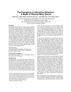
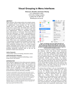
© Copyright 2026