
Experiment 24 THE TEMPERATURE DEPENDENCE OF
24 – i 2/1/2015 Experiment 24 THE TEMPERATURE DEPENDENCE OF RESISTANCE INTRODUCTION 1 A MICROSCOPIC ORIGIN FOR DC ELECTRICAL CONDUCTIVITY 1 THE MEAN FREE PATH 4 THE BAND STRUCTURE OF SOLIDS 8 Band structure basics 8 Conductors 8 SEMICONDUCTORS 9 Electrons and holes 10 Impurities and doping 11 EXPERIMENT APPARATUS 15 Resistance samples 15 Temperature sensor 16 Measurement and data acquisition 17 PROCEDURE AND ANALYSIS 18 Initial setup and familiarization 18 Cool-down to −40°C 19 Controlled warm-up to +110°C 20 Terminating the warm-up and beginning the overnight cool-down 20 DATA ANALYSIS 21 PRELAB PROBLEMS 22 APPENDIX A: SOME DETAILS OF THE THEORY Formation of energy bands in a solid 1 Thermal dependence of semiconductor charge carrier densities 3 Semi-classical charge carrier dynamics in a metal 5 APPENDIX B: DEGENERACY PRESSURE 24 – ii 2/1/2015 24 – 1 2/1/2015 THE TEMPERATURE DEPENDENCE OF RESISTANCE INTRODUCTION A steady (DC) electrical current is transmitted through a solid material by the bulk motions of mobile, charged particles (e.g. electrons) within it. The DC electrical conductivity of a solid material is an indicator of how abundant these mobile charges may be and how easily they can move within the material in response to an externally-applied electric field. The variation of this conductivity with temperature provides important clues to the nature of the fundamental dynamics and statistical behavior of a material’s molecules and the electrons they share (forming the bonds between them). In this experiment you will measure the temperature dependence of the DC electrical resistances of a few solids, including two archetypes of electrical behavior: metallic conductors and typical semiconductors. The DC resistances of the various samples will be accurately recorded over a temperature range of 233−383 Kelvin (−40°C to +110°C); by analyzing this data you will gain some insights into the surprisingly complicated behaviors of the charges within them. A MICROSCOPIC ORIGIN FOR DC ELECTRICAL CONDUCTIVITY It is a well-recognized fact that the application of a small, constant voltage ( V ) across a conducting material results in a proportional, steady current flow ( I ) in the circuit connected to it — this observation is, of course, embodied in what we call Ohm’s Law: V = I R , where the constant of proportionality, R, is called the element’s resistance. 1 We wish to develop a simple model for the microscopic origin of electrical conductivity in a solid which can explain this observed relationship. dl = vD dt I n, q, m E A J I Figure 1: A uniform, cylindrical, conducting wire carrying current I in response to an applied voltage V. The wire’s length is L and its cross-sectional area is A. The other quantities shown are defined in the text. Consider a conductor which has been formed into a long, homogeneous cylinder of length L and cross sectional area A (as in Figure 1). A battery applies the potential V, and current I flows 1 The Prussian (German) physicist Georg Ohm published the law named for him in 1827. It was based on experiments he conducted during his tenure as a high school teacher in Cologne. 24 – 2 2/1/2015 through the cylinder. The electric field within the wire is E = V L , and the current density (current area) inside the wire is J = I A . In terms of E and J Ohm’s law may be written: L1 I R = V → J = σ E, σ = A R (24.1) Thus Ohm’s law implies that the current density at a point in a conductor is proportional to the local electric field at that point; the constant of proportionality, σ, is called the conductivity. The reciprocal of the conductivity is known as a material’s resistivity: ρ ≡ σ −1 . For a good conductor (such as copper) resistivity is on the order of a few micro-ohm centimeters at room temperature (a good insulator, in contrast, would have a resistivity of at least 1020 times larger!). To proceed with an elementary microscopic theory of a solid’s σ (or ρ), assume that a solid metal or other conductor contains a cadre of identical mobile charges, called charge carriers (each of mass m and charge q), which may be accelerated by the application of an external electric field. These mobile charge carriers in a typical metal clearly come from the constituent atoms’ valence electrons (the most weakly bound electrons) — one or more of these electrons may be released by each atom as it forms chemical bonds with its neighbors. These electrons might then be able to roam relatively freely throughout the interior of the metal, leaving behind ions fixed in position by their bonds to their neighbors. The set of essentially immobile, relatively massive ions (whose charges balance those of the charge carriers) form a nearly rigid lattice — it is this ion lattice which makes the material a solid rather than a fluid. If the number density of the ions is N and they each contribute an average number Z of electrons to the pool of charge carriers (each with charge q = −e ) then the charge carrier number density n within the metal would be n = Z N . For example, copper provides one electron per atom, thus n= N= 0.85 ×1023 cm3 at 300K (using the atomic weight of copper and the metal’s mass density); this pool of charge carriers is collectively referred to as the metal’s set of conduction electrons. The application of an electric field to a conductor will accelerate the individual charge carriers, but thermal motions and random collisions within it might be expected to continually spoil what would otherwise be a coherent acceleration of the center-of-mass of the body of charge carriers. Assume that the net result of this thermal jostling will limit the average drift velocity of the charges in response to the applied field to be vD , a vector velocity parallel to and proportional to the local applied field E within the material. 2 It is this average drift of the charges which gives rise to the observed current density J within the material. Actually, we might expect that since a solid’s crystalline structure is not perfectly isotropic, vD generally need not be parallel to the applied field E . In this case we would talk about a conductivity tensor relating J and E in equation (24.1). We won’t consider this added complication here. 2 24 – 3 2/1/2015 Referring again to Figure 1, a net average drift velocity vD of the body of charge carriers implies that those within a distance dl = vD dt of the cross-sectional surface A will drift through it during time dt. If the charge carriers have number density n and charge q, then a total charge of = dQ qn = Adl qn AvD dt will cross the surface during time dt, giving rise to the current = I dQ = dt qn AvD . Thus the current density J is given by J = n qvD (24.2) This average drift velocity could be quite small in a good conductor, even when it carries a large current. For example, a copper wire with a 1mm2 cross-sectional area carrying a 1 Ampere current would require an average drift velocity of its conduction electrons of less than 0.08 mm/sec. In contrast, the random thermal velocities expected of the charge carriers should be much larger. If they were to behave as a classical gas of particles in thermal equilibrium with their surroundings and at temperature T, then their mean kinetic energy should be given by the equipartition theorem (see General Appendix B, Fundamental Concepts of Thermal Physics): 1 2 mv 2 = 32 k BT (24.3) ( k B is Boltzmann’s constant; k B × 300K ≈ 0.026eV, about 1 40 electron volt). For an electron, mc 2 = 0.511MeV (mega-electron volt), so at room temperature equation (24.3) would imply that the electrons’ equilibrium RMS thermal speed vT would be approximately vT c ≈ 4 × 10⁻⁵ → vT ≈ 12 km sec which is more than 100 million times larger than the average electron drift velocity vD estimated earlier. Quite obviously, we would therefore expect that vT vD for a typical metallic conductor. The charge carrier collisions which maintain their thermal equilibrium with the ion lattice must therefore be frequent and violent compared to the relatively modest acceleration applied by the external electric field E. Any evidence of drift due to an applied electric field (of order vD ) will be completely erased by a collision — the average velocity of a charge carrier immediately following a collision will be 0, although its average speed will be vT . We assume that charge carrier collisions with the ion lattice are random, independent, nearly instantaneous events compared to the mean time between collisions, τ. The probability that any given charge carrier will experience another collision in the next small time interval dt is equal to dt t , independently of how long ago its last collision occurred. Thus the probability that the charge carrier will avoid a collision over the next time interval t is equal to e−t t , and the mean time since its last collision is τ. Otherwise, between collisions a charge carrier’s motion evolves under the influence of externally-imposed fields. The mean time between collisions τ is also called the relaxation time because it determines the time scale over which the charge carriers’ temperature relaxes to its new equilibrium value after a change in the temperature of the ion lattice. 24 – 4 2/1/2015 Following a collision with the ion lattice, a charge carrier will be accelerated by the externallyimposed electric field: qE = m a. Since on average each charge carrier’s last collision occurred τ previously, at which time its average velocity was 0, the average drift velocity of the collection of charge carriers would be vD = a τ . Thus the equation (24.2) becomes J = q2 nq a n E = ττ m q2 σ = nτ m (24.4) Equation (24.4) is our first major theoretical result, known as the Drude relaxation time model of DC electrical conductivity. 3 Given our earlier calculation of= n 0.85 ×1023 cm3 in copper and ρ 1 σ ≈ 1.6 micro-ohm centimeters, copper’s its measured room-temperature resistivity of = corresponding relaxation time would be ≈ 3 × 10⁻¹⁴ sec. For comparison, this time equals the period of electromagnetic radiation with a wavelength of 1 micron: near-infrared light a bit beyond the red end of the visible spectrum (0.75 micron). It is the temperature dependence of (24.4) which we investigate in this experiment. THE MEAN FREE PATH Given an assumed mean time between collisions with the ion lattice of τ, we can similarly define the mean free path length λ traversed by a typical charge carrier between collisions to be λ = vTτ (we can safely ignore the effect of drift velocity vD in this expression because vT vD ). How can λ be expressed in terms of the physical nature of the solid? The charge carriers are scattered by interactions with various sites in the ion lattice. Some of these scattering sites could be essentially permanent locations in the lattice such as defects or grain boundaries of its crystalline structure; others could be, for example, the locations of particularly strong, momentary, random thermal vibrations of the ions in the lattice. A “collision” with the lattice would occur if a charge carrier is scattered (changes its velocity vector) by a large angle or its speed is changed by a factor of order unity. We assume that these scattering sites are uniformly but randomly distributed throughout the material with an average number density of nS (S for “scattering sites”). Assume that a charge carrier whose original, undeflected path would have it miss the center of a particular scattering site by distance b ≤ bS will experience a collision with the site (the distance b is called the impact parameter), but if its path would miss the scattering site center by more than bS then its trajectory is minimally affected (if at all). Thus if a charge carrier’s original trajectory would pass through a circular cross sectional area of σ S = π bS2 centered on a 3 The German physicist Paul Drude proposed his model for electrical conduction in 1900, three years after J.J. Thompson’s discovery of the electron. 24 – 5 2/1/2015 scattering site and normal to the carrier’s path, then a collision with the site results. The area σ S is called the total cross section for a collision event to occur (don’t confuse this σ S with the conductivity σ ). With these two general characteristics of the charge carrier-ion lattice scattering process (nS and σ S ) we can determine the mean free path λ. Consider the hypothetical situation shown in Figure 2 at right, in which a “beam” of charge carriers (all with the same velocity in the zˆ direction) passes through a thin disk of scattering sites oriented perpendicularly to the velocity vectors of the charge carriers; the emerging beam contains only those charge carriers which did not experience a collision with one of the sites in the disk. The number of scattering sites per unit area in the disk is nS dz , and their combined cross sectional area obstructs a fractional area nS σ S dz of the incoming beam. Thus only the fraction 1 − nS σ S dz of the incoming particles makes it through the disk without a collision. This then must be the probability that a single incoming particle will avoid a collision while traveling through an infinitesimal thickness of material containing scattering sites. dz Figure 2: A “beam” of charge carriers passes through a thin disk of fixed scattering sites. The emerging beam is weaker because some incoming particles collide with scattering sites in the disk. What this implies is that if P ( z ) is the probability that a charge carrier has already traversed a distance z through the material without a collision, then the probability that it makes it another dz farther is P( z + dz ) =P ( z ) + dP =(1 − nS σ S dz ) P( z ) , so dP dz = −nS σ S P( z ) . Integrating, P( z ) = e− nS σ S z . The mean distance a typical charge carrier will travel without a collision (the mean free path) is then the integral: ∞ = λ ∞ − nS σ S z ( z ) dz dz ∫0 z P= ∫0 ze = ∞ ∞ −n σ z dz ∫0 P( z )dz ∫0 e S S 1 = nS σ S λ (24.5) The mean time between collisions τ in expression (24.4) for the conductivity may be replaced with λ vT . Thus the temperature dependence of the mean free path, λ (T ), will clearly have a direct influence on the conductivity, σ (T ), so we now consider λ’s temperature dependence. Some ion lattice scattering sites may be characterized as a set of lattice distortions which are relatively fixed in size (σ S ) and number (nS ) , although some may be able to move about within the material. Examples of these sorts of charge carrier obstacles are crystal grain boundaries and certain types of crystal lattice defects. The efficacy of this class of scattering site is generally nearly independent of temperature, and its members may constitute the dominant scattering mechanism in relatively high-resistivity conductors such as alloys. The dominant scattering mechanism in high-conductivity metals and carefully-prepared crystals, on the other hand, is due to thermal motions of the ions in the lattice, and these motions are clearly going to depend on the temperature (the thermal origin of these motions are, naturally, 24 – 6 2/1/2015 also a very important factor in determining a solid’s heat capacity and thermal conductivity, as well as determining its expansion and contraction with temperature). The normal modes of vibration of the ion lattice consist of compression waves and transverse waves of various wavelengths and frequencies. As does a quantum harmonic oscillator, a lattice vibrational mode with resonant frequency ω0 would have quantum energy levels separated by increments of ω0 . The low-frequency modes (ω0 < k BT ) will be subject to the statistical-mechanical equipartition theorem when the solid is in thermal equilibrium, so the average energy stored in the lattice by each such mode will be proportional to temperature. 4 To estimate the effect of the thermal energy stored in the lattice vibrational modes on their ability to scatter a conductor’s charge carriers, we can think about it this way: the squared displacement amplitude of the vibration in a particular mode is proportional to its energy (to first order), which, on average, is proportional to T. The cross section for a collision of a charge carrier with this lattice distortion (σ S ) has units of area, and so should also vary as the square of the displacement amplitude (which has units of length). Thus, one would expect that σ S ∝ T for each such mode. The number of lattice normal modes is determined by the number of atoms in the lattice, 5 so we may assume that nS is at most a weak function of T for these thermal modes, except perhaps near the solid’s melting point. Thus, for the thermally-induced vibrations of the lattice nS σ S ∝ T , at least over a moderate temperature range well below the conductor’s melting point. Considering collisions with both the thermally-induced lattice distortions and those more permanent sites associated with dislocations, impurities, and the like, we may conclude that the overall collision cross-section, nS σ S , should be approximately linear in T: −1 λ= nS σ S ≈ a + bT (24.6) for some constants a and b, at least for temperatures far from the material’s melting point. In the case of carefully-prepared crystals or good conductors, the term proportional to T should dominate; for high-resistivity alloys or amorphous materials, the constant term may be the dominant one. What this implies is that for a good conductor, its conductivity will have a factor inversely proportional to T. 4 Actually the collection of all of these various lattice vibrational modes supports the propagation of wave packets of vibrations (as with waves on an elastic string). A wave packet with dominant frequency ω0 and energy ω0 is called a phonon (analogous to a photon). Phonons are, like photons, bosons: particles which are described by BoseEinstein statistics. The equipartition theorem will only apply when the density of phonons with a given frequency is so low that they are (on average) separated by distances much larger than the sizes of their wave packets. 5 If N is the number of atoms in the lattice, then 3N is the number of vibrational normal modes. To see why this is so, note that each atom’s position has 3 degrees of freedom, so there are 3N mechanical degrees of freedom for the atoms in the lattice, but this must also equal the number of normal modes, since each mode corresponds to a single degree of freedom. 24 – 7 2/1/2015 Two important points to remember about our discussion leading up to (24.6): first, we have claimed that charge carrier scattering by the ion lattice is associated with lattice distortions and not by direct scattering from the individual ions. In fact, it turns out that a metal with a flawless crystal lattice with perfect periodicity can have infinite conductivity: the energy eigenstates of the conduction electrons may be constructed from traveling waves with the same periodicity as the lattice. Thermally-induced lattice vibrations and crystal defects spoil this ideal scenario, however, so real crystals exhibit some resistance to conduction electron flow. 6 Second, the vibrational modes of the lattice are, of course, quantized as mentioned above, so the energy of a mode with frequency ω0 may only be changed by increments of ω0 . If ω0 > k BT , then it is unlikely that the mode will be excited from its ground state by thermal processes (such a mode is said to be frozen out). An estimate of the temperature required to excite the highest frequency mode of the lattice (with wavelength ≈ the interatomic spacing) is given by the Debye temperature, Θ D (after the Dutch-American physicist Peter Debye). For copper Θ D ≈ 315 K , so a few of its very highest vibrational modes may be frozen out during this experiment. At temperatures T Θ D , the freezing out of modes and the small energies associated with the remaining modes combine to increase a good conductor’s mean free path at a much faster rate with decreasing temperature: roughly approaching λ ∝ T −5 . At very low temperatures scattering is then dominated by the relatively permanent lattice deformations mentioned above. Returning to our previously derived expression for the conductivity, we can replace the relaxation time τ with λ vT , and then explicitly include λ’s temperature dependence from (24.6): = σ q2 n λ = m vT q2 n m vT (a + bT ) (24.7) Thus we expect that the resistance, which is proportional to σ −1 , should have a factor linear in the temperature T. The other factors n and vT , may each have their own individual temperature dependence, as will be investigated in the next section. 6 Except, of course, for the low-temperature phenomenon of superconductivity, whose origin is completely different from the motions of the conduction electrons described here. 24 – 8 2/1/2015 THE BAND STRUCTURE OF SOLIDS To complete our theory of the temperature dependence of the electrical conductivity given by equation (24.4), we must investigate the variations with temperature of the charge carrier number density n and the average random charge carrier speed vT . To construct such a theory, we must consider the quantum-mechanical nature of the electrons in a solid — in particular, the structure of the energy levels they may occupy. Band structure basics A complete quantum mechanical theory of electrons in a solid would be, as one might expect, complicated and subtle. Here we summarize the features of the theory which are relevant to our study of DC electrical conductivity: 1. The single-electron states in a crystalline solid are organized into a set of energy bands, with each band corresponding to a single electron orbital of an isolated constituent atom or molecule of the crystal. Each band contains a total of 2N single-electron states per unit volume, where N is the number density of ion lattice sites in the crystal. 2. A typical energy band has a total width of a few to several electron volts (eV), and different bands may be separated by a similar energy, although some bands may overlap. The separation between two bands is called the energy gap ε G (we use the symbol ε for energy to avoid confusion with the electric field strength E). 3. Electrons are fermions, so a maximum of only one electron may occupy any particular state. At temperature T = 0 (absolute zero, when the system is in its ground state), the electrons fill the available single-electron states in the various energy bands starting with the lowest energy state in the lowest energy band. At temperatures T > 0 the electron distribution among the various states (occupation probabilities) is given by the Fermi distribution, f (ε ), described in General Appendix B, Fundamental Concepts of Thermal Physics. 4. A completely full or completely empty energy band does not contribute to the electrical conductivity of the solid; only the electrons in partially-occupied bands may act as mobile charge carriers. Different partially-occupied bands conduct current independently of one another, and the total conductivity of the solid is given by the sum of the conductivities provided by these bands. Solids with no partially-occupied energy bands are insulators (or, possibly, semiconductors); conductors (mostly metals) have at least one partially-occupied energy band (even at T = 0). Conductors If some bands are partially-occupied at T = 0, then the energy of the highest occupied level is called the Fermi energy, EF . Typically this energy may be a few to several eV from the bottom of the partially-occupied band; in this case it is useful to measure EF from the nearest band edge. 24 – 9 2/1/2015 In the case of copper the electron density is= n 0.85 ×1023 cm3 in its partially-occupied band. Because this density is so high, the majority of these electrons occupy states with f (ε ) ≈ 1, and their nearby states (∆ε kBT ) are very probably occupied as well. Thus these electrons behave as a degenerate Fermi gas, so their quantum characteristics play a major role in determining their collective behavior. For example, a gas of free and independent electrons at this density would have EF = 7.0 eV (compare this to the room temperature k BT ≈ 1 40 eV), and in the ground state (T = 0) the average kinetic energy per electron should be approximately (3 5) EF ≈ 4 eV (General Appendix B equation B.18). Clearly, the kinetics of a metal’s conduction electrons with these densities can be expected to be completely different from that prescribed by classical statistical mechanics, particularly the equipartition theorem used in equation (24.3). 7 What does not change, however, is the fact that the application of an external electric field can exert only a tiny perturbation on the velocity vectors of all but a handful of the electrons in the band, i.e. it remains true that vT vD , where vT is the average random speed of those electrons carrying the electric current within the conductor. As it turns out, the current through such a conductor is actually carried by those electrons within a few k BT of the Fermi energy EF , and, as long as EF k BT , the volume number density of these electrons is very nearly independent of temperature. In fact, the conductivity of a metal such as copper may be approximated by assuming that essentially all of the partially-occupied band’s electrons are collectively carrying the current as though they all had random kinetic energies of ≈ EF . Consequently, in expression (24.7) for the conductivity σ, the charge carrier density n and their thermal speed vT should be nearly independent of temperature, so that a metal’s resistance should depend only on the temperature variation of the mean free path λ; thus a metal’s resistance should vary approximately linearly with temperature T. SEMICONDUCTORS Semiconductors have electrons occupying only completely filled bands (at least at cold temperatures), characteristic of insulators. What makes them different, though, is that the bottom of the nearest empty energy band (called the conduction band) is only about an electron volt or so away from the top of the highest-energy filled band (the valence band). Consequently, random thermal jostling of the ions in the lattice can very occasionally impart enough energy to an electron near the top of the valence band to excite it into a level near the bottom of the conduction band. In this case both the valence band and the conduction band become partially occupied (although just barely), and the material becomes a poor conductor (poor because only a 7 Arnold Sommerfeld, the German physicist, modified Drude’s theory of metals to incorporate the Fermi distribution of electron energies in 1927. A great physicist and teacher, Sommerfeld’s students went on to win seven Nobel prizes, including Werner Heisenberg, Wolfgang Pauli, Linus Pauling, and Peter Debye. 24 – 10 ni ∝ T 3 2 e − Eg (2 kBT ) (24.8) where Eg is the magnitude of the energy gap between the valence and conduction bands. In the case of silicon, this amounts to on the order of 1010 electrons per cm3 at room temperature (compare with copper’s 1023 per cm3). The archetypal semiconductors are the elements silicon ( Eg = 1.12eV ), and germanium ( Eg = 0.67eV ), each of which forms a diamond crystal lattice with four covalent bonds per atom. Several compounds and alloys form commercially important semiconductors, including GaAs, InP, GaAsP, and InGaN. Conduction band − Occupation Density of states Egap tiny fraction of the valence electrons get bumped up into the conduction band). The higher the temperature, the greater the number of valence electrons thermally excited into the conduction band — the number goes as: 2/1/2015 + Valence band Figure 3: Densities of states and occupations by electrons (conduction band) and holes (valence band) for a pure semiconductor (intrinsic charge carriers only); energy increases in the vertical direction. Unlike the case of a metal’s conduction electrons, the number densities of a semiconductor’s conduction electrons and holes (defined below) in their respective bands are low (much smaller than the crystal’s atomic number density N ). Therefore, Pauli Exclusion plays only a minor role in the kinematics of these low-density fermions, so a semiconductor’s charge carriers will distribute themselves in a way very accurately described by the classical Maxwell distribution, and the overall occupation densities go as the left-hand curves in Figure 3. Electrons and holes The diagram in Figure 3 illustrates the distribution of electrons near the bottom of the conduction band and the distribution of unoccupied single-electron states near the top of the valence band for a semiconductor at a fairly high temperature. The Boltzmann factor exp(− ∆E k BT ) gives the relative probability that any one state is occupied in the conduction band or unoccupied in the valence band, where ∆E is the magnitude of the difference in energy between the state and its band edge, and the dynamics of the relatively small number of electrons in the conduction band is quite accurately approximated by treating them as classical particles (with a negative charge of −qe , of course). In the valence band only a small fraction of the states near its top are unoccupied. Interestingly, the dynamics of the remaining electrons near the top of the valence band are such that they have a negative effective mass, since the density of states increases with decreasing energy near the top of the band (the concept of the effective mass m* of a charge carrier is described in this experiment’s Appendix A). The consequence of this unusual electron behavior near the top of 24 – 11 2/1/2015 the valence band is that the unoccupied quantum states evolve as though they were occupied by positively charged particles (+ qe ) with a positive effective mass and with energies increasing as they move further down from the band top in an otherwise empty band! These “positive charge carriers” near the top of the valence band are called holes. In fact, the behaviors of holes near the top of a semiconductor valence band are completely equivalent to those of “real” particles such as the conduction band electrons, so their particle nature is just as valid. Thus, when an electron is excited from the valence band to the conduction band, two charge carriers are created: the electron (−qe ) and the hole it left behind (+ qe ). 8 Since the energy an electron must gain to cross the energy gap between the valence and conduction bands is at least Eg , but two particles were created by this transition, the required energy per particle is Eg 2 — this is a convenient “handwaving” explanation of the extra factor of 1 2 in the Boltzmann expression (24.8). According to our original derivation of the conductivity, equation (24.4), the conductivity of a semiconductor band is proportional to the volume density of its charge carriers (electrons in the conduction band, holes in the valence band); thus a pure semiconductor has a conductivity which is a very strong function of temperature, rising rapidly as temperature increases, as indicated by expression (24.8). This effect is used to make a thermistor: a resistor with a large, negative temperature coefficient (decreasing resistance as temperature rises) which acts as a very sensitive, fast-acting temperature sensor for the range of about −100°C to +150°C. Using measured values for the effective electron and hole masses and the band gap energies, using Appendix A equations (24.A.5) through (24.A.7) will give the ionization fraction (ni N ) of the intrinsic semiconductors germanium and silicon at 300K to be: = ni (T 300K) N Ge ≈ 5.4 ×10 −10 = ni (T 300K) NSi ≈ 3.0 ×10 −13 (24.9) As can be seen from these numbers, at room temperature the probability that an individual valence electron is thermally excited across the energy gap and into the conduction band in one of these semiconductors is incredibly tiny — typically smaller than, for example, the chances of a particular holder of a single ticket winning a major state lottery jackpot. Impurities and doping Semiconductor materials are custom-made to be much more flexible and useful through the process of doping: introducing various amounts of impurity atoms into the semiconductor crystal which have a valence different from that of the semiconductor. For example, mixing a small amount of phosphorous (valence 5) into a silicon crystal will introduce a random distribution of 8 Interestingly, even a metal with a partially-filled conduction band may have charge carriers more appropriately characterized as holes with charge + qe . This “anomalous” sign of the metal’s charge carriers is detectable in experiments measuring the Hall effect in a magnetic field. For example, aluminum’s charge carrier density in the presence of a large magnetic field is best described as having one hole per lattice ion. 24 – 12 2/1/2015 atoms each with an extra valence electron left over after it forms bonds with surrounding silicon atoms. What would be the consequences of these extra electrons to the physics of the material? It turns out that the energy of this extra valence electron is very close to the energy of the bottom of the conduction band (in the case of P in Si, the energy is only 0.044 eV below the conduction band). If there are relatively few of these donor impurity atoms, then it is very likely that such electrons will eventually be excited into the conduction band by the thermal motions of the ions: once there they quickly drift away from their parent impurity atoms and are unlikely to recombine with them. So even if the ambient temperature is so cold that almost no electrons would be excited from the valence band to the conduction band, electrons from donor impurities will nearly all eventually find their way into the conduction band, providing a largely temperature-independent cadre of negative charge carriers (−qe ) along with the same number of fixed, positively-charged ions distributed throughout the crystal lattice. Such a material is called an N-type semiconductor. Similarly, introducing a valence 3 impurity atom (such as aluminum into silicon) will leave an unsatisfied bond because of the missing electron. Again, the energy required to promote a nearby silicon valence electron into this spot is small compared to the semiconductor’s energy gap (0.057 eV for Al in Si). Thermal agitation will eventually do the trick, and the vacated valence state becomes a hole which quickly drifts away from the impurity atom, trapping the promoted electron at the impurity site. Thus these acceptor impurity atoms become fixed, negativelycharged ions in the lattice, whereas an equal number of holes form a nearly temperatureindependent group of positive charge carriers (+ qe ) , creating a P-type semiconductor. Adding impurities to a semiconductor can not only introduce charge carriers (called extrinsic charge carriers), but will also suppress the thermal creation of electron-hole pairs described by equation (24.8), called intrinsic charge carriers. This is because the product of the number densities of the conduction electrons (nc ) and holes ( pv ) is related to the number density of the intrinsic charge carriers that would be thermally created in a pure (undoped) semiconductor (ni ) by the laws of statistical mechanics: nc pv = ni 2 (24.10) For example, the addition of 1 part per million phosphorous (a donor impurity) to a silicon crystal ( N d N = 10−6 ) would introduce 5 × 10¹⁶ conduction electrons per cm3, making the material an N-type semiconductor. With ni N about 7 orders of magnitude smaller at room temperature (24.9), equation (24.10) would require that there be only pv 5000 holes per cm3, 13 orders of magnitude smaller than nc ! These holes are called minority carriers in the N-type silicon under discussion; the conduction electrons are the majority carriers. As the semiconductor’s temperature rises, ni and thus the minority carrier number density will eventually become comparable to that of the extrinsic charge carriers; as the temperature is raised even further the extrinsic carrier population becomes an ever less important contributor to 24 – 13 2/1/2015 the overall charge carrier density, and the electron and hole densities both approach ni . At this point the charge carrier variation with temperature is well-described by (24.8). The conductivity of a semiconductor depends on the total charge carrier density nc + pv since both the conduction and valence bands can conduct electrical current. In the case of a pure 2ni , so the charge carrier density will vary with temperature as given by semiconductor nc + pv = (24.8). Introducing extrinsic charge carriers by doping the semiconductor with impurity atoms, however, complicates the situation. For the sake of argument, assume that the semiconductor is N-type with donor number density N d , and assume that the temperature is high enough that all but a negligible fraction of the donor impurity atoms are ionized. Since the only other source of electrons in the conduction band is from ionization of the intrinsic semiconductor atoms nc N d + pv . With this expression (creating an equal number of holes), it must be the case that = and equation (24.10), the total charge carrier density must be: n = nc + pv = N d 2 + 4 ni 2 (24.11) Expression (24.11) makes it clear that, as expected, at low temperatures when ni N d , then n → N d ; when the temperature is high, then n → 2ni . The thermal variation of (24.11) is contained in ni (T ), given by (24.8). Figure 4 shows how n varies with temperature for various levels of impurity concentration in germanium. Figure 4: Relative charge carrier density n N v. temperature given by equation (24.11) for germanium with impurity concentrations of 0.1 to 10 parts per billion. The intrinsic ionization fraction ni N is given by (24.9) at room temperature and varies with temperature as in (24.8). 2 ni N is shown by the dashed line. Because of the low densities of the conduction electrons and holes in their respective bands, their velocity distributions will be fairly accurately described by the classical Maxwell distribution of an ideal gas of particles at temperature T. 9 Thus their average thermal speeds will vary with temperature as vT ∝ T 1 2 , as shown in expression (24.3), with masses given by their respective effective masses, m* (defined in this experiment’s Appendix A). Since the crystals used to create doped semiconductor materials are usually of very high quality, the mean free path λ of a charge 9 With two major differences from a classical ideal gas: (1) they reach thermal equilibrium through collisions with the ion lattice and not through collisions among themselves; and (2) their number density n is in general a strong function of temperature T. 24 – 14 2/1/2015 carrier should vary as T −1. (cf. equation (24.6)). Consequently, the relaxation times of the conduction electrons and holes should vary with temperature as in equation (24.12). = τ λ vT ∝ T −3 2 (24.12) Thus a semiconductor’s conductivity σ, which from (24.4) varies with the product n τ , should display an overall temperature variation given by the product of (24.11) with (24.12), according to the simple theoretical model presented here. Figure 5: Plots of the theoretical temperature variation of the resistance of a doped semiconductor (germanium, with E g = 0.67eV ). The doping level is such that N d= 10 × ni (300K). Left: conventional plot of R v. T; right: plot of log ( R ) v. 300K T . Also shown are the asymptotic purely extrinsic ( N d only) and purely intrinsic behaviors (dashed lines). These asymptotic curves cross where N d = 2 ni . Figure 5 shows the expected temperature variation of the resistance of a typical doped (impure) semiconductor according to the theory presented here ( R ∝ 1 nτ , with n and τ given by equations (24.8), (24.11), and (24.12)). The theory is plotted two different ways; each plot has its advantages when analyzing a data set. 24 – 15 2/1/2015 EXPERIMENT APPARATUS A B C D E F G H Figure 6: The experiment apparatus, with a schematic diagram of its various components. A: data acquisition unit; B: heater power control; C: stirring motor; D: insulated flask containing dielectric fluid; E: platinum temperature sensor; F: array of samples under test; G: fluid stirring paddle; H: resistors used to heat the fluid. The apparatus used for the experiment is shown in Figure 6. The heart of the system is its array of resistance samples along with a platinum temperature sensor (F and E in Figure 6 and also shown in the photo in Figure 7 on the next page). Measurement of the resistance values and the temperature is accomplished by a precision data acquisition unit operated under computer control. The samples are immersed in a dielectric (electrically insulating) fluid contained in a vacuum-insulated flask. A paddle attached to a motor continuously stirs the fluid so that its temperature is kept uniform as it flows around the samples and a set of resistors used as a heating element (H in Figure 6). The circulating fluid acts as a heat bath which transfers heat to the samples and the temperature sensor to keep them all at a common temperature. After initially cooling the fluid using liquid nitrogen (LN2), the fluid is then heated by the power dissipated in the heater resistors while the data acquisition unit periodically measures and records the temperature and the corresponding sample resistances. Resistance samples The five resistance samples are attached to a rigid framework of stainless steel rods and acrylic spacers as shown in the photo in Figure 7. The framework is immersed in the bath of dielectric fluid which keeps the samples in thermal equilibrium with it and each other (as long as the bath 24 – 16 # # # # # 2/1/2015 Resistivity Experiment v3.0 Data Acquisition Unit: Agilent Model 34970A Start Time: 3:20:12.014 PM 1/24/2014 ; Start Temp: 232.1530 K Time (s) Temp (K) R1 R2 R3 R4 0.000000 232.1530 757.5709 2735.109 4.193582 1393884 53.86600 233.1510 762.7967 2732.739 4.214232 1304626 94.63900 234.1900 768.3800 2730.243 4.236844 1186270 136.3170 235.2280 774.0844 2727.689 4.259203 1109731 176.2270 236.2380 779.4262 2725.294 4.280990 1042045 218.6790 237.2790 785.1033 2722.823 4.304552 976368.1 C R5 26.86568 26.86892 26.87157 26.87405 26.87690 26.87810 A B D E F Figure 7: An example of the data file output (left) and the array of samples (right). A: semiconductor (R1); B: platinum temperature sensor; C: coil of manganin wire (R5); D: commercial precision carbon film resistor (R2); E: thermistor (R4); F: coil of copper wire (R3). temperature does not change too rapidly). Each sample is attached to the data acquisition unit by a network of four wires as will be explained in a later section. The various samples are identified by the computer data acquisition program as resistors R1 through R5 as shown in Table 1. The sample output data file shown in Figure 7 demonstrates how the resistance data are organized for further analysis. Table 1: Resistance Samples R1: Semiconductor rod R2: Commercial resistor R3: Copper wire R4: Thermistor R5: Manganin wire Temperature sensor The temperature sensor is a precision platinum resistive temperature detector (RTD) with a design resistance of 100Ω at 273.16 Kelvin (the triple point of water, 0.01°C). It is designed to meet the specifications of the international standard known as IEC 60751 Class A, which requires that its temperature measurement error be less than ±(0.15K + 0.002 × T − 273.16K ), which is less than ±0.37K over the temperature range of this experiment. Details of its specifications are available at: http://www.sophphx.caltech.edu/Lab_Equipment/RTD_temperature_probe.pdf The RTD sensor (shown as element B in the photo in Figure 7) has a small thermal mass and a relatively large surface area, so its temperature will remain very close to that of the surrounding dielectric fluid as the experiment proceeds. Because platinum is a good metallic conductor, its resistance changes very nearly linearly with temperature. The standard temperature coefficient of 24 – 17 2/1/2015 resistance (called α) specified for the platinum alloy used is 3.85 mΩ Ω K (at 0°C), so a sensor with a 0°C resistance of 100.0Ω should measure 138.5Ω at 100°C. Measurement and data acquisition The resistances of the samples and the platinum RTD are measured by an Agilent (now Keysight Technologies) model 34970A Data Acquisition / Switch Unit (DAQ) with an installed 34902A multiplexer module. This device contains a precision digital multimeter which performs the resistance measurements; the multiplexer module contains relays which connect the various samples to the multimeter. A program stored in the unit controls the sample selection and measurement process; data are transferred to a host computer using the device’s GPIB interface (also known as an IEEE-488 interface). The User’s Guide for the DAQ is available here: http://www.sophphx.caltech.edu/Lab_Equipment/Agilent_34970A_User_Manual.pdf The preset, internal DAQ program for this experiment commands it to continually monitor the platinum RTD resistance and determine the dielectric fluid temperature while in its idle state, and the instrument displays the measured temperature in °C on its front panel. When commanded by the host computer, the DAQ momentarily leaves this idle state and executes its measurement program, cycling through the RTD and the resistance samples and reporting the temperature and resistance measurement data to the host computer for display and recording. The resistance measurements of both the samples and the RTD are accomplished using the 4wire ohms measurement technique described starting on page 291 of the DAQ User’s Guide (link above). Two wires are used by the DAQ to apply a known, precision current through the sample; two separate wires, attached across the sample, connect the DAQ’s precision voltmeter to it. This method removes the wiring resistance from the measurement, resulting in a more accurate result, especially if the sample has a relatively small resistance (as do the RTD and the copper sample). 24 – 18 2/1/2015 PROCEDURE AND ANALYSIS The procedure for this experiment divides naturally into 4 distinct phases: 1. 2. 3. 4. Initial setup and familiarization. Cool-down to −40°C. Controlled warm-up to +110°C and primary data acquisition. Overnight cool-down to room temperature and secondary data acquisition. Each of these phases is discussed below. Initial setup and familiarization Start the Resistivity application program; if the data acquisition unit is properly connected to the host computer, then the software should successfully initialize. The main control window for the program is shown in Figure 8 at right. Turn on the program’s context help window (selected using the Help menu) and hover over the various controls for a description of their operation. The DAQ unit should display the fluid temperature in degrees Celsius, which should be within a few degrees of room temperature. Start the stirring motor and adjust its speed so that the fluid is stirred just strongly enough to see motion of the fluid surface; don’t stir so hard that large waves and bubbles appear in the fluid (you aren’t making a smoothie, after all). Figure 8: The main control window of the Resistivity application software. The heater should be turned off, and the cooling fan should be disconnected and removed from the top of the apparatus. Set the trigger mode to Time with an interval of around 1 second. Specify a new data file name to the control program and acquire several data points. Examine the data for the temperature and various sample resistances using the Data Plots window. You will use this data to estimate the noise levels in the various measurements which you may then assign as uncertainties to your data. 24 – 19 2/1/2015 Cool-down to −40°C Read through this section completely before beginning the cool-down process. You will cool the dielectric fluid by slowly pouring small amounts of liquid nitrogen (LN2) into the flask using a funnel. The very cold LN2 will boil vigorously when it contacts the fluid, whereas some of the fluid will freeze. As long as the frozen fluid layer doesn’t get too thick and extensive, the stirring motor will continue to circulate warmer fluid to the frozen surface, causing the layer to melt. DO NOT pour in a large quantity of LN2 all at once! Pouring a large amount of LN2 into the dielectric fluid will cause very strong splashing and atomizing of the fluid. These vapors will spread a film of fluid over all nearby surfaces, including you! The fluid is not a health tonic! If the motor stalls because of ice buildup around the shaft to the stirring vane, twist the shaft using your fingers to attempt to free it. If this proves to be impossible, then unplug the stirring motor and fetch the lab instructor! It should take 15 minutes or so to reduce the fluid temperature to the −40°C target. As the fluid gets colder, it will take longer for the surface ice to melt. Always wait for nearly all of the ice to melt before introducing more LN2. As the displayed temperature passes through −35°C, wait for the temperature to become reasonably stable before adding each subsequent dose of LN2. By acquiring a data set and watching the temperature v. time graph, you will be able to tell when the rate of change of the fluid’s temperature becomes small as the fluid and samples approach thermal equilibrium. Don’t start the warm-up phase until the samples and fluid are near this equilibrium. Figure 9: Cooling the dielectric fluid using LN2. 24 – 20 2/1/2015 Controlled warm-up to +110°C Name a new data file for your primary data set and configure the data acquisition to be triggered by a temperature change of about 0.5K to 1.0K. The heater resistors immersed in the dielectric fluid are powered from the 120VAC power line using a Variac® autotransformer. The single-winding autotransformer does not isolate its output from the 120VAC source, so be careful to not touch any exposed conductors attached to it. Once the temperature of the fluid has stabilized near −40°C, begin the warm-up by turning on the Variac and setting its output voltage to 130V. The Variac’s connection to 120VAC power is through a timer which will shut off power to the heater when it times out. Set the timer to 3 hours and activate its output; your TA can assist you if necessary. Start the data acquisition and make sure that the temperature is increasing by monitoring the temperature plot. As the temperature rises, periodically check the various resistance plots and consider the variations v. temperature they begin to define. The data file is opened, rewritten, and closed following each data point acquired by the DAQ, so you can open it using CurveFit at any time during the data acquisition to attempt some preliminary data analysis in lab. Also spend this time reviewing the theory presented by these notes so that you are thoroughly familiar with its concepts and the resistance variation expected for a good conductor and for a semiconductor. Do not allow the fluid temperature to exceed +110°C. Terminating the warm-up and beginning the overnight cool-down Turn off the heater Variac as the fluid temperature just reaches +110°C, and then terminate the data acquisition. Ask your TA or the lab administrator to show you how to rig the cooling fan atop the fluid flask and connect its power cord to begin cooling the fluid. Do not overwrite your warm-up data file with the cool-down data! Identify a new data file and configure the data acquisition to trigger on a time interval of about 100 seconds. Begin the data acquisition; this cool-down period will continue overnight unless another lab section requires the experiment apparatus sooner. The lab administrator will terminate this data acquisition the following weekday morning. Because the file is rewritten and saved for each data point, you will not need to access the application program to retrieve this final data set. Double-check that the heater Variac is turned off. Thoroughly wash your hands when you are finished to remove any traces of the dielectric fluid. 24 – 21 2/1/2015 DATA ANALYSIS The primary objectives of your data analysis for this experiment are to: (1) Test the theoretical model for the temperature dependence of the conductivity of a good conductor (boxed paragraph on page 9) using the copper resistance data. (2) Test the theoretical model of the conductivity of a semiconductor (boxed paragraph on page 14) using the thermistor resistance data (pure semiconductor) and the semiconductor data (doped semiconductor). Byproducts of your analysis should include accurate estimates (with uncertainties) of: (1) The temperature coefficients of resistance at 0°C and 20°C of the copper sample; your 20°C value should be compared to the published value for annealed copper wire. 10 (2) The gap energy (in eV) of the thermistor’s semiconductor material. (3) The gap energy (in eV) and doping concentration (fraction of atoms which are dopants) for the semiconductor rod sample. Determine which semiconductor (silicon or germanium) is most likely the material making up the sample. In addition, thoughtful, mainly qualitative comments regarding the other two samples, the commercial resistor and the manganin wire, should be made. Uncertainty estimates (error bars) due to noise in the measurements may be derived from an analysis of the initial data you obtained prior to the LN2 cool-down. The overnight cool-down data may be compared to the warm-up data to estimate the magnitude of systematic errors in the sample temperature measurements due to temperature gradients between the samples and the dielectric fluid. Of course, the systematic calibration uncertainties of the temperature probe and the resistance measurements will introduce additional uncertainties into the determination of the copper coefficient of resistance and to the gap energies of the semiconductors. Include these additional uncertainty sources in your parameter value estimates. Specifications of the instruments may be found in documents located here: http://www.sophphx.caltech.edu/Lab_Equipment/ . Many simplifications were made in deriving the theory presented here of the temperature variation of DC electrical conductivity. Do you see evidence which may indicate that these simplifying assumptions overlook effects present in your data? 10 The temperature coefficient of resistance at temperature T0 (also called α) is defined to be: α≡ 1 dR R(T0 ) dT T0 24 – 22 2/1/2015 PRELAB PROBLEMS 1. What would be the speed of conduction electrons with kinetic energy equal to copper’s Fermi energy of 7eV? Assume that these electrons behave as though they were free and independent, and that their effective mass is equal to the mass of a free electron (i.e., mc 2 = 0.511MeV). What would be the conduction electron number density in cm−3? You might want to review General Appendix B, Fundamental Concepts of Thermal Physics. 2. If the resistivity of copper at room temperature is 1.6 micro-ohm centimeters, and given the mass and number density from problem 1, then according to the simple conductivity model presented in the text, what should be the relaxation time τ ? If the charge carriers are moving at the speed you calculated for copper’s Fermi energy of 7eV, then what would be the charge carriers’ mean free path λ in Angstroms (Å)? How does this compare to the interatomic spacing of 2.55Å? 3. One of the resistance samples is a coil of Manganin wire. Look up the composition of this alloy of copper. How does its published resistivity compare with copper’s 1.6 micro-ohm centimeters? Would you expect Manganin to show a variation of resistance with temperature which is greater than, less than, or about the same as that for copper? Why? 4. Derive expression (24.11) on page 24-13 for the total charge carrier density n in a semiconductor. Consider the discussion in the text leading up to that equation along with equation (24.10). Show that (for an N-type semiconductor) the conduction electron and hole densities are: 1 nc = 2 ( n + N d ) (24.13) 1 pv = 2 ( n − N d ) where n is given by (24.11). 5. Assume a thermistor is constructed from a crystal of pure semiconductor (intrinsic charge carriers only) with an energy gap Eg = 0.6 eV. What should be the approximate ratio of its resistance at −40°C to its resistance at 110°C? 6. What is the published temperature (the boiling point) in Kelvin of liquid nitrogen (LN2) at standard atmospheric pressure? How does this compare to the minimum experiment test temperature of −40°C? 24 – A – 1 2/1/2015 APPENDIX A: SOME DETAILS OF THE THEORY Formation of energy bands in a solid The conduction electrons in a solid aren’t really free, of course, because they must move about in the generally periodic electric potential of the ion lattice. Consider this thought experiment: position a huge number N of atoms such as copper into an array with the same structure as found in their crystalline solid state, but with their atomic separations increased by a few orders of magnitude. Because of the atoms’ large separations from each other in this initial configuration, the individual, electrically neutral atoms would behave quite independently of each other, and their electrons will be confined to the atomic orbitals expected for a single, isolated atom. An array of wave functions of a particular atomic electron orbital over the entire assemblage of atoms would form a function with the overall periodicity of the atomic array, but, because of the large atomic separation, the amplitudes of these wave functions would very nearly vanish in the large volume between the various atoms. Since each electron orbital in an atom corresponds to two electron states (spin up and spin down), any particular assemblage of atomic orbitals could accommodate a total of 2N electrons (we ignore the effects of spin-orbit coupling on the wave-functions). Now consider what would happen as the array of atoms is slowly and uniformly compressed, so that the atomic separations gradually approach their values found in an actual solid. As the atoms grow nearer, the wave functions of the outer (valence) electrons will start to overlap those of each atom’s nearest neighbors. Consequently, the electrons in these states will start to experience significant additional electrostatic forces, not only from the atoms’ nuclei but also from each other. These outer orbitals’ states will begin to mix ever more strongly as the atoms get closer (meanwhile, the much more compact inner electron orbitals will still remain well-separated and essentially distinct). This overlap of the original, outer atomic orbitals implies that the actual wave-functions for these states must change as the atoms get near each other. The states will no longer be identifiable with a single atom, but will require that electrons occupying them be associated with several nearby atoms. This mixing, of course, is the origin of the chemical bonds between the atoms. As far as our crystalline solid is concerned, there will still be a total of 2N distinct electron states associated with each original array of corresponding atomic orbitals, and the modified states will still share in the periodicity of the crystal lattice. The energies of these new states, however, will generally be split into many nearly equal but distinct values, so that what was originally a common, single energy value for the states when they were associated with separate, identical atomic orbitals becomes a band of distinct wave-functions with closely-spaced energies, the band becoming wider as the atoms get closer. 24 – A – 2 2/1/2015 Thus a set of bands of distinct wave-functions will form in the solid, one band corresponding to each of an isolated atom’s atomic orbitals (or to each member of some complete set of linear combinations of these orbitals). The width in energy of a typical band is on the order of a few to several electron volts (the same order of magnitude as the binding energy of a valence electron in one of the atoms), and adjacent bands associated with the valence electrons are often separated by a similar energy, although they may also overlap (depending in a complicated way on the geometry of the crystal structure and the nature of the material’s interatomic bonds). The wave-functions of the energy eigenstates in these various bands in a crystal may be chosen to be plane waves with well-defined wave vectors k , each modulated by some function with the (r ) (r + R) = ( r ) for any periodicity of the crystal lattice, i.e. where ψ = exp( i k ⋅ r ) φ ( r ), φ φ k k k k displacement R which takes the crystal lattice into itself (this observation is known as Bloch’s Theorem, after the Swiss physicist Felix Bloch). An equivalent way of stating this theorem is: (24.A.1) ψ k (r + R= ) exp(i k ⋅ R ) ψ k (r ), Equation (24.A.1) means that for any displacement R which takes the crystal lattice into itself, each energy eigenstate wave-function is changed by only a phase factor determined by its associated wave vector k . This fact has a profound implication: the range of values for the set of unique wave lattice wave vectors is bounded, because adding11 or subtracting any reciprocal vector K to k doesn’t change the wave-function. As a particular state’s k evolves under, for d d example, the influence of an applied electrostatic field ( dk dt = qE ), then as k increases to the point that it passes through the plane in k-space defined by K 2 , its value wraps to k → k − K. With each allowable wave-vector k is associated a “momentum” p = k , called the state’s crystal momentum. The spacing of the allowable crystal momentum vectors p in a band is the same as for the free and independent electrons described in General Appendix B (determined by d the volume of the crystal and the uncertainty principle: d 3 p = h3 Volume ). As already described, each band will have enough distinct quantum states to contain twice the number of electrons as there are atoms (or molecules) in the macroscopic solid crystal (i.e. − 1022 −1023 cm3 ), so the individual electron states in a band are generally separated in energy by a microscopic fraction of an electron volt. Each of these crystal momentum eigenstates in a band also corresponds to a well-defined electron velocity vector: vk = −1 ∇ε (k ) (24.A.2) where ε (k ) is the energy associated with the single electron state with wave vector (recall k that for free electron states, ε (k ) = 2 k 2 (2m) and thus v = k m ; the expression (24.A.2) is a The reciprocal lattice of a crystalline structure consists of those wave vectors K such that exp (i K ⋅ R ) = 1 for any displacement R which takes the crystal lattice into itself. See Experiment 12: Electron Diffraction for a more thorough discussion of this topic. 11 24 – A – 3 2/1/2015 generalization of this result to the case of the bands in a crystalline solid). What (24.A.2) implies is that in a perfect crystal each conduction electron wave function with well-defined k , which is also an energy eigenstate (“stationary” state), is associated with a well-defined (and generally non-zero) electron velocity. Thus, in a perfect crystal, conduction electron motion with a welldefined velocity could persist forever — such a crystal would be an ideal conductor with zero resistance! Thermally-induced lattice vibrations and crystal defects spoil this ideal scenario, however, so real crystals exhibit some resistance to conduction electron flow. 12 Thermal dependence of semiconductor charge carrier densities This section provides some brief statistical mechanical arguments and calculations to justify the assertions regarding the conduction electron and hole densities. To follow the logic in this section it would be wise to review the sections concerning fermions and the Fermi-Dirac distribution in General Appendix B. The text in this and the following section refers to concepts and expressions from that discussion wherever it is convenient. A pure semiconductor (no dopants) at T = 0 will have a full valence band and an empty conduction band. Even at temperatures well above 300K it will be true that Eg k BT , and therefore the occupation probabilities of valence band single-electron states are very nearly 1 and those of the conduction band are very nearly 0. This result is consistent with the Fermi-Dirac distribution of equation (B.23) of General Appendix B only if the chemical potential μ is located in the energy gap relatively far from its edges — the energy of the top of the valence band ( EV ) and the bottom of the conduction band ( EC ). In fact, μ is usually very near the center of the band gap of a pure semiconductor, and serves the role of the Fermi energy in a metal. Thus the probability that a typical conduction-band single-electron state is occupied is f (∆E ) = 1 e ( EC +∆E − µ ) kBT − ( E +∆E − µ ) k T +1 B e C ≈ = e − ( EC − µ ) kBT e − ∆E kBT (24.A.3) where ΔE is the energy difference between the state and the bottom of the conduction band. Since the energy width of the conduction band is on the order of a few eV ( k BT ), the momentum-space structure of these states near the bottom of the conduction band is analogous to that of the free and independent electrons in a box considered in General Appendix B. Thus the conduction band density of single-electron states (within several k BT of EC ) is given by expression (B.17) to be 12 Except, of course, for the low-temperature phenomenon of superconductivity, whose origin is completely different from the motions of the conduction electrons described here. 24 – A – 4 g (∆E ) ≈ 8π 2/1/2015 m3 2 2∆E h3 (24.A.4) and the expected number density of the electrons in the conduction band (nc ) is nc = N C (T ) e where: N C (T = ) ∞ ∫0 g (∆E ) e − ( EC − m ) kBT − ∆E kBT (8π m*c k BT )3 4h3 d (∆E ) ≈ 2 (24.A.5) You may think of N C as the “effective” number of single-electron states (per volume) available in the conduction band (within a few k BT of the band edge). A similar calculation for the probability that a typical single-electron state near the top of the valence band is empty ( 1 − f ) and the resulting number density of holes in the valence band results in (24.A.6). pv = PV (T ) e where: PV (T ) ≈ − ( m − EV ) kBT (8p m*v k BT )3 4h3 2 (24.A.6) * It should be noted that m* c and mv in these equations are the conduction electron and hole effective masses in the periodic potential of the semiconductor crystal (defined in the next section); they are each within a factor of order unity of the free electron mass in many common semiconductor materials and may be derived from the actual density of states function g (∆E ) in (24.A.4) by solving that equation for m. Note that the conduction electron and hole densities given by (24.A.5) and (24.A.6) are valid even for doped semiconductors so long as the approximation in (24.A.3) is valid, i.e. the charge carriers are not degenerate ( f 1 for the vast majority of the occupied single-particle states). This will turn out to be the case if the dopant concentration is not too large and the semiconductor is not at a very low temperature so that μ is at least several k BT from the band edges. An expression for nc and pv which doesn’t involve the chemical potential μ may be formed by taking the product of (24.A.5) and (24.A.6): = nc pv −(E −E ) k T = N C PV e C V B NC PV e − Eg k B T (24.A.7) This expression is an example of the principle of mass action or detailed balance: the right-hand side of equation (24.A.7) is proportional to the rate that electron-hole pairs will be thermally generated, whereas the left-hand side, the product of the electron and hole densities, is proportional to the rate that conduction electrons and holes will wander across one another and recombine. These two rates must balance when the system is in thermal equilibrium and the conduction electron and hole densities have become stable. 24 – A – 5 2/1/2015 When the semiconductor is pure, then the only source of charge carriers is thermal generation nc pv ≡ ni , the intrinsic charge carrier from the intrinsic semiconductor atoms. In this case = density. From equation (24.A.7) we immediately see that this implies that ni ∝ T 3 2 exp[− Eg (2k BT )] , as stated in (24.8). Comparing this result to either (24.A.5) or (24.A.6) shows that the chemical potential μ for a pure semiconductor must be near the center of the band gap, as stated earlier (its separation from the gap center is within a factor of order unity times k BT ). Note that since ni 2 is given by the right-hand side of (24.A.7), but that the expression is correct even for impure (doped) semiconductors, then it must be the case that nc pv = ni 2 even when a semiconductor is dominated by extrinsic charge carriers, as stated in (24.10). Semi-classical charge carrier dynamics in a metal In this section we demonstrate that only electrons near the Fermi surface in the conduction band of a metal participate in DC electrical conduction. To simplify the math, we assume that the 13 metal is homogeneous and isotropic, so that the energy function ε (k ) for the single-electron states in the conduction band is spherically symmetric. Thus ε depends only on the wave vector magnitude k (we measure the energy ε from the bottom of the conduction band). We further assume that the number density n of the electrons in the conduction band is quite large, so that the Fermi energy ε F k BT . 14 The metal’s temperature T is also assumed to be uniform throughout. In the absence of an applied electric field, at any point in the metal the occupation probability of any particular single-electron state with wave vector k is given by the Fermi-Dirac distribution function f (ε (k )) : = f (e (k )) 1 e ≈ 1 (eee ( k ) − µ ) kBT ( ( k ) − F ) kBT +1 e +1 (24.A.8) where we’ve approximated the chemical potential μ with the Fermi energy ε F (the difference ε F − µ − ε F (kBT ε F )2 ε F , so this approximation is quite good). The density of single electron states in position-wave vector ( r , k ) phase space is (cf. General Appendix B) 1 4π 3, d d so the total number of electrons dN expected to occupy the phase space volume d 3r d 3k about a phase space point ( r , k ) would be: 13 This is a real stretch, given that the crystalline structure of a typical metal gives rise to the various energy bands. However, this assumption will keep the math from getting messy: tensor functions of k become scalars. 14 If this condition is not satisfied, e.g. the conduction band is nearly empty, then the conductor is more properly classified as a semi-metal. A typical example is the graphite form of carbon. 24 – A – 6 d d d 3r d 3k d d dN ( r , k ) = f (ε (k )) 4π 3 2/1/2015 (24.A.9) Now assume that our relaxation time model for electron-ion collisions is reasonably accurate. In any infinitesimal time interval dt, the fraction of electrons near ( r , k ) experiencing a collision (either just about to have one or just exiting from one) is dt t (k ), where τ (k ) = λ v(k ) is the mean time between collisions for electrons with wave vector k , λ is the mean free path, and v(k ) is the electron speed associated with k. The probability that such an electron has avoided or will avoid another collision over a time interval ∆t is P (∆ = t ) exp[− ∆t t (k )]. Note that dt t (k ) = −(dP dt ) dt = − dP. The violence of these events is such that the electrons emerging from collisions are distributed according to f (ε (k )), no matter what their distribution might have been just prior to those collisions—this is the essential assumption of our relaxation time model. The semi-classical model we assume requires that the electron’s dynamics (evolution of its position r and wave vector k ) following a collision is determined from the applied external electric field E in the following way: d d dk = qE ; dt d dr dε d dd v (k ) = = ∇ε (k ) = kˆ dt dk (24.A.10) For an electron, of course, q = −qe . The electron must be considered to be a wave packet in phase space centered on ( r , k ), and expressions (24.A.10) then describe how this wave packet’s center evolves with time in phase space. For this description to be valid, the physical size of the to the interwave packet must be small compared to the mean free path λ, but large compared atomic spacing. The electron’s effective mass, because we assume that ε (k ) is spherically symmetric, is defined as: 1 1 d 2ε = 2 m* dk2 (24.A.11) If this number is negative, as it will often be if ε is in the upper half of the energy band, then the charge carriers should be considered to be holes with charge + qe and single-hole state energies defined by their distance from the band top (as for holes in a semiconductor valence band). With the definition (24.A.11) for the effective mass m* the charge carrier’s acceleration is given by 24 – A – 7 d = a d dv = dt d dk = m* dt 2/1/2015 d qE m* This result is why we call this the semi-classical model for charge carrier motion. We assume that the electric field is weak, so that between collisions a typical electron will change its wave vector k by only a tiny fraction. 15 The equilibrium distribution (24.A.9) is homogeneous and isotropic throughout the metal. When a uniform DC electric field E is applied, we expect the charge carrier distribution to change, distribution however, so that a uniform current density J = σ E results. Thus, the k-space function must change from f (ε (k )) to one that is no longer isotropic: ζ (k ). In terms of this non-equilibrium (but steady-state) distribution, the current density J is (cf. equation (24.2)): d d dd dd d 3 k (24.A.12) = J nqv = q v (k )ζ (k ) 3 D 4 π band Each of the charge carriers included in the integral (24.A.12) arrived at ( r , k ) from its most recent collision along a path through phase space determined by the equations (24.A.10). Since the metal is assumed to be homogeneous, the position r of this last collision is irrelevant; what matters was its original k (t ) at the time t of its last collision. If the time at which we evaluate the integral (24.A.12) is taken to be t0 , then the equation of motion for k (t ) from (24.A.10) is: ∫ k (= t ) k (t0 ) − (t0 − t )qE and the value of the Fermi-Dirac distribution function at k (t ) may be calculated by expanding in a Taylor series about its value at k (t0 ) : ∂f f (t ) ≈ f (ε (k )) − (t0 − t ) qv (k ) ⋅ E (24.A.13) ∂ε where the terms on the RHS of (24.A.13) are evaluated at k (t0 ), and we’ve used the expression (24.A.10) for v (k ). Now which leave a collision near time t and which the number of electrons have the correct ( r (t ), k (t ) ) to arrive at ( r , k ) is given by d d d 3r d 3k dt d d dN ( r (t ), k (t ) ) = f (t ) 4π 3 t (k (t )) 15 As was discussed early in the notes (page 24-3), the average charge carrier drift velocity in a good conductor resulting from the acceleration by the applied field can be expected to be very small compared to the average random speed of the charges. 24 – A – 8 2/1/2015 Not all of these electrons will avoid another collision before reaching ( r , k ) : only the fraction P(t0 − t ) will. Thus the number of electrons arriving at ( r , k ) from the time t will be given by: dd dd d 3r d 3k dt d 3r d 3k e − ( t0 − t ) t dN (t ) = P(t0 − t ) f (t ) f (t ) dt = 4π 3 t (k (t )) 4π 3 t (k (t )) Substituting from (24.A.13) and performing the time integration from t → −∞ to t = t0 , we get the modified distribution function ζ (k ) : d d d dd d 3r d 3k dN ( r , k ) = ξ (k ) 4π 3 (24.A.14) dd d ∂f d = ζ (k ) f (ε (k )) + τ qv (k ) ⋅ E − ∂ε From this result, we see that the distribution function in the presence of the field E is just the equilibrium function f (ε (k )) plus a correction to those states near the Fermi energy, the only region where ∂f ∂ε differs significantly from 0. Since the equilibrium distribution of charge carrier velocities is, of course, isotropic, the f(ε (k )) term will leave a vanishing contribution to the integral (24.A.12) for the current density J . Substituting the second term in ζ (k ) into (24.A.12) gives: d 3 dd dd dd ∂f d k 2 = J q τ (k ) v (k ) v (k ) ⋅ E − 3 ∂ε 4π band The above expression is straightforward to integrate over the range of angles between v (k ) and the resulting J must be parallel to E . Write the differential wave E. Clearly, by symmetry, d 3 vector volume dk in spherical coordinates as k 2 sin θ dθ dφ dk , and then choose the zˆ-axis to be aligned with E. The integrals over the angles θ and ϕ then become: ( ∫ π 2π 0 0 ∫ sin θ φ dθ ∫ kˆ (kˆ ⋅ zˆ) d= 1 2π −1 0 ∫ cos θ ) θ) = ∫ ( zˆ cos θ + xˆ sin θ cos φ + yˆ sin θ sin φ )dφ d (cos 4π zˆ 3 thus, since= J σ= E σ E zˆ, we get the conductivity σ : = σ q2 1 ∂f 4π k 2 d k τ (k ) v 2 (k ) − 3 ∂ε 4π 3 band ∫ Now, 4π k 2 d k is just the volume of a spherical shell with radius k, and 4π 3 is the k-space volume of a single-electron state, so the final factor in the integral for σ is just the differential number of single-electron states in the shell: dn = (dn dk )dk (n in this context is not the volume number density of electrons, but rather the volume number density of single-electron states). In terms of energy, = dn (dn d ε )d ε ≡ g (ε )d ε , where g (ε ) is the energy density of singleelectron states defined in General Appendix B (cf. equation B.17). With this result we may express σ as an integral over energy rather than k: 24 – A – 9 σ = q2 1 ∂f ∫ τ (ε ) v (ε ) 3 − ∂ε g (ε )dε 2 2/1/2015 (24.A.15) band Figure 10: The Fermi-Dirac distribution function f (ε ) and the negative of its derivative plotted near the Fermi energy, ε F . Beyond 6k BT from ε F the derivative differs insignificantly from 0; the integral of − ∂f ∂ε over this interval is greater than 0.995. Next consider the derivative of f (ε ), which only varies significantly from zero in the small region of a few k BT about the Fermi energy ε F , as shown in Figure 10. Since − ∂f ∂ε is so sharply peaked near ε F , we can approximate the integral (24.A.15) by 2 2 using the value of the integrand at ε F : σ ≈ q τ (ε F ) v (ε F ) 13 g (ε F ). Making the rough approximation that σ 1 2 m* v 2 (ε F ) ε F , we get: q 2 τ (ε F ) m* 2 3 g (ε F )ε F (24.A.16) Comparing this to the Drude result (24.4), we see that the charge carrier density n in that equation is replaced by (2 3) g (ε F )ε F , and that, naturally, the effective mass m* should be used. In the case of otherwise free and independent electrons, interestingly, (2 3) g (ε F )ε F = n (cf. General Appendix B equation B.17), and we recover the Drude result, with the proviso that the relaxation time is evaluated for electrons at the Fermi energy: τ = λ v(ε F ). Since v(ε F ) is independent of temperature T, the relaxation time τ and thus the conductivity σ should vary with temperature only as does the mean free path λ, and so should vary approximately linearly with T (see equation (24.6)). 24 – A – 10 2/1/2015 24 – B – 1 2/1/2015 APPENDIX B: DEGENERACY PRESSURE As we have seen, the fact that the conduction electrons in a metal are identical fermions subject to Pauli Exclusion has a profound influence on their kinematical behavior and therefore the temperature dependence of the resistivity of a good conductor such as copper. Pauli Exclusion and the Uncertainty Principle, however, combine to determine even the most basic property of a solid: the fact that a solid is generally hard and nearly incompressible, unlike a gas. In fact, it may be argued that our personal experience with the consequences these two subtle but fundamental quantum mechanical properties of identical particles of matter is as ingrained as our familiarity with gravitational acceleration on the Earth’s surface and much more familiar than dynamical laws of nature such as those of electromagnetism and its Lorentz force. Consider first the finite size of, say, a hydrogen atom. The tiny nucleus (in this case a single proton) attracts an electron mainly through the electrostatic Coulomb force between them. The resulting physical extent of the ground-state wave-function of the electron-nucleus pair is determined by the fact that as the electron is confined to an ever smaller volume V (which would reduce the average Coulomb potential energy of the electron-nucleus pair, which goes as r −1 ∝ V −1 3 ) , the average electron momentum p, and thus its kinetic energy must rise—this is the basic content of the Uncertainty Principle. You can think of the mechanism by which this result comes about this way: the radius r to which an electron is confined in its ground state must be within a factor of order unity of the reciprocal wave number k −1 of its ground-state wavefunction. But this wave number is related to the magnitude of its momentum by the basic laws of wave mechanics: p = k . Thus we deduce the Uncertainty Principle relation r p . In the case of the hydrogen atom, r 0.5Å, the Bohr radius, and the electron’s average kinetic energy T ≈ 13.6 eV, which is also the binding energy of the electron-proton pair. This observation is readily generalized to the case in which any single-electron state is constrained to occupy a volume V r 3 2 Å 3 (the volume of the valence electron state of a typical atom, say). In this case the electron’s minimum momentum would need to be p r (20.3 Å), and thus it must have a minimum kinetic energy of T = p 2 2me (c) 2 (3Å 2 me c 2 ) 3eV. Because of the electrons’ spins, two electrons may occupy this volume and still be in distinct quantum states, so the volume density of the valence electrons’ kinetic energies in a solid should be 3eV Å 3 (within a factor of 3 or so). If you compress a solid so that the electrons must each be confined to a smaller volume, then their momenta and kinetic energies must increase in accordance with the Uncertainty Principle 3 3 outlined above: r= p constant → T ∝ V − 2 3 . With this observation we can use one of the fundamental differential relations of thermodynamics to calculate the pressure exerted by the electrons as they “bounce around” with this amount of kinetic energy, shown in equation (24.B.1). ∂T P = − ∂V S 24 – B – 2 2/1/2015 2T eV = − 3 ≈ 100 GPa 3V Å (24.B.1) This internal pressure (on the order of 100 gigaPascals) could be called the degeneracy pressure of the electrons in the solid, and varies as P ∝ V −5 3. At the equilibrium volume of the solid this pressure is balanced by the attractive Coulomb force binding the electrons to their respective atoms or molecules. As the volume of an atom is decreased, the electrons’ kinetic energies increase as V −2 3 ∝ r −2, as stated above, but the Coulomb potential energy decreases only as −r −1 ∝ −V −1 3, so such a compression results in an overall increase in the total energy of the solid, requiring an input of work from the force doing the compressing. A solid’s bulk modulus K measures the external pressure required to compress its volume by some fractional amount. It is defined as: K = −V ∂P ∂V With our result (24.B.1) the theoretical bulk modulus of the degenerate outer electrons in a typical solid should be: ∂ 2 T 2T 2 ∂T 5 K = −V = P =− ∂V 3 V 3V 3 ∂V 3 (24.B.2) Thus the bulk modulus of a solid should be on the order of a couple of hundred gigaPascals. This turns out to be in the ball-park for high-strength materials such as steel (≈150GPa) and diamond (≈500GPa) but internal defects and voids in many solids (and liquids) reduce their actual bulk moduli by an order of magnitude or two. What you should learn from this exercise, however, is that when you push on a solid material such as a table, the reason it pushes back (resisting your attempt to compress its material) is because Pauli Exclusion among the identical electrons in it (and your fingertip) keeps them in separate quantum states, and the Uncertainty Principle determines what is meant by the phrase “separate quantum states.” Degeneracy pressure and a solid’s resulting resistance to compression is a direct consequence of this most fundamental kinematical behavior of an assemblage of identical elementary particles of matter (electrons in this case) — it is not a direct consequence of the electromagnetic or any other forces of nature between them (which determines their dynamical behavior, i.e. why the atoms bond to form a solid in the first place). 16 16 “Forces” arising due to kinematical laws are probably more properly described as pseudoforces (such as centrifugal force or the acceleration due to gravity). Thus when you trip and fall down, the acceleration due to gravity (a pseudoforce) causes you to impact the ground, whose degeneracy pressure (another pseudoforce, in a sense) causes you to bruise your elbow. The resulting pain signal, however, is electromagnetic, so finally a “real” force of nature gets involved!


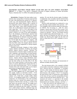

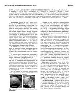


© Copyright 2026