1. Art and Diseño

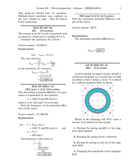
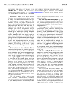
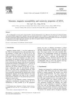
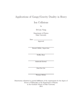
46th Lunar and Planetary Science Conference (2015)
1977.pdf
Depth Estimates and Its Implications from Second Moving Average Residual Magnetic Anomalies on Mars.
K. S. Essa1 and G. Kletetschka2,3,4, 1Geophysics Department, Faculty of Science, Cairo University, 12613 Giza,
Egypt. E-mail: [email protected], 2Institute of Geology, Academy of Science of the Czech Republic, v.v.i., Prague,
Czech Republic, 3Faculty of Science, Charles University in Prague, Czech Republic, 4LBNL, Nuclear Science,
Berkeley, CA, USA. E-mail: [email protected].
Introduction: Mars Global Surveyor mission
obtained detailed magnetic data set of Mars from 400
km satellite altitude, launched in 1996 . Many contrasting magnetic anomalies have been identified [1, 2]
but consensus about the source depth remains unclear.
The variations of magnetic anomalies are greater in
magnitude than the anomalies on Earth [3, 4]. The part
of the southern hemisphere of the Martian crust is
strongly magnetized, as indicated by large intensities of
respective magnetic anomalies, while the northern
hemisphere has lower magnetic signatures suggesting
either lower magnetizations or deeper location of magnetic sources in respect to satellite altitude 400 km.
Variation in magnetization of the source can be due to
several reasons [5, 6].
The formation of the strong crustal magnetic
sources on Mars can be divided into several categories:
the first depends on hydrothermal alteration of preexisting crustal materials to produce efficient remanent
magnetization carriers over large depth ranges [7]. The
second category employs water rich fluids that precipitate iron rich carbonates for which we have evidence in
Martian meteorites [8]. The third category considers
highly magnetic intrusions, which are rich in iron [9].
Possible remanence carriers on Mars include magnetite, hematite, and pyrrhotite [10].
The aim of the present study is using Mars total magnetic data (Fig. 1) to estimate the depth of the
buried sources using a second moving average (SMA)
method [11]. Twelve profiles were chosen across major
magnetic areas. Each profile was subjected to the SMA
separation technique. SMA residual anomalies were
obtained from magnetic data using filters of successive
spacing. The depth estimate is monitored by a standard
deviation of the SMA determined depths for three
shape factor values (q) that include dike, cylinder, and
sphere. The depth estimates for sources of the specific
anomalies, along with related estimate of its standard
deviation, are considered to be a new criterion for determining the depth and shape of the buried magnetic
sources on Mars.
Fig. 1. A total intensity global magnetic map of Mars
obtained from 400 km altitude with profles across major magnetic anomalies [3].
The method: The inversion technique depends on the magnetic anomaly T [nT] produced by
most common three shapes (q= 2.5 for sphere, 2 for
cylinder along the profile, 1 for vertical dike) of geologic magnetically contrasting structures and can be
represented by the following equation [12]
T ( xi , z,  , q) KW ( xi , z,  , q) , i  1,2,3,...N
(1)
The numerical SMA residual magnetic anomaly R2(xi, z, θ, q, s) is given [nT] by equation:
6T (xi )  4T (xi  s)  4T (xi  s)  T (xi  2s)  T (xi  2s)
(2)
.
4
where s = 1, 2, 3, . . . spacing units is the window
length in kilometers.
Using equation (2), and substituting for the
following values at xi = 0, xi = s, and xi = -s, respectively, leads to the following nonlinear equation in z [11]
R2 (xi ) 
1
 
 2r  2q
 az2r  4bs2   5 az2r  bs2   az2r  4bs2   az2r  9bs2  
   az2r  bs2 
3z 2r  2q 

 









z  F





 
q
q
q
q
q
4
  a s2  z 2 
4a 4s2  z 2   4a s2  z 2  a 4s2  z 2  4a 9s2  z 2  


 





 
  
(3)
The equation (3) can be solved using the iterative fixed-point method [13]. The iteration form of
equation (3) is given as
z f  f (z j )
(4)
where zj is the initial depth and zf is the revised depth.
zf is be used as the zj for next iteration.
46th Lunar and Planetary Science Conference (2015)
Discussion of the results: We tested the application and stability of this method on twelve magnetic anomalies, P1, P2, P3, … and P12, each of them
containing 4 crossing profiles (a, b, c, d in Fig. 1). The
location of these particular profiles was chosen in places where the data set contains significant isolated magnetic anomaly, which appear on this total intensity
magnetic map (Fig. 1). Each profile was subject to inversion techniques yielding the depth (z) and the shape
of the buried structure (q). The inversion results of
twelve sets of profiles (P1, P2, P3, … and P12) suggest
that the sources of Martian crustal magnetic anomalies
consist primarily of dikes rich in magnetic minerals
suggesting that the sources may have undergone stratification/lamination during the crustal differentiation of
Mars. This supports convection mechanisms for releasing the heat from the early forming planet [14].
Depth estimates of the magnetic sources (Fig
2.) indicates that the half of the southern hemisphere
starting from southern part of Tharis volcanic province
have much shallower sources (120 – 260 km) than the
opposing half containing Hellas impact structure. The
deepest sources are near hight sourthern latitudes
north-east from the Prometheus impact basin.
Fig. 2. The inversion depth map of the twelve magnetic
anomalies.
Summary remarks: The relatively simple
technique for practicalsepth estimates has been illustrated on twelve magnetic anomaly profiles with various geological settings on Mars. The estimated inverse
parameters based on the real data contrast the view that
the Martian anomalies cannot be deeper than 50 km
[15-17]. Our analysis as well as other even more simple techniques [11] suggest sources exceeding 100 km
depth. The results produced in this analysis indicate
that magnetic anomalies on Mars are generated by dike
shape bodies at depth between 100 and 500 km whose
depth consistently increase towards the region north
east of the Prometheus impact basin and is suddenly
shallowed under the Tharsis volcanic province.
1977.pdf
References:
[1] Acuna M. H. et al. (2001) J. Geophys. Res.Planets, 106(E10), 23403-23417.
[2] Connerney J. E. P.
et al. (1999) Science,
284(5415), 794-798.
[3] Connerney J. E. P. et al. (2001) Geophys. Res.
Lett., 28(21), 4015-4018.
[4] Purucker M. et al. (2000) Geophys. Res. Lett.,
27(16), 2449-2452.
[5] Kletetschka G. et al. (2000) Meteoritics &
Planetary Science, 35(5), 895-899.
[6] Kletetschka G. et al. (2005) Physics of the Earth
and Planetary Interiors, 148(2-4), 149-156.
[7] Quesnel Y. et al. (2009) Earth Planet. Sci. Lett.,
277(1-2), 184-193.
[8] Scott E. R. D. and Fuller M. (2004) Earth Planet.
Sci. Lett., 220(1-2), 83-90.
[9] Arkani-Hamed J. (2005) J. Geophys. Res.-Planets,
110(E12).
[10] Kletetschka G. et al. (2004) Meteoritics &
Planetary Science, 39(11), 1839-1848.
[11] Abdelrahman, E. M. et al. (2004) Journal of King
Abdulaziz University: Earth Sci., 15, 181-196.
[12] Abdelrahman E. S. M. and Essa K. S. (2005)
Geophysics, 70(3), L23-L30.
[13] Mustoe L. R. and Barry M. D. J. (1998),
Mathematics in Engineering and Science, Wiley, New
York.
[14] Kletetschka G. et al. (2009) Meteoritics &
Planetary Science, 44(1), 131-140.
[15] Dunlop D. J. and Arkani-Hamed J. (2005) J.
Geophys. Res.-Planets, 110(E12), 1-11.
[16] Harrison K. P. and Grimm R. E. (2002) J.
Geophys. Res.-Planets, 107(E5).
[17] Langlais B. and Thebault E. (2011) Icarus,
212(2), 568-578.