
Soil Management - Indira Gandhi Agricultural University
IGKV/Pub./2014/15 Soil Management Practical Manual Based on course No. ACP 426 credit 4 (1+3) being taught to under graduate students of agriculture faculty of Indira Gandhi Krishi Vishwavidyalaya, Raipur (C.G.) Authors Dr. Girijesh Kumar Sharma Dr. Dushyant SinghThakur Shri Jawahar Lal Chaudhary Indira Gandhi Krishi Vishwavidyalaya Shaheed Gundadhoor College of Agriculture & Research Station Kumhrawand, Jagdalpur – 494005 (C.G.) 2014 Patron & Inspiration Dr. S. K. Patil, Hon'ble Vice Chancellor Indira Gandhi Krishi Vishwavidyalaya, Raipur (C.G.) Guidance: Dr. S. C. Mukharjee, Dean S.G. College of Agriculture and Research Station, Jagdalpur (C.G.) Compiled and Edited: Dr. Girijesh Kumar Sharma, Scientist (Soil Science and Agri. Chemistry) Dr. Dushyant SinghThakur, Chief Scientist (Soil Science and Agri. Chemistry) Shri Jawahar Lal Chaudhary, Senior Scientist (Agricultural Meteorology) All India Coordinated Research Project for Dryland Agriculture, S.G. College of Agriculture and Research Station, Jagdalpur (C.G.) Published by Dean, S.G. College of Agriculture and Research Station, Jagdalpur Citation : Sharma, G.K. Thakur, D.S. and Chaudhary, J.L. 2014. Soil management Practical manual Published by IGKV Raipur vide Publication No. IGKV/Pub./2014/15 Page 34. Contents S. No. Exercise Page 1. Determination of soil pH 01 2. Determination of soil Bulk Density 02 3 Determination of soil texture by International pipette method 03 4. Determination of soil electrical conductivity (EC) 06 5. Determination of soil cation exchange capacity (CEC) 08 6. Determination of soil organic carbon 10 7. Determination of soil microbial biomass C 11 8. Determination of soil microbial biomass N 13 9. Determination of Dehydrogenase activity 15 10. Determination of soil Exchangeable Sodium Percentage (ESP) 16 11. Determination of soil Sodium Adsorption Ratio (SAR) 19 12. Determination of available cations and anions present in soil 20 13. Determination of Lime Requirement (LR) 21 . 14. Determination of Gypsum Requirement (GR) 22 15. Visit to problematic areas to acquaint with production constraints 23 16. Study of a soil profile 24 17. Soil sample collection 25 18. Irrigation water quality assessment and its effect on soil 27 19. Diagnostic symptoms of nutrient deficiency and toxicity of common crops 28 20. Formulation of soil test based fertilizer doses with IPNS for targeted crop yields 33 21. References 34 Practical Manual Exercise No. 1 DETERMINATION OF SOIL pH Objectives: 1. To know whether the soil is acidic, neutral or alkaline in nature 2. To know the degree of acidity or alkalinity of soil 3. To know the potency of toxic substances present in soil 4. To know the microbial environment of the soil which further indicates the mineralization of organic matter and immobilization of available plant nutrients 5. To know the physical condition of soil like soil structure and permeability of soil. Principle: The degree of acidity or alkalinity can be represented by its intensity. The intensity is represented by the amount of ions (g ions l–1). The substances that give H+ ions in its aqueous solution are called acids where as those who – + – give OH ions are called bases. In an aqueous solution, the product of H and OH ions is constant at constant –14 temperature (i.e. 10 ). Therefore, the intensity of acidity or alkalinity of a solution can be determined on the basis of + + its H ions concentration. The pH is defined as the negative logarithm to the base 10 of H ions activity (concentration) expressed in g ions (moles) l–1 of solution and expressed by the equation: pH= –log10 [H+] or pH= log10 1/[H+]. This concentration is practically measured by the electric potential produced between a glass and reference electrode. Apparatus and Reagents: 1. pH meter with glass and reference electrode 2. beaker 3. buffer solutions( 4,7 and 9.2 pH) 4. Distilled water 5. Electronic balance, glass rods Procedure: 1. Weigh 20 g soil sample in a beaker. 2. Add 50 ml distilled water to it, shake well and retain for 30 minutes. 3. Switch on the pH meter and let it be warm up for 10-15 minute. 4. Calibrate the pH meter by dipping the electrodes in buffer solutions. 5. Dip the electrodes in sample solution and note the reading. Soil pH Rating: < 5 pH 5-6.5 pH 6.5-7.5 pH 7.5-8.5 pH > 8.5 pH — — — — — Strongly acidic Moderately to slightly acidic Neutral Moderately alkaline Strongly alkaline Result: The pH of the given soil sample is……and soil is categorized as acidic/alkaline/neutral. 01 Practical Manual Exercise No. 2 DETERMINATION OF SOIL BULK DENSITY Objectives: 1. 2. 3. 4. 5. To calculate the pore space of a soil when particle density is known To convert the values of mass wetness to volume wetness To know the degree of compactness of a soil and the ease of soil aeration To give some idea about the condition for growth and development of soil micro organisms To estimate the weight of a definite volume soil such as weight of a furrow slice soil of one hectare land Principle: The bulk density or apparent density of soil may be defined as the mass of oven dry soil per unit volume of soil in its natural undisturbed condition. Bulk density (Db) = weight of oven dry soil / bulk volume of soil gram per cm3 or Mega gram per m3 Numerous procedures have been developed for determining bulk density. We will learn the core method for bulk density . The core method is quick and relatively easy method. Apparatus required: Balance, aluminum moisture box, hot air oven, desiccator, cylindrical core sampler (thin walled brass tube), knife, plastic tray, marker etc. Procedure: 1. On a flat soil surface, core sampler is hammered or pressed to insert it into the soil. 2. The core sampler is taken out of the soil. 3. The content of the sampler is transferred completely in a previously weighted moisture box. 4. Dry the contents in an oven at 105ºC for 10-18 hours to get a constant weight. 5. Cool in a desiccator and record the oven-dry weight of the soil core. 6. Calculate the volume of the core sampler. (Volume = r2h) 7. Calculate the bulk density of your soil and record the value (Bulk density = weight of oven dry soil / bulk volume of soil) Observations to be recorded: a. Internal radius of cylindrical core sampler(r) = …………………cm b. Length of core sample(h) = ………………….cm c. Wt. of empty moisture box =…………………...gm d. Wt. of oven dry soil + moisture box =…………………...gm Calculations: A. Volume of cylindrical soil core = r2h = …………cm3 B. Weight of oven dry soil (d-c) = ………….gm C. Bulk density (B/A) = …………. g cm–3 or Mg m–3 Results: The soil bulk density of given field is ................................ gcm–3 Discussion: 1. What is the relationship between soil porosity and bulk density? 2. How do slight changes in bulk density impact soil porosity. 3. Calculate how many kg of the soil is in a hectare plow layer. The plow depth is 15 cm and the area of a hectare is 10000 m2. Express the Db in gcm–3. The density of water is 1.0 g cm–3. 4. How do changes in soil texture impact bulk density and porosity? 5. How does compaction impact bulk density and porosity? EXPECTED VALUES Approximate range of expected bulk density values: 1.0gcm–3 for clay soils to 1.8gcm–3 for sandy or compacted soils. 02 Practical Manual Exercise No. 3 DETERMINATION OF SOIL TEXTURE BY INTERNATIONAL PIPETTE METHOD Objectives: 1. To know the suitability of soils for the production of different crop plants as soil texture has great effect on plant growth and all kinds of soil manipulations influences the retention and transmission of water, soil aeration and the nutrient supplying ability of mineral fraction of soil solid. 2. To classify the soils and to evaluate phenomena such as clay migration, stage of weathering and age of the parent material by the ratio between silt and clay. 3. To study the genesis of soil and to classify them for mapping by the texture of the entire soil profile. 4. To know the suitability of soils for foundation of buildings and for construction of roads. Apparatus Required : Sieves (2.0 and 0.2 mm), 500 mL tall shaped beaker, water bath, rubber tipped glass rod, shaker or stirrer, 1000 mL measuring cylinder with stopper (graduated length is 36 ± 2 cm), filter paper (Whatman no. 44), buckner funnel, vacuum pump, special plunger for mixing, stop watch, glass marking pen, specially made mechanical analysis pipette. Reagents Required : Hydrogen peroxide (30%), sodium sulphide, oxalic acid, hydrochloric acid (2 N), Sodium hydroxide (1 N) or calgon solution (5%) [ Calgon is a commercial preparation of mixing 40 gm sodium hexametaphosphate with 10 gm sodium carbonate. This 50 gm calgon when dissolved in water and diluted to a volume of 1 liter gives 5 % calgon solution whose pH should be 8.3]. Principal: The main principal of this method is to determine the concentration of soil particles at a given depth as a function of time. The concentration of soil particles at depth 'h' and time't' will be the concentration of particles of different diameter having velocity less than h/t. The different size particles will fall through the fluid at different rates. The time't' needed for important soil t= 18h 2 d g (s - w) separates to fall through a height 'h' is obtained from the Stoke's equation as state below: where t is the time in seconds for a particle to fall in h cm, is the viscosity of the fluid in poise, d is the diameter of the particles in cm, g is acceleration due to gravity in cm/sec2, s is the density of soil particles in gm/cm3 and w is the density of fluid in gm/cm3. Since the viscosity and density of fluid are influenced by temperature, the variations in temperature will cause the changes in rate of fall. So the value of viscosity and density at the prevailing temperature is considered in the calculation. Procedure: Dispersion: 40 g air dry processed (i.e. passed through a 2 mm sieve) loamy soil (25 g for clayey soil and 100 g for sandy soil) is taken in 500 mL tall shaped weighed beaker and about 50 mL water is added to make the soil wet. Then about 50 mL hydrogen peroxide is added to the beaker, its content is swirled for few minutes, the beaker is covered with watch glass and left for some time to proceed the reaction in cool. After that the covered beaker is placed on a hot water bath at a temperature of about 65 to 700C and the content is stirred occasionally with glass rod watching it carefully and removing it from water bath when necessary to prevent frothing over. This process is continued till the reaction completely subsides. In case frothing persists, the process is repeated by adding again 25 to 30 mL of hydrogen peroxide in the beaker and places it on the hot water bath. This process is continued until the whole organic matter is oxidized (i.e. warming produces no further reaction). The beaker is then heated to about 900 to 1000C to remove the excess hydrogen peroxide. 03 Practical Manual In calcareous soils, 25 mL of diluted (2N) hydrochloric acid is added to the peroxide treated soil and left until effervescence ceases. The suspension is then filtered using Whatman No. 44 filter paper on a buckner funnel connected with a vacuum pump and washed repeatedly with distilled water till it is acid free (when the soil is treated with hydrochloric acid, chloride free is tested with silver nitrate solution). In red and laterite soils 100 mL of water and a pinch (0.5 to 2 gm each) of oxalic acid and sodium sulphide are added to the beaker before hydrogen peroxide treatment and the beaker is placed on hot water bath for about an hour. The content of the beaker is filtered through a Buchner funnel under vacuum using a Whatman No. 44 filter paper. The soil is repeatedly washed with distilled water till it is free from soluble salts or soluble ions and chloride ions. The soil from the filter paper is then transferred to the same weighed 500 ml beaker with a jet of distilled water and rubber tipped glass rod. Care should be taken so that all fine materials from the surface of the filter paper are removed and minimum quantity of water is used. The content of the beaker is gently evaporated to dryness first on a hot plate and then in an oven at 1050C for about 16 hours. After cooling in a desicator the beaker and the content is weighed and the weight is recorded for subsequent calculation. 25 ml of sodium hydroxide or 20 ml of calgon solution is added to the dry soil and left for over night. The mixture is transferred with water to the cup of a high speed stirrer and the volume is made up to about 400 ml. The mixture is stirred for 5 to 10 minutes. The stirred blades are washed down as they are removed from the suspension. Fractionation: Separation of course sand: The dispersed soil suspension is transferred to a 1 liter cylinder by pouring it through standard sieve having 0.2 mm diameter which retains coarse sand. The material on the sieve is washed with distilled water along with rubbing gently with rubber tip glass road so that no particles are retained on the sieve. The course sand fraction is transferred to a weighed small container (No.1) by brushing off the sieve surface carefully and the material is dried at 1050C in an oven for about five hours. The container along with sand fraction is cooled in a desicator and weighed. Separation of silt and clay: The volume of the suspension in the cylinder is made up to one liter by adding distilled water. The cylinder is placed in a temperature controlled chamber. A mark is given on the cylinder at 10 cm depth from the surface of the suspension. The temperature of the suspension is measured and proper of sedimentation for silt plus clay and for clay corresponding to that temperature is noted from table. The content of the cylinder is mixed thoroughly for one minute with the help of a plunger or moved up and down for about 20 times in one minute after putting the stopper. The plunger or stopper is removed and is waited until the swirling motion of the particles has just stopped and steady setting under gravity has just standard. The stop watch is started. Table: sedimentation times for soil particles settling through a depth of 10 cm in water (particle density 2.6 gm/cm3) Temperature (OC) Settling time with indicated particle diameter 2 microns Hour 5 microns Minute Hour 20 microns Minute Hour Minute 20 8 0 1 17 4 48 21 7 49 1 15 4 41 22 7 38 1 13 4 35 23 7 27 1 11 4 28 24 7 17 1 10 4 22 25 7 7 1 8 4 16 26 6 57 1 7 4 10 27 6 48 1 5 4 4 28 6 39 1 4 4 0 29 6 31 1 3 3 55 30 6 22 1 1 3 49 31 6 14 1 0 3 44 04 Practical Manual The specially made mechanical analysis pipette is gently lowered into the cylinder up to a depth of 10 cm from the surface of the suspension about 10 second before the sampling time and 10 ml of suspension (20 ml for light textured soils) is carefully withdrawn just after the desired time. The content of the pipette is taken into a weighed container (No. 2 for silt plus clay and No. 3 for clay) and the pipette is washed twice with water and the washing is added to the dish. The content of the dish is dried in an oven at 1050 C for about 16 hours cooled in a desiccator and weighed. The dry weight of the sample plus dish is recorded. Percent fine sand may be determined by subtracting the sum of course sand, silt and clay from 100. Observations: a. Weight of the soil taken =………………………………..gm b. Weight of container No. 1 =……………………………..gm c. Weight of container No. 1 plus oven dry soil after removal of cementing agents and salts=……………………………..gm d. Weight of container No. 2 =……………………………..gm e. Weight of container No. 2 plus dry course sand fraction =……………………gm f. Volume of suspension taken for analysis =……………………….ml g. Weight of container No. 3 =……………………………..gm h. Weight of container No. 3 plus dry silt plus clay =……………………………..gm i. Weight of container No. 4 =……………………………..gm j. Weight of container No. 4 plus dry clay =……………………………..gm Calculations: I. Oven dry weight of the soil after removal of cementing agents and salts (c-b) =……gm II. Weight of course sand (e-d) =…………………..gm III. Percent course sand (II/I) x 100 =……………….% IV. Weight of silt plus clay (h-g) =………………….gm V. Percent silt plus clay (IV/I) x (1000/f) x 100 =………………% VI. Weight of clay (j-i) = …………………….gm VII.Percent clay (VI/I) x (1000/f) x 100 =………………% VIII. Percent silt (V-VII) =…………………………………% IX. Percent fine sand [100 - (111 + V)] =……………………% Result: the percent course sand, fine sand, silt, and clay are………………………………… respectively. By reading these values in textural triangle the texture of the given soil sample is……………………. 05 Practical Manual Exercise No. 4 SOIL ELECTRICAL CONDUCTIVITY(EC) Objectives : To determine the salt content of the soil Principle : The electrical conductivity (EC) is a measure of the ionic transport in a solution between the anode and cathode. This means, the EC is normally considered to be a measurement of the dissolved salts in a solution. Like a metallic conductor, they obey Ohm's law. Since the EC depends on the number of ions in the solution, it is important to know the soil/water ratio used. The EC of a soil is conventionally based on the measurement of the EC in the soil solution extract from a saturated soil paste, as it has been found that the ratio of the soil solution in saturated soil paste is approximately two-three times higher than that at field capacity. As the determination of EC of soil solution from a saturated soil paste is cumbersome and demands 400-500 g soil sample for the determination, a less complex method is normally used. Generally a 1:2 soil/water suspension is used. The soils having pH value more than 8.0-8.5 may have the following special features: Presence of excessive amounts of soluble salts. Presence of excessive amounts of sodium on the exchange complex. The chemical properties of salt affected soils are summarized in Table. TABLE : Chemical characteristics of saline, non-saline sodic and saline sodic soils Soil EC (dS/m) ESP pH Saline >4.0 <15 <8.5 Sodic (non-saline) <4.0 >15 >8.5 Saline Sodic >4.0 >15 <8.5 Source: Richards, 1954 Such soils are generally not considered suitable for growing most of the crops unless treated with suitable amendment materials. However, there are salt tolerant crops which could be grown on these soils. To determine the quality of these soils, the following estimations are required: pH (as described before) Salt content or electrical conductivity Exchangeable sodium or gypsum requirement 06 Practical Manual Apparatus : EC meter Beakers (25 ml), erlenmeyer flasks (250 ml) and pipettes Filter paper Reagent : 0.01M Potassium chloride solution: Dry a small quantity of AR grade potassium chloride at 600 C for two hours. Weight 0.7456 g of it and dissolve in freshly prepared distilled water and make the volume to one litre. This –3 0 solution gives an electrical conductivity of 1411.8x10 i.e. 1.412 mS/cm at 25 C. For best result, select a conductivity standard (KCl solution) close to the sample value. Procedure : 1. Take 40 g soil into 250 ml Erlenmeyer flask, add 80 ml of distilled water, stopper the flask and shake on reciprocating shaker for one hour. Filter through Whatman No.1 filter paper. The filtrate is ready for measurement of conductivity. 2. Wash the conductivity electrode with distilled water and rinse with standard KCl solution. 3. Pour some KCl solution into a 25 ml beaker and dip the electrode in the solution. Adjust the conductivity meter to read 1.412 mS/cm, corrected to 250 C. 4. Wash the electrode and dip it in the soil extract. 5. Record the digital display corrected to 250 C. The reading in mS/cm of electrical conductivity is a measure of the soluble salt content in the extract, and an indication of salinity status of this soil (Table). The conductivity can also be expressed as mmhos/cm. TABLE : General interpretation of EC values S.No. Soil EC(mS/cm) Total salt content (%) Crop reaction Salinity effect negligible, except for more sensitive crops 1. Salt free 0-2 <0.15 2. Slightly saline 4-8 0.15-0.35 Yield of many crops restricted 3. Moderately saline 8-15 0.35-0.65 Only tolerant crops yield satisfactorily 4. Highly saline >15 >0.65 07 Only very tolerant crops yield satisfactorily Practical Manual Exercise No. 5 DETERMINATION OF SOIL CATION EXCHANGE CAPACITY (CEC) Objectives: 1. To evaluate the fertility status of soil from the knowledge of CEC together with exchangeable bases. 2. To evaluate the capacity of soil to retain the maximum amount of the important nutrient cations. 3. To find out the maximum doses of water soluble cationic fertilizer to be applied at a time so that they are not subjected to appreciable loss by leaching during the period of excessive rainfall. 4. To calculate the amount of lime in acid soils and amount of gypsum in alkali soil from the knowledge of CEC along with exchangeable bases. Materials required: Apparatus: Balance, conical flasks, Buchner funnel, Distillation unit, pipette, filter paper (ordinary and Whatman No. 42). Reagents: 1. Neutral normal ammonium acetate solution: dissolve 77 gm of ammonium acetate in 100 ml distilled water. The pH of the solution is adjusted to 7.0 by adding either 3N acetic acid or 3N ammonium hydroxide and make up the volume upto 1000 ml. 2. Alcohol (60 %): 520 ml of water is added to absolute alcohol. 3. Other reagents: sulphuric acid (0.1N), sodium hydroxide (0.1N), MgO powder, NH4Cl crystals, methyl red indicator, silver nitrate solution. Principal: The soil complex is saturated with an index cation (usually ammonium ion) by saturating the soil and subsequently leaching it with neutral normal ammonium acetate solution. The cations of the soil are displaced by + ammonium ions and the soil surface is saturated with NH4 ions. The excess ammonia and the displaced cations are + removed by washing with alcohol. The adsorbed NH4 is then determined by steam distillation as ammonia using MgO. The ammonia gas evolved during distillation is absorbed in a known volume of standard acid and the unreacted acid molecules are back titrated with standard alkali. Procedure: 25 gm of soil is transferred to a 500 ml conical flask and 250 ml of neutral normal ammonium acetate solution is added. The contents are occasionally shaken for an hour and kept overnight. The contents are filtered through Whatman No. 42 filter paper receiving the filtrate in a 100 ml measuring flask. The soil is transferred completely on the filter paper and the soil is leached with neutral normal ammonium acetate solution (using about 25 ml at a time) allowing the leachete to drain completely before a fresh aliquot is added. One liter of leachate is collected and this is reserved for determination of individual cations. The residue left on the filter paper is used for determination of the total cation exchange capacity of the soil. 08 Practical Manual A pinch of solid ammonium chloride is added to the soil on the filter paper and the soil is washed with 60 % alcohol to eliminate the excess of ammonium acetate. The washing is continued till the filtrate becomes free of chloride (it is tested with silver nitrate solution). When this is attained the soil is removed from the filter paper into the distillation flask. About 200 ml of water and 0.5 gm of magnesium oxide are added. The flask is stopped and the distilled ammonia is absorbed in to standard 0.1 N sulphuric acid to which a few drops of methyl red is added. The excess acid is back titrated with standard 0.1 N sodium hydroxide. One blank test is conducted with the same volume of NH4OAc. Observations: a. Weight of standard 0.1 N NaOH =………………………………..gm b. Volume of standard 0.1 N NaOH required for sample titration =………ml c. Volume of standard 0.1 N NaOH required for blank titration =………ml d. Actual strength of 0.1 N NaOH =…………………..N Calculations: e. meq. of NaOH used for sample titration (bxd) =……… meq. f. meq. of NaOH used for blank titration (cxd) =……… meq. g. meq. of H2SO4 consumed for ammonia absorption (e-f) = ……… meq. h. CEC of the soil (gx100/a) =…………………. meq/100 gm =……………………….c mol (p+)/kg Results: The CEC of the given soil sample is…………… Interpretation: The results are interpreted by using the following rating chart: Rating CEC (meq/100 gm or c mol (p+)/kg of soil Low < 10 Medium 10-25 High 25-45 Very high > 45 09 Practical Manual Exercise No. 6 ORGANIC CARBON/ORGANIC MATTER (Walkley and Black, 1934) Organic matter estimation in the soil can be done by different methods. Loss of weight on ignition can be used as a direct measure of the organic matter contained in the soil. It can also be expressed as the content of organic carbon in the soil. It is generally assumed that on an average organic matter contains about 58% organic carbon. Organic matter/organic carbon can also be estimated by volumetric and colorimetric methods. However, the use of potassium dichromate (K2Cr2O7) involved in these estimations is considered as a limitation because of its hazardous nature. Soil organic matter content can be used as an index of N availability (potential of a soil to supply N to plants) because the content of N in soil organic matter is relatively constant. Apparatus: Conical flask - 500 ml, Pipettes - 2, 10 and 20 ml, Burette - 50 ml Reagents: Phosphoric acid - 85% Sodium fluoride solution - 2% Sulphuric acid - 96 % containing 1.25% Ag2SO4 Standard 0.1667M K2Cr2O7: Dissolve 49.04 g of K2Cr2O7 in water and dilute to 1 litre Standard 0.5M FeSO4 solution: Dissolve 140 g Ferrous Sulphate in 800 ml water, add 20 ml concentrated H2SO4 and make up the volume to 1 litre Diphenylamine indicator: Dissolve 0.5 g reagent grade diphenylamine in 20 ml water and 100 ml concentrated H2SO4. Procedure: 1. Weigh 1.0 g of the prepared soil sample in 500 ml conical flask. 2. Add 10 ml of 0.1667M K2Cr2O7 solution and 20 ml concentrated H2SO4 containing Ag2SO4. 3. Mix thoroughly and allow the reaction to complete for 30 minutes. 4. Dilute the reaction mixture with 200 ml water and 10 ml H3PO4. 5. Add 10 ml of NaF solution and 2 ml of diphenylamine indicator. 6. Titrate the solution with standard 0.5M FeSO4 solution to a brilliant green colour. 7. A blank without sample is run simultaneously. Calculation: Percent organic Carbon (X) = 10 (S -T) × 0.003 100 × S Wt. of soil Since one gram of soil is used, this equation simplifies to: 3(S – T) S Where, S = ml FeSO4 solution required for blank , T = ml FeSO4 solution required for soil sample, 3 = Eq W of C (weight of C is 12, valency is 4, hence Eq W is 12 ÷ 4 = 3.0), 0.003 = weight of C (1 000 ml 0.1667M K2Cr2O7 = 3 g C. Thus, 1 ml 0.1667M K2Cr2O7 = 0.003 g C) Organic Carbon recovery is estimated to be about 77%. Therefore, actual amount of Organic carbon (Y) will be: Or Percentage value of organic carbon × 1.3 Percent value of organic carbon obtained × Percent Organic matter = Y x 1.724 (organic matter contains 58 % organic carbon, hence 100/58 = 1.724) 100 77 Note: Published organic C to total organic matter conversion factor for surface soils vary from 1.724 to 2.0. A value of 1.724 is commonly used, although whenever possible the appropriate factor be determined experimentally for each type of soil. 10 Practical Manual Exercise No. 7 DETERMINATION OF SOIL MICROBIAL BIOMASS C Microbial biomass C is determined by the fumigation/incubation technique in which a fresh soil sample is subjected to chloroform fumigation, which causes cell walls to lyse and denature, the cellular contents are extractable in 0.5 M K2SO4. This is not a measure of soil microbial activity because no differentiation is made between quiescent and active organisms, or between different classes of microorganisms. Care must be exercised when comparing soils from different locations as microbial biomass fluctuates greatly within a single soil in response to litter inputs, moisture availability and temperature. If different agricultural soils are being compared at a single time, the fresh soils should be at or near moisture holding capacity. If soils from different ecosystems are being compared, samples should be collected toward the middle of the wet and dry seasons. The following procedure is based on that of Anderson and Ingram (1993), and taken from Okalebo et al. (1993). Apparatus: Block-digester with calibrated digestion tubes, distillation unit, Automatic titrator connected to a pH meter, Vortex tube stirrer, desiccator, mechanical shaker, orbital, standard laboratory glassware: Beakers, volumetric flask, pipettes, and funnels. Reagents: A. Chloroform Solution (CHCl3), alcohol-free: Wash chloroform with 5% concentrated sulfuric acid in a separation funnel, separate the acid and then rinse repeatedly (8 - 12 times) in DI water. Store in a dark bottle. B. Potassium Sulfate Solution (K2SO4), 0.5 M :Dissolve 87.13 g potassium sulfate in DI water, and bring to 1-L volume with DI water. C. Copper Sulfate Solution (CuSO4.5H2O), 0.2 M: Dissolve 49.94 g copper sulfate in DI water, and bring to 1-L volume with DI water. D. Potassium Dichromate Solution (K2Cr2O7), 0.4 N: Dissolve 19.616 g potassium dichromate in DI water, and bring to 1-L volume with DI water. E. Ferrous Ammonium Sulfate Solution [Fe (NH4)2(SO4)2.6H2O], 0.2 N: Dissolve 78.4 g ferrous ammonium sulfate in DI water, add 5 Ml concentrated sulfuric acid, mix well, and bring to 1-L volume in DI water. F. 1.10-Phenanthroline Indicator: Dissolve 14.85 g 1.10-phenanthroline indicator, and 6.95 g ferrous sulfate (FeSO4.7H2O) in DI water, and bring to 1-L volume in DI water. G. Sulfuric-Orthophosphoric Acid Mixture (H2SO4: H3PO4), 2:1 concentrated: Add 1000 mL concentrated sulfuric acid to 500 mL concentrated orthophosphoric acid. Procedure: 1. Weigh duplicate 30 g fresh soil samples into a 100-mL beaker. Conduct a moisture determination on soil sub-samples so that the results can be expressed on an oven-dry-weight basis. 2. Place the beakers into the two desiccators. Place a 100-mL beaker containing 50 mL chloroform into the center of the desiccator. Adding pumice boiling granules to the chloroform assists in rapid volatilization of the chloroform. The second desiccator contains non-fumigated control samples, which apart from fumigation-evacuation are to be handled in the same fashion. Close the lids of the desiccators, paying particular attention that the sealant is uniformly distributed (Fig. 7). 3. Apply vacuum to the fumigated treatment until the chloroform is rapidly boiling. 4. Close the desiccator and store under darkened conditions for 72 hours at room temperature. 5. Evacuate the fumigated treatment using a vacuum pump repeatedly (8 - 12 times). Important: Remember that the chloroform is being trapped by the oil in the vacuum pump; so the oil must be changed more often 11 Practical Manual than normal. Alternatively, chloroform can be trapped by a cooling finger to prevent contamination of the vacuum oil. It is not necessary to evacuate the control desiccator. 6. Open the desiccators, and transfer the fumigated/nonfumigate soil samples to 250-mL Erlenmeyer flasks. Add 100 mL 0.5 M potassium sulfate solution and shake on an orbital shaker for 1 hour. 7. To obtain a clear extract, filter the soil suspensions using Whatman No. 42 filter paper or a centrifuge. Determination of Carbon A. Digestion 1. Pipette 8 mL of the filtrate into a 100-mL calibrated digestion tube, and add 2 mL 0.4 N potassium dichromate solution. 2. Add 0.07 g mercury (II) oxide (HgO), 15 mL (2:1) sulfuric: orthophosphoric acid mixture, and a few pumice boiling granules. 3. Place the tubes rack in the block-digester, increase temperatures setting to 150°C and digest for 30 minutes. 4. Carefully lift the tubes rack out of the block-digester, let tubes cool to room temperature, and transfer the digested sample with 25 mL DI water into a 250-mL Erlenmeyer flask. B. Titration: Add 2 - 3 drops 1.10-phenalthroline indicator, and then titrate with 0.2 N ferrous ammonium sulfate solutions, until the color changes from bluish-green to reddish-brown. CALCULATION: Biomass C (ppm) = (V - B) × N × 0.003 × 100 + Wt × 1000 × 1000 V For Biomass Carbon in soil Microbial Biomass C = (C fumigated - C control) Where: V = Volume of 0.2 N [Fe(NH4 )2 (SO4 )2 .6H2O] titrated for the sample (mL) B = Digested blank titration volume (mL) N = Normality of [Fe (NH4 )2 (SO4 )2 . 6H2O] solution. 0.003= 3 × 10⁻³, where 3 is equivalent weight of C. Wt = Weight of fresh soil (g), V = Aliquot used for soil digest measured (mL) = Weight of water (g) per 30 g fresh soil. 12 Practical Manual Exercise No. 8 DETERMINATION OF SOIL MICROBIAL BIOMASS N Microbial biomass N is determined by the fumigation/incubation technique in which a fresh soil sample is subjected to chloroform fumigation, which causes cell walls to lyse and denature, the cellular contents are extractable in 0.5 M K2SO4. This is not a measure of soil microbial activity because no differentiation is made between quiescent and active organisms, or between different classes of microorganisms. Care must be exercised when comparing soils from different locations as microbial biomass fluctuates greatly within a single soil in response to litter inputs, moisture availability and temperature. If different agricultural soils are being compared at a single time, the fresh soils should be at or near moisture holding capacity. If soils from different ecosystems are being compared, samples should be collected toward the middle of the wet and dry seasons. The following procedure is based on that of Anderson and Ingram (1993), and taken from Okalebo et al. (1993). Apparatus: Block-digester with calibrated digestion tubes, distillation unit, Automatic titrator connected to a pH meter, Vortex tube stirrer, desiccator, mechanical shaker, orbital, standard laboratory glassware: Beakers, volumetric flask, pipettes, and funnels. Reagents: A. Chloroform Solution (CHCl3), alcohol-free Wash chloroform with 5% concentrated sulfuric acid in a separation funnel, separate the acid and then rinse repeatedly (8 - 12 times) in DI water. Store in a dark bottle. B. Potassium Sulfate Solution (K2SO4), 0.5 M Dissolve 87.13 g potassium sulfate in DI water, and bring to 1-L volume with DI water. C. Copper Sulfate Solution (CuSO4.5H2O), 0.2 M Dissolve 49.94 g copper sulfate in DI water, and bring to 1-L volume with DI water. D. Potassium Dichromate Solution (K2Cr2O7), 0.4 N Dissolve 19.616 g potassium dichromate in DI water, and bring to 1-L volume with DI water. E. Ferrous Ammonium Sulfate Solution [Fe (NH4)2(SO4)2.6H2O], 0.2 N Dissolve 78.4 g ferrous ammonium sulfate in DI water, add 5 Ml concentrated sulfuric acid, mix well, and bring to 1-L volume in DI water. F. 1.10-Phenanthroline Indicator Dissolve 14.85 g 1.10-phenanthroline indicator, and 6.95 g ferrous sulfate (FeSO4.7H2O) in DI water, and bring to 1-L volume in DI water. G. Sulfuric-Orthophosphoric Acid Mixture (H2SO4: H3PO4), 2:1 concentrated Add 1000 mL concentrated sulfuric acid to 500 mL concentrated orthophosphoric acid. Procedure: 1. Weigh duplicate 30 g fresh soil samples into a 100-mL beaker. Conduct a moisture determination on soil sub-samples so that the results can be expressed on an oven-dry-weight basis. 2. Place the beakers into the two desiccators. Place a 100-mL beaker containing 50 mL chloroform into the center of the desiccator. Adding pumice boiling granules to the chloroform assists in rapid volatilization of the chloroform. The second desiccator contains non-fumigated control samples, which apart from fumigation-evacuation are to be handled in the same fashion. Close the lids of the desiccators, paying particular attention that the sealant is uniformly distributed (Fig. 7). 13 Practical Manual 3. Apply vacuum to the fumigated treatment until the chloroform is rapidly boiling. 4. Close the desiccator and store under darkened conditions for 72 hours at room temperature. 5. Evacuate the fumigated treatment using a vacuum pump repeatedly (8 - 12 times). Important: Remember that the chloroform is being trapped by the oil in the vacuum pump; so the oil must be changed more often than normal. Alternatively, chloroform can be trapped by a cooling finger to prevent contamination of the vacuum oil. It is not necessary to evacuate the control desiccator. 6. Open the desiccators, and transfer the fumigated/nonfumigate soil samples to 250-mL Erlenmeyer flasks. Add 100 mL 0.5 M potassium sulfate solution and shake on an orbital shaker for 1 hour. 7. To obtain a clear extract, filter the soil suspensions using Whatman No. 42 filter paper or a centrifuge. Determination of Nitrogen A. Digestion 1. Pipette 50 mL of the filtrate into a 250-mL calibrated digestion tube, and add 1 mL 0.2 M copper sulfate solution. 2. Add 10 mL concentrated sulfuric acid, and a few pumice boiling granules. 3. Place the tubes rack in the block-digester and increase the temperature setting to 150°C to remove extra water. 4. Increase the temperature slowly to reach to 380°C, and digest for 3 hours. 5. Carefully lifts the tubes rack out of the block-digester, let tubes cool to room temperature, and bring to volume with DI water. 6. Each batch of samples for digestion should contain at least one blank (no soil), and one EDTA standard (0.1g EDTA accurately weighed to 0.1 mg). B. Distillation Distillate the samples and analyze for N, as described in total-N (50 mL digest, and 15 mL 10 N NaOH). CALCULATIONS For Biomass Nitrogen in soil: 100 + Biomass N (ppm) = (V – B) × N × 14.01 × 250 × Wt Microbial Biomass N = (N fumigated - N control) Where: V = Volume of 0.01 N H2SO4 titrated for the sample (mL) B = Digested blank titration volume (mL), N = Normality of H2 SO4 solution. Wt = Weight of fresh soil (g), V1 = Aliquot of soil digest measured (mL) V2 = Aliquot of distillate measured (mL), 14.01 = Atomic weight of N. = Weight of water (g) per 30 g fresh soil. 14 1000 × V1 V2 Practical Manual Exercise No. 9 DETERMINATION OF DEHYDROGENASE ACTIVITY Biological activity index of a soil is the function of number of organisms present in soil and their physiological efficiency. The rate of respiration can be used as an index of the biological activity of soil as it reflects the physiological efficiency of the organisms. Monitoring of dehydrogenises, which are respiratory enzymes and integral part of all soil organisms, will give a measure of biological activity of soil at a given time. Principle: In respiration, biological oxidations of reduced compounds occurs which is catalysed by dehydrogenases. During this process energy is evolved. The process can be represented as: RH2 + A R + AH2 (2H+ 2e) Where, RH2 represents a reduced compound (hydrogen donor) and 'A' is the electron acceptor, which is oxygen in aerobic organisms. Under anaerobic conditions, compound like 2, 3, 5-triphenyl tetrzolium chloride (TTC) can act as electron acceptor. In the process TPC gets reduced to a pink coloured compound triphenyl formazan (TPF), which can be quantitatively extracted by methanol and measured calorimetrically. TTC + 2H+ 2e– TPF The dehydrogenises can be assayed as rate of formation of TPF from TTC. Higher the biological activity faster will be the formation of TPF. Reagents: 1. 3%2, 3, 5- triphenyl tetrazolium chloride (TTC): Dissolve 3 g of TTC in 100 mL of distilled water. Store in an amber coloured bottle 2. Methanol (AR grade) 3. 1% Glucose solution: Dissolve 1g of glucose in 100 mL of distilled Water. 4. Standard triphenyl formazan TPF: Dissolve 100 mg of TPF in 100 mL Of distilled water. Procedure: 1. Put 1gof representative air-dried soil in an air-tight screw capped test tube 2. Add 0.2 mL of 3% TTC solution in each of the tubes to saturate the soil. 3. Add 0.5 mL of 1% glucose solution in each tube. Gently tap the bottom of the tube to drive out all trapped oxygen. A water seal is formed above the soil. Ensure that no air bubbles are formed. 4. Incubate the tubes at 280 ± 0.5 0C temperature for 24 hours. 5. After incubation add 10 mL of methanol. Shake vigorously and allow to stand for 6 hours. 6. Withdraw clear pink coloured supernatant liquid and read the absorbance at a wavelength of 485 nm (blue filter). 7. Extrapolate TPF formed from the standard curve drawn in the range of 10 to 90 mg TPF mL-1. 8. Express the results at mg TPF formed per hour per g soil. 15 of 15 mL capacity. Practical Manual Exercise No. 10 DETERMINATION OF SOIL ESP Determination of soil ESP Exchangeable sodium in soil varies from a small portion to a large portion of the exchange capacity depending on the sodicity of the soil. Like wise water soluble sodium varies from trace amount to a large amount depending on the salinity level of the soil. The degree of sodicity of a soil is normally assessed by exchangeable sodium percentage or ESP which is defined as follows: ESP= (Exch. Na/CEC) ×100 Both exch. Na and CEC i.e. cation exchange capacity are expressed in c mol (+)/kg of soil or meq/100 gm of soil. The salinity level of soil is assessed by the electrical conductivity of the saturation extract (ECe) of the soil which is expressed in dS/m or m. mhos/cm. A sodic soil contains an exchangeable sodium (ESP>15), a saline soil contains an excess amount of soluble salts (ECe >4 dS/m) and a saline sodic soil contains both salt and sodium in excess amount (ESP > 15, ECe > 4 dS/m). Methods of determination: Exchangeable plus water soluble sodium may be extracted by number of extractants like l.N NH4OAc, BaCl2 buffered at a pH of 7.0 to 8.2 and Na may be determined by Flam photometric determination, Atomic absorption determination and Gravimetric determination. Among these, extraction by NH4 OAc and determination by flame photometer is commonly used procedure for determination of exchangeable plus soluble sodium. Water soluble sodium is determined separately in saturation extract by flame photometer. The exchangble sodium is then determined by subtracting the results of water soluble Na from the results obtained for exchangeable plus water soluble sodium. Principle: In this method water soluble and the exchangeable sodium of the soil is extracted by shaking the soil with neutral normal ammonium acetate in 1:5 soil: solution ratio. During equilibrium, ammonium ions exchange with the exchangeable sodium ions along with other exchangeable camions. After equilibrium the suspension is filtered through whatman no.l filter paper. The sodium content of the filtrate is determined with a flame photometer. The reaction is stated below: colloid colloid K Ca + CH3COONH4 NH4 + CH3COOR NH4 NH4 mg NH4 H NH4 Where R means exchangeable cat ions like Na, Ca, Mg, Na etc. Since ammonium acetate extracts both exchangeable and soluble sodium, water soluble sodium of saturation extract is determined by flame photometer and exchangeable sodium content is determined by subtracting the amount found in water soluble sodium from the amount found in NH4OAc extracted sodium. Materials Required: (A) Equipments and other materials: Balance, flame photometer, pH meter. Conical flask, funnels, beakers, pipette, volumetric flask, Whatman no.l paper, spatula, Buchner, suction flask, vacuum pump. (B) Reagents: (1) Normal neutral ammonium acetate solution: 77.09 gm of ammonium acetate is dissolved in water and the volume is made up to one liter. The solution is tested with a pH meter. If not neutral, either ammonium hydroxide or acetic acid is added to adjusted the solution pH to 7.0. 16 Practical Manual (2) Standard sodium solution: (a) Stock solution: 2.542 gm of pure AR grade NaCl (dried at 1100C for 1 hour) is dissolved in distilled water and the volume is made up to one liter. This solution contains 1000 ppm Na. It is treated as stock solution of Na. (b) 100 ppm standard Na: It is prepared by diluting 100 ml of 1000 ppm stock solution to one liter with the extracting solution (neutral normal ammonium acetate). Preparation of standard curve: 0, 5,10,15,20 and 25 ml of 100 ppm solution is taken into 100 ml volumetric flasks and the volume is brought up to the mark with extracting solution (i.e. neutral normal ammonium acetate). The solutions contain 0, 5,10,15,20 and 25 ppm Na respectively. After inserting the Na filter and regulating the appropriate gas air pressure, the flame photometer is set up at 0 for blank (NH4 OAc) and at 100 for 25 ppm of Na solution alternatively till both values are obtained without any adjustment, then working standard solutions are atomized intermittently and the meter readings are recorded. These meter readings are plotted against the sodium contents the points are connected with a straight line. Procedure: 5 gm of soil sample is taken in a 150 ml conical flask and 25 ml of the ammonium acetate extract ant is added to it. The contents of the flask are shaken for five minutes and the suspension is filtered through Whatman no.1 filter paper. The filtrate is atomized in the flame photometer in which 0 and 100 have been set with blank and 40 ppm Na solutions respectively and the reading is noted. The sodium (Na) content of the filtrate is determined from the standard curve and the Na content is calculated. This is exchangeable plus soluble sodium. The soluble sodium is determined from saturation extract. A saturated soil paste is prepared using 100 to 150 gm soil by adding water to the soil and stirring with spatula. The saturated soil paste is transferred on a Whatman No. 42 filter paper placed in a Buchner funnel fitted on a suction flask which in turn is connected with a vacuum pump. The vacuum extraction is terminated when air begging to pass through filter paper. If the filtrate is turbid, it is refiltered. The clear extract is atomized in the Flame photometer to determiner soluble Na. Observation and calculations: A. For soluble & exchangeable sodium: (a) Weight of the soil = 5 gm (b) Volume of the neutral N NH4 OAc = 25 ml (c) Let the readings of the flame photometer for the test solution = X= (d) Let the concentration at X readings 17 Practical Manual read from the standard curve = Y= ppm (e) Dilution factor = 25/5 = 5 times. (f) Soluble plus exchangeable Na in soil =d×5= ppm (g) Soluble plus exchangeable Na for 15 cm soil depth = f × 2.24 = kg/ha B. For soluble sodium: (h) Weight of the soil = 150 gm (i) Volume of water = ml (j) Let the reading of the flame Photometer for the test solution =X= (k) Let the concentration at X reading Read from the standard curve =Y= (l) Dilution factor = i/h ppm = (m) Soluble sodium in soil = k × l times = ppm (n) Soluble Na for 15 cm soil Depth = m × 2.24 = kg/ha (o) Exchangeable sodium for 15 cm Soil depth = g - n = kg/ha (p) Exchangeable sodium in mg/100 gm soil = (o × 106)/(2.24 × 106 10)= o/(2.24×10) = mg/100gm soil (q) Exchangeable sodium of soil In meq/100 gm soil = p/23 = mg/100gm soil (r) If CEC of soil is z meq/100 gm soil Then ESP = (q/z) × 100 = . The ESP and SAR are calculated as follows: A sodic soil contain ESP > 15 ESP = Exchangeable sodium [cmol (+)/kg] Cation exchange capacity [cmol (+)/kg] × 100 Where [Na+], [Ca2+] and [Mg2+] are the concentrations in c mol (+)/kg of the sodium, calcium and magnesium ions in the soil + SAR = [Na ] 2+ 2+ 0.5([ca ] + [Mg ]) solution. 18 Practical Manual Exercise No. 11 DETERMINATION OF SODIUM ABSORPTION RATIO (SAR) Objective : This exercise measures the three species –Na, Ca & Mg – require to determine the sodium absorption ratio (SAR) for soil. Reagents : 1. Atomic Absorption Spectrometer (AAS). 2. Air-dried soil. 3. 1000mg/L Na, Ca & Mg standards. Principal : The SAR may be calculated as follows : + [Na ] SAR = 2+ 2+ 0.5([ca ] + [Mg ]) + 2+ 2+ Where, [Na ], [Ca ] and [Mg ] are the concentrations in c mol (+)/ kg of the sodium, calcium and magnesium ions in the soil solution. Procedure : Sample Preperation : Weigh approximately 250g of air dried soil into each of two beakers. Add deinonised water with stirring until the soil becomes a paste, with no free water being present. Leave the sample to stand for 2 hours (during this time you can prepare your standards). Transfer the soil paste to a suction filter and draw off any water. Filler by Millepore filtration. Transfer the filtrate to a flask for determination of elemental content by AAS. Standard preparation : Devise a scheme for the preparation of mixed standards for Na, Ca and Mg, in the concentrations of 5, 20 and 50mg/L for use in the AAS. This means there will be only three standards with those concentrations of the three analytes. Prepare standards as per step above. AAS analysis : Run all solutions — standards and samples — through the instrument and record intensities. Calculations : 1. Plot a calibration graph for each analyte, and use these to determine the concentration (in mg/L) of analyte in each soil sample. 2. Calculate the average Na, Ca and Mg concentrations (in mg/L). 3. Use the formula to determine the SAR value. Result : The SAR of given soil sample is .................................... . 19 Practical Manual Exercise No.-12 DETERMINATION OF AVAILABLE CATIONS AND ANIONS PRESENT IN SOIL Objectives: 1. To evaluate the base saturation percentage and exchangeable bases. 2. To evaluate the amount of the important nutrient cations and anions. 3. To find out the sodium percentage and alkalinity of of soil. 4. To calculate the amount of lime in acid soils and amount of gypsum in alkali soil from the knowledge of exchangeable bases. Procedure: 2+ 2+ + + 4+ 2+ 2+ 2+ 2+ The major cations and anions present in soil are Ca , Mg , K ,Na ,NH Fe , Mn ,Zn ,Cu and SO4 3– – 2– 3– ,NO , Cl , MoO4 ,BO3 . They can be extracted by using distilled water with ratio of soil water of 1:5. 2– Weigh 100 gm of soil passed through 2mm sieve into one litre reagent bottle with a cork. Add 500 ml of distilled water and small quantity of charcoal (decolourising agent ) and shake the content by end over for thirty minutes to get a clear extract . Filter the content through Whatman No.1 filter paper . Store the extract in clean bottle for the estimation of cations and anions present in soil sample. Add 2 to 3 drops of TEA (Tri Ethanol Amine) to this extract to prevent algal growth and place in refrigerator. OR 5 gm of soil is transferred to a 100 ml conical flask and 25 ml of neutral normal ammonium acetate solution is added. The contents are normally shaken for five minutes and fitered through Whatman filter paper No. 42.. The extracts are analysed for Ca, Mg, K and Na by emission spectrophotometry ( flame photometer or ICP-AES) or atomic absorption spetrophotometry. The DTPA micronutrient soil test by Lindsay and Norvell (1969) is useful for the extraction of all the micronutrient cations including Zn, Cu, Fe and Mn, especially for their determination on atomic absorption spectrophotometer. 20 Practical Manual Exercise No. 13 DETERMINATION OF LIME REQUIREMENT OF SOIL (SCHOEMAKER et al. 1961) For satisfactory plant growth, the soil should have a pH between 6.5 and 7.5, though certain plants can grow well at low pH like tea and also at high pH like sugar beet. In India acid soils are located mostly in eastern, southern and south central parts. Also some soils at higher elevations in north India are acidic. For sustained agricultural production and higher yields, through efficient soil management practices, it is essential to lime and acid soil, as it has considerable influence on soil environment, besides correcting soil acidity. Principle: In this method the soil is equilibrated with a pH 7.5 buffer solutions, whereby the reserve H+ is brought into solution, which results in the depression of pH of the buffer solution, a note of which is made and interpreted in terms of lime required to raise the pH to a desired value. Reagents: Extract ant buffer : Dissolve 1.8 g paranitrophenol, 3 g potassium chromate, 2g calcium acetate, 53.1 g calcium chloride dehydrate (CaCl2. 2H2O) and 2.5 mL triethanolamine in I liter of distilled water. Adjust the pH to 7.5 with NaOH. Procedure: Determine the pH of soil sample in 1:2.5 soil water ratios. For this weigh 10 g soil and add 25 mL distilled water. Shake intermittently for half an hour and record the soil pH exceeds 6.0 then this method is not applicable. If the measured pH is 6.0 or low then proceed as follows: Weigh 5 g soil in a 50 mL beaker. Add to it 5 mL of distilled water and 10 mL buffer solution. Stir continuously for 10 minutes or intermittently for 20 minutes. Determine the soil pH with the pH meter. Lime requirement is determined on the basis of soil - buffer pH ready reckoner given below. The values in this table are given in tons of pure CaCO3 per acre required to bring the soil to the indicated pH and thus are required to be converted to their equivalents in the form of agricultural lime to be used. The figures are multiplied by a factor of 2.43 to express in tons per hectare. pH of soil-buffer Lime required to bring the soil to indicated pH suspension (tons/acre of pure CaCO3) pH 6.0 pH 6.4 pH 6.8 6.7 1.0 1.2 1.4 6.6 1.4 1.7 1.9 6.5 1.8 2.2 2.5 6.4 2.3 2.7 3.1 6.3 2.7 3.2 3.7 6.2 3.1 3.7 4.2 6.1 3.5 4.2 4.8 6.0 3.9 4.7 5.4 5.9 4.4 5.2 6.0 5.8 4.8 5.7 6.5 5.7 5.2 6.2 7.0 5.6 5.6 6.7 7.7 5.5 6.0 7.2 8.3 5.4 6.5 7.7 8.9 5.3 6.9 8.2 9.4 5.2 7.4 8.6 10.0 5.1 7.8 9.1 10.6 5.0 8.2 10.1 11.2 4.9 8.6 10.6 4.8 9.1 11.8 12.4 21 Practical Manual Exercise No. 14 GYPSUM REQUIREMENT (Schoonover, 1952) In the estimation of gypsum requirement of saline-sodic/sodic soils, the attempt is to measure the quantity of gypsum (Calcium sulphate) required to replace the sodium from the exchange complex. The sodium so replaced with calcium of gypsum is removed through leaching of the soil. The soils treated with gypsum become dominated with calcium in the exchange complex. When Calcium of the gypsum is exchanged with sodium, there is reduction in the calcium concentration in the solution. The quantity of calcium reduced is equivalent to the calcium exchanged with sodium. It is equivalent to gypsum requirement of the soil when 'Ca' is expressed as CaSO4. Apparatus: Mechanical shaker Burette - 50 ml Pipettes - 100 ml and 5 ml Reagents: Saturated gypsum (calcium sulphate) solution: Add 5 g of chemically pure CaSO4.2H2O to one litre of distilled water. Shake vigorously for 10 minutes using a mechanical shaker and filter through Whatman No.1 filter paper. 0.01N CaCl2 solution: Dissolve exactly 0.5 g of AR grade CaCO3 powder in about 10 ml of 1:3 diluted HCl. When completely dissolved, transfer to 1 litre volumetric flask and dilute to the mark with distilled water. CaCl2 salt should not be used as it is highly hygroscopic. 0.01N Versenate solution: Dissolve 2.0 g of pure EDTA - disodium salt and 0.05g of magnesium chloride (AR grade) in about 50 ml of water and dilute to 1 litre. Titrate a portion of this against 0.01N of CaCl2 solution to standardize. Eriochrome Black T (EBT) indicator: Dissolve 0.5 g of EBT dye and 4.5 g of hydroxylamine hydrochloride in 100 ml of 95% ethanol. Store in a stoppered bottle or flask. Ammonium hydroxide-ammonium chloride buffer: Dissolve 67.5 g of pure ammonium chloride in 570 ml of conc. ammonium hydroxide and dilute to 1 litre. Adjust the pH at 10 using dilute HCl or dilute NH4OH. Procedure: 1. Weigh 5 g of air-dry soil in 250 ml conical flask. 2. Add 100 ml of the saturated gypsum solution. Firmly put a rubber stopper and shake for 5 minutes. 3. Filter the contents through Whatman No.1 filter paper. 4. Transfer 5 ml aliquot of the clear filtrate into a 100 or 150 ml porcelain dish. 5. Add 1 ml of the ammonium hydroxide-ammonium chloride buffer solution and 2 to 3 drops of Eriochrome black T indicator. 6. Take 0.01N versenate solution in a 50 ml burette and titrate the contents in the dish until the wine red colour starts changing to sky blue. Volume of versenate used = B. 7. Run a blank using 5 ml of saturated gypsum solution in place of sample aliquot. Volume of versenate solution used = A. Calculation: Gypsum requirement (tonnes/ha) = (A - B) x N x 382 where, A = ml of EDTA (versenate) used for blank titration B = ml of ETDA used for soil extract N = Normality of EDTA solution 382=coefficient used for expression of quantity of Gypsum in tones per hectare (molecular weight of CaSo4.2H2O) is 172 gram, for conversion in to tones/ha it is multiplied by factors as 172x10-6x2.22x106=382 where 10-6 is the factor for gram into tones and 2.22x10⁶ is weight of one ha furrow slice. 22 Practical Manual Exercise No. 15 VISIT TO PROBLEMATIC AREAS TO ACQUAINT WITH PRODUCTION CONSTRAINTS Objectives: 1. To find out suitable crop rotation for a specific soil type. 2. To suggest corrective measures to solve major production constraints of farmers of the selected area. 3. To make awareness to adopt good management of agricultural inputs as well as proper agronomic practices for improvement of crop production . Methodology: 1. Visit and Collect the following information about study area i. Land history ii. Rainfall iii. Nature of cultivation / crops iv. Type of soil and fertility level v. Availability of water vi. Availability of seed ,fertilizers and plant protection inputs vii. Knowledge of improved agro- techniques 2. Selection of field 3. Selection of crop 4. Record the crop yield and compare it with various soil characteristics and progressive and non progressive farmers 5. Discuss the major constraints for low crop production of the area with progressive farmers and suggest proper solution to overcome the problem. 23 management practices adopted by Practical Manual Exercise No. 16 STUDY OF A SOIL PROFILE A soil profile is exposed by a vertical cut through the soil. It is commonly examined as a plane at right angles to the surface. In practice, a description of a soil profile includes soil properties that can be determined only by inspecting volumes of soil. A description of a pedon is commonly based on examination of a profile, and the properties of the pedon are projected from the properties of the profile. The smallest volume that can be called a soil is pedon. The study of pedon is based on the examination of a soil profile. For selecting a soil profile site, important points are as follows : 1. Profile study place should be within the boundary of soil group which was being examined. 2. It should be away from a tree, irrigation channel, road and residence area etc. 3. If possible, site of profile study preferred at uncultivated area. Record the following information in the study of a soil profile (A) General Information: (B) 1. Country 5. Soil data source 2. Site name 6. Soil series name 3. Latitude 7. Soil classification 4. Longitude 8. Type of Soil Surface Information: 1. Colour: (a) Brown (b) Red 2. Drainage: (a) Very excessive (b) Excessive (c) Grey (d) Yellow (c) Well (d) Poor 3. % Slope: 4. Run off potential: (a) Lowest (b) Moderately low (c) Moderate high (d) Highest 5. Fertility level: (a) Lowest (b) Moderate (c) Medium (d) Highest © Horizons information: Master Horizon Depth Clay % Silt % Stone % O E A B C 24 pH CEC Total Nitrogen OC Practical Manual Exercise No. 17 SOIL SAMPLE COLLECTION Soil sampling is perhaps the most vital step for any analysis. Since a very small Fraction of the huge soil mass of a field is used for analysis, it becomes extremely important to get a truly representative soil sample from it. For collecting a representative soil sample, due consideration must be given to the following tips: 1. The sample must truly represent the field it belongs to. 2. A field can be treated as a single sampling unit if it is appreciably uniform. Generally an area not exceeding 0.5 ha is taken as one sampling unit. 3. Variations in slope, colour, texture, crop growth and management practices are the important factors that should be taken into account for sampling. Separate samples are required from areas differing in these characteristics. 4. Recently-fertilized plots, bunds, channels, marshy tracts, and areas near trees, wells, compost pi9les or other non-representative locations must be carefully avoided during sampling. 5. An area of about 2-3 metres along all the sides of the field should be left in large fields. 6. Larger areas may be divided into appropriate number of smaller homogeneous units for better representation. Depth of Sampling: The penetration by plant roots is an important consideration in deciding the depth of sampling. Therefore, the following factors may be kept in mind: 1. For cereals, vegetables and other seasonal crops the samples should be drawn from 0-15 cm i.e., plough layer or furrow slice. 2. For deep-rooted crops or longer duration crops like sugarcane or under dry farming conditions, samples should be collected from different depths depending on the requirements of individual situations. 3. For plantation crops or fruit trees, composite sample from 0-30, 30-60 and 60-90 cm depths should be made from 4-5 pits dug in about 0.5 ha field. 4. For saline or saline-alkali soils, salt crust, if visible on the soil surface or suspected, should be sampled separately and the depth of sampling recorded. Generally, the sample may be drawn up to 15 cm depth from surface for testing of salinity and alkalinity/acidity. 5. In case the composite samples are drawn from profile depths exceeding 15 cm as for certain flowering plants like roses, the actual depth of sampling should be indicated. Soil sampling procedure: 1. For making composite sample, collect small portions of soil up to the desired depth (0-15 cm or more) by means of suitable sampling tools from 15 to 20 well-distributed spots, moving in a zigzag manner from each individual sampling site after scrapping off the surface litter, if any, without removing soil. 2. From fields having standing crop in row, draw samples in between the rows. 3. Mix together the soil collected from all the sports within one field very thoroughly by hand on a clean piece of cloth or polythene sheet or clean cemented floor. 25 Practical Manual 4. Reduce the bulk to about 500 g by quartering process for this, spread the entire soil mass, divide into four quarters, discard two opposite ones and remix the remaining two. Repeat this process until about 500 g soil is left. Sampling Tools: Samples can be drawn with the help of (i) soil tube (tube auger), (ii) Screw type auger, (iii) post-hole auger, (IV) kassi or phawda (spade), or (v) khurpi. For sampling of soft and moist soil, a tube auger, spade or khurpi is an appropriate tool. A screw type auger is more convenient on hard or dry soil while the post-hole auger is useful for sampling excessively wet area like rice fields. If a spade or khurpi is used, a ''V'' shaped cut may be first made up to plough layer (vertical depth 15 cm) and about 2 cm uniformly thick slice is taken out from one clean side. Tube auger attached to a long extension rod is convenient for sampling from lower mL of distilled water. Store in an amber coloured bottleths of a soft soil. Various steps involved in proper collection of representative soil samples in the field, and their handling are depicted in fig. 1.1. Precautions in Collection and storage of Samples: Special care in collection and handling of the soil samples is required in order to prevent contamination. Following precautions should be taken to minimize error: 1. Avoid contact of the sample with chemicals, fertilizers or manures. 2. Use stainless steel augers instead of rusted iron khurpi or kassi for sampling for micronutrient analysis. 3. Do not use bags or boxes previously used for storing fertilizers, salt or other chemicals. 4. Store soil sample in clean, preferably new, cloth or polythene bags. 5. Use glass, porcelain or polythene jar for long duration storage. 26 Practical Manual Exercise No. 18 IRRIGATION WATER QUALITY ASSESSMENT AND ITS EFFECT ON SOIL The concentration and composition of dissolved salts in any water determine its quality for irrigation. Mostly the concerns with irrigation water quality relate to possibility of high salt concentration, sodium hazard, carbonate and bicarbonate hazard, or toxic ions (e.g., boron or chloride). The analyses required for determining water quality include EC, soluble anions and cations. As all of these determinations are more or less a routine matter for any soil-plant analysis laboratory, all laboratories in the CWANA region can perform analyses for evaluating its quality for irrigation purposes. The EC of irrigation waters is usually expressed in units of deciSiemens per meter (dS m-1) at 25oC. CALCULATIONS Where: Na+, Ca++ and Mg++ represent the concentrations in meq/L of the respective ions in water (or solution). Na+ Sodium Adsorption Ratio (SAR) = –– ++ ++ p(Ca + Mg )/2 – ++ ++ Residual Sodium Carbonate (RSC) = (CO3 + HCO3 ) - (Ca + Mg ) Where: The anion and cation concentrations in water/solution are in meq/L. Thereafter, water quality can be determined by interpreting the data using the following guidelines: Quality EC(dS/m) Sodium Adsorption Ratio Residual Sodium Carbonate (meq/L) Suitable <1.5 <7.5 <2.0 Marginal 1.5 - 2.7 7.5 - 15 2.0 - 4.0 >2.7 >15 >4.0 Unsuitable Source: Muhammed (1996). Boron concentration in irrigation water is considered safe only up to 0.7 ppm, while sodium and chloride concentrations of less than 70 and 140 ppm, respectively, are considered safe (Muhammed, 1996). 27 Practical Manual Exercise No. 19 DIAGNOSTIC SYMPTOMS OF NUTRIENT DEFICIENCY AND TOXICITY OF COMMON CROPS The plants exhibit hunger signs when they cannot adequately absorb plant nutrients. These symptoms of hunger for nutrients are readily recognizable under field conditions. The hunger can be readily satisfied by the application of fertilizers to the soil. Hidden hunger: There are no visual symptoms of deficiency but the plant is not producing at its capacity. When the plant reaches the level where symptoms appear, the yield may already have been greatly reduced. Identification of nutrient hunger signs is basic to profitable crop production as it helps in deciding about its application to the soil/crop. Deficiency symptoms can be categorized into five types. (i) Chlorosis, which is yellowing, either uniform or interveinal of plant leaf tissue due to reduction in the chlorophyll formation. (ii) Necrosis, or death of plant tissue. (iii) Lack of new growth or terminal growth resulting in rosetting. (iv) An accumulation of anthocyanin and / or appearance of a reddish colour. (v) Stunting or reduced growth with either normal or dark green colour or yellowing. The symptoms of nutrient-wise deficiency are described below. Typical deficiency symptoms in one of the major serial crop i.e. rice are depicted in plates 1-11*. The effect of soil salinity on crop condition is shown in plate 12*. Nitrogen: The nitrogen-deficient plants are light green in colour. The lower leaves turn yellow and in some crops they quickly start drying up as if suffering from shortage of water. The growth is stunted and stems or shoots are dwarfed. In cereals tillering is restricted. In corn if nitrogen deficiency persists the yellowing will follow up the leaf midrib in the typical V-shaped pattern with the leaf margins remaining green. The drying up of lower leaves is generally referred to as firing. In small grains, namely, wheat, barley and oats, the nitrogen- starved plants are erect and spindly and the leaves have yellowish-green to yellow colour. The stems are purplish-green. In potato, in the later stages of growth, the margins of lower leaflets lose their green colour and become pale-yellow. In cotton the blades and petioles are reduced in size, turn yellow or brown and die. Plants produce fewer lateral branches, reduced number of fruiting branches, and very much reduced number of flowers and bolls. In legumes the growth is stunted and the lower leaves are pale-yellow or brownish in colour. In citrus the leaf shedding is heavy. Their leaves are small in size, thin and fragile and have light green colour. In deciduous fruit trees the leaves have yellowish green appearance. The old, mature leaves are discoloured from base to tip. Under prolonged deficiency twigs become hard and slender. In vegetables there is retarded growth with leaf chlorosis. The stems are slender, fibrous and hard. (Plate-1) * Source : - A Practical guide to Nutrient management - International Rice Research Institute , DAPO Box 7777, Metro Manila, Philippines, Editing by Thomas Fairhurst & Christian witt. 28 Practical Manual Phosphorus: Generally the plant is dark-green but the lower leaves may turn yellow and dry up. Growth is stunted and leaves become smaller in size. In corn, leaves and stems have a tendency to become purplish; young plants are stunted and dark-green in colour. Small grains have dark-green colour and often have purplish tinge. They have retarded growth. In potato, in early stages, the plants have stunted spindly growth. The tubers have rusty-brown lesions *Source:- A practical Guide to Nutrient Management - International Rice Research Institute, DAPO Box 7777, Metro Manila, Philippines. Edited by Thomas Fairhurst & Christian Witt. in the flesh in the form of isolated flecks which sometimes join together to produce larger discoloured areas. The cotton plants have dark-green colour, leaves and stems are small, and the bolls mature late. Besides the dark-green colour of legume plants their petioles and leaflets are tilted upwards. The plants are spindly and stunted. A × 20 Available (DTPA-extractable) Zn in soil (mg kg-1) = A×2 = 10 Their stems often turn red. In citrus the plants show reduced growth. The older leaves at first lose their deep-green colour and luster, and develop faded green to bronze colour. Necrotic areas develop on such leaves. In deciduous fruit trees the young leaves have dark-green colour while mature ones have bronze or ochre dark-green colour. The new twigs are slender. In vegetables although the growth is retarded the leaves do not show symptoms of chlorosis. In many crops the under surface of leaves develops reddish-purple colour. The stems are slender and woody. They bear small, dark-green leaves. (Plate-2) Potassium: The margins of leaves turn brownish and dry up. The stem remains slender. In tobacco there appear small spots of dead tissue between the veins, at leaf tips and margins which are tucked or cupped up. In maize, in the young stage, the edges and tips become dry and appear scorched or fired. At a later stage in well-grown plants the leaves are streaked with yellow and yellowish-green colour, and the margins dry up and get scorched. Similar symptoms are shown by oats, wheat and barley. In potato the deficiency of potassium is acutely manifested. The plant growth is retarded, the internodes are somewhat shortened, the leaf size is reduced and they form a sharper angle with the leaf petiole. The leaflets become crinkled and curve downward. The older leaves become yellowish, develop a brown or bronze colour, starting from the tip and edge and gradually affecting the entire leaf, and finally die. Malnutrition symptom in cotton is observed in 'cotton rot', which first appears as yellowish-white mottling and then changes to yellowish-green; subsequently yellowish spots appear between the veins. The centres of these spots die and numerous brown specks occur at the top, around the margin and between the veins. The breakdown first occurs at the tip and margin of the leaf. The leaf curls downwards before it becomes reddishbrown and dries up. In legumes the first symptoms consist of yellow mottling around the edges of the leaf. This area soon dries up and dies. The plants have stunted growth. In citrus there occurs there occurs excessive shedding of leaves at blossom time. There is a tendency for the young shoots to shed before they become hardened. The leaves are small. In deciduous trees the necrosis (death of tissues) in foliage occurs, the necrotic areas varying in size from very small dots to patches or extensive marginal areas. Foliage, especially of peach, becomes usually crinkled. Twigs are usually slender. In vegetable crops in the older leaves bronze and yellowish-brown colours are manifested near the margins. Specks develop along the veins of the leaf. Ultimately the tissue deteriorates and dies. (Plate-3) 29 Practical Manual Magnesium: The symptoms of magnesium deficiency at first manifest themselves in old leaves. In tobacco the lower leaves are chlorotic but do not show dead spots. The tips and margins of the leaf are turned or cupped upwards. the stalks are slender. In maize leaves a slight yellow streak develops between the parallel veins in the leaves. In acute deficiency these streaked tissues may dry up and die. In small grains the plants are dwarfed and turn yellow. Sometimes leaves exhibit yellowishgreen patches. In potato the affected leaves are brittle. The chlorosis in legumes begins at the tip and margins of the lowermost leaf, and progresses between the veins towards the centre of the leaflet. Eventually the tissue between the veins is filled with brown, dead areas. In cotton the lower leaves have purplish-red colour with green veins. In legumes the areas between main veins of the leaves become pale-green, which later turn deep yellow. At a later stage of growth the leaf margins curl downwards accompanied by a gradual yellowing and bronzing from the margin inward. In vegetable crops the symptoms are similar. The chlorosis appears first between leaf veins of new leaves and then spreads to older leaves. The chlorotic areas become brown or transparent and ultimately marked necrosis of affected tissue occurs. In citrus trees the green colour fades in the leaf, parallel to the midrib, and spreads from there. However, the base of leaf usually remains green even in very advanced stages of deficiency of magnesium in the plants. In deciduous fruit trees necrosis occurs as fawn-coloured patches on most mature, large leaves. The affected leaves drop, leaving a tuft or rosette of thin, dark-green leaves at the terminal part of the twigs. (Plate-4) Calcium: Generally the deficiency symptoms due to calcium starvation are localized in new leaves and in bud leaves of plants. In severe cases the terminal bud dies. In tobacco the young leaves making up the terminal bud first become typically hooked and dieback at tips and margins. The stalk finally dies back. In maize the tips of the unfolding leaves gelatinize and when they dry they stick together. In potato a light green band appears along the margins of the young leaves of the bud. The leaves often have a wrinkled appearance. In cotton calcium deficiency makes the petioles bend and later collapse. In vegetables the stems grow thick and woody, and the new leaves are chlorotic. The new growth lacks turgidity. In legumes the nodules developed are small and fewer in number. In citrus the green colour fades along the edges of the leaf and this spreads to areas between veins. The symptoms appear first in immature leaves of deciduous fruit trees, especially those at the top which dieback from tips and margins or along the midribs. Later on the twigs also dieback. (Plate-5) Zinc: Various plant species show different symptoms of zinc deficiency. In tobacco lower leaves are at first involved. They are mottled or chlorotic with spots which rapidly enlarge involving secondary and primary veins in succession. The leaves are thick. They have short internodes. On maize seedlings 'white bud' disease is noticed. It is a type of chlorosis or fading of dark-green colour. These are small white spots of inactive or dead tissue. The leaves of opening buds have white or light yellow colour. Hence he zinc deficiency disease is called 'white bud' disease. Potato plants without zinc form grayish-brown to bronze- 30 Practical Manual coloured irregular spots, usually appearing in the middle of the leaves. The affected tissue sinks and finally dies. Extreme deficiency of zinc manifests in chlorotic conditions and in darkercoloured veins of leaves. It is difficult to distinguish these symptoms under field conditions. In vegetable crops the new leaves have mottled appearance with yellow colour. In acute cases the necrotic or dead areas are found on new leaves. (Plate-6) Boron: The deficiency symptoms of this nutrient are usually localized on nerve or bud leaves of the plant. In tobacco the young leaves have light green colour at their bases. This is followed by breakdown for this tissue. In old leaves with acute deficiency they show twisted growth. The stalks finally dieback at the terminal bud. In corn the younger leaves are dwarfed. Their tissues are white and the growing tips dead. Under field conditions the plants have weaker ear-shanks and stalks. Their leaves are yellowish in colour. In the potato fields boron-deficiency symptoms occur in the tubers rather than on the veins. the tubers on boiling show much sloughing, are fairly saggy and have a flat flavour. In sand culture devoid of boron, the plants are short and bushy. The growing points are soon killed and the growth of lateral buds is stimulated. The leaves thicken and margins roll upwards. The leaf points and margin of older leaves die prematurely. The tubers, besides being small in size, have a ruptured surface. In cotton the effect is localized to terminal buds which dieback, resulting in multi-branched plant. The young leaves are yellowish-green and flower buds are chlorotic. In vegetables the growing tissues of stems and roots are involved. The new bud leaves and petioles have light colour, are brittle and are often deformed in shape. Rosetting due to short internodes is pronounced at the shoot terminals. The legumes also have resetting at the terminal buds. The buds appear as white or light brown dead tissue. The plants have little flowering. In citrus the deficiency symptoms are localized to new growth. New leaves have water-soaked flecks, which become translucent. The fruits have hard, fumy lumps in the rind. In deciduous trees symptoms appear on terminal tissues of twigs. The young leaves have chlorotic appearance and are wrinkled. Due to severe deficiency the twigs and spurs show symptoms of dieback. (Plate-7) Manganese: In this case also the symptoms are localized to terminal buds which remain alive, but the bud leaves are chlorotic with veins light or dark-green. In tobacco the young chlorotic leaves develop dead tissues scattered over the leaf. The smallest veins tend to remain green, which gives chequered effect on the leaves. In oats the 'grey speck' disease has been found associated with manganese deficiency. In potato the terminal buds remain alive, chlorosis of newer tissue occurs and numerous small brown patches develop which in time become more extensive. In cotton the terminal buds remain alive but upper or bud leaves become yellowish-grey or reddishgrey while veins remain green. In vegetables the new leaves become chlorotic while veins remain green. In cereals the leaves turn brown or transparent; this is followed by necrosis of the affected tissues. In legumes the terminal buds remain alive but leaves become light green or yellow with green veins. Later on dead tissues appear on the leaf. Although in citrus the leaves have normal shape and size their veins remain green while the tissue in between becomes light green to grey in colour. (Plate-8) Iron: The iron-starved plants have short and slender stalk. Their terminal buds remain alive but their new leaves show chlorosis of tissues in between the veins, which themselves remains green. In tobacco the young leaves from the terminal buds show chlorotic appearance. The veins of these leave remain typically green. In young leaves a slight uniform chlorosis is at first noticed. The margins and veins retain green colour. The leaves become pale-yellow and subsequently white. In vegetable crops the new leaves develop light yellow colour in between the veins. Later on the entire leaf becomes yellow. In legumes the leaves turn yellow with the veins remaining green, and on leaves 31 Practical Manual spots of dead tissues appear, particularly at the margins. These dead tissues, in due course, drop away. In citrus the dying of twigs is common, accompanied by chlorosis of leaf tissues in between the veins. The growth of plants is very much restricted. (Plate-9) Copper: The terminal buds remain alive but wilting or chlorosis of bud leaves takes place with or without spots of dead tissues. The veins of these leave remain light or dark-green. In tobacco the young leaves remain permanently wilted. They do not have spotting or marked chlorosis. Deficiency in potato is recognized by the wilting of young leaves and loss of turgor of terminal buds which drop when flower buds are developing. There is no pronounced chlorosis but drying of leaf tips occurs in advanced stages. In vegetables the growth is retarded and leaves lack turgidity. They exhibit chlorosis as if they are bleached. In legumes the young leaves wilt with or without chlorosis. In extreme deficiency there may occur excessive leaf shedding. In citrus the large leaves are frequently malformed, and have a fine network of green veins on a light green background. The fruits have gummy excrescences. (Plate-10) Sulphur: Generally the terminal bud remains alive. The chlorosis of younger leaves takes place. In tobacco the whole leaf has light green colour; only younger leaves show these symptoms without injury to terminal buds. The symptoms of chlorosis in young leaves of potato develop slowly but growth of plants is materially checked. Similar dwarfing of plants occurs in cotton but the green colour of new leaves does not show any change. In vegetables, the leaves develop yellowish-green colour, and become thick and firm. The stems harden and sometimes become abnormally elongated and spindly. In legumes the younger leaves turn palegreen to yellow, while terminal buds remain alive. The growth of citrus slows down. The new leaves develop very light yellow-green to yellow colour. (Plate-11) Molybdenum: The deficiency is markedly evident in legumes, particularly in the subterranean clover. Molybdenum-starved plants have yellowish to pale-green colour. Prominent nutrient deficiency symptoms in plants are summarized below in Table- B: Table - B Nutrient Colour change in lower leaves N P Plant light green, older leaves yellow Plants dark green with purple cast, leaves and plants small K Mg Yellowing and scorching along the margin of older leaves Older leaves have yellow discolouration between veins-finally reddish purple from edge inward Zn Pronounced interveinal chlorosis and bronzing of leaves Nutrient Ca Colour change in upper leaves (Terminal bud dies) Delay in emergence of primary leaves, terminal buds deteriorate B Leaves near growing point turn yellow, growth buds appear as white or light brown, with dead tissue. Nutrient S Colour change in upper leaves (Terminal bud remains alive) Leaves including veins turn pale green to yellow, first appearance in young leaves. Fe Leaves yellow to almost white, interveinal chlorosis at leaf tip Mn Cu Leaves yellowish-gray or reddish, gray with green veins Young leaves uniformly pale yellow. May wilt or wither without chlorosis Mo Wilting of upper leaves, then chlorosis Cl Young leaves wilt and die along margin 32 Practical Manual Exercise No.-20 Formulation of soil test based fertilizer doses with IPNS for targeted crop yields The concept of fertilizer prescription for desired crop yields, based on the available nutrient status, was first enunciated by Troug (1960). In India, Ramamoorthy et al. (1967), established the theoretical basis and experimental proof for the Liebig's law of minimum, which operates equally well for N, P or K for wheat, contrary to the belief that it is valid for N alone and not for P and K, which are not expected to follow the percentage sufficiency concept of Mitscherlich and Baule (1961). They showed that the relationship between grain yield and uptake of nutrients was linear. This implies that for obtaining a given yield, a definite quantity of nutrients must be taken up by the plant. Once this is known, the fertilizers that need to be applied can be estimated by taking into account the efficiency of contribution from soil available nutrients and the efficiency of uptake from applied fertilizer nutrients towards total uptake of the nutrient. This forms the basis for fertilizer recommendation for targeted yield of a crop. Calculation of basic parameters 1. Nutrient requirement (NR) Uptake of Nutrient (kg ha-1) NR (kg nutrient/quintal yield) = ---------------------------------Yield (q ha-1) 2. Per cent nutrient contribution from soil to total nutrient uptake (Es) Uptake of Nutrient (kg ha-1) only from soil Es (%)= --------------------------------------------------------- x 100 Soil test value for Nutrient (kg ha-1) 3. Per cent nutrient contribution from fertilizer to total uptake (Ef) Uptake of Nutrient (kg ha-1) only from fertilizer Ef (%) = ------------------------------------------------------------x 100 Fertilizer Nutrient applied (kg ha-1) 4. Per cent nutrient contribution from FYM to total uptake (EFYM) Uptake of Nutrient (kg ha-1) only from FYM EFYM (%) = ------------------------------------------------------------x 100 FYM applied in kg ha-1 Interpretation of soil test in terms of quantity of fertilizer Considering the above basic parameters, calculation of fertilizer recommendation equations may be derived with the help of STCR software developed in the All India Coordinated Research Project on Soil Test - Crop Response Correlation, Indian Institute of Soil Science, Bhopal. NR Es EFYM F = _____Y - _______ S - _______ FYM Ef Ef Ef Where, SN= Soil test value for available Nutrient (kg ha-1) Y= Yield target (q ha-1) FYM= Farmyard manure (t ha-1) 33 Practical Manual REFERENCES Anonymous (2011). Methods Manual Soil Testing in India – Department of Agriculture & Cooperation Ministry of Agriculture Government of India New Delhi. Retrieved January 22, 2014 from www.agricoop.nic.in/ dacdivision/ mmsoil280311.pdf Anonymous (2012). Toxicity symptoms of micronutrients in rice (Rice Knowledge Bank, IRRI, Philippines). Retrieved July 14, 2014 from http://www.knowledgebank.irri.org/training/fact-sheets/nutrientmanagement/deficiencies-and-toxicities-fact-sheet Fairhurst, T.H., Witt, C., Buresh, R. J. and Dobermann, A. (2007). Rice: A practical Guide to Nutrient Management – International Rice Research Institute, DAPO Box 7777, Metro Manila, Philippines. Retrieved July 14, 2014 from books.irri.org/97898179494_content.pdf Manoharan, T. (2012). Nutrient Management (Expert System for Paddy). Directorate of Extension Education Tamil Nadu Agricultural University Coimbatore Retrieved July 15, 2014 from http://www.agritech.tnau.ac.in/ expert_system/paddy/ Index.html Patil, S.K., Mishra, V.N. and Jaggi, I.K. (1997). Soil testing methods and Fertilizer Recommendation: Laboratory Directory. Department of Soil Science and Agricultural Chemistry, Indira Gandhi Krishi Vishwavidyalaya, Raipur, India. pp. 51. Ryan, J., Geoege Estefan and Abdul Rashid. (2001) Soil and plant analysis laboratory manual. Second Edition.Jointly published by the International Center for Agricultural Research in the Dry Areas (ICARDA) and the National Agricultural Rresearch Center (NARC), Aleppo, Syria. pp. 172. Retrieved January 22, 2014 from books.google.co.in/ books?isbn=9291271187 Saha, A.K. (2008). Methods of Physical and Chemical Analysis of Soils. Kalyani Publishers, Ludhiyana, India. pp 488. Tandon, H.L.S. (1993). Methods of Analysis of Soils, Plants, Waters and Fertilizers. Fertilizers Development and Consultation Organization, New Delhi, India. pp 144. Weir, R. G. (2004). Molybdenum deficiency in plants. second Revised edition. Retrieved January 22, 2014 from www.dpi.nsw.gov.au/__data/assets/pdf_file/0007/.../molybdenum.pdf 34


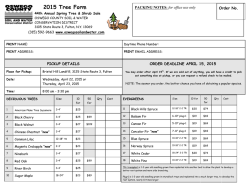
© Copyright 2026