
KASKADE7 Finite Element Toolbox Programmers Manual
K ASKADE 7 Finite Element Toolbox
Programmers Manual
M. Weiser, A. Schiela, S. G¨otschel, L. Lubkoll
B. Erdmann, L. Weimann, M. Moldenhauer, F. Lehmann
January 30, 2015
1
Contents
1
Introduction
2
Structure and Implementation
2.1 Finite Element Spaces . . .
2.2 Problem Formulation . . .
2.3 Assembly . . . . . . . . .
2.4 Adaptivity . . . . . . . . .
2.5 Time-dependent Problems
2.6 Nonlinear Solvers . . . . .
2.7 Module interaction . . . .
3
3
.
.
.
.
.
.
.
.
.
.
.
.
.
.
.
.
.
.
.
.
.
.
.
.
.
.
.
.
.
.
.
.
.
.
.
.
.
.
.
.
.
.
.
.
.
.
.
.
.
.
.
.
.
.
.
.
.
.
.
.
.
.
.
.
.
.
.
.
.
.
.
.
.
.
.
.
.
3
4
6
8
8
10
11
12
Installation and code structure
3.1 Obtaining K ASKADE 7 and third-party software
3.2 Structure of the program . . . . . . . . . . . .
3.3 Compiler und Libraries . . . . . . . . . . . . .
3.4 Using the make command . . . . . . . . . . .
3.5 Examples . . . . . . . . . . . . . . . . . . . .
3.6 Benchmarking . . . . . . . . . . . . . . . . . .
3.7 Communication with svn repository . . . . . .
.
.
.
.
.
.
.
.
.
.
.
.
.
.
.
.
.
.
.
.
.
.
.
.
.
.
.
.
.
.
.
.
.
.
.
.
.
.
.
.
.
.
.
.
.
.
.
.
.
.
.
.
.
.
.
.
.
.
.
.
.
.
.
.
.
.
.
.
.
.
13
13
14
15
16
17
18
18
.
.
.
.
.
.
.
.
.
.
.
.
.
.
.
.
.
.
.
.
.
.
.
.
.
.
.
.
.
.
.
.
.
.
.
.
.
.
.
.
.
.
.
.
.
.
.
.
.
.
.
.
.
.
.
.
.
.
.
.
.
.
.
.
.
.
.
.
.
.
4
External libraries
19
5
Documentation online
22
6
Getting started
6.1 A very first example: simplest stationary heat transfer
6.2 Example: stationary heat transfer . . . . . . . . . . .
6.2.1 A walk through the main program . . . . . .
6.2.2 Defining the functional . . . . . . . . . . . .
6.3 Example: using embedded error estimation . . . . .
6.4 Example: using hierarchical error estimation . . . . .
6.5 Example: SST pollution . . . . . . . . . . . . . . .
6.6 Example: Stokes equation . . . . . . . . . . . . . .
6.7 Example: Elasticity . . . . . . . . . . . . . . . . . .
6.8 Example: Instationary heat tranfer . . . . . . . . . .
6.9 Example: Navier-Stokes equations . . . . . . . . . .
2
.
.
.
.
.
.
.
.
.
.
.
.
.
.
.
.
.
.
.
.
.
.
.
.
.
.
.
.
.
.
.
.
.
.
.
.
.
.
.
.
.
.
.
.
.
.
.
.
.
.
.
.
.
.
.
.
.
.
.
.
.
.
.
.
.
.
.
.
.
.
.
.
.
.
.
.
.
22
23
31
33
43
47
50
54
55
56
56
60
7
Parameter administration
7.1 Introduction . . . . . . . . . . . . . . . . . . . . . . . . . . . . .
7.2 Implementation in K ASKADE 7 . . . . . . . . . . . . . . . . . .
60
60
61
8
Grid types
66
9
Linear solvers
9.1 Direct solvers . . . . . . . . . . . . . . . . . . . . . . . . . . . .
9.2 Iterative solvers, preconditioners . . . . . . . . . . . . . . . . . .
66
66
67
10 Miscellaneous
10.1 Coding Style . . . . . .
10.2 Measurement of cpu time
10.3 Namespaces . . . . . . .
10.4 Multithreading . . . . .
.
.
.
.
67
67
68
69
69
11 Details in C++ implementation
11.1 Smart pointers (std::unique ptr) . . . . . . . . . . . . . .
11.2 Fusion vectors (boost::fusion::vector) . . . . . . . . . .
69
69
69
12 The dos and don’ts – best practice
70
13 Modules
13.1 Differential operator library
13.2 Deforming grid manager .
13.2.1 Motivation . . . .
13.2.2 Getting started . .
13.2.3 Advanced usage .
.
.
.
.
.
70
71
72
72
73
75
14 Gallery of projects
14.1 Hyperthermia . . . . . . . . . . . . . . . . . . . . . . . . . . . .
75
75
15 History of K ASKADE 7 versions
15.1 K ASKADE 7.0 K ASKADE 7.1
15.2 K ASKADE 7.1 K ASKADE 7.2
75
75
75
.
.
.
.
.
.
.
.
.
.
.
.
.
.
.
.
.
.
.
.
.
.
16 K ASKADE 7 publications
.
.
.
.
.
.
.
.
.
.
.
.
.
.
.
.
.
.
.
.
.
.
.
.
.
.
.
.
.
.
.
.
.
.
.
.
.
.
.
.
.
.
.
.
.
.
.
.
.
.
.
.
.
.
.
.
.
.
.
.
.
.
.
.
.
.
.
.
.
.
.
.
.
.
.
.
.
.
.
.
.
.
.
.
.
.
.
.
.
.
.
.
.
.
.
.
.
.
.
.
.
.
.
.
.
.
.
.
.
.
.
.
.
.
.
.
.
.
.
.
.
.
.
.
.
.
.
.
.
.
.
.
.
.
.
.
.
.
.
.
.
.
.
.
.
.
.
.
.
.
.
.
.
.
.
.
.
.
.
.
.
.
. . . . . . . . . . . . . . . . . .
. . . . . . . . . . . . . . . . . .
75
3
1
Introduction
K ASKADE 7 is a general-purpose finite element toolbox for solving systems of elliptic and parabolic PDEs. Design targets for the K ASKADE 7 code have been
flexibility, efficiency, and correctness. One possibility to achieve these, to some
extent competing, goals is to use C++ with a great deal of template metaprogramming [18]. This generative programming technique uses the C++ template system
to let the compiler perform code generation. The resulting code is, due to static
polymorphism, at the same time type and const correct and, due to code generation,
adapted to the problem to be solved. Since all information relevant to code optimization is directly available to the compiler, the resulting code is highly efficient,
of course depending on the capabilities of the compiler. In contrast to explicit code
generation, as used, e.g., by the FE NI CS project [13], no external toolchain besides
the C++ compiler/linker is required. Drawbacks of the template metaprogramming
approach are longer compile times, somewhat cumbersome template notation, and
hard to digest compiler diagnostics. Therefore, code on higher abstraction levels,
where the performance gains of inlining and avoiding virtual function calls are
negligible, uses dynamic polymorphism as well.
The K ASKADE 7 code is heavily based on the D UNE libraries [2, 1, 3, 4], which
are used in particular for grid management, numerical quadrature, and linear algebra.
In Section 2 we describe the design and structure of K ASKADE 7 , also presenting some details of the implementation. The next section presents more practical
advices to use the code. In particular, we give hints how to install the code and a
set of third-party software needed in K ASKADE 7 .
Following the guideline of the sections 3, 4, and 5 the user can provide all the
technical requirements necessary to start his/her own programming. This should
be accompanied by the tutorial including a set of examples in Section 6.
Subsequent to that Getting started chapter we bring more and more details
about programming of certain classes and modules helping the user of K ASKADE 7
to extend his knowledge and get familiar to all the topics interesting for developers.
We close with a gallery of projects dealt with K ASKADE 7 , some notes on the history of development of the code, and finally a list of publications using simulation
results provided by K ASKADE 7 .
2
Structure and Implementation
As a guiding example at which to illustrate features of K ASKADE 7 we will use
in this section the all-at-once approach to the following simple optimal control
4
5
problem. For a desired state yd defined over a domain Ω ⊂ Rd , d ∈ {1, 2, 3}, and
α > 0 we consider the tracking type problem
1
y − yd
u∈L2 (Ω),y∈H01 (Ω) 2
min
2
L2 (Ω) +
α
u
2
2
L2 (Ω)
s.t.
− ∆y = u
in Ω.
The solution is characterized by the Lagrange multiplier λ ∈ H01 (Ω) satisfying the
Karush-Kuhn-Tucker system
I
∆
y
yd
α I u = 0 .
∆ I
λ
0
For illustration purposes, we will discretize the system using piecewise polynomial finite elements for y and λ and piecewise constant functions for u, even though
this is not the best way to approach this particular type of problems [11, 20].
The foundation of all finite element computation is the approximation of solutions in finite dimensional function spaces. In this section, we will discuss the
representation of functions in K ASKADE 7 before addressing the problem formulation.
2.1
Finite Element Spaces
On each reference element T0 there is a set of possibly vector-valued shape functions φi : T0 → Rs , i = 1, . . . , m defined. Finite element functions are built from
these shape functions by linear combination and transformation. More precisely,
finite element functions defined by their coefficient vectors a ∈ RN are given as
u(x)|T = ψT (x)(Φ(ξ )KT aIT ),
where aIT ∈ Rk is the subvector of a containing the coefficients of all finite element
ansatz functions which do not vanish on the element T , K ∈ Rm×k is a matrix
describing the linear combination of shape functions φi to ansatz functions ϕ j ,
Φ(ξ ) ∈ Rs×m is the matrix consisting of the shape functions’ values at the reference
coordinate ξ corresponding to the global coordinate x as columns, and ψT (x) ∈
Rs×s is a linear transformation from the values on the reference element to the
actual element T .
The indices IT and efficient application of the matrices KT and ψT (x) are provided by local-to-global-mappers, in terms of which the finite element spaces are
defined. The mappers do also provide references to the suitable shape function set,
which is, however, defined independently. For the computation of the index set IT
6
the mappers rely on the D UNE index sets provided by the grid views on which the
function spaces are defined.
For Lagrange ansatz functions, the combiner K is just a permutation matrix,
and the converter ψ(x) is just 1. For hierarchical ansatz functions in 2D and
3D, nontrivial linear combinations of shape functions are necessary. The implemented over-complete hierarchical FE spaces require just signed permutation matrices [21]. Vectorial ansatz functions, e.g. edge elements, require nontrivial converters ψ(x) depending on the transformation from reference element to actual element. The structure in principle allows to use heterogeneous meshes with different
element topology, but the currently implemented mappers require homogeneous
meshes of either simplicial or quadrilateral type.
In K ASKADE 7 , finite element spaces are template classes parameterized with
a mapper, defining the type of corresponding finite element functions and supporting their evaluation as well as prolongation during grid refinement, see Sec. 2.4.
Assuming that View is a suitable D UNE grid view type, FE spaces for the guiding
example can be defined as:
typedef
typedef
H1Space
L2Space
FEFunctionSpace<ContinuousLagrangeMapper<double,View> > H1Space;
FEFunctionSpace<DiscontinuousLagrangeMapper<double,View> > L2Space;
h1Space(gridManager,view,order);
l2Space(gridManager,view,0);
Multi-component FE functions are supported, which gives the possibility to
have vector-valued variables defined in terms of scalar shape functions. E.g., displacements in elastomechanics and temperatures in the heat equation share the
same FE space. FE functions as elements of a FE space can be constructed using
the type provided by that space:
H1Space::Element<1>::type y(h1Space), lambda(h1Space);
L2Space::Element<1>::type u(l2Space);
FE functions provide a limited set of linear algebra operations. Having different types for different numbers of components detects the mixing of incompatible
operands at compile time.
During assembly, the ansatz functions have to be evaluated repeatedly. In
order not to do this separately for each involved FE function, FE spaces define
Evaluators doing this once for each involved space. When several FE functions
need to be evaluated at a certain point, the evaluator caches the ansatz functions’
values and gradients, such that the remaining work is just a small scalar product
for each FE function.
7
2.2
Problem Formulation
For stationary variational problems, the K ASKADE 7 core addresses variational
functionals of the type
min
ui ∈Vi Ω
F(x, u1 , . . . , un , ∇u1 , . . . , ∇un ) dx +
G(x, u1 , . . . , un ) ds.
(1)
∂Ω
In general, this problem is nonlinear. Therefore we formulate the Newton iteration in order to find the solution u = (u1 , . . . , un )T :
Starting with an initial guess u0 for u we compute the Newton update δ u by
F (u0 )[δ u, v] dx+
Ω
G (u0 )[δ u, v] ds =
∂Ω
F (u0 )v dx+
Ω
G (u0 )v ds
∂Ω
∀v ∈ V
(2)
The approximation after one step is
unew = u0 − δ u.
The problem definition consists of providing F, G, and their first and second directional derivatives in a certain fashion. First, the number of variables, their number
of components, and the FE space they belong to have to be specified. This partially static information is stored in heterogeneous, statically polymorphic containers from the B OOST F USION [5] library. Variable descriptions are parameterized
over their space index in the associated container of FE spaces, their number of
components, and their unique, contiguous id in arbitrary order.
typedef boost::fusion::vector<H1Space*,L2Space*> Spaces;
Spaces spaces(&h1Space,&l2Space);
typedef boost::fusion::vector<
Variable<SpaceIndex<0>,Components<1>,VariableId<0> >,
Variable<SpaceIndex<0>,Components<1>,VariableId<1> >,
Variable<SpaceIndex<1>,Components<1>,VariableId<2> > > VarDesc;
Besides this data, a problem class defines, apart from some static meta information, two mandatory member classes, the DomainCache defining F and the
BoundaryCache defining G. The domain cache provides member functions d0,
d1, and d2 evaluating F(·), F (·)vi , and F (·)[vi , w j ], respectively. For the guiding
example with
1
α
F = (y − yd )2 + u2 + ∇λ T ∇y − λ u,
2
2
the corresponding code looks like
8
double d0() const {
return (y-yd)*(y-yd)/2 + u*u*alpha/2 + dlambda*dy lambda*u;
}
template <int i, int d>
double d1(VariationalArg<double,d> const& vi) const {
if (i==0) return (y-yd)*vi.value + dlambda*vi.gradient;
if (i==1) return alpha*u*vi.value - lambda*vi.value;
if (i==2) return dy*vi.gradient - u*vi.value;
}
template <int i, int j, int d>
double d2(VariationalArg<double,d> const& vi,
VariationalArg<double,d> const& wj) const {
if (i==0 && j==0) return vi.value*wj.value;
if (i==0 && j==2) return vi.gradient*wj.gradient;
if (i==1 && j==1) return alpha*vi.value*wj.value;
if (i==1 && j==2) return -vi.value*wj.value;
if (i==2 && j==0) return vi.gradient*wj.gradient;
if (i==2 && j==1) return -vi.value*wj.value;
}
A static member template class D2 defines which Hessian blocks are available.
Symmetry is auto-detected, such that in d2 only j ≤ i needs to be defined.
template <int row, int col>
class D2 {
static int present = (row==2) || (row==col);
};
The boundary cache is defined analogously.
The functions for y, u, and λ are specified (for nonlinear or instationary problems in form of FE functions) on construction of the caches, and can be evaluated
for each quadrature point using the appropriate one among the evaluators provided
by the assembler:
template <class Pos, class Evaluators>
void evaluateAt(Pos const& x, Evaluators const&
evaluators) {
y = yFunc.value(at_c<0>(evaluators));
u = uFunc.value(at_c<1>(evaluators));
lambda = lambdaFunc.value(at_c<0>(evaluators));
dy = yFunc.gradient(at_c<0>(evaluators));
dlambda = lambdaFunc.gradient(at_c<0>(evaluators));
}
9
Hint. Usage of at_c<int>
The function at_c<int>() allows one to access the elements of a heterogeneous array, that is an array, with possibly different data types (as opposed to the
std::array, where the data type is fixed at initialisation to one type). An example for this is above in the method evaluateAt(). The data type evaluators
contains evaluators of different type for the continuous H1 space used for state y
and the discontinuous L2 space used for the control u. Having different types,
the evaluators cannot be stored in a homogeneous array such as std::vector
or std::array. Hence the at c method allows to access both evaluators. The
call at_c<0>(evaluators) reaches the first element of evaluators, while
at_c<1>(evaluators) accesses the second and so forth.
2.3
Assembly
Assembly of matrices and right-hand sides for variational functionals is provided
by the template class VariationalFunctionalAssembler, parameterized
with a (linearized) variational functional. The elements of the grid are traversed.
For each cell, the functional is evaluated at the integration points provided by a
suitable quadrature rule, assembling local matrices and right-hand sides. If applicable, boundary conditions are integrated. Finally, local data is scattered into global
data structures. Matrices are stored as sparse block matrices with compressed row
storage, as provided by the D UNE BCRSMatrix<BlockType> class. For evaluation of FE functions and management of degrees of freedom, the involved spaces
have to be provided to the assembler. User code for assembling a given functional
will look like the following:
boost::fusion::vector<H1Space*,L2Space*> spaces(&h1space, &l2space);
VariationalFunctionalAssembler<Functional> as(spaces);
as.assemble(linearization(f,x));
For the solution of the resulting linear systems, several direct and iterative
solvers can be used through an interface to D UNE -I STL. For instance, the D UNE
AssembledLinearOperator interface is provided by the K ASKADE 7 class
AssembledGalerkinOperator. After the assembly, and some more initializations (rhs, solution), e.g. a direct solver directType can be applied:
AssembledGalerkinOperator A(as);
directInverseOperator(A,directType).applyscaleadd(-1.,rhs,solution);
2.4
Adaptivity
K ASKADE 7 provides several means of error estimation.
10
Embedded error estimator. Given a FE function u, an approximation of the
error can be obtained by projecting u onto the ansatz space with polynomials of
order one less. The method embeddedErrorEstimator() then constructs
(scaled) error indicators, marks cells for refinement and adapts the grid with aid of
the GridManager class, which will be described later.
error = u;
projectHierarchically(variableSet, u);
error -= u;
accurate = embeddedErrorEstimator(variableSet,error,u,scaling,tol,gridManager);
Hierarchic error estimator. After discretization using a FE space Sl , the minimizer of the variational functional satisfies a system of linear equations, All xl =
−bl . For error estimation, the ansatz space is extended by a second, higher order
ansatz space, Sl ⊕Vq . The solution in this enriched space satisfies
All Alq
Aql Aqq
xl
b
=− l .
xq
bq
Of course the solution of this system is quite expensive. As xl is essentially
known, just the reduced system diag(Aqq )xq = −(bq +Aql xl ) is solved [8]. A global
error estimate can be obtained by evaluating the scalar product xq , bq .
In K ASKADE 7 , the template class HierarchicErrorEstimator is available. It is parameterized by the type of the variational functional, and the description of the hierarchic extension space. The latter can be defined using e.g. the
ContinuousHierarchicExtensionMapper. The error estimator then can
be assembled and solved, analogously to the assembly and solution of the original
variational functional.
Grid transfer. Grid transfer makes heavy use of the signal-slot concept, as implemented in the B OOST.S IGNALS library [5]. Signals can be seen as callback
functions with multiple targets. They are connected to so-called slots, which are
functions to be executed when the signal is sent. This paradigm allows to handle
grid modifications automatically, ensuring that all grid functions stay consistent.
All mesh modifications are done via the GridManager<Grid> class, which
takes ownership of a grid once it is constructed. Before adaptation, the grid manager triggers the affected FE spaces to collect necessary data in a class TransferData. For all cells, a local restriction matrix is stored, mapping global degrees
of freedom to local shape function coefficients of the respective father cell. After grid refinement or coarsening, the grid manager takes care that all FE functions are transfered to the new mesh. Since the construction of transfer matrices
11
from grid modifications is a computationally complex task, these matrices are constructed only once for each FE space. On that account, FE spaces listen for the
GridManager’s signals. As soon as the transfer matrices are constructed, the FE
spaces emit signals to which the associated FE functions react by updating their
coefficient vectors using the provided transfer matrix. Since this is just an efficient
linear algebra operation, transfering quite a lot of FE functions from the same FE
space is cheap.
After error estimation and marking, the whole transfer process is initiated in
the user code by:
gridManager.adaptAtOnce();
The automatic prolongation of FE functions during grid refinement makes it particularly easy to keep coarser level solutions at hand for evaluation, comparison,
and convergence studies.
2.5
Time-dependent Problems
K ASKADE 7 provides an extrapolated linearly implicit Euler method for integration of time-dependent problems B(y)y˙ = f (y), [9]. Given an evolution equation
Equation eq, the corresponding loop looks like
Limex<Equation> limex(gridManager,eq,variableSet);
for (int steps=0; !done && steps<maxSteps; ++steps) {
do {
dx = limex.step(x,dt,extrapolOrder,tolX);
errors = limex.estimateError(/*...*/);
// ... (choose optimal time step size)
} while( error > tolT );
x += dx ;
}
Step computation makes use of the class SemiImplicitEulerStep. Here,
the stationary elliptic problem resulting from the linearly implicit Euler method
is defined. This requires an additional method b2 in the domain cache for the
evaluation of B. For the simple scalar model problem with B(x) independent of y,
this is just the following:
template<int i, int j, int d>
Dune::FieldMatrix<double, TestVars::Components<i>::m, AnsatzVars::Components<j>::m>
b2(VariationalArg<double,d> const& vi, VariationalArg<double,d> const& wj) const {
return bvalue*vi.value*vj.value;
}
Of course, bvalue has to be specified in the evaluateAt method.
12
2.6
Nonlinear Solvers
A further aspect of K ASKADE 7 is the solution of nonlinear problems, involving
partial differential equations. Usually, these problems are posed in function spaces,
which reflect the underlying analytic structure, and thus algorithms for their solution should be designed to inherit as much as possible from this structure.
Algorithms for the solution of nonlinear problems of the form (1) build upon
the components described above, such as discretization, iterative linear solvers, and
adaptive grid refinement. A typical example is Newton’s method for the solution
of a nonlinear operator equation. Algorithmic issues are the adaptive choice of
damping factors, and the control of the accuracy of the linear solvers. This includes
requirements for iterative solvers, but also requirements on the accuracy of the
discretization.
The interface between nonlinear solvers and supporting routines is rather coarse
grained, so that dynamic polymorphism is the method of choice. This makes it possible to develop and compile complex algorithms independently of the supporting
routines, and to reuse the code for a variety of different problems. In client code
the components can then be plugged together, and decisions are made, which type
of discretization, linear solver, adaptivity, etc. is used together with the nonlinear
algorithm. In this respect, K ASKADE 7 provides a couple of standard components,
but of course users can write their own specialized components.
Core of the interface are abstract classes for a mathematical vector, which supports vector space operations, but no coordinatewise access, abstract classes for
norms and scalar products, and abstract classes for a nonlinear functional and its
linearization (or, more accurately, its local quadratic model). Further, an interface
for inexact linear solvers is provided. These concepts form a framework for the
construction of iterative algorithms in function space, which use discretization for
the computation of inexact steps and adaptivity for error control.
In order to apply an algorithm to the solution of a nonlinear problem, one can
in principle derive from these abstract classes and implement their purely virtual
methods. However, for the interaction with the other components of K ASKADE 7 ,
bridge classes are provided, which are derived from the abstract base classes, and
own an implementation.
We explain this at the following example which shows a simple implementation
of the damped Newton method:
for(int step=1; step <= maxSteps; step++) {
lin = functional->getLinearization(*iterate);
linearSolver->solve(*correction,*lin);
do {
*trialIter = *iterate;
13
trialIter->axpy(dampingFactor,*correction);
if(regularityTest(dampingFactor)==Failed) return -1;
updateDampingFactor(dampingFactor);
}
while(evalTrialIterate(*trialIter,*correction,*lin)==
Failed);
*iterate = *trialIter;
if(convergenceTest(*correction,*iterate)==Achieved)
return 1;
}
While regularityTest, updateDampingFactor, evalTrialIterate,
and convergenceTest are implemented within the algorithm, functional,
lin, and linearSolver, used within the subroutines are instantiations of derived classes, provided by client code. By
linearSolver->solve(*correction,*lin);
a linear solver is called, which has access to the linearization lin as a linear operator equation. It may either be a direct or an iterative solver on a fixed discretization, or solve this operator equation adaptively, until a prescribed relative accuracy
is reached. In the latter case, the adaptive solver calls in turn a linear solver on each
refinement step. There is a broad variety of linear solvers available, and moreover,
it is not difficult to implement a specialized linear solver for the problem at hand.
The object lin is of type AbstractLinearization, which is implemented by the bridge class Bridge::KaskadeLinearization. This bridge
class is a template, parametrized by a variational functional and a vector of type
VariableSet::Representation. It uses the assembler class to generate
the data needed for step computation and manages generated data. From the client
side, only the variational functional has to be defined and an appropriate set of
variables has to be given.
Several algorithms are currently implemented. Among them there is a damped
Newton method [7] with affine covariant damping strategy, a Newton path-following
algorithm, and algorithms for nonlinear optimization, based on a cubic error model.
This offers the possibility to solve a large variety of nonlinear problems involving
partial differential equations. As an example, optimization problems with partial
differential equations subject to state constraints can be solved by an interior point
method combining Newton path-following and adaptive grid refinement [16].
2.7
Module interaction
Figure 1 shows the interaction between the described modules.
14
!
" ! #
!
IO
$!
(
!
$
!
$ !
%
$
'
$ !
&&&
dynamic (
) and static (
) polymorphism
Figure 1: Module interaction
3
Installation and code structure
3.1
Obtaining K ASKADE 7 and third-party software
K ASKADE 7 is maintained by the Apache revision control system SVN and is
hosted on the server https://svn.zib.de/. To obtain a working copy of K ASKADE 7
from the ZIB SVN repository, change to the directory wherein you want to create
the working copy subdirectory and enter the command
svn co https://[email protected]/zibDUNE/Kaskade7.2
or
svn co --username user https://svn.zib.de/zibDUNE/Kaskade7.2
where you substitute user by your ZIB SVN userid. If you intend to run your
K ASKADE 7 copy on a 64-bit Linux system at the ZIB (e.g., on a machine of
the HTC cluster), just change into the K ASKADE 7 directory, create a suitable
file named Makefile.Local, by creating a copy of Makefile-htc.Local
with this name and changing the macros KASKADE7 and for a non-htc machine
also INSTALLS. Set the environment variables PATH and LD LIBRARY PATH
to suitable values (see below) and type
15
make install
If you intend to run K ASKADE 7 on some other system, you need to install on
this system a suitable compiler and other thirdparty software which is needed by
K ASKADE 7 . To fulfil this task, get from the ZIB repository the K ASKADE 7 software installer by the following command
svn co https://[email protected]/zibDUNE/Install_Kaskade7
Then change to the Install Kaskade7 directory and use some install-xxx.Local
file as a template for the install.Local file which you need to create. Review
the install.Local file and perhaps adapt it to your installation needs (for example the name and location of your LAPACK/BLAS library). For a LINUX 64bit
system, we recommend to use the ACML library from http://developer.amd.com/toolsand-sdks/cpu-development/amd-core-math-library-acml/acml-downloads-resources/
as LAPACK/BLAS replacement.
Please, also read the file README BEFORE STARTING, and check for availability of the prerequites mentioned in this file. Also, take special attention to other
notes marked by ∗ ∗ ∗ . Doing so may perhaps save you a lot of time in case of
unexpected errors during the installation run. Finally, run the command
./install.sh
The ./install.sh shellscript will prompt you for some needed information,
and then install all required third-party software. As the last step, the shellscript
will also create a suitable Makefile.Local in the K ASKADE 7 directory, and run the
commands
make install
If you have installed Alberta during the previous installation run, then before
you can use Kaskade7.2 with AlbertaGrid, you will need to make some small modifications to header-files of Kaskade7.2 and some thirdpartysoftware. For details,
read the file ALBERTA IMPORTANT HINTS.txt in the installer-directory.
3.2
Structure of the program
After checking out the program to directory KASKADE7 we have the following
structure of the source code stored into corresponding subdirectories.
• KASKADE7/algorithm
• KASKADE7/fem
16
• KASKADE7/io
• KASKADE7/ipopt
• KASKADE7/linalg
• KASKADE7/timestepping
• KASKADE7/mg
• KASKADE7/tutorial
• KASKADE7/problems
• KASKADE7/experiments
• KASKADE7/benchmarking
• KASKADE7/tests
In these subdirectories we find .hh- and .cpp- files, some auxiliary files and
sometimes further subdirectories. In directories including .cpp- files there is a
Makefile generating object files or libraries which are stored into KASKADE7/libs.
3.3
Compiler und Libraries
Before calling make in KASKADE7 directory or in one of the subdirectories the
user should make sure that the correct compiler (corresponding to the selection
in the Makefiles) is available. In the installation at ZIB this can be provided by
modifying the PATH variable, e.g.,
setenv PATH /home/datanumerik/archiv/software/linux64/gcc-$VERSION_GCC/gcc/bin:$PATH
where we have to set V ERSION GCC to ”4.9.0” in version 7.2 of K ASKADE 7
(note that the given paths (/home/datanumerik/. . . ) are adjusted to htc use).
In order to assure that all needed Shared Libraries are found we have to set the
LD LIBRARY PATH variable:
setenv LD_LIBRARY_PATH "/home/datanumerik/archiv/software/linux64/gfortran64/lib:
/home/datanumerik/archiv/software/linux64/gcc-$VERSION_GCC/gcc/lib64:
/home/datanumerik/archiv/software/linux64/gcc-$VERSION_GCC/gcc/lib:
/home/datanumerik/archiv/software/linux64/gcc-$VERSION_GCC/alberta-3.0.0/lib:
/home/datanumerik/archiv/software/linux64/gcc-$VERSION_GCC/boost-$VERSION_BOOST/lib"
or similar in a bash shell:
17
LD_LIBRARY_PATH="/home/datanumerik/archiv/software/linux64/gfortran64/lib:
/home/datanumerik/archiv/software/linux64/gcc-$VERSION_GCC/gcc/lib64:
/home/datanumerik/archiv/software/linux64/gcc-$VERSION_GCC/gcc/lib:
/home/datanumerik/archiv/software/linux64/gcc-$VERSION_GCC/alberta-3.0.0/lib:
/home/datanumerik/archiv/software/linux64/gcc-$VERSION_GCC/boost-$VERSION_BOOST/lib"
export LD_LIBRARY_PATH
V ERSION BOOST is set to ”1.51.0” in K ASKADE 7 version 7.2.
The library path is used by the ACML Library (BLAS und LAPACK), the compile
library, libmpfr.so.1 (used when the compiler is called), the BOOST 1.51.0 libraries
and the ALBERTA 3.0.0 Library.
Note: on MacOS X machines we have to set the variable DYLD LIBRARY PATH
with the corresponding paths.
3.4
Using the make command
Makefile.Local. In the root directory KASKADE7 the user has to write a file
Makefile.Local including paths to third-party software, compilers, as well
as flags for compiler and debugger. In particular, the full path of the KASKADE7
directory has to be defined. There are example files like Makefile-htc.Local
and Makefile-mac.Local which can be copied for use on HTC- resp. Macmachines.
make in the KASKADE directory. In the root directory KASKADE the Makefile may be called with different parameters:
• make clean removes all object files, executables, and some other files.
• make depend generates the Makefile in tarball distribution subdirectories
which includes dependencies to c++ headerfiles of KASKADE and (maybe)
some third-party software.
• make experimentsdepend generates the Makefile in some subdirectories
of the experiments directory which includes dependencies to c++ headerfiles
of KASKADE and (maybe) some third-party software.
• make kasklib generates object files and builds the library libkaskade.a.
• make install combines the two commands make depend and make kasklib.
• make experiments builds and executes the examples in the experiments
directory.
• make tutorial builds and executes the examples in the tutorial , and
builds the pdf version of the manual.
18
• make cleantutorial removes all object files, executables, and some other
files in the subdirectories.
• make benchmarks builds and executes the examples in the benchmarking
subdirectories.
• make distribution generates tar.gz - files after executing make clean, ignoring SVN information, documentation, and particular subdirectories.
For installing the complete K ASKADE 7 use the four top make commands from
above in the order specified: clean, depend, kasklib, tutorial. Note, that first
some shell variables (i.e., PAT H and LD LIBRARY PAT H) have to be defined as
described in the paragraph 3.3.
make in subdirectory. Once you have a complete installation of K ASKADE 7 it
may be necessary (after changing a file) to recompile in a subdirectory and update
the K ASKADE 7 library. This is done by using the file Makefile in the corresponding subdirectory. You just have to type make.
Note, that after checking out the code from the repository there are no files
Makefile in the subdirectories but only files called Makefile.gen. Such a
Makefile.gen can be used to generate a corresponding Makefile by typing:
• make -f Makefile.gen depend
Thus the dependencies are detected and registered in the Makefile. Each Makefile.gen
includes a depend and a clean option. Note that a call make depend in the
KASKADE directory also generates the local Makefile from the local Makefile.gen
in each of the subdirectories mentioned in the Makefile.
3.5
Examples
Applications of the K ASKADE 7 software can be found in the subdirectories
• KASKADE7/tutorial
• KASKADE7/experiments
• KASKADE7/problems
Each of these subdirectories needs a Makefile.gen with the properties mentioned above. In the subdirectory KASKADE7/tutorial you find examples
which are described in detail in this manual starting with Section 6.
19
The subdirectory KASKADE7/experiments includes more or less the same examples as the tutorial subdirectory. These examples uld be used to test any changes
in the base code of K ASKADE 7 . No modification in the tutorial code should be
committed to the svn repository The subdirectory KASKADE7/experiments/moreExamples
may be used for examples still under construction.
More examples can be found in subdirectory KASKADE7/problems, but without
annotation. In particular, you find here the current projects of developers.
3.6
Benchmarking
The directory KASKADE7/benchmarking provides a set of test examples. In
addition to the examples in the tutorial we investigate here not only if the computation is running but also if it computes the correct results.
The benchmarking is started in the K ASKADE 7 root directory by typing
• make benchmarks
The results will be summarized in the file testResult.txt.
3.7
Communication with svn repository
Above in this section we described how to get a copy from the K ASKADE 7 repository by the shell command
svn co https://[email protected]/zibDUNE/Kaskade7.2
This copy can be used for arbitrary applications. Any change by the user is allowed.
But it is always under certain control of the svn system, i.e. the version control system svn registers all differences between repository and local copy. Furthermore,
svn provides a set of commands to communicate between the local copy of a user
and the current state of the repository. Thus there are svn commands to add a new
file into the repository, to delete a file from the repository, to update local files or
to commit local changes to the repository.
Enter the command
svn help
in your shell to get a first idea of the options offered by svn:
%svn help
usage: svn <subcommand> [options] [args]
Subversion command-line client, version 1.6.17.
Type ’svn help <subcommand>’ for help on a specific subcommand.
Type ’svn --version’ to see the program version and RA modules
20
or ’svn --version --quiet’ to see just the version number.
Most subcommands take file and/or directory arguments, recursing
on the directories. If no arguments are supplied to such a
command, it recurses on the current directory (inclusive) by default.
Available subcommands:
add
blame (praise, annotate, ann)
cat
changelist (cl)
checkout (co)
cleanup
commit (ci)
copy (cp)
delete (del, remove, rm)
diff (di)
export
help (?, h)
import
info
list (ls)
lock
log
merge
mergeinfo
mkdir
move (mv, rename, ren)
propdel (pdel, pd)
propedit (pedit, pe)
propget (pget, pg)
proplist (plist, pl)
propset (pset, ps)
resolve
resolved
revert
status (stat, st)
switch (sw)
unlock
update (up)
Subversion is a tool for version control.
For additional information, see http://subversion.tigris.org/
%
The correct syntax of all these svn commands can easily be found in the internet,
e.g., http://subversion.tigris.org/.
4
External libraries
• ALBERTA: Directory alberta-3.0.1/lib (optional)
21
– libalberta 3d.a
ALBERTA 3D-grid routines.
– libalberta 2d.a
ALBERTA 2D-grid routines.
– libalberta 1d.a
ALBERTA 1D-grid routines.
– libalberta utilities.a
ALBERTA common utilities routines.
• ALUGRID: Directory ALUGrid-1.52/lib (optional)
– libalugrid.a
ALUGRID FEM grid-library.
• AMIRAMESH: Directory libamira/lib
– libamiramesh.a
Reading and writing Amiramesh files.
• BOOST: Directory boost-1.57.0/lib
– libboost signals.SUFFIX
Managed signals and slots callback implementation.
– libboost program options.SUFFIX
The program options library allows program developers to obtain program options, that is (name, value) pairs from the user, via conventional
methods such as command line and config file.
– libboost program system.SUFFIX
Operating system support, including the diagnostics support that will
be part of the C++0x standard library.
– libboost program timer.SUFFIX
Event timer, progress timer, and progress display classes.
– libboost program thread.SUFFIX
Portable C++ multi-threading.
– libboost program chrono.SUFFIX
Useful time utilities.
– SUFFIX is so under Linux and dylib under MacOS X (Darwin)
• DUNE: Directory dune-2.3.1/lib
22
– libdunecommon.a
DUNE common modules.
– libdunegeometry.a
DUNE geometry modules.
– libdunegrid.a
DUNE grid methods.
– libdunealbertagrid 3d.a
DUNE interface to ALBERTA 3D-grid routines. (optional)
– libdunealbertagrid 2d.a
DUNE interface to ALBERTA 2D-grid routines. (optional)
– libdunealbertagrid 1d.a
DUNE interface to ALBERTA 1D-grid routines. (optional)
– libdunegridglue.a
DUNE library for contact-problems (optional)
• HYPRE: Directory hypre-2.8.0b/lib
– libHYPRE.a
• ITSOL: Directory itsol-1/lib
– libitsol.a
• MUMPS: Directory mumps-4.10.0/lib
Direct sparse linear solver library.
– libdmumps.a
– libmpiseq.a
– libmumps common.a
– libpord.a
– libpthread.a
• SUPERLU: Directory superlu-4.3/lib
Direct sparse linear solver library.
– libsuperlu.a
• TAUCS: Directory taucs-2.0/lib
Preconditioner library.
– libtaucs.a
23
• UG for DUNE: Directory dune-2.3.1/lib
UG for DUNE, FEM grid-library.
– libugS3.a
– libugS2.a
– libugL3.a
– libugL2.a
– libdevS.a
– libdevX.a
• UMFPACK: Directory umfpack-5.4.0/lib
Direct sparse linear solver library.
– libumfpack.a
– libamd.a
5
Documentation online
In subdirectory Kaskade7/doc there is a script makeDocu for generating a documentation of the source code. Necessary is the program doxygen and a Latex
installation. Outline and shape of the documentation is steered by the doxygen
parameter file called Doxyfile.
By default ( GENERAT E HT ML = Y ES ) the generation of HTML pages is
selected. The source files to be analysed are defined via INPUT variable.
If the auxiliary program dot of the GraphViz software is available, we recommend to change the preset HAV E DOT = NO to HAV E DOT = Y ES in the file
Doxyfile.
After generating the documentation ( by command makeDocu ) the pages may
be considered in the browser by specifying the full path .../kaskade7/doc/html/index.html.
6
Getting started
In this chapter we present a set of examples which enable a user wihout any experiences in K ASKADE 7 to get started. In particular, the first example should specify
all the steps to understand the technical handling of K ASKADE 7 independent of
know-how about numerics and implementation. The following examples give more
and more details bringing together the mathematical formulation of a problem and
its implementation.
24
6.1
A very first example: simplest stationary heat transfer
This example is implemented in subdirectory
KASKADE7/tutorial/laplacian
Files: laplace.cpp, laplace.hh, Makefile
We compute the solution u of the Laplacian or Poisson equation
−∇ · (∇u) = 1
u=0
x ∈Ω
on Γ
(3)
on the two-dimensional open unit square Ω under homogeneous boundary conditions on Γ = ∂ Ω. These equations may describe stationary heat transfer caused by
a constant heat source (value 1 on the right-hand side) and constant temperature
(0oC) on the boundary, e.g. by cooling.
Resolving the ∇ - operator in the equation (3), we also can write in cartesian
coordinates x and y
−
∂ 2u ∂ 2u
−
=1
∂ x 2 ∂ y2
u=0
(x,y) ∈ (0, 1) 1)
(4)
on Γ
The treatment of this problem in context of finite element methods as used in
K ASKADE 7 is based on a variational formulation of the equation (3) and needs to
¯ (including the boundary), a set of ansatz
provide a triangulation of the domain Ω
functions (order 1: linear elements, order 2: quadratic elements,...), functions for
evaluating the integrands in the weak formulation, assembling of the stiffness matrix and right-hand side. All this is to be specified in the files laplace.cpp and
laplace.hh using the functionality of the K ASKADE 7 library. Shortly, we will explain details and possibilities to change the code.
Once accepted the code, the user has to compile and to generate the executable
by calling the Makefile (recall that the Makefile was generated already by the installation procedure as introduced in Section 3). which is already in the same directory.
Just enter the command
make laplace
or simply
make
If this make procedure works without errors you get the executable file laplace
which can be performed by the command
25
./laplace
The program sends some messages to the terminal (about progress of the calculation) and writes graphical information (mesh and solution data) to a file temperature.vtu. This file can be visualized by any tool (e.g., paraview) which can
interprete vtk format.
The shell command
make clean
deletes the files laplace, laplace.o, temperature.vtu, and gccerr.txt. The last one
is only generated if an error or warnings are discovered by the compiler. Then it
includes all the error messages and warnings which offers a more comfortable way
to analyse the errors than to get all to the terminal.
We summarize: In order to get a running code which computes a finite element
soluton of the Lapacian problem (3) only the three commands
make clean
make
./laplace
have to be entered.
Now we explain the fundamentals of treating problems like (3) in K ASKADE 7.
Using the notation from Section 2.2 we have in this example
1
F(u) = ∇uT ∇u − f u
2
and
1
G(u) = (u − u0 )2 , u0 = 0
2
and solving of Equation (3) results in:
Compute a solution of the minimization problem (1) by a Newton iteration solving
in each step the following problem:
Find u ∈ V ⊂ H01 (Ω) with
d2Ω (u, v) dx +
Ω
d2Γ (u, v) ds =
Γ
d1Ω (v) dx +
Ω
d1Γ (v) ds
∀v ∈ V,
Γ
d1Ω (v), d2Ω (v) evaluating F (·)(v) and F (·)(v, w) respectively, i.e., the first and
second derivative of the integrand d0Ω (v) = F(v) as already shown in Section
2.2. Analogously, we determine d1Γ (v), d2Γ (v) as G (·)(v) and G (·)(v, w) respectively.
26
In our context V is always a finite element space spanned by the base functions {ϕi }1s,N , N is the dimension of the space. That means, we have to solve the
following system of N equations in order to find the minim in the space V :
d2Ω (u, ϕi ) dx+
Ω
d2Γ (u, ϕi ) ds =
Γ
d1Ω (ϕi )+
Ω
d1Γ (ϕi ) ds
Γ
for ϕi , i = 1s, N.
(5)
Here we have
1 T
∇u ∇u − f u
2
d1Ω (ϕi ) = ∇uT ∇ϕi − f ϕi
d0Ω () =
Ω
d2 (ϕi , ϕ j ) =
∇ϕiT ∇ϕ j
(6)
(7)
(8)
in the region Ω, and
1
(u − u0 )2
2
d1Γ (ϕi ) = γ (u − u0 )ϕi
d0Γ () = γ
Γ
d2 (ϕi , ϕ j ) = γ ϕi ϕ j
(9)
(10)
(11)
on the boundary Γ. The term γ is a penalty term ensuring numerical accuracy and
should be large (e.g. 109 ).
These functions have to be defined in two mandatory classes in the problem
class (called HeatFunctional): the DomainCache defining d0Ω (), d1Ω (), and d2Ω ()
for the region Ω, and the BoundaryCache defining d0Γ () = G and its derivatives
on the boundary Γ = ∂ Ω.
In general the functional to be minimized is nonlinearly depending on the solution u. However, in this example it is linear, so that already the first step in the
Newton method provides the solution, implemented in the main() as shown below.
In case of a nonlinear functional we have to write a complete Newton loop controlling the size of the update and stopping if it is small enough. We present such an
example (from elasticity) later in this chapter.
Now, we focus on the specific details of implementation for our Laplacian
problem which can be found in the files laplace.cpp and laplace.hh. We are not
trying to explain everything. Just some hints to the essentials in order to get a first
feeling for the code.
The code in the main program (file laplace.cpp)
int main(int argc, char *argv[])
27
{
...
std::cout << "Start Laplacian tutorial program" << std::endl;
int const dim=2;
// spatial dimension of domain
std::cout << "dimension of space:
" << dim << std::endl;
int refinements = 5,
// refinements of initial mesh
order = 2;
// dimension of finite element space
std::cout << "original mesh shall be refined: " << refinements << " times" << std::endl;
std::cout << "discretization order
: " << order << std::endl;
...
}
sets some parameters and comprises the following essential parts:
• definition of a triangulation of the region Ω
//
two-dimensional space: dim=2
typedef Dune::UGGrid<dim> Grid;
Dune::GridFactory<Grid> factory;
// vertex coordinates v[0], v[1]
Dune::FieldVector<double,dim> v;
v[0]=0;
v[1]=0;
factory.insertVertex(v);
v[0]=1;
v[1]=0;
factory.insertVertex(v);
v[0]=1;
v[1]=1;
factory.insertVertex(v);
v[0]=0;
v[1]=1;
factory.insertVertex(v);
v[0]=0.5; v[1]=0.5; factory.insertVertex(v);
// triangle defined by 3 vertex indices
std::vector<unsigned int> vid(3);
Dune::GeometryType gt(Dune::GeometryType::simplex,2);
vid[0]=0; vid[1]=1; vid[2]=4; factory.insertElement(gt,vid);
vid[0]=1; vid[1]=2; vid[2]=4; factory.insertElement(gt,vid);
vid[0]=2; vid[1]=3; vid[2]=4; factory.insertElement(gt,vid);
vid[0]=3; vid[1]=0; vid[2]=4; factory.insertElement(gt,vid);
// a gridmanager is constructed
// as connector between geometric and algebraic information
GridManager<Grid> gridManager( factory.createGrid() );
gridManager.enforceConcurrentReads(true);
// the coarse grid will be refined times
gridManager.globalRefine(refinements);
The parameter refinements defined in top of the main program determines
how often the coarse grid defined here has to be refined uniformly. The
resulting mesh is the initial one for the following computation. In context
of adaptive mesh refinement it might be object of further refinements, see
example in subsection 6.3.
• definition of the finite element space
28
// construction of finite element space for the scalar solution u.
typedef FEFunctionSpace<ContinuousLagrangeMapper<double,LeafView> > H1Space;
H1Space temperatureSpace(gridManager,gridManager.grid().leafView(),order);
typedef boost::fusion::vector<H1Space const*> Spaces;
Spaces spaces(&temperatureSpace);
//
//
//
//
//
construct variable list.
VariableDescription<int spaceId, int components, int Id>
spaceId: number of associated FEFunctionSpace
components: number of components in this variable
Id: number of this variable
typedef boost::fusion::vector<Variable<SpaceIndex<0>,Components<1>,VariableId<0> > >
VariableDescriptions;
std::string varNames[1] = { "u" };
typedef VariableSetDescription<Spaces,VariableDescriptions> VariableSet;
VariableSet variableSet(spaces,varNames);
Here we define the finite element space underlying the discretization of our
equation (5) corresponding to the introduction in Section 2.1. The parameter
order defined in top of the main program specifies the order of the finite
element space in the statement
H1Space temperatureSpace(gridManager,gridManager.grid().leafView(),order);
• definition of the variational functional
// construct variational functional
typedef HeatFunctional<double,VariableSet> Functional;
Functional F;
// some interesting parameters:
// number of variables, here 1
// number of equations, here 1
// number of degrees of freedom, depends on order
int const nvars = Functional::AnsatzVars::noOfVariables;
int const neq = Functional::TestVars::noOfVariables;
std::cout << "no of variables = " << nvars << std::endl;
std::cout << "no of equations = " << neq
<< std::endl;
size_t dofs = variableSet.degreesOfFreedom(0,nvars);
std::cout << "number of degrees of freedom = " << dofs << std::endl;
The code defining the functional can be found in the file laplace.hh. The
corresponding class is called HeatFunctional and contains the mandatory
members DomainCache and BoundaryCache each of them specifying the
functions d0(), d1(), and d2() described above. The static member template
class D2 defines which Hessian blocks are available what is of major interest
29
in case of systems of equations, here we only have one block. D1 provides
information about the structure of the right-hand side, e.g., if it is non-zero
(present = ) or if it isnot constant (constant = false). ember function integrationOrder the order of the integration formula used in the assembling is
specified.
In our example we want to compute the minimum of a functional. Therefore
we set the type of the problem to the value VariationalFunctional.
template <class RType, class VarSet>
class HeatFunctional
{
public:
typedef RType Scalar;
typedef VarSet OriginVars;
typedef VarSet AnsatzVars;
typedef VarSet TestVars;
static ProblemType const type = VariationalFunctional;
class DomainCache
{
...
}
class BoundaryCache
{
...
}
template <int row>
struct D1
{
static bool const present
static bool const constant
};
template <int
struct D2
{
static bool
static bool
static bool
};
= true;
= false;
row, int col>
const present = true;
const symmetric = true;
const lumped = false;
template <class Cell>
int integrationOrder(Cell const& /* cell */,
int shapeFunctionOrder, bool boundary) const
{
if (boundary)
return 2*shapeFunctionOrder;
else
{
30
int stiffnessMatrixIntegrationOrder = 2*(shapeFunctionOrder-1);
int sourceTermIntegrationOrder = shapeFunctionOrder; // as rhs f is constant, i.e. of
order 0
return std::max(stiffnessMatrixIntegrationOrder,sourceTermIntegrationOrder);
}
}
};
The DomaineCache provides member functions d0, d1, and d2 evaluating
f (·), F (·)ϕi , F (·)[ϕi , ϕ j ], respectively. The function u is specified on construction of the caches, and can be evaluated for each quadrature point in the
member function evaluatedAt() using the appropriate one among the evaluators provided by the assembler
class DomainCache
{
public:
DomainCache(HeatFunctional<RType,AnsatzVars> const&,
typename AnsatzVars::Representation const& vars_,
int flags=7):
data(vars_)
{}
template <class Entity>
void moveTo(Entity const &entity) { e = &entity; }
template <class Position, class Evaluators>
void evaluateAt(Position const& x, Evaluators const& evaluators)
{
using namespace boost::fusion;
int const uIdx = result_of::value_at_c<typename AnsatzVars::Variables,
0>::type::spaceIndex;
u = at_c<0>(data.data).value(at_c<uIdx>(evaluators));
du = at_c<0>(data.data).gradient(at_c<uIdx>(evaluators))[0];
f = 1.0;
}
Scalar
d0() const
{
return du*du/2 - f*u;
}
template<int row, int dim>
Dune::FieldVector<Scalar, TestVars::template Components<row>::m>
d1 (VariationalArg<Scalar,dim> const& arg) const
{
return du*arg.gradient[0] - f*arg.value;
}
template<int row, int col, int dim>
31
Dune::FieldMatrix<Scalar, TestVars::template Components<row>::m,
AnsatzVars::template Components<col>::m>
d2 (VariationalArg<Scalar,dim> const &arg1,
VariationalArg<Scalar,dim> const &arg2) const
{
return arg1.gradient[0]*arg2.gradient[0];
}
private:
typename AnsatzVars::Representation const& data;
typename AnsatzVars::Grid::template Codim<0>::Entity const* e;
Scalar u, f;
Dune::FieldVector<Scalar,AnsatzVars::Grid::dimension> du;
};
The BoundaryCache is defined analogously. More details are presented in
the next examples.
• assembling and solution of a linear system
//construct Galerkin representation
typedef VariationalFunctionalAssembler<LinearizationAt<Functional> > Assembler;
typedef VariableSet::CoefficientVectorRepresentation<0,1>::type CoefficientVectors;
Assembler assembler(gridManager,spaces);
VariableSet::Representation u(variableSet);
size_t nnz = assembler.nnz(0,1,0,1,onlyLowerTriangle);
std::cout << "number of nonzero elements in the stiffness matrix: " << nnz << std::endl;
CoefficientVectors solution(VariableSet::CoefficientVectorRepresentation<0,1>::init(variableSet)
solution = 0;
assembler.assemble(linearization(F,u));
CoefficientVectors rhs(assembler.rhs());
AssembledGalerkinOperator<Assembler,0,1,0,1> A(assembler, onlyLowerTriangle);
std::cout << "assemble finished \n";
directInverseOperator(A,directType,property).applyscaleadd(-1.0,rhs,solution);
boost::fusion::at_c<0>(u.data) = boost::fusion::at_c<0>(solution.data);
The assembler is the kernel of each finite element program. It evaluates the
integrals of the weak formulation based on the member functions of the HeatFunctional class and the finite element element space defined in the H1Space
from above, of course closely aligned to the Grid.
• output for graphical device
// output of solution in VTK format for visualization,
// the data are written as ascii stream into file temperature.vtu,
// possible is also binary, order > 2 is not supported
32
IoOptions options;
options.outputType = IoOptions::ascii;
LeafView leafView = gridManager.grid().leafView();
writeVTKFile(leafView,u,"temperature",options,order);
std::cout << "data in VTK format is written into file temperature.vtu \n";
K ASKADE 7 offers two formats to specify output of mesh and solution data
for graphical devices. The VTK format is used in this example and can be visualized by Paraview software, for example. In particular for 3d geometries
the format of the visualization package amira is recommended.
• computing time
int main(int argc, char *argv[])
{
using namespace boost::fusion;
boost::timer::cpu_timer totalTimer;
...
std::cout << "total computing time: " << (double)(totalTimer.elapsed().user)/1e9 << "s\n";
std::cout << "End Laplacian tutorial program" << std::endl;
}
We use the class boost::timer::cpu timer to measure the computing time.
The statement
boost::timer::cpu timer totalTimer;
defines and starts a clock of type boost::timer::cpu timer with initial value
equal to zero. The member function totalTimer.elapsed() of this class variable provides the (unformatted) time passed since starting.
Exercises:
1. Use the parameter refinements to generate grids of different refinement levels. Write the grid and solution data into a file and compare the results by a visualization tool, e.g., Paraview.
2. In the example above we use quadratic finite elements of Lagrange type
(i.e., order = 2). Consider increase of the number of degrees of freedom for order
= 1,2,3,...
3. Introduce timer like the totalTimer in the example to measure the computing
time of different parts of the main program and compare the partial times to the
overall time given by totalTimer.elapsed().
6.2
Example: stationary heat transfer
This example is implemented in subdirectory
KASKADE7/tutorial/stationary heattrans f er
33
Files: ht.cpp, ht.hh, Makefile
We consider another stationary heat transfer problem but with some extensions
compared to the preceding example:
• the region Ω may be two- or three-dimensional,
• the diffusion coefficient κ may depend on x ∈ Ω,
• the operator may include a mass term with coefficient q(x), x ∈ Ω,
• the heat source (right-hand side of heat transfer equation) may depend on
x ∈ Ω,
• the user may select between direct and iterative solution of the linear systems,
• the user gets support to handle parameters.
The corresponding scalar partial differential equation is still linear and given by
−∇ · (κ(x)∇u) + q(x)u = f (x)
x ∈Ω
∂u
=0
∂n
u = ub (x)
on Γ1
κ
(12)
on Γ2
˙ 2 where we have to define
Γ1 and Γ2 denote parts of the boundary ∂ Ω = Γ1 ∪Γ
boundary conditions. On Γ1 we assume a homogeneous Neumann and on Γ2 we
prescribe the values of the solution u (Dirichlet condition).
In K ASKADE 7 , the solution of this problem is FinitElement Method (FEM).
Therefore it is necessary to consider the system (12) in its weak formulation, see
appendix. In particular, we want to treat the problem in its minimization formulation as in the example before and as described in Section 2.2 for the general case:
Find the solution u of the minimization problem (in the finite element space)
as described in (1) using
1
F(v) = (κ∇vT ∇v + qvv) − f v
2
and
1
G(v) = (v − u0 )2 , u0 = ub (x)
2
We remark that the homogeneous Neumann boundary conditions provide no contribution in the weak formulation.
34
6.2.1
A walk through the main program
For solving the problem we have to do both defining the attributes of the equations
(12) and defining the details of the method. In order to keep the example simple
we choose a constant diffusion coefficient κ = 1, a constant mass coefficient q = 1.
The right-hand side f is determined so that u = x(x−1)exp(−(x−0.5)2 ) is solution
of equation (12) for all (x, y, z) ∈ Ω. The domain Ω is the square unit or unit cube
respectively. On the boundary we have ub = 0 for x = 0 and x = 1, elsewhere
homogeneous Neumann boundary conditions.
Preliminaries. We write some important parameters in the top of the main program, e.g., order defining the order of the finite element ansatz, or refinements
specifying the number of refinements of the initial grid, or verbosity for selecting the level (possible values 0,1,2,3) of verbosity of certain functions (e.g.
iterative solver).
int verbosityOpt = 1;
bool dump = true;
std::unique_ptr<boost::property_tree::ptree> pt =
getKaskadeOptions(argc, argv, verbosityOpt, dump);
int refinements = getParameter(pt, "refinements", 5),
order = getParameter(pt, "order", 2),
verbosity = getParameter(pt, "verbosity", 1);
std::cout << "original mesh shall be refined : "
<< refinements << " times" << std::endl;
std::cout << "discretization order
: "
<< order << std::endl;
std::cout << "output level (verbosity)
: "
<< verbosity << std::endl;
int
direct, onlyLowerTriangle = false;
DirectType directType;
MatrixProperties property = SYMMETRIC;
PrecondType precondType = NONE;
std::string empty;
In this example we use the function getKaskadeOptions to create a property tree
pt for storing a set of parameters in tree structure. This tree is filled by predefinitions in a file default.json and by arguments in argc, argv. Based on this
property tree the call of getParameter(.., s, ..) provides a value corresponding to
the string s. The result might be another string or a value of any other type, e.g.
integer or double. In particular, a parameter may be specified in the input line via
the argc, argv when starting the executable, e.g.,
• Let’s have the following call of the executable heat
35
./heat --order 1
then call of getParameter(...) in the statement
order = getParameter(pt, "order", 2);
assign the value 1 to the variable order.
• Let’s start the executable without parameter list then the call of getParameter(...) in the statement
order = getParameter(pt, "order", 2);
checks for a string order in the file Kaskade7/default.json. If
there is none the default value of the getParameter(...,2) is assigned to the
variable order.
• Let’s consider the following call of the executable
./heat --solver.type direct
then call of getParameter(...) in the statement
getParameter(pt, "solver.type", empty);
reveals the string ”direct” as return value which is used to build a string s by
std::string s("names.type.");
s += getParameter(pt, "solver.type", empty);
As result we get ”names.type.direct” as value of s. The call of
int direct = getParameter(pt, s, 0);
looks for the value of the string s in the file default.json and finds the
value 1 assigning it to the integer variable direct.
Note that there are default values for verbosityOpt and dump in the parameter list
of getKaskadeOptions(...). More details are given in Section 7.
Defining the grid. We define a two-dimensional grid on a square Ω = [0, 1] ×
[0, 1] with two triangles and refine it refinements times. The grid is maintained using the UG library [17] which will allow adaptive refinement.
//
two-dimensional space: dim=2
int const dim=2;
typedef Dune::UGGrid<dim> Grid;
// There are alternatives to UGGrid: ALUSimplexGrid (red refinement), ALUConformGrid (bisection)
//typedef Dune::ALUSimplexGrid<2,2> Grid;
//typedef Dune::ALUConformGrid<2,2> Grid;
36
Dune::GridFactory<Grid> factory;
// vertex coordinates v[0], v[1]
Dune::FieldVector<double,dim> v;
v[0]=0; v[1]=0; factory.insertVertex(v);
v[0]=1; v[1]=0; factory.insertVertex(v);
v[0]=1; v[1]=1; factory.insertVertex(v);
v[0]=0; v[1]=1; factory.insertVertex(v);
// triangle defined by 3 vertex indices
std::vector<unsigned int> vid(3);
Dune::GeometryType gt(Dune::GeometryType::simplex,2);
vid[0]=0; vid[1]=1; vid[2]=2; factory.insertElement(gt,vid);
vid[0]=0; vid[1]=2; vid[2]=3; factory.insertElement(gt,vid);
std::unique_ptr<Grid> grid( factory.createGrid() ) ;
// the coarse grid will be refined times
grid->globalRefine(refinements);
// some information on the refined mesh
std::cout << "Grid: " << grid->size(0) << " triangles, " << std::endl;
std::cout << "
" << grid->size(1) << " edges, " << std::endl;
std::cout << "
" << grid->size(2) << " points" << std::endl;
// a gridmanager is constructed
// as connector between geometric and algebraic information
GridManager<Grid> gridManager(std::move(grid));
Here we use as grid type Dune::UGGrid<dim>. The D UNE grid factory
factory is used to insert the vertices and triangles. Following the definition the
four vertices and two triangles are inserted into the factory in a straight forward
manner. In the following lines a smart pointer (see Section 11.1) to the grid is
created and uniformly refined refinements times.
At last the ownership of the smart pointer is delegated to the grid manager. The
pointer grid is set to zero and not useful anymore. We could have avoided the
grid variable by using the grid manager from the start. In this case grid->size(0)
has to be substituted by gridmanager->grid()->size(0).
Instead of Dune::UGGrid<dim> we can use other grid types, e.g.,
Dune::ALUSimplexGrid<2,2>
or
Dune::ALUConformGrid<2,2>
as shown in the preceding code segment. In Section 8 we present an overview
about a set of grid types availabe in K ASKADE 7 .
37
Function spaces and variable sets. We use quadratic continuous Lagrange finite
elements for discretization on the mesh constructed before. The defined variableSet
contains the description of out finite element space
typedef Grid::LeafGridView LeafView;
// construction of finite element space for the scalar solution u.
typedef FEFunctionSpace<ContinuousLagrangeMapper<double,LeafView> > H1Space;
// alternatively:
// typedef FEFunctionSpace<ContinuousHierarchicMapper<double,LeafView> > H1Space;
H1Space temperatureSpace(gridManager,gridManager.grid().leafView(),order);
typedef boost::fusion::vector<H1Space const*> Spaces;
Spaces spaces(&temperatureSpace);
//
//
//
//
construct variable
SpaceIndex: number
Components: number
VariableId: number
list.
of associated FEFunctionSpace
of components in this variable
of this variable
typedef boost::fusion::vector<Variable<SpaceIndex<0>,Components<1>,VariableId<0> > >
VariableDescriptions;
std::string varNames[1] = { "u" };
typedef VariableSetDescription<Spaces,VariableDescriptions> VariableSet;
VariableSet variableSet(spaces,varNames);
A finite element space H1Space is constructed with Lagrange elements of
order 2 on our grid or to be more precise on the set of leaves of our grid, the
leafIndexSet.
Due to generality we administrate the finite element space in a vector Spaces
of spaces though in case of a scalar heat transfer we only have one equation, i.e.,
the vector spaces has only one component, the temperatureSpace. We use
the boost fusion vector type to get a container which may hold different variable
sets e.g. linear and quadratic element descriptions.
The template parameters for the class Variable are
• SpaceIndex<> the number of associated FEFunctionSpace (0, we have
only the H1Space in our example),
• Components<> the number of components in this variable (1, the temperature), and
• VariableId<> the number of this variable (0)
in arbitrary order. Alternatively, the class VariableDescription can be used,
where the respective numbers can be specified directly in the correct order.
38
Using functionals. HeatFunctional denotes the functional to be minimized.
An object of this class using the material parameters κ and q is constructed by
Functional F(kappa,q);
The implementation will be discussed in Section 6.2.2. The Galerkin operator
types Assembler and Rhs are defined. The two variables u and du will hold the
solution, respectively a Newton correction. (Here we need only one Newton step
because the is linear in u.) The corresponding code:
// construct vatiational functional
typedef HeatFunctional<double,VariableSet> Functional;
double kappa = 1.0;
double q = 1.0;
Functional F(kappa,q);
// ... print out number of variables, equations and degrees of freedom ...
//construct Galerkin representation
typedef VariationalFunctionalAssembler<LinearizationAt<Functional> > Assembler;
typedef VariableSet::CoefficientVectorRepresentation<0,1>::type CoefficientVectors;
Assembler assembler(gridManager,spaces);
VariableSet::Representation u(variableSet);
VariableSet::Representation du(variableSet);
Assembling.
property = SYMMETRIC;
if ( (directType == MUMPS)||(directType == PARDISO) || (precondType == ICC) )
{
onlyLowerTriangle = true;
std::cout <<
"Note: direct solver MUMPS/PARADISO or ICC preconditioner ===> onlyLowerTriangle is set to true!"
<< std::endl;
}
The finite element discretization in this example leads to a symmetric linear system which we have to assemble and to solve. Therefore, we should assign SYMMETRIC to the variable property describing the property of the matrix in order to save computing time where possible. If the matrix is symmetric
some solver offer the possibility to work only on the lower triangle, e.g., the direct solver MUMPS and PARADISO, or the incomplete Cholesky preconditioner
ICC. In these cases we may (in case of ICC we even have to) set the parameter
onlyLowerTriangle used when providing the matrix from the Galerkin operator, see below.
size_t nnz = assembler.nnz(0,1,0,1,onlyLowerTriangle);
std::cout << "number of nonzero elements in the stiffness matrix: " << nnz << std::endl << std::endl;
39
boost::timer::cpu_timer assembTimer;
CoefficientVectors solution(VariableSet::CoefficientVectorRepresentation<0,1>::init(variableSet));
solution = 0;
// UG seems to admit concurrent reads while claiming not to be thread safe.
// In this case we enforce multithreading during assembly.
gridManager.enforceConcurrentReads(std::is_same<Grid,Dune::UGGrid<dim> >::value);
assembler.setNSimultaneousBlocks(blocks);
assembler.setRowBlockFactor(rowBlockFactor);
assembler.assemble(linearization(F,u),assembler.MATRIX|assembler.RHS|assembler.VALUE,nthreads,
verbosity);
CoefficientVectors rhs(assembler.rhs());
AssembledGalerkinOperator<Assembler,0,1,0,1> A(assembler, onlyLowerTriangle);
std::cout << "computing time for assemble: " << boost::timer::format(assembTimer.elapsed()) << "\n";
Solving. A direct method (e.g., third-party software MUMPS or UMFPACK )
or an iterative solver ( e.g., the cg or the bicgstab method with a suitable preconditioner) may be used for solving the assembled linear system. The variable property
describing some matrix property should be set to SYMMETRIC. The parameter
onlyLowerTriangle used for constructing the matrix has to be choosen carefully
because not every solver or preconditioner works correctly if onlyLowerTriangle is
set to true. In particular, preconditioners made for nonsymmetric problem expect
that onlyLowerTriangle = f alse.
if (direct)
{
boost::timer::cpu_timer directTimer;
directInverseOperator(A,directType,property).applyscaleadd(-1.0,rhs,solution);
u.data = solution.data;
std::cout << "computing time for direct solve: " << boost::timer::format(directTimer.elapsed()) <<
"\n";
}
else
{
boost::timer::cpu_timer iteTimer;
int iteSteps = getParameter(pt, "solver.iteMax", 1000);
double iteEps = getParameter(pt, "solver.iteEps", 1.0e-10);
typedef VariableSet::CoefficientVectorRepresentation<0,1>::type LinearSpace;
Dune::InverseOperatorResult res;
switch (precondType)
{
case NONE:
{
TrivialPreconditioner<AssembledGalerkinOperator<Assembler,0,1,0,1> > trivial;
Dune::CGSolver<LinearSpace> cg(A,trivial,iteEps,iteSteps,verbosity);
cg.apply(solution,rhs,res);
}
break;
case INVERSE:
{
PartialDirectPreconditioner<AssembledGalerkinOperator<Assembler,0,1,0,1> > partial(A,0,nnz);
40
Dune::CGSolver<LinearSpace> cg(A,partial,iteEps,iteSteps,verbosity);
cg.apply(solution,rhs,res);
}
break;
case PARTIAL:
{
std::pair<size_t,size_t> idx1 =
temperatureSpace.mapper().globalIndexRange(gridManager.grid().leafIndexSet().geomTypes(dim)[0]);
std::pair<size_t,size_t> idx2 =
temperatureSpace.mapper().globalIndexRange(gridManager.grid().leafIndexSet().geomTypes(1)[0]);
std::pair<size_t,size_t> idx3 =
temperatureSpace.mapper().globalIndexRange(gridManager.grid().leafIndexSet().geomTypes(0)[0]);
int band = (order-1)*(order-2)/2;
if (band<1) band = 1;
PartialDirectPreconditioner<AssembledGalerkinOperator<Assembler,0,1,0,1> >
partial(A,idx1.first,idx1.second,UMFPACK3264,GENERAL);
Dune::CGSolver<LinearSpace> cg(A,partial,iteEps,iteSteps,verbosity);
cg.apply(solution,rhs,res);
}
break;
case ADDITIVESCHWARZ:
{
std::cout << "selected preconditioner: ADDITIVESCHWARZ" << std::endl;
std::pair<size_t,size_t> idx = temperatureSpace.mapper().globalIndexRange(gridManager.grid().
leafIndexSet().geomTypes(dim)[0]);
AdditiveSchwarzPreconditioner<AssembledGalerkinOperator<Assembler,0,1,0,1> > addschwarz(A,
idx.first,idx.second,verbosity);
Dune::CGSolver<LinearSpace> cg(A,addschwarz,iteEps,iteSteps,verbosity);
cg.apply(solution,rhs,res);
}
break;
case ILUT:
{
int lfil = getParameter(pt, "solver.ILUT.lfil", 140);
double dropTol = getParameter(pt, "solver.ILUT,dropTol", 0.01);
ILUTPreconditioner<AssembledGalerkinOperator<Assembler,0,1,0,1> > ilut(A,lfil,dropTol);
Dune::BiCGSTABSolver<LinearSpace> cg(A,ilut,iteEps,iteSteps,verbosity);
cg.apply(solution,rhs,res);
}
break;
case ILUK:
{
int fill_lev = getParameter(pt, "solver.ILUK.fill_lev", 3);
ILUKPreconditioner<AssembledGalerkinOperator<Assembler,0,1,0,1> >
iluk(A,fill_lev,verbosity);
Dune::BiCGSTABSolver<LinearSpace> cg(A,iluk,iteEps,iteSteps,verbosity);
cg.apply(solution,rhs,res);
}
break;
case ICC:
{
std::cout << "selected preconditioner: ICC" << std::endl;
if (property != SYMMETRIC)
{
std::cout << "ICC preconditioner of TAUCS lib has to be used with matrix.property==
SYMMETRIC\n";
41
std::cout << "i.e., call the executable with option --solver.property SYMMETRIC\n\n";
}
double dropTol = getParameter(pt, "solver.ICC.dropTol", 0.01);;
ICCPreconditioner<AssembledGalerkinOperator<Assembler,0,1,0,1> > icc(A,dropTol);
Dune::CGSolver<LinearSpace> cg(A,icc,iteEps,iteSteps,verbosity);
cg.apply(solution,rhs,res);
}
break;
case ICC0:
{
std::cout << "selected preconditioner: ICC0" << std::endl;
ICC_0Preconditioner<AssembledGalerkinOperator<Assembler,0,1,0,1> > icc0(A);
Dune::CGSolver<LinearSpace> cg(A,icc0,iteEps,iteSteps,verbosity);
cg.apply(solution,rhs,res);
}
break;
case HB:
{
std::cout << "selected preconditioner: HB" << std::endl;
HierarchicalBasisPreconditioner<Grid,AssembledGalerkinOperator<Assembler,0,1,0,1>::range_type,
AssembledGalerkinOperator<Assembler,0,1,0,1>::range_type > hb(gridManager.grid());
Dune::CGSolver<LinearSpace> cg(A,hb,iteEps,iteSteps,verbosity);
cg.apply(solution,rhs,res);
}
break;
case ARMS:
{
int lfil = getParameter(pt, "solver.ARMS.lfil", 140);
int lev_reord = getParameter(pt, "solver.ARMS.lev_reord", 1);
double dropTol = getParameter(pt, "solver.ARMS.dropTol", 0.01);
double tolind = getParameter(pt, "solver.ARMS.tolind", 0.2);
ARMSPreconditioner<AssembledGalerkinOperator<Assembler,0,1,0,1> > iluk(A,lfil,dropTol,lev_reord,
tolind,verbosity);
Dune::CGSolver<LinearSpace> cg(A,iluk,iteEps,iteSteps,verbosity);
cg.apply(solution,rhs,res);
}
break;
case BOOMERAMG:
{
int steps = getParameter(pt, "solver.BOOMERAMG.steps", iteSteps);
int coarsentype = getParameter(pt, "solver.BOOMERAMG.coarsentype", 21);
int interpoltype = getParameter(pt, "solver.BOOMERAMG.interpoltype", 0);
int cycleType = getParameter(pt, "solver.BOOMERAMG.cycleType", 1);
int relaxType = getParameter(pt, "solver.BOOMERAMG.relaxType", 3);
int variant = getParameter(pt, "solver.BOOMERAMG.variant", 0);
int overlap = getParameter(pt, "solver.BOOMERAMG.overlap", 1);
double tol = getParameter(pt, "solver.BOOMERAMG.tol", iteEps);
double strongThreshold = getParameter(pt, "solver.BOOMERAMG.strongThreshold",dim==2)?0.25:0.6);
BoomerAMG<AssembledGalerkinOperator<Assembler,0,1,0,1> >
BoomerAMGPrecon(A,steps,coarsentype,interpoltype,tol,cycleType,relaxType,
strongThreshold,variant,overlap,1,verbosity);
Dune::LoopSolver<LinearSpace> cg(A,BoomerAMGPrecon,iteEps,iteSteps,verbosity);
cg.apply(solution,rhs,res);
}
break;
// ...
42
case EUCLID:
{
std::cout << "selected preconditioner: EUCLID" << std::endl;
int level
= getParameter(pt, "solver.EUCLID.level",1);
double droptol = getParameter(pt, "solver.EUCLID.droptol",0.01);
int printlevel = 0;
if (verbosity>2) printlevel=verbosity-2;
printlevel = getParameter(pt,"solver.EUCLID.printlevel",printlevel);
int bj = getParameter(pt, "solver.EUCLID.bj",0);
Euclid<AssembledGalerkinOperator<Assembler,0,1,0,1> > EuclidPrecon(A,level,droptol,printlevel,
bj,verbosity);
Dune::CGSolver<LinearSpace> cg(A,EuclidPrecon,iteEps,iteSteps,verbosity);
cg.apply(solution,rhs,res);
}
break;
case JACOBI:
default:
{
std::cout << "selected preconditioner: JACOBI" << std::endl;
JacobiPreconditioner<AssembledGalerkinOperator<Assembler,0,1,0,1> > jacobi(A,1.0);
Dune::CGSolver<LinearSpace> cg(A,jacobi,iteEps,iteSteps,verbosity);
cg.apply(solution,rhs,res);
}
break;
}
solution *= -1.0;
u.data = solution.data;
std::cout << "iterative solve eps= " << iteEps << ": "
<< (res.converged?"converged":"failed") << " after "
<< res.iterations << " steps, rate="
<< res.conv_rate << ", computing time=" << (double)(iteTimer.elapsed().user)/1e9 <<
"s\n";
}
Output.
// output of solution in VTK format for visualization,
// the data are written as ascii stream into file temperature.vtu,
// possible is also binary
IoOptions options;
options.outputType = IoOptions::ascii;
LeafView leafView = gridManager.grid().leafView();
writeVTKFile(leafView,u,"temperature",options,order);
// output of solution for Amira visualization,
// the data are written in binary format into file temperature.am,
// possible is also ascii
//
//
//
//
IoOptions options;
options.outputType = IoOptions::ascii;
LeafView leafView = gridManager.grid().leafView();
writeAMIRAFile(leafView,variableSet,u,"temperature",options);
43
Default values (ascii format) will be set if options are omitted in the parameter
list.
You may also produce instant graphical output, using the GnuplotWriter. Usage of
this type of output needs that the program gnuplot is installed on the machine where
you run your K ASKADE 7 application, and X11 is installed on the machine which
controls your display. For using the GnuplotWriter, add in the headers-section of
your program the line
#include "io/gnuplot.hh"
At the point of the ht.cpp source where you wish to output the solution, e.g. near
the VTK output, insert the following lines:
IoOptions gnuplotOptions;
gnuplotOptions.info = IoOptions::none;
// or use the two lines below to be able to set gnuplotOptions.info using the parameter --gnuplotinfo:
// s = "names.gnuplotinfo." + getParameter(pt, "gnuplotinfo", empty);
// gnuplotOptions.info = static_cast<IoOptions::Info>(getParameter(pt, s, 0));
// the parameter --gnuplotinfo may be set to one of the following values: none or summary or detail
// LeafView leafView = gridManager.grid().leafView();
%writeGnuplotFile(leafView,variableSet,u,"temperature",gnuplotOptions);
writeGnuplotFile(leafView, u, "temperature", gnuplotOptions);
Before running the program on ZIB htc-computers, set the environment variable
GNUPLOT as follows:
setenv GNUPLOT /home/datanumerik/archiv/software/linux64/bin/gnuplot
or, in a bash-shell:
export GNUPLOT=/home/datanumerik/archiv/software/linux64/bin/gnuplot
Also, don’t forget to set the environment variable DISPLAY to your-workstationname:0, and run on your workstation the command
xhost +htcnnn
# substitute nnn by the proper three digits, for example 026 for htc026
to permit htcnnn to send X11-output to your workstation.
Furthermore, in the above example, you have also to supply a file named temperature.gnu
with appropriate gnuplot commands, like the following:
set terminal x11
set dgrid3d 50,50 splines
set title "temperature"
set style line 1 lw 0
set pm3d implicit at s
splot "temperature.data" with dots
pause 15
set style fill solid
set pm3d map
splot "temperature.data"
pause 15
44
The above command makes gnuplot to display first a landscape graphics of the
solution for 15 seconds and after this a colormap graphics for 15 seconds.
There is also a source ht gnuplot.cpp available in the stationary heattransfer
directory, which already includes gnuplot output, and which may be used to build
the program heat gnuplot by just typing in
make heat_gnuplot
6.2.2
Defining the functional
The definition of the functional is the actual interface to a user who is not interested
in algorithmic details. Here one has to specify the parameters of the problems,
e.g., the material properties (in DomainCache) and the boundary conditions (in
BoundaryCache).
Further informationabout the order of integration and D1 and D2 are expected.
The template for the functional framework.
template <class RType, class VarSet>
class HeatFunctional
{
typedef HeatFunctional<RType,VarSet> Self;
public:
typedef RType Scalar;
typedef VarSet OriginVars;
typedef VarSet AnsatzVars;
typedef VarSet TestVars;
static ProblemType const type = VariationalFunctional;
class DomainCache
{ ... };
class BoundaryCache
{ ... };
template <int row> struct D1
{ ... };
template <int row, int col> struct D2
{ ... };
template <class cell>
int integrationOrder(Cell const& cell, int shapeFunctionOrder,
bool boundary) const
{ ... };
private:
Scalar kappa, q;
}
45
The domain cache. As in the Laplacian problem in Section 6.1 we have to define
d1(v), d2(v) evaluating F (·)(v) and F (·)(v, w) respectively. Using the notation
from Section 2.2 we have in this example
1
F(u) = (κ∇uT ∇u + qu2 ) − f u
2
and
1
G(u) = (u − ub )2 ,
2
ub = 0
In the domain Ω we have
1
(κ∇uT ∇u + qu2 ) − f u
2
d1(ϕi ) = κ∇uT ∇ϕi + quϕi − f ϕi
d0() =
d2(ϕi , ϕ j ) =
κ∇ϕiT ∇ϕ j + qϕi ϕ j
(13)
(14)
(15)
class DomainCache
{
public:
DomainCache(Self const& F_,
typename AnsatzVars::Representation const& vars_,
int flags=7): F(F_), data(vars_)
{}
template <class Entity>
void moveTo(Entity const &entity) { e = &entity; }
template <class Position, class Evaluators>
void evaluateAt(Position const& x, Evaluators const& evaluators)
{
using namespace boost::fusion;
int const uIdx = result_of::value_at_c<typename AnsatzVars::Variables,
0>::type::spaceIndex;
xglob = e->geometry().global(x);
u = at_c<0>(data.data).value(at_c<uIdx>(evaluators));
du = at_c<0>(data.data).gradient(at_c<uIdx>(evaluators))[0];
double v, w, vX, vXX, wX, wXX, uXX;
v = xglob[0]*(xglob[0] - 1);
w = exp(-(xglob[0] - 0.5)*(xglob[0] - 0.5));
vX
vXX
wX
wXX
= 2*xglob[0] - 1;
= 2;
= -2*(xglob[0] - 0.5)*w;
= -2*w - 2*(xglob[0] - 0.5)*wX;
uXX = vXX*w + 2*vX*wX + v*wXX;
f = -F.kappa*uXX + F.q*v*w;
}
46
Scalar d0() const
{
return (F.kappa*du*du + F.q*u*u)/2 - f*u;;
}
template<int row, int dim>
Dune::FieldVector<Scalar, TestVars::template Components<row>::m>
d1 (VariationalArg<Scalar,dim> const& arg) const
{
return du*arg.gradient[0] + F.q*u*arg.value - f*arg.value;
}
template<int row, int col, int dim>
Dune::FieldMatrix<Scalar, TestVars::template Components<row>::m,
AnsatzVars::template Components<col>::m>
d2 (VariationalArg<Scalar,dim> const &arg1,
VariationalArg<Scalar,dim> const &arg2) const
{
return arg1.gradient[0]*arg2.gradient[0] + F.q*arg1.value*arg2.value;
}
private:
Self const& F;
typename AnsatzVars::Representation const& data;
typename AnsatzVars::Grid::template Codim<0>::Entity const* e;
Dune::FieldVector<typename AnsatzVars::Grid::ctype,AnsatzVars::Grid::dimension> xglob;
Scalar f;
Scalar u;
Dune::FieldVector<Scalar,AnsatzVars::Grid::dimension> du;
};
The boundary cache. Analogously to example 6.1, we determine d1(v), d2(v)
as G (·)(v) and G (·)(v, w) respectively. These functions deliver value 0 on those
parts of the boundary where we have homogeneous Neumann condition.
class BoundaryCache
{
public:
static const bool hasInteriorFaces = false;
typedef typename AnsatzVars::Grid::template Codim<0>::
Entity::LeafIntersectionIterator FaceIterator;
BoundaryCache(Self const&,
typename AnsatzVars::Representation const& vars_,
int flags=7): data(vars_), e(0)
{}
void moveTo(FaceIterator const& entity)
{
e = &entity;
penalty = 1.0e9;
}
template <class Evaluators>
47
void evaluateAt(Dune::FieldVector<typename AnsatzVars::Grid::ctype,
AnsatzVars::Grid::dimension-1>
const& x, Evaluators const& evaluators)
{
using namespace boost::fusion;
int const uIdx = result_of::value_at_c<typename AnsatzVars::Variables,0>::type::spaceIndex;
Dune::FieldVector<typename AnsatzVars::Grid::ctype, AnsatzVars::Grid::dimension>
xglob = (*e)->geometry().global(x);
u = at_c<0>(data.data).value(at_c<uIdx>(evaluators));
u0 = 0;
}
Scalar d0() const
{
return penalty*(u-u0)*(u-u0)/2;
}
template<int row, int dim>
Dune::FieldVector<Scalar, TestVars::template Components<row>::m>
d1 (VariationalArg<Scalar,dim> const& arg) const
{
if ( (xglob[0]<=1e-12) || (xglob[0]>=(1-1e-12)) )
return penalty*(u-u0)*arg.value[0];
else return 0.0;
}
template<int row, int col, int dim>
Dune::FieldMatrix<Scalar, TestVars::template Components<row>::m,
AnsatzVars::template Components<col>::m>
d2 (VariationalArg<Scalar,dim> const &arg1,
VariationalArg<Scalar,dim> const &arg2) const
{
if ( (xglob[0]<=1e-12) || (xglob[0]>=(1-1e-12)) )
return penalty*arg1.value*arg2.value;
else return 0.0;
}
private:
typename AnsatzVars::Representation const& data;
FaceIterator const* e;
Scalar penalty, u, u0;
};
The remainings.
// constructor
HeatFunctional(Scalar kappa_, Scalar q_): kappa(kappa_), q(q_)
{
}
// structure of right-hand side
template <int row> struct D1
{
static bool const present
= true;
48
static bool const constant
};
= false;
// structure of matrix
template <int row, int col> struct D2
{
static bool const present = true;
static bool const symmetric = true;
static bool const lumped = false;
};
// accuracy of integration formulas
template <class Cell>
int integrationOrder(Cell const& cell,
int shapeFunctionOrder, bool boundary) const
{
if (boundary)
return 2*shapeFunctionOrder;
else
return 2*shapeFunctionOrder-1;
}
Exercises:
• 1. Let the code run for the 2D- and a 3D-geometries as prepared in the example. Consider the generated graphical output in an appropriate visualization
tool, e.g. Paraview.
• 2. Compute solutions for different parameters refinement and order using the dynamical parameter handling getKaskadeOptions (changeable options are: refinements, order, verbosity, solver.type, solver.preconditioner,
blocks, threads, rowBlockFactor, solver.iteMax, solver.iteEps and others;
look through the program to find more).
• 3. Change the static parameters of the problem (κ and q) using the dynamical
parameter handling getKaskadeOptions (i.e. include the getParameter option
for those two).
• 4. Use the direct solver and different iterative methods for solving the linear
system. Investigate the effect of different accuracy requirements iteEps in
the iterative solvers.
6.3
Example: using embedded error estimation
This example is implemented in subdirectory
KASKADE7/tutorial/Embedded errorEstimation.
49
Files: peaksource.cpp, peaksource.hh, Makefile
We consider a simple stationary heat transfer problem in the two-dimensional region Ω, similar to that in Section 6.2. The corresponding linear partial differential
equation is given by
−∇ · (∇T ) = f (x)
x ∈Ω
T = Tb (x)
on ∂ Ω
(16)
which can be solved in two and three space dimensions. We determine the righthand side f of the equation so that
T = x(x − 1.0)y(y − 1.0)exp(−100((x − 0.5)2 + (y − 0.5)2 ))
is the soluton of (16) in 2d. On the whole boundary ∂ Ω we prescribe the values of
T (Dirichlet condition). In 3D, the equation reads analogously.
Equation (16) is treated in the same way as before the stationary heat transfer
problem (6.2). However, we now control the discretization error by an error estimation. The estimator provides information about the global and the local error.
Local error estimates are used to refine the mesh where the estimated error exceeds
a threshold. If the estimate of the global error indicates sufficient accuracy the sequence of compute solution on a fixed mesh, estimate the discretization error, and
refine stops.
bool accurate = true;
do {
refSteps++;
boost::timer::cpu_timer assembTimer;
VariableSet::Representation x(variableSet);
assembler.assemble(linearization(F,x));
CoefficientVectors
solution(VariableSet::CoefficientVectorRepresentation<0,neq>::init(variableSet));
solution = 0;
CoefficientVectors rhs(assembler.rhs());
AssembledGalerkinOperator<Assembler,0,1,0,1> A(assembler, onlyLowerTriangle);
MatrixAsTriplet<double> tri = A.get<MatrixAsTriplet<double> >();
if (direct) {
boost::timer::cpu_timer directTimer;
directInverseOperator(A,directType,property).applyscaleadd(-1.0,rhs,solution);
x.data = solution.data;
if ( verbosity>0) std::cout << "direct solve: " << (double)(directTimer.elapsed().user)/1e9 <<
"s\n";
}
else {
int iteSteps = getParameter(pt, "solver.iteMax", 1000);
double iteEps = getParameter(pt, "solver.iteEps", 1.0e-10);
boost::timer::cpu_timer iteTimer;
typedef VariableSet::CoefficientVectorRepresentation<0,neq>::type LinearSpace;
50
Dune::InverseOperatorResult res;
solution = 1.0;
switch (precondType)
{
...
...
case JACOBI:
default:
{
JacobiPreconditioner<AssembledGalerkinOperator<Assembler,0,1,0,1> > jacobi(A,1.0);
Dune::CGSolver<LinearSpace> cg(A,jacobi,iteEps,iteSteps,0);
cg.apply(solution,rhs,res);
}
break;
}
solution *= -1.0;
x.data = solution.data;
if ( verbosity>0) std::cout << "iterative solve eps= " << iteEps << ": "
<< (res.converged?"converged":"failed") << " after "
<< res.iterations << " steps, rate="
<< res.conv_rate << ", time=" << (double)(iteTimer.elapsed().user)/1e9 << "s\n";
}
// error estimate
VariableSet::Representation e = x;
projectHierarchically(variableSet,e);
e -= x;
// use of error estimate for adaptive mesh refinement
accurate = embeddedErrorEstimator(variableSet,e,x,IdentityScaling(),tol,gridManager);
// necessary updates for next loop cycle
nnz = assembler.nnz(0,1,0,1,onlyLowerTriangle);;
size = variableSet.degreesOfFreedom(0,1);
}
// VariableSet::Representation xx may be used beyond the do...while loop
xx.data = x.data;
while (!accurate);
In this partition of the main program we have the loop in which the solution
of the linear system (resulting from finite element discretization) is followed by an
embedded estimation of the discretization error (as described in Section 2.4) and
by adaptive mesh refinement as long as the estimated error exceeds a threshold.
If the estimate is smaller than the threshold the value of accurate is set to true
otherwise to false.
The embedded error estimator needs an approximation of order p which is
considered in hierarchical bases. The difference between order p − 1 projection
(provided by function projectHierarchically) and order p solution yields a measure
for the error. For instance, if we provide a solution with quadratic finite elements
(order = 2), we substract the embedded (in hierarchical bases point of view) part
of order = 1, of cause in the same bases in which the solution is considered.
51
Parameters of the program (e.g., order, refinement, etc) can be specified by the
dynamic parameter handling as described in example (6.2). As default values we
set order = 2, re f inement = 5, solver.type = direct, etc., look into the source code
for the other parameters.
In top of the file peaksource.cpp you find the definition
#define DIM 2
which is used to select the space dimension of the problem, possible values are
2 and 3. While the grid for the 2d problem is defined directly in the top of the
main program we exported the definition for 3D into the file cubus.hh. The threedimensional problem needs a lot of memory when started with re f inement = 5,
therefore we recommend a moderate refinement of the initial mesh, e.g., re f inement
= 3, and to use an iterative linear solver.
The most important parameters for controlling the adaptive process are the absolute tolerance atol and the relative tolerances rtol to be specified via the dynamic
parameter handling. The adaptive refinement is stopped as soon as we have for the
estimated error e:
||e||2 < atol 2 + rtol 2 ||u||2
.
After computing the solution it is written to file temperature.vtu for visualization objects.
6.4
Example: using hierarchical error estimation
This example is implemented in subdirectory
KASKADE7/tutorial/HB errorEstimation
Files: heat.cpp, heat3d.cpp, poisson.hh, Makefile
Here we consider the same problem as in the Section 6.3. In 2D, we define
the region Ω in the main program (heat.cpp). The 3D example is presented in
heat3d.cpp. Here we have to use the dynamic parameter handling in order to specify a file in which a geometry is described in the amiramesh format. One such
file is cube.am describing the unit cube. The user may specify the file name in the
command for starting the executable or else cube.am is taken as default:
./heat3d --file cube.am
52
On the whole boundary we prescribe the values T = 0 (Dirichlet condition). In
3D, the equation reads analogously, using additional terms for the third dimension.
As in the example of Section 6.3 we control the discretization error by an error
estimation. The estimator provides information about the global and the local error.
Local error estimates are used to refine the mesh where the estimated error exceeds
a threshold. If the estimate of the global error indicates sufficient accuracy the
sequence of compute solution on a fixed mesh, estimate the discretization error,
and refine stops. The sequence stops also if the maximum number of refinement
steps maxAdaptSteps is reached.
do
{
refSteps++;
CoefficientVectors solution(VariableSet::CoefficientVectorRepresentation<0,neq>::init(variableSet));
solution = 0;
CoefficientVectors hilfe(VariableSet::CoefficientVectorRepresentation<0,neq>::init(variableSet));
hilfe = 0;
assembler.assemble(linearization(F,x));
CoefficientVectors rhs(assembler.rhs());
typedef AssembledGalerkinOperator<Assembler,0,1,0,1> AssOperator;
AssembledGalerkinOperator<Assembler,0,1,0,1> A(assembler, onlyLowerTriangle);
if (direct)
{
directInverseOperator(A,directType,property).applyscaleadd(-1.0,rhs,solution);
}
else
{
switch (iterateType)
{
case CG:
{
if ( verbosity>0 ) std::cout << "preconditioned cg solver is used" << std::endl;
JacobiPreconditioner<AssOperator> jacobi(A,1.0);
Dune::CGSolver<LinearSpace> cg(A,jacobi,iteEps,iteSteps,verbosity-1);
cg.apply(hilfe,rhs,res);
}
break;
case PCG:
{
if ( verbosity>0) std::cout << "
preconditioned cascadic multigrid solver I is used" <<
std::endl;
JacobiPreconditioner<AssOperator> jacobi(A,1.0);
NMIIIPCGSolver<LinearSpace> pcg(A,jacobi,iteEps,iteSteps,verbosity-1);
pcg.apply(hilfe,rhs,res);
}
break;
case APCG:
{
if ( verbosity>0) std::cout << "
preconditioned cascadic multigrid solver II is used" <<
std::endl;
int addedIterations = getParameter(pt, "solver.APCG.addedIterations", 10);
53
JacobiPreconditioner<AssOperator> jacobiPCG(A,1.0);
NMIIIAPCGSolver<LinearSpace> apcg(A,jacobiPCG,iteEps,iteSteps,verbosity-1,addedIterations);
apcg.apply(hilfe,rhs,res);
}
break;
default:
std::cout << "Solver not available" << std::endl;
throw -111;
}
solution.axpy(-1,hilfe);
}
dx.data = solution.data;
// Do hierarchical error estimation. Remember to provide the very same underlying problem to the
// error estimator functional as has been used to compute dx (do not modify x!).
std::vector<double> errorDistribution(is.size(0),0.0);
typedef VariableSet::GridView::Codim<0>::Iterator CellIterator ;
double maxErr = 0.0;
double errLevel = 0.0;
if (!tolX.empty())
{
tmp *= 0 ;
estGop.assemble(ErrorEstimator(LinearizationAt<Functional>(F,x),dx));
int const estNvars = ErrorEstimator::AnsatzVars::noOfVariables;
int const estNeq = ErrorEstimator::TestVars::noOfVariables;
size_t estNnz = estGop.nnz(0,estNeq,0,estNvars,false);
size_t estSize = exVariableSet.degreesOfFreedom(0,estNvars);
std::vector<int> estRidx(estNnz), estCidx(estNnz);
std::vector<double> estData(estNnz), estRhs(estSize), estSolVec(estSize);
estGop.toSequence(0,estNeq,estRhs.begin());
// iterative solution of error estimator
typedef AssembledGalerkinOperator<EstAssembler> AssEstOperator;
AssEstOperator agro(estGop);
Dune::InverseOperatorResult estRes;
ExCoefficientVectors estRhside(estGop.rhs());
ExCoefficientVectors estSol(ExVariableSet::CoefficientVectorRepresentation<0,1>::
init(exVariableSet));
estSol = 1.0 ;
JacobiPreconditioner<AssEstOperator> jprec(agro, 1.0);
jprec.apply(estSol,estRhside); //single Jacobi iteration
estSol.write(estSolVec.begin());
// Transfer error indicators to cells.
for (CellIterator ci=variableSet.gridView.begin<0>(); ci!=variableSet.gridView.end<0>(); ++ci)
{
typedef H1ExSpace::Mapper::GlobalIndexRange GIR;
double err = 0;
GIR gix = spaceEx.mapper().globalIndices(*ci);
for (GIR::iterator j=gix.begin(); j!=gix.end(); ++j)
err += fabs(boost::fusion::at_c<0>(estSol.data)[*j]);
54
errorDistribution[is.index(*ci)] = err;
if (fabs(err)>maxErr) maxErr = fabs(err);
}
errLevel = 0.5*maxErr;
if (minRefine>0.0)
{
std::vector<double> eSort(errorDistribution);
std::sort(eSort.begin(),eSort.end(),compareAbs);
int minRefineIndex = minRefine*(eSort.size()-1);
double minErrLevel = fabs(eSort[minRefineIndex])+1.0e-15;
if (minErrLevel<errLevel) errLevel = minErrLevel;
}
errNorm = 0 ;
for (k=0; k < estRhs.size() ; k++ )
errNorm += fabs(estRhs[k]*estSolVec[k]) ;
}
// apply the Newton correction here
x += dx;
if ( verbosity>0)
std::cout << "step = " << refSteps << ": " << size << " points,
||estim. err|| = " << errNorm
<< std::endl;
// graphical output of solution, mesh is not yet refined
std::ostringstream fn;
fn << "graph/peak-grid";
fn.width(3);
fn.fill(’0’);
fn.setf(std::ios_base::right,std::ios_base::adjustfield);
fn << refSteps;
fn.flush();
LeafView leafView = gridManager.grid().leafView();
writeVTKFile(leafView,variableSet,x,fn.str(),options,order);
std::cout << "
output written to file " << fn.str() << std::endl;
if (refSteps>maxAdaptSteps)
{
std::cout << "max. number of refinement steps is reached" << std::endl;
break;
}
// Evaluation of (global/local) error estimator information
if (!tolX.empty())
{
if (errNorm<requested)
{
accurate = true ;
std::cout << "||estim. error|| is smaller than requested" << std::endl;
}
else
{
// Refine mesh.
int noToRefine = 0;
55
double alphaSave = 1.0 ;
std::vector<bool> toRefine( is.size(0), false ) ; //for adaptivity in compression
std::vector< std::vector<bool> > refinements;
for (CellIterator ci=variableSet.gridView.begin<0>(); ci!=variableSet.gridView.end<0>(); ++ci)
if (fabs(errorDistribution[is.index(*ci)]) >= alphaSave*errLevel)
{
noToRefine++;
toRefine[is.index(*ci)] = true ;
gridManager.mark(1,*ci);
}
refinements.push_back(toRefine);
accurate = !gridManager.adaptAtOnce();
}
}
size = variableSet.degreesOfFreedom(0,1);
qk = size/dNk;
dNk = size;
yk += pow(dNk,alpha);
zk = pow(dNk,alpha)*(pow(errNorm/requested,d*alpha)-pow(qk,alpha))/(pow(qk,alpha)-1.0);
iteEps = safety*beta*errNorm*yk/(yk+zk);
} while (!accurate);
6.5
Example: SST pollution
This example is implemented in subdirectory
KASKADE7/tutorial/sst pollution.
Files: sst.cpp, sst.hh, Makefile
The following example is a straightforward extension of an instationary 1-Dmodel for the pollution of the stratosphere by supersonic transports (SSTs). The
rather crude model describes the interaction of the chemical species O, O3 , NO and
NO2 along with a simple diffusion process.
The equations for the stationary 2D-model are:
0 = D∆u1 + k1,1 − k1,2 u1 + k1,3 u2 + k1,4 u4 − k1,5 u1 u2 − k1,6 u1 u4 ,
0 = D∆u2 + k2,1 u1 − k2,2 u2 + k2,3 u1 u2 − k2,4 u2 u3 ,
0 = D∆u3 − k3,1 u3 + k3,2 u4 + k3,3 u1 u4 − k3,4 u2 u3 + 800.0 + SST ,
0 = D∆u4 − k4,1 u4 + k4,2 u2 u3 − k4,3 u1 u4 + 800.0 ,
(17)
56
where
D
= 0.5 · 10−9 ,
k1,1 , . . . , k1,6
:
4 · 105 , 272.443800016, 10−4 , 0.007, 3.67 · 10−16 , 4.13 · 10−12 ,
k2,1 , . . . , k2,4
:
272.4438, 1.00016 · 10−4 , 3.67 · 10−16 , 3.57 · 10−15 ,
k3,1 , . . . , k3,4
:
1.6 · 10−8 , 0.007, 4.1283 · 10−12 , 3.57 · 10−15 ,
k4,1 , . . . , k4,3
:
7.000016 · 10−3 , 3.57 · 10−15 , 4.1283 · 10−12 ,
SST
=
3250 if (x, y) ∈ [0.5, 0.6]2
360 otherwise.
The boundary conditions are
∂ ui
∂n
=0
for i = 1, . . . , 4
(18)
∂Ω
and the domain Ω is just the unit square of R2 . The startvalues for the Newton
iteration are
u01 (x, y) = 1.306028 · 106 ,
u02 (x, y) = 1.076508 · 1012 ,
u03 (x, y) = 6.457715 · 1010 ,
(x, y) ∈ Ω .
(19)
u04 (x, y) = 3.542285 · 1010
6.6
Example: Stokes equation
This example is implemented in subdirectory
KASKADE7/tutorial/stokes.
Files: stokes.cpp, stokes.hh, Makefile
We consider the stationary 2D driven cavity problem for incompressible fluids on
the unit square Ω governed by the linear Stokes equation:
−∆u + ∇p = 0
∇·u = 0
(x,y) ∈ Ω = [0,1]× [0,1]
(x,y) ∈ Ω
u(x, y) = −1
on ∂ Ω if y = 1
u(x, y) = 0
elsewhere on ∂ Ω,
with velocity u = u(x, y) and pressure p = p(x, y).
(20)
57
6.7
Example: Elasticity
This example is implemented in subdirectory
KASKADE7/tutorial/elastomechanics.
Files: elastomechanics.cpp, elastomechanics.hh, Makefile
6.8
Example: Instationary heat tranfer
This example is implemented in subdirectory
KASKADE7/tutorial/instationary heattrans f er.
Files: movingsource.cpp, movingsource.hh, integrate.hh, Makefile
We consider a simple instationary heat transfer problem in the two-dimensional
region Ω. The corresponding linear parabolic equation is given by
∂T
− ∇ · (κ(x)∇T ) =
f (x)
∂t
T = Tb (x,t)
T
=
T0
x ∈ Ω,
0 < t <= T
on Γ
(21)
on Ω
The term Γ denotes the boundary ∂ Ω where we have to define boundary conditions.
We prescribe the values of the solution T (Dirichlet condition). The initial value of
the solution at t = 0 is given by the function T0 on the region Ω.
In K ASKADE 7 , the solution of this problem is based on a Rothe method, i.e.
we first discretize in time, then the resulting elliptic problems by a finite element
method (FEM). Therefore it is necessary to consider the system (21) in its weak
formulation, see appendix. Analogous to the stationary problems considered before
we define the mesh, the spaces for the spatial discretization, and the functional due
to weak formulation:
int main(int argc, char *argv[])
{
int const dim = 2;
int refinements = 6, order = 2, extrapolOrder = 2, maxSteps = 40;
double dt = 0.1, maxDT = 1.0, T = 10.0, rTolT = 1.0e-2, aTolT = 1.0e-2, rTolX = 1.0e-5,
aTolX = 1.0e-5, writeInterval = 1.0;
boost::timer::cpu_timer totalTimer;
std::cout << "Start moving source tutorial program" << std::endl;
typedef Dune::UGGrid<dim> Grid;
std::unique_ptr<Grid> grid( RefineGrid<Grid>(refinements) );
std::cout << "Grid: " << grid->size(0) << " " << grid->size(1) << " " << grid->size(2) << std::endl;
58
GridManager<Grid> gridManager(std::move(grid));
// construct involved spaces.
typedef FEFunctionSpace<ContinuousLagrangeMapper<double,Grid::LeafGridView> > H1Space;
H1Space temperatureSpace(gridManager,gridManager.grid().leafView(),order);
typedef boost::fusion::vector<H1Space const*> Spaces;
Spaces spaces(&temperatureSpace);
typedef boost::fusion::vector<VariableDescription<0,1,0> > VariableDescriptions;
std::string varNames[1] = { "u" };
typedef VariableSetDescription<Spaces,VariableDescriptions> VariableSet;
VariableSet variableSet(spaces,varNames);
typedef MovingSourceEquation<double,VariableSet> Equation;
Equation Eq;
std::vector<VariableSet::Representation> solutions;
Eq.time(0);
VariableSet::Representation x(variableSet);
Eq.scaleInitialValue<0>(InitialValue(0),x);
x = integrate(gridManager,Eq,variableSet,spaces,gridManager.grid(),
dt,maxDT,T,maxSteps,rTolT,aTolT,rTolX,aTolX,extrapolOrder,
std::back_inserter(solutions),writeInterval,x,MUMPS);
std::cout << "End moving source tutorial program" << std::endl;
std::cout << "used cpu time: " << (double)(totalTimer.elapsed().user)/1e9 << "s\n";
}
Kernel of this implementation is the function integrate which performs the integration in time based on the LIMEX method:
template <class Grid, class Equation, class VariableSet, class Spaces, class OutIter>
typename VariableSet::Representation
integrate(GridManager<Grid>& gridManager,
Equation& eq, VariableSet const& variableSet, Spaces const& spaces,
Grid const& grid, double dt, double dtMax,
double T, int maxSteps, double rTolT, double aTolT,
double rTolX, double aTolX, int extrapolOrder,
OutIter out, double outInterval,
typename VariableSet::Representation x,
DirectType directType,
int verbosity = 0)
{
// write initial position
*out = x;
++out;
double outTime = eq.time()+outInterval;
std::vector<std::pair<double,double> > tolX(variableSet.noOfVariables);
59
std::vector<std::pair<double,double> > tolXC(variableSet.noOfVariables);
for (int i=0; i<tolX.size(); ++i)
{
tolX[i] = std::make_pair(aTolX,rTolX);
tolXC[i] = std::make_pair(aTolX/100,rTolX/100);
}
std::vector<std::pair<double,double> > tolT(variableSet.noOfVariables);
for (int i=0; i<tolT.size(); ++i)
tolT[i] = std::make_pair(aTolT,rTolT);
Limex<Equation> limex(gridManager,eq,variableSet,directType,ILUK,verbosity);
Dune::FieldVector<double,2> samplePos(0);
int steps;
bool done = false;
for (steps=0; !done && steps<maxSteps; ++steps) {
if (eq.time()>T-1.1*dt)
{
dt = T-eq.time();
done = true;
}
typename VariableSet::Representation dx(x);
int redMax = 5;
int red = 0;
double factor = 1.0;
double err;
do
{
dt *= factor;
dx = limex.step(x,dt,extrapolOrder,tolX);
std::vector<std::pair<double,double> >
errors = limex.estimateError(x,extrapolOrder,extrapolOrder-1);
err = 0;
for (int i=0; i<errors.size(); ++i)
err = std::max(err, errors[i].first/(tolT[i].first+tolT[i].second*errors[i].second));
factor = std::pow(0.5/err,1./(extrapolOrder+2));
factor = std::max(0.5,std::min(factor,1.33));
std::cout << eq.time() << ’ ’ << dt << ’ ’ << err << ’ ’ << red << ’ ’
<< variableSet.degreesOfFreedom()
<< ’ ’ << boost::fusion::at_c<0>(x.data).value(samplePos)[0] << ’\n’;
++red;
} while(err>1 && red<=redMax);
if ( verbosity>0 )
{
std::cout.flush();
std::cerr << "t= " << eq.time() << " dt = " << dt << " factor = " << factor << " red=" << red
<< ’\n’;
60
};
// write linearly interpolated equidistant output
assert(eq.time()<=outTime);
while (outTime<=eq.time()+dt)
{
typename VariableSet::Representation z(x);
z.axpy((outTime-eq.time())/dt,dx);
outTime += outInterval;
}
// step ahead
x += dx;
eq.time(eq.time()+dt);
dt = std::min(dt*factor,dtMax);
// perform mesh coarsening
coarsening(variableSet,x,eq.scaling(),tolX,gridManager);
if (1)
{
// debugging output
std::ostringstream fn;
fn << "graph/outScaledGrid";
fn.width(3);
fn.fill(’0’);
fn.setf(std::ios_base::right,std::ios_base::adjustfield);
fn << 2*steps+1;
fn.flush();
typedef typename Grid::LeafGridView LeafGridView;
LeafGridView leafView = gridManager.grid().leafView();
IoOptions options;
options.outputType = IoOptions::ascii;
writeVTKFile(leafView,variableSet,x,fn.str(),options,1);
if ( verbosity>0 )
{
std::cout << variableSet.degreesOfFreedom() << " values written to " << fn.str() << std::endl;
}
}
}
std::cout << ’\n’;
limex.reportTime(std::cerr);
if (!done)
std::cerr << "*** maxSteps reached ***\n";
return x;
}
61
6.9
Example: Navier-Stokes equations
This example is implemented in subdirectory
KASKADE7/tutorial/instationary NavierStokes.
Files: navierStokes.cpp, navierStokes.hh, integrate navierStokes.hh, Makefile
We consider the instationary 2D driven cavity problem for incompressible fluids
on the unit square Ω governed by the Navier-Stokes equations:
ut − ν∆u + (u · ∇)u + ∇p = 0
∇·u = 0
(x,y) ∈ Ω = [0,1]×[0,1]
(x,y) ∈ Ω
u(x, y) = −1
on ∂ Ω if y = 1
u(x, y) = 0
elsewhere on ∂ Ω,
(22)
with velocity u = u(x, y) and pressure p = p(x, y).
7
7.1
Parameter administration
Introduction
K ASKADE 7 is used to compute the solution of a partial differential equation. Often there are a lot of parameters describing details of the equation or details of
the solving algorithm. The programmer has two ways to handle these parameters.
One way is to define them statically in top of the main program and compile the
code whenever one of the values has to be changed. The second way is to use a
dynamical support via the command line. To achieve this, different approaches are
possible. One possible way is to use the boost::program options methods
to define parameters, related default values and descriptions. Another approach
which we decided to implement, is based on the boost::property tree utilities. While the program options approach gives you the advantage of producing
a actually helpful output when calling your program with the help option, this approach does not support quite good the simple implementation of self-speaking
parameter-names. While with the program options approach, you would have
to program the association of names to internal integer values in each application program newly, using our implementation based on using the definitions from
the default.json file, and in the application the consistent names defined in
utilities/enums.hh, allows you to use both on the command line as also in
your application programs source code self-speaking names.
62
7.2
Implementation in K ASKADE 7
We use the boost packages property tree and program options. In the main
program we have to include ”utilities/kaskopt.hh” and to add
int verbosity = 1;
bool dump = true;
boost::property_tree::ptree \*pt = getKaskadeOptions(argc, argv, verbosity, dump);
The call of getKaskadeOptions(argc, argv, verbosity, dump) generates a pointer to a property tree storing a set of hierarchically ordered parameter
names each described by a string. On the leaf level a parameter is connected to a
default value of one of the types (string, int, double,...). The initial specifications
in the property tree is provided by the entries in the file default.json.
Let’s develop a structure of the tree in this file:
{
"solver":
{
},
"names":
{
}
}
The tree has two main branches, "solver" and "names", each of them generates further branches. For example the branch "solver" offers the following
new branches:
"solver":
{
"type": "direct",
"direct": "UMFPACK",
"iterate": "CG",
"property": "GENERAL",
"preconditioner": "NONE",
"iteEps": 1.0e-12,
"iteMax": 1000,
"ILUT":
{
},
"ICC":
{
},
"BOOMERAMG":
{
},
},
The branches "type", "direct", "iterate", "property", ... end on
this level (the leaf level) getting a default value. Other branches like "ILUT"
generate new branches, e.g.,
63
"ILUT":
{
"dropTol": 0.01,
"lfil": 140
},
We have defined a function call getParameter extracting the values of parameters from the argc -, argv[] - list. This kind of parameter handling is
considered in the following.
Starting the K ASKADE 7 application such a set of hierarchically ordered parameters is read from the file default.json stored in the K ASKADE 7 root directory. Then the default values of all predefined parameters may be modified by
command line. The code has not to be recompiled.
We give some examples illustrating this mechanism, compare also the application in the stationary heat problem from Section 6.2:
Static parameters. The user defines all the parameters describing the problem,
the descretization, or the solver directly in the code, preferably in top of the main
module, e.g.;
• Particular parameters of the problem are set, e.g., the diffusion coefficient κ
in a heat transfer equation
kappa = 1.0;
• Parameter for discretization
refinement = 5;
order = 3;
By this the initial grid is refined 5 times, and cubic (order 3) ansatz functions
are selected.
• For selecting a direct solver we can set the parameters
direct = true;
directType = MUMPS;
The variable direct may have the value TRUE or FALSE and can be used to
switch between direct or iterative solution of linear systems. If the option
direct = true is chosen the user may select also a particular direct solver
from an enumeration defined in the file /utilities/enums.hh, i.e.
enum DirectType { UMFPACK, PARDISO, MUMPS, SUPERLU, UMFPACK3264, UMFPACK64 };
64
• Selection and control of an iterative linear solver
direct = false;
iterateType = CG;
iteEps = 1.0e-8;
iteSteps = 500;
preconditionerType = CG;
If the option direct = false is chosen the linear systems will be solved by an
iterative solver. The particular solver may be one of the enumeration in the
file /utilities/enums.hh, i.e.
enum IterateType { CG, BICGSTAB, GMRES, PCG, APCG, SGS };
A suitable preconditioner is selected from enumeration in the file /utilities/enums.hh, i.e.
enum PrecondType { NONE, JACOBI, PARTIAL, ILUT, ILUK, ARMS, INVERSE, ADDITIVESCHWARZ,
BOOMERAMG, EUCLID, TRILINOSML, SSOR, ICC0, ICC, ILUKS };
The disadvantage of static parameter handling is that recompiling is necessary
whenever a parameter is to be changed.
Dynamic parameters. Instead of defining parameters statically in the code we
offer a possibility to change them via command line.
• ./heat --solver.direct UMFPACK
Starting the executable heat results in messages of the following kind
solver.direct=MUMPS changed to UMFPACK
Start program (r.1103)
End program
• Evaluation of a parameter in the program.
std::cout << "Start program (r." << getParameter(pt,"version",empty) << ")";
Some parameter (e.g., the version number) are generated automatically.
std::string s("names."), empty;
s += getParameter(pt, "solver.direct", empty);
DirectType directType = static_cast<DirectType>(getParameter(pt, s, 2));
directInverseOperator(A,directType,properties).applyscaleadd(-1.0,rhs,solution);
65
The parameter of the routine getParameter are the data bank pt, the
name of the parameter and a default value.
• After reading the set of parameters is documented in a file which includes in
its name the calendar date, clock and process id, e.g.,
run-2010-02-24-12-37-85744.json
run-2010-02-24-12-55-86099.json
• Rerun of the program with the same set of parameter values as in a run before
./heat --default run-2010-02-24-12-37-85744.json
• Application of a user defined set of parameter values
./heat --addons use_amg.json
The parameter values of the file use amg.json substitute the default values. The contents of this file maybe look like
{
"solver":
{
"type": "iterate",
"iterate": "CG",
"property": "GENERAL",
"preconditioner": "BOOMERAMG",
"BOOMERAMG":
{
"steps": 5,
"coarsentype": 10,
}
}
}
Completely new sets of parameters can be provided by this method.
Structure of a parameter file. Allowed are files of json, xml, or info format.
Here we present an excerpt of an info file:
solver
{
type direct
name MUMPS
}
names
{
type
{
66
iterate 0
direct 1
}
direct
{
UMFPACK 0
PARDISO 1
MUMPS 2
}
}
run
{
version 1103:1104M
kaskade7 /Users/roitzsch/Kaskade7
starttime 2010-02-25-09-47
pid 92109
}
or formulated in xml - format:
<?xml version="1.0" encoding="utf-8"?>
<solver>
<type>direct</type>
<name>MUMPS</name>
</solver>
<names>
<type>
<iterate>0</iterate>
<direct>1</direct>
</type>
<direct>
<UMFPACK>0</UMFPACK>
<PARDISO>1</PARDISO>
<MUMPS>2</MUMPS>
</direct>
</names>
<run>
<version>1103:1104M</version>
<kaskade7>/Users/roitzsch/Kaskade7</kaskade7>
<starttime>2010-02-25-09-26</starttime>
<pid>-92016</pid>
</run>
Automatically generated runtime parameter:
run.version 1106:1107M
run.kaskade7 /Users/roitzsch/Kaskade7
run.starttime 2010-02-25-16-35
run.pid 6974
run.sysname Darwin
run.nodename ritz.zib.de
67
run.release 9.8.0
run.machine ”Power Macintosh”
8
Grid types
There are several grid types we can use in K ASKADE 7 . They work on different element types in 1D, 2D and 3D, e.g., simplices like triangles and tetrahedra, prisms,
pyramids, and cubes and are realized as C++ classes. In general they don’t include
functions for mesh generation but an initial mesh must be provided by the user.
However, the grid classes have features to refine or to coarsen (globally or locally)
the user defined initial grid. The main libraries available via Dune interface are
• UGGrid
• ALUGrid
• AlbertaGrid
The class GridManager connects geometrical information about the grid with algebraic information due to the finite element discretization.
9
9.1
Linear solvers
Direct solvers
K ASKADE 7 includes some of the well-known direct solvers, see Table 1.
MUMPS
UMFPACK
SUPERU
PARDISO
4.9.2
5.4.0
4.0
4.0
http://mumps.enseeiht.fr/
http://www.cise.ufl.edu/research/sparse/umfpack/
http://crd.lbl.gov/˜xiaoye/SuperLU/
http://www.pardiso-project.org/
Table 1: Currently available direct solvers
The factorization base class Factorization has Scalar and SparseIndexInt
as template parameters. The constructor should do the factorization of the sparse
matrix and solve method will compute the solution. The matrix is defined by vectors ridx, cidx and data containing the row and column index and the value of
the matrix entry.
MUMPSFactorization<double,int> matrix(n,nnz,ridx,cidx,data,SYMMETRIC);
matrix.solve(rhs,sol);
68
There is predefined factory of solvers which is used by the directInverseOperator
subroutine.
DirectType solver = UMFPACK;
MatrixProperties prop = GENERAL;
int onlyLowerTriangle = true;
AssembledGalerkinOperator<Assembler,0,1,0,1> A(assembler, onlyLowerTriangle);
directInverseOperator(A,solver,prop).applyscaleadd(-1.0,rhs,solution);
In this case the corresponding initial object has to be included at the lining stage
(see the makefile in tutorial/stationary heattransfer or explicitly in
the code.
9.2
Iterative solvers, preconditioners
In K ASKADE 7 we use iterative linear solvers offered by the D UNE ISTL library.
The main important are the cg-method and the bicgstab - mthod. This library also
provides a set of preconditioners including Jacobi-, SOR-, SSOR , and ILU. In
addition there are some other preconditioners from other libraries, see Table 2.
Incomplete LU
Incomplete LU
Algebraic MG
Algebraic MG
ILUK
ILUP
ARMS
BOOMERAMG
www-users.cs.umn.edu/˜saad/software/ITSOL/
www-users.cs.umn.edu/˜saad/software/ITSOL/
www-users.cs.umn.edu/˜saad/software/ITSOL/
acts.nersc.gov/hypre/
Table 2: Some available preconditioners
The interfaces between these solvers and K ASKADE 7 can be studied in the tutorial
example tutorial/stationary heattransfer.
10
Miscellaneous
10.1
Coding Style
The following coding guideline should be followed when programming K ASKADE 7
modules and headers:
• Indentation depth is 2 spaces, don’t use tabs
• Variables must begin with lowcase letters, separate words with upcase letters
(e.g. onlyLowerTriangle)
• Names of classes must begin with upcase letters (e.g. HeatFunctional)
69
• Macronames consist of upcase letters only, words are separated by underlines (e.g. SPACEDIM, ENABLE ALUGRID)
• Constructor arguments preferably with trailing underline (e.g. in the HeatFunctional constructor: Scalar q )
• get/set methods names must be named getXYZ() and setXYZ()
• Braces must go on a new line and not indented
• Namespaces must be indented
• Use sensible/comprehensive variable/class/function names (e.g. int refinements, class DomainCache, void evaluateAt(. . . ))
• Comment your program for yourself to understand it, when you look at it
at a later time (one year after programming) and for other users to easily
comprehend and use it
10.2
Measurement of cpu time
We use the boost package timer to perform measurements of user time, wall-clock
time, and system time. For that, we have to include
#include <boost/timer/timer.hpp>
We start such a time measurement by adding a line like the following:
boost::timer::cpu_timer timer;
where timer stands for an arbitrary name chosen by the user. The time elapsed
since defining the timer is given by
(double)(timer.elapsed().user)/1e9;
(double)(timer.elapsed().wall)/1e9;
with scaling factor 1e9.
For example, we measure the user time for the assembly in the Stokes problem,
see 6.6:
boost::timer::cpu_timer timer;
assembler.assemble(linearization(F,x));
std::cout << (double)(timer.elapsed().user)/1e9 << "s\n";
The timer function format() prints wall clock time, user time, and system
time and some additional information, e.g. in the example above
boost::timer::cpu_timer timer;
assembler.assemble(linearization(F,x));
std::cout << "% -- " << totalTimer.format() << "s\n";
yields the following output:
% --
0.615291s wall, 0.460000s user + 0.150000s system = 0.610000s CPU (99.1%)
70
10.3
Namespaces
10.4
Multithreading
11
11.1
Details in C++ implementation
Smart pointers (std::unique ptr)
The class std::unique ptr defines a sort of smart pointer. Unique pointers
make sure that the object they refence to is deleted when the life of the pointer
ends. Additionally only one unique pointer can hold a reference, which allows to
explicitly express ownership of objects on the heap.
In our first example (see Section 6.2) the ownership of the new Grid is transfered form grid to gridManager on line 4. The value of grid is zero after this
takeover.
int const dim = 2;
typedef Dune::SGrid<dim,dim> Grid
std::unique_ptr<Grid> grid(new Grid);
GridManager<Grid> gridManager(std::move(grid));
11.2
Fusion vectors (boost::fusion::vector)
The boost::fusion::vector template allows the definiton of container classes
with elements of different types. In our example (Stokes) the finite element H1spaces for the pressure and velocity have different order and are collected in the
Spaces vector.
H1Space pressureSpace(gridManager,gridManager.grid().leafIndexSet(),ord-1);
H1Space velocitySpace(gridManager,gridManager.grid().leafIndexSet(),ord);
typedef vector<H1Space const*,H1Space const*> Spaces;
Spaces spaces(&pressureSpace,&velocitySpace);
The elements are accessed by the at c-template or an iterative template like
foreach.
class PrintSpace
{
template<typename T>
void operator()(T& t) const
{
std::cout << t << std::endl;
}
71
};
std::cout << at_c<0>(spaces) << std::endl;
std::cout << at_c<1>(spaces) << std::endl;
// or equivalent
foreach(spaces, PrintSpace);
12
The dos and don’ts – best practice
• Place using-directives as locally as possible. Especially in header files you
should never place them at global scope or in namespaces, as then the scope
of the using-directive will extend to all files included after this header file.
Therefore this foils the idea behind namespaces and sooner or later will lead
to errors that are difficult to find.
• Be careful with committing changes to the SVN repository. Especially, when
you have modified header files, ensure that the commands ”make install”
and ”make tutorial” still complete without errors before committing your
changes.
• When iterating e.g. over cells, create the end-iterator outside the for statement:
CellIterator itEnd = gridView.end<0>();
for(CellIterator it = gridView.begin<0>(); it != itEnd; ++it)
...
• Avoid copying entities or entity pointers whenever possible. Entites, and –
depending on the grid implementation – even entity pointers, may be large
objects, and copying/creating them is expensive.
• Objects like Geometry are returned by reference, and – again depending
on the grid used – may be created on demand, which is expensive. Store
references that are used more than one time:
const Geometry& geometry = cell.geometry();
for( int i = 0; i < dim+1; i++ )
std::cout << geometry.corner(i) << std::endl;
13
Modules
This section briefly describes a couple of modules that provide additional functionality or convenience routines, but are not considered to be part of the core
Kaskade7 libraries, e.g., because their applicability is limited to a quite narrow
problem domain.
72
13.1
Differential operator library
Defining problems as in 6.7 can be a tedious and error-prone task. Consider an
optimization problem subject to linear elasticity constraints: the Lam´e-Navier operator appears twice (once in the constraint and once in the adjoint equation) and
has to be coded anew, even though linear elasticity probably has been implemented
already. For this reason, a couple of standard differential operators are predefined
in fem/diffops/. We will present the (unspectacular) definition of the Poisson equation −∆u = f in terms of the predefined Laplace differential operator
class just to show the principle. There is, of course, no real improvement, but this
is different for more complex differential operators, such as linear elastomechanics
or the Stokes problem.
#include "fem/diffops/laplace.hh"
template <class Scalar, class VarSet>
class HeatFunctional
{
public:
typedef VarSet OriginVars;
typedef VarSet AnsatzVars;
typedef VarSet TestVars;
class DomainCache
{
public:
template <class Entity>
void moveTo(Entity const &)
{
laplace.setDiffusionTensor(1.0);
}
template <class Position, class Evaluators>
void evaluateAt(Position const& x, Evaluators const& evaluators)
{
using namespace boost::fusion;
int const uIdx = result_of::value_at_c<typename OriginVars::Variables,0>
::type::spaceIndex;
u = at_c<0>(data.data).value(at_c<uIdx>(evaluators));
du = at_c<0>(data.data).gradient(at_c<uIdx>(evaluators))[0];
laplace.setLinearizationPoint(du);
f = 1.0;
}
Scalar
d0() const
{
return laplace.d0() - f*u;
}
template<int row, int dim>
73
Dune::FieldVector<Scalar, TestVars::template Components<row>::m>
d1 (VariationalArg<Scalar,dim> const& arg) const
{
return laplace.d1(arg)-f*arg.value;
}
template<int row, int col, int dim>
Dune::FieldMatrix<Scalar, TestVars::template Components<row>::m,
AnsatzVars::template Components<col>::m>
d2 (VariationalArg<Scalar,dim> const &arg1,
VariationalArg<Scalar,dim> const &arg2) const
{
return laplace.d2(arg1,arg2);
}
private:
Scalar u, f;
Dune::FieldVector<Scalar,AnsatzVars::Grid::dimension> du;
Kaskade::Laplace<Scalar,AnsatzVars::Grid::dimension> laplace;
};
13.2
13.2.1
Deforming grid manager
Motivation
In finite element computations the discretization of the spatial domain Ω influences
the accuracy of the solution and the efficiency of numerical solvers in many ways.
E.. the discretization Ωh of Ω contains artificial corners. The possibly occuring
corner singularities at these artificial corners lead to unnecessary adaptive refinement, thus reducing the efficiency of numerical solvers. Moreover the boundary
∂ Ωh does in general not coincide with the boundary ∂ Ω. The same holds for inner
boundaries in the case of multi-phase problems. Thus the position of the imposed
boundary conditions is resolved inexactly as well as the orientation of the surface’s
normal vectors.
Both effects may be reduced if more information than the coarsest discretization Ωhc is available. In many cases there exists a finer discretization Ωh f , which
has been coarsened in order to efficiently solve the problem. If this is not the case it
is also possible to use knowledge on tangent plane continuity, possibly of subsets,
of ∂ Ω. The implemented DeformingGridManager is able to
• consider inner boundaries if phase information is provided
• adjust/smoothen (parts of) the inner and/or outer boundaries
• detect and preserve ”sharp” features
• control angle conditions.
74
13.2.2
Getting started
The class DeformingGridManager is implemented using a policy based class
design (implementations mentioned below can be found in namespace Policy).
The following three policies have to be specified:
• OuterBoundaryPolicy: Determines the behaviour on domain boundary. Choose one of:
– ConsiderOuterBoundary: Consider complete domain boundary
(default).
– IgnoreOuterBoundary: Ignore complete domain boundary.
– SpecifyOuterBoundary: Specify particular parts of the outer
boundary that shall be considered/ignored. The parts that shall be considered/ignored are identified via their boundary segment index.
In general the specified ids will be considered and the remaining ids
will be ignored.
If skipSpecifiedIds==true it is the other way round.
If the given policies do not satisfy your needs you may implement your own
policy. Then your policy must implement the method:
template<class Face> bool ignoreOuterBoundary(Face const& face) const;
• InnerBoundaryPolicy: Determines the behaviour on inner boundaries. Note that InnerBoundaryPolicy!=IgnoreInnerBoundary
does only make sense if a phase element is passed to the constructor of
DeformingGridManager, i.e. inner boundaries only exist if phase information has been provided. Choose one of:
– ConsiderInnerBoundary: Consider all inner boundaries.
– IgnoreInnerBoundary: Ignore all inner boundaries (default).
– SpecifyInnerBoundary: Specify particular parts of the inner
boundaries that shall be considered/ignored. The parts that shall be
considered/ignored are identified via a pair of phase ids associated
with the neighbouring phases. In general the specified pairs will be
considered and the remaining pairs will be ignored.
If skipSpecifiedIds==true it is the other way round.
If the given policies do not satisfy your needs you may implement your own
policy. Then your policy must implement the method:
bool ignoreInnerBoundary(int phaseId, int neighbourId) const;
75
• ThresholdPolicy<Scalar>: Feature detection. Choose one of:
– NoGradientThreshold: No feature detection (default).
– ApplyGradientThreshold: Simple feature detection. Considering the provided or computed surface normals in local 2-dimensional
coordinate systems leads to a scalar quantity, the slope in the local coordinate system. This policy allows to specify a threshold for this slope.
If the threshold is exceeded it is assumed that we detected a sharp corner that should not be smoothened. Note that slope = 1 is equivalent
to an angle of 2cdot45◦ = 90◦ .
If the given policies do not satisfy your needs you may implement your own
policy. Then your policy must implement the method:
void applyGradientThreshold(Scalar &gradient) const;
Usage: In order to use the deforming grid manager include the file ”fem/deforminggridmanager.hh” instead of ”fem/gridmanager.hh”. Then you may start using
this grid manager implementation using the following typedef:
typedef DeformingGridManager
<
double,UGGrid<3>,Policy::IgnoreOuterBoundary,
Policy::ConsiderInnerBoundary,Policy::ApplyGradientThreshold
>
GridManager;
Supposing that there exists a grid stored in a std::unique ptr and a phase
element phaseElement (a FunctionSpaceElement holding the phase ids)
we can create an object of GridManager:
using namespace Policy;
GridManager gridManager
(
std::move(grid), phaseElement,
IgnoreOuterBoundary(), ConsiderInnerBoundary(), ApplyGradientThreshold(0.71)
);
Remark: As it seems not to be possible to determine adequate a priori estimates
that guarantee that angle conditions are not violated during mesh refinement, aa
posteriori verification step has been implemented. In this step the deformation that
is associated with the specified policies is damped as long as degradation of mesh
regularity is considered not acceptable. It may be better to move this damping step
to another policy, but currently you can not change it.
76
13.2.3
14
Advanced usage
Gallery of projects
14.1
15
Hyperthermia
History of K ASKADE 7 versions
15.1
K ASKADE 7.0
K ASKADE 7.1
15.2
K ASKADE 7.1
K ASKADE 7.2
The step from K ASKADE 7.1 to K ASKADE 7.2 includes
• the change from D UNE 2.0 to D UNE 2.1
• the change from BOOST 1.41 to BOOST 1.51
• the change from gcc-4.3.x to gcc-4.9.0, including
1. most of the C++11-features (lambda expressions, range-based forloops, auto, rvalue-references, ...)
2. better treatment of static data members
• the general introduction of C++11 (i.e. using the compiler flag -std=c++0x),
including
1. the movement of tr1 into the stl
2. the incorporation of
3. the change from auto ptr to unique ptr
16
K ASKADE 7 publications
K ASKADE 7 provided numerical simulation results for many articles and two books.
Here we present the most important of them:
• Peter Deuflhard, Martin Weiser:
Numerische Mathematik 3. Adaptive L¨osung partieller Differentialgleichungen,
de Gruyter, 2011.
• Peter Deuflhard, Martin Weiser:
Adaptive numerical solution of PDEs,
de Gruyter, to appear 2012.
77
• Olaf Schenk, Andreas W¨achter, Martin Weiser:
Inertia revealing preconditioning for large-scale nonconvex constrained optimization,
SIAM J. Sci. Comp. 31(2): 939-960(2008).
• Martin Weiser:
Optimization and Identification in Regional Hyperthermia,
Int. J. Appl. Electromagn. and Mech. 30: 265-275(2009).
• Martin Weiser:
Pointwise Nonlinear Scaling for Reaction-Diffusion Equations,
Appl. Num. Math. 59 (8): 1858-1869(2009).
• Anton Schiela, Andreas G¨unther:
An interior point algorithm with inexact step computation in function space
for state constrained optimal control,
Num. Math. 119(2): 373-407(2011), see also ZIB Report 09-01 (2009).
• Martin Weiser:
On goal–oriented adaptivity for elliptic optimal control problems,
to appear in Opt. Meth. Softw., see also ZIB-Report 09-08 (2009).
• Anton Schiela, Martin Weiser:
Barrier methods for a control problem from hyperthermia treatment planning,
in M. Diehl, F. Glineur, E. Jarlebring, W. Michiels (eds.): Recent Advances
in Optimization and its Applications in Engineering (Proceedings of 14th
Belgian-French-German Conference on Optimization 2009), 419-428(2010),
Springer, see also ZIB-Report 09-36 (2009).
• Martin Weiser, Sebastian G¨otschel:
State trajectory compression for optimal control with parabolic PDEs,
SIAM J. Sci. Comp., 34(1):A161-A184(2012), see also ZIB Report 10-05
(2010).
• Sebastian G¨otschel, Martin Weiser, Anton Schiela:
Solving optimal control problems with the Kaskade7 Finite Element Toolbox,
in Dedner, Flemisch, Kl¨ofkorn (Eds.) Advances in DUNE, 101-112(2012),
Springer, see also ZIB Report 10-25 (2010).
• Lars Lubkoll:
Optimal control in implant shape design,
thesis, TU Berlin 2011.
78
• Peter Deuflhard, Anton Schiela, Martin Weiser:
Mathematical cancer therapy planning in deep regional hyperthermia,
Acta Numerica 21: 307-378(2012), see also ZIB-Report 11-39 (2011).
• Lars Lubkoll, Anton Schiela, Martin Weiser:
An optimal control problem in polyconvex hyperelasticity,
ZIB-Report 12-08 (2012).
References
[1] Bastian, P., Blatt, M., Dedner, A., Engwer, C., Kl¨ofkorn, R., Kornhuber, R.,
Ohlberger, M., Sander, O.: A generic grid interface for parallel and adaptive
scientific computing. Part II: Implementation and tests in dune. computing.
Computing 82(2–3), 121–138 (2008)
[2] Bastian, P., Blatt, M., Dedner, A., Engwer, C., Kl¨ofkorn, R., Ohlberger, M.,
Sander, O.: A generic grid interface for parallel and adaptive scientific computing. Part I: Abstract framework. Computing 82(2–3), 103–119 (2008)
[3] Blatt, M., Bastian, P.: The iterative solver template library. In: B. K˚astr¨om,
E. Elmroth, J. Dongarra, J. Wasniewski (eds.) Applied Parallel Computing.
State of the Art in Scientific Computing, Lecture Notes in Scientific Computing, vol. 4699, pp. 666–675. Springer (2007)
[4] DUNE, the Distributed and Unified Numerics Environment. http://www.
dune-project.org/
[5] Boost: C++ libraries. http://www.boost.org/
[6] Peter Deuflhard, Martin Weiser: Numerische Mathematik 3. Adaptive L¨osung
partieller Differentialgleichungen. de Gruyter, 2011.
[7] Deuflhard, P.: Newton Methods for Nonlinear Problems. Affine Invariance
and Adaptive Algorithms. Series Computational Mathematics, vol. 35,
Springer (2006)
[8] Deuflhard, P., Leinen, P., Yserentant, H.: Concepts of an adaptive hierarchical finite element code. IMPACT Comp. Sci. Eng. 1(1), 3–35 (1989)
[9] Deuflhard, P., Nowak, U.: Extrapolation integrators for quasilinear implicit
ODEs. In: P. Deuflhard, B. Engquist (eds.) Large Scale Scientific Computing,
Progress in Scientific Computing, vol. 7, pp. 37–50. Birkh¨auser (1987)
79
[10] G¨otschel, S., Weiser, M., Schiela, A.: Solving optimal control problems with
the Kaskade7 Finite Element Toolbox. In: Dedner, Flemisch, Kl¨ofkorn (eds.)
Advances in DUNE, pp. 101–112. Springer (2012), see also ZIB Report 1025 (2010)
[11] Hinze, M., Pinnau, R., Ulbrich, M., Ulbrich, S.: Optimization with PDE
constraints. Springer, Berlin (2009)
[12] K¨alberer, F., Polthier, K., von Tycowicz, C.: Lossless compression of adaptive multiresolution meshes. In: Proc. Brazilian Symposium on Computer
Graphics and Image Processing (SIBGRAPI), vol. 22 (2009)
[13] Logg, A.: Automating the finite element method. Arch Comput Methods Eng
14, 93–138 (2007)
[14] Martin, G.: Range encoding: an algorithm for removing redundancy from
a digitised message. Presented at Video & Data Recording Conference,
Southampton (1979)
[15] Nocedal, J., Wright, S.J.: Numerical Optimization. Springer, New York
(2006)
[16] Schiela, A., G¨unther, A.: Interior point methods in function space for state
constraints – Inexact Newton and adaptivity. ZIB Report 09-01 (2009)
[17] UG, software package for solving partial differential equations. http://
atlas.gcsc.uni-frankfurt.de/˜ug/index.html
[18] Veldhuizen, T.: Using C++ template metaprograms. C++ Report 7(4), 36–43
(1995)
[19] Weiser, M., G¨otschel, S.: State trajectory compression for optimal control
with parabolic PDEs. ZIB Report 10-05 (2010)
[20] Weiser, M., G¨anzler, T., Schiela, A.: Control reduced primal interior point
methods. Comput Optim Appl 41(1), 127–145 (2008)
[21] Zumbusch, G.: Symmetric hierarchical polynomials and the adaptive h-pversion. In: A. Ilin, L. Scott (eds.) Proc. of the Third Int. Conf. on Spectral and
High Order Methods, ICOSAHOM ’95, Houston Journal of Mathematics, pp.
529–540 (1996)

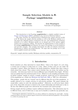


© Copyright 2026