
1 Synchronization of clocks Marcin Kapitaniak1,2, Krzysztof
Synchronization of clocks
Marcin Kapitaniak1,2, Krzysztof Czolczynski1, Przemysław Perlikowski1,
Andrzej Stefanski1, and Tomasz Kapitaniak1*
1
Division of Dynamics, Technical University of Lodz, Stefanowskiego 1/15, 90-924 Lodz,
Poland
2
Centre for Applied Dynamics Research, School of Engineering, University of Aberdeen
AB24 3UE, Aberdeen, Scotland
PACS: 45.40.-f, 05.45.-a
Keywords: synchronization, clocks, discontinuous systems
Abstract: In this report we recall the famous Huygens’ experiment which gave the first
evidence of the synchronization phenomenon. We consider the synchronization of two clocks
which are accurate (show the same time) but have pendulawith different masses. It has been
shown that such clocks hanging on the same beam can show the almost complete (in-phase)
and almost antiphase synchronizations. By almost complete and almost antiphase
synchronization we defined the periodic motion of the pendula in which the phase shift
between the displacements of the pendula is respectively close (but not equal) to 0 or π.We
give evidence that almost antiphase synchronization was the phenomenon observed by
Huygens in XVII century. We support our numerical studies by considering the energy
balance in the system and showing how the energy is transferred between the pendula via
oscillating beam allowing the pendula’s synchronization. Additionally we discuss the
synchronization of a number of different pendulum clocks hanging from a horizontal beam
which can roll on the parallel surface. It has been shown that after a transient, different types
of synchronization between pendula can be observed;(i) the complete synchronization in
which all pendula behave identically, (ii) pendula create three or five clusters of synchronized
pendula. We derive the equations for the estimation of the phase differences between phase
synchronized clusters. The evidence, why other configurations with a different number of
clusters are not observed, is given.
*Corresponding author.
E-mail address: [email protected] (T. Kapitaniak).
1
Contents
1.
Introduction
2.
Pendulum clocks
2.1
Brief history of mechanical clocks
2.2
Escapement mechanisms
2.2.1 Verge-and-foliot escapement
2.2.2 Anchor escapement
2.3
Dynamics of the clock
3.
Modeling Huygens’ experiment: Coupling through elastic structure
3.1
Coupling in Huygens’ experiment
3.2
Senators' five degrees of freedom model
3.3
Model of two double spherical pendula
3.4
Three degrees of freedom discontinuous model
3.4.1 Energy balance of the clocks’ pendula
3.4.2 Energy balance of the beam and whole system (26,27)
3.5
Three degrees of freedom model with van der Pol's friction
3.6
Model with the transversal oscillations of the beam
4.
Synchronization of two pendulum clocks
4.1
Experimental observations
4.2
Numerical results
4.2.1 Synchronization of two identical pendula
4.2.2 Synchronization of two pendula with different masses
4.2.3 Synchronization of two pendula with the different lengths
4.2.4 Chaos in coupled clocks
4.3. Discussion
5.
Synchronization of n clocks
5.1
Experimental synchronization of metronomes
5.2
The model
5.3
Numerical simulations
5.3.1 Identical clocks
5.3.2 Nonidentical clocks
5.4
Discussion
6.
Conclusions
References
Nomenclature
α [rad/s]
-angular frequency of the beam-pendula system oscillations;
αi0 [rad/s]
-angular frequency of i-th pendulum oscillations when the beam is at rest;
βi [rad], [deg] -phase shift between pendula;
βi0 [rad], [deg]-initial value of βi;
βII=β2, βIII=360o-β3,
βIV=β4, βV=360o-β5 [deg]
- phase shift between pendula;
βI0, βII0, βIII0, βIV0, βV0 [deg] - initial values of phase shifts;
δi, σ
- perturbation added to the variables ϕi and x;
γN [rad], [deg] - working angle of the escapement mechanism;
Φi ,Φ [rad] - amplitudes of oscillations of the pendulum;
2
ϕi , ϕ&i , ϕ&&i
ϕi 0 , ϕ&i0
μi
υ [rad]
ξ
A1i, A3i [m/s2]
cϕi [Nsm]
cx [Ns/m]
F1i, F3i [m/s2]
g [m/s2]
H13 [N2]
H15, H35 [N2]
kx [N/m]
l, li [m]
M [kg]
MDi [Nm]
MNi [Nm]
m, mi [kg]
N
T [s]
Ti0 [s]
Ti [s]
Tm [s]
t [s]
U [kg]
DAMP
Wbeam
[Nm]
- displacement [rad], velocity [rad/s] and acceleration [rad/s2] of the i-th
pendulum;
- initial conditions of the i-th pendulum motion;
- mass ratio mi/m1;
- phase shift between the beam and pendulum 1;
- scale factor of the second pendulum (related to the first one);
- amplitudes of first and third harmonical component of the beam acceleration;
- damping coefficient of the i-th pendulum damper;
- damping coefficient of the damper between the beam and the basis; ;
- amplitudes of first and third harmonical component of the force between
pendula and beam;
- gravity;
- square of the amplitude of the first harmonic component of the force acting
on the beam with three pendula;
- square of the amplitude of the first and third harmonic component of the force
acting on the beam with five pendula;
- stiffness coefficient of the spring between the beam and the basis;
- length of the pendulum;
- mass of the beam;
- driven moment equal to 0 or MNi, depending on ϕi and ϕ&i ;
- moment of force generated by escapement mechanism;
- mass of the pendulum;
- number of periods T of pendula oscillations (NT - unit of time);
- period of the beam-pendula system oscillations;
- period of i-th pendulum oscillations when the beam is at rest;
- period of the oscillations of i-th pendulum hanging solo on the moving beam;
- period of long-period synchronization;
- time;
- global mass of the system (beam plus pendula);
- energy dissipated by the beam during one period of motion;
Wi DAMP [Nm] - energy dissipated by the i-th pendulum during one period of motion;
DRIVE
Wbeam
[Nm] - energy delivered to the beam during one period of motion;
Wi DRIVE [Nm] - energy delivered to the i-th pendulum during one period of motion;
Wi VDP [Nm] - energy delivered to the i-th pendulum by van der Pol positive damping during
one period of motion;
SYN
Wi [Nm] - energy delivered from the i-th pendulum to the beam during one period
ofmotion;
X [m]
- amplitude of the beam oscillations;
X1i, X3i [m] - amplitudes of first and third harmonical component of the beam oscillations;
- displacement [m], velocity [m/s] and acceleration [m/s2] of the beam;
x, x& , &x&
x0 , x& 0
- initial values of displacement and velocity of the beam;
3
1. Introduction
A pendulum clock is a clock that uses a pendulum, a swinging weight as its timekeeping
element. The advantage of a pendulum for timekeeping is that it is a resonant device; it
swings back and forth in a precise time interval dependent on its length and resists swinging
at other rates. From its invention in 1656 by Christiaan Huygens(1629-95) until the 1930s, the
pendulum clock was the world's most precise timekeeper, accounting for its widespread use
[7,73,105]. Pendulum clocks must be stationary to operate; any motion or accelerations will
affect the motion of the pendulum, causing inaccuracies.
In the 60-ties of XVII century the longitude problem, i.e., finding a robust, accurate
method of the longitude determination for marine navigation was the outstanding challenge.
Huygens believed that pendulum clocks, suitably modified to withstand the rigors of the sea,
could be sufficiently accurate to reliably determine the longitude1 [97]. In a letter to the Royal
Society of London of 27 February 1665 Huygens described his famous experiment which
showed the tendency of two pendula (of the clocks) to synchronize, or anti-synchronizewhen
mounted together on the same beam [51]. Originally, he usedthe phrase “an odd kind of
sympathy” to describe the observed behavior in two maritime clocks. The original drawing
showing this experiment is shown in Figure 1. Two pendula, mounted together, will always
end up swinging in exactly opposite directions, regardless of their respective individual
motion. This was one of the first observations of the phenomenon of the coupled harmonic
oscillators, which have many applications in physics [89,16,18-20,47,93,5,99], biology and
chemistry [93,60,63,64,100,104]. In engineering very spectacular was synchronization of
pedestrians on Millennium bridge [1,19,36,37,42,81,84,86]. Huygens originally believed the
synchronization occurs due to air currents shared between two pendula, but later after
performing several simple tests he dismissed this and attributed the sympathetic motion of
pendula to imperceptible movement in the beam from which both pendula were suspended.
Figure 1:An original drawing of Huygens illustrating his experimentswith pendulum clocks
Huygens’ study of two clocks operating simultaneously arose from the very practical
requirement of the redundancy: if one clock stopped, had to be cleaned or winded up, then the
other one provided the proper timekeeping [50,53]. Ultimately, the innovation of the
pendulum did not solve the longitude problem, since slight and almost insensible motion was
able to cause an alteration in their work[15,9,21,22].
1
The discrepancy in the clock rate equal to one oscillation of the second pendulum (pendulum with a period of
oscillations equal to 1 [s] in a day corresponds to the error in the longitude determination, approximately equal to
500 m in a day (at the equator).
4
Recently, this idea has been validated by a few groups of researchers who tested
Huygens' idea [11,90,55,96,39,62,43,87,102,31-35]. These studies do not give the definite
answer to the question: what Huygens was able to observe.
To explain Huygens' observations Bennett et al. [11] built an experimental device
consisting of two interacting pendulum clocks hung on a heavy support which was mounted
on a low-friction wheeled cart. The device moves by the action of the reaction forces
generated by the swing of two pendula and the interaction of the clocks occurs due to the
motion of the clocks' base. It has been shown that to repeat Huygens' results high precision
(the precision that Huygens certainly could not achieve) is necessary.
Kanunnikov & Lamper[55] showed that the precise antiphase motion of different
pendula noted by Huygens cannot occur. Different pendula (possibly with different masses)
were definitely used by Huygens as can be seen in his drawing shown in Figure 2.
Pogromsky et al. [90] designed a controller for synchronization problem of two
pendula suspended on an elastically supported rigid beam. A controller solves the
synchronization problem in such a way that the pendula reach the desired level of energy and
they move synchronously in opposite directions. The original Huygens’ problem has been
also related to a practical application of avoiding resonance during the start up procedure of
speeding two unbalanced rotors.
The system very close to the one considered by Huygens (i.e., two pendulum clocks
with cases hanging from the same beam) has been investigated by Senator [96] who
developed a qualitative approximate theory of clocks' synchronization. This theory explicitly
includes the essential nonlinear elements of Huygens’ system, i.e., the escapement
mechanisms but also includes many simplifications.
Figure 2: Details of the Huygens' experiment; it is clearly visible that the clocks used in the
experiment have not been identical, D denotes the weight used to stabilize the clock case.
A device mimicking Huygens' clock experiment, the so-called "coupled pendula of the
Kumamoto University" [62], consists of two pendula which suspension rods are connected by
a weak spring, and one of the pendula is excited by an external rotor. The numerical results of
Fradkov & Andrievsky[43] show simultaneous approximate in-phase and antiphase
synchronization. Both types of synchronization can be obtained for different initial conditions.
5
Additionally, it has been shown that for small difference in the pendula frequencies they may
not synchronize.
A very simple demonstration device was built by Pantaleone[87]. It consists of two
metronomes located on a freely moving light wooden base as shown in Figure 3(a,b). The
base lies on two empty soda cans which smoothly rolls on the table. Both in-phase (Figure
3(b)) and antiphase (Figure 3(a)) synchronization of the metronomes have been observed. The
synchronization problem for larger number of metronomes has been studied inUlrichs et al.
[102]andCzolczynski et al. [31,32].
Figure 3: Synchronization of two metronomes; (a) in-phase synchronization, (b)
antiphase synchronization.
The problem of clocks synchronization is also studied by Blekhman[16] where the
clocks have been modeled as van-der Pol’s type self-excited oscillators (as in [87,102]).
Blekhman also discusses Huygens’ observations, and recounts the results of a laboratory
reproduction of the coupled clocks as well as presenting a theoretical analysis of oscillators
coupled through a common supporting frame. He predicted that both in-phase and anti-phase
motions are stable under the same circumstances.
A synchronous regime in the Huygens' problem is studied byKanunnikov &
Lamper[55]with allowance for nonlinear interaction between the transversal oscillations of a
beam and clock’s pendula. The case where the motion of the pendula is synchronous and
close to the out-of-phase motion is studied.
In this report we repeat Huygens’ experiment using real pendulum clocks. We have
been trying to perform this experiments in the same way as Huygens did them. We hang two
clocks on the same beam and observe the behavior of the pendula. The clocks in the
experiment have been selected in such a way as to be as identical as possible. It has been
observed that when the beam is allowed to move horizontally the clocks can synchronize both
in-phase and anti-phase. As we notice some small differences in the pendulum lengths and
periods (so small to be identified in the Huygens’ time) we perform computer simulations to
answer the question: how the nonidentity of the clocks influences the synchronization process.
We show that even the clocks with significantly different periods of oscillations can
synchronize, but their periods are modified by the beam motion so they are obviously no more
accurate.
This review paper is organized as follows. Section 2 briefly describes the history of
mechanical clocks. The clock mechanisms necessary for the compensation of the energy
dissipation due to friction [94,95,67,8] are described. In Sec. 3 we describe the coupling
through elastic structure and explain why this type of coupling is different from other types
used in the network synchronization schemes. The main Section 4 recalls original Huygens
experiment and discusses the synchronization of two clocks. We give explanation why and
6
under which conditions two clocks can synchronize. We discuss the possibility of the chaotic
behavior in pendulum clocks [77]. Sec. 5 describesthe behavior of more than two coupled
clocks. We present the results ofthe numerical studies and the experimental visualization of
different types of synchronization. We give theoretical explanation of the existence of only
three or five clusters of the synchronized pendula[31,32]. Later, we discuss the influence of
the parameter mismatch on the behavior of the system [35].Finally, we summarize our results
in Sec. 6.
2. Pendulum clocks
2.1. Brief history of mechanical clocks
In the early-to-mid-14th century, large mechanical clocks began to appear in the
towers of several large Italian cities. These clocks were weight-driven and regulated by a
verge-and-foliot escapement [95]. This mechanism pre-dates the pendulum and was originally
controlled by a foliot, a horizontal bar with a weight at each end [45] (the details of this
mechanism design are given in Sec. 2.2).
Figure 4: (a) The first pendulum clock, invented by Christiaan Huygens in 1656, (b) . The
second verge pendulum clock built in 1673.
A significant advance was the invention of spring-powered clocks between 1500 and
1510 by a German locksmith Peter Henlein [73]. Replacing the heavy drive weights permitted
the smaller clocks. Although they slowed down as the mainspring unwound, they were
popular among wealthy individuals due to their size and the fact that they could be put on a
shelf or table instead of hanging from the wall.
7
The pendulum clock was invented in 1656 by Ch. Huygens, and patented the
following year [26]. The sketches of the first two designs of the pendulum clocks are shown
in Figure 4(a,b). Huygens was inspired by investigations of pendula by Galileo Galilei
beginning around 1602. Galileo discovered the key property that makes the pendulathe useful
timekeepers, i.e., isochronism, which means that the period of swing of a pendulum is
approximately the same for different sized swings [49]. He designed the pendulum clock
shown in Figure 5, but there are no evidences that it has ever been built. The introduction of
the pendulum, the first harmonic oscillator used in timekeeping, increased the accuracy of the
clocks enormously, from about 15 minutes per day to 15 seconds per day
[6,38,46,48,76,77,80,95] leading to their rapid spread as the existing 'verge and foliot' clocks
were retrofitted with pendula.
Figure 5: Pendulum clock conceived by Galileo Galilei around 1637. The earliest known
pendulum clock design, it was never completed.
These early clocks, due to their verge escapements, had wide pendulum swings of up
to 100 . Huygens discovered that wide swings made the pendulum inaccurate, causing its
period, and thus the rate of the clock to vary with unavoidable variations in the driving force
provided by the movement [50,53]. The observation that only the pendula with small swings
of a few degrees are isochronous motivated the invention of the anchor escapement around
1670, which reduced the pendulum's swing to 4o-6o [95]. In addition to the increased
accuracy, this allowed the clock's case to accommodate longer, slower pendula, which needed
less power and caused less wear on the movement.
o
To summarize the description, all mechanical pendulum clocks have five basis parts as
shown in Figure 6, i.e.:
8
Figure 6:The sketch of the basic components of a pendulum clock with anchor escapement.
(after [70]: (1) pendulum; (2) anchor escapement arms; (3) escape wheel; (4–7) gear train; (8)
gravity-driven weight; (9-11) energy supply mechanism, (12-14) transition mechanism,
(15,16) clock’s hands.
(i) a power source; either a weight on a cord that turns a pulley, or a spring, (ii) a gear train
that steps up the speed of the power so that the pendulum can use it, (iii) an escapement that
controls the speed and regularity of the pendulum. It transfers the energy stored in the spring
to the motion of the pendulum by means of wheels, gears, and ratchets, i.e., it gives the
pendulum precisely timed impulses to keep it swinging, and which releases the gear train
wheels to move forward a fixed amount at each swing, (iv) the pendulum, a weight on a rod,
(v) an indicator or a dial that records how often the escapement has rotated and therefore how
much time has passed, usually a traditional clock face with rotating hands.
2.2.Escapement mechanisms
An escapement transfers energy to the clock's timekeeping element (usually a
pendulum or foliot) to compensate the energy dissipation during a cycle as without the energy
transfer, the oscillation of the pendulum (foliot) will decay [88]. The escapement may take the
energy from a coiled spring or suspended weight [83]. The escapement also permits each
cycle of the timekeeping element to be counted. During each cycle, the escapement permits a
gear train to advance or "escape" slightly. The periodic advancement results in moving the
timepiece's hands forward at a steady rate.
With each swing of the pendulum, one of its arms releases one tooth of a gear, making
it change from a "locked" state to a "drive" state for a short period that ends when another
tooth on the gear strikes the opposite arm of the pendulum, which locks the gear again. It is
9
this periodic release of energy and rapid stopping that makes a clock "tick;" it is the sound of
the gear train suddenly stopping when the escapement locks again.
The invention of the escapement mechanism has a significant influence on the history
of technology as it made the all-mechanical clock possible [73,48]. This development in 13th
century Europe initiated a change in timekeeping methods from continuous processes, such as
the flow of water in water clocks, to repetitive oscillatory processes, such as the swing of
pendula, which could yield more accuracy [27,68,103].
Greek washstand automaton of the 3rd century BC is the earliest known example of an
escapement mechanism [63]. The earliest liquid-driven escapement was described by the
Greek engineer Philo of Byzantium (3rd century BC) in his technical treatise Pneumatics
(chapter 31) as part of a washstand. A counterweighted spoon, supplied by a water tank, tips
over in a basin when full, releasing a spherical piece of pumice in the process. Once the spoon
has emptied, it is pulled up again by the counterweight, closing the door on the pumice by the
tightening string. Philo's comment that "its construction is similar to that of clocks" indicates
that such escapement mechanisms were already used in ancient water clocks [63].
In China around 723 AD, during the period of theTang Dynasty Buddhist monk Yi
Xing along with government official Liang Lingzan applied the escapement in the waterpowered armillary sphere and clock drive [82]. The Song Dynasty (960–1279) era horologists
Zhang Sixun and Su Song (1020–1101) duly applied escapement devices in their astronomical
clock towers [82,41].
Amercury escapement mechanism has been described in the work of the king of
Castile Alfonso X. The knowledge of these mercury escapements may have spread through
Europe with translations of Arabic and Spanish texts [3].
None of these were true mechanical escapements, since they still depended on the flow
of liquid through an orifice to measure time. For example, in Su Song's clock water flowed
into a container on a pivot. The escapement role was to tip the container over each time it
filled up, thus advancing the clock's wheels each time an equal quantity of water was
measured out.
The first mechanical escapement is the verge-and-foliot mechanism invented by
Villard de Honnecourt in XIV century Europe.It was a primitive apparatus that was
apparently a timekeeping device, but without being subject to any minute requirement of
accuracy [48].It was used in a bell ringing apparatus called an alarum for several centuries
before it was adapted to clocks [103]. In 14th century Europe it appeared as the timekeeper in
the first mechanical clocks, which were large tower clocks. Its origin and first use is unknown
because it is difficult to distinguish which of these early tower clocks were mechanical, and
which were water clocks. However, indirect evidence, such as a sudden increase in cost and
construction of clocks, points to the late 13th century as the most likely date for the
development of the modern clock escapement. The astronomer Robertus Anglicus wrote in
1271 that clockmakers were trying to invent an escapement, but hadn't been successful yet
[85].
On the other hand, most sources agree that mechanical escapement clocks existed by
1300. The earliest description of the mechanical escapement can be found in Richard of
Wallingford's manuscript Tractatus Horologii Astronomiciof 1327 AD, on the clock he built
at the Abbey of St. Albans. (Jones, 2000, Dohrn-van Rossum, 1996). It consisted of a pair of
escape wheels on the same axle, with alternating radial teeth. The verge rod was suspended
between them, with a short crosspiece that rotated first in one direction and then the other as
the staggered teeth pushed past.
Unlike the continuous flow of water in the Chinese device, the European medieval
escapements were characterized by a regular, repeating sequence of discrete actions and the
10
capability of self-reversing action. Both techniques used escapements, but these have only the
name in common. The Chinese one worked intermittently; the European, in discrete but
continuous beats. Both systems used gravity as the prime mover, but the action was very
different. In the mechanical clock, the falling weight exerted a continuous and even force on
the train, which the escapement alternately held back and released at a rhythm constrained by
the controller. Ingeniously, the very force that turned the scape wheel then slowed it and
pushed it part of the way back. In other words, a unidirectional force produced a selfreversing action—about one step back for three steps forward. In the Chinese timekeeper,
however, the force exerted varied, the weight in each successive bucket increases until it is
sufficient to tip the release and lift the stop that held the wheel in place. This allowed the
wheel to turn some ten degrees and bring the next bucket under the stream of water while the
stop fell back. In the Chinese clock, then unidirectional force produced unidirectional motion
[66].
The verge-and-foliot was the standard escapement used in every other early clock and
watch and remained the only escapement for 400 years [44]. Its friction and recoil limited its
performance but the accuracy of these 'verge-and-foliot' clocks was more limited by their
early foliot type balance wheels, which because they lacked a balance spring had no natural
'beat', so there was not much incentive to improve the escapement [17].
The great leap in accuracy resulting from the invention of the pendulum and balance
spring around 1657, which made the timekeeping elements in both watches and clocks
harmonic oscillators, focused attention on the errors of the escapement and more accurate
escapements soon superseded the verge. The next two centuries, the 'golden age' of
mechanical horology, saw the invention of perhaps 300 escapement designs [21,22,24,25],
although only about 10 stood the test of time and were widely used [54]. The reliability of an
escapement depends on the quality of workmanship and the level of maintenance given [91].
A poorly constructed or poorly maintained escapement will cause problems. The escapement
must accurately convert the oscillations of the pendulum or balance wheel into rotation of the
clock or watch gear train, and it must deliver enough energy to the pendulum or balance
wheel to maintain its oscillation.The most accurate commercially produced mechanical clock
was the Shortt-Synchronome free pendulum clock invented by W. H. Shortt in 1921, which
had an error rate of about 1 second per year [54].
Now, let’s describe in more details two most commonly used escapement
mechanisms.
2.2.1. Verge-and-foliot escapement
The earliest escapement in Europe (from about 1275) was the verge escapement, also known
as the crown-wheel escapement. It was used in the first mechanical clocks and was originally
controlled by a foliot, a horizontal bar with weights at either end. The sketch of the verge-andfoliot mechanism is shown in Figure 7. A vertical shaft (verge) is attached to the middle of the
foliot and carries two small plates (pallets) sticking out like flags from a flag pole. One pallet
is near the top of the verge and one near the bottom and looking end-on down the verge the
pallets are a little over ninety degrees apart. The escape wheel is shaped somewhat like a
crown and turns about a horizontal axis. The mechanism is driven by a constant torque τ
applied to the crown gear. This torque is usually provided by a mass hanging from a rope
which is wound around the shaft. The verge spins freely at all times except at the instant a
collision takes place. Energy is assumed to leave the system only through the collisions. The
11
amount of energy lost during each collision is a function of the system geometry as well as the
coefficient of restitution realized in the collision [94]. As the wheel tries to turn, one tooth of
the wheel pushes against the upper pallet and starts the foliot moving. As the tooth pushes
past the upper pallet, the lower pallet swings into the path of the escape wheel. The
momentum of the moving foliot pushes the escape wheel backwards but eventually the system
comes to rest. It is now the turn of the lower pallet to push the foliot and so on. The system
has no natural frequency of oscillation - it is simply force pushing inertia around. Verge-andfoliot mechanisms reigned for more than 300 years with variations in the shape of the foliot.
All had the same basic problem: the period of oscillation of this escapement depended heavily
on the amount of driving force and the amount of friction in the drive and was difficult to
regulate.
Figure 7: Verge-and-foliot escapement mechanism (after [94]).
A disadvantage of the escapement was that each time a tooth lands on a pallet, the momentum
of the foliot pushes the crown wheel backwards a short distance before the force of the wheel
reverses the motion. This is called "recoil" and was a source of wear and inaccuracy.
Let the crown gear and the verge have inertias Ic and Iv , contact radii rc and rv, and
angular velocities
,
, respectively. The velocities before and after a collision
are denoted by the subscripts 0 and 1, respectively. The motion of the crown gear and verge is
governed by the equations
,
,
,
(1)
,
,
,
,
upper
,
,
,
,
lower
(2)
where the first expression in eq. (2) applies to the collisions between the crown gear and the
upper paddle, and the second expression applies to the collisions between the crown gear and
the lower paddle. The function
,
,
,
is the collision force, which is
zero when the crown gear and verge are not in contact and is impulsive at the instant of
12
impact. The collision force F acts equally and oppositely on the crown gear and verge. Let's
define
1, upper
1, lower
(3)
and rewrite eq. (2) in the following form
,
,
,
.
(4)
To determine the collision force, one can integrate eqs (1) and (4) across a collision, i.e.,
limΔ
limΔ
Δ
Δ
Δ
Δ
Δ
Δ
.
(5)
(6)
Eliminating the integrated collision force in eqs (5) and (6) yields
(7)
which is an expression of conservation of linear momentum at the instant of a collision. Eq.
(7) can be rewritten as
(8)
where Mc=Ic/rc2 and Mv=Iv/rv2 are the effective crown gear mass and effective verge mass,
respectively, and Vc and Vv are the tangential velocities of the crown gear and the verge,
respectively
,
.
The coefficient of restitution e relates the linear velocities of the crown gear and the
verge before and after the collision according to
(9)
which accounts for the loss of kinetic energy in a collision. Solving eqs (7) and (9) yields
Δ
(10)
Δ
(11)
whereΔ
,Δ
are the impulsive changes in angular velocity when a
collision occurs. These quantities depend on the geometry as well as the velocities
immediately before the collision. The integral of the impulsive force function over a collision
event is
(12)
where t0 is time slightly before the collision and t1 is time slightly after the collision
13
The verge was the only escapement used in clocks and watches for 400 years. It was
used in the first pendulum clocks for about 50 years after the pendulum clock was invented in
1656. In a pendulum clock the crown wheel and verge were oriented so they were horizontal,
and the pendulum hung from the verge. However the verge is the most inaccurate of the
common escapements, and after modern timekeeping oscillators (the pendulum and the
sprung balance wheel) were introduced in the 1650s the verge was replaced by other
escapements [2].
2.2.2. Anchor escapement
The anchor escapement mechanism shown in Figure 8 was invented by Robert Hooke around
1660, the anchor quickly superseded the verge to become the standard escapement used in
pendulum clocks through the 19th century. Its advantage was that it reduced the wide
pendulum swing angles of the verge to 3°-6°, making the pendulum isochronous, and
allowing the use of longer, slower moving pendula, which used less energy. It is responsible
for the long narrow shape of most pendulum clocks.
Figure 8: Anchor escapement.
It consists of an escape wheel with pointed, backward slanted teeth, and an 'anchor'
shaped piece pivoted above it which rocks from side to side, attached to the pendulum. The
anchor has slanted pallets on the arms which alternately catch on the teeth of the escape
wheel, receiving impulses. Mechanically its operation has similarities to the verge
escapement, and it has two of the verge's disadvantages: (1) The pendulum is constantly being
pushed by an escape wheel tooth throughout its cycle, and is never allowed to swing freely,
which disturbs its isochronism, and (2) it is a recoil escapement; the anchor pushes the escape
wheel backward during part of its cycle. This causes a backlash, an increased wear in the
clocks gears, and inaccuracy. These problems were eliminated in the deadbeat escapement,
which slowly replaced the anchor in precision clocks.
14
Figure 9: Deadbeat escapementmechanism.
The deadbeat escapement of Figure 9 was an improvement of the anchor escapement
first made by Thomas Tompion to a design by Richard Towneley in 1675 although it is often
credited to Tompion's successor George Graham who popularized it in 1715 [95,48]. In the
anchor escapement the swing of the pendulum pushes the escape wheel backward during part
of its cycle. This 'recoil' disturbs the motion of the pendulum, causing inaccuracy, and
reverses the direction of the gear train, causing backlash and introducing high loads into the
system, leading to friction and wear. The main advantage of the deadbeat is that it eliminated
a recoil [103].
In the deadbeat, the pallets have a second curved "locking" face on them, concentric
about the pivot the anchor turns on. During the extremities of the pendulum's swing, the
escape wheel tooth rests against this locking face, providing no impulse to the pendulum,
which prevents the recoil. Near the bottom of the pendulum's swing the tooth slides off the
locking face onto the angled "impulse" face, giving the pendulum a push, before the pallet
releases the tooth. This was the first escapement to separate the locking and impulse actions
of the escapement. The deadbeat was first used in precision regulator clocks, but due to
greater accuracy superseded the anchor in the 19th century. It is used in almost all modern
pendulum clocks.
Now let’s describe the dynamics of a typical anchor mechanism as shown in Figure
10(a-c).
15
Figure 10: Anchor escapement mechanism; (a) scheme of the mechanism, (b) view of the
scape wheel, (c) view of the anchor pallets.
16
Figure 11. Acting of
o the escap
pement mecchanism.
m
c
consists
of the scape wheel
w
(detaiils are show
wn in Figurre 10(b))
The esccapement mechanism
and twoo anchor palllets mounteed on the peendulum axis (details are
a shown inn Figure 10((c)). The
energy is suppliedd by a wouund spring connected with the scape
s
wheeel. The escapement
F
11(a-d). In the first
f
stage one
o of the trriangle shap
ped teeth
mechannism acts as shown in Figure
of the scape
s
wheell impacts thhe pallet I. For
F the ang
gle of penduulum displaacement φ<0
0(Figure
11(a)) surface
s
A of
o the pallett I slides onn the top ed
dge of the triangle teeeth 1 and ex
xcitation
momentt M=0. In thhe case of 0<φ<γ
0
) the edge of
o the pallet I is in conttact with
N (Figure 11(b))
the sidee surface of
o the teethh 1 and thhe horizontal componeent of the reaction generates
g
excitatioon moment MN. Whenn increasing φpasses criitical value γ, pallet I sslides off thee teeth 1
and the second stagge of the mechanism
m
a
acting
startss. The teeth 1 impacts oon the palleet II. For
o the pallett II slides on the edge of
o the teeth 1 and no ex
xcitation
φ>0 (Fiigure 11(c))) surface B of
momentt is generateed. When -γγN<φ<0 (Fiigure 11(d) the edge off the pallet III is in conttact with
the sidee surface of
o the teethh 1 and thhe horizontal componeent of the reaction generates
g
excitatioon momentt -MN. Whenn φ exceedss the criticaal value -γN, i.e., φ<-γN the pallet II slides
off the teeth 1. Neext, the succcessive teetth 2 impacts pallet I annd the first stage startts again.
Notice that
t
when maximum
m
a
absolute
vallue of φ is smaller
s
thann γNtheescaapement meechanism
does noot work (thee transition from step I to step II is impossibble) and the pendulum tends to
the equiilibrium possition φ=0.
17
2.3. Dynamics of clocks
The pendulum clock is an oscillatory mechanism with self-excited oscillations whose
amplitude is independent of the initial conditions (dynamical system has a stable limit cycle
attractor [12,58,59]. To start the oscillations a rather strong initial impulse is required; failing
this the clock goes back to rest, i.e., dynamical system has an additional fixed point attractor
which is obtained for the initial conditions close to zero. For certain positions of the pendulum
the control operates and allows the required energy to pass in the form of an impulse
[71,13,14]. The duration of the impulse varies from clock to clock, but in the good clocks it is
quite short. The control operates generally twice per period, close to the position of
equilibrium, i.e. where the velocity is the greatest. An important feature is that the moment
when the control operates depends solely on the position of the pendulum. Furthermore its
action, and notably the magnitude of the impulse, depends on the state of the pendulum.
Hence the whole operation depends on the position and velocity of the parts and not on time.
Thus a clock is an autonomous system [8]. The main properties of the clock’s model are
summarized in Figure 12. The initial conditions starting in the shaded region after a finite
number of pendulum’s oscillations lead to the equilibrium (0,0), while these starting in the
rest of the plane tend to the limit cycle (shown in red).
Figure 12. An autonomous model of the clock.
For simplicity, we can assume that the control acts once in each period of the pendulum,
producing an instantaneous change in velocity. One can consider two "laws of impulse", one
asserting that the change in velocity is constant, the other that the change in kinetic energy is
constant, i.e., if v0 and v1 are the velocities of the pendulum just before and after the impulse,
the first states that mv1-mvo= constant, the second that mv12-mv02=constant. The second is very
natural since it holds exactly when the unwinding mechanism consists of a weight which is
displaced downward the same distance (thus doing the same work) in each period. Of the two
assumptions, the second is more plausible since it asserts that each impulse contributes the
same amount of energy. The first assumption may imply a larger change of energy for some
impulses than for others; the lower the velocity before the impulse the less energy transferred
to the system. In addition to the nature of the impulse there are also hypotheses to be made
regarding friction. The simplest are: (a) linear friction, or friction proportional to the velocity;
(b) constant friction. The friction in an actual clock is partly of a constant type, as in that of
control and partly variable, as in that from the air resistance of the pendulum. Constant
friction is related to the property of soft self-excitation and the necessity of a strong impulse
to start the periodic limit cycle oscillations. In [8] one can find the proof that the model
18
considering the second impulse law and a combination of both types of friction can exhibit a
limit cycle behavior and capture the main properties of the clocks.
(i)
Discontinuous model
The equation of motion of the clock’s pendulum is as follows:
ml 2ϕ&& + cϕϕ& + m gl sin ϕ = M D ,
(13)
where MD is the momentum supplied by the escapement mechanism (see Sec. 3.2), i.e., in the
first stage if 0<ϕ<γN then MD=MN and when ϕ<0 then MD=0 and for the second stage one has
for -γN<ϕ<0 MD=-MN and for ϕ>0 MD=0. When max |φ(t)|<γN there are switches between two
stages and MN=0. Eq. (13) describes the dynamical system which performs the self-excited
oscillations [8].
The clocks are designed in such a way that the pendula perform periodic motion with a
period 2π/α where α is constant. The escapement mechanism provides the necessary amount
of energy to compensate the dissipation and makes the pendulum motion periodic. Under
these assumption in the stable motion of the clock’s pendula has been approximated by:
ϕ = Φ sin(αt ),
(14)
where Φ is constant. The continuous solution given by eq. (14) is a good approximation of the
pendula’ oscillations calculated from discontinuous eq. (13) as can be seen in Figure 13. A
stable limit cycle calculated from eq.(13) is shown in blue while the approximation given by
eq.(14) is shown in red. Notice that for initial conditions -γN<φ0<γN,-αγN <γN eq.(13) has a
stable fixed point attractor at (0,0).
Figure 13. Comparison of the numerical solution of discontinuous eq. (13) with the harmonic
assumption (14).
Typically pendulum clocks oscillate with amplitude smaller than 2π/36 and for clocks with
long pendula like marine clocks this amplitude is even smaller [95].
(ii)
Moon’s model
In a series of papers[76,77,80], the following mathematical model has been considered. It
involves the impact as a generic model designed to capture the essential features for chaos in
clocks.
The model incorporates the following assumptions and features: (i) the pendulum is
modelled by a linear harmonic oscillator with light damping,(ii) the impact dynamics in the
19
escapement and the propagation of structural dynamics through bearings with gaps is
modelled by a cubic oscillator of the Duffing-type coupled linearly [75,78,79] to the
pendulum equation,(iii) the driving gear train torque and static friction lock-up are modelled
by a threshold condition of structural impact velocity as measured by the Duffing oscillator,
and(iv) the driving torque from the weight-driven gear train, when released by the Duffing
oscillator noise, acts to add energy through the escapement pallet when the pendulum velocity
is positive.
The first assumption (i) is based on the fact that the pendula in clocks rotate through a
very small amplitude such that the nonlinear effects are not important [56,18]. The linear
oscillator assumption is also good for balance wheel clocks. The second assumption (ii) is
motivated by the research on the propagation of stress waves in structures. Both the
experimental and the theoretical research show that a single impact or a step input load on a
structure leads to complex wave patterns through reflections and dispersions which excite
many modes in the structure. Thus, the escapement impact energy redistribution can
propagate into the gear train, break the friction and prevent the lock-up. These assumptions
lead to the following equations of motion for the coupled pendulum, structural dynamics and
driving train. This fourth-order model employs a vibration-sensitive torque to capture the
escapement impact:
(15)
0
(16)
where
if
and 0
Δ
0 otherwise.
Here x1(t) represents the motion of the pendulum or balance wheel oscillator; x3(t) represents
the motion of the structural connection between the escapement and the driving train; the
cubic term is a nonlinear surrogate for the gaps between bearings and gear teeth. The torque
dependence on structural velocity is an attempt to capture the static friction in the drive train
and its dependence on the structural vibration.
The frequency ω1 represents the regular motion of the clock oscillator. The damping
constants β1 and β2 measure the oscillator and structural damping, respectively. The
escapement torque is only applied when the amplitude is in a given sector of the phase space,
e.g. 0<x1<Δ. Thus, Δshould be a small fraction of the limit cycle amplitude. In addition, the
noise threshold to release the gears and apply the escapement torque is measured by constant
δ.
To ensure that the model does not generate vibrations when the impact torque tq is
zero, an energy function can be constructed that places restrictions on the constants in the
above model. Multiplying the first equation above by α2(dx1/dt), the second equation by
α1(dx2/dt) and adding, one comes up with the following energy equation:
(17)
where
20
1
2
1
2
1
4
2
Here T acts like a kinetic energy function and V like the potential energy function. To ensure
energy decay when tq=0, both α1 and α2 must be positive as well as the nonlinear stiffness
constant, k. When the torque is active, the product, tq(dx1/dt),must be also be positive, thus the
reason for appearance of the sign(dx1/dt) function in the model.
(iii)
Impulsive differential equations’ model
In this section we describe the equations of motion of the escapement mechanism in the form
of an impulsive differential equation [10,65,94]. An impulsive differential equation is
described by three components; namely, a continuous time differential equation, which
governs the system state between the impulses, an impulse equation, which models an
impulsive jump defined by a jump function at the instant an impulse occurs, and a jump
criterion, which defines a set of jump events in which the impulse equation is active. These
components can be written in the form
, (18)
Δ
, (19)
where t≥0, x ϵ Rn, fc:Rn →Rn is locally Lipschitz continuous; fd:Rn →Rn is continuous; and S
\in Rn is the jump set. Eqs. (18) and (19) describe the impulsive dynamical system G.
The dynamics of the verge and foliot escapement mechanism as an impulsive
differential equation define the state
, , ,
, , ,
(20)
where x1 is the position of the crown gear, that is, the counterclockwise angle swept by the
line connecting the centre of the crown gear and the 0-th tooth from the 12 o’clock position;
x2 is the position of the verge, that is, the deviation of the mean line of the angular offset
between two paddles from the vertical plane perpendicular to the plane of the crown gear; x3
is the angular velocity of the crown gear; and x4 is the angular velocity of the verge. Between
collisions the state satisfies
0
0 0 1 0
0
0 0 0 1
1
0 0 0 0
0 0 0 0
0
while the jump function is given by
0 0
0 0
0 0
0 0
0
0
0
0
where
/
/
The jump set is
21
1
/
, /
/
1
/
where, for m=0,…,n
:
sin
tan
0,
2
1/2
/2 ,
1/2
2
,
0,1,2, …
:
sin
tan
0,
2
1/2
1
/2 ,
1/2
2
1
,
0,1,2, …
where αc is the angle between neighboring teeth on the crown gear, αv is the angular offset of
the paddles about the vertical axis, m is the index of the crown gear tooth involved in the
collision and p is the number of full rotations of the crown gear. The crown gear teeth are
numbered from 0 to n clockwise, or opposite the direction of increasing θc, beginning at θc=0.
There must be an odd number of crown gear teeth for the mechanism to function correctly,
and thus n is even.
(iv)
Continuous model with van der Pol’s damping
Instead of the models with an impulse supply of energy to the clock pendulum (i-iii), a van
der Pol oscillator model with a continuous supply of energy can be considered [74,18,87,102].
In this case the equation of motion of a single pendulum clock is as follows,
.
.
sin
1
0
(21)
where θ is the angle the pendulum makes with the vertical, I is the moment of inertia of the
pendulum, m is the mass ofthe pendulum, rc.m. is the distance of the pendulum’s center of
mass from the pivot point, g is the acceleration of gravity,and x is the horizontal position of
the base. The first twoterms in eq.(21) are the usual ones that describe the motionof a
pendulum, that is, the angular acceleration and the gravitationaltorque. The third term in Eq.
(21) crudely models the escapement mechanism and any damping of the bob’smotion from air
resistance. This term is of van der Pol’stype and increases the angular velocity for θ<θ0 and
decreasesit for θ>θ0. For small є, this term will producestable oscillations with an amplitude
of approximately 2θ0 inthe isolated oscillator.
22
3. Modeling Huygens' experiment: Coupling through elastic structure
3.1 Coupling in Huygens’ experiment
In his letters Huygens limited himself to explaining the observed phenomenon of
synchronization by describing the setup (as shown in Figure 1-2), noting the basic coupling
mechanism, and describing how a steady synchronized state is approached. Huygens
originally thought the coupling was due to imperceptible air-borne forces transmitted between
the pendula of the two clocks (letter to his father [51]), but within a few days he realized
(letter to Moray [51]) that the coupling was due to structure-based forces. Huygens’ published
explanation can be summarized in the following way: the common beam [53] or the two
coupled beams [51] from which the extended clock cases are suspended can move (oscillate)
horizontally, at least with small amplitudes. The two pendula, oscillating in the same (or
parallel planes), transmit through their pivots the oscillating forces on two clock-cases,
which, in turn, transmit through their pivots the oscillating forces on the beams which cause
them to oscillate. Only in the case of the two pendula which started in ideal opposition, the
zero resultant oscillating force on the beams causes the beams to stay in the equilibrium
position. As the two nearly identical clocks initially run at slightly different speeds their
pendula eventually get in opposition, two oscillating force components almost completely
cancel, and the motion of the beams goes to zero. Then two clocks adjust their speeds, and
their pendula remain in opposition. Huygens had noted two basic features of his setup—the
clocks adjusting their speeds to common speed (Huygens’ two clocks, when running
independently, differed by daily average times that ranged from -0.5 to 6 [s] [53]; and the
structure-based origin of the coupling forces.
This type of coupling is different from the one used in the most studies of the coupled
oscillatory systems or coupled networks (e.g., [18-20,69,89]) where the signal from one of the
oscillators (network nodes) is transmitted directly to few (or all) of other oscillators and
influence its behavior. If the particular oscillator is n dimensional the dimension of the
coupled system (network) is equal to Nn, where N is a number of oscillators coupled in the
considered system. In the Huygens type coupling the oscillators are coupled to the additional
M dimensional dynamical system B. The signals from the oscillators are transferred to system
B and influence its dynamical behavior. Simultaneously, the signals from system B are
transmitted to the oscillators also changing its dynamics. The transfer of any signal from one
oscillator to another occurs always through the system B. In the consideration of the dynamics
of the coupled system one has to consider Nn+M dimensional model. As in the mechanical
systems (like Huygens’ setup) this additional system B is usually an elastic structure. We call
this type of coupling as the coupling through elastic structure [28-30]. Later in this section
and Sec. 4 we describe how the energy is transferred from one clock to another via the beam.
The studies of the dynamics of the systems coupled through the elastic structure have
been also stimulated by the events on the Millennium Bridge. On the opening day the
Millennium Bridge, a pedestrian footbridge crossing the Thames River in London, was
observed to exhibit a pronounced lateral wobbling as more and more people streamed onto the
bridge [36,37,81,42,92,101,1]. This phenomenon apparently occurred due to a resonance
between a low order bridge oscillation mode and the natural average stepping frequency of
human walkers: a small initial oscillation of the bridge induces some of the walkers to
synchronize the timing of their steps to that of the bridge oscillations, thus exerting a positive
feedback force on the bridge that derives the bridge oscillation to higher amplitude, eventually
resulting in a large steady-state oscillation. Subsequent studies by the bridge builder showed
that the oscillations did not develop unless the number of the pedestrians on the bridge was
greater than a critical value [36,37]. Generally, the phenomenon on the Millennium Bridge
can be considered as a particularly dramatic example of the emergence of global collective
23
behavior in the systems of many coupled heterogeneous oscillators [100]. The examples of
this general type of emergent behavior are known in biology (e.g. synchronization of
pacemaker cells in the heart [72] and of neurons governing day-night rhythms in mammals
[104,5], chemistry [60]).
The analysis of the coupled periodic oscillators can be based on Malkin’s theorem
[16,106,107]. It gives general conditions under which weakly connected periodic oscillators
can be reduced to the analysis of the corresponding phase model. Recently, this approach has
allowed the derivation of a number of important results, mainly on the Kuramoto model
[105]. The discontinuity of the clock model does not allow the application of this method in
most of our models. In the case of continuous model (eqs (68,69) in Sec. 3.5) the analysis
based on Malkin’s theorem will be reduced to the analysis of coupled van der Pol’s oscillator
presented in [105].
3.2 Senators' five degrees of freedom model
Korteweg studies [61] gave further explanations of Huygens’ observed phenomena. He
developed a dissipationless, three-degree-of-freedom, linear model that represents some
features of the original setup of Figure 1 (his model is essentially equivalent to the one formed
from the five-body (two clocks cases, two pendula and a beam) system shown in Figure 1 by
clamping each extended clock-case to its support beam, removing all friction, and removing
the escapements). Korteweg then investigated how the observed natural frequencies and mode
shapes would vary as model’s parameters vary, and used his study results to make the
hypothesis that explained the observed behavior of Huygens’ real system. Korteweg’s basic
idea can be summarized as follows: the stable, steady-state motions of the real, nonlinear, two
coupled clock system can be approximately represented by his model vibrating in one of its
normal modes at the corresponding natural frequency. The approximating mode and its
frequency are found by; (i) adding linear friction to the model, (realistically assuming that the
pendulum friction is extremely small while the beam-motion friction is small), (ii)
determining the exponentially-damped oscillating modes of the lightly damped linear model
which persist the longest and (iii) identifying the undamped normal mode that most closely
approximates this persisting damped mode. It was found that the undamped mode
corresponding to the persisting damped mode would have a frequency between the
frequencies of the two pendula (oscillating independently from fixed pivots) and a mode
shape with the pendula moving in opposition to each other. Korteweg studies showed that the
actual nonlinear system’s motion would be approximately like a modal motion of a related
dissipationless linear system having similar inertial and stiffness properties; and that relative
friction magnitudes would determine which mode would be the approximating one [96].
Following the path of Korteweg Senator [96] developed a five degrees of freedom
model shown in Figure 14. The aim of his study was to develop simple intuitive approximate
theory that would explain the observed clocks' synchronizations. The developed theory
considers the essential nonlinearities and discontinuities of the system, i.e., the impulsive
acting of the escapements; allows consideration of non-identical clocks; and explicitly
includes the suspended clock-case feature of Huygens’ setup.
In addition to forming and analyzing the related dissipationless and damped-linear
systems having the same inertial/stiffness/(damping) properties as the original nonlinear
system, other related systems are also formed and analyzed. These include the related
dissipationless nonlinear systems having the same inertial/stiffness/escapement properties as
the original systems, and the related constrained single-degree-of-freedom nonlinear systems
formed from the original systems by adding judiciously chosen rigid, massless, frictionless
linear constraints. When the generalized constraining (reaction) forces/impulses of these
systems are small, the necessarily proportional steady-state motions of these constrained
24
systemss are expeccted to acccurately appproximate the
t steady--state motioons of the original
intractabble nonlineaar systems.
Figurre 14: Senattor's model of the Huyg
gens experim
ment (after [96]).
Senator's appproach is based
S
b
on thhree main siimplificatioons. One sim
mplification
n used is
to ignorre all large amplitude
a
p
pendula'
osccillations, so
o the angless between thhe pendula and
a their
vertical equilibrium
m positions and the rattes of chang
ge of these angles are assumed to
o always
remain small. The second sim
mplification is to lineariize all damppers (frictioon based disssipative
ures two esssential feaatures of th
he actual
elementts). This linnear frictioon simplificcation captu
friction in the Huyygens experriment, i.e., that at inttermediate and high vvelocity amp
plitudes,
friction forces inccrease as velocity
v
maagnitude inccreases, annd, for suitably small friction
25
parameter magnitudes, that cyclic energy dissipated is small in comparison to the energy that
is cyclically converted between potential and kinetic forms. The third simplification is
connected with the modeling of the nonlinear energy resupply features of the escapement
mechanism. Huygens’ pendulum clocks used a almost-400-year-old verge-and crown-wheel
escapement design (see Figure 7 and Sec. 2.2.1) for which Senator used the constant-impulsemagnitude escapement model of Andronov et al. [8]. For this model, at two opposite points in
the pendulum displacement cycle, a crown-wheel tooth hits a pallet (the escapement fires),
and a constant magnitude impulse is applied between a rigid body having the effective inertia
of the pendulum at the pitch radius of the impact, and a rigid body having the effective inertia
of the driving train at the pitch radius of the impact.
The sketch of Senator’s model is shown in Figure 14.It shows two coupled clocks,
sliding beam and the suspended clock’s cases which form the five-degree-of-freedom model.
The coordinate vector is defined as x ={x1,u2,y,u4,x5}, where the xi, (i=1,5), denote the
horizontal relative displacements of the pendulum mass centers measured from the center
lines of the pivoted clock cases, uj, (j=2,4), denote the horizontal relative displacements of the
clock-case mass centers measured from vertical lines drawn on the support mass, and y
denotes the absolute horizontal displacement of the support mass (this coordinate ordering
reflects the connectivity of the rigid bodies that comprise the model).The dissipation is
modeled by two viscous dampers, both exerting horizontal retarding forces on the pendulum
at its mass center. The friction in the pivot is modeled by a viscous damping coefficient, cpivot,
which multiplies the relative component of horizontal velocity , while the air resistance is
modeled by a viscous damping coefficient, cair, which multiplies the absolute component of
horizontal velocity, which for this model is the same as the relative component. The
escapement mechanism acts whenever relative displacement x, is zero and relative velocity
is non-zero. At each of these instants the escapement fires, imparting a horizontal impulse of
fixed magnitude Ii(i=1,5), located between the pendulum and the clock-case at the level of the
mass center of the pendulum, acting on the pendulum in the direction of its relative velocity
.
Twelve parameters characterize the geometric and dynamical properties of both
clock’s pendulum, i.e., mithe mass of the i-th pendulum, ei the i-th pendulum’s length (the
distance from its pivot to its mass center), αi the square of the ratio of the pendulum’s radius
of inertia about its mass center to its length (inertial effects of the connected linkage, gear
pair, and verge are included by increasing a so that total kinetic energy still equals
1
), cpivot i , cair i. as damping coefficients, and Ii escapement mechanism parameters.
Twelve additional parameters describe this pivoted-case model, i.e., the individual clock-case
masses mj, the individual clock-case lengths ej , the individual squares of ratios of radii of
gyration about mass centers to lengths, αj, the individual pivot damping coefficient cpivot j; the
individual air damping constants, cair j, and the individual offsets of the pendulum pivots (the
downward distances along the clock-case centerlines from the clock-case pivots to the pivots
of the pendula) oj , (j=2,4). Finally, the beam is characterized by three support parameters,
2msup, 2csup, and 2ksup. The resultant gravitational force on the i-th pendulum (or j-th clock’s
case) has magnitude mig, and acts downward through the mass center of the pendulum.
For the model of Figure 14 one can derive a set of 5 linear second order differential
equations (for details see [96]). After a complicated procedure of the parameters identification
it was found [96] that the developed theory allows finding the regions in parameter space for
which one can predict, with high certainty, whether or not synchronization can occur. When
synchronization is predicted (it is predicted that, as Huygens observed, the two clocks will
synchronize with the pendula moving nearly in opposite phase), the theory allows determining
the basic characteristics (approximate frequency, amplitudes, and relative phases) of the
synchronized motions.
26
3.3 Model of two double spherical pendula
Examining the structure of the Huygens’ setup (Figure 1) one can expect the spherical motion
of both clock cases (allowed by the method the clocks were hung from the beam) and the
pendula so before describing the model used in our studies let us introduce the general model
based on the coupled double spherical pendula. The systemconsists of abeamof mass M,
movingalong axis x and two sphericaldoublependula as shown in Figure 15.
Figure 15: Huygens’ experiment modeled with two coupled double spherical pendula.
Each double spherical pendulum consists of: (i) uppersphericalphysicalpendulum: two
massesm1i and m3imounted ona lightrod, at distances l1i and l3ifromthe point of attachment, (ii)
lowersphericalpendulumlengthl2iandmassm2i. In this model upper pendula represent clock
cases, lower pendula clocks' pendula. The mass m1i and distances l1i and l3i determine the
position of the center mass and inertial momentum of the clock. The oscillations of the
pendula are damped by the linear dampers cφ1i, cυ1i, cφ2i and cυ2i (not shown in Figure 15).
The assumed structure of the upper pendulumallows the flexible selectionofthe value
of itsmassmui, the position of the center of masslui and inertial momentum Bui (in relation to an
axisperpendicularto the rodof the pendulum and passing through the center of its mass).
Figure 16: Geometry of the double-pendulum.
In the assumedone-dimensional case (Figure 16) one has: mui = m1i + m3i , muilui = m1il1i + m3il3i
and Bui = m1i (lui − l1i ) + m3i (lui − l3i ) . Theseequationsallow forthe estimation of the
appointmentm1i, m3i and l3ifor givenmui, lui and Bui. The fourthparameter characterizing
2
27
2
theupperpendulum, the distancel1i, can be freely selected- for example, in such a way to have
massm1 in the suspension point of the lower pendulum.
The kinetic energyT and the potential energy Vof the system are given respectively as
2
(
E = 0.5Mx& 2 + ∑ 0.5m1 ( x&12 + y&12 + z&12 ) + 0.5m3 ( x&32 + y& 32 + z&32 ) + 0.5m2 ( x& 22 + y& 22 + z& 22 )
)
i =1
and
2
V = ∑ ((m1i + m2i ) gl1i (1 − cos ϕ1i ) + m2i gl2i (1 − cos ϕ 2 i ) + m3i gl3i (1 − cos ϕ1i ) ),
i =1
where the independentcoordinates: x,ϕ1i ,ϑ1i ,ϕ2i ,ϑ2i , i = 1..2 are defined as shown in Figure 17.
Figure 17: Coordinates describing the oscillations of the double pendulum.
The relation betweenthe coordinates ofmaterial pointsm1i,
m3iandm2iandindependentcoordinates is as follows:
28
x1i = x + l1i sin ϕ1i cosϑ1i
y1i = l1i sin ϕ1i sin ϑ1i
z1i = l1i cos ϕ1i
x3i = x + l3i sin ϕ1i cosϑ1i
y3i = l3i sin ϕ1i sin ϑ1i
z3i = l3i cos ϕ1i
x2i = x + l1i sin ϕ1i cosϑ1i + l2i sin ϕ 2i cosϑ2i
y2i = l1i sin ϕ1i sin ϑ1i + l2i sin ϕ 2i sin ϑ2i
z2i = l1i cos ϕ1i + l2i cos ϕ 2i .
Using the Lagrange equations:
d ⎛ ∂E ⎞ ∂E ∂V
+
= −c x x& − k x x
⎜ ⎟−
dt ⎝ ∂x& ⎠ ∂x ∂x
d ⎛ ∂E
⎜
dt ⎜⎝ ∂ϕ&1i
⎞ ∂E
∂V
⎟⎟ −
+
= −cϕ1iϕ&1i
⎠ ∂ϕ1i ∂ϕ1i
∂V
d ⎛ ∂E ⎞ ∂E
⎜⎜
⎟⎟ −
+
= −cϑ1iϑ&1i
&
dt ⎝ ∂ϑ1i ⎠ ∂ϑ1i ∂ϑ1i
∂V
d ⎛ ∂E ⎞ ∂E
⎜⎜
⎟⎟ −
+
= −cϕ 2iϕ& 2i + M Di
dt ⎝ ∂ϕ& 2i ⎠ ∂ϕ 2i ∂ϕ 2i
d ⎛ ∂E
⎜
dt ⎜⎝ ∂ϑ&2i
i = 1..2
⎞ ∂E
∂V
⎟⎟ −
+
= −cϑ1iϑ&1i
⎠ ∂ϑ2i ∂ϑ2i
one can derive the equations of motion in the following form
⎛ [m1i + m2i ][l1iϕ&&1i cos ϕ1i cosϑ1i − l1iϕ&12i sin ϕ1i cosϑ1i − 2l1iϕ&1iϑ&1i cos ϕ1i sin ϑ1i − ⎞
⎜
⎟
⎜ − l1iϑ&&1i sin ϕ1i sin ϑ1i − l1iϑ&12i sin ϕ1i cosϑ1i ] +
⎟
⎜
⎟
2
2
⎜ + m3i [l3iϕ&&1i cos ϕ1i cosϑ1i − l3iϕ&1i sin ϕ1i cosϑ1i − 2l3iϕ&1iϑ&1i cos ϕ1i sin ϑ1i −
⎟
∑
⎜
⎟+
2
&
&
&
i =1 − l3iϑ1i sin ϕ1i sin ϑ1i − l3iϑ1i sin ϕ1i cosϑ1i ] +
⎜
⎟
⎜ + m [l ϕ&& cos ϕ cosϑ − l ϕ& 2 sin ϕ cosϑ − 2l ϕ& ϑ& cos ϕ sin ϑ − ⎟
2i 2i 2i
2i
2i
2i 2i
2i
2i
2i 2i 2i
2i
2i
⎜
⎟
⎜ − l ϑ&& sin ϕ sin ϑ − l ϑ& 2 sin ϕ cosϑ ]
⎟
2i
2i
2i 2i
2i
2i
⎝ 2i 2i
⎠
(22)
2
⎡
⎤
+ ⎢ M + ∑ (m1i + m2i + m3i )⎥ &x& = −c x x& − k x x
i =1
⎣
⎦
29
[m1i + m2i ][l12iϕ&&1i + &x&l1i cosϕ1i cosϑ1i − l12iϑ&12i sin ϕ1i cosϕ1i ] +
+ m [l 2 ϕ&& + &x&l cosϕ cosϑ − l 2 ϑ& 2 sin ϕ cosϕ ] +
3i
3i
1i
3i
1i
1i
3i 1i
1i
1i
+ m2i l1i l2i [ϕ&&2i cosϕ1i cosϕ 2i cos(ϑ2i − ϑ1i ) − (ϑ&1iϑ&2i + ϕ& 22i ) cosϕ1i sin ϕ 2i cos(ϑ2i − ϑ1i ) +
+ ϕ& 2i (ϑ&1i − ϑ&2i ) cosϕ1i cosϕ 2i sin(ϑ2i − ϑ1i ) + ϕ&&2i sin ϕ1i sin ϕ 2i + ϕ& 22i sin ϕ1i cosϕ 2i ] +
+ [m1i + m2i ]gl1i sin ϕ1i + m3i gl3i sin ϕ1i = −cϕ1iϕ&1i
[m1i + m2i ][l12iϑ&&1i sin 2 ϕ1i + 2l12iϑ&1iϕ&1i sin ϕ1i cosϕ1i − &x&l1i sin ϕ1i sin ϑ1i ] +
+ m3i [l32iϑ&&1i sin 2 ϕ1i + 2l32iϑ&1iϕ&1i sin ϕ1i cosϕ1i − &x&l3i sin ϕ1i sin ϑ1i ] +
+ m2i l1i l2i [ϑ&&2i sin ϕ1i sin ϕ 2i cos(ϑ2i − ϑ1i ) + ϕ&1iϑ&2i cosϕ1i sin ϕ 2i cos(ϑ2i − ϑ1i ) +
+ ϕ& ϑ& sin ϕ cosϕ cos(ϑ − ϑ ) + ϑ& 2 sin ϕ sin ϕ sin(ϑ − ϑ ) −
2i
2i
1i
2i
2i
1i
2i
1i
2i
2i
(23)
(24)
1i
− ϕ&1iϕ& 2i cosϕ1i cosϕ 2i sin(ϑ2i − ϑ1i )] = −cϑ1iϑ&1i
m2i [l 22iϕ&&2i + &x&l2i cosϕ 2i cosϑ2i − l22iϑ&22i sin ϕ 2i cosϕ 2i ] +
+ m2i l1i l 2i [ϕ&&1i cos ϕ1i cosϕ 2i cos(ϑ2i − ϑ1i ) − (ϑ&1iϑ&2i + ϕ&12i ) cosϕ1i cosϕ 2i cos(ϑ2i − ϑ1i ) +
+ ϕ& (ϑ& − ϑ& ) cos ϕ cos ϕ sin(ϑ − ϑ ) + ϕ&& sin ϕ sin ϕ + ϕ& 2 cosϕ sin ϕ ] +
1i
1i
2i
1i
2i
2i
1i
1i
1i
2i
1i
1i
(25)
2i
+ m2i gl 2i sin ϕ 2i = −cϕ 2iϕ& 2i + M Di
m2i [l 22iϑ&&2i sin 2 ϕ 2i + 2l22iϑ&2iϕ& 2i sin ϕ 2i cosϕ 2i − &x&l 2i sin ϕ 2i sin ϑ2i ] +
+ m2i l1i l 2i [ϑ&&1i sin ϕ1i sin ϕ 2i cos(ϑ2i − ϑ1i ) + ϕ&1iϑ&1i cosϕ1i sin ϕ 2i cos(ϑ2i − ϑ1i ) +
+ ϕ& ϑ& sin ϕ cosϕ cos(ϑ − ϑ ) + ϑ& 2 sin ϕ sin ϕ sin(ϑ − ϑ ) +
2 i 1i
1i
2i
2i
1i
1i
1i
2i
2i
(26)
1i
+ ϕ&1iϕ& 2i cosϕ1i cosϕ 2i sin(ϑ2i − ϑ1i )] = −cϑ 2iϑ&2i
where i=1,2.
Eqs. (22-25) represent the most general dynamical model of Huygens’ experiment.
Our numerical studies show that this model cannot be used in the explanation of the clocks’
synchronization for the reason that the spherical motion of the clocks’ cases forced the
spherical oscillations of the clock’s pendula and perturbs the action of the escapement
mechanisms (designed to work for the pendulum oscillations which are close to planar).
Additionally the spherical motion of the clock’s cases can be practically eliminated by the
appropriate balancing of the case (possibly this was the reason why Huygens added additional
weights to the clock’s cases – Figure 2). Spherical motion has been also eliminated in our
experiments described in Sec. 4.1.
3.4
Three degrees of freedom discontinuous model
By clamping the clocks cases to the beam and allowing only planar oscillations of the lower
pendula one can reduce the model described in Sec. 3.3. to three degrees of freedom model
shown in Figure 18. It consists of the rigid beam and two pendulum clocks suspended on it.
The beam of mass M can move in a horizontal direction, its movement is described by
coordinate x. The mass of the beam is connected to the refuge of a linear spring and linear
damper kxand cx. The clocks' pendulum consists of the light beam of the length l and mass
mounted at its end. We consider two cases (i) the pendula with the same length l but different
30
masses m1 and m2, and (ii) the pendula with the same mass and different length. The same
length of both pendula guarantees that the clocks are accurate, i.e., both show the same time.
The motion of the pendula is described by angles ϕ1 and ϕ2 and is damped by dampers (not
shown in Figure 18) with damping coefficients cϕ1 and cϕ2. The pendula are driven by the
escapement mechanism described in details in Sec. 2.2 [95,67,94,80,32,40]. Notice that when
the angular displacements of swinging pendula are less than certain angle γN, the escapement
mechanisms generate the constant moments MN1 and MN2. We consider two cases, i.e., (i) the
damping coefficients cϕ1,2 and moments MN1,2 are proportional to the pendula’ masses m1,2,
(ii) the damping coefficients cϕ1,2 and moments MN1,2 are equal and independent of pendula’
masses m1,2. The proportionality in (i) causes that in the lack of forcing (when the clock is not
winded) the oscillations of both pendula decay with the same speed. In both cases, when the
beam is fixed, the pendula oscillate with the same amplitude and the movement of the beam
may change both the period and the amplitude of pendula oscillations.
Figure 18: The model of the system – two pendulum clocks are mounted to the beam which
can move horizontally.
This mechanism acts in two successive steps i.e., the first step is followed by the second
one and the second one by the first one . In the first step if 0<ϕi<γN (i=1,2) then MDi=MNi and
when ϕi<0 then MDi=0. For the second stage one has for -γN<ϕi<0 MDi=-MNi and for ϕi>0
MDi=0. The energy supplied by the escapement mechanic balance the energy dissipated due to
the damping. The parameters of this mechanics have been chosen in the way that for the beam
M at rest both pendula perform oscillations with the same amplitude. Typically the pendulum
clocks oscillate with amplitude smaller then 2π/36 and for clocks with long pendula like
marine clocks this amplitude is even smaller [95].
The equations of motion are as follow:
mi li ϕ&&i + mi &x&li cos ϕ i + cϕiϕ&i + mi gli sin ϕi = M Di ,
2
(27)
2
2
⎛
⎞
⎜ M + ∑ mi ⎟&x& + cx x& + kx x + ∑ mili ϕ&&i cosϕi − ϕ&i2 sinϕi = 0,
i =1
i =1
⎝
⎠
(
)
(28)
i=1,2. Notice that eqs.(27,28) can be derived from eqs.(22-26) by setting
l1i = 0, l3i = 0, x1i = x, y1i = 0, z1i = 0, x3i = x, y3i = 0, z3i = 0, x2i = x + l2i sin ϕ2i , y2i = 0, z2i = l2i cosϕ2i
and allowing lower pendula to oscillate in x-z plane. Eqs. (27,28) describe the dynamical
system which performs the self-excited oscillations [8].
The clocks are designed in such a way that the pendula perform periodic motion with a
period 2π/α where α is constant. The escapement mechanism provides the necessary amount
of energy to compensate the dissipation and makes the pendulum motion periodic. Under
31
these assumptions in the state of phase or antiphase synchronization the motion of the clock’s
pendula has be approximated by:
ϕi = Φi sin(αt + βi ),
(29)
and
ϕ&i = αΦ i cos(αt + β i ),
ϕ&&i = −α 2Φ i sin (αt + β i ),
(30)
where Φi are constant amplitudes of pendula’s oscillations.
Our numerical simulations (e.g. Figure 12) show that the continuous solution given by
eq. (29) is a good approximation of the pendula’ oscillations calculated from discontinuous
eqs. (27,28) in the case of both identical and nonidentical clocks. Substituting eqs. (29) and
(30) into eq.(28) and assuming that the pendula have the same length (l1=l2=l) one gets:
2
⎛
⎞
⎜ M + ∑ mi ⎟ &x& + c x x& + k x x =
i =1
⎝
⎠
= ∑ (mi lα 2 Φ i sin(αt + β i ) + mi lα 2 Φ 3i cos 2 (αt + β i ) sin(αt + β i ) ).
2
(31)
i =1
Considering cos α sinα = 0.25sinα + 0.75sin3α, and denoting
2
2
U = M + ∑ mi , F1i = mi lα 2 (Φ i + 0.25Φ i3 ), F3i = 0.75mi lα 2 Φ i3 ,
(32)
i =1
we have
2
U&x& + c x x& + k x x = ∑ (F1i sin(αt + β i ) + F3i sin(3αt + 3β i ) ).
(33)
i =1
Assuming the small value of the damping coefficient cx the solution of eq. (33) can be
rewritten in the following form
2
x = ∑ ( X 1i sin(αt + β i ) + X 3i sin(3αt + 3β i ) ),
(34)
i =1
where
X 1i =
F1i
mi lα 2 (Φ i + 0.25Φ i3 )
=
,
k x − α 2U
k x − α 2U
F3i
0.25mi lα 2 Φ i3
X 3i =
=
.
k x − 9α 2U
k x − 9α 2U
(35)
Eq. (34) implies the following acceleration of the beam M:
2
&x& = ∑ ( A1i sin(αt + β i ) + A3i sin(3αt + 3β i ) ),
i =1
where
32
(36)
A1i = −
mi lα 4 (Φ i + 0.25Φ 3i )
,
k x − α 2U
(37)
0.25mi lα 4 Φ 3i
A3i = −
.
k x − 9α 2U
Notice that eq.(36) consists of the first and third harmonic components only.
3.4.1 Energy balance of the clocks’ pendula
Multiplication of both sides of eq. (27) by the angular velocity of the i-th pendulum gives:
mi l 2ϕ&&iϕ&i + mi glϕ&i sin ϕi = M Diϕ&i − cϕiϕ&i2 − mi &x&l cosϕiϕ&i .
(38)
In the case of the periodic motion of the pendula after integration eq.(38) gives the energy
balance of the i-th pendulum:
T
T
T
T
T
0
0
0
0
2
∫ mi l ϕ&&iϕ&i dt + ∫ mi glϕ&i sin ϕi dt = ∫ M Diϕ&i dt − ∫ cϕiϕ&i dt − ∫ mi &x&l cosϕiϕ&i dt.
2
0
(39)
Left hand side of eq.(39) represents the decrease of the total energy of the i-th pendulum. In
the case of the periodic behavior of system (27,28) this decrease is equal to zero, so
T
T
0
0
2
∫ mil ϕ&&iϕ&i dt + ∫ mi glϕ&i sin ϕi dt = 0.
(40)
The work done by the escapement mechanism during tone period of pendulum’s oscillations
can be expressed as
Wi
DRIVE
T
γN
0
0
= ∫ M Diϕ&i dt = 2 ∫ M Ni dϕi = 2M Niγ N .
(41)
We assume that the amplitudes of the pendula ϕ1,2 are larger than γN. In such a case
WDRIVEdoes not on the pendula’s displacement ϕ1,2 and velocity . The energy dissipated in
the damper is given by
T
T
Wi DAMP = ∫ cϕiϕ&i2 dt = ∫ cϕiα 2Φ i2 cos 2 (αt + β i )dt = παcϕi Φ i2 .
0
(42)
0
T
(In the integration of eq. (42) the relation ∫ cosαt cosαtdt = 0.5T =
0
π
has been used).
α
The last component of eq.(39) represents the energy transferred from the i-th pendulum to the
beam M(the pendulum looses part of its energy to force the beam to oscillate), so we have:
T
Wi
SYN
= ∫ mi &x&l cosϕiϕ&i dt.
0
Substituting eqs.(41-43) into eq.(39) one obtains energy balance for thei-th pendulum.
33
(43)
W1DRIVE = W1DAMP + W1SYN ,
(44)
W2DRIVE = W2DAMP + W2SYN .
Notice that the energies W1,2SYN are responsible for the clocks’ synchronization.
3.4.2 Energy balance of the beam and whole system (26,27)
Multiplying equation of the beam motion (28) by beam velocity
one gets:
2
⎛
⎞
⎛ 2
⎞
⎜ M + ∑ mi ⎟ &x&x& + c x x& 2 + k x xx& + ⎜ ∑ mi l (ϕ&&i cos ϕ i − ϕ& i2 sin ϕ i )⎟ x& = 0.
i =1
⎝
⎠
⎝ i =1
⎠
(45)
Integrating eq.(45) over the period of oscillations we obtain the following energy balance:
T
T
T
T
2
⎛
⎞
⎛ 2
⎞
&
&
&
&
M
+
m
x
x
dt
+
k
x
x
dt
=
−
⎜
⎟
⎜ ∑ mi l ϕ&&i cos ϕi − ϕ&i2 sin ϕi ⎟ x&dt − ∫ cx x& 2 dt
i
x
∫0 ⎝ ∑
∫
∫
i =1
⎠
⎠
0
0 ⎝ i =1
0
(
)
(46)
Left hand side of eq.(46) represents the increase of the total energy of the beam which for the
periodic oscillations is equal to zero:
T
T
2
⎛
⎞
M
+
⎜
∑
∫0 ⎝ i =1 mi ⎟⎠&x&x&dt + ∫0 k x xx&dt = 0.
(47)
The first component on the right-hand side of eq.(46) represents the work performed by the
horizontal component of the force with which the pendula act on the beam causing its motion:
T
⎞
⎛ 2
DRIVE
Wbeam
= − ∫ ⎜ ∑ mi l ϕ&&i cosϕ i − ϕ& i2 sin ϕ i ⎟ x&dt.
⎠
0 ⎝ i =1
(
)
(48)
The second component on the right hand side of eq.(46) represents the energy dissipated by
the damper :
T
DAMP
beam
W
= ∫ c x x& 2 dt.
(49)
0
Substituting eqs. (47-49) into eq.(46) one gets the energy balance in the following form
DRIVE
DAMP
Wbeam
= Wbeam
.
(50)
In the case of the periodic oscillations it is possible to prove that
DRIVE
W1SYN + W2SYN = Wbeam
.
Assuming W1DRIVE=W2DRIVE and adding eqs.(44) and (50)
DRIVE
DAMP
2W DRIVE + Wbeam
= W1DAMP + W2DAMP + W1SYN + W2SYN + Wbeam
,
or after considering eq.(51) one obtains
34
(51)
DAMP
2W DRIVE = W1DAMP + W2DAMP + Wbeam
.
(52)
Eq.(52) represents the energy balance of the whole system (27,28).
Now let us consider the properties of eq. (44) in a few special cases of the pendula
synchronization.
(i)
Energy balance during the anti-phase synchronization (identical pendula)
In the case of the antiphase synchronization of two identical pendula the beam M is in
rest [31,32]. There is no energy transfer between pendula and the beam so eq.(44) has the
form
Wi DRIVE = Wi DAMP,
(53)
(i=1,2). This balance for two clocks’ pendula will be numerically illustrated in Sec. 4.2
(Figure 25). Substituting eqs.(41,42) into eq. (53) one gets
2M Niγ N = παcϕi Φi2
(54)
(i=1,2) so one gets the expression
Φi =
2M Niγ N
.
παcϕi
(55)
(i=1,2) for the amplitude of the pendulum’s oscillations.
(ii)
Energy balance during the phase synchronization (pendula with different
masses)
In the case of two nonidentical clocks (with different pendula masses) mounted to the beam M
one can observe phase synchronization of the pendula. The beam performs horizontal
SYN
is not equal to zero. Substituting pendulum’s velocity
oscillations and the energy Wi
eq.(30), beam’s acceleration eq.(36) into eq.(43) and taking into account the simplification
cosϕi=1.0, one gets the expression for the energy transferred from i-th pendulum to the beam:
T
T
⎛ 2
⎞
Wi SYN = ∫ (mi l&x&cosϕ i )ϕ&i dt = ∫ mi l ⎜⎜ ∑ (A1 j sin(αt + β j ) + A3 j sin(3αt + 3β j ) )⎟⎟αΦ i cos(αt + β i )dt.
⎝ j =1
⎠
0
0
(56)
After further calculations one gets:
2
Wi SYN = mi lαΦ i ∑ A1 j
j =1
2
π
(− cos β j sin βi + sin β j cos βi ) = milαΦi ∑ Aj π sin(β j − βi ).
α
α
j =1
and after substitution of eq.(37):
35
(57)
Wi
SYN
− mi l 2α 4πΦi 2
=
m j (Φ j + 0.25Φ3j ) sin(β j − βi ).
∑
2
k x − α U j =1
(58)
Setting β1=0.0 (one of the phase angles can be arbitrarily chosen) and taking into
3
consideration the following simplification Φi + 0.25Φi ≈ Φi , eq. (58) can be rewritten as:
W1SYN = −
W2SYN
m1l 2α 4πΦ1
m2 Φ 2 sin β 2 = W SYN ,
2
kx −α U
m l 2α 4πΦ 2
m1Φ1 sin β 2 = −W SYN .
= 2
k x − α 2U
(59)
Eqs. (59) show that both synchronization energies are equal and so the energy balance of both
pendula (eq. 44) can be written as
W1DRIVE = W1DAMP + W SYN
(60)
W2DRIVE + W2SYN = W2DAMP .
Substituting eqs.(41,42) and (59) into eq.(60) one gets:
2 M N 1γ N = παcϕ1Φ12 −
m1l 2α 4πΦ1
m2 Φ 2 sin β 2 ,
k x − α 2U
m l 2α 4πΦ 2
2 M N 2γ N = παcϕ 2 Φ + 2
m1Φ1 sin β 2 ,
k x − α 2U
(61)
2
2
so
sin β 2 =
2M N 2γ N − παcϕ 2 Φ 22
m2 l 2α 4πΦ 2
m1Φ1
k x − α 2U
.
(62)
Eqs. (61,62) give relation between the pendula’s amplitudes Φ1 and Φ2 and the phase angle β2.
Note, that eq. (62) does not allow calculations of Φ1, Φ2 and β2 but show that numerically
calculated values fill this relation.
(iii)
Energy dissipated by the cx-damper
Energy dissipated by the cx–damper during the period of system oscillations is given by
T
DAMP
b
W
= ∫ c x x& 2 dt.
(63)
0
Assuming the harmonic oscillations of the beam M which are characterized by the amplitude
X , i.e.:
x = X sin( α t + ψ ), x& = α X cos(α t + ψ ),
36
(64)
whereψ is a phase angle which determines the phase shift of the beam motion in respect of the
first pendulum (with phase angle β1). Comparing eqs (34) and (64), assuming β1=0 and taking
into consideration only the first harmonic one gets the following formula
⎛
⎞
X12
⎟⎟
.
⎝ X11 + X12 cos β2 ⎠
ϑ = arctan ⎜⎜
Substituting eq. (64) into eq. (63) one gets
T
WbDAMP = ∫ c x x& 2 dt = c xαπX 2 .
(65)
0
(iv) The case of the small damping of the pendula
Let us consider the particular case when the damping of the pendula is small, i.e., cϕi are
small, and such is the moment generated by the escapement mechanism. We have
W1DRIVE
W2DRIVE
W1DAMP
W1DAMP
≈
0
.
0
,
≈
0
.
0
,
≈
0
.
0
,
≈ 0.0.
W SYN
W SYN
W SYN
W SYN
(66)
Taking into consideration eqs.(61) and (66), eq.(59) has the form
W1SYN =
SYN
2
W
− m1l 2α 4πΦ1
m2Φ 2 sin β 2 = 0.0,
k x − α 2U
m l 2α 4πΦ 2
= 2
m1Φ1 sin β 2 = 0.0.
k x − α 2U
(67)
Eqs.(67) are fulfilled in two cases; (i) β2=0.0o, so as β1=0.0o indicates the state of complete
synchronization, the pendula behave exactly in the same way and there is no transfer of
energy between them, (ii) β2=180.0o, so as β1=0.0o indicates the state of antiphase
synchronization.
3.5 Three degrees of freedom model with van der Pol's friction
The continuous model of two coupled clocks can be derived from the one described in Sec.
3.4 wheninstead of the clocks with pendula driven by discontinuous escapement mechanism,
one considers two self-excited pendula with van der Pol type of damping. The mathematical
description of such pendula contains the self-excited component cϕvdpϕ& and energy-dissipating
component − cϕvdpζϕ&ϕ 2 . The balance of these components results in the creation of a stable
limit cycle.
The equations of motion of the considered system are as follows:
m1l 2ϕ&&1 + m1 &x&l cos ϕ1 + cϕvdpϕ&1 (1 − ζϕ12 ) + m1 gl sin ϕ1 = 0
m2 l 2ϕ&&2 + m2 &x&l cos ϕ 2 + cϕvdpϕ& 2 (1 − ζϕ 22 ) + m2 gl sin ϕ 2 = 0
37
(68)
2
2
⎛
⎞
&
&
&
+
M
m
x
+
c
x
+
k
x
+
mi l (ϕ&&i cos ϕ i − ϕ& i2 sin ϕ i ) = 0.
⎜
∑
∑
i⎟
x
x
i =1
i =1
⎝
⎠
(69)
Eqs.(68,69) contrary to the eqs.(27,28) are continuous.
The energy balance of the continuous model (68,69) can be analyzed as follows.
Multiplying both sides of eqs.(68) by angular velocity φi one gets:
mi l 2ϕ&&iϕ&i + mi glϕ&i sin ϕi = −cϕvdpϕ&i2 + cϕvdpζϕ&i2ϕi2 − mi &x&l cosϕiϕ&i , i = 1,2
(70)
In the case of the periodic oscillations with period T integration of eq. (69) gives the
following energy balance:
T
T
T
T
T
0
0
0
0
2
2 2
∫ mil ϕ&&iϕ&i dt + ∫ mi glϕ&i sin ϕi dt = −∫ cϕvdpϕ&i dt + ∫ cϕvdpζϕ&i ϕi dt − ∫ mi &x&l cosϕiϕ&i dt,
2
0
(71)
where i=1,2. Left hand side of eq. (71) represents the increase of the total energy of i-th
pendulum which in the case of periodic oscillations is equal to zero:
T
T
0
0
2
∫ mi l ϕ&&iϕ&i dt + ∫ mi glϕ&i sin ϕi dt = 0, i = 1,2.
(72)
The energy supplied to the system by the van-der-Pol’s damper in one period of oscillations is
given by
T
Wi
SELF
= − ∫ cϕvdpϕ&i2 dt , i = 1,2 .
(73)
0
The next component on the right hand side of eq.(71) represents the energy dissipated by the
van-der-Pol’s damper:
T
WiVDP = − ∫ cϕvdpζϕ 2ϕ&i2 dt , i = 1,2
(74)
0
The last component of eq.(71) represents the energy transfer from the pendulum to the beam
or to the second pendulum (via beam):
T
Wi SYN = ∫ mi &x&l cosϕ iϕ& i dt , i = 1,2.
(75)
0
Substituting eqs.(72-75) into eq.(71) one gets pendula’s energy balances in the form
W1SELF − W1VDP − W1SYN = 0,
(76)
W2SELF − W2VDP − W2SYN = 0.
Multiplying the equation of the beam motion (69) by beam velocity
2
⎛
⎞
⎛ 2
⎞
⎜ M + ∑ mi ⎟ &x&x& + c x x& 2 + k x xx& + ⎜ ∑ mi l (ϕ&&i cos ϕ i − ϕ& i2 sin ϕ i )⎟ x& = 0.
i =1
⎝
⎠
⎝ i =1
⎠
38
one gets:
(77)
Integrating eq.(77) over the period of oscillations we obtain the following energy balance:
T
T
T
T
2
⎛
⎞
⎛ 2
⎞
&
&
&
&
M
+
m
x
x
dt
+
k
x
x
dt
=
−
mi l (ϕ&&i cos ϕi − ϕ&i2 sin ϕi )⎟ x&dt − ∫ cx x& 2 dt
⎜
⎟
∑
i
x
∫0 ⎝ i =1 ⎠
∫0
∫0 ⎜⎝ ∑
i =1
⎠
0
(78)
Left hand side of eq.(79) represents the increase of the total energy of the beam which for the
periodic oscillations is equal to zero:
T
T
2
⎛
⎞
M
mi ⎟ &x&x&dt + ∫ k x xx&dt = 0.
+
⎜
∫0 ⎝ ∑
i =1
⎠
0
(79)
The first component on the right-hand side of eq.(78) represents the work performed by the
horizontal component of the force with which pendula act on the beam causing its motion:
T
DRIVE
beam
W
⎛ 2
⎞
= − ∫ ⎜ ∑ mi l (ϕ&&i cosϕ i − ϕ&i2 sin ϕ i )⎟ x&dt.
⎠
0 ⎝ i =1
(80)
The second component on the right hand side of eq.(78) represents the energy dissipated by
the damper :
T
DAMP
Wbeam
= ∫ c x x& 2 dt.
(81)
0
Substituting eqs. (79-81) into eq.(78) one gets energy balance in the following form
DRIVE
DAMP
Wbeam
−Wbeam
= 0.
(82)
In the case of the periodic oscillations it is possible to prove that
DRIVE
DAMP
W1SYN + W2SYN = Wbeam
= Wbeam
.
(83)
so adding eqs.(76) and (82) and considering eq.(83) one obtains
DAMP
W1SELF + W2SELF −W1VDP −W2VDP −Wbeam
= 0.
(84)
Eq.(84) represents the energy balance of the whole system (68,69).
3.6 Model with the transversal oscillations of the beam
The models described in Secs. 3.2-3.5 do not consider the transversal displacements of the
beam as these displacements are very small and the observed phenomena of the clocks’
synchronization occur far below the resonances for transversal oscillations of the typical
wooden beam. The model with a low stiffness beam (string) has been considered in [55]. The
clocks are suspended symmetrically about the middle of the beam as shown in Figure 19. The
beam deflection is described by the vertical displacement x of one of the suspension points for
a specified symmetric deflection function. The positions of the pendula are determined by the
angles φi (i=1, 2) counted from the vertical axes xiin the opposite directions and assumed to be
small. It has been assumed that the pendula masses m are identical, but the lengths li are
similar but still different.
39
T kinetic energy of the
The
t system
1
2
1
2
2
,
where M is the efffective masss of the beaam with thee virtual maasses of clocck mechaniisms and
cases (w
without penddula). The potential
p
ennergy of the system is
∑
,
where ωbeam is thee frequencyy of free osscillations of
o the beam
m with virtuual masses without
pendulaa and g is thhe acceleratiion of gravitty. The equ
uations of motion
m
have the form
∑
2
(85)
,
i
Qx is the linear-friction forcce in the beeam and Qiare the vann der Pol no
onlinearwhere i=1,2.
friction forces. We write thesee generalized forces as
,
1
,
where ε0 and εiare the friction coefficientts, Si=liφi, and S0 are thhe deflectionns of the peendula at
which thhe dampingg changes itss sign.
Figurre 19: Two clocks
c
susppended on thhe beam wh
hich can perrform transvversal oscillations
(after [55]).
Eqs. (855) can be rewritten as
′′
2
′
′′
4
1
′′
,
(86)
,
where
,
,
S1/S2=yy1, ai=4ωi2/ω
/ 2, g/li=ωi2, 2ε1S02/ω
ωl1≈2ε2S02/ω
ωl2=δ. In eqs. (86), the prime denotes
differenntiation withh respect to the nondim
mensional tim
mez=ωt/2(ω
ω is the unkknown frequ
uency of
beam oscillations)
o
). We set l1≈l2in the coefficientts of smalll nonlinearr terms and
d in the
coefficients of the van
v der Pol damping.
40
In [55] eqs. (86) have been studied using the approximate analytical method of
harmonic balance. It has been shown that the exact antiphase synchronization of nonidentical
pendula cannot occur but slightly different pendula can perform synchronous motion close to
antiphase oscillations.
41
4. Synchronization of two pendulum clocks
4.1
Experimental observations
For our experiments we take two contemporary pendulum clocks (type: SN-13, produced in
2003 in the Factory of Clocks in Torun, Poland) which are shown in Figure 20(a-d). These
clocks have typical escapement mechanisms described in [32,95] and the pendula of the
length 0.269 [m] and mass 0.158 [kg]. The total mass of the clock is equal to 5.361 [kg]. The
clocks are covered in the wooden case. The clocks in experiment have been selected in such a
way to be as identical as possible but we noticed a small time difference of 1 [s] after 24
hours. When the clocks have been hung on the wall as in Figure 20(a) no synchronization has
been observed.
Next the clocks have been hung on the wooden beam (length – 1.13 [m], mass – 1.45
[kg]) and located on two chairs as in the original Huygens experiment in Figure 1. Our setup
is shown in Figure 20(b). In this case we have not observed clocks synchronizations but we
noticed the frequent switch off of one of the clocks (the amplitude death of its pendulum).
This effect occurs due to the spherical motion of the clocks’ cases and subsequently their
pendula. The spherical motion of the pendula (with too large amplitudes) switches off the
escapement mechanism which is designed for the planar motion of the pendulum. To reduce
the amplitudes of the spherical oscillations we balanced the clocks by adding additional
masses into their cases but we have not observed the synchronization.
Figure 20: Experiments with two pendulum clocks: (a) clocks hanging on the wall, (b) clocks
hanging from the beam located on the chairs' backs, (c) clocks hanging from the beam which
42
can slide on the tables' desks, (d) clocks hanging from the beam which can roll horizontally
on the tables' desks.
Later two chairs have been replaced by the tables with a flat horizontal desks. On the
desk we put some oil to reduce the friction and allow beam sliding on the table desks but the
synchronizations has not been observed (Figure 20(c)). Finally, the synchronization has been
observed in the setup shown in Figure 20(d) the beam with a hanging clock has been located
on the rolls which can roll on the table desks. We have been trying to reduce the friction by
polishing the surfaces of the beam, table desks and rolls. Depending on initial conditions it
has been possible to observe both in-phase and anti-phase synchronization of the clock’s
pendula.
Similar results have been obtained in the experiments performed at the "Mekhanobr"
Institute in Sankt Peterburgh [18] and at Georgia Institute of Technology inAtlanta [11].
Blekhman [18] reports the results of a laboratory reproduction of the coupled clocks in which
he observes both in-phase and antiphase synchronization. He also states that these results are
in full agreement with the theoretical study base on continuous model (eq. (68,69) in Sec. 3.5)
in which he predicts that both in-phase and antiphase motions are stable under the same
circumstances (i.e., the system has two coexisting attractors). However no details of this
experiments are available. Experiments of [11] are well documented. They re-examine
Huygens’s synchronization observations in an experiment with two pendulum clocks mounted
side by side on a single wooden beam. The commercially available pendulum clocks (springwound time pieces - Model 771-000, Uhrenfabrik Franz Hermle & Sohn, Gosheim, Germany)
have been used. Each clock contains a 14.0 cm pendulum (with a nominal frequency of 1.33
[Hz]) of mass m=0:082 [kg]; the pendulum is coupled to an anchor escapement, which
enables the clock movement to function with small angular displacements of approximately 8o
from vertical. The beam is mounted on a low-friction wheeled cart (Model ME-9454, Pasco
Scientific, Roseville, CA). The combined system of clocks, beam and cart is placed atop a
slotted track (ME-9429A, Pasco Scientific), which permits the system to translate freely in a
direction parallel to the beam. The total mass of the cart and clocks without the pendulums is
M. Weights are added to and removed from the cart to change M and, thereby, to change the
system mass ratio μ=m/(2m+M). The motion of each pendulum is monitored by tracking a
laser beam reflected from the pendulum suspension using a position-sensing detector (Model
1L30, On-Trak Photonics, Lake Forest, CA). The lasers and detectors are mounted on the
system, permitting measurement of each pendulum’s angular position in the system reference
frame. The voltage signal from each detector is recorded using a computer-based dataacquisition system; complex demodulation of the signals yields measurement of each
pendulum’s oscillation amplitude, frequency and phase as a function of time. The clocks
synchronize in anti-phase for some values of the system mass ratio μ (comparable with that
reported by Huygens). Simultaneously the beating oscillations leading to the amplitude death
have been observed.
4.2 Numerical results
In our numerical simulations eqs (27,28) or (68,69) have been integrated by the Runge-Kutta
method. The initial conditions have been set as follows; (i) for the beam x(0)= x& (0) =0, (ii) for
the pendula the initial conditions ϕ i (0), ϕ&i (0) have been calculated from the assumed initial
phase differences β1 and β2 (in all calculations β1=0 has been taken) using eqs.(29,30), i.e.,
ϕ1 (0) = 0, ϕ&1 (0) = αΦ , ϕ 2 (0) = Φ sin β 2 , ϕ& 2 (0) = α Φ cos β 2 .
43
To study the stability of the solution of eqs (27,28) we add perturbations δi and σ to the
variables φi and x and obtain the following linearized variational equation:
2
mi li δ&&i + miσ&&li cos ϕ i + mi li ( g cos ϕ i − &x& sin ϕ i ) + cϕiδ&i = 0 ,
(87)
( M + m1 + m2 )σ&&
2
(
)
+ ∑ mi liδ&&i2 cosϕi − mi liϕ&i2δ i cosϕi − mi liϕ&&iδ i sin ϕi − 2mi liϕ&iδ&i sin ϕi + cxσ& + k xσ = 0,
i =1
where i=1,2. The solution of eqs (27,28) given by φi(t) and x(t) is stable while the solution of
eqs.(87) δi(t) and σ(t) tends to zero for t →∞.
4.2.1 Synchronization of two identical pendula
Depending on initial conditions one can observe two different types of
synchronization in the considered system. Two pendula with identical masses and periods of
oscillations can obtain the state of complete synchronization when (ϕ1=ϕ2) and beam M
oscillates in antiphase to the pendula or the state of antiphase synchronization when (ϕ1=-ϕ2)
and beam M is at rest [11,18,34].
Both types of synchronization are shown in Figure 21(a-c). In our numerical
simulations we consider the following parameter values: pendula’ masses - m1=m2=1.0 [kg],
the length of the pendula l=g/4π2=0.2485 [m] (it has been selected in such a way that when
the beam M is at rest the period of the pendulum oscillations is equal to T=1.0 [s] and
oscillations frequency to α=2π [s-1]), g=9.81[m/s2] is an acceleration due to the gravity, beam
mass M=10.0 [kg], damping coefficients cϕ1=cϕ2=0.0083 [Nsm] and cx=1.53 [Ns/m] and
stiffness coefficient kx=4.0 [N/m]. When the displacements of the pendula are smaller than
γN=5.0o the escapement mechanisms generate driving moments MN1=MN2=0.075 [Nm] and
allow the pendula to oscillate with amplitude Φ1=Φ2=Φ=0.2575 (≈14.75o) while beam M is at
rest.
44
Figure 21: (Color online) Synchronization of two identical pendulum clocks’: m1=m2=1.0
[kg], l=g/4π2=0.2485 [m], M=10.0 [kg], cϕ1=cϕ2=0.0083 [Nsm], cx=1.53 [Ns/m], kx=4.0
[N/m], γN=5.0o, MN1=MN2=0.075 [Nm]; (a,b) time series of pendula ϕ1, ϕ2and beamx
displacements, time on the horizontal axis is given in the following way t=NT, where
N=1,2,3,… and T=1[s], (a) complete synchronization (ϕ1=ϕ2) pendula are in the antiphase to
the oscillations of the beam M, (b) antiphase synchronization (ϕ1=-ϕ2), beam M is at rest, (c)
basins of attraction of complete synchronization (white color) and antiphase synchronization
(gray/blue online color) in β10-β20 plane, x(0)=0.0, x&(0) = 0.0 , ϕi 0 = Φ sin β i 0 ,ϕ&i 0 = αΦ cos β i 0 .
Figure 21(a) presents the complete synchronization of the pendula of both clocks, i.e.,
the pendula’ displacements (which are the same ϕ1=ϕ2) and the displacements of the beam x
(shown in 10 times magnification). The time series are shown in the stationary state after the
decay of transients. Time on the horizontal axis is given in the following way t=NT, where
N=1,2,3,… and T is a period of pendulum’s oscillations when the beam is at rest.Notice that
the numerically estimated value of the amplitude Φ1,2=0.283 is approximately equal to the
value which can be calculated from eq.(55). In Figure 21(b) we present the example of
antiphase synchronization, i.e., ϕ1(t)=ϕ2(t+0.5T) (or ϕ1(t)=-ϕ2(t)) and the beam M is at rest as
45
x=0.0. Both types of synchronization have been obtained for the same parameter values but
different initial conditions. Figure 21(c) shows the basins of attraction of both types of
synchronization in (β10, β20) plane. White and grey (blue online) colors indicate initial
conditions leading respectively to complete and antiphase synchronization. In the case of
complete synchronization both clocks are significantly faster (nearly 6 minutes per hour –
Figure 21(a)) in reference to the clock mounted to the nonmoving base. This difference occurs
as the result of the pendula’ motion in the antiphase to the beam. In the case of antiphase
synchronization (Figure 21(b)) the clocks remain accurate.
4.2.2 Synchronization of two pendula with different masses
(i)damping coefficients cϕ1,2 and moments MNi proportional to the pendula masses m1,2
When the clocks have the pendula with different masses (m1≠m2), the considered system
shows three different types of synchronous behavior. The first one is the complete
synchronization (ϕ1=ϕ2)already observed in the case of identical systems in Sec. 4.2.1. The
second one is the phase synchronization which evolves from the anti-phase synchronization of
the identical systems. For nonidentical masses of the pendula the phase difference between
pendula decreases and is smaller than π (180o) and contrary to the case of identical clocks the
beam M is not at rest and pendula’ amplitudes are not equal.
Different types of synchronization states and their basins of attraction are presented in
Figure 22(a-d). In our numerical simulations we consider the following parameter values:
l=g/4π2=0.2485 [m], M=10.0 [kg], cx=1.53 [Ns/m], kx=4.0 [N/m] , m1=1.0 [kg], m2=2.65 [kg],
γN=5.0o, cϕ1=0.0083 [Nms], cϕ2=0.0083×m2 [Nms], MN1=0.075 [Nm], MN2=0.075×m2 [Nm].
Figure 22(a) presents the phase synchronization in which the pendula’ displacements ϕ1 and
ϕ2 are shifted by the angle close to π but smaller than this value. Similarly, the oscillations of
the beam x are phase shifted to the pendula’ oscillations by the value close but not equal to
π/2. The first pendulum (with smaller mass m1) exhibits the oscillations with the larger
amplitude (than in the case when beam M is at rest). The analysis of Sec. 3.4.2 explains this
phenomenon showing that this pendulum is driven by the second pendulum via beam M (the
part of pendulum 2 energy is transferred to pendulum 1). As the result the amplitude of the
second pendulum’s oscillations is larger (than in the case when beam M is at rest).
46
Figure 22. (Color online) Synchronization of two pendula with different masses: m1=1.0 [kg],
l=g/4π2=0.2485 [m], M=10.0 [kg], cx=1.53 [Ns/m], kx=4.0 [N/m], γN=5.0o, cϕ1=0.0083 [Ns],
cϕ2=0.0083×m2 [Nsm], MN1=0.075 [Nm], MN2=0.075×m2 [Nm]; (a,b) time series of pendula
ϕ1, ϕ2and beamx displacements, time on the horizontal axis is given in the following way
t=NT, where N=1,2,3,… and T=1[s], (a) phase synchronization: m2=2.65 [kg], β10=10o,
β20=130o; (b) long period synchronization: m2=2.65 [kg], Tm≈7T, β10=1o, β20=90o; (c) basins
of attraction of different types of synchronization: complete synchronization (white), phase
synchronization (light grey, blue color online), long period synchronization (dark grey, red
color online) in β10-β20 plane: x(0)=0.0, x& (0) = 0.0 , ϕi 0 = Φ sin β i 0 ,ϕ&i 0 = αΦ cos β i 0 , m2=2.65 [kg], (d)
basins of attraction of different types of synchronization: complete synchronization (white),
long period synchronization (dark gray, red color online) chaotic behavior (black) in β10-β20
plane: x(0)=0.0, x& (0) = 0.0 , ϕi 0 = Φ sin βi 0 ,ϕ&i 0 = αΦ cos βi 0 , m2=3.105 [kg].
In the considered system besides the complete and phase synchronization one can
observe the synchronization state in which ϕ1-ϕ2 is a periodic function. As the period of this
function Tm is larger than T (the period of pendula’ oscillations in the case when beam M is at
rest) this type of generalized synchronization is called a long period synchronization. The
47
long period synchronization can be a special case of n:m synchronization observed in the selfexcited continuous systems [4,8]. Since the system (27,28) is discontinuous and we have not
proved the existence of the quasiperiodic solution on the torus in it we decide to use other
name. Figure 22(b) presents the example of this type of synchronization obtained for the
initial conditions β10=1.0o and β20=90.0o. One can observe that Tm is equal to 7T. Long period
synchronization can be explained by the periodic decrease of the amplitude Φ1 of pendulum 1
oscillations. When this amplitude is smaller than the minimum value Φ1=γN the escapement
mechanism is switched off. These switches off introduce the perturbation to the system. The
basins of attraction of three coexisting attractors are shown in Figure 22(c) in β10-β20plane.
White and light gray (blue online) colors indicate initial conditions leading respectively to
complete and phase synchronization while the region shown in dark gray (red online) color
indicates initial conditions leading to long period synchronization. Our calculations show, that
the dark gray basin of long period synchronization appears at m2≈2.4 [kg]. With the increase
of m2 the basin of phase synchronization becomes smaller and finally disappears for m2≈2.8
[kg]. In the considered system one can observe long period synchronization states with
different Tm (the largest observed Tm is equal to 51T). Long period synchronization can
coexist with the chaotic behavior of the clocks’ pendula (see also Sec.4.2.4). The example of
such coexistence is shown in Figure 22(d) (m2=3.105 [kg]) where the basins of complete
(white color), long period with Tm=13T (dark gray, red online) synchronization and chaotic
behavior (black color) are shown.
In the case of phase synchronization both clocks are slightly slower (nearly 20 [s] per
hour – Figure 22(a)) in reference to the clock mounted to the nonmoving base. The same
difference occurs in the case of long period synchronization (25 [s] per hour – Figure 22(b)).
In Figure 23(a-c) we present the bifurcation diagram of the system (27,28). The mass
of pendulum 2 - m2 has been taken as a control parameter. On the vertical axis the
displacements of the pendula ϕ1, ϕ2, the beam displacement x (for better visibility x has been
multiplied by 10); values ϕ2 and x have been taken at the time of the greatest positive
displacement of the first pendulum ϕ1,i.e., when ϕ&1 changes the sign from positive to
negative values. In Figure 23(a) and 31(b) the bifurcation diagrams for respectively increasing
and decreasing values of m2 are shown. In Figure 23(a) we start from the antiphase
synchronization of identical systems (i.e., m2=1.0 [kg]). The antiphase synchronization is
replaced by the phase synchronization (PS) with decreasing phase shift which can be observed
in the interval 1.0<m2<12.3 [kg]. For larger values of m2 one observes long period
synchronization (LPS) and chaotic oscillations (C) of the clocks’ pendula (12.3<m2<15.25
[kg]). This behavior is replaced by complete synchronization for m2>15.25 [kg]. Figure 23(b)
shows that starting from the complete synchronization (CS) for m2=26 [kg] and decreasing the
values of m2 we observe this type of synchronization in the whole interval 1.0<m2<26.0 [kg].
In Figure 23(c) we start from the chaotic oscillations for m2=15.0 [kg] and decrease the value
of the control parameter m2. Chaotic oscillations with the windows of long period
synchronization are preserved in the interval 2.9<m2<15.0 [kg] and for smaller values of m2
are replaced by complete synchronization.
Figure 23(a-c) confirms the coexistence of different types of synchronous behavior.
For 1.0<m2<2.9 [kg] complete and phase synchronizations coexist. In the interval
2.9<m2<12.3 [kg] we observe complete, phase and long period synchronization (with different
n). For larger values of m2 (12.3<m2<15.25 [kg]) phase synchronization disappears and we
observe complete and long period synchronization. Finally, for m2>15.25 only the complete
synchronization is possible.
48
Figure 23: (Color online) Bifurcation diagrams of system (27,28): φ1, φ2 and x versus control
parameter m2: Φ1≈γN=5.0o, m1=1.0 [kg], l=g/4π2=0.2485 [m], M=10.0 [kg], cx=1.53 [Ns/m],
kx=3.94 [N/m], γN=5.0o, cϕ1=0.0083 [Nsm], cϕ2=0.0083×m2 [Nsm], MN1=0.075 [Nm],
MN2=0.075×m2 [Nm]; (a) m2 increases from 1 to 26.0, (b) m2 decreases from 26.0 to 1.0, (c)
m2 decreases from 15.0 to 1.0.
The system behavior for m2 smaller than m1 is discussed in Figure 24(a,b). Bifurcation
diagram is presented in Figure 24(a) where we start from the phase synchronization for
m2=1.0 [kg] and decrease the value of control parameter up to m2=0.1 [kg]. Phase
synchronization is preserved in the interval 1.0>m2>0.285 [kg] (it coexists with complete
synchronization). For smaller values of m2 we observe only the complete synchronization.
The disappearance of the phase synchronization is explained in Figure 24(b) where we present
the time series of the pendula displacements φ1 and φ2 for m2=0.285 [kg] (close to the
threshold value). Notice that the amplitude of pendulum 1 is only slightly larger that γN=5.0o.
Further decrease of m2 results in the switch off of the escapement mechanism and allows the
transition to complete synchronization. For m2<m1long period synchronization has not been
49
observed. Notice that in Figure 24(b) the phase shift β2 between pendula’s displacements is
smaller than π (180.0o) and approximately equal to 126o. Similarly, as in the example of
Figure 22(a), the difference in the pendula’s amplitudes is created by the energy transfer from
pendulum 1 to pendulum 2, as described in Sec. 3.4.2 by eqs.(60).
Figure 24: (Color online) (a) Bifurcation diagram of system (27,28): φ1, φ2 and x versus
control parameter m2; m2 decreases from 1.0 [kg] to 0.1 [kg], (b) time series of φ1, φ2 and x
during the phase synchronization: Φ1≈γN=5.0om1=1.0 [kg], l=g/4π2=0.2485 [m], M=10.0 [kg],
cx=1.53 [Ns/m], kx=3.94 [N/m], γN=5.0o, cϕ1=0.0083 [Nsm], cϕ2=0.0083×m2 [Nsm],
MN1=0.075 [Nm], MN2=0.075×m2 [Nm].
Figure 25: Energy balance of pendula; (a) antiphase synchronization of identical pendula –
there is no transfer of energy between pendula, (b) phase synchronization of the pendula with
different masses: m1=1.0 [kg] and m2=0.289 [kg] and Φ1≈γN=5.0o – pendulum 1 transfers the
energy to pendulum 2 via beam M.
50
To explain why the antiphase synchronization of the identical clocks is replaced by the
phase synchronization of nonidentical ones, let us consider the energy balance of the
synchronized states shown in Figure 25(a,b).
W1
SYN
Numerical
T
W1SYN = ∫ m1&x&l cosϕ1ϕ&1dt = −0.0101[ Nm]
Analytical
W1SYN = −W2SYN
0
W2SYN
T
W2SYN = ∫ m2 &x&l cosϕ 2ϕ&2 dt = 0.0100[ Nm]
0
W2SYN =
2m2l 2α 4πΦ1
m2Φ 2 sin β 2
k x − α 2U
= 0.0107[ Nm].
DRIVE
W1DRIVE = 2M N1γ N = 0.0131[ Nm]
W1DRIVE = 2 M N 1γ N = 0.0131[ Nm ]
W2DRIVE W2DRIVE = 2M N 2γ N = 0.0036[ Nm]
T
W1DAMP
DAMP
W1
= ∫ cϕ1ϕ&12 dt = 0.0028[ Nm]
W2DRIVE = 2 M N 2γ N = 0.0036[ Nm ]
W1
W1DAMP = παcϕ 1Φ12 = 0.0024[ Nm ]
0
W2
DAMP
T
W2DAMP = ∫ cϕ 2ϕ&22 dt = 0.0137[ Nm]
W2DAMP = παcϕ 2 Φ 22 = 0.0143[ Nm ]
0
Table 1: Comparison of analytical and numerical results: m1=1.0 [kg], m2=0.289 [kg],
l=g/4π2=0.2485 [m], M=10.0 [kg], cx=1.53 [Ns/m], kx=3.94 [N/m], γN=5.0o, cϕ1=0.0083 [Ns],
cϕ2=0.0083×m2 [Nsm], MN1=0.075 [Nm], MN2=0.075×m2 [Nm]
In the case of antiphase synchronization of identical pendula (Figure 25(a)) we have
two independent streams of energy (both fulfill eq. (53)), as both pendula dissipate the same
amount of energy as they gain from the escapement mechanism. In Figure 25(b) we presented
the energy balance of the pendula with different masses in the state of phase synchronization.
We consider the parameter values of Figure 25(b) and numerically calculated pendulum’s
amplitudes Φ1=0.121 and Φ2=0.548. The streams fulfill eq. (60). The energy supplied by the
escapement mechanism to the first pendulum (one with smaller amplitude) W1DRIVE is divided
in to the energy dissipated in the damper cφ1 and energy WSYN transferred to the second
pendulum. Notice that the phase shift β2calculated from eq.(62) is approximately the same as
the numerically calculated value β2 =126o (see Figure 25(b)). Eqs. (41,42,59) allow the
estimation of the energies: WiDRIVE, WiDAMP and WiSYN. The comparison of analytical and
numerical results is presented in Table 1.
The differences between analytical and numerical results are small (values W1DRIVE and
are exact) which confirm the accuracy of our energy balance approach. The value of
W2
DAMP
Wb
= 0.00029 [Nm] is significantly smaller than the values of other energies and is not
considered in Figure 25(a,b) and Table 1.
DRIVE
The analytical studies of Sec 3.4 are based on the assumption that the periods of
pendula’ oscillations are constant and equal to 2π/α. When the clocks are coupled via movable
beam the pendula’s periods are not constant and depend on the pendula’s masses. The
variations of this period are small (for example smaller than 5% for the m2/m1=11 and
parameters of Table 1).
51
(ii) constant damping coefficients cϕ1=cϕ2=cϕand constant driving momentsMN1=MN2=MN
In the numerical simulations presented below we used the following system parameters: mass
of pendulum 1 m1=1.0[kg]; the length of the pendula l=g/4π2=0.2485 [m] (it has been selected
in such a way that when the beam M is at rest, the period of pendulum oscillations is equal to
T=1.0 [s] and oscillations frequency to α=2π [s-1]), g=9.81[m/s2] is an acceleration due to the
gravity, beam mass M=10.0[kg], damping coefficients cϕ1=cϕ2=cϕ=0.01 [Ns] and cx=1.53
[Ns/m] and stiffness coefficient kx=4.0 [N/m]. When the displacements of the pendula are
smaller than γN=5.0o, the escapement mechanisms generate driving moments MN1=MN2=0.075
[Nm] and allow the pendula to oscillate with amplitude Φ1=Φ2=Φ=0.2575 (≈14.75o) when
beam M is at rest. Additionally in the continuous clocks’ model eqs. (68,69) we consider the
the following values of van der Pol’s damper (causingthe self-excited oscillations)
coefficients cϕvdp=-0.01 [Nsm] andζ=60.0. Notethatbecause theself-oscillationscϕvdpand
damping ζ coefficients of twopendulaare the same, in the case of the unmovable beam both
pendulahave the sameamplitudeΦ=0.26 (≈15o) regardless of theirmasses.The motion ofthe
beammaychange both the period and oscillations amplitude. In both discontinuous (eqs.
(27,28)) and continuous (eqs. (68,69)) models mass m2 of pendulum 2 has been taken as a
control parameter. It varies in the wide interval to examine the influence of its changes on the
type of the observed synchronization as the primary objective of these simulations is to
investigate the influence of the nonidentity of the pendula on the observed types of
synchronization.
(a) From complete to (almost) antiphase synchronization
The evolution of the behavior of the discontinuous system (27,28) starting from complete
synchronization of identical clocks (m1=m2=1.0 [kg]) and the increase of the values of control
parameter m2 is illustrated in Figure 26(a-d). In Figure 26(a) we present the bifurcation
diagram of the system. The mass of pendulum 2 - m2 has been taken as a control parameter
and it increases in the interval [1.0, 41.0]. In the initial state (m1=m2) the pendula exhibit
complete synchronization.
52
Figure 26: Evolution from complete to almost antiphase synchronization; (a) bifurcation
diagram for increasing values of m2, (b) time series of almost complete synchronization
m1=1.0 [kg] and m2=3.0 [kg]; (c) time series of almost complete synchronization m1=1.0 [kg]
and m2=20.0 [kg]; (d) time series of almost antiphase synchronization for m1=1.0 [kg] and
m2=35.0 [kg]– the escapement mechanism of pendulum 2 is switched off.
The increase of the bifurcation parameter leads to the reduction of the oscillations
amplitudes of both pendula which are in the state of almost complete synchronization; their
movements are not identical, but very close to identical as shown in Figure 26(b). Figure
26(b) shows the displacements of the pendula ϕ1, ϕ2and the beam x (for better visibility
enlarged 10 times) for m1=1.0 [kg] and m2=3.0 [kg]. Notice that ϕ1≈ϕ2as the differences are
hardy visible. Further increase of the mass m2 results in the further reduction of pendula's
amplitudes and the increase of the beam amplitude as can be seen in Figure 26(c) for the
m2=20.0 [kg]. The period of pendula's oscillations decreases (in Figure 26(b) we observe 11.5
periods while in Figure 26(c) 17.5 in the same time interval). This reduction is due to the fact
that while increasing the mass of pendulum 2, the center of the mass moves towards the ends
of the pendula, i.e., towards the material points with masses m1 and m2 and moves away from
53
the beam with constant mass M (M=10 [kg] is smaller than m2). For m2=30.2 [kg] the
amplitude of pendula’s oscillations decreases to limit Φ≈γN=5o, below which the escapement
mechanism is turned off. For larger values of m2, we observe the oscillations of pendulum 1
with amplitude Φ≈15o, and small oscillations of pendulum 2 (whose escapement mechanism
is switched off as can be seen in Figure 26(d). The pendulum moves due to the energy
supplied to it by pendulum 1 via the beam.
The evolution of the van der Pol’s system (eqs.(68,69)) behavior starting from
complete synchronization of identical pendula (m1=m2=1.0 [kg]) and increasing the value of
control parameter m2 is illustrated in Figure 27(a-f). Figure 27(a) presents the bifurcation
1.0,6.0 ). On the vertical axis we show the
diagram for the increasing values of m2 (
maximum values pendulum 1 displacement ϕ1, and the displacement of pendulum 2 ϕ2and the
beam x recorded at the moments when ϕ1 is maximum. Calculating this diagram we start with
a state of complete synchronization of pendula with masses m1=m2=1.0 [kg], during which
two pendula move in the same way (ϕ1=ϕ2) in the antiphase to the movement of the beam.
Increasing the value of m2 we observe that initially both pendula are in the state of
almost-complete synchronization. Figure 27(b) calculated for m1=1.0 [kg], m2=2.0 [kg] shows
pendula’s displacements ϕ1≈ϕ2 and the displacement of the beam x (for better visibility
enlarged 10 times) as a function of time. Notice that the differences ϕ1-ϕ2 are hardly visible.
Further increase of mass m2 causes the increase of the amplitude of the pendula’s
oscillations and the increase of the beam oscillations amplitude as can be seen in Figure 27(d)
(m2=3.5 [kg]). One observes also the decrease of the period of the pendulum oscillations
(Figure 27(b) presents 11.25 periods of oscillations while Figure 27(d) - 12 periods in the
same time). This is due to the fact that with increasing the mass of pendulum 2, the center of
the mass moves toward the ends of the pendula, i.e., towards the material points with masses
m1 and m2 and moves away from the beam with constant mass.
Noteworthy is the fact that in a state of complete synchronization, when the
displacements of both pendula fulfill the relation ϕ1(t)=ϕ2(t), the energy transmitted to the
beam by each pendulum is proportional to its mass. Therefore these energies satisfy the
following equations:
T
T
0
0
W1SELF = ∫ cϕvdpϕ&12 dt = ∫ cϕvdpϕ& 22 dt = W2SELF ,
T
VDP
1
W
T
= ∫ cϕvdpζϕ& ϕ dt = ∫ cϕvdpζϕ& 22ϕ 22 dt = W2VDP ,
2 2
1 1
0
T
W1SYN = ∫ m1 &x&l cosϕ1ϕ&1dt =
0
(88)
0
T
m1
m
m2 &x&l cosϕ 2ϕ& 2 dt = 1 W2SYN .
∫
m2 0
m2
After substitutingeqs.(8) intoeqs.(76),eqs.(76) becomecontradictory (except in the special
non-robust case oftwo identicalpendulawhenm1=m2). In the general casewhenm1≠m2 instead
ofcompletesynchronizationwe observe occursalmost-complete synchronization, during which
pendula’s displacements and velocities are almost equal and appropriate energies satisfy the
following equations:
54
DAMP
1
W
T
T
0
0
= ∫ cϕ ϕ&12 dt ≈ ∫ cϕ ϕ& 22 dt = W2DAMP ,
T
T
W1SYN = ∫ m1 &x&l cos ϕ1ϕ&1dt ≈ ∫ m2 &x&l cos ϕ 2ϕ& 2 dt = W2SYN .
0
0
T
T
0
0
W1SELF = ∫ cϕvdpϕ&12 dt ≈ ∫ cϕvdpϕ& 22 dt = W2SELF ,
T
T
0
0
(89)
W1VDP = ∫ cϕvdpζϕ&12ϕ12 dt ≈ ∫ cϕvdpζϕ& 22ϕ 22 dt = W2VDP ,
SYN
1
W
T
T
0
0
= ∫ m1 &x&l cos ϕ1ϕ&1dt ≈ ∫ m2 &x&l cos ϕ 2ϕ& 2 dt = W2SYN .
After substitution of eqs.(89) the energy equations (76) are satisfied for pendula of different
masses. Figure 27(c) shows the values of all energies as a function of mass m2. As one can
see, for m2<4.0 [kg] all energies are positive. This means that both pendula transfer the part of
their energy to the beam, causing its motion (see eq.(83)).
For m2=4.0 [kg], the system undergoes bifurcation, an attractor of almost complete
synchronized state loses its stability and we observe a jump to the co-existing attractor of
almost-antiphase synchronization as shown in Figure 27(e) (m2=5.0 [kg]). The amplitudes of
the pendula’s oscillations are different but the phase shift between the pendula is close to π
(180o) The oscillations of the beam are so small that they are not visible in the scale of Figure
27(e).
One can show that when one change the mass of pendulum 1 to m1=2.0 [kg], m1=3.0
[kg], m1=4.0 [kg], the bifurcation from almost-complete to almost-antiphase synchronizations
occurs respectively for m2=3.0 [kg], m2=2.0 [kg] and m2=1.0 [kg]. This bifurcation occurs
when the total mass of both pendula reach critical value mcr=5.0 [kg], which depends on the
system parameters, particularly on the beam parameters M, cx and kx.
Figure 27(f) shows the time series of the beam vibrations and the two pendula
oscillations in the case of identical masses m1=m2=3.0 [kg] in the state of complete
synchronization. These results have been obtained for identical initial conditions, so that they
constitute de facto the pendulum of mass m=6.0[kg]>mcr. It is easy to see that this
synchronized state is unstable: small disturbances lead to a stable coexisting attractor of
antiphase synchronization. Notice that for pendula with slightly different masses (e.g.,
m1=2.99 [kg] and m2=3.01[kg]) it is impossible to obtain a result similar to that shown in
Figure 27(f) even for identical initial conditions. Different pendula’s masses cause that
initially an almost-complete synchronization is observed but small differences in ϕ1 and ϕ2
lead to the stable almost-antiphase synchronization.
55
Figure 27: Evolution from complete to almost antiphase synchronization; (a) bifurcation
diagram for increasing values of m2, (b) time series of almost complete synchronization
m1=1.0 [kg] and m2=2.0 [kg]; (c) plots of system’s energy; (d) time series of almost complete
synchronization for m1=1.0 [kg] and m2=3.5 [kg]; (e) time series of almost antiphase
synchronization: m1=1.0 [kg], m2=5.0 [kg]; (f) nonstationary complete synchronization:
m1=m2=3.0 [kg].
56
Both discontinuous (eqs.(27,28)) and continuous (eqs.(68,69)) models show the same
three types of synchronized behavior. The bifurcation diagram of Figure 26(a) (discontinuous
model) shows the existence of: (i) complete synchronization for m1=m2=1.0 [kg], (ii) almost
complete synchronization for 1.0<m2<30.3 [kg], (iii) almost antiphase synchronization, with
one pendulum with turned off escapement mechanism (in Figure 26(a) pendulum 2 has a
turned off mechanism) for m2>30.3 [kg] and the bifurcation diagram of Figure 27(a)
(continuous model) shows: (i) complete for m1=m2=1.0 [kg], (ii) almost-complete for
1.0<m2<4.0 [kg], (iii) almost-antiphase for m2>4.0[kg]. The quantitative differences in both
models occur due to the possibility of the breakdown of the energy supply in the
discontinuous model (switch-off of the escapement mechanism) while in the continuous
model energy is supplied permanently.
(b) From complete synchronization to quasiperiodic oscillations
The evolution of system (27,28) behavior starting from complete synchronization of identical
pendula (m1=m2=1.0 [kg]) and the decrease of the values of the control parameter m2 is
illustrated in Figure 28(a-d). Figure 28(a)shows the bifurcation diagram for decreasing values
0.01,1.00 ). Inthe interval 1.0>m2>0.25 [kg], both pendula arein a state
of massm2 (
ofalmost-complete synchronization. Their oscillationsare "almost identical" as can be seen in
Figure 28(b)form1=1.0 [kg] and m2=0.01 [kg].The differencesbetween theamplitudesand
phases of ϕ1 andϕ2 areclose to zero, both pendularemainin the (almost) antiphaseto the
oscillations of the beam. Furtherreduction ofmassm2leads to the lossofsynchronization and the
motion of the systembecomesquasiperiodic as shown in Figure 28(c). Figure 28(d) presents
the Poincaremap (the displacements and velocities of the pendula have been taken at the
moments of the greatestpositivedisplacementof the first pendulum) for m2=0.2 [kg].
57
Figure 28: Evolution from complete synchronization to quasiperiodic oscillations; (a)
bifurcation diagram for increasing values of m2, (b) time series of almost complete
synchronization for m1=1.0 [kg] and m2=0.3 [kg], (c) time series of quasiperiod oscillations
for m1=1.0 [kg] and m2=0.2 [kg], (d) Poincare map showing quasiperiodic oscillations for
m1=1.0 [kg] and m2=0.2 [kg].
Evolution of system (68,69) behavior starting from complete synchronization of identical
pendula (m1=m2=1.0 [kg]) and decreasing the values of the control parameter m2 is illustrated
in Figure 29(a-d). Figure 28(a)shows the bifurcation diagram for decreasing values of the
0.01,1.00 ). Inthe interval 1.0>m2>0.0975, both pendula arein a state
massm2 (
ofalmost-complete synchronization. Their oscillationsare "almost identical" as can be seen in
Figure 29(b)form1=1.0 [kg] and m2=0.01 [kg],the differencesbetween theamplitudesand
phases of ϕ1 andϕ2 areclose to zero, both pendularemainin the (almost) antiphaseto the
oscillations of the beam.
Figure 29(c)shows the values of different energies.As inthe interval 1.0<m2<4.0 [kg]
of Figure 29(c), all energiesare positive and both penduladrivethe beam M. Furtherreduction
58
ofmassm2leads to the lossofsynchronization and the motion of the systembecomesquasiperiodic. Figure 29(d) presents the Poincaremap (the displacements and velocities of the
pendula have been taken at the moments ofgreatestpositivedisplacementof the first pendulum)
for m2=0.07 [kg].The mechanismof the loss of stabilityis explainedin Figure 29(c).Inthe
interval 0.35>m2>0.07 [kg] the energydissipated bythe first pendulumW1VDP approaches the
level of the energysupplied by the self-exited componentof the this pendulum W1SELF.
Consequently, theenergyW1SYN supplied by the first pendulum to the beam decreases. The
energy W2SELF supplied to the system by the second pendulum also decreases. Form2<0.07
[kg] the energy balanceis disrupted: pendulum2 has not enough energy to cause its own
oscillations, the oscillations of the beam and additionally support the oscillations of the first
pendulum. In this case the almost-antiphase synchronization is not possible (see Sec. 3.5) and
the system (68,69) exhibits quasiperiodic oscillations.
Figure 29: Evolution from complete synchronization to quasiperiodic oscillations; (a)
bifurcation diagram for increasing values of m2, (b) time series of almost complete
synchronization for m1=1.0 [kg] and m2=0.1 [kg], (c) energy plots, (d) Poincare map showing
quasiperiodic oscillations for m1=1.0 [kg] and m2=0.07 [kg].
59
In this case both discontinuous and continuous models show qualitatively the same
behavior but with large quantitative differences. The bifurcation diagram of Figure
28(a)shows
theexistence
of;
(i)
complete
synchronizationform1=m2=1.0
[kg],(ii)almostcomplete synchronization for1.0>m2>0.0975 [kg], (iii) the lack
ofsynchronization and quasiperiodic oscillations form2<0.25 [kg] while the bifurcation
diagram of Figure 29(a)shows theexistence of; (i) complete synchronizationform1=m2=1.0
[kg],(ii)almost-complete synchronization for1.0>m2>0.0975 [kg], (iii) the lack
ofsynchronization and quasiperiodic oscillations form2<0.0975 [kg].
(d) From antiphase to almost-antiphase synchronization
The evolution of system (27,28) behavior starting from antiphase synchronization of identical
pendula (m1=m2=1.0 [kg]) and the increase of the values of the control parameter m2 is
illustrated in Figure 30(a-c). Figure 30(a) presents another bifurcation diagram for the
1.0,41.0 ). This time we start with a state of antiphase
increasing values of m2 (
synchronization of pendula with masses m1=m2=1.0 [kg], during which two pendula are
moving in the same way, such that ϕ1(t)=-ϕ2(t) and the beam is at rest.
60
Figure 30: Evolution from antiphase to almost antiphase synchronization; (a) bifurcation
diagram for increasing values of m2, (b) time series of almost antiphase synchronization for
m1=1.0 [kg] and m2=2.0 [kg], (c) Poincare map of quasiperiodic oscillations for m1=1.0 [kg]
and m2=5.0 [kg].
The increase of bifurcation parameter m2 leads to the increase of the oscillations
amplitude of pendulum 1 (with constant mass (m1=1.0 [kg]) and the decrease of the
amplitude of pendulum 2 (with increasing mass m2). The pendula remain in the state of
almost-complete synchronization as the phase shift between their displacements is close to π
(180o) as shown in Figure 30(b) for m1=1.0 [kg] and m2=2.0 [kg]. In Figure 30(b)
displacements ϕ1 and ϕ2 are almost in antiphase (difference between antiphase and almost
antiphase is hardly visible). The beam is oscillating and its displacement x is shifted by
approximately π/2 (90°) (respectively forward and backward) in relation to the pendula'
displacements. The beam oscillations are caused by the energy transmitted to the beam by
pendulum 2. Part of this energy is dissipated in the beam damper cx and part is transferred to
pendulum 1. As the results of this transfer pendulum 1 oscillates with the amplitude larger
than initial Φ≈15o (see discussion in Sec. 3.4). When mass m2 reaches the value equal to 4.45
61
[kg] the amplitude of pendulum 2 oscillations decreases below the critical value Φ≈γN=5o. In
the interval 4.45<m2<5.30 [kg] the escapement mechanism of pendulum 2 is turned off and
we observe quasiperiodic oscillations of the system (27,28). The example of quasiperidic
oscillations is shown in Figure 30(c). There are two irregular phases of these oscillations: (i)
after turning off the escapement mechanism of pendulum 2, it does not provide energy to
pendulum 1, the amplitude of pendulum 1 oscillations decreases and simultaneously the
amplitude of pendulum 2 oscillations increases and its escapement mechanism is turned on,
(ii) after switching on of the escapement mechanism of pendulum 2, it provides the energy to
pendulum 1, which causes the reduction of pendulum 2 amplitude and leads to the switch off
of the escapement mechanism. For m2>5.3 [kg] the escapement mechanism of pendulum 2 is
turned off and the system tends to almost antiphase synchronization.
The evolution of system (68,69) behavior starting from antiphase synchronization of
identical pendula (m1=m2=1.0 [kg]) and increasing the values of the control parameter m2 is
illustrated in Figure 31(a-d). Figure 31(a) presents another bifurcation diagram for the
1.0,6.0 ). We start again with a state of antiphase
increasing values of m2 (
synchronization of pendula with masses m1=m2=1.0 [kg], during which the two pendula are
moving in the same way (ϕ1=-ϕ2) and the beam is at rest.
The increase of the control parameterm2leadsto the reduction of pendulum 2
amplitudeof oscillations butthe amplitudeof oscillationsof pendulum1 remainsnearlyconstant.
The pendula remain in a state ofalmost-phase synchronization: phase shift
betweenthedisplacementsis close to π (180°), as shown in Figure 31(b) (m1=1.0 [kg],m2=1.5
[kg]). Thedisplacement ofthe beamis practicallyequal to zero.
In the state of antiphase synchronizationwhenpendula’soscillationssatisfy the
conditionϕ1(t)=-ϕ2(t), two van der Pol’s dampers dissipatethe same amount ofenergy. The
energies transmittedbyboth pendula tothe beamhave absolute valuesproportional
topendula’smassesandoppositesigns:
T
T
0
0
W1SELF = ∫ cϕvdpϕ&12 dt = ∫ cϕvdpϕ& 22 dt = W2SELF ,
T
VDP
1
W
T
= ∫ cϕvdpζϕ& ϕ dt = ∫ cϕvdpζϕ& 22ϕ 22 dt = W2VDP ,
2 2
1 1
0
T
W1SYN = ∫ m1 &x&l cosϕ1ϕ&1dt = −
0
(90)
0
T
m1
m
m2 &x&l cosϕ 2ϕ& 2 dt = − 1 W2SYN .
∫
m2 0
m2
After substitutingthe energy valuessatisfying eqs.(90) into eqs.(76),eqs.(76) are not
contradictoryequationsonly when thebeamaccelerationis zero, which implies thezerovalue of
itsvelocity and acceleration(in thesynchronization statethe behavior of the system isperiodic).
This conditionrequiresbalancingofthe forceswhichact on thependulumbeam, and this in
turnrequires thatthe pendulumhas got the samemass.If themasses of thependulaare
different,instead ofantiphasesynchronizationwe observe analmost-antiphase synchronization,
during which the pendulahave differentamplitudeand the phase shiftbetween themis
close,butnotequal to π (180o). Hence
62
W1SELF ≠ W2SELF ,
W1VDP ≠ W2VDP ,
(91)
W1SYN ≠ W2SYN .
The values of each considered energyare shown in Figure 31(c).In the state ofalmostantiphase synchronization we have W1SELF<W1VDP and W2SELF>W2VDP. Part of the
energyW2SELF supplied by the van-der-Pol’s damper of pendulum2 (with agreatermass)is
transferredvia thebeam (asW2SYN) to pendulum 1 (for this pendulum it is anegativeenergy
denoted by W1SYN) and together with the energyW1SELF dissipatedasW1VDPbyvan der
Poldamper.Van der Pol’s component ofpendulum2dissipatesthe rest of the energy W2SELF, as
W2VDP. The energydissipatedby the beam damperis negligibly small, because the
beamvirtuallydoes not move.
Figure 31(d) shows the time series of the system oscillationsform2=20.0 [kg]. We
observe thatfurther increase of m2causes thereduction of the amplitude of pendulum2
oscillations;theamplitudeof oscillationsof pendulum 1 remains unchanged.It can be
observedthat when themassm2increases, the equality of forces, with which the pendula act on
thebeamoccurs atdecreasingamplitudeof oscillationsof pendulum2.Pendulum 1 (with smaller
mass) has a virtuallyconstant amplitudeof oscillationsand works hereasthe classical dynamical
damper.
The comparison ofFigure 27(a) and31(a)indicates thatin the interval1.0<m2<4.0 [kg]
almost-complete andalmost-antiphase synchronization coexist (the initial conditions decide
about whichof themtakes place).
The comparison of the discontinuous and continuous models show the quantitative
difference as the continuous model does not show quasi-periodic behavior. The bifurcation
diagram of Figure 30(a) shows the existence of: (i) antiphase synchronization for m1=m2=1.0
[kg], (ii) almost-antiphase synchronization for 1.0<m2<4.45 [kg], (iii) the lack of
synchronization and quasi-periodic oscillations for 4.45<m2<5.3 [kg], (iv) almost-antiphase
synchronization with the switch off of the escapement mechanism of pendulum 2 for m2>5.3
[kg] and the diagram shown in Figure31(a)shows theexistence of: (i) antiphase
synchronizationform1=m2=1.0 [kg], (ii) almost-antiphase synchronization for1.0<m2<6.0 [kg]
(our research shows thatthis state is preserved for larger valuesm2).
63
Figure 31: Evolution from antiphase to almost antiphase synchronization; (a) bifurcation
diagram for increasing values of m2, (b) time series of almost antiphase synchronization for
m1=1.0 [kg] and m2=1.5 [kg], (c) energy plots, (d) time series of almost antiphase
synchronization for m1=1.0 [kg] and m2=20.0 [kg].
(e)From antiphase synchronization to quasiperiodic oscillations
The evolution of system (27,28) behavior starting from antiphase synchronization of identical
pendula (m1=m2=1.0 [kg]) and the decrease of the values of the control parameter m2 is
illustrated in Figure 32(a,b)). Figure 32(a) shows the bifurcation diagram of the system
(27,28) for decreasing values of m2(m2 decreases from an initial value 1.0 [kg] up to 0.01
[kg]). We start from the state of antiphase synchronization observed for m1=m2=1.0 [kg].In
the interval 1.0>m2>0.38 [kg] both pendula are in the state of almost antiphase
synchronization. Their displacements are out of phase by an angle close to 180o as shown in
Figure 32(b) showing the time series of ϕ1, ϕ2 and x for m1=1.0 [kg] and m2=0.5 [kg]. When
64
mass m2 decreases from 1.0 [kg] to 0.56 [kg], the amplitude of oscillations of pendulum 1
decreases and the amplitude of oscillations of pendulum 2 increases. In the interval
0.56>m2>0.38 [kg] we observe a fast decrease of pendulum 2 amplitude up to the limit value
Φ≈γN=5o. For m2=0.38 [kg] system (27,28) changes the type of the synchronization to almost
complete (previously observed in Figure 28(a,b). Further reduction of m2 leads to the quasiperiodic motion of the system (as described in Sec. b).
Figure 32: Evolution from antiphase synchronization to quasiperiodic oscillations; (a)
bifurcation diagram of system (27,28) for decreasing m2, (b) time series of almost antiphase
synchronization for m1=1.0 [kg], m2=0.5 [kg].
The evolution of system (68,69) behavior starting from antiphase synchronization of
identical pendula (m1=m2=1.0 [kg]) and decreasing the values of the control parameter m2 are
illustrated in Figure 33(a-d). Figure 33(a) shows the bifurcation diagram of the system (68,69)
for decreasing values of m2(m2 decreases from an initial value 1.0 up to 0.01). We start from
the state of antiphase synchronization observed for m1=m2=1.0 [kg]. In the interval
1.0>m2>0.45 [kg], both pendula are in the state of almost-antiphase synchronization, as shown
in Figure 33(b) for m2=0.5 [kg]. We observe a phenomenon similar to that of Figure 31(a),
i.e., when decreasing mass m2, the amplitude of oscillations of pendulum 1 decreases (in this
case pendulum 1 has larger mass), the amplitude of pendulum 2 oscillations is practically
constant and pendulum 2 acts as a dynamical damper. In Figure 33(c) one can see the negative
energy W2SYN – there is a transfer of energy from pendulum 1 to pendulum 2.
For m2=0.45 [kg] we observe the loss of synchronization due to the fact that energy
becomes equal to energy W1SYN which means that all the energy supplied to pendulum
W1
1 by van der Pol’s damper is transmitted to pendulum 2 via the beam. For smaller values of
m2, pendulum 2 is not able to supply the energy needed to maintain a state of almost-antiphase
synchronization and the systems first obtains the state of almost-complete synchronization,
and next when m2<0.095 [kg] exhibits unsynchronized quasi-periodic oscillations. The
behavior of the system for m2<0415 [kg] has been described in Sec. 4.2.2 (b)
SELF
65
Figure 33: Evolution from antiphase synchronization to quasiperiodic oscillations; (a)
Bifurcation diagram of system (68,69) for decreasing m2, (b) time series of almost antiphase
synchronization for m1=1.0, m2=0.5, (c) energy plots, (d) Poinacare maps showing
quasiperiodic oscillations for m1=1.0 [kg] and m2=0.44 [kg].
In the narrow interval between the state of almost antiphase and the state of almostcomplete synchronization, i.e., for 0.45>m2>0415 [kg] we observe quasiperiodic oscillations
of the system, as shown on the Poincare map of Figure 33(d) (m2=0.44 [kg]).
The bifurcation diagram of Figure 32(a) shows the existence of: (i) antiphase
synchronization for m1=m2=1.0 [kg], (ii) almost antiphase synchronization for 1.0>m2>0.38
[kg], (iii) almost complete synchronization for 0.38>m2>0.25 [kg], (iv) the lack of
synchronization and quasiperiodic oscillations for m2<0.25 [kg] and the bifurcation diagram
of Figure 33(a) shows the existence of: (i) antiphase synchronization for m1=m2=1.0 [kg], (ii)
almost-antiphase synchronization for 1.0>m2>0.45 [kg], (iii) the lack of synchronization and a
quasi-periodic oscillations for 0.45>m2>0415 [kg], (iv) almost-complete synchronization for
66
0415>m2>0095, (v) the lack of synchronization and quasi-periodic oscillations for m2<0.095
[kg].
4.2.3 Synchronization of two pendula with different lengths
This section presents our results obtained for the case of clock’s pendula with the same mass
but different lengths. In numerical calculations we consider the following parameter values.
The first pendulum is characterized by: m=1.0 [kg], l1=g/4π2=0.2485 [m] (i.e., in the case
when the beam is at rest its period of free oscillations is equal to T0=1 [s] and its frequency is
equal to α10=2π; g=9.81[m/s2]), cϕ1=0.01 [Nsm], MN1=0.075 [Nm], γN=5o. When the beam is
at rest the pendulums perform the oscillations with amplitude Φ10≈15o. The second pendulum
has the same mass m and γN Its length is equal to l2=ξ2l1 (i.e., α2=α1/ξ and T20=ξT10) and
cϕ2=ξcϕ1, MN2=ξMN1. The coefficient ξ is called the scale factor of the second pendulum. The
proportionality of the damping coefficients and escapement mechanisms’ moments of both
pendula result in the equality of the amplitudes Φ20=Φ10. In Figure 34 we show the
oscillations φ1 and φ2 of pendula 1 (thick line) and 2 (thin line) suspended on nonmoving
beam versus time represented by the number of oscillation periods of the first pendulum N.
Figure 34: Oscillations of two pendula: ξ=0.5.
As ξ=0.5 one can observe that T20=0.5T10 and that the amplitudes of both pendula are the
same. Beam’s parameters are as follows: its mass is assumed to be M=5.0, the stiffness kx and
damping coefficients cx are related to the beam mass, i.e., kx=0.1M, cx=M.
Figure 35(a) and Figure 36(a) show respectively the bifurcation diagrams of the system
(27,28) calculated for decreasing and increasing values of ξ. In Figure 37(a-f) the time series
of characteristic system behavior are presented.
67
Figure 35: (a) Bifurcation diagram of system (27,28) for decreasing ξ; (bifurcation diagram:
starts with ξ=1.0 and ϕ10=ϕ20=0.26 and ends with ξ=0.5), (b) minima of amplitudes of
pendula’s oscillations, (c) enlargement of (a) in the neighborhood of synchronization 1/2.
68
Figure 36: (a) Bifurcation diagram of system (27,28) for increasing ξ; (bifurcation diagram:
starts with ξ=0.5 and ϕ10=ϕ20=0.26 and ends with ξ=1.0) (b) minima of amplitudes of
pendula’s oscillations; (c) enlargement of (a) in the neighborhood of synchronization 2/3.
In the bifurcation diagrams the position φ2 of pendulum 2 (registered at the moment when
pendulum 1 passes through 0 with a positive velocity (ϕ1=0.0, 1>0.0)) is plotted versus
69
ξparameter.The calculations presented in Figure 35(a) started at ξ=1.0 (i.e., identical pendula)
=0.0, ϕ20=0.26,
=0.0 for
and the following initial conditions x0=0.0, v0=0.0, ϕ10=0.26,
which the system in a state of in-phase synchronization shown in Figure 37(a). Next, the value
of ξ has been reduced by the stepΔξ=0.00125 up to ξ=0.5. With the decrease of ξ (i.e., the
shortening of the length of pendulum 2), in-phase synchronization persists till ξ=0.92. Figure
37(a) presents the example of 1:1 in-phase synchronization for ξ=0.95. Both pendula are
moving in the anti-phase to the motion of the beam so their periods of oscillations decrease
T1<T10 and T2<T20. The differences of the values of the amplitudes of both pendula cause that
T10-T1>T20-T2 and after the transient the systems reaches common value T=0.84.
For the smaller values of ξ one observes the transition to anti-phase synchronization
shown in Figure 37(b). This type of behavior is preserved up to ξ=0.55. Notice that for ξ=0.55
the ratio of the lengths of both pendula is equal to l2/l1=ξ2=0.3025 (i.e., the triple difference in
the lengths).In Figure 37(b) an example of anti-phase 1:1 synchronization obtained for ξ=0.92
is shown. Pendulum 1 moves in anti-phase with the motion of the beam so its period of
oscillations decreases (T1<T10) while pendulum 2 moves in phase with the beam motion and
its period increases (T2>T20). After an initial transient the periods of oscillations reach the
common value T20<T=0.98<T10
With further increase of the values of ξin the interval 0.55>ξ>0.51 one observes the
quasiperiodic behavior. In this interval the desynchronization of both pendula occurs. The
example of quasiperiodic behavior for ξ=0.6871 is shown in Figure 37(c,d). Time series of the
system (27,28) are shown in Figure 37(c) and the Poincare map showing the position of
pendulum 2 at the time when pendulum 1 is moving through zero with positive velocity is
presented in Figure 37(d). The closed curve at the Poincare map confirms that the behavior is
quasiperiodic.The subsequent change in the pendula’ configuration leads to 1:2
synchronization explained in Figure 37(e). Figure 37(e) shows the synchronization obtained
by doubling the period of pendulum 2 (ξ=0.51). Common period of pendula’s oscillations is
equal to the period of pendulum 1 - T1 and two periods of pendulum 2, i.e., T=T1=2T2=0.94.
Noteworthy is the fact that in the case of nonmoving beam this synchronization will occur for
ξ=0.5=1/2 and T1=2T2. In the case of oscillating beam this transition is shifted (from ξ=0.50
to ξ=0.51) as due to the different pendula’s displacements ϕ1≠ϕ2 and their different lengths
l1≠l2 the resultant of the forces with which the pendula act on the beam is not always equal to
zero. Figure 35(b) explains why different types of synchronization are visible along the
bifurcation diagram in Figure 35(a). The amplitudes of both pendula Φ1 and Φ2 versus
coefficient ξ are shown together with the value of the operations angle of the escapement
mechanism γN. Notice that for ξ=0.92, when the in-phase 1:1 synchronization is replaced by
the anti-phase 1:1 synchronization, the amplitude of pendulum 1 Φ1 decreases to the value
equal toγN. With further decrease of ξ the ecscapement mechanism of pendulum 1 does not
operate and the amplitude Φ1 decreases due to the damping cϕ1Theescapement mechanism
starts to operate again due to the large amplitude difference and the system reach anti-phase
1:1 synchronization. With furher decrease of ξ the amplitude of pendulum 2 Φ2 decreses up to
the critical value γN (ξ=0.55) when the escapement mechanism of this pendulum is switched
off. The perturbation which results from this switched off desynchronize pendula. For smaller
values of ξ, one observes quasiperiodic behavior. In this case the values of Φ1 and Φ2 are not
constant for given ξ, so Figure 35(b) shows their minimum values. As both minimum values
of Φ1 and Φ2 are nearly twice larger than the value of γN the escapement mechanisms of both
pendula are not switched off during the quasiperiodic behavior. Figure 35(c) shows the
enlarged part of the diagram of Figure 35(a). Synchronization 1:2 is visible on it as a single
70
line of φ2 in the interval 0.51>ξ> 0.5095. The length of this interval is equal to Δξ=0.0005,
i.e., the given length of pendulum 1, say l1≈0.25 [m] the length of pendulum 2 can change
only by 0.0001 [m], so the practical importance of this synchronization is rather low. In the
last considered interval 0.5095>ξ>0.5 the system (27,28) shows quasiperiodic behavior. With
further descrease of ξ one can observe the 1/3 synchronization (not shown in Figure 35(a)) for
ξ=0.3375. In this case the oscillation period common for both pendula T is equal to the period
of pendulum 1 T1 and three periods of pendulum 2 T2, i.e., T=T1=3T2.
Figure 36(a-c) shows the bifurcation diagram calculated for the increasing values of ξ
(from 0.5 to 1.0). Differently to the case of decreasing ξ, the interval of quasiperiodic
behavior is larger as can be seen in Figure 36(a). Such a behavior exists for 0.5<ξ<0.82 so in
the interval 0.55<ξ<0.82 one can observe two co-existing attractors; periodic (1:1 anti-phase
synchronization) and quasiperiodic one. The quasiperiodic interval is characterized by the
periodic windows, for example these visible for ξ=0.68875 (≈2/3), ξ=0.6168 (≈3/5), ξ=0.783
(≈3/4). Figure 36(b) allows the determination of the moments when the escapement
mechanism is switched off. For the quasiperiodic behavior in the interval 0.5<ξ<0.82 the
minimum values ofΦ1 and Φ2 are larger than γN so the mechanism is not switched off. With
the decrease ofξ the amplitude of pendulum 2 decreases and is equal to γN for ξ=0.82. For
further increase of ξ the ecscapement mechanism of pendulum 2 is switched off, the
quasiperiodic behavior is perturbed and the regime of anti-phase 1:1 synchronization is
achieved. Figure 36(c) shows the enlargement of the part of bifurcation diagram of Figure
36(a). In the interval 0.6885<ξ<0.6888 one observes 2:3 synchronization. This type of
synchronization has been achieved by the doubling of the period of pendulum 1 T1 and
tripling the period of pendulum 2-T2. The time series characteristic for this behavior are
shown in Figure 37(f) (ξ=0.6887). The period of oscillations common for both pendula is
equal to T=2T1=3T2=1.91 [s]. For ξ=0.783 we observe 3:4 synchronization and for ξ=0.6158
3:5 synchronization. All these synchronized regimes exist in the very narrow intervals of ξ.
The bifurcation diagrams of Figures 43(a-c) and 44(a-c) show the existence of two
different attractors for some ξ-intervals. For 1.0>ξ>0.92 one can observe 1:1 in-phase and 1:1
anti-phase synchronization, and for 0.82>ξ>0.55 1:1 anti-phase synchronization and
quasiperiodic behavior (or 1:2, 2:3, 3:4,…synchronization in the narrow windows).
The question how the co-existing attractors are sensitive to the external perturbations
cannot be generally answered as both phase and parameter spaces of the system are highdimensional. We partially deal with this problem by performing the following experiment.
Having assume that the system is operating on one of the coexisting attractors we perturb the
state of pendulum 2 and observe to which attractor the system will approach. Such a
procedure allows the estimation of the basins of attraction of the coexisting attractors shown
in Figure 38(a-c).
The perturbation of the state of pendulum 2 means the change of its position to the new
state given by ϕ20 and 20. Other system parameters, i.e., ϕ1, 1, x and , are not changed at
the moment of perturbation. Then the system (1) performs the transient evolution which leads
to one of the coexisting attractors. Notice that such perturbation can influence the acting of
the escapement mechanism. If in the moment of perturbation the mechanism is in the first
stage (see eq. Sec. 2.2) and new value of ϕ20 is larger than γN, the mechanism moves to step 2.
When in the unperturbed state the mechanism is in step 2 and new value of ϕ20 is smaller than
-γN, the mechanism goes to step 1. For other cases the perturbation has no influence on the
acting of the escapement mechanism.
71
In the example presented in Figure 38(a) we assume that system (1) performs 1:1 in-phase
synchronization for ξ=0.95 (the coexisting attractor is anti-phase 1:1 synchronization). When
the system has been in the state given by: ϕ1=0.0, 1=0.9616, ϕ2=0.01808, 2=1.4945, x=0.001635, =-0.080947 pendulum 2 has been perturbed to the state given by (ϕ20, 20). The
initial perturbations (ϕ20, 20) after which system (27,28) returns to 1:1 in-phase
synchronization are shown in navy blue and these after which the system goes to anti-phase
1:1 synchronization are shown in blue.
Figure 38(b) presents the results obtained for ξ=0.95 and the initial state given by ϕ1=0.0,
=1.9525,
ϕ2=-0.0207, 2=-1.48, x=-0.000267, =-0.0221, i.e., the system has been on the
1
1:1 anti-phase synchronization attractor at the moment of perturbation. The basins of in-phase
and anti-phase synchronization are shown respectively in navy and blue.
For ξ=0.6887 system (1) has two attractors; 1:1 anti-phase and 2:3 synchronization (see
Figure 38(c). In the time of perturbation the system has been in the state: ϕ1=0.0, 1=1.8385,
ϕ2=-0.05257, 2=-0.558, x=0.00004, =-0.0559 exhibiting 1:1 anti-phase synchronization.
The basins of 1:1 anti-phase and 2:3 synchronization are shown respectively in blue and red in
Figure 38(c).
72
Figure 37: Different types of synchronization of the clock pendula; (a) in-phase
synchronization 1/1 for ξ=0.95; (b) antiphase synchronization 1/1 for ξ=0.95; (c) time series
of quasiperiodic oscillations for ξ=0.6871, (d) Poincare map for ξ=0.6871, (e)
synchronization 1/2 for ξ=0.51; (f) synchronization 2/3 for ξ=0.6887.
73
Figure 38: Basins of attraction of the coexisting attractors: (a) ξ=0.95; (b) ξ=0.96, (c)
ξ=0.6887.
4.2.4 Chaos in the coupled clocks
In this section we give evidence that the pendula of two coupled clocks can exhibit robust
chaos. Let’s return to the system of Sec. 4.2.2(i), i.e., the pendula with the same length but
different masses. In our numerical simulations eqs (27,28) have been integrated by the 4thorder Runge-Kutta method adopted for the discontinuous systems (the integration step has
). The
been decreased when the trajectory has been approaching discontinuity at
initial conditions have been set as follow; (i) for the beam x(0)= x& (0) =0, (ii) for the pendula
the initial conditions ϕ1 ( 0), ϕ&1 ( 0) have been calculated from the assumed initial phases β10 and
β20, i.e., ϕ1 (0) = Φ sin β10 , ϕ&1 (0) = αΦ cos β10 , ϕ 2 (0) = Φ sin β 20 , ϕ& 2 (0) = α Φ cos β 20 , where Φ
and α=2π/T are respectively the amplitude and the frequency of the pendula when the beam M
o
2
is at rest. We consider the following parameter values: γN=5.0 , l=g/4π =0.2485 [m], M=10.0
[kg], m1=1 [kg], cx=1.53 [Ns/m], kx=3.94 [N/m], cϕ1=0.0083×m1 [Ns], cϕ2=0.0083×m2 [Ns],
74
MN1=0.075×m1 [Nm], MN2=0.075×m2 [Nm] and m2ϵ[3.10, 4.27], for which system (27,28)
exhibits the coexistence of (CS), (LPS) and chaotic behavior.
Figure 39: Poincare maps (ϕ2 , ϕ&2 ) for different (LPS) and chaotic attractors; m1=1.0 [kg],
m2=3.105 [kg], l=g/4π2=0.2485 [m], M=10.0 [kg], cx=1.53 [Ns/m], kx=3.94 [N/m],
cϕ1=0.0083×m1 [Nsm], cϕ2=0.0083×m2 [Ns], MN1=0.075×m1 [Nm], MN2=0.075×m2 [Nm]: (a)
γN =4.9o, T=6, (b) γN =5.2o, T=35, (c),γN =5.1o, T=59, (d) γN =4.9o, chaotic behavior.
In Figure 39(a-d) we show Poincare maps for typical periodic and chaotic solutions. We plot
position ϕ 2 and velocity ϕ& 2 of the second pendulum when the first pendulum has zero velocity
ϕ&1 = 0 and changes its sign from positive to negative. The examples of (LPS) with periods 6T
35T and 59T are shown in Figure 39(a-c) and Figure 39(d) presents chaotic behavior. The
pendulum trajectory of Figure 39(d) is characterized by the largest Lyapunov exponent equal
to 0.127 . As eqs. (27,28) are discontinuous one cannot directly calculate the largest
Lyapunov exponent from the linearized dynamics around the trajectory so we adapted the
synchronization method described in [57,98]. These calculations confirm that the coupled
clocks can exhibit chaotic behavior.
75
Figure 40: Basins of attraction of different types of synchronous states for m2=3.105; the
numbers indicate the period of the (LPS), (C) shows chaotic behavior. Parameters: γN=4.5o
(a);γN=4.8o (b);γN=5.0o (c);γN=5.05o (d); γN=5.1o (e);γN =5.2o (f). other parameters are the same
as in Figure 39, initial values: x(0)=0.0, x& (0) = 0.0 , ϕi 0 = Φ sin β i 0 ,ϕ&i 0 = αΦ cos β i 0 .
Next for a given value of m2 we consider the influence of the escapement mechanism
parameters (γN and MN) on the behavior of clocks’ pendula. We assume that the energy
supplied to the system is the same in all cases, i.e., the product of γN MNis constant, so when
we change γNwe also recalculate MN. Notice that in the case of identical clocks (pendula with
the same masses) one can observe only two states: in-phase motion (complete synchronization
(CS)) and anti-phase motion (phase synchronization (PS) with the phase shift equal to π).
76
Recall Figure 21(c) showing a typical basin of attraction for identical clocks. Navy blue and
yellow colors indicate (CS) and (PS) synchronizations respectively. When we take the close
values of initial phases the system tends to complete in-phase synchronization. This tendency
is not significantly changed for nonidentical clocks (even with the large differences in
pendula’s masses). When the clocks are nonidentical they cannot exhibit antiphase
synchronizations. In the initial conditions’ domain in which identical clocks show antiphase
synchronization (yellow in Figure 21(c)) one observes the coexistence of (PS), (LPS)
synchronizations and chaotic motion of pendula. Figure 40(a-f) shows the basins of attraction
for m2=3.105 [kg] and six different values of escapement mechanism parameter γN (γN =4.5o
(a);γN=4.8o (b);γN=5.0o (c);γN=5.05o (d); γN=5.1o (e);γN=5.2o (f)). The numbers on the basins
indicate the period of the (LPS) and (C) denotes the chaotic behavior. One can see the main
range – period 1 (CS) synchronization remains the same in all six cases, so when the initial
conditions of both pendula are close to each other, then the parameters of the escapement
mechanism have no influence on the pendula’s dynamics. For larger differences in initial
conditions one can observe (LPS) with different periods (in the range from 6T to 59T) and
chaotic behavior. As it has been already mentioned all these phenomena are observed in the
range of anti-phase synchronization observed for identical masses of both pendula (see Figure
21(c)). In Figure 40(a) one can observe the coexistence of 11T and 23T, 11T remains
unchanged up to γN=5.2, then in Figure 48(b) 6T appears. In Figure 40(c) 6T attractor is
dominant, then for γN=5.05 6T disappears and 12T (possible period doubling bifurcation of
6T), 30T and chaos (C) can be observed (Figure 40(d)). Then for γN=5.05 (Figure 40(e)) all
previous states are replaced by 59T (LPS). In Figure 40(f) two new LPS ranges appear: 13T
(replacing 11T) and 35T. The largest Lyapunov exponent of the chaotic attractors presented in
Figure 40(a-f) varies between 0.095 and 0.125. Most of (LPS) and (C) basins are small open
sets of escapement mechanism parameters (practically small perturbation leads to their
disappearance and the system jumps to another coexisting attractor.
4.3 Discussion
In the considered systems of two clocks suspended on the horizontally movable beam (eqs.
27,28) and eqs.(68,69)) one can observe the following types of synchronizations: (i) the
complete synchronization during which the pendula’s displacements fulfill the relation
ϕ1(t)=ϕ2(t) and the phase shift between pendula’s displacements ϕ1(t) and ϕ2(t) is equal to
zero, (ii) the almost complete synchronization during the phase shift between pendula'
displacements ϕ1(t) and ϕ2(t) is close to zero, (iii) antiphase synchronization during which the
pendula' displacements fulfill the relation ϕ1(t)=-ϕ2(t) and the phase shift between the
pendulum displacements is equal to π (180o), (iv) almost antiphase synchronization during
which the phase shift between the pendulum displacements is close to π (180o). For the
pendula with the same lengths in case (ii) pendula’s displacements fulfill the relation
ϕ1(t)≈ϕ2(t). Note that types (i) and (iii) are possible only for non robust case of identical
pendulum masses (m1=m2). For cases (ii) and (iv) pendula’s energy balance looks differently
as can be seen in Figure 41(a-c) (discontinuous model) and Figure 42(a,b) (continuous
model). Additionally, for the pendula with the same lengths there exists the possibility of long
period synchronization during which the difference of the pendula’s displacements ϕ1-ϕ2 is a
periodic function of time and chaotic behavior of the clocks’ pendula [34]. The pendula with
77
different lengths can oscillate with different periods and one can observe 1:2, 1:3, 2:3, etc.
synchronizations. The synchronous states of two coupled clocks are summarized in Table 1.
identical pendula
complete synchronization: ϕ1(t)=ϕ2(t), ϕ1(t)-ϕ2(t)=0
antiphase synchronization: ϕ1(t)=-ϕ2(t), ϕ1(t)-ϕ2(t)= π
almost complete synchronization: the phase shift between ϕ1(t) and ϕ2(t) is
close to zero (if l1=l2 then ϕ1(t)≈ϕ2(t))
almost antiphase synchronization: the phase shift between ϕ1(t) and ϕ2(t) is
close to π,
for l1=l2 long period synchronization during: ϕ1-ϕ2 is a periodic function of
t.
-
nonidentical pendula
-
Table 1: Synchronous states observed in two coupled clocks.
(i) Energy balance in the state of almost complete synchronization
In the state of complete synchronization the pendula’s displacements fulfill the relation
ϕ1(t)=ϕ2(t), both dampers dissipate the same amount of energy:
T
T
W1DAMP = ∫ cϕϕ&12 dt = ∫ cϕϕ& 22 dt = W2DAMP ,
0
SYN
1
m2W
W1
DRIVE
0
T
T
0
0
= m2 ∫ m1&x&l cos ϕ1ϕ&1dt = m1 ∫ m2 &x&l cos ϕ 2ϕ& 2 dt = m1W2SYN ,
(92)
= W2DRIVE .
After substitutingthe energy valuessatisfying eqs.(92) into eqs.(44),eqs.(44) are not
contradictoryequationsonly in two cases: (i) masses of both pendula are equal (m1=m2) and
both pendula transmit the same amount of energy to the beam (see Figure 41(a)), (ii)
synchronization energies W1,2SYN are equal to zero, i.e., both pendula dissipate the whole
energy supplied by the escapement mechanism (see Figure 41(b)).
In general case when m1≠m2 and cx≠0.0, instead of complete synchronization we
observe almost complete synchronizations during which the pendula’s displacements are not
identical (but close to each other) and one gets the following expressions for the considered
energies
T
W1
DAMP
T
= ∫ cϕ ϕ& dt ≈ ∫ cϕ ϕ& 22 dt = W2DAMP ,
2
1
0
0
T
T
0
0
(93)
W1SYN = ∫ m1 &x&l cos ϕ1ϕ&1dt ≈ ∫ m2 &x&l cos ϕ 2ϕ& 2 dt = W2SYN .
which fulfills eqs. (44). The scheme of the energy balance is similar to the one in Figure
41(a).
(ii) Energy balance in the state of almost antiphase synchronization
In the state of antiphase synchronization the pendula' displacements fulfill the relation ϕ1(t)=ϕ2(t) and both dampers dissipate the same amount of energy. The energies transmitted to the
beam have opposite signs, i.e.,
78
T
W1
DAMP
T
= ∫ cϕϕ&12 dt = ∫ cϕϕ& 22 dt = W2DAMP ,
0
0
T
T
0
0
m2W1SYN = m2 ∫ m1 &x&l cos ϕ1ϕ&1dt = −m1 ∫ m2 &x&l cos ϕ 2ϕ& 2 dt = −m1W2SYN ,
(94)
W1DRIVE = W2DRIVE .
After substitutingthe energy valuessatisfying eqs.(94) into eqs.(44),eqs.(44) are not
contradictoryequationsonly when thebeamaccelerationis zero, which implies thezerovalue of
itsvelocity and acceleration(in thesynchronization stateof the behavior of the system
isperiodic). This conditionrequires abalancingofthe forceswhichact on thependulumbeam, and
this in turnrequires thatthe pendulahave the samemass. The scheme of the energy balance is
similar to the one in Figure 41(b).
79
Figure 41. Energy balance schemes: (a) almost complete synchronization – both pendula drive
the beam, (b) antiphase synchronization – beam at rest, (c) almost antiphase synchronization –
pendulum 1 drives the beam and supplies energy to pendulum 2.
If thependula' massesare different,instead ofantiphasesynchronizationwe observe
analmost-antiphase synchronization, during which the oscillations of thependulahave
differentamplitudesandphase shiftbetween theseoscillationsis close,butnotequal to π (180o).
Hence
80
W1DAMP ≠ W2DAMP ,
W1SYN ≠ W2SYN .
(95)
The energy balance for the case of almost antiphase synchronization is shown in Figure 41(c).
Part of the energy supplied by the escapement mechanism of pendulum 1 (let us assume that it
has smaller mass) W1DRIVE is dissipated by the damper of this pendulum (W1DAMP) and the rest
(W1SYN) is transmitted to the beam. The damper of pendulum 2 dissipates the energy W2DRIVE
supplied by the escapement mechanism and energy (W2SYN) transmitted from the beam
(mathematically this energy is negative). The damper of the beam dissipates the rest of the
energy W1SYN: WbeamSYN = W1SYN – (- W2SYN ).
Figure 42. Energy balances of the system (1,2); (a) almost complete synchronization – both
pendula drive the beam, (b) almost antiphase synchronization – pendulum 1 drives pendulum
2 via the beam.
Thesystem consisting of the beamand two self-excited pendula with van der Pol’s type
of damping can performfour types ofsynchronization: (i)completesynchronization (possible
only for nonrobust case of identical masses of both pendula), i.e., theperiodicmotion ofthe
systemduring which thedisplacementsof bothpendulaare identical (ϕ1(t)=ϕ2(t)), (ii) almost
complete
synchronization
ofthependulawith
different
masses,
in
which
phasedifferencebetween thedisplacementsϕ1(t) and ϕ2(t) is small (not larger than a
fewdegrees), (iii) antiphase synchronization(possible only for nonrobust case of identical
masses of both pendula), i.e., the periodicmotion ofthe system, during which the
phasedifferencebetween thedisplacementsϕ1(t) and ϕ2(t) is equal to π (180o), (iv) almost81
antiphase synchronization, during which the phasedifferencebetween thedisplacementsϕ1(t)
and ϕ2(t)is close to π (180o) and the amplitudeof oscillationsof both pendula are different.
The observed behavior of the system (68,69) can be explained by the energy
expressions derived in Sec. 3.5 and taking into consideration eqs.(90,91). The examples of the
energyflow diagrams areshown in Figure 42(a,b). In the state (ii) both pendula drive the beam
(transferring to it the part of the energy obtained from van der Pol’s dampers) as seen in
Figure 40(a). In the case (iv) the pendulum with largermass and smaller amplitude of
oscillationstransmitspart of its energy to the pendulum lower mass. The beammotionis
negligibly smallandthe pendulumwith lowermassreduces theamplitude of vibration ofthe
pendulumwithlargermass, acting on the classicalmodel ofthe dynamicdamper.
We identified two reasons for the sudden change of the attractor in system (68,69); (i)
loss ofstability ofone type ofsynchronization after whichthe system trajectoryjumps to the
coexisting synchronization state, (ii) inability of van der Pol’s damper of one of the
pendulaenergy necessaryto drivethe secondpendulum.
We give evidence that two coupled clocks can show chaotic behavior, i.e.,
uncorrelated motion of the pendula. We show that in the wide range of the system parameters
the system exhibits multistability. The basins of attraction of the coexisting various (LPS) and
chaotic attractors are small so practically any perturbation or fluctuation of the system
parameters can result in the jumps of the system between different attractors. The described
phenomena seem to be robust as they exist in the wide range of the system parameters.
82
5. Synchronization of n clocks
5.1 Experimental synchronization of metronomes
In our experiments we observed the oscillations of n metronomes (mass of each one
0.119[kg]) located on a plate. The plate rests on light polished rolls which can roll on the
parallel smooth base and is connected by the spring to the vertical base. Metronomes are
Wittner's Taktell-Piccolino (Series 890). The frequency of the metronome is adjusted by
changing the position of a mass on the metronome's pendulum bob. The metronomes' standard
settings range from 40 ticks per minute (largo) to 208 ticks per minute (prestissimo). For the
performed measurements the highest standard frequency settings have been used. They
corresponds to 104 oscillations per minute as the metronomes tick twice per cycle.
Figure 43: Three metronomes located on the plate which can roll on the base obtain a
synchronous state with a phase difference Δβ=|β2-β1|=|β3-β2|=|β1-β3|=2π/3.
Pendulum metronomes act in the same way as pendulum clocks. The energy is supplied to
each metronome by a hand wound spring and their oscillations are controlled by the
83
escapement mechanism described in Sec.2.2. The speed camera (Photron APX RS with the
film speed at 1500 frames per second) has been used to observe the motion of the
metronomes.
In the first case three metronomes have been located on the plate. Figure 43 shows that
the metronomes perform steady state periodic oscillations with a constant phase difference
Δβ=|β2-β1|=|β3-β2|=|β1-β3|=2π/3.
Figure 44: Time series of 11 metronomes located on the plate which can roll on the base; N
indicates a number of periods of oscillations (t=2Nπ/α): (a) five clusters configuration,
βII=0.475π, βIII=0.791π , (b) three clusters configuration, βII=0.53π.
In Figure 44(a,b) time series of 11 metronomes located on the elastic plate which can roll on
the base are shown. N indicates a number of periods of oscillations, i.e., t=2Nπ/α. Figure
44(a) presents five cluster symmetrical configuration (nI=1, nII=4, nIII=1, nIV=1, and nV=4),
and Figure 44(b) three cluster symmetrical configuration with respectively nI=1, nII=5, and
nIII=5 pendula.
In Figure 45(a,b) we show the simple experimental confirmation of the stability of
both synchronization configurations. Two metronomes located on the elastic plate which can
roll on the base obtain complete synchronization (Figure 45(a)) and antiphase synchronization
(Figure 45(b)). The masses of metronomes’ pendula are slightly different as the small masses
(indicated by arrows) have been added to one of them. Notice that in the case of antiphase
synchronization the plate is not at rest (as in the case of identical pendula), but oscillates with
a small amplitude. There is also a small difference in pendula amplitudes.
84
Figure 45: Two metronomes located on the plate which can roll on the base: (a) complete
synchronization, (b) antiphase synchronization. Arrows indicate additional masses added to
differentiate the total masses of the metronomes’ pendula.
Figure 46: Three metronomes located on the plate which can roll on the base: (a) symmetrical
synchronization with phase shift βII=βIII=120o, (b) antiphase synchronization of the left
metronome with the cluster of the center and right metronomes (the mass of the left pendulum
is equal to the sum of the masses of the center and right pendula).
Typical configurations for the system of three clocks have been also observed in the
experiments with metronomes described in Figure 46(a,b). Three metronomes (with different
masses of pendula) located on the plate which can roll on the base can show the symmetrical
synchronization with phase shift βII=βIII=120o (Figure 46(a)) and antiphase synchronization
of the left metronome with the cluster consisting of the center and right metronomes (Figure
46(b)). In the second case the mass of the left pendulum is equal to the sum of the masses of
the central and right pendula.
Generally, in the case of light base (mass 0.058 [kg]) with smooth surface we observe
complete synchronization of all metronomes. In this case the damping in the system is very
low and the metronomes ticks destabilize antiphase synchronizations (Pantaleone,2002). For
more damped system (rough surface of heavier base of the mass 2 [kg]) we observe the
occurrence of three or five clusters of synchronized metronomes.
5.2
The model
In the modeling of the dynamics of n coupled clocks we consider the generalization of the
model described in Sec. 3.4 shown in Figure 47. The beam of mass M can move in the
85
horizontal direction x with the viscous friction given by damping coefficient cx. One side of
the beam is attached to the base through the spring with stiffness coefficient kx. The beam
supports n identical pendulum clocks with pendula of the same length l and different masses
mi (i=1,2,…n). The position of the i-th pendula is given by a variable φi and its oscillations are
damped by viscous friction described by damping coefficient cφi (these dampers are not
shown in Figure 47). The beam is considered as a rigid body so the elastic waves along it are
not considered. We describe the phenomena which take place far below the resonances for
both longitudinal and transverse oscillations of the beam.
Figure 47: The model of n pendulum clocks hanging from an elastic horizontal beam.
The system equations can be written in the form of Euler-Lagrange equations:
mi l 2ϕ&&i + mi &x&l cosϕi + cϕiϕ&i + mi gl sin ϕi = M Di ,
(96)
n
n
⎛
⎞
&
&
⎜ M + ∑ mi ⎟ x + ∑ (mi lϕ&&i cos ϕ i − mi lϕ& i2 sin ϕ i ) + c x x& + k x x = 0,
i =1
i =1
⎝
⎠
(97)
The clock escapement mechanism represented by momentum MDi provides the energy needed
to compensate the energy dissipation due to the viscous friction cφi and to keep the clocks
running. This mechanism acts in the way described in Sec. 2.2., i.e., if φi<γN then MDi=MNi
and when φi<0 then MDi=0, where γN and MNi are constant values which characterize the
mechanism. For the second stage one has for -γN<φi<0 MDi=-MNi and for φi>0 MDi=0. In the
undamped (cφi=0) and unforced (MDi=0) case when the beam M is at rest (x=0) each
pendulum oscillates with period T equal to 1.0 [s] and frequency α=2π [s-1].
After the initial transient the pendula perform the periodic oscillations so the solution of
eq.(96) can be approximately described as:
ϕ i = Φ i sin (αt + β i ),
(98)
where Φi are constant. Assuming that the pendulum amplitude Φi are small one can linearize
eq. (97) as follows:
n
n
⎛
⎞
&
&
&
M
+
m
x
+
c
x
+
k
x
+
mi lϕ&&i − mi lϕ&i2ϕ i = 0,
⎜
∑
∑
i⎟
x
x
i =1
i =1
⎝
⎠
(
or substituting eq. (98) into eq. (99)
86
)
(99)
(
)
n
n
⎛
⎞
3
&
&
&
M
+
m
x
+
c
x
+
k
x
=
mi lα 2 Φ i sin(αt + β i ) + mi lα 2 Φ i cos 2 (αt + β i ) sin(αt + β i ) .
⎜
∑
∑
i⎟
x
x
i =1
i =1
⎝
⎠
(100)
Taking into consideration the relation cos 2 α sin α = 0.25(sin α + 3 sin 3α ) , and denoting
n
U = M + ∑ mi , F1i = mi lα 2 (Φ i + 0.25Φ 3i ), F3i = 0.75mi lα 2 Φ i3 ,
(101)
i =1
we have
n
U&x& + c x x& + k x x = ∑ (F1i sin(αt + β i ) + F3i sin(3αt + 3β i ) ).
(102)
i =1
Assuming the small value of damping coefficient cx eq. (102) can be rewritten in the
following form
n
x = ∑ ( X 1i sin(αt + β i ) + X 3i sin(3αt + 3β i ) ),
(103)
i =1
where X1i, X3i and βi are constant.Right hand side of eq.(103) represents the force with which
n pendula act on the beam M. Eq. (103) allows the determination of the beam acceleration &x&
and (after integration) of its velocity x& and displacement x. Notice that this force consists only
of the first and the third harmonics. Later this property will be essential in the explanation
why in the system (96,97) one observes only configurations consisting of three and five
clusters of synchronized pendula.
It should be mentioned here that our theoretical results are based on the approximation
of the pendula motion given by eq.(98). In numerical simulations of eqs (96,97) we got:
φi=0.144sin(αt+βi)+0.0033sin3(αt+βi)+6.75*10-4sin5(αt+βi)+3.2*10-4sin7(αt+βi)+..
which
clearly shows that higher harmonics are small and have small (negligible) influence on the
system (96,97) motion.
5.3 Numerical simulations
5.3.1 Identical clocks
In our numerical simulations we consider m=1 [kg], l=g/4π2 [m], and cφi=cφ=0.01 [Nsm] so
the frequency of pendula’s oscillations α is equal to 2π. The stiffness kx and damping cx
coefficients are assumed to be proportional to the beam mass M. The clock mechanism
parameters are assumed to be MN=0.075 [Nm] and γN=π/36. We assume that the initial
conditions for the pendula are given by the initial value of βi0, i.e., φi0=Φsinβi and Φ cos β . For the given parameters of the pendula and the clock mechanism Φ=0.3.
(a) Three clocks (n=3)
In Figure 48 we plot the position of each pendulum given by eqs (96,97) in the phase space φi,
at the time when the first pendulum is moving through the equilibrium position φ1=0 with
87
the positive velocity
0. The points indicate the transients leading from the given initial
conditions to the final configuration indicated in bold. After the initial transients the pendula
perform periodic oscillations (which are visible in Figure 48 by a single point for each
pendulum) with the same amplitude (as the distance of each point to the origin (0,0) is equal).
The oscillations of the pendula differ only by the phase differences βi.
Figure 48: The synchronization configurations for three pendula; m=1 [kg], l=g/4π2 [m],
cφ=0.01 [Nsm], M=1 [kg], cx=0.1M [Ns/m], kx=M [N/m], MN=0.075 [Nm], γN=π/36: (a) (SS)
with phase difference Δβ= 2π/3; β10=0, β20=2π/8, β30=2π/4 (b) (CS): β10=0, β20=2π/24,
β30=2π/18.
Figure 48(a,b) shows two possible configurations for the system (96,97) with three pendula.
In the first configuration (shown in Figure 48(a)) there is a constant phase difference Δβ=|β2β1|=|β3-β2|=|β1-β3|=2π/3 between the pendula. We call this configuration symmetrical
synchronization (SS). In Figure 48(b) one observes complete synchronization (CS). Besides
these configurations we observed also the desynchronous behavior (DSB) of all pendula. In
DSB regime the phase difference between pendula is not constant and is changing chaotically.
All the observed steady states are stable as the solution of the variational eq. (87) decays.
They can be observed in a wide range of the control parameters M and kx as shown in Figure
49, where (SS), (CS) and (DSB) are indicated respectively in black, white and grey colors. In
the calculation shown in Figure 49 we assumed the following initial conditions β10=0,
0.
β20=π/8, β30=π/9,
88
Figure 49: The steady states of eqs (96,97) for different values of parameters M and kx; m=1
[kg], l=g/4π2[m], cφ=0.01 [Nsm], cx=0.1M [Ns/m], MN=0.075 [Nm], γN=π/36, β10=0, β20=π/8,
0. (SS), (CS) and (DSB) are indicated respectively in navy blue, white
β30=π/9,
and red colors.
Figure 50: The basins of attraction of the possible steady states of eqs (96,97) in the β20-β30
plane; m=1 [kg], l=g/4π2 [m], cφ=0.01 [Nsm], M=1 [kg], cx=0.1M [Ns/m], kx=M [N/m],
0. The basins of (SS), (CS) and (DSB) are
MN=0.075 [Nm], γN=π/36, β10=0,
indicated respectively in navy blue, white and red colors.
89
In Figure 50 we present the basins of attraction of the possible steady states of the system
(96,97) inβ20-β30plane, where β20and β30 represent the initial positions of the second and third
pendula. Other initial conditions have been assumed to be equal to zero, i.e., β1=0,
0. The basins of (SS), (CS) and (DSB) are indicated respectively in black, white and grey
colors.
(b) n clocks(n>3)
In what follows, we show the examples of typical configurations in the system of more than 3
pendula. Figure 51(a-c) shows three possible configurations for the system (96,97) with six
pendula. The points indicate the transients leading from the given initial conditions to the final
configuration indicated in bold. In the first configuration (shown in Figure 51(a)) there are
three clusters (pendula 1,2, 3,4 and 5,6) of two synchronized pendula. The phase difference
between the pendula in different clusters is equal to Δβ=2π/3. Three pairs of pendula
synchronized in antiphase (the phase difference betweenpendula in each pair is equal to
Δβ=π) are shown in Figure 51(b). Pendula 1,2 and 3 are respectively in antiphase with
pendula 4,5 and 6. The phase difference between pendula in different pairs depends on the
initial conditions. In Figure 51(c) one observes complete synchronization (CS). For even n we
have not observed (DSB) of all pendula.
90
Figure 51: Synchronization configurations for six pendulums; m=1.0 [kg], l=0.2489 [m],
cϕ=0.01 [Nsm], MN =0.075 [Nm], γN=π/36; (a) symmetrical synchronization of three clusters
of two pendula, phase difference between clusters M=14 [kg], cx=2.34 [Ns/m], kx=5.53 [N/m],
Δβ=2π/3; β10=0.017, β20=1.74, β30=2.44, β40=3.49, β50=4.19, β60=5.24; (b) three pairs of
pendula synchronized in antiphase; M=140 [kg], cx=20.0 [Ns/m], kx=55.3 [N/m], β10=0.017,
β20=1.06, β30=2.09, β40=3.23, β50=4.19, β60=5.305; (c) complete synchronization of six
pendula; M=14 [kg], cx=2.34 [Ns/m], kx=5.53 [N/m] β10=0.017, β20=0.17, β30=0.52, β40=0.70,
β50=0.87, β60=1.22;
0.
91
Figure 52: Cluster configurations for n=11 pendula; m=1 [kg], l=g/4π2 [m], cφ=0.01 [Nsm],
M=1 [kg], cx=0.1 [Ns/m], kx=1 [N/m], MN=0.075 [Nm], γN=π/36: (a) three cluster
configuration; nI=2, nII=4, nIII=5, (b) five cluster configuration; nI=1, nII=3, nIII=2, nIV=1,
nV=4, (c) symmetrical three cluster configuration; nI=1, nII=5, and nIII=5, (d) symmetrical five
cluster configuration; nI=1, nII=4, nIII=1, nIV=1, and nV=4.
In Figure 52(a-d) we plot the position of each of n=11 pendula in the phase space φi, at the
time when the first pendulum is moving through the equilibrium position φ1=0 with the
0. Figure 52(a) shows the configuration of three clusters with
positive velocity
respectively nI=2, nII=4, and nIII=5 pendula. The pendula in each cluster are synchronized.
Figure 52(b) shows the configuration with five clusters of respectively nI=1, nII=3, nIII=2,
nIV=1, and nV=4 pendula. In Figure 52(c) the special case of the symmetrical three clusters
configuration with respectively nI=1, nII=5, and nIII=5 pendula is shown. Figure 52(d) presents
the symmetrical configuration of five clusters (nI=1, nII=4, nIII=1, nIV=1, and nV=4).
92
For all considered odd n besides the above configurations we have observed; (i) a
complete synchronization, (ii) desynchronous behavior of all pendula. For even n
additionally; (iii) the anti-phase synchronization in pairs have been observed. In the
considered range of n we have not observed other stable cluster configuration.
(c) Influence of the beam motion on the pendula’s oscillations
The synchronization between the pendula can be obtained as a result of the interplay between
the period of oscillations of the pendula, the amplitude of the beam oscillations and the phase
difference between the motions of the pendula and the beam. In the simplest example of one
pendulum hanging from the beam, the beam motion which is in phase (out of phase) with the
motion of the pendulum increases (decreases) the period of oscillations of the pendulum. In
the case of n pendula hanging from the beam, the beam motion can temporarily increase or
decrease their period of oscillations allowing synchronization. As in the case of two pendula
(see Sec. 4) the energy is transmitted between pendula via the beam. One should notice here
that the described mechanism explains why it is impossible to observe the existence of two
groups of pendula with unequal number of members which synchronize in anti-phase, i.e., due
to the unequal total mass of the pendula in each group the influence of the beam motion on
each group cannot be the same.
To give an explanation why only three and five cluster configurations are observed we
consider a horizontal displacement of the beam given by eq.(103). Besides the local minimum
for the n/2 pairs of pendula synchronized in anti-phase (for even n) the beam displacement
x(t) given by eq.(103) has local minima in two cases; (i) when the sum of the first harmonic
components is equal to zero, (ii) when the sum of the first and the third harmonic components
is equal to zero. One can show that the conditions (i) and (ii) guarantee the local minima of
energy of the undamped and non-excited system. Neglecting damping and excitation in
and cx=0 one can express total
eqs.(96,97), i.e., assuming that
energy of the system in the following way:
E = Ex + E p =
(
)
n
m n 2 2 2
Mx& 2
kx 2
&
&
&
(
)
x
l
x
l
mgl
2
cos
1
cos
+
ϕ
+
ϕ
ϕ
+
+
−
ϕ
+
∑
∑
i
i
i
1
2 i =1
2
2
i =1
(104)
where Ep and Ex represent respectively the energy of n pendula and the energy of the motion
in x direction. Under the assumption (98) the energy of n pendula Ep is the same for all
pendula configurations. Eqs (97) and (103) allows us to write the energy of the motion in the
direction x as follows
Ex =
1
(M + nm )x& 2 (t ) + 1 k x x 2 (t )
2
2
n
n
⎛
⎞
1
= (M + nm )⎜ αX 1 ∑ cos(αt + β i ) + 3αX 3 ∑ cos 3(αt + β i ) ⎟
2
i =1
i =1
⎝
⎠
n
n
⎞
1 ⎛
+ k x ⎜ X 1 ∑ sin(αt + β i ) + X 3 ∑ sin 3(αt + β i ) ⎟
2 ⎝ i =1
i =1
⎠
2
(105)
2
Local minima of eq. (105) for the cases (i) and (ii) are clearly visible. It is possible to show
that the first case occurs for three cluster configuration and the second one for five cluster
configuration. The lack of other harmonics components in eqs (103) and (105) shows why the
configurations with a number of clusters different from 3 or 5 are not observed.
93
(i) Three cluster configuration
Consider three cluster configuration with respectively nI, nII and nIII (nI≤nII≤nIII) pendula in
the successive cluster. The sum of the first harmonic components in eq. (105) is equal to zero
when the angles βIIand βIII fulfill the relation:
cos
sin
cos
sin
0,
(106)
0
The solution of eq.(106) exists when nI+nII>nIII. In the symmetrical case nII=nIII and βIII=2πβII eq.(106) reduces to
cos
(107)
2 . Our numerical results show that in the case of three
for which the solution exists if
cluster configuration the clocks oscillate with the frequency larger than the frequency of the
uncoupled clock. We observed
2
0.034.
(ii) Five cluster configuration
Five cluster configuration with respectively nI, nII, nIII, nIVand nV pendula in the successive
cluster exists when the sums of the first and the third harmonics components in eq.(105) are
equal to zero. In this case it is possible to show that the angles βII-V fulfill the relation:
cos
sin
cos
cos
sin
sin
cos 3
sin 3
sin
cos 3
sin 3
cos
(108)
0
cos 3
sin 3
0
cos 3
sin 3
0
0
In the symmetrical cluster configuration nII=nIV, nII=nV, βII=2π-βV, βIII=2π-βV eqs (108)
reduce to
2
cos
2
3 cos
2
cos
2
cos 3
0
(109)
0
In five cluster configuration the displacement of the beam x(t) (given by eq.(103)) and energy
Ex (given by eq.(105)) are equal to zero, i.e., in the linear approximation of system (96,97)
beam is at rest. In the numerical studies of eq.(96,97) we have observed very small
oscillations of the beam which are due to the nonlinear terms (omitted in eq. (103)) and the
acting of the escapement mechanism. In the case of five cluster configuration all pendula
oscillate with the frequency nearly equal to the frequency of the uncoupled clock. Our
2
0.0001.
numerical results show that
5.3.2 Nonidentical clocks
94
In this section we generalize the results of the previous section for the case of n non-identical
pendulum clocks. It has been assumed that the clocks under consideration are accurate, i.e.,
show exactly the same time, but can differ by the design of the escapement mechanism and
the pendulum. Particularly, we consider the pendula with the same period of oscillations and
different masses. Our main results shows that the phase synchronization of non-identical
clocks is possible only when three or five clusters are created. Contrary to the case of identical
clocks this result holds for both even and odd number of clocks. We derive the equations
which allow the estimation of the phase differences between the clusters. We argue why other
cluster configurations are not possible.
In our numerical simulations eqs (96,97) have been integrated by the Runge-Kutta
method. For simplicity we have assumed cx=kx=0. The initial conditions have been set as
follows; (i) for the beam x(0)= x& (0) =0, (ii) for the pendula the initial conditions ϕ1 ( 0), ϕ&1 ( 0)
have been calculated from the assumed initial phase differences βII and βIII (in all calculations
βI=0 has been taken) using eq.(98), i.e., ϕ1 (0) = 0, ϕ&1 (0) = α Φ , ϕ 2 (0) = Φ sin β II ,
ϕ& 2 (0) = α Φ cos β II , ϕ 3 (0) = Φ sin( − β III ), ϕ 3 (0) = αΦ cos β III (as it will be explained later the
angles βI=β1=0, βII=β2, βIII=-β3have been introduced for better description of the
symmetrical configurations). To prove the stability of the obtained configurations we have
used eqs (87).
(a) Three clocks(n=3)
Generally, in the system with three pendulum clocks one can observe the following
synchronization cases; (i) complete synchronization, (ii) phase synchronization with the
constant phase shifts between the pendula, i.e., ϕ1-ϕ2=constant, ϕ2-ϕ3=constant. Antiphase
synchronization can be observed only as the special case of (ii) and occurs when the sum of
the masses of two pendula (1 and 2) is equal to the mass of the third pendulum (3), say
m1+m2=m3. In this casethe first and the second pendula create a cluster (ϕ1=ϕ2) which
oscillates in antiphase to the pendulum 3, i.e., ϕ1=ϕ2=-ϕ3.
95
Figure 53. Synchronization configurations for three pendula; M=10.0; (a) symmetrical
synchronization of three pendula m1=1.0 [kg], m2=m3=2.0 [kg], βI0=0o, βII0=60o, βIII0=240o,
(b) unsymmetrical synchronization of three pendula m1=1.0 [kg], m2=1.75 [kg], m3=2.25 [kg],
βI0=0o, βII0=60o, βIII0=240o , (c) full synchronization of three pendula m1=1.0 [kg], m2=1.75
[kg], m3=2.25 [kg], βI0=0o, βII0=25o, βIII0=305o.
Stable configurations of the pendula can be visualized in the following maps. We plot
the position of each pendulum given by eqs. (96,97) (after decay of the transients) in the
phase space ϕi, ϕ&i at the time when the first pendulum is moving through the equilibrium
position ϕ1=0 with positive velocity ϕ&1 > 0 . After the initial transients the pendula perform
periodic oscillations, which are visible in such maps by a single point for each pendulum (for
better visibility indicated as a black dot). As the pendula oscillate with the same amplitude the
distance of each point to the origin (0,0) is equal. The lines between these points and the
origin create the angles which are equal to the angles of the phase differences βi between the
96
oscillations of the pendula. White circles around the group of pendula indicate that the cluster
of the synchronized pendula has been created.
The examples of the synchronized states of the system with three non-identical clocks
are shown in Figure 53(a-c). Figure 53(a) presents the pendula’s configuration obtained for
beam mass M=10.0 [kg] and different pendula masses: m1=1.0 [kg], m2=m3=2.0 [kg]. As
m2=m3 and βII=βIII, one can observe symmetrical phase synchronization. Phase differences
βII=βIII=104.5o are different from that obtained for the case of identical pendula masses
m1=m2=m3=1.0 [kg] (Sec. 5.3.1) where we observed βII=βIII=120o. In Figure 53(b) we show
the results for: m1=1.0 [kg], m2=1.75 [kg], m3=2.25 [kg]. Nonsymmetrical phase
synchronization with phase differences: βII=73o, βIII=132o has been observed. Finally, Figure
53(c) shows the example of the complete synchronization observed for: m1=1.0 [kg], m2=1.75
[kg], m3=2.25 [kg]. Different configurations of the system (96,97) have been obtained by
setting various initial conditions.
Phase differences βII and βIII can be approximately estimated on the base of the linear
approximation derived in Sec. 5.2. In the case of three clocks the sum of the forces acting on
the beam M (the right side of eq. (102)) is equal to zero when:
F11 sin αt + F12 sin αt cos β II + F12 cos αt sin β II +
+ F13 sin αt cos β III − F13 cos αt sin β III +
F31 sin 3αt + F32 sin 3αt cos 3β II + F32 cos 3αt sin 3β II +
(110)
+ F33 sin 3αt cos 3β III − F33 cos 3αt sin 3β III = 0.
In eq. (110) the phase shift of pendulum 1 has been taken as zero (the reference point on the
time axis t). Additionally, due to the relation βII=β2 and βIII=-β3, symmetrical configuration
of Figure 53(a) is better visible as βII=βIII. After some algebraic manipulations one gets:
sin αt ( F11 + F12 cos β II + F13 cos β III ) +
cos αt ( F12 sin β II − F13 sin β III ) +
sin 3αt ( F31 + F32 cos 3β II + F33 cos 3β III ) +
(111)
cos 3αt ( F32 sin 3β II − F33 sin 3β III ) = 0.
Eq. (111) showing the force acting on the beam M can be expressed as the sum of the first and
third harmonics. Eq. (111) is fulfilled for phase shifts βII and βIII, given by
F11 + F12 cos β II + F13 cos β III = 0
F12 sin β II − F13 sin β III = 0
F31 + F32 cos 3β II + F33 cos 3β III = 0
(112)
F32 sin 3β II − F33 sin 3β III = 0.
Eqs (112) have no solution. i.e., for the system with three clocks it is impossible to have both
first and third harmonics of the force acting on the beam equal to zero. The stable pendula
configuration occurs when the first harmonic is equal to zero, so the phase differences βII and
βIIIcan be calculated from the first two equations:
F11 + F12 cos β II + F13 cos β III = 0
(113)
F12 sin β II − F13 sin β III = 0.
Dividing both sides of eqs (113) by F11and multiplying by m1one gets
m1 + m2 cos β II + m3 cos β III = 0,
(114)
m2 sin β II − m3 sin β III = 0.
97
To solve eq. (114) we have been searching for the zero minimum of the following function:
H13 = (m1 + m2 cos β II + m3 cos β III ) + (m2 sin β II − m3 sin β III ) .
2
2
(115)
The function H13 represents the square of the amplitude of the first harmonic component of
the force acting on the beam M. Notice that the phase differences βII and βIII calculated from
eq.(115) do not depend on the models of escapement mechanism and friction.
Our calculations show that for m1=1.0 [kg], m2=2.0 [kg], m3=2.0 [kg] the function
H13(βIII,βII) is equal zero for βIII=βII=104.5o, i.e., the same values as numerically obtained
from the numerical integration of eqs (96,97) (see Figure 53(a)). For the parameters of Figure
53(b) (m1=1.0 [kg], m2=1.75 [kg], m3=2.25 [kg]) one gets the same agreement as
H13min(βIII,βII)=H13(132o,73o)=0. The phase synchronization in the system (96,97) occurs for
the phase difference βII and βIII given by eq.(114) when the first harmonic component of the
force acting on the beam M is equal to zero. In this case the beam M is oscillating with the
period three times smaller than the periods of the pendula's oscillations. The motion of the
beam influences the oscillations' periods of each pendula in the same way and in the steady
state these periods are equal, i.e., the condition for synchronization is fulfilled.
Figure 54: Phase differences βII and βIII versus pendula masses; (a) contour map of βII versus
m2 and m3, (b) contour map of βIII versus m2 and m3.
The properties of the solution of eq. (114)are discussed in Figure 54(a,b). The contour
map showing the values of phase differences βII and βIII for m1=1.0 and different masses of
the pendula m2 and m3 are shown in Figure 54(a,b). In Figure 54(a,b) point A (m3=2.25 [kg],
m2=1.75 [kg]) represents the configuration of Figure 53(b) (βII=73o and βIII=132o) and point B
(m3=2.0 [kg], m2=2.0 [kg] and βII=βIII=104.5o) – this configuration shown in Figure 54(a).
Notice that starting from the symmetrical configuration (point B) due to the simultaneous
decrease of valuem3 and increase of value m2, phase difference βII tends to 180o and phase
difference βIII tends to zero. In the limit case - point C – pendula mass m1=1.0 [kg] and
m3=1.5 [kg] create a cluster oscillating in the antiphase to the pendulum mass m2=2.5 [kg]
(equal to the mass of the created cluster) as can be seen in Figure 55(b). When mass m2 is
98
larger than the sum of the masses m1+m3 (white region in Figure 54(a,b))eq. (114) has no
solution and instead of phase synchronization, the complete synchronization is observed for
all initial conditions. Let's startagain with the symmetrical configuration of Figure 55(a)
(m2=m3=2.0 [kg]) and decrease the values of m2=m3 and observe the values of phase
differences βII=βIIIincrease towards π (180o). In the limit case (point F) pendula mass m2=0.5
[kg] and m3=0.5 [kg] create a cluster which oscillates in the antiphase with pendulum mass
m1=1.0 [kg] as shown in Figure 55(c). On the other hand, with the increase of the values of
m2=m3, phase differences βII=βIII decrease (for example to 98.5o for m2=m3=3.0 [kg]- point G
in Figure 54(a,b)). In the limit as m2=m3 tends to infinity, βII=βIII tends to 90o – the
corresponding configuration is shown in Figure 55(d).
Figure 55. Synchronization configurations of three pendula for various values of m2 and m3;
(a) m3=m2=2.0 [kg], (b) m3=1.5 [kg], m2=2.5 [kg], (c) m3=m2=0.5 [kg], (d) m3=m2=100.0 [kg].
99
One can conclude that the phase synchronization can occur when the mass of the
largest pendulum is smaller than the sum of the masses of two other pendula. If m1>m2 and
m1>m3 one gets
m1 ≤ m2 + m3 .
(116)
Relation (116) gives the necessary condition for the phase synchronization in the system with
three pendulum clocks.
Notice that the method of the phase shift estimation (eqs. (110-115)) and particularly
necessary condition (116), derived for three pendula, can be generalized to any number of
pendula synchronized in three clusters. In this case one can rewrite condition (116) in the
form:
(117)
,
,
and
where
third cluster.
are respectively the sum of pendula’s masses in the first, second and
(b) Four clocks (n=4)
In the system with four pendulum clocks one can observe two types of synchronization; (i) the
complete synchronization of all pendula (pendula oscillate in antiphase with the oscillations
of the beam), (ii) the phase synchronization between a cluster of two synchronized pendula
and two other pendula (two clusters with one pendulum in each of them). In the case of phase
synchronization different pendula can create the cluster (there are six different posiibilities:
1+2, 1+3, 1+4, 2+3, 2+4, 3+4). The necessary condition for the existence of particular
configuration (117) states: the mass of the largest cluster (with one or two pendula) has to be
smaller than the sum of two other clusters’ masses.
100
Figure 56: Synchronization configurations for four pendula: M=10.0 [kg]; (a) pendula m1=1.0
[kg], m2=1.75 [kg] form the cluster, βI0=0o, βII0=73o, βIII0=130o, βIV0=270o, (b) pendula
m1=1.0 [kg], m4=2.0 [kg] form the cluster, βI0=0o, βII0=73o, βIII0=130o, βIV0=340o , (c) pendula
m1=1.0 [kg], m3=2.25 [kg] form the cluster, βI0=0o, βII0=140o, βIII0=340o, βIV0=220o.
Consider a few examples of the phase synchronization for the beam mass M=10.0 and
four pendula mass m1=1.0 [kg], m2=1.75 [kg], m3=2.25 [kg], m4=2.0 [kg]. For these
parameters the above condition of the existence of cluster (117) is fulfilled by three pairs of
pendula: 1+2, 1+3 and 1+4, The corresponding configurations are shown in Figure 56(a-c).
The same phase differences as observed in Figure 56(a-c) can be calculated from the function
H13 givenby eq. (115). Notice that in this case the cluster has to be considered as a single
pendulum with mass equal to the total mass of the pendula in the cluster.
101
(c) Five clocks (n=5)
In the system with five pendulum clocks we observed three different types of synchronization:
(i) complete synchronization of all pendula, (ii) phase synchronization of three clusters and
(iii) phase synchronization of five pendula.
The examples of synchronization configurations for the system with five pendulum
clocks are shown in Figure 57(a-d). Figure 57(a) presents the results obtained for: M=10.0
[kg], m1=m2=m3=1.0 [kg], m4=0.75 [kg], m5=1.25 [kg]. Observe the phase synchronization
with the following phase differences: βII=124.5o, βIII=162o, βIV=71o, βV=77o. In this
configuration the beam M is in rest. Notice that contrary to the case of identical clocks (Sec.
5.3.1) the obtained configuration is unsymmetrical. The configuration obtained for the same
parameter values but different initial phases is shown in Figure 57(b). The two clusters with
masses: (m1+m4)=1.75 [kg], (m2+m3)=2.0 [kg] and pendulum 5 (m5=1.25 [kg]) are phase
synchronized. The phase differences are respectively βII=142o and βIII=98o. Different three
clusters' configurations are show in Figure 57(c,d). Figure 57(c) shows the configuration of
the clusters which consist respectively of pendula 1 and 3 (m1+m3=3 [kg]), pendulum 4
(m4=0.75 [kg]) and pendula 2 and 5(m2+m5=2.25 [kg]). The phase differences between the
clusters are given by βII=80o and βIII=161o. The configuration of the clusters consisting of
pendulum 1 (m1=1.0 [kg]), pendula 2 and 4 (m2+m4=1.75 [kg]) and pendula 3 and 5
(m3+m5=2.25 [kg]) with phase differences βII=72o and βIII=133o is shown in Figure 57(d). The
last possible configuration with clusters consisting of pendulum 1 (m1=1.0 [kg]), pendula 2
and 4 (m2+m4=2.0 [kg]), pendula 3 and 5 (m3+m5=2.0 [kg]) and phase differences βII=104.5o
and βIII=104.5o has been already shown in Figure 53(a). Other three cluster configurations are
either equivalent to these presented in Figure 57(a-c) and 3(a) or do not fulfill condition (117).
(In this case where
,
and
indicate the total masses of each of three clusters).
Phase differences βII, βIII, βIV and βV can be approximately estimated on the base of the
linear approximation derived in Sec. 5.2.1 In the case of five pendulum clocks the forces
acting on the beam M are equal to zero when:
F11 + F12 cos β II + F13 cos β III + F14 cos β IV + F15 cos βV = 0
F12 sin β II − F13 sin β III + F14 sin β IV − F15 sin βV = 0
F31 + F32 cos 3β II + F33 cos 3β III + F34 cos 3β IV + F35 cos 3βV = 0
(118)
F32 sin 3β II − F33 sin 3β III + F34 sin 3β IV − F35 sin 3βV = 0.
Contrary to the case with three clocks (112) now we have four equations with four unknown
phase differences βII, βIII, βIV and βV and it is possible to find the solution which fulfils all
equations (118). For such values of βII, βIII, βIV and βV both the first and the third harmonic of
the force acting on the beam M vanish and the beam is in rest. Dividing the first two of eqs
(118) by F11 and the other two by F31and multiplying all equations by m1one gets:
m1 + m2 cos β II + m3 cos β III + m4 cos β IV + m5 cos βV = 0
m2 sin β II − m3 sin β III + m4 sin β IV − m5 sin βV = 0
m1 + m2 cos 3β II + m3 cos 3β III + m4 cos 3β IV + m5 cos 3βV = 0
m2 sin 3β II − m3 sin 3β III + m4 sin 3β IV − m5 sin 3βV = 0.
102
(119)
Figure 57:Synchronization configurations of five pendula: M=10.0 [kg]; (a) m1=m2=m3=1.0
[kg], m4=0.75 [kg], m5=1.25 [kg]; (a) configuration of five clusters, (b) configuration of three
clusters mass 1.75, 2.0, 1.25 [kg], (c) configuration of three clusters of the following masses
2.0, 0.75, 2.25 [kg], (d) configuration of three clusters of the following masses 1.0, 1.75, 2.25
[kg].
103
Figure 58. Contour maps of phase differences (a) βII, (b) βIII, (c) βIV, (d) βV, versus pendula
masses m4 and m5; m1=m2=m3=1.0 [kg].
Eqs (119) have been solved by the method of searching for the zero minimum of the functions
H15 and H35:
H15 = (m1 + m2 cos β II + m3 cos β III + m4 cos β IV + m5 cos βV ) +
2
+ (m2 sin β II − m3 sin β III + m4 sin β IV − m5 sin βV )
2
H 35 = (m1 + m2 cos 3β II + m3 cos 3β III + m4 cos 3β IV + m5 cos 3βV ) +
2
+ (m2 sin 3β II − m3 sin 3β III + m4 sin 3β IV − m5 sin 3βV ) .
2
104
(120)
The functions H15 and H35 represent respectively the square of the amplitude of the first and
the third harmonic components of the force acting on the beam M. Notice that the phase
differences βII, βIII, βIV and βV calculated from eq.(119) don't depend on the models of the
escapement mechanism and friction.
Figure 59: Synchronization configurations of five pendula; (a) antiphase configuration of two
clusters of the mass 2.0 [kg] each, (b) coexistence of two heavy pendula in antiphase with the
configuration of three pendula mass 1.0 [kg] each, (c) coexistence of two pairs of two
clusters in antiphase; (d) mirror image of previous configuration.
The dependence of the phase differences βII, βIII, βIV and βV, i.e., the values for which
functions H15 and H35 have zero minimum, on the parameters m1, m2, m3, m4 and m5 is
partially described in Figure 58(a-d). To reduce the dimensionality and allow the visualization
we consider m1=m2=m3=1.0 [kg] (three identical pendula), and allow m4 and m5 to vary in the
105
interval [0.0, 1.5]. The contour maps of βII, βIII, βIV and βV are shown respectively in Figure
58(a-d). The phase differences βII and βIII are shown in the interval [90o, 180o] and βIV, βV in
the interval [0o, 90o]. In this a few characteristic points are indicated. Point A (m4=0.75 [kg],
m5=1.25 [kg]) represents the phase synchronization of five pendula: m1=m2=m3=1.0 [kg],
m4=0.75 [kg], m5=1.25 [kg], with phase differences given by: βII=124.5o, βIII=162o, βIV=71o,
βV=77o (this configuration is shown in Figure 57(a). On the line m4=m5 the symmetrical
configurations are located. The symmetrical configuration of five identical clocks is indicated
by point B. Point C (m5=m4 =0.75 [kg]) is characteristic for the configuration for
m1=m2=m3=1.0 [kg] and m4=m5=0.75 [kg] with phase differences βII=βIII=145.5o and βIV
=βV=65.5o. The configuration of the point D (m5=m4=0.5 [kg]) is shown in Figure 59(a). The
phase differences for pendula 2 and 3 (m2=m3=1.0 [kg]) are equal to βII =βIII=180o, and for
pendula 4 and 5βIV=βV=0o. It is a limit case in which two clusters of two and three pendula,
but with the same mass m1+m4+m5=m2+m3=2.0 [kg], are in antiphase to each other. Point E
represents the system with m5=m4 =0.0, i.e., the system with three clocks, m1=m2=m3=1.0 [kg]
and phase differences βII=βIII=120o. Point F (m5=m4=1.5 [kg]) describes the configuration for
m2=m3=1.0 [kg], m4=m5=1.5 [kg] and phase differences βII=βIII=143o and βIV = βV=78o.
Observe that with the further increase of the masses of pendula 4 and 5, i.e., for m5=m4→∞,
phase differences βIV=βV→90o, so pendula 4 and 5 oscillate in anti phase, and phase
differences βII=βIII→120o. In this case we have the co-existence of two configurations; two
large pendula with equal masses m5=m4 oscillate in the antiphase and other pendula with
masses m1=m2=m3=1.0 [kg] are phase synchronized with phase differences βII=βIII=120o as
shown in Figure 59(b). Point G is the crossing point of the lines m4=1.5-m5 and m4=m5-1. It
represents the system with m4=0.25 [kg] and m5=1.25 [kg], in which the phase difference of
pendulum 3 (m3=1.0 [kg]) is equal to βIII=180o and this pendulum is in the antiphase to
pendulum 1 (m1=1 [kg]). Phase differences of pendula 2 (m2=1.0 [kg]) and 4 (m4=0.25 [kg])
are βII=βIV=90o, which means that these pendula create a cluster which is in antiphase to
pendulum 5 (m5=1.0 [kg]) for which βV=90o. This is a special case when there are four
clusters with antiphase synchronization in pairs – see Figure 57(c). The symmetrical
configuration to the one described in Figure 59(c) is shown in Figure 59(d) and represented by
point H in Figure 58(a-d).
Similar contour maps can be obtained for different intervals of phase differences βII,
βIII, βIV and βV . For some values of the parameters m4 and m5there exist more than one phase
synchronization configurations of five clusters, i.e., m4 and m5 there exist more than one
different set of phase differences βII, βIII, βIV and βV for which functions H15 and H35 have
zero minima.
The method of the phase shifts estimation derived for five pendula (eqs. (118-120))
can be generalized to any number of pendula synchronized in five clusters. Substituting the
total masses of clusters
instead of pendulum masses m1-5 one gets the equations which
allow the estimation of the phase shifts between clusters.
5.4 Discussion
It has been shown that besides the complete synchronization of all pendulum clocks and the
creation of the pairs of the pendulum clocks synchronized in the anti-phase (for even n), the
pendula can be grouped either in three or five clusters only. The pendula in the clusters
perform complete synchronization and the clusters are in the form of the phase
106
synchronization characterized by a constant phase difference between the pendula given by
eqs (106,108,114,119).
Figure 60:Synchronization of 20 clocks: mi=1.0 [kg], li=0.2485 [m], M=10.0 [kg], kx=118.4
[N/m],cx=24.0 [Ns/m]. N on the parallel axis indicated the number of periods of the pendula
oscillations.
The results of the numerical studies for n pendulum clocks show either the complete
synchronization or the phase synchronization in three or five clusters. To explain why other
cluster configurations are not possible go back to the approximation given by eq. (102). The
pendula act on the beam M with the force which consists only of the first and the third
harmonics of the pendula's oscillations frequency α. Three clusters configuration occurs when
the first harmonic of this force is equal to zero and the system tends to five clusters
configuration when both harmonics are equal to zero. This result is exactly the same in the
cases of identical and nonidentical clocks and is general for the problems of clocks’
synchronization. Contrary to the case of identical clocks the clustering in three and five
clusters is easily observable for both even and odd numbers of the clocks. For an even number
of clocks the creation of the pairs of clocks synchronized in the antiphase is possible only in
the special non-robust case of two groups of identical clocks. Due to the assumption (98) and
the small swings of the pendula (Φ<2π/36) other harmonics do not exist (or are extremely
small). One can expect the appearance of other numbers of clusters, when the pendula's
swings are larger and their periodic oscillations will be described by higher harmonic
components, but this is not the case of the pendula’s clocks.
We studied the systems with up to 100 clocks. It has been found that for larger nand
randomly distributed differences of pendula masses, three clusters configurations are more
probable than five clusters configurations. As an example consider the case of 20 clocks
107
shown in Figure 60. After the initial transient the pendula with randomly distributed masses
mi=1.0 0.1 create three clusters with respectively 6, 7 and 7 pendula. Noticed that as
described in Sec. 5.3 the beam is oscillating with a small amplitude.
6. Conclusions
In the considered system of two clocks suspended on the horizontally movable beam we
identified the following types of synchronizations: (i) the complete synchronization during
which the pendula's displacements fulfill the relation ϕ1(t)=ϕ2(t) and the phase shift between
pendula’s displacements ϕ1(t) and ϕ2(t) is equal to zero, (ii) the almost complete
synchronization during which the pendula's displacements fulfill the relation ϕ1(t)≈ϕ2(t) and
the phase shift between pendula's displacements ϕ1(t) and ϕ2(t) is close to zero, (iii) antiphase
synchronization during which the pendula's displacements fulfill the relation ϕ1(t)=-ϕ2(t) and
the phase shift between the pendulum displacements is equal to π (180o), (iv) almost antiphase
synchronization during which the phase shift between the pendula’s displacements is close to
180o. Additionally, for the pendula with the same lengths there exists the possibility of long
period synchronization during which the difference of the pendula’s displacements ϕ1-ϕ2 is a
periodic function of time and chaotic behavior of the clocks’ pendula [34] and the chaotic
behavior. The pendula with different lengths can oscillate with different periods and one can
observe 1:2, 1:3, 2:3, etc. synchronizations. Note that types (i) and (iii) are possible only for
nonrobust case of identical pendulum masses (m1=m2). The transfer of the energy from one
clock to another through the beam has been identified as the cause of the observed
synchronous cases. For cases (ii) and (iv) pendula's energy balance looks differently as can be
shown in Figure 42(a,c).
The continuous model (eqs. 68,69) in which the escapement mechanism is modeled by
van der Pol’s type of damping can explan the main features of the system, i.e., the transfer of
energy through the beam. The consideration of the discontinuous model (eqs. 27,28) gives
more accurate results than the studies of the continuous model (68,69) [18,39,87] as
continuous model cannot take into account the possibility of switch-off of the escapement
mechanism when the pendula’s oscillations are too small.
In the array of non-identical pendulum clocks hanging from an elastically fixed
horizontal beam one can also observethe phenomenon of the synchronization. Besides the
complete synchronization of all pendulum clocks, the pendula can be grouped either in three
or five clusters only. The pendula in the clusters perform complete synchronization and the
clusters are in the form of the phase synchronization characterized by a constant phase
difference between the pendula given by eqs (114) for three pendula and (119) for five
pendula. All the pendula’s configurations reported in this paper are stable and robust as they
exist for the given sets of system (96,97) parameters which have positive Lebesque measure.
We give evidence that the observed behavior is robust in the phase space and can be observed
in real experimental systems. The clustering in three or five clusters is possible for any
number of pendulum clock n if the solution of eq. (114) or eq. (119) exists. In the considered
range of n≤100 the solution of at least one of these equations exists. It should be mentioned
here that it is easier to observe the clustering phenomena for an odd number of pendulum
clocks.
In the considered case the clocks’ clustering phenomena take place far below the
resonances for both longitudinal and transverse oscillations of the beam when the
108
displacements of the beam are very small. We can add that the similar phenomena have been
observed in the system of n pendula hanging from the string in which transversal and
longitudinal oscillations of the string are considered[55].
Finally, we briefly discuss the influence of noise on the synchronization of clocks.
Noise is inevitably present in experimental and natural systems. Generally noise may
influence synchronization in different ways. Usually, it has a degrading effect, e.g. inducing
phase slips of phase-locked oscillators or resulting in an intermittent loss of synchronization.
On the other hand, when influencing all coupled systems in the same way, noise may play a
constructive role in enhancing synchronization (noise-induced synchronization) or, more
generally, in inducing more order [106]. Noise has been taken into account in the construction
of the pendulum clocks since XVII century. To reduce the effect on the sea motion on the
accuracy of the marine clocks, long heavy pendulums have been used. Going back to the
Huygens’ experiment we can conclude that it would be easier to perform it on the ship and
with a stable sea conditions. In this case the sea oscillations influence the oscillations of both
clocks’ pendula in the same way inducing synchronizations. On the other hand in the case of
rough sea synchronization may not be observed at all as the changes of the sea conditions as
too often (time necessary to achieve synchronization is longer than intervals between changes
of the sea conditions).
To conclude, we can state that the results presented in this review give evidence that
Huygens in his famous experiment was unable to observe antiphase synchronization as stated
in his letters [51] but we give evidence that he was able to observean almost antiphase
synchronization of two pendulum clocks. In his times the distinction between antiphase and
almost antiphase synchronization for the clock with similar masses of the pendula was
impossible. At the end, it should be mentioned that the analysis of coupled clocks has much
more applications than in mechanics, especially biological clocks and synthetic biology or
various other coupled self-sustained oscillators in physiology, engineering (e.g. power grids,
rotors operating on the same base) etc.
Acknowledgment: This work has been supported by the Foundation for Polish Science,
Team Programme -- Project No TEAM/2010/5/5. PP. acknowledges the support from
Foundation for Polish Science (the START fellowship).
References
1. M. M. Abdulrehem, E. Ott, Low dimensional description of pedestrian-induced
oscillation of the Millennium Bridge, Chaos 19 (2009) 013129.
2. G. B. Airy, On the disturbances of pendula and balances and the theory of
escapements”, Trans. Camb. Phil. Soc. III, 105–128 (1826) (Part I (1830), Plate 2).
3. K. Ajram, Miracle of Islamic Science, Knowledge House Publisher, Vernon Hills,
1992.
4. V.S. Anishchenko, V. Astakhov, A. Neiman, T. Vadivasova, and L. SchimanskyGeier, Nonlinear Dynamics of Chaotic and Stochastic Systems, Springer, Berlin, 2007.
109
5. T. M. Antonsen, Jr., R. T. Faghih, M. Girvan, E. Ott, and J. Platig, External periodic
driving of large systems of globally coupled phase oscillators, Chaos 18 (2008)
037112.
6. C. Audoin; G. Bernard, S. Lyle, The Measurement of Time: Time, Frequency, and the
Atomic Clock”, Cambridge University Press, Cambridge, 2001.
7. W.J.H. Andrewes, Clocks and watches: the leap to precision, in: S. Macey (ed.),
Encyclopedia of Time, Taylor & Francis, London, 1994.
8. A. Andronov, A. Witt, S. Khaikin, Theory of Oscillations, Pergamon, Oxford, 1966.
9. G.H. Baillie, C. Clutton, C.A. Ilbert, Britten’s Old Clocks and Watches and their
Makers, Bonanza Books, New York, 1956.
10. D.D. Bainov, P.S. Simeonov, Systems with Impulse Effect: Stability, Theory and
Applications, Ellis Horwood Ltd., London, 1989.
11. M. Bennet, M. F. Schatz, H. Rockwood, K. Wiesenfeld, Huygens’s clocks, Proc. Roy.
Soc. London, A 458 (2002) 563-579.
12. P. Berge, Y. Pomeau, C. Vidal, Order within Chaos, Herman, Paris, 1984.
13. D.S. Bernstein, Escapements, governors, ailerons, gyros, and amplifiers: feedback
control and the history of technology, Michigan State University Report, 2000.
14. D.S. Bernstein, Feedback control: an invisible thread in the history of technology,
Control Systems Magazine, 22 (2002) 53–68.
15. T. Birch, The history of The Royal Society of London for improving of natural
knowledge, in which the most considerable of those papers communicated to the
Society, which have hitherto not been published, are inserted in their proper order, as a
supplement to the Philosophical Transactions”, vol. 2, Johnson, London, 1756,
(Reprint 1968).
16. I.I. Blekhman, Synchronization in science and technology, ASME Press, New York,
1988.
17. J. M. Bloxam, On the mathematical theory and practical defects of clock escapements,
with a description of a new escapement; and some observations for astronomical and
scientific purposes, Memoirs R. Astron. Soc. XXII (1854) 103–150.
18. S. Boccaletti, J. Kurths, G. Osipov, D.L. Valladares and C. Zhou, The synchronization
of chaotic systems, Phys. Rep. 366 (2002) 1-101.
19. S. Boccaletti, Louis M. Pecora and A. Pelaez, Unifying framework for
synchronization of coupled dynamical systems, Phys. Rev. E63 (2001)066219.
20. S. Boccaletti, V. Latora, Y. Moreno, M. Chavez, D.-U. Hwang, Complex networks:
Structure and Dynamics, Phys. Rep., 424, (2006) 175–308.
21. F.J. Britten, The Watch and Clockmaker's Handbook, W. Kent & Co., London, 1881,
(2-nd edition E.F.& N. Spon, London, 1896).
22. F.J. Britten, Britten’s old clocks and watches and their makers; a historical and
descriptive account of the different styles of clocks and watches of the past in England
and abroad containing a list of nearly fourteen thousand makers, Methuen, London,
1973.
23. B. Brogliato, Nonsmooth Mechanics, Springer-Verlag, Berlin, 1999.
24. F. Bruton, The Longcase Clock, F.A. Praeger, New York, 1968.
25. E. Bruton, The History of Clocks and Watches, Orbis Publication, London, 1979.
26. J. Burke, Connections, Little and Brown, Boston, 1978.
27. C.M. Cipolla, Clocks and Culture, 1300 to 1700, W.W. Norton & Co. New York,
2004.
28. K. Czolczynski, T. Kapitaniak, P. Perlikowski, A. Stefanski, Periodization of Duffing
oscillators suspended on elastic structure: Mechanical explanation, Chaos Solitons
Fractals 32 (2007) 920–926.
110
29. K. Czolczynski, P. Perlikowski, A. Stefanski, T. Kapitaniak, Synchronization of selfexcited oscillators suspended on elastic structure, Chaos Solitons Fractals, 32 937–
943 (2007) 937-943.
30. K. Czołczynski, A. Stefanski, P. Perlikowski, T. Kapitaniak: “Multistability and
chaotic beating of Duffing oscillators suspended on the elastic structure”, Journal of
Sound and Vibration 322 (2008) 513-523.
31. K. Czolczynski, P. Perlikowski, A. Stefanski, T. Kapitaniak, Clustering of Huygens’
Clocks, Prog. Theor. Phys., 122, (2009) 1027-1033.
32. K. Czolczynski, P. Perlikowski, A. Stefanski, T. Kapitaniak, Clustering and
synchronization of Huygens’ clocks, Physica A, 388 (2009) 5013-5023.
33. K. Czolczynski, P. Perlikowski, A. Stefanski, T. Kapitaniak, Huygens’ odd sympathy
experiment revisited, Int. J. Bifur. Chaos, 21, (2011) 2047-2056.
34. K. Czolczynski, P. Perlikowski, A. Stefanski, T. Kapitaniak, Why two clocks
synchronize: energy balance of the synchronized clocks, Chaos, 21 (2011) 023129
35. K. Czolczynski, P. Perlikowski, A. Stefanski, T. Kapitaniak, Clustering of nonidentical clocks", Prog. of Theor. Phys., 125 (2011) 1-18.
36. P. Dallard, A. J. Fitzpatrick, A. Flint, S. Le Bourva, A. Low, R. M. R. Smith, M.
Willford, The London Millennium Footbridge, Struct. Eng. 79 (2001) 17-33.
37. P. Dallard, A. J. Fitzpatrick, A. Flint, A. Low, R. M. R. Smith, M. Willford, M.
Roche, London Millennium Bridge: Pedestrian-Induced Lateral Vibration, J. Bridge
Eng. 6 (2001) 412-417.
38. E.B. Denison (a.k.a. Lord Grimthorpe), A Rudimentary Treatise on Clocks and
Watches and Bells, (Virtue and Co, London, 1868). (reprinted as Clocks and Time:
Clock and watch Escapements, 2001)
39. R. Dilao, Antiphase and in-phase synchronization of nonlinear oscillators: the
Huygens’s clocks system, Chaos, 19 (2009) 023118.
40. G. Dohrn-van Rossum, History of the Hour: Clocks and Modern Temporal Orders,
Univ. of Chicago Press, Chicago, 1996.
41. R. Duchesne, Asia first?,The Journal of the Historical Society, 6 (2006) 69-91.
42. B. Eckhardt, E. Ott, S. H. Strogatz, D. Abrams, A. McRobie, Modeling walker
synchronization on the Millennium Bridge, Phys. Rev. E 75 (2007) 021110.
43. A.L. Fradkov, B. Andrievsky, Synchronization and phase relations in the motion of
two pendulum system, Int. J. Non-linear Mech., 42 (2007) 895-901.
44. W. J. Gazely, Clock and Watch Escapements, Heywood, London, 1956.
45. J. Gimpel, The Medieval Machine: the Industrial Revolution of the Middle Ages,
Penguin Books, New York, 1976.
46. D. Glasgow, Watch and Clock Making, Cassel & Co., London, 1885.
47. M. Golubitsky, I. Stewart, P.-L. Buono, J.J. Collins, Symmetry in locomotor central
pattern generators and animal gaits”, Nature 401 (1999) 693-695.
48. M. Headrick, Origin and evolution of the anchor clock escapement", Control Systems
Magazine,22 (2), (2002) 53-68.
49. W.A. Heiskanen, F. A. Vening Meinesz, The Earth and its Gravity Field”, McGrawHill, London, 1958.
50. C. Huygens, Horoloqium Oscilatorium, (Apud F. Muquet, Parisiis, 1673); English
translation: “Christiaan Huygens’s the pendulum clock or geometrical demonstrations
concerning the motion of pendula as applied to clocks”, (Iowa State University Press,
Ames, 1986).
51. C. Huygens, Letter to de Sluse, In: Oeuveres Completes de Christian Huygens”
(letters; no. 1333 of 24 February 1665, no. 1335 of 26 February 1665, no. 1345 of 6
March 1665), (Societe Hollandaise Des Sciences, Martinus Nijhoff, La Haye, 1893).
111
52. C. Huygens, Instructions concerning the use of pendulum-watches for funding the
longitude at sea, Phil. Trans. R. Soc. Lond. 4, (1669) 937.
53. C. Huygens, Christiaan Huygens’ The Pendulum Clock or Geometrical
Demonstrations Concerning the Motion of Pendula as Applied to Clocks, Translated
by R.J. Blackwell, The Iowa State University Press, Ames, Iowa, 1988.
54. T. Jones, Splitting the Second: the Story of Atomic Time”, CRC Press, Boston, 2000.
55. A. Yu. Kanunnikov, R.E. Lamper, Synchronization of pendulum clocks suspended on
an elastic beam”, J. Appl. Mech & Theor. Phys., 44 (2003) 748-752.
56. H. Kauderer, Nichtlineare Mechanic”, Academia Verlag, Berlin, 1958.
57. T. Kapitaniak, A. Stefanski, Using chaos synchronization to estimate the largest
Lyapunov exponent of nonsmooth systems, Discrete Dynamics in Nature and Society,
4 (2003) 207-215.
58. M. Kesteven, On the mathematical theory of clocks, Am. J. Phys. 46, 125–129. (1978)
125-129.
59. H.K. Khalil, Nonlinear Systems, Prentice Hall, New York, 1996.
60. I. Z. Kiss, Y. Zhai, and J. L. Hudson, Emerging Coherence in a Population of
Chemical Oscillators, Science 296 (2002) 1676-1677.
61. D. J. Korteweg, Les horloges sympathiques de Huygens, Archives Neerlandaises, ser.
II, tome XI, pp. 273-295, Martinus Nijhoff, The Hague, 1906.
62. M. Kumon, R. Washizaki, J. Sato, R.K.I. Mizumoto, Z. Iwai, Controlled
synchronization of two 1-DOF coupled oscillators, in Proceedings of the 15th IFAC
World Congress, Barcelona, 2002.
63. Y. Kuramoto, T. Yamada, Pattern Formation in Oscillatory Chemical Reactions Prog.
Theor. Phys., 56 (1976) 724-740.
64. Y. Kuramoto, Chemical Oscillations, Waves and Turbulence, Springer, New York,
1984.
65. V. Lakshmikantham, D.D. Bainov, P.S. Simeonov, Theory of impulsive differential
equations, World Scientific, Singapore, 1989.
66. D.S. Landes, Revolution in Time: Clocks and the Making of the Modern World,
Harvard University Press, Cambridge, 1983.
67. A.M. Lepschy, G.A. Mian, U. Viaro, Feedback control in ancient water and
mechanical clocks, IEEE Trans. Education, 35 (1993) 3-10.
68. M. Lewis, Theoretical hydraulics, automata, and water clocks", in: O.Wikander,
Handbook of Ancient Water Technology, Technology and Change in History. 2., Brill,
Leiden, 2000.
69. P. Liao, R.A. York, A new phase-shifterless beam-scanning technique using arrays of
coupled oscillators, IEEE Trans. Microwave Theory Techniques 41, (1993). 18101815.
70. Z. Martinek and J. Rehor, “Mechanische uhren”, Verlag Technik, Berlin, 1996.
71. O. Mayr, The Origins of Feedback Control, MIT Press, Cambridge, 1970.
72. D. C. Michaels, Mechanisms of sinoatrial pacemaker synchronization: a new
hypothesis. Circ. Res. 61 (1987) 704-709.
73. I. W. Milham, Time and Timekeepers. New York: MacMillan, New York, 1945
74. N. Minorski, On synchronization, in: Proceedings of the international symposium on
nonlinear oscillations, Publishing House of the Academy of Science of USSR, Kiev,
1961.
75. F.C. Moon, Chaotic and Fractal Dynamics, Wiley, New York, 1992.
76. F.C. Moon, Franz Reuleaux; contributions to 19th century kinematics and theory of
machines, Appl. Mech. Rev. 56, (2003) 261-285.
112
77. F.C. Moon, F. C., “Chaotic clocks: a paradigm for the evolution of noise in machines”,
in: “IUTAM Symposium Chaotic Dynamics and Control of Systems and Processes in
Mechanics”, (ed. G. Rega), pp. 3–16, Kluwer-Springer, New York, 2005.
78. F.C. Moon, M.A. Johnson, W.T. Holmes, Controlling chaos in a two well oscillator,
Int. J. Bifur. Chaos 6 (1996) 337–347.
79. F.C. Moon, A. J. Reddy, W.T. Holmes, Experiments in control and anti-control of
chaos in a dry friction oscillator, J. Vibration & Control, 9 (2003) 387–397.
80. F.C. Moon, P.D. Stiefel, Coexisting chaotic and periodic dynamics in clock
escapements, Phil. Trans. R. Soc. A, 364 (2006) 2539-2563.
81. S. Nakamura, Model for Lateral Excitation of Footbridges by Synchronous Walking,
J. Struct. Eng. 130 (2004). 32-37.
82. J. Needham, Science and civilization in China: Vol. 4, Physics and physical
technology, Part 2, Mechanical engineering”, Caves Books Ltd., Taipei, 1986.
83. H.L. Nelthropp, A Treatise on Watchwork, Past and Present, E. & F.N. Spon, London,
1873.
84. D.E. Newland, Vibration of the London Millennium Bridge:cause and cure. Int. J.
Acoust. Vibr., 2003, 8(1), 9–14.
85. J.D. North, God's Clockmaker: Richard of Wallingford and the Invention of Time,
Hambledon, London, 2005.
86. E. Ott and T. M. Antonsen, Low dimensional behavior of large systems of globally
coupled oscillators, Chaos 18 (2008) 037113.
87. J. Pantaleone, Synchronization of metronomes, Am. J. Phys., 70, (2002) 992-1000.
88. L. Penman, Practical Clock Escapements, Clockworks Press Int., Shingle Springs,
1998.
89. A. Pikovsky, M. Roesenblum, J. Kurths, Synchronization: an Universal Concept in
Nonlinear Sciences, Cambridge University Press, Cambridge, 2001.
90. A. Yu. Pogromsky, V. N. Belykh, H. Nijmeijer, Controlled synchronization of
pendula”, in Proceedings of the 42nd IEEE Conference on Design and Control (2003),
Maui, Hawaii, pp. 4381-4385.
91. F. Reuleaux, The Constructor, H.H. Suplee, Philadelphia, 1893.
92. T. M. Roberts, Synchronized pedestrian excitation of foot bridges. Proc. ICE, Bridge
Engng, 156 2003 155–160.
93. E. Rodriguez, N. George, J.-P. Lachaux, J. Martinerie, B. Renault, F.J. Varela,
Perception’s shadow: long-distance synchronization of human brain activity, Nature
397 (1999) 430-433.
94. A.V. Roup, D.S. Bernstein, S.G. Nersesov, W.S. Haddad, V. Chellaboina, Limit cycle
analysis of the verge and foliot clock escapement using impulsive differential
equations and Poincare maps, Int. J. Control, 76 (2003) 1685-1698.
95. A.L. Rawlings, The Science of Clocks and Watches, Pitman, New York 1944.
96. M. Senator, Synchronization of two coupled escapement-driven pendulum clocks,
Journal Sound and Vibration, 291 (2006) 566-603.
97. D. Sobel, W.J.H. Andrewes, The Illustrated Longitude, Walker and Co., New York,
1998.
98. A. Stefanski, T. Kapitaniak, Estimation of the dominant Lyapunov exponent of nonsmooth systems on the basis of maps synchronization, Chaos, Solitons and Fractals,
15 (2003) 233-244.
99. S. H. Strogatz, I. Stewart, Coupled oscillators and biological synchronization, .Scient.
Am., 269 (1993) 102-109.
S. H. Strogatz, Sync: The Emerging Science of Spontaneous Order , Penguin
100.
Science, London, 2004.
113
101.
S. H. Strogatz, D. M. Abrams, A. McRobie, B. Eckhardt, and E. Ott, Nature,
438 (2005) 43-44.
H. Ulrichs, M. Mann, U. Parlitz, Synchronization and chaotic dynamics of
102.
coupled mechanical metronomes, Chaos 19 (2009) 043120.
L. Jr. White, Medieval Technology and Social Change, Oxford University
103.
Press, Oxford, 1966.
104.
S. Yamaguchi, H. Isejima, T. Matsuo, R. Okura, K. Yagita, M. Kobayashi, and
H. Okamura, Synchronization of Cellular Clocks in the Suprachiasmatic Nucleus,
Science 302 (2003) 1408-1414.
J.G. Yoder, Unrolling Time: Christiaan Huygens and the Mathematization of
105.
Nature, Cambridge University Press, Cambridge, 1990.
G. V. Osipov, J. Kurths, and C. Zhou, Synchronization in Oscillatory
106.
Networks, Springer, Berlin, 2007.
E. M. Izhikevich, and F. C. Hoppensteadt, Slowly coupled oscillators: phase
107.
dynamics and synchronization, SIAM J. Appl. Math, 63 (2003) 1935-1953.
114
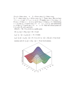
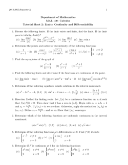

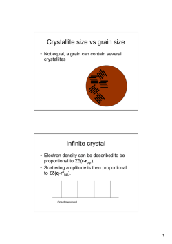
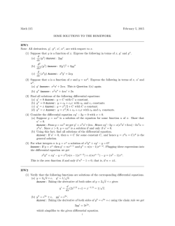
© Copyright 2026