1. Art and Diseño

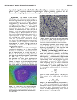
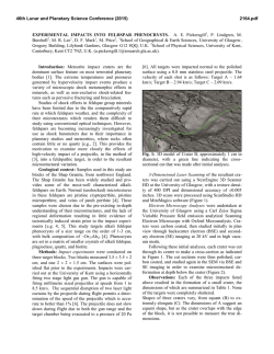
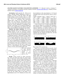
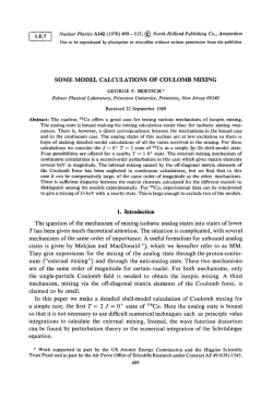
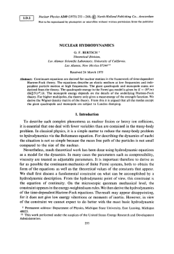
NUCLEAR
PHYSICS A
Nuclear Physics A556 ( 1993 ) 136- 146
Nosh-Holland
Coulomb reacceleration as a clock for nuclear reactions
G.F. Bertsch ’ and CA. Bertulani 2
National Superconducting Cyclotron Laboratory, ~~ich~ga~State University, East Lansing,
MI 48824-1321, USA
Received 9 December
1992
Abstract: A possible measure of the time scale for projectile break-up reactions is the acceleration
in the target Coulomb field following the excitation process. We model this by solving the
time-dependent
Schrodinger equation in one dimension, comparing with simple arguments
based on the uncertainty principle. We find that momentum shifts are generally much larger
than given by simple arguments based on classical mechanics and the uncertainty principle.
1. Introduction
Recently, there has been a rapid development of techniques to study properties of
radioactive nuclei, probing them by their reactions as projectiles on nuclear targets ’ ).
These nuclei are so short-lived that the standard technique of using them as targets to
study their properties is not often possible. Examples of such nuclei are “Li, “Be and
14B.
In particular, we cite the case of *rLi. Much of what we know about this nucleus was
obtained in reactions with secondary beams. It is an unusually large nucleus, which is
due to loosely-bound neutrons orbiting around a ‘Li-core. The weak binding also gives
rise to an enormously enhanced break-up cross section in a Coulomb field.
The motivation of this paper is a recent experiment at the Superconducting Cyclotron of
the Michigan State University 2), measuring the velocities of the fragments in reactions
of “Li projectiles. An intriguing effect was observed, that ‘Li fragments have on the
average a higher velocity than the beam velocity. This was qualitatively explained as an
effect of the Coulomb field of the target. Up to the break-up point, “Li is decelerated
by the Coulomb field. After the break-up, 9Li is accelerated by the same field. Since it is
lighter than “Li ‘Li will be detected with a higher velocity than the incoming projectile.
For the same reason, the neutrons will be observed slower than the projectiles. This was
also observed in the experiment 2 ).
In order for this mechanism to be effective, the break-up must occur close to the target.
One could imagine using the reacceleration as a clock to measure the time it takes for the
’ Present address: Prof. G.F. Bertsch, Department of Physics, FM- 15, University of Washington,
Seattle, WA 98195, USA.
2 On leave of absence from Instituto de Fisica, Universidade Federal do Rio de Janeiro, 2 1945 Rio
de Janeiro, Brazil.
~3~S-94~4~93~$06.00
@ 1993-Elsevier
Science Publishers B.V. All rights reserved
G.F. Bertsch, CA. Bertulani / Coulomb reacceleration
system to break up. For the “Li break-up, the dipole excitation
strength function
137
is rather
narrow, and if the excited state were treated as a resonance, a quite long time would be
required for it to break up*. It seems that the experimentally observed reacceleration is
incompatible with the resonance interpretation.
We therefore thought it would be interesting to analyze the process in a completely
quantum-mechanical
way, using the time-dependent
Schrodinger equation. By varying
conditions of the hamiltonian,
we hope to understand when classical arguments can
be used, treating the steps of deceleration, excitation, reacceleration and break-up as
independent
processes. Of course in principle one must calculate amplitudes at each
step, which can cause differences from the classical picture 3 ).
Before proceeding to our model, we mention that Coulomb reacceleration is an important issue in another context as well. Measuring Coulomb dissociation of a fast projectile
has been proposed to determine the radiative capture cross section of interest for astrophysics 4). Using first-order perturbation theory the coincidence measurements of differential cross sections for a given relative energy of the fragments can be directly related to
the radiative capture cross sections. However, if the fragments are much reaccelerated by
the Coulomb field of the target after the break-up this method does not work. Recently 5 ),
this method has been used to study the reaction Pb (8B, p + 7Be) which hopefully can give
information about the radiative capture cross section for the reaction ‘Be(p, Y)B useful
to the solar neutrino problem. In the Coulomb break-up process ‘6 is excited to a state
in the continuum, decaying by a proton tunnelling through the Coulomb barrier. In this
case it is important to know if the time delay for the tunnelling allows the Coulomb field
of the target to be neglected.
In this paper we address the Coulomb reacceleration problem. Since the problem is
rather complicated in three dimensions we simulate it as a one-dimensional
problem
with characteristics which are of quite general nature. The aim of this work is to assess
the relevance of Coulomb reacceleration and compare the solution of the time-dependent
Schrodinger equation with the predictions of classical theory. If the classical theory were
reliable, the features of Coulomb reacceleration might be easily understood and used in
the planning of future experiments.
2. A Schriidinger model for break-up and reacceleration
We shall discuss the projectile break-up physics in terms of a particle bound to a
potential well which represents the projectile core. The particle is initially bound and is
then excited into the continuum by the interaction with the target. We treat the dynamics
in the frame of the projectile, so the potential well of the projectile is fixed in space. We
consider only the dipole component of the Coulomb interaction with the target, which
produces a linear field acting on the particle. The coordinate frame undergoes acceleration
* The width of the excitation in 11Li is about 0.5 MeV, and beam velocity in this experiment was
about 0.25~. In the resonance interpretation, this implies that the projection travels on the average
a distance vdt = hv/r
100 fm before breaking up.
138
G.F. Bertsch, C.A. Bertulani / Coulomb reacceleration
due to the Coulomb
additional
force on the projectile
linear potential
core, and this gives rise effectively
6). The hamiltonian
ihdlv =
_h2V2
2mv
dt
where V, is the core potential
+
equation
V,V + (z, -
to an
to be solved is then given by
-CIA)r~Ev,
and E is the electric field from the target. For our purposes,
we can assume that the the projectile moves almost undeflected in the target Coulomb
field. In this case the Coulomb field of the target acting on the projectile has two components: (a) one perpendicular
and (b) another parallel to the projectile direction of
motion. The time-dependent
interaction potentials of a unit charge with these fields are
given by
I/i,(f) =
Zre2
uot
(b2
+
v,+2)312
2,
(1)
where b is the impact parameter and vo is the projectile velocity, and we have used the
dipole approximation.
In these equations the time t is measured from the point when the
projectile and target are closest to each other. The longitudinal potential l$ (t) changes
sign during the collision and is much less effective in the Coulomb break-up than the
transverse one.
The above posed problem, solving the three-dimensional
Schrodinger equation in a
time-dependent
external field, is computationally
rather involved for the simple qualitative physics that we want to extract. We therefore made a rather drastic additional
simplification and use the one-dimensional
Schrodinger equation. Physically, this corresponds most closely to the transverse dynamics. The transverse field is most important
for the break-up, and transverse accelerations give rise to the angular deflection of the
fragments from the beam axis.
We solve the time-dependent
Schrodinger equation by a finite difference method, calculating the wave function at time t + At in terms of the wave function at time t, according
to the following algorithm ’ ),
[6(t)
+ VN] u(t).
>
(2)
In this equation, Vc = VL(t) is time-varying Coulomb field, l$ is the nuclear potential
responsible for the binding, r = hAt/4m (Ax)~ and m is the nucleon mass. The seconddifference operator A (2) is defined
Ac2’U,(t)
= uj+l(t)
+ uj_l(t)
-2u,(t),
(3)
with u, (t ) E u (x,, t ) the value of the wave function on the mesh point x,. This method
has the advantages that it is accurate to fourth order in Ax, is explicitly unitary and is
easily programmed.
G.F. Bertsch, CA. Bertulani / Coulomb reacceleration
139
In the “Li break-up, the charges are Z, = 0 and Z,/A = 318. However, for our model
study it is convenient to think about a proton in a nonaccelerated potential, i.e. Z, = 1
and Zt/A = 0, and we shall discuss the momentum distributions for this situation.
The break-up
are calculated
probabilities
for a given impact parameter
and as a function
of time t
from the relation
= 1 - I(W)lm)12
P(b,ll
where us = u (-x)
is the initial bound-state
tum in the state is given by
(P(t))
= @(t)lPju(t))
>
(41
wave function.
= hx(u,
The expectation
+ u,+,)(u,+,
of momen-
- u,)/2iAx.
Physically, we are only interested in the momentum of the unbound particle, so we will
consider also the projected wave function that has the bound-state component removed.
This is defined
UC =
(
N u(+x)
- (u(+x)luo)
>
(6)
uo )
where N normalizes the continuum wave function, uc, to unity. The reason for renormalizing the wave function is the following. If we calculated the total momentum in our wave
function u(t), this would average over the momentum of both parts of the final state,
with the particle bound and in the continuum. The experiment however only measures
the momentum associated with the continuum particle, and its result may be expressed
as the momentum per continuum particle. Thus the calculated number should be the
total momentum divided by the continuum emission probability, which is the same as
the momentum of uc.
In first-order perturbation theory the continuum wave functions have an average momentum zero, (p) = 0, although the root-mean-square
momentum m
is nonvanishing. This can be easily seen in the dipole approximation, as a consequence of the symmetry
of the initial wave function and the dipole excitation operator. In the nonperturbative
treatment, the Coulomb potential acts to all orders, and the continuum wave function
can have nonzero (p).
We want to compare the quantum predictions with simple classical models. Let us
assume that the particle is fixed to the projectile until the projectile reaches the point z
along its trajectory, with z = 0 being the closest approach point. The particle is assumed
to be freely accelerated after that. The total momentum given to the emitted particle is
P(Z)
= q$
(1 -
z+/~)
.
For a free particle, the starting point is z = -~cj and the momentum
Pfree =
p(-x)
= 2ZTe2/bv
transfer is
(71
As a first break-up model, let us assume that the particle gets no momentum until the point
of closest approach. There it goes to a continuum state immediately and is accelerated
140
G.F. Bertsch, C.A. Bertulani / Coulomb reacceleration
0.2_-----------I
'I
-200
-100
0
100
t
I ' L t I I ' L I I L
200
300
400
[fm/cl
Fig. 1. Transition probability for a bound particle in a square-well continuum states due to a perturbing Coulomb potential, as a function of the collision time. The solid(dashed) curve corresponds
to impact parameter b = 15( 50) fm.
by the target Coulomb
above formula,
field for the entire time afterwards.
We thus take z = 0 in the
(8)
Pinstantaneous= Z-re2/bv
The other classical model is the resonance decay model. Here the excited state decays
exponentially with a mean life 7 and the average acceleration is given by
Pres =
dt dP(t)ldt
JI
co $
exp(-(t’
- t)/r)p(vt’).
(9)
3. Numerical results
We first define a one-dimensional
potential VN that simulates the conditions of the
“Li bound state. We take a square-well potential with a depth of 1.43 MeV and a width
of 3.2 fm. This potential supports a single bound state of energy E = -0.2 MeV and
root-mean-square
extension of 7 fm. For the Coulomb excitation, we assume a projectile
velocity of v = kc, corresponding to a laboratory energy Elab _ 30 MeV/nucleon,
and
a target charge corresponding to Pb, ZT = 82. A grid adequate for our purpose has 500
spatial mesh points separated by 0.4 fm and 1000 time mesh points separated by 1 fm/c.
In fig. 1 we show the transition probability calculated from eq. (4) for a collision with
impact parameter b = 15 fm (solid line) and b = 50 fm (dashed line). The transition
occurs over a time interval At N b/u. The result for b = 50 fm is close to the perturbative
Coulomb excitation calculation, but the probability at b = 15 fm approaches unity and
the perturbative calculation is inaccurate. Note that at z = 0 the probability only reaches
i of its asymptotic value, making the extreme instantaneous
model doubtful.
G.F. Bertsch, C.A. Bertulani / Coulomb reacceleration
0.06
141
-
Fig. 2. Particle density distribution for the ground-state (solid line) and continuum states at several
time instants and as function of the position. The impact parameter in this collision is b = 15 fm.
In fig. 2 we plot the particle probability density as a function of position at several
instants of time. The impact parameter here is b = 15 fm. The solid line corresponds
to the ground state, normalized to unity. The dashed lines were obtained by projecting
out the continuum part of the time-dependent
wave function and renormalizing to unit
probability. One observes that as time evolves the particle moves to the right. There
is also a small probability that it moves to the left due to reflection on the borders of
the square-well potential. As the particle moves, its wave packet gets more dispersed in
position, as expected. At t = 600 fm/c the transition probability reaches its asymptotic
value and the wave packet is far from the well. With further time evolution, the particle
would eventually be reflected from the far end of the spatial grid.
We next calculate the asymptotic momentum from eq. (5 ). We expected either the
instantaneous
model or the resonance model to apply. Much to our surprise, neither
describes the results from the time-dependent
SchrGdinger equation. Instead, the momentum transfer is close to the free-particle model. This is shown in fig. 3. Obviously,
coherence effects in the wave function are very important for this observable.
Lest the reader doubt our numerics, we present
order perturbation theory that the excited particle
Consider a particle bound to a harmonic-oscillator
only consider the ground and the first two excited
be V (t ) = x f (t) with f (t ) nonzero only over a
period. Then the second-order wave function is
y = (1 pz2/4mw)
where
I = J”=
dt
IO) - iI~l)(11x10)
an analytic demonstration
in secondcan have the full recoil momentum.
potential. To second order, we need
states. The perturbing potential will
time short compared to the oscillator
- ~r2l2)(2lxll)(llxlo),
f(t).
The expectation of the momentum
operator to first order in I
142
G.F. Bertsch, C.A. Bertulani / Coulomb reacceleration
O’““‘““‘.‘“““““.“..,.’
15
20
25
30
35
40
45
Fig. 3. Momentum of the particle excited to the continuum as a function of impact parameter.
Solid curve is the result from the time-dependent
Schrodinger equation with a potential giving
weak binding. The dashed curve is corresponding momentum imparted to a free particle in the
same time interval. These numbers differ slightly from eq. (7) due to the finite integration time.
is given by
(P) = 2~Z(Ol4l)(ll~lO).
We put in the harmonic-oscillator
matrix elements,
(01x11) = ,,/m
(101
and (01~11) =
-i
irno and find for small t the result (p) = I as expected from classical physics. Let
r
us now project out the excited state. The wave function is
Vc = 11) - ;izl2)(21x/l),
and the expectation
of the momentum
(p)C =
is
~~(ll~l2)~1lW.
(11)
If the matrix elements of p and x were the same as in eq. (9), the expectation of p would
be half the free-particle value, in agreement with the instantaneous
break-up model.
However, the matrix elements are actually larger by factors of a, so the excited state
also has the free-particle momentum. Note that if we did not renormalize the projected
wave function the momentum expectation would be of order of Z3, much smaller than
with renormalization
for small I. This is because, for small I, the particle tends to remain
in its ground state for which (p) = 0. But since the particle reaching the detector is in a
continuum state, a renormalization
is necessary to compare with the experiment.
This shows that the classical intuition fails for weakly-bound particles. However, the
behavior of a particle excited to a true resonance should be closer to the classical. In a
resonance, the particle is held in by a barrier and the momentum it acquires is quickly
exchanged with the potential barrier.
G.F. Bertsch, C.A. Bertulani / Coulomb reacceleration
143
Fig. 4. Square well plus square-barrier potential used to study resonance decay. The potential
parameters are: Vc = -5 MeV, a0 = 8 fm, Vi = 5 MeV and at = 3 fm. The bound-state wave
function is shown by the dashed line. Its binding energy is 3.3 MeV.
To see what happens
in this case we consider
nant state. We chose a form for the potential
with the ground-state
wave function
a potential
with a barrier
using a square-barrier
in fig. 4. The resonance
to make a reso-
form, shown together
is at an energy
of 1.1 MeV
of 0.3-0.4 MeV. These properties may be deduced from the decomposition of the time-dependent
wave function into energy eigenstates or by examining the
decay in time of the resonant state, as shown in figs. 5 and 6. The 0.4 MeV width of
the resonance translates into a mean life-time of 500 fm/c, allowing to the projectile to
travel 100 fm beyond the point of excitation under our conditions for excitation. Clearly
for impact parameters of the order of 15 fm, the reacceleration following break-up will
and has a width
:::i
I
.
l
L
3
0.10
.
.
.
.
0.05
-
.
.
.
.
.
- .
0
Dooo
-$oD o
0.006..,““““‘~“,‘,““““‘,’
0.5
1.0
0.0
E
0
0
1.5
0
2.0
0
.
0
2.5
.’
3.0
[MeV]
Fig. 5. Amplitudes of energy eigenstates in the asymptotic time-dependent
wave function,
lail = i(u, lu(t 1) 1for the excitation at b = 15 fm. The states are discrete because of the finite
size of the spatial domain. The resonance only appears in states with i odd (tilled circles), because
the resonance has odd parity. The amplitudes
with i even are shown with open circles.
144
G.F. Bertsch, C.A. Bertulani / Coulomb reacceleration
t [f&cl
Fig. 6. Formation and decay of the resonant state for a collision with b = 15 fm. Plotted is the square of the overlap of the time dependent wave function with the state xlu,$,
PR = i(u(t)lxluo)l’ /(u~lx21u~). The dashed line shows exponential decay with a time constant
T = 500 fm/c.
be quite small and we expect the momentum of the emitted particle to be nearly zero.
The results of the time-dependent
Schrodinger calculation belie our naive expectations.
Fig. 7 shows the net momentum of particles emitted from the square-barrier potential
together with the free-particle momentum and the prediction of the classical resonance
model. Although there is some reduction as compared to the case with the weak binding potential, the momentum is far larger than in the resonance model. Obviously, the
barrier penetration is strongly connected with the excitation process. In our model, the
resonance is penetrated preferentially on one side where the barrier is lower. The qualitative behaviour of this result is independent of the strength of the exciting field, and
is essentially reproducible in second-order perturbation theory. The net momentum per
emitted particle is linear in the external field in second-order perturbation theory, just as
the classical momentum.
4. ConcIusion
Our results suggest that Coulomb acceleration is intrinsically quantum-mechanical
for
conditions typical in light nuclei. One cannot approximate its effects by assuming that it
only acts in the post-break-up phase of the reaction. The accelerations can be much larger,
and experiments that use Coulomb break-up to measure properties of the nucleus may
be more problematic as a consequence of the more persistent acceleration. For example,
this technique was used to infer the dipole excitation strength for the 6Li --+ 4He + d
break-up in ref. * ).
G.F. Bertsch. CA. Bertulani / Coulomb reacceleration
20
30
b
40
145
50
[fml
Fig. 7. Momentum shift of the continuum particle excited from the square-barrier potential, as a
function of the impact parameter in the collision (solid curve). The dashed curve is the momentum
transfer in the instantaneous emission model, eq. (8) and the dotted curve is the prediction from
classical resonance decay, eq. (9).
In the break-up reaction l1Li -+ 9Li + neutrons, the neutrons were observed in a very
narrow cone about the beam axis 9). In our model, there would be essentially no transverse
momentum transfer associated with the Coulomb trajectory of the Li projectile. This
would help preserve the narrowness of the angular distribution in the laboratory frame,
given a neutron momentum distribution predicted by first-order perturbation theory.
Qualitatively, we did find a suppression of the postacceleration when the particle was
excited to a narrow resonance. This clearly shows that the time delay in emitting the
particle can play an important role, although one that does not seem to be easy to estimate.
However, we must emphasize again that these results were obtained for a greatly oversimplified model, putting all of the physics into one dimension. It would be much more
realistic to study the three-dimensional
Schrodinger equation. Then one can separately
treat the excitation, which occurs dominantly in the transverse direction, and the reacceleration, which is observed in the longitudinal direction. It seems to us to be worthwhile
to pursue this, in view of the potential importance of reacceleration both as a measuring
tool and as an obscuring agent in the application of Coulomb break-up.
This work was supported by the NSF under grant PHY 90-17077 and by the DOE
under grant DE-FG06-90ER4056
1.
146
G.F. Bertsch, CA. Bertulani / Coulomb reacceleration
References
1) Proc. Int. Symp. on the structure and reactions with unstable nuclei, ed. T. Suzuki, Niigata,
Japan (1991)
2) K. Ieki et al., MSU/NSCL preprint ( 1992) to be published
3) R. Shyam, P. Banerjee and G. Baur, Nucl. Phys. A540 (1992) 341;
G. Baur, C.A. Bertulani and D. Kalassa, Nucl. Phys. A550 (1992) 527
4) G. Baur, CA. Bertulani and H. Rebel, Nucl. Phys. A458 (1986) 188
5) M. Gai, private communication
6) G. Bertsch and R. Schaeffer, Nucl. Phys. A277 (1977) 509
7) P. Bonche, S. Koonin and J.W. Negele, Phys. Rev. Cl3 (1976) 1256
8) J. Kiener et al., Phys. Rev. C33 (1991) 2195
9) R. Anne et al., Phys. Lett. B250 ( 1990) 19