1. Art and Diseño

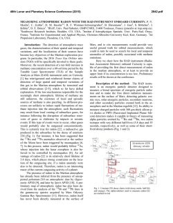
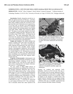
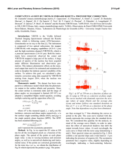
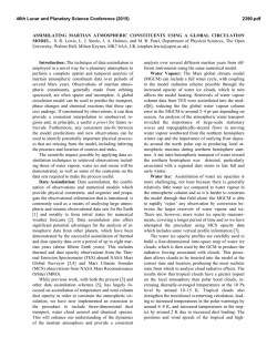
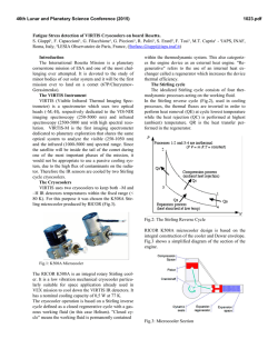
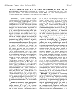
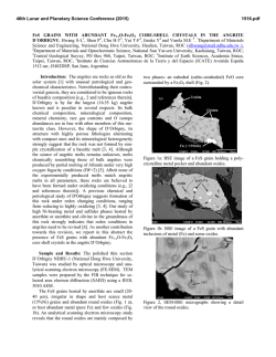
Atmos. Chem. Phys., 15, 1175–1190, 2015
www.atmos-chem-phys.net/15/1175/2015/
doi:10.5194/acp-15-1175-2015
© Author(s) 2015. CC Attribution 3.0 License.
On the use of radon for quantifying the effects of atmospheric
stability on urban emissions
S. D. Chambers, A. G. Williams, J. Crawford, and A. D. Griffiths
Australian Nuclear Science and Technology Organisation, Locked Bag 2001, Kirrawee DC, NSW 2232, Australia
Correspondence to: S. D. Chambers ([email protected])
Received: 1 August 2014 – Published in Atmos. Chem. Phys. Discuss.: 8 October 2014
Revised: 5 December 2014 – Accepted: 19 December 2014 – Published: 2 February 2015
Abstract. Radon is increasingly being used as a tool for
quantifying stability influences on urban pollutant concentrations. Bulk radon gradients are ideal for this purpose, since
the vertical differencing substantially removes contributions
from processes on timescales greater than diurnal and (assuming a constant radon source) gradients are directly related to the intensity of nocturnal mixing. More commonly,
however, radon measurements are available only at a single height. In this study we argue that single-height radon
observations should not be used quantitatively as an indicator of atmospheric stability without prior conditioning of the
time series to remove contributions from larger-scale “nonlocal” processes. We outline a simple technique to obtain an
approximation of the diurnal radon gradient signal from a
single-height measurement time series, and use it to derive a
four category classification scheme for atmospheric stability
on a “whole night” basis. A selection of climatological and
pollution observations in the Sydney region are then subdivided according to the radon-based scheme on an annual and
seasonal basis. We compare the radon-based scheme against
a commonly used Pasquill–Gifford (P–G) type stability classification and reveal that the most stable category in the P–G
scheme is less selective of the strongly stable nights than the
radon-based scheme; this lead to significant underestimation
of pollutant concentrations on the most stable nights by the
P–G scheme. Lastly, we applied the radon-based classification scheme to mixing height estimates calculated from the
diurnal radon accumulation time series, which provided insight to the range of nocturnal mixing depths expected at the
site for each of the stability classes.
1
Introduction
The concentrations of gaseous and particulate pollutants in
the atmosphere are governed by the rate at which they are
emitted from their respective sources, lost by various sink
mechanisms (including surface deposition and in situ chemical transformations), and characteristics of the atmospheric
volume into which they mix (e.g. Veleva et al., 2010; Perrino
et al., 2001, 2008; Avino et al., 2003; Duenas et al., 1996).
This “mixing volume” (or mixing depth) changes diurnally
over land, typically reaching maximum values early in the
afternoon, and minimum values immediately prior to sunrise. In the simplest of cases (cloud-free), daytime mixing
depth is determined primarily by the combined strength of
convective turbulence (thermal circulations driven by solar
heating of the Earth’s surface) and mechanical mixing (related to wind speed and surface roughness). Nocturnal mixing depth, on the other hand, results from a balance between
mechanical mixing and its suppression by thermal stratification in the lower atmosphere (e.g. Collaud Coen et al., 2014;
Williams et al., 2013; Stull, 1988).
During winter in Sydney, as for many urban centres, accumulated domestic heating emissions combine with exhaust from peak-hour traffic in the shallow morning inversion
layer, resulting in “brown haze” and pollutant levels that can
exceed threshold guidelines (e.g. Hinkley et al., 2008; Gupta
et al., 2007; Corbyn, 2005; Duc et al., 2000; Leighton and
Spark, 1997; Liu et al., 1996). In summer, however, photochemical pollution events are more common; their severity
linked to prevailing winds and cloudiness (Hart et al., 2006;
Leslie and Speer, 2004; Azzi and Johnson, 1994; Hawke and
Iverach, 1974). Clearer understanding of the processes that
lead to haze or smog exceedance events, as well as an ability
to quantify their magnitude, is important for assessing po-
Published by Copernicus Publications on behalf of the European Geosciences Union.
1176
tential health impacts on residents, as well as identifying the
need for, and evaluating the efficacy of, emissions mitigation
strategies.
The term “atmospheric stability” – sometimes used synonymously with mixing depth – has been closely linked to
pollution exceedance episodes in many urban centres (e.g.
Grange et al., 2013; Ji et al., 2012; Perrino et al., 2008;
Desideri et al., 2006; Avino et al., 2003; Duenas et al.,
1996). Numerous measures of atmospheric stability have
been devised and applied with varying degrees of efficacy.
The most accurate of these measures are based on the values of, or ratios between, the near-surface temperature and
wind speed gradients or their turbulent flux counterparts
(Richardson number, Obukhov length, Turbulence kinetic
energy etc.; Foken, 2006; Mahrt, 1999; Leach and Chandler, 1992). However, since these approaches are complex,
expensive and labour intensive, they are also the least common, and often restricted to the duration of specific research
campaigns. More widely used measures such as the Pasquill–
Gifford radiation and turbulence based stability classification
schemes (Pasquill, 1961; Turner, 1964; Pasquill and Smith,
1983; Venkatram, 1996; USEPA, 2007), designed to be determined from routinely available climatological observations, are understandably less representative and versatile.
Furthermore, the interpretation of micrometeorological or
climatological observations necessary for all of these techniques is obfuscated by variability due to the effects of a variety of mesoscale motions operating in the nocturnal boundary layer, including local drainage flows, nocturnal jets, and
intermittent turbulence (e.g. see review in Williams et al.,
2013).
Recently, a growing number of investigators have begun
exploiting the virtues of Radon-222 (radon) as a comparatively simple and economical means of quantitatively gauging atmospheric stability or mixing depth (Wang et al., 2013;
Zhang et al., 2012; Xia et al., 2011; Perrino et al., 2001,
2008; Desideri et al., 2006; Galmarini, 2006; Acker et al.,
2006; Sesana et al., 2003 and references therein; Duenas
et al., 1996; Febo et al., 1996; Porstendörfer et al., 1991;
Fujinami and Esaka, 1987). Radon is an unreactive, poorly
soluble, radioactive gas (t0.5 = 3.82d) that is emitted naturally from ice-free, unsaturated terrestrial surfaces at a rate
that varies slowly both geographically and temporally (0.72–
1.2 atoms cm−2 s−1 ; Turekian et al., 1977; Lambert et al.,
1982; Jacob et al., 1997) and is two orders of magnitude
greater than from open bodies of water (Wilkening and
Clements, 1975; Schery and Huang, 2004). The half-life of
radon is sufficiently long that it can be assumed to be an approximately conservative tracer over the course of a single
night, while being short enough that it does not accumulate in the atmosphere and typically exhibiting an order of
magnitude gradient between the atmospheric boundary layer
(ABL) and the lower troposphere. This combination of physical characteristics makes radon a quantitative proxy for the
effects (outcomes) of near-surface vertical mixing on scalar
Atmos. Chem. Phys., 15, 1175–1190, 2015
S. D. Chambers et al.: Radon-based stability analysis
quantities, and one that is independent of micrometeorological or climatological observations.
It has been demonstrated that near-surface two-point vertical radon concentration gradients constitute an unambiguous measure of vertical mixing and atmospheric stability
(Williams et al., 2013; Chambers et al., 2011; Porstendörfer
et al., 1991; Gogolak and Beck, 1980; Malakhov et al., 1966;
Jacobi and Andre, 1963). The act of vertical differencing efficiently removes most contributions to the observed radon
signal that are related to processes on timescales greater than
the diurnal cycle, including synoptic to seasonal variations in
fetch regions and tropospheric exchanges with the boundary
layer. To date, however, most investigators employing radon
as a proxy for atmospheric stability have had access to observations at only a single height (e.g. Wang et al., 2013; Zhang
et al., 2012; Perrino et al., 2001, 2008; Sesana et al., 2003;
Duenas et al., 1996). If only a single height is available, the
unwanted effects of these larger-scale processes need to be
eliminated by careful conditioning of the radon time series.
The aims of this study are: (i) to demonstrate that radon
observations at a single height can only be used quantitatively as an atmospheric stability indicator if contributions on timescales greater than the diurnal are first removed or reduced by careful conditioning of the time series; (ii) to propose a simple, approximate method for separating these components in a time series of radon observations made from a single height that is well below the
minimum depth of a typical stable nocturnal boundary layer
(≤ 20 m above ground level, a.g.l.); (iii) outline a simple
method for generating a radon-based stability classification
scheme on a “whole night” basis; (iv) demonstrate the effectiveness of this scheme by quantifying the influence of
increasing atmospheric stability on diurnal concentrations
of selected climatological parameters and urban pollutants,
and nocturnal mixing depths; and (v) compare the performance of the radon-based scheme against a more traditional
(Pasquill–Gifford) categorical stability classification scheme
using standard meteorological parameters as input.
2
Site and observations
All observations for this study were made on the grounds
of the University of Western Sydney, Richmond Campus
(33.618◦ S, 150.748◦ E). Richmond is approximately 55 km
inland from the New South Wales coast, 51 km northwest of
the Sydney CBD, and approximately 24 m a.s.l. While the topography in the immediate vicinity of the site is relatively
flat, it is near the western extent of the Sydney Basin, such
that the foothills of the Great Dividing Range lie about 5 km
to the west. Unless otherwise specified, results are derived
from the 5-year period 2007–2011, all times are local Eastern
Standard Time (EST = UTC + 10 h), and the southern hemisphere seasonal definition is employed.
www.atmos-chem-phys.net/15/1175/2015/
S. D. Chambers et al.: Radon-based stability analysis
Continuous, direct, hourly atmospheric radon concentration measurements were made using a 1500 L dual flow loop,
two-filter radon detector (e.g. Whittlestone and Zahorowski,
1998; Chambers et al., 2014). Raw counts and detector operational parameters were logged at half-hourly intervals to
a CR800 logger (Campbell Scientific, Inc.) and integrated to
hourly values for post processing. Air was sampled from a
height of 2 m a.g.l. through 50 mm I.D. PVC pipe at a flow
rate of ∼ 50 L min−1 . A 400 L delay volume was incorporated in the intake line to ensure that thoron (Rn-220) concentrations entering the detector were less than 0.5 % of their
ambient values. The detector had a response time (time to
half-peak magnitude) of 45 min, and a lower limit of determination (defined here as the equivalent radon concentration for a detector counting error of 30 %) of 30 mBq m−3 .
The detector’s instrumental background increases approximately linearly with time, primarily as a function of the accumulation of the long-lived particulate radon daughter Pb210 on the second filter. Background checks were performed
every three months and the linear (R 2 = 0.99) background
model removed from the raw hourly counts before calibrating to final concentrations. Detector calibrations were also
performed every 3 months, by injecting radon for 5 h from a
flow-through Pylon 245 kBq ± 4 % Ra-226 source (traceable
to NIST standards) at a rate of 80 cc min−1 . The coefficient
of variability of calibration coefficients over the study period
was 5.2 %. The combined error on an hourly concentration
estimate of 100 mBq m−3 is expected to be 17 %. This measurement uncertainty reduces with longer averaging times as
∼ N −1/2 for N hourly samples. Furthermore, the contribution to this uncertainty by the detector’s counting error decreases with increasing radon concentration (e.g. from 30 %
at 0.03 Bq m−3 to 3.5 % at 1 Bq m−3 ).
Hourly observations of climatological parameters (wind
speed, direction, air temperature and humidity), as well as
standard air quality parameters (NO, NO2 , Ozone, SO2 ,
PM2.5 ), were provided by the New South Wales Office of
Environment and Heritage from a site adjacent to the radon
observations. Wind speed and direction were recorded at
10 m a.g.l., other climate sensors and the intake for air quality observations was situated at ∼ 5 m a.g.l., on the roof of a
small enclosure.
It should be noted that slight calibration problems were
evident with the externally provided NO and SO2 concentrations. An approximately linear drift in the NO data of
0.54 ppb per year was identified and removed, but some uncertainty remains in the absolute values. A slight negative
drift in the SO2 calibration was also evident, but the coarse
resolution of the data at low concentrations made it difficult
to correct. Consequently, small negative SO2 values are occasionally reported for periods of low concentration. However,
since the relative changes in concentration are the focus of
this study, these issues with the absolute calibrations will be
overlooked.
www.atmos-chem-phys.net/15/1175/2015/
1177
3
Development of a radon-based stability index
The observed variability of long-term atmospheric radon
measurements represents the superposition of influences acting on a range of scales, including: synoptic to seasonal
changes in air mass fetch; synoptic-scale tropospheric exchanges with the boundary layer (via fronts and deep convection); geographically generated mesoscale circulations;
and diurnal vertical mixing within the boundary layer. Assuming that local diurnal contributions to the observed radon
signal can be meaningfully disentangled from the largerscale (“non-local”) contributions, and neglecting the decay
of radon over a single night, the nocturnal accumulation of
radon near the surface should be primarily controlled by two
factors: (a) the mean radon flux from a representative local
fetch region, and (b) the strength and extent of vertical mixing, which is closely related to stability and the depth of the
nocturnal boundary layer.
3.1
The seasonal cycle of radon at Richmond
The composite seasonal cycle of radon at Richmond (Fig. 1a)
is characterised by low concentrations November through
February and higher concentrations March through October
(see also Crawford et al., 2013). Ignoring May for a moment,
at least ∼ 30 % of the 4.2 Bq m−3 amplitude of mean monthly
radon concentrations seen in Fig. 1a is attributable to “nonlocal” effects. This can be seen by inspection of the mean
afternoon (∼ 15:00 EST) radon concentrations in the composite diurnal cycles presented in Fig. 1c (see also Fig. 4a),
which exhibit a seasonal range of about 1.5 Bq m−3 . Afternoon radon values near the surface tend to be representative
of the mean concentration through the depth of the daytime
convective boundary layer (CBL), which is typically 1 km or
more and changes only slowly from day to day in response to
the passage of synoptic scale weather systems. Seasonal migration of the subtropical ridge leads to variations in the recent terrestrial source regions for radon, and frontal systems,
deep convection and variations in the depth of the capping
inversion affects the degree of dilution of radon within the
CBL.
Climatological summaries of the Sydney Basin region
(e.g. Crawford et al., 2013; Chambers et al., 2011) show
that regional flow for this region in summer is predominantly
easterly to southerly, with recent land fetch typically less
than half a day. In winter, however, regional flow is often
south westerly to westerly, with recent terrestrial fetch over
south eastern Australia of the order of 2–3 days. In May,
low mean wind speeds often result in longer air mass timeover-land, leading to particularly large nocturnal radon levels
(Fig. 1a, b).
The remaining ∼ 70 % of the seasonal variation observed
in mean surface radon concentrations at Richmond is attributable to local diurnal effects. The composite diurnal cycle of radon at Richmond (Fig. 1c) is characterised by peak
Atmos. Chem. Phys., 15, 1175–1190, 2015
1178
S. D. Chambers et al.: Radon-based stability analysis
30
15
10
5
0
(c)
4
3
2
1
F M A M
J
J
A
S O N D
12
9
6
3
0
J
Summer
Autumn
Winter
Spring
15
Radon (Bq m-3)
20
(b)
Wind speed (m s-1)
Median
10th perc.
90th perc.
25
Radon (Bq m-3)
18
5
(a)
0
J
F M A M
Month of composite year
J
J
A
S O N D
0
3
6
9
12
15
18
21
Hour of composite day
Figure 1. (a, b) Monthly distributions (10th, 50th and 90th percentiles) of radon and wind speed, (c) hourly mean diurnal composite radon
by season, at Richmond.
concentrations near sunrise, when the nocturnal boundary
layer is at its shallowest, wind speeds tend to be at their
lowest and the influence of local sources dominate. Minimum values are found in the mid-afternoon, when the convective boundary layer is at its deepest (maximum dilution),
and radon source influences are dominated by the air mass
fetch history of the last ∼ 2 weeks (see discussion above).
The timing of the diurnal cycle (Fig. 1c) changes according to seasonal variations in the intensity and duration of incident radiation, with morning peak concentrations shifting
from 05:00 EST in summer to 07:00 EST in winter, and the
duration of the afternoon minimum period contracting from
6 h in summer to 2 h in winter. Typically lower mean wind
speeds (Fig. 1b) and colder drier conditions in autumn and
winter generate weaker mixing, leading to shallower nocturnal inversions with high radon levels.
3.2
Isolating the stability-related signal
Atmospheric stability indices are designed to provide measures of the atmosphere’s capacity to support vertical mixing by local turbulence processes. Variations in the observed
radon signal due to the “non-local” processes described
above, however, are not directly related to atmospheric stability and can be comparable in magnitude to the stabilityrelated variations. The “non-local” radon signal is largest for
sites situated near the coast, due to the strong land/ocean contrast in the radon source function, but will be evident to some
degree at all sites since the 3.8 day half-life of radon means
that fetch regions over the last two weeks or more influence
the observed signal. It is therefore important to characterise
and remove (or neutralise) the effects of these “non-local”
variations prior to application of radon as a quantitative indicator of atmospheric stability.
When vertically resolved radon measurements are available from towers, a two-point radon gradient can be calculated between the lowest and highest intake levels for the
purpose of characterising bulk mixing characteristics in the
Atmos. Chem. Phys., 15, 1175–1190, 2015
nocturnal boundary layer (Chambers et al., 2011; Williams et
al., 2013). This vertical differencing effectively removes contributions to the absolute radon signal on timescales greater
than the diurnal. To demonstrate this point, 10 days of radon
gradients between 2 and 50 m from another site within the
Sydney Basin (Lucas Heights, 50 km SSE of Richmond) are
presented in Fig. 2. Described in Chambers et al. (2011) and
Williams et al. (2013), this site is located on a broad ridge
18 km from the coast. Topography in the immediate vicinity
is moderately complex, with changes in elevation of ∼ 150 m
within a 1 km radius. 4-day back trajectories (Fig. 3) using
the HYSPLIT model (Draxler and Hess, 1998) indicated that
the increase in daily minimum (afternoon) radon concentrations from day 253 to day 255 in Fig. 2a was a result of
an increasing land fetch over eastern Australia. On day 257,
both detectors indicated an abrupt reduction in radon concentration corresponding to a synoptic change in air mass
fetch from terrestrial (south westerly) to oceanic (south easterly). Inspection of the corresponding radon gradient time series (Fig. 2b), however, shows no significant influence from
either the slow or the abrupt fetch changes. Instead, the
maximum radon gradient values attained each night are primarily a measure of the amount of locally sourced radon
trapped within the nocturnal inversion. Assuming a local
radon source function that is approximately constant in time
and space, the gradient time series is thus predominantly a
function of stability.
Unfortunately, few sites are set up to conduct vertical
radon gradient observations. However, the particular qualities of radon, together with an understanding of its distribution in the boundary layer, allow us below to construct an approximate vertical radon gradient using only measurements
at a single height near the surface, for use as a stability indictor.
In the mid-afternoon (Fig. 1c), the ABL is relatively
well-mixed from the surface to the synoptic inversion and
radon measurements close to the surface are representative of
www.atmos-chem-phys.net/15/1175/2015/
S. D. Chambers et al.: Radon-based stability analysis
1179
(a)
2 m radon
50 m radon
6
Radon (Bq m-3)
4
2
0
(b)
Gradient (2-50m)
2
1
0
250
252
254
256
258
260
Day of 2009
Figure 2. (a) 2 and 50 m a.g.l. hourly radon concentrations at Lucas Heights, 30 km southwest of Sydney, in September 2009, and (b) the
corresponding hourly radon gradient.
bulk ABL radon concentrations (e.g. Chambers et al., 2011;
Williams et al., 2011; Moses et al., 1960). When the ABL
is deep and well-mixed, radon concentrations reflect the collective influence of all sources (decay weighted) over the air
mass’s recent (∼ 2-week) fetch history. After sunset, however, in the absence of low cloud or high winds, an inversion
layer begins to form from the ground up as a result of the
growing thermal stratification (the stable nocturnal boundary layer, SNBL) (e.g. Collaud Coen et al., 2014; Sesana et
al., 2006; Stull, 1980). The radon concentration in the residual layer (RL), the air residing between the top of the SNBL
and the previous day’s synoptic inversion, remains similar to
that of the previous day’s ABL (ignoring radon decay; e.g.
Kondo et al., 2014) and can therefore be approximated from
the previous afternoon’s minimum (well-mixed) radon concentration near the surface. By linearly interpolating minimum radon concentrations from one afternoon to the next, it
is therefore possible to produce a radon time series similar
to that which might be measured by a radon detector with
an intake height within the RL. Below the nocturnal inversion, however, the radon concentration of the SNBL evolves
largely independently of the overlying radon concentration.
Since wind speeds are typically < 1 m s−1 on stable nights,
the radon that accumulates between the surface and the capping inversion of the SNBL (e.g. morning peak of Fig. 1c)
is derived primarily from local sources (i.e. within less than
a 40 km radius; Chambers et al., 2011). A radon “pseudogradient” can thus be formed by computing the difference between the near-surface observations and the constructed time
series approximating the radon concentrations in the RL.
This pseudo-gradient will be substantially free from variability associated with “non-local” processes and thus mainly in-
www.atmos-chem-phys.net/15/1175/2015/
Figure 3. One week of 4-day HYSPLIT back-trajectories depicting
conditions of high (red), moderate (green) and low (blue) terrestrial influence on air masses arriving at Lucas Heights, NSW. Each
trajectory is the average of five hourly trajectories between 13:00–
17:00 LST each day.
fluenced by the strength of the local radon source function
(approximately constant) and atmospheric stability.
3.3
Features of the radon pseudo-gradient
As an example of the above technique, a 5-week subsection
of the 5-year Richmond radon time series is presented in
Fig. 4a. Periods of oceanic fetch are evident where daily minimum concentrations drop below 0.5 Bq m−3 , as well as periAtmos. Chem. Phys., 15, 1175–1190, 2015
1180
S. D. Chambers et al.: Radon-based stability analysis
Radon (Bq m-3)
20
2 m radon
Interpolated
(a)
10
0
18
Pseudo-gradient
(b)
12
6
0
240
245
250
255
260
265
270
Day of 2007
Figure 4. (a) Hourly radon observations at Richmond in September 2007, and afternoon interpolated values, and (b) the Richmond radon
gradient (difference between observed and interpolated radon concentrations).
ods of multi-day terrestrial fetch with daily minimum radon
concentrations of 3–4 Bq m−3 . Included in this figure is a
linear interpolation between afternoon minimum radon concentrations (red line). The routine used to generate this line
identified the minimum hourly radon concentrations between
12:00–18:00 EST each day and linearly interpolated between
them. On occasion, when there was a large change in fetch
(terrestrial to oceanic) or a large nocturnal mixing event, the
difference between the observed radon and the interpolated
values (the “pseudo-gradient”) sometimes went negative. On
such occasions, the routine adjusted the interpolated series
by adding additional linear segments (as few as possible) to
maintain a non-negative “gradient”. A subsection of the resultant pseudo-gradient time series is shown in Fig. 4b.
A feeling for the relative contributions of the “non-local”
and stability-driven contributions to the seasonal cycle of
radon at Richmond can be obtained by separately considering their monthly mean values (Fig. 5a). There is a pronounced seasonality in both components. In the case of the
“non-local” signal, this is mainly due to changes in air mass
fetch, as already discussed. Stability-driven contributions are
smallest in November through February, when wind speeds
are higher (Fig. 1b) and air masses tend to be more humid (fetch predominantly oceanic) so that nocturnal cloud
cover is more common. These factors reduce the strength of
the nocturnal thermal stratification near the surface, leading
to deeper nocturnal boundary layers and lower near-surface
radon concentrations. In March through October, the predominantly terrestrial fetch results in drier conditions and
more cloud-free nights. This enables strong thermal inversions to form near the surface when wind speeds drop, resulting in near-surface radon concentrations that sometimes
exceed 40 Bq m−3 . May exhibits the largest monthly mean
Atmos. Chem. Phys., 15, 1175–1190, 2015
pseudo-gradient, corresponding to the smallest wind speeds
(Fig. 1b).
3.4
Whole-night radon-based stability classification
A mean hourly diurnal composite plot of the radon gradient is presented in Fig. 5b, with the time axis chosen to emphasise the nocturnal radon build-up, which begins around
sunset (18:00) and starts to erode after sunrise (06:00). We
define a 12 h “nocturnal stability window” from 20:00–08:00
(Fig. 5b), chosen to capture the full range of radon concentrations on the majority of nights. The mean radon pseudogradient within the nocturnal stability window was calculated
for each night, and then quartile ranges of the cumulative frequency histogram of this quantity (Fig. 6) were used to define
the following four radon-based whole-night stability classes:
Quartile
Nocturnal mean
radon gradient
Stability
category
Vertical
mixing
Q1
Q2
Q3
Q4
< 2.5 Bq m−3
2.5–6.3 Bq m−3
6.3–11.2 Bq m−3
> 11.2 Bq m−3
Near neutral
Weakly stable
Moderately stable
Stable
Strong
Moderate
Weak
Very weak
While the nocturnal mean radon gradients reported above
are specific to the Richmond site, updated values for any
measurement site can be determined by preparing a cumulative frequency diagram (Fig. 6) for the site in question, and
reading the new quartile ranges off the graph.
After sorting each whole night of the 5-year data set according to this stability classification, we calculated corresponding diurnal composite radon gradient plots (Fig. 7). For
www.atmos-chem-phys.net/15/1175/2015/
S. D. Chambers et al.: Radon-based stability analysis
1181
Figure 5. (a) Monthly means of the interpolated (“non-local”) and pseudo-gradient (diurnal) radon time series, and (b) diurnal composite
plot of the gradient data.
30
75th percentile
Q3
1000
50th percentile
Q2
500
25th percentile
Q1
0
0
5
10
15
20
25
30
Nearly neutral
Weakly stable
Moderately stable
Stable
25
Q4
1500
Radon gradient (Bq m-3)
Cumulative frequency
2000
35
20
15
10
5
Radon bin (Bq m-3)
0
Figure 6. Cumulative frequency histogram of the daily mean
pseudo-gradient in the 20:00–08:00 EST window.
nights classified as near-neutral (Q1), there was little nocturnal accumulation of radon and the amplitude of the diurnal
cycle was 1.5 Bq m−3 . By contrast, nights classified as stable (Q4) showed a rapid radon build-up after sunset, peaking
near sunrise, with a mean diurnal amplitude of 22.9 Bq m−3 .
4
4.1
Results
Evaluation against meteorological data
Standard climatological observations were available at Richmond during the period of this study. Of these observations,
the parameters most easily relatable to measures of stability
and/or mixing are: wind speed, standard deviation of wind
direction, and temperature. Diurnal composite plots of these
parameters, grouped solely by our radon-based stability classification scheme for whole nights, are shown in Fig. 8.
Nocturnal (20:00–06:00) wind speeds were highest for
the nights classified as “near neutral” (on average almost
2 m s−1 ). High wind speeds result in a deep, mechanically
mixed nocturnal boundary layer, and these periods also exwww.atmos-chem-phys.net/15/1175/2015/
16
18
20
22
0
2
4
6
8
10
12
14
Hour of composite day
Figure 7. Hourly mean diurnal composite radon gradient plots for
the four designated nocturnal stability categories. Each curve represents an average of between 410–420 whole days of observations;
whiskers represent ± 1σ .
hibited the smallest diurnal amplitude in wind speed and
temperature as well as a comparatively small standard deviation of wind direction. Such characteristics are consistent
with overcast conditions and the passage of frontal weather
systems. The smallest mean nocturnal wind speeds were observed on nights classified as “stable” by the radon method,
usually dropping below 0.5 m s−1 . However, even the weakly
stable evenings had wind speeds < 1 m s−1 , which is consistent with Sesana et al. (2003) who reported no significant
nocturnal accumulation for wind speeds above 1.5 m s−1 .
The stable nights also exhibited the greatest standard deviation of wind direction, consistent with the presence of meandering mesoscale flows within the shallow SNBL. The amplitude of the diurnal temperature signal in cases identified
as stable was greater than for the other categories, as would
be expected for predominantly clear-sky conditions. Furthermore, atmospheric pressure (not shown) was 2 hPa greater on
Atmos. Chem. Phys., 15, 1175–1190, 2015
1182
S. D. Chambers et al.: Radon-based stability analysis
Figure 8. Mean hourly diurnal composite plots of (a) 10 m wind speed, (b) 10 m standard deviation of wind direction, and (c) 5 m air
temperature.
average in the “stable” cases, consistent with anti-cyclonic
activity and regional subsidence.
4.2
Evaluation against urban pollution data
In the previous section, it was seen that the radon-based atmospheric stability classification scheme is clearly an effective quantitative tool for delineation between various nocturnal atmospheric mixing states. As a further evaluation, we
used the new classification scheme to quantify changes in
various urban pollutant concentrations as a function of atmospheric stability. As can be seen in Fig. 9, despite the “whole
night” resolution of the radon-based stability classification
scheme, it is capable of characterising the influence of nocturnal mixing on primary and secondary gaseous and aerosol
pollutants.
In the case of NO, NO2 and PM2.5 , the most stable atmospheric conditions (shallow mixing depths) identified by
this scheme are associated with dramatically increased nearsurface pollutant concentrations. On average, the diurnal
range of NO increases from 1.6 ppb under well mixed conditions to 14 ppb under the most stable conditions. The corresponding diurnal range increase for NO2 is 2.8 to 9.4 ppb,
and for PM2.5 3.6 to 12 µg m−3 . However, increasing atmospheric stability has the opposite effect on near-surface concentrations of ozone and SO2 . Since ozone is highly reactive, when trapped in a shallow inversion layer (stable class)
surface deposition processes and titration by NO emitted by
vehicles rapidly reduce the concentration. Conversely, when
near-surface wind speeds are higher (near-neutral class),
ozone is mixed downward from the overlying air mass, resulting in higher nocturnal concentrations. Similarly for SO2 ,
when trapped in a shallow inversion layer chemical sink processes rapidly reduce the near-surface concentration of SO2
formerly present in the ABL. Since there are no significant
Atmos. Chem. Phys., 15, 1175–1190, 2015
sources of SO2 in the immediate vicinity of Richmond, no
accumulation is observed leading up to sunrise.
As was the case for the climatological variables, the diurnal behaviour of each pollutant species in each of the radonbased stability categories was clearly consistent with current
knowledge for urban areas (e.g. O3 , Avino et al., 2003; Acker
et al., 2006; Di Carlo et al., 2007; Zhang et al., 2012, Pitari
et al., 2014; SO2 , Jenner et al., 2012; PM2.5 , Gupta et al.,
2007).
While Fig. 9 clearly demonstrates a close correspondence
between mean nocturnal radon accumulation near the surface
and pollutant concentrations, the pronounced differences in
diurnal cycle characteristics between radon (Fig. 7) and urban pollutants (Fig. 9), largely brought about by spatiotemporal differences in their sources and sinks, can result in
low, or highly variable, correlations between radon and specific pollutant concentrations.
4.3
Comparison with Pasquill–Gifford stability
classification
Pasquill–Gifford (P–G) atmospheric stability typing
(Pasquill, 1961; Turner, 1964; Pasquill and Smith, 1983)
is usually employed to facilitate estimates of lateral and
vertical dispersion parameters in Gaussian plume models.
The P–G stability categories employed here were defined
according to the turbulence-based variation of Turner’s
method (Turner, 1964), based on scalar mean wind speed
and the standard deviation of wind direction. In all, there
are seven P–G stability categories ranging from A through
G (Table 1), although for many regulatory applications (and
the turbulence-based version of Turner’s method) the more
strongly stable categories F and G are grouped together.
The key used for assigning the P–G turbulence stability
categories are provided in Tables 2 and 3 (see also USEPA,
2007).
www.atmos-chem-phys.net/15/1175/2015/
S. D. Chambers et al.: Radon-based stability analysis
1183
Figure 9. Mean hourly diurnal composites of (a) NO, (b) NO2 , (c) Ozone, (d) SO2 , and (e) PM2.5 , for each of the four radon-derived
atmospheric stability classifications.
Table 1. Pasquill–Gifford stability class names.
Class
Description
A
B
C
D
E
F
G
Extremely unstable
Moderately unstable
Weakly unstable
Neutral
Weakly stable
Moderately stable
Strongly stable
All hourly data of the 5-year data set was assigned a P–
G turbulence stability category according to Tables 2 and 3.
To best match the classification performed by the radonbased technique, we then assigned “whole-night” P–G stability classes based on the modal (most common) hourly stability category defined over the 9-hour period 21:00–05:00 EST;
a reduced nocturnal window compared to the radon method
was used here to avoid the lag known to exist between hourly
P–G stability categories and radon-separate concentrations
(Duenas et al., 1996). Lastly, we categorised the climatologiwww.atmos-chem-phys.net/15/1175/2015/
Table 2. Lateral turbulence criteria; step 1 of P–G turbulence stability classification.
Initial estimate of
P–G category
A
B
C
D
E
F
Standard deviation of
wind direction σ θ (◦ )
22.5 ≤ σ θ
17.5 ≤ σ θ < 22.5
12.5 ≤ σ θ < 17.5
7.5 ≤ σ θ < 12.5
3.8 ≤ σ θ < 7.5
σ θ < 3.8
cal and pollutant concentration data on a whole-day basis according to the assigned P–G stability class; selected results
are shown in Fig. 10.
Using the radon “gradient” data as a benchmark (Fig. 10a
cf. Fig. 7), the P–G stability classes D-F appear to fall
roughly between the four radon-defined stability classes.
For example, peak radon concentrations for the moderately
and strongly stable classifications in the radon-based scheme
were 13 and 23 Bq m−3 , respectively, whereas the peak “very
Atmos. Chem. Phys., 15, 1175–1190, 2015
1184
S. D. Chambers et al.: Radon-based stability analysis
Figure 10. Mean hourly diurnal composite plots of selected climatological and pollution quantities for whole days categorised by their
dominant nocturnal Pasquill–Gifford stability category: D – neutral; E – weakly stable; F – moderately stable.
stable” P–G turbulence value was 16 Bq m−3 . This indicates
that the P–G “very stable” category is less selective of the
strongly stable nights than the equivalent category in the
radon-based scheme, a fact that is confirmed by a smaller amplitude in the diurnal temperature composite in Fig. 10c (cf.
Fig. 8c). Comparing the morning evolution of near-surface
temperature between days classified as stable by the two
schemes, fewer of the days classified as stable by the P–
G turbulence scheme appear to develop into clear-sky convective conditions than is the case for the radon scheme. In
fact, mornings of P–G “stable” days are cooler than the P–
G “moderately stable” days. Both schemes predict nocturnal
wind speeds of around 0.5 m s−1 under the most stable conditions, whereas the P–G scheme attributes a smaller proportion of wind speed events to the neutral category, as evident
from the higher mean wind speed and greater variability over
the diurnal cycle.
Perhaps most significantly, the fact that the P–G “stable”
category is less selective of the strongly stable nights than
the radon-based scheme means that the relationship between
atmospheric stability and peak nocturnal pollutant concentrations are underestimated by the P–G scheme (Fig. 10e cf.
Atmos. Chem. Phys., 15, 1175–1190, 2015
Fig. 9d for SO2 ; Fig. 10f, cf. Fig. 9e for PM2.5 ). Such discrepancies (30–50 %) can have significant implications for
public exposure records and would influence air quality management.
5
5.1
Discussion
Applicability, limitations and caveats
While the method described here to derive the radon-based
stability classification scheme is applicable to most nearsurface radon (or radon progeny) time series, the absolute
threshold values adopted for the four stability classifications
(shown in Fig. 6) will vary according to site-specific changes
in the frequency distribution of the nocturnal mean radon gradient (see Sect. 3.4). At sites that experience consistent snow
cover or freezing soils, separate stability classifications may
needed for the “warm” and “cold” parts of the year to account for changes to the local radon source function. Similarly, at sites where there is a large summer/winter change
in daylight hours, separate seasonal stability classification
www.atmos-chem-phys.net/15/1175/2015/
S. D. Chambers et al.: Radon-based stability analysis
Table 3. Wind speed adjustments to determine final estimate of P–G
turbulence categories.
Time of day
Initial estimate of
P–G category
10 m wind speed
(m s−1 )
Final estimate of
P–G category
Day
A
A
A
A
B
B
B
C
C
D, E or F
u<3
3 ≤ u<4
4 ≤ u<6
6≤u
u<4
4 ≤ u<6
6≤u
u<6
6≤u
ANY
A
B
C
D
B
C
D
C
D
D
Night
A
A
A
B
B
B
C
C
D
E
E
F
F
F
u < 2.9
2.9 ≤ u < 3.6
3.6 ≤ u
u<4
4 ≤ u<6
6≤u
u<6
6≤u
ANY
u<4
4≤u
u<4
4 ≤ u<6
6≤u
F
E
D
F
E
D
E
D
D
E
D
F
E
D
may be required to account for differences in nocturnal accumulation times. Furthermore, for sites located at, or close
to (say < 20 km) the coast, it may be necessary to derive varying thresholds for the classification scheme which take into
account the fact that part of the nocturnal radon footprint may
be over the ocean with effectively zero flux (e.g. onshore vs.
offshore flow). It is also important to note that the choice of
four stability classes in this study was essentially arbitrary.
The number of stability classes used to apportion the nocturnal radon data could be increased if desired, although care
needs to taken to ensure that a sufficient number of observations remain within each defined category to provide statistically sound results. Based on the five years of observations
used here, results from each of the four stability categories
represented in Figs. 8 and 9 were derived from approximately
400 individual observations (for each hour of each curve in
the diurnal composites).
Although radon gradients are calculated hourly, stability
classifications in this study have been defined on a “wholenight” basis (20:00–08:00). This was done so that a meaningful analysis of “typical” diurnal patterns could be performed. While intermittent events of various natures can seriously disrupt the atmospheric stability regime on a given
night, long-term observations in the Sydney Basin reported
by Chambers et al. (2011) have indicated that in more than
70 % of cases a night that begins within a broadly defined stability category will usually persist as such. As evident from
the daytime values of Figs. 8 and 9, this level of synoptic
“persistence” often extends for the whole day; e.g. stable
www.atmos-chem-phys.net/15/1175/2015/
1185
nights are often associated with, warm, clear-sky days. Having said this, there is no strong reason why radon gradients
could not be applied on an hourly basis, for example in an
operational environment. If “future” values are unavailable,
an estimation of the current RL value can be obtained simply
by extrapolating the minimum value from the previous afternoon. The uncertainties introduced by this additional approximation have not been estimated in the current study, but are
likely to be small in general.
Since it is usually the larger-scale synoptic conditions that
drive atmospheric stability conditions at the surface, the stability categories derived from the current approach are often
applicable to a broader region than the immediate vicinity of
the observations. For example, an atmospheric stability classification scheme based on hourly radon observations from
Warrawong (70 km south of the Sydney CBD; Chambers et
al., unpublished data), was more successful at categorising
hourly measurements of NO, NO2 , Ozone and PM2.5 at a
site 10 km to its north, than a Pasquill–Gifford scheme calculated from climatological observations made adjacent to
the pollution monitoring station. A corollary of this observation is that, while multiple pollution monitoring stations
might be required to assess the pollutant levels for a large
urban region (Duenas et al., 1996), a single radon monitoring station could be sufficient to assess the nightly stability
regime of a region within a radius of 10s of km, large enough
to cover a modestly sized urban area. Furthermore, it is important to note that the method of stability classification outlined here is completely independent of any climatological or
micro-meteorological observations, making it a simple and
economical alternative to conventional approaches to stability classification.
The consistent and effective way in which the radon-based
stability classification scheme resolves the diurnal behaviour
of gaseous and fine-particle urban emissions is likely to be a
valuable tool in the assessment of chemical transport model
performance, by providing diurnal composite pollutant concentrations for a range of nocturnal mixing depths which
may, or may not, be resolved by a given model. Since this
method enables hourly distributions to be calculated for each
quantity over the diurnal cycle for a range of stability classifications, it would be an ideal benchmarking tool.
5.2
Stability influences on mixing depth: a box model
analysis
An alternative interpretation of radon measurements in the
stable boundary layer is possible with time-resolved measurements. Radon is assumed to be emitted with a constant
flux, F ; into a well-mixed box. The height of the box can be
determined from the near-surface radon concentration, C, if
radon emissions are known.
The box-model approach has been used for several studies since the 1970s (including Pitari et al., 2014; Griffiths et
al., 2013; Grossi et al., 2012; Di Carlo et al., 2007; Sesana et
Atmos. Chem. Phys., 15, 1175–1190, 2015
1186
S. D. Chambers et al.: Radon-based stability analysis
al., 2006; Galmarini, 2006; Pasini and Ameli, 2003; Kataoka,
1998; Allegrini et al., 1994; Fujinami and Esaka, 1988;
Guedalia et al., 1980; Fontan et al., 1979). In the model, the
change in radon concentration within the well-mixed layer
adjacent to the surface is due to a balance between surface
emissions, radioactive decay and, if the layer is growing, dilution. These assumptions lead to the budget equation:
dC
= F /he − λC − D,
dt
(1)
where λ = 2.098 × 10 − 6 s−1 is the radon decay constant,
D is the dilution term, nonzero when the boundary layer
is growing and therefore entraining low concentration air
from above, and here the radon flux, F , is assumed to be
20 mBq m−2 s−1 , a representative value for New South Wales
(Griffiths et al., 2010).
Equation (1) can be solved iteratively to obtain a timeseries of the effective mixing depth, he (Griffiths et al., 2013)
or can be solved analytically by assuming that D = 0. If dilution is assumed to be zero, we call the resultant length-scale
the accumulated estimate of the mixing height, hacc , which
is given by Fontan et al. (1979) as:
F 1 − e−λt
,
(2)
hacc =
λ C − e−λt C0
where C0 is the concentration at time t = 0, the time when
radon concentration reaches its minimum. The effect of radioactive decay is included in Eq. (2), although over the
course of a single night it only changes the estimated mixing length scale by less than 5 %.
We used the above two methods to calculate the hourly
nocturnal mixing depth since sunset, then – based on the 5 h
before sunrise each morning – calculated the distributions
(10th, 50th, and 90th percentiles) of mixing depths for each
stability category (Fig. 11).
Based on these mixing height estimates the pseudogradient classification method leads to similar results as either of the box-model approaches (he or hacc ), in spite of the
different conceptual framework. Stronger agreement is seen
with hacc than with he , and this is not surprising since hacc
– like the pseudo-gradient – is based on a measured change
since the previous afternoon’s minimum.
Under the most stable conditions the radon-based mixing
length scale is typically 30–35 m, but occasionally drops below 20–25 m. For the near neutral (well mixed) cases, however, the nocturnal boundary layer is typically 400–500 m
deep, but occasionally over 1000 m.
5.3
Seasonal and fetch effects on extreme pollution
events
As we have a sufficiently long (5-year) data set at Richmond,
it is possible to analyse stability effects on pollutant concentrations as a function of season and air mass fetch. Figure 12
Atmos. Chem. Phys., 15, 1175–1190, 2015
compares winter and summer concentrations of PM2.5 , SO2
and ozone in very stable (extreme pollution) conditions. At
Richmond, there are strongly contrasting urban signatures
within the air mass fetch for winter and summer. In winter, as
previously mentioned, regional flow is mainly from the west
to south west; emissions are typically of a rural or domestic
nature. In summer, however, air mass fetch varies from east
to south; frequently directly from the Sydney CBD (to the
southeast).
In winter, the peak PM2.5 concentrations (occasionally exceeding 15 µg m−3 ) occur in the morning, when accumulated smoke from domestic heating around Richmond and
the foothills dominates. During the days, however, the westerly fetch covers extensive forested regions of the Great Dividing Range, and PM2.5 concentrations are comparatively
low. In summer, both the morning and evening traffic plumes
are evident in the PM2.5 concentrations, and – despite deeper
daytime ABL depths in summer than winter – the daytime
PM2.5 concentrations from Sydney are more than double that
observed from the west.
Wintertime SO2 concentrations are generally low at Richmond; during the days, when atmospheric mixing is deepest,
the slightly elevated SO2 concentrations likely represent advection from distant pollution sources. For example, Cohen
et al. (2012) estimated that 30–50 % of sulfate measured in
the greater Sydney region during the cooler months of the
year was attributable to releases from distant coal-fired power
stations. In summer, SO2 concentrations are higher overall,
with morning and evening traffic-related peaks evident (although delayed compared to PM2.5 ). Although derived from
near-surface sources, this urban SO2 can mix throughout the
ABL en route to Richmond (> 30 km from Sydney). Since
stable nocturnal conditions are usually associated with clearsky days, these represent the peak ozone times for the respective seasons. In summer, when fetch is from the Sydney CBD
and solar insolation is much greater, ozone concentrations are
seen to occasionally (15–20 % of the time) exceed 60 ppb; almost twice the peak concentrations observed in winter.
For comparison with the distributions reported here
(µ ± 1σ ) of the most stable atmospheric conditions for
this 5-year period, as presented in Fig. 12) the National standards for criteria air pollutants in Australia
guidelines
(http://www.environment.gov.au/resource/
national-standards-criteria-air-pollutants-1-australia) state
that: daily mean PM2.5 concentrations should not exceed
25 µg m−3 , hourly average SO2 concentrations should not
exceed 200 ppb, and hourly averaged ozone concentrations
should not exceed 100 ppb.
6
Summary and conclusions
We used 5-years (2007–2011) of continuous hourly surface
atmospheric radon measurements at Richmond NSW with a
1500 L two-filter dual flow-loop radon detector, to demonwww.atmos-chem-phys.net/15/1175/2015/
S. D. Chambers et al.: Radon-based stability analysis
1187
(a)
(b)
Height (m) agl
1000
1000
10th perc.
median
90th per.
100
100
10
10
Near
Neutral
Moderate
Mixing
Weak
Mixing
Poor
Mixing
Near
Neutral
Moderate
Mixing
Weak
Mixing
Poor
Mixing
Stability / Mixing category
Figure 11. Distributions of estimated nocturnal mixing depth as a function of radon-derived stability class for (a) accumulated mixing heights
(ha ), and (b) equivalent mixing heights (he ).
4
20
80
(a)
(b)
3
10
60
Ozone (ppb)
SO2 (ppb)
PM2.5 (µg µ-3)
15
Winter (west fetch)
Suµµer (east fetch)
(c)
2
1
5
40
20
0
0
0
0
3
6
9
12
15
18
21
0
3
6
9
12
15
18
21
0
3
6
9
12
15
18
21
Hour of coµposite day
Figure 12. Comparison of hourly mean diurnal composites under “stable” atmospheric conditions in winter and summer for (a) PM2.5 , (b)
SO2 , and (c) O3 ; whiskers represent ± 1σ . Note difference in time axis cf. Fig. 9.
strate a technique that isolates local diurnal contributions to
the radon signal and uses them to derive a four category
radon-based scheme for classifying atmospheric stability on
a “whole night” basis. Compared to some other stability classification approaches (e.g. Perrino et al., 2001), this method
is simple to implement. It is also a robust and economical alternative to radon gradient observations when data from only
a single height is available. Without first removing contributions on greater than diurnal timescales, radon data cannot be
used quantitatively as an accurate indicator of atmospheric
stability.
Using the devised scheme, we classified and subdivided
a selection of climatological and pollution observations according to nocturnal stability conditions; results were consistent and well-resolved annually and seasonally. As condi-
www.atmos-chem-phys.net/15/1175/2015/
tions progressed from near-neutral to stable, mean nocturnal
wind speeds reduced from 2 to 0.5 m s−1 , with a corresponding increase in the wind direction standard deviation from 25
to 60◦ . On average, the diurnal amplitude of NO (NO2 ) increased from 1.6 (2.8) ppb under near-neutral conditions, to
14 (9.4) ppb under stable conditions; the corresponding increase in PM2.5 diurnal range is 3.3 to 8.19 µg m−3 .
Comparison of the radon-based scheme against a commonly used Pasquill–Gifford (P–G) type stability classification that uses standard climatological data revealed that the
most stable category in the P–G scheme is less selective of
the strongly stable nights than the radon-based scheme. This
leads to significant underestimation of pollutant concentrations on the most stable nights by the P–G scheme.
Atmos. Chem. Phys., 15, 1175–1190, 2015
1188
Applying the radon-based classification scheme to mixing heights estimated from the diurnal radon accumulation
time series provided insight to the range of mixing depths
expected at the site for each of the four stability classes, with
median values increasing from 35 m a.g.l. under stable conditions to 500 m a.g.l. for near neutral conditions.
This stability classification technique has the potential to
greatly increase our understanding of processes leading to
pollution exceedance events in urban centres, and provides
a quantitative means of assessing their magnitude. Careful
study of trends in urban pollution under the most stable conditions will be critical for assessing potential health impacts
on residents, as well as identifying the need for, and evaluating the efficacy of, emissions mitigation strategies.
Acknowledgements. We thank Ot Sisoutham and Sylvester
Werczynski at the Australian Nuclear Science and Technology
Organisation for their support of the radon measurement program
at Richmond. We also acknowledge Alan Betts and Ningbo Jiang
at the New South Wales Office of Environment and Heritage for
providing the meteorological and urban pollution data, Sue Reid
and Mark Emmanuel, of University of Western Sydney, Richmond
Campus, for their support of the radon measurement program at
Richmond, and NOAA Air Resources Laboratory (ARL), who
made available the HYSPLIT transport and dispersion model and
the relevant input files for the generation of back-trajectories used
in the analysis of data in this paper.
Edited by: Y. Balkanski
References
Acker, K., Febo, A., Trick, S., Perrino, C., Bruno, P., Wiesen, P.,
Moller, D., Wieprecht, W., Auel, R., Giusto, M., Geyer, A., Platt,
U., and Allegrini, I.: Nitrous acid in the urban area of Rome,
Atmos. Environ., 40, 3123–3133, 2006.
Allegrini, I., Febo, A., Pasini, A., and Schiarini, S.: Monitoring
of the nocturnal mixed layer by means of particulate radon
progeny measurement, J. Geophys. Res., 99, 18765–18777,
doi:10.1029/94JD00783, 1994.
Avino, P., Brocco, D., Lepore, L., and Pareti, S.: Interpretation of
atmospheric pollution phenomena in relationship with the vertical atmospheric remixing by means of natural radioactivity measurements (radon) of particulate matter, Annali di Chimica, 93,
589–594, 2003.
Azzi, M. and Johnson, G.: Photochemical smog assessment for NOx
emissions, using an IER-reactive plume technique, in: Proceedings of Clean Air 1994, 12th International Conference of the
Clean Air Society of Australia and New Zealand, 1994.
Chambers, S., Williams, A. G., Zahorowski, W., Griffiths, A., and
Crawford, J.: Separating remote fetch and local mixing influences on vertical radon measurements in the lower atmosphere,
Tellus B, 63, 843–859, doi:10.1111/j.1600-0889.2011.00565.x,
2011.
Chambers, S. D., Hong, S.-B., Williams, A. G., Crawford, J., Griffiths, A. D., and Park, S.-J.: Characterising terrestrial influ-
Atmos. Chem. Phys., 15, 1175–1190, 2015
S. D. Chambers et al.: Radon-based stability analysis
ences on Antarctic air masses using Radon-222 measurements
at King George Island, Atmos. Chem. Phys., 14, 9903–9916,
doi:10.5194/acp-14-9903-2014, 2014.
Collaud Coen, M., Praz, C., Haefele, A., Ruffieux, D., Kaufmann,
P., and Calpini, B.: Determination and climatology of the planetary boundary layer height above the Swiss plateau by in situ
and remote sensing measurements as well as by the COSMO-2
model, Atmos. Chem. Phys., 14, 13205–13221, doi:10.5194/acp14-13205-2014, 2014.
Cohen, D. D., Crawford, J., Stelcer, E., and Atanacio, A. J.: Application of positive matrix factorization, multi-linear engine
and back trajectory techniques to the quantification of coal-fired
power station pollution in metropolitan Sydney, Atmos. Environ.,
61, 204–211, 2012.
Corbyn, L.: Future direction of air quality management in NSW, in:
“Action for Air”, Proceedings of NSW Clean Air Forum, Powerhouse Museum, Sydney, 17 November 2004, 44–48, Department of Environment and Conservation, Sydney, March 2005,
ISBN:1741372615, 2005.
Crawford, J., Cohen, D. D., Chambers, S., Williams, A., and Stelcer, E.: Incorporation of Radon-222 as a parameter in ME-2 to
improve apportionment of PM2.5 sources in the Sydney region,
Atmos. Environ., 80, 378–388, 2013.
Desideri, D., Roselli, C., Feduzi, L., and Assunta Meli, M.: Monitoring the atmospheric stability by using radon concentration
measurements: A study in a Central Italy site, J. Radioanal. Nucl.
Ch., 270, 523–530, 2006.
Di Carlo, P., Pitari, G., Mancini, E., Gentile, S., and Pichelli,
E.: Evolution of surface ozone in central Italy based on observations and statistical model, J. Geophys. Res., 112, D10316,
doi:10.1029/2006JD007900, 2007.
Draxler, R. R. and Hess, G. D.: An overview of the HYSPLIT4 modelling system for trajectories, dispersion and deposition,
Aust. Meteorol. Mag., 47, 295–308, 1998.
Duc, H., Shannon, I., and Azzi, M.: Spatial distribution characteristics of some air pollutants in Sydney, Math. Comput. Simulat.,
54, 1–21, 2000.
Duenas, C., Perez, M., Fernandez, M. C., and Carretero, J.: Radon
concentrations in surface air and vertical atmospheric stability of
the lower atmosphere, J. Env. Rad., 31, 87–102, 1996.
Febo, A., Perrino, C., and Allegrini, I.: Measurement of nitrous acid
in Milan, Italy, by DOAS and diffusion denuders, Atmos. Environ., 30, 3599–3609, 1996.
Foken, T.: 50 years of the Monin-Obukhov similarity theory,
Bound.-Layer Meteor., 119, 431–437, 2006.
Fontan, J., Guedalia, D., Druilhet, A., and Lopez, A.: Une method
de mesure de la stabilite verticale de l’atmosphere pres du
sol, Bound.-Lay. Meteorol., 17, 3–14, doi:10.1007/BF00121933,
1979.
Fujinami, N. and Esaka, S.: Variations in radon 222 daughter concentrations in surface air with atmospheric stability, J. Geophys.
Res., 92, 1041–1043, 1987.
Fujinami, N. and Esaka, S.: A simple model for estimating the mixing depth from the diurnal variation of atmospheric 222 Rn concentration, Radiat. Prot. Dosim., 24, 89–91, 1988.
Galmarini, S.: One year of 222 Rn concentration in the atmospheric surface layer, Atmos. Chem. Phys., 6, 2865–2886,
doi:10.5194/acp-6-2865-2006, 2006.
www.atmos-chem-phys.net/15/1175/2015/
S. D. Chambers et al.: Radon-based stability analysis
Gogolak, C. V. and Beck, H. L.: Diurnal variations of radon daughter concentrations in the lower atmosphere, Natural Radiation
Environment III, 1, 259–280, 1980.
Grange, S. K., Salmond, J. A., Trompetter, W. J., Davy, P.
K., and Ancelet, T.: Effect of atmospheric stability on the
impact of domestic wood combustion to air quality of a
small urban township in winter, Atmos. Environ., 70, 28–38,
doi:10.1016/j.atmosenv.2012.12.047, 2013.
Griffiths, A. D., Zahorowski, W., Element, A., and Werczynski, S.:
A map of radon flux at the Australian land surface, Atmos. Chem.
Phys., 10, 8969–8982, doi:10.5194/acp-10-8969-2010, 2010.
Griffiths, A. D., Parkes, S. D., Chambers, S. D., McCabe, M. F., and
Williams, A. G.: Improved mixing height monitoring through
a combination of lidar and radon measurements, Atmos. Meas.
Tech., 6, 207–218, doi:10.5194/amt-6-207-2013, 2013.
Grossi, C., Arnold, D., Adame, J., López-Coto, I., Bolívar, J.,
de la Morena, B., and Vargas, A.: Atmospheric 222 Rn concentration and source term at El Arenosillo 100 m meteorological tower in Southwest Spain, Radiat. Meas., 47, 149–162,
doi:10.1016/j.radmeas.2011.11.006, 2012.
Guedalia, D., Ntsila, A., Druilhet, A., and Fontan, J.: Monitoring of
the atmospheric stability above an urban and suburban site using
sodar and radon measurements. J. Appl. Meteorol., 19, 839–848,
doi:10.1175/1520-0450(1980)019<0839:MOTASA>2.0.CO;2,
1980.
Gupta, P., Christopher, S. A., Box, M. A., and Box, G. P.: Multi
year satellite remote sensing of particulate matter air quality over
Sydney, Australia, Int. J. Remote Sens., 28, 4483–4498, 2007.
Hart, M., De Dear, R., and Hyde, R.: A synoptic climatology of tropospheric ozone episodes in Sydney, Australia, Int. J. Climatol.,
26, 1635–1649, 2006.
Hawke, G. S. and Iverach, D.: A study of high photochemical pollution days in Sydney, N.S.W., Atmos. Environ., 8, 597–608, 1974.
Hinkley, J. T., Bridgman, H. A., Buhre, B. J. P.; Gupta, R. P., Nelson, P. F., and Wall, T. F.: Semi-quantitative characterisation of
ambient ultrafine aerosols resulting from emissions of coal fired
power stations, Sci. Total Environ., 391, 104–113, 2008.
Jacob, D. J., Prather, M. J., Rasch, P. J., Shia, R.-L., Balkanski, Y. J.,
Beagley, S. R., Bergmann, D. J., Blackshear, W. T., Brown, M.,
Chiba, M., Chipperfield, M. P., de Grandpré, J., Dignon, J. E.,
Feichter, J., Genthon, C., Grose, W. L., Kasibhatla, P. S., Köhler,
I., Kritz, M. A., Law, K., Penner, J. E., Ramonet, M., Reeves,
C. E., Rotman, D. A., Stockwell, D. Z., van Velthoven, P. F. J.,
Verver, G., Wild, O., Yang, H., and Zimmermann, P.: Evaluation
and intercomparison of global atmospheric transport models using 222 Rn and other short-lived tracers, J. Geophys. Res., 102,
5953–5970, 1997.
Jacobi, W. and André, K.: The vertical distribution of radon 222,
radon 220 and their decay products in the atmosphere, J. Geophys. Res., 68, 3799–3814, 1963.
Jenner, S. L. and Abiodun, B. J.: The transport of atmospheric sulfur
over Cape Town, Atmos. Environ., 79, 248–260, 2013.
Ji, D., Wang, Y., Wang, L., Chen, L., Hub, B., Tang, G., Xin, J.,
Song, T., Wen, T., Sun, Y., Pan, Y., and Liu, Z.: Analysis of heavy
pollution episodes in selected cities of northern China, Atmos.
Environ., 50, 338–348, 2012.
Kataoka, T., Yunoki, E., Shimizu, M., Mori, T., Tsukamoto, O.,
Ohhashi, Y., Sahashi, K., Maitani, T., Miyashita, K., Fujikawa,
Y., and Kudo, A.: Diurnal Variation in Radon Concentration
www.atmos-chem-phys.net/15/1175/2015/
1189
and Mixing-Layer Depth, Bound.-Lay. Meteorol., 89, 225–250,
1998.
Kondo, H., Murayama, S., Sawa, Y., Ishijima, K., Matsueda, H.,
Wada, A., Sugawara, H., and Onogi, S.: Vertical Diffusion Coefficient under Stable Conditions Estimated from Variations in the
Near-Surface Radon Concentration, J. Meteorol. Soc. Jpn., 92,
95–106, doi:10.2151/jmsj.2014-106, 2014.
Lambert, G., Polian, G., Sanak, J., Ardouin, B., Buisson, A., Jegou,
A., and le Roulley, J. C.: Cycle du radon et de ses descentants: application à l’étude des échanges troposphère-stratosphère, Ann.
Géophys., 38, 497–531, 1982.
Leach, V. A. and Chandler, W. P.: Atmospheric dispersion of radon
gas and its decay products under stable conditions in arid regions
of Australia, Environ. Monit. Assess., 20, 1–17, 1992.
Leighton R. M. and Spark E.: Relationship between synoptic climatology and pollution events in Sydney, Int. J. Biometeorol.,
41, 76–89, 1997.
Leslie, L. M. and M. S. Speer: Preliminary modelling results of an
urban air quality model verifying the prediction of nitrogen dioxide, sulphur dioxide and ozone over the Sydney basin, Meteorol. Atmos. Phys., 87, 89–92, doi:10.1007/s00703-003-0062-7,
2004.
Liu, X., Gao, N., Hopke, P. K., Cohen, D. D., Bailey, G., and Crisp,
P.: Evaluation of spatial patterns of fine particle sulphur and lead
concentrations in New South Wales, Australia, Atmos. Environ.,
30, 9–24, 1996.
Mahrt, L.: Stratified atmospheric boundary layers, Bound.-Lay. Meteorol, 90, 375–396, 1999.
Malakhov, S. G., Bakulin, V. N., Dmitrieva, G. V., Kirichenko, T.
V., Sisigina, T. I., and Starikov, B. G.: Diurnal variation of radon
and thoron decay product concentrations in the surface layer of
the atmosphere and their washout by precipitation, Tellus, 18,
643–654, 1966.
Moses, H., Stehney, A. F., and Lucas, H. F.: The effect of meteorological variables upon the vertical and temporal distribution of
atmospheric radon, J. Geophys. Res., 65, 1223–1238, 1960.
Pasini, A. and Ameli, F.: Radon short range forecasting through
time series preprocessing and neural network modelling, Geophys. Res. Lett., 30, 1386, doi:10.1029/2002GL016726, 2003.
Pasquil, D.: The estimation of the dispersion of windborne material,
The Meteorological Magazine, 90, 33–49, 1961.
Pasquill, F. and Smith, F. B.: Atmospheric Diffusion, 3rd edition,
Ellis Horwood Ltd., Chichester , 437 pp., 1983.
Perrino, C., Pietrodangelo, A., and Febo, A.: An atmospheric stability index based on radon progeny measurements for the evaluation of primary urban pollution, Atmos. Environ., 35, 5235–
5244, 2001.
Perrino, C., Catrambone, M., and Pietrodangelo, A.: Influence of atmospheric stability on the mass concentration and chemical composition of atmospheric particles: a case study in Rome, Italy, Environ Int., 34, 621–628, doi:10.1016/j.envint.2007.12.006, 2008.
Pitari, G., Coppari, E., De Luca, N., and Di Carlo, P.,: Observations
and box model analysis of radon-222 in the atmospheric surface
layer at L’Aquila, Italy: March 2009 case study, Environ. Earth
Sci., 71, 2353–2359, 2014.
Porstendörfer, J., Butterweck, G., and Reineking, A.: Diurnal variation of the concentrations of radon and its short-lived daughters in the atmosphere near ground, Atmos. Environ., 3, 709–713,
1991.
Atmos. Chem. Phys., 15, 1175–1190, 2015
1190
Schery, S. D. and Huang, S.: An estimate of the global distribution of radon emissions from the ocean, Geophys. Res. Lett., 31,
L19104, doi:10.1029/2004GL021051, 2004.
Sesana, L., Caprioli, E., and Marcazzan, G. M.: Long period
study of outdoor radon concentration in Milan and correlation between its temporal variations and dispersion properties of atmosphere, J. Environ. Radioactiv., 65, 147–160,
doi:10.1016/S0265-931X(02)00093-0, 2003.
Sesana, L., Ottobrini, B., Polla, G., and Facchini, U.: 222 Rn as indicator of atmospheric turbulence: measurements at Lake Maggiore and on the pre-Alps, J. Environ. Radioactiv., 86, 271–288,
doi:10.1016/j.jenvrad.2005.09.005, 2006.
Stull, R. B.: An Introduction to Boundary Layer Meteorology,
Springer, New York, 666 pp., 1988.
Turekian, K. K., Nozaki, Y., and Benninger, L. K.: Geochemistry of
atmospheric radon and radon products, Ann. Rev. Earth Planet.
Sci., 5, 227–255, 1977.
Turner, B.: A diffusion model for an urban area, J. Appl. Meteorol.,
3, 83–91, 1964.
USEPA: Guidance on the Use of Models and Other Analyses
for Demonstrating Attainment of Air Quality Goals for Ozone,
PM2.5 , and Regional Haze, United States Environmental Protection Agency, EPA-454/B-07-002, Research Triangle Park, North
Carolina, 2007.
Veleva, B., Valkov, N., Batchvarova, E., and Kolarova, M.: Variation
of short-lived beta radionuclide (radon progeny) concentrations
and the mixing processes in the atmospheric boundary layer, J.
Environ. Radioactiv., 101, 538–543, 2010.
Atmos. Chem. Phys., 15, 1175–1190, 2015
S. D. Chambers et al.: Radon-based stability analysis
Venkatram, A.: An examination of the Pasquill–Gifford-Turner dispersion scheme, Atmos. Environ., 30, 1283–1290, 1996.
Wang, F., Zhang, Z., Ancora, M. P., Deng, X., and Zhang, H.:
Radon natural radioactivity measurements for evaluation of
primary pollutants, The Scientific World Journal, 5, 626989,
doi:10.1155/2013/626989, 2013.
Whittlestone, S. and Zahorowski, W.: Baseline radon detectors for
shipboard use: development and deployment in the First Aerosol
Characterization Experiment (ACE 1), J. Geophys. Res., 103,
16743–16751, doi:10.1029/98JD00687, 1998.
Wilkening, M. H. and Clements, W. E.: Radon-222 from the ocean
surface, J. Geophys. Res., 80, 3829–3830, 1975.
Williams, A. G., Chambers, S. D., and Griffiths, A.: Bulk Mixing
and Decoupling of the Nocturnal Stable Boundary Layer Characterized Using a Ubiquitous Natural Tracer, Bound.-Lay. Meteorol., 149, 381–402, doi:10.1007/s10546-013-9849-3, 2013.
Xia, Y., Conen, F., Haszpra, L., Ferenczi, Z., and Zahorowski, W.:
Evidence for nearly complete decoupling of very stable nocturnal
boundary layer overland, Bound.-Lay. Meteorol., 138, 163–170,
2011.
Zhang, Z., Wang, F., Costabile, F., Allegrini, I., Liu, F., and Hong,
W.: Interpretation of ground-level ozone episodes with atmospheric stability index measurement, Environ. Sci. Pollut. Res.,
19, 3421–3429, doi:10.1007/s11356-012-0867-3, 2012.
www.atmos-chem-phys.net/15/1175/2015/