1. Art and Diseño

Particle Gibbs with Ancestor Sampling for Probabilistic Programs
arXiv:1501.06769v4 [stat.ML] 4 Feb 2015
Jan-Willem van de Meent
Hongseok Yang
Vikash Mansinghka
Dept of Statistics
Dept of Computer Science Computer Science & AI Lab
Columbia University
University of Oxford
Mass Institute of Technology
Abstract
Particle Markov chain Monte Carlo techniques rank among current state-of-the-art
methods for probabilistic program inference.
A drawback of these techniques is that they
rely on importance resampling, which results
in degenerate particle trajectories and a low
effective sample size for variables sampled
early in a program. We here develop a formalism to adapt ancestor resampling, a technique that mitigates particle degeneracy, to
the probabilistic programming setting. We
present empirical results that demonstrate
nontrivial performance gains.
1
Introduction
Probabilistic programming languages extend traditional languages with primitives for sampling and conditioning on random variables. Running a program F
generates random variates x for some subset of program expressions, which can be thought of as a sample
from a prior p(x | F ) implicitly defined by the program.
In a conditioned program F [y], a subset of expressions
is constrained to take on observed values y. This defines a posterior distribution p(x | F [y]) on the random
variates x that can be generated by the program F [y].
Probabilistic programs are in essence procedural representations of generative models. These representations
are often both succinct and extendable, making it easy
to iterate over alternative model designs. Any program
that always samples and constrains a fixed set of variables {x, y} admits an alternate representation as a
graphical model. In general, a program F [y] may also
have random variables that are only generated when
certain conditions on previously sampled variates are
Appearing in Proceedings of the 18th International Conference on Artificial Intelligence and Statistics (AISTATS)
2015, San Diego, CA, USA. JMLR: W&CP volume 38.
Copyright 2015 by the authors.
Frank Wood
Dept of Engineering
University of Oxford
met. The random variables x therefore need not have
the same entries for all possible executions of F [y]. In
languages that have recursion and higher-order functions (i.e. functions that act on other functions), it
is straightforward to define models that can instantiate an arbitrary number of random variables, such as
certain Bayesian nonparametrics, or models that are
specified in terms of a generative grammar. At the
same time this greater expressivity makes it challenging to design methods for efficient posterior inference
in arbitrary programs.
In this paper we show how a recently proposed technique known as particle Gibbs with ancestor sampling (PGAS) [Lindsten et al., 2012] can be adapted
to inference in higher-order probabilistic programming
systems [Mansinghka et al., 2014, Wood et al., 2014,
Goodman et al., 2008]. A PGAS implementation requires combining a partial execution history, or prefix, with the remainder of a previously completed execution history, which we call a suffix. We develop a
formalism for performing this operation in a manner
that guarantees a consistent program state, correctly
updates the probabilities associated with each sampled and observed random variable, and avoids unnecessary recomputation where possible. An empirical
evaluation demonstrates that the increased statistical
efficiency of PGAS can easily outweigh its greater computational cost.
1.1
Related Work
Current generation probabilistic programming systems
fall into two broad categories. On the one hand, systems like Infer.NET [Minka et al., 2010] and STAN
[Stan Development Team, 2014] restrict the language
syntax in order to omit recursion. This ensures that
the set of variables is bounded and has a well-defined
dependency hierarchy. On the other hand languages
such as Church [Goodman et al., 2008], Venture [Mansinghka et al., 2014], Anglican [Wood et al., 2014], and
Probabilistic C [Paige and Wood, 2014] do not impose
such restrictions, which makes the design of generalpurpose inference methods more difficult.
Particle Gibbs with Ancestor Sampling for Probabilistic Programs
Arguably the simplest inference methods for probabilistic programming languages rely on Sequential
Monte Carlo (SMC) [Del Moral et al., 2006]. These
“forward” techniques sample from the prior by running multiple copies of the program, calculating importance weights using the conditioning expressions as
needed. The only non-trivial requirement for implementing SMC variants is that there exists an efficient
mechanism for “forking” a program state into multiple
copies that may continue execution independently.
An expression e is either a constant literal c, a symbol s, an application (e &e) with operator e and zero
or more arguments &e, a function literal (lambda (&s)
e) with argument list (&s), an if-statement (if e e
e), or a quoted expression (quote e). Each expression
e evaluates to a value v upon execution. In addition
to the self-explanatory bool, int, float, and string
types, values can be primitive procedures (i.e. language built-ins such +, -, etc.), compound procedures
(i.e., closures), and lists of zero or more values (&v).
Another well-known inference technique for probabilistic programs is lightweight Metropolis-Hasting (LMH)
[Wingate et al., 2011]. LMH methods construct a
database of sampled values at run time. A change to
the sampled values is proposed, and the program is rerun in its entirety, substituting previously sampled values where possible. The newly constructed database
of random variables is then either accepted or rejected.
LMH is straightforward to implement, but costly, since
the program must be re-run in its entirety to evaluate
the acceptance ratio. A more computationally efficient strategy is offered by Venture [Mansinghka et al.,
2014], which represents the execution history of a program as a graph, in which each evaluated expression is
a node. A graph walk can then determine the subset
of expressions affected by a proposed change, allowing
partial re-execution of the program conditioned on all
unaffected nodes.
The stochastic type represents stochastic processes,
whose samples must either be i.i.d. or exchangeable.
A stochastic process sp supports two operations
SMC and MH based algorithms each have trade-offs.
Techniques that derive from SMC can be run very efficiently, but suffer from particle degeneracy, resulting
in a deteriorating quality of posterior estimates calculated from values sampled early in the program. In
MH methods subsequent samples are typically correlated, and many updates may be needed to obtain an
independent sample. As we will discuss in Section 3,
PGAS can be thought of as a hybrid technique, in the
sense that SMC is used to generate independent updates to the previous sample, which mitigates the degeneracy issues associated with SMC whilst increasing
mixing rates relative to MH.
2
Probabilistic Functional Programs
2.1
Language Syntax
For the purposes of exposition we will consider a simple Lisp dialect, extended with primitives for sampling
and observing random variables
e ::= c | s | (e &e) | (lambda (&s) e)
| (if e e e) | (quote e)
v ::= bool | int | float | string | primitive
| compound | (&v) | stochastic
(sample sp) -> v
(observe sp v) -> v
The sample primitive draws a value from sp, whereas
the observe primitive conditions execution on a sample v that is returned as passed. Both operations associate a value v to sp as a side-effect, which changes
the probability of the execution state in the inference
procedure. For exchangeable processes such as (crp
1.0) this also affects the probability of future samples.
Following the convention employed by Venture and
Anglican, we define programs as sequences of three
types of top-level statements
F ::= t F | END
t ::= [assume s e] | [observe e v] | [predict e]
Variables in the global environment are defined using
the assume directive. The observe directive conditions
execution in the same way as its non-toplevel equivalent. The predict directive returns the value of the
expression e as inference output.
2.2
Importance Sampling Semantics
In many probabilistic languages the (observe e v)
form is semantically equivalent to imposing a rejectionsampling criterion. For example, a program subject to
(observe (> a 0) true) can be interpreted as a rejection sampler that repeatedly runs the program and
only returns predict values when (> a 0) holds.
The semantics of observe that we have defined here
imply an interpretation of a probabilistic program as
an importance sampler, where sample draws from the
prior and observe assigns an importance weight. Instead of constraining the value of an arbitrary expression e, observe conditions on the value of (sample e).
This restricted form of conditioning guarantees that we
can calculate the likelihood p(v | (sample e)) for every
observe, as long as we implement a density function
for all possible stochastic values in the language.
Jan-Willem van de Meent,
Hongseok Yang,
More formally, we use the notation F [y] to refer to
a program conditioned on values y via a sequence of
top-level [observe e v] statements. Execution of F [y]
will require the evaluation of a number of (sample e)
expressions, whose values we will denote with x. We
now informally define F [y, x] as the program in which
all (sample e) expressions are replaced by conditioned
equivalents (observe e v), resulting in a fully deterministic execution. Similarly we can define F [x] as the
program obtained from F [y, x] by replacing [observe
e v] statements with unconditioned forms [assume s
(sample e)] with a unique symbol s in each statement.
Whereas top-level observe statements are fixed in
number and order, F may not evaluate the same combination of sample calls in every execution. To provide
a more precise definition of F [x], we associate a unique
address α with each sample call that can occur in the
execution of F . We here use a scheme in which the
run-time address of each evaluation is a concatenation
α0::(t, p) of the address α0 of the parent evaluation and
a tuple (t, p) in which t identifies the expression type
and p is the index of the sub-expression within the
form. This particular scheme labels every evaluation,
not just the sample calls, allowing us to formally represent F : A → E as a mapping from addresses A to
program expressions E. We represent x : S → V as a
mapping from a subset of addresses S ⊂ A associated
with sample calls to values V. Similarly, y : O → V
is a mapping from addresses O ⊂ A associated with
observe statements to values. With these definitions
in place, a conditioned program F [x] : A → E simply
replaces F (α) = (sample e) with
F [x](α) = (observe e x(α)),
∀α ∈ S.
We now define importance sampling as a non-standard
interpretation of F [y] in which the execution operator
; yields samples x and an importance weight W
F [y] ; W, x
More generally the importance weight is defined as
the joint probability of all observe calls (top-level and
transformed) in the program
F [x] ; W, y
F ; W, y, x
3.1
Frank Wood
Particle MCMC methods
Sequential Monte Carlo
SMC methods are importance sampling techniques
that target a posterior p(x | y) on as space X by performing importance sampling on unnormalized densities {γn (xn )}N
n=1 defined on spaces of expanding dimensionality {Xn }N
n=1 , where each Xn ⊆ Xn+1 and
XN = X . This results in a series of intermediate particle sets {wnl , xln }N
n=1 , which we refer to as generations.
Each generation is sampled via two steps,
al
aln ∼ R(an | wn ),
n
xln ∼ ρn (xn | xn−1
).
Here R(a | w) is a resampling procedure
that returns
P
0
index a = l with probability wl / l0 wl and ρn is a
transition kernel. The samples xln are assigned weights
wnl =
γn (xln )
al
al
.
n
n
γn−1 (xn−1
)ρn (xln | xn−1
)
In the context of probabilistic programs, we can define
a series of partial programs Fn [y n ] that truncate at
each top-level [observe e v] statement. We can then
sequentially sample Fn [y n , xn−1 ] ; Wn , xn by partially conditioning on xn−1 at each generation. Since
xn is a sample from the prior, this results in an importance weight [Wood et al., 2014]
wnl =
p(y n | Fn [xln ])
al
.
n
p(y n−1 | Fn−1 [xn−1
])
Note that this is simply the likelihood of the n-th
top-level observe. In practice we continue execution relative to Fn−1 [y n−1 , xn−1 ] to avoid rerunning
Fn [y n , xn−1 ] in its entirety. The means that the inference backend must include a routine for forking multiple independent executions from a single state.
W = p(y | F [x]) .
By definition, the generated samples x are drawn from
the prior p(x | F ). The weight W = p(y | F [x]) is the
joint probability of all top-level observe statements in
F [y]. Repeated execution of F [y] yields a weighted
sample set {W l , xl } that may be used to approximate
the posterior as
X Wl
P
δ l.
p(x | F [y]) ' pL (x | F [y]) =
k x
kW
l
F [y, x] ; W
3
Vikash Mansinghka,
W = p(y, x | F ),
W = p(x | F [y]),
W = 1.
3.2
Iterative Conditional SMC
An advantage of SMC methods is that they provide
a generic strategy for joint proposals in high dimensional spaces. An importance sampling scheme where
p(x | F [y]) ; W, x is drawn from the prior has a vanishing small probability of generating a high-weight
sample. By sampling the smallest possible set of variables xln at each generation and selecting ancestors
aln+1 according to the likelihood of the observed data
point, we ensure that each generation {wnl , xln } is conditioned on high-quality samples from the previous
generation. At the same time this strategy has a drawback: each time the particle set is resampled, the number of unique values at previous generations decreases,
typically resulting in coalescence to a single common
ancestor in O(L log L) generations [Jacob et al., 2013].
Particle Gibbs with Ancestor Sampling for Probabilistic Programs
In many applications it is not practically possible (due
to memory requirements) to set L to a value large
enough to guarantee a sufficient number of independent samples at all generations. In such cases, particle variants of MCMC techniques [Andrieu et al.,
2010] can be used to combine samples from multiple
SMC sweeps. An iterated conditional SMC (ICMSC)
sampler repeatedly
a retained particle k with
P selects
k
k0
probability wN
/ k0 wN
, and then performs a conditional SMC (CSMC) sweep, where the resampling step
is conditioned on the inclusion of the retained particle
at each generation. Formally, this procedure is a partially collapsed Gibbs sampler that targets a density
φ(x, a, k) on an extended space
L
k
Y
wN
1:L
p(xl1 | F1 )
φ(x1:L
0
1:N , a2:N , k) = P
k
k0 wN l=1
L
N Y
Y
al
n
wn−1
aln
]) .
P l0 p(xln | Fn [xn−1
l0 wn−1
n=2 l=1
k
1 :bN
xb1:N
k
2 :bN
ab2:N
We use the shorthand x =
and a =
to
refer to the sampled values and ancestor indices of the
retained particle, whose index bn at each generation
can be recursively defined via bN = k and bn−1 = abnn .
The notation x−k and a−k refers to the complements
where the retained particle is excluded. An ICSMC
sampler iterates between two updates
Here update 1 differs from the normal CSMC update
in that it samples a complete set of ancestor indices
a∗ , not the complement to the retained indices a∗,−k .
At each generation the ancestor abnn of the retained
particle is resampled according to a weight
l
l
wn−1|N
= wn−1
p(y N , xkN [xln ] | FN [y n , xln ]).
Here xkN [xln ] denotes the substitution of xln into xkN ,
which is defined as a mapping xkN [xln ] : AkN ∪ Aln → V
where entries in xln : Aln → V augment or replace
entries in xkN : AkN → V.
Intuitively, ancestor resampling can be thought of as
proposing new program executions by complementing
random variables xln of a partial execution, or prefix,
with retained values from xkN to specify the future of
the execution, or suffix. This step is performed at each
generation, allowing the retained lineage to potentially
be resampled many times in the course of one sweep.
Incorporation of the ancestor resampling step results
in the following updates at each n = 2, . . . , N
1a. Update the retained particle
∗
n
∼ R(an | wn−1|N
)
a∗,b
n
n
x∗,b
← xbnn
n
1b. Update the particles for l ∈ {1, ..., L} \ bn
1. {x∗,−k , a∗,−k } ∼ φ(x−k , a−k | xk , ak , k)
∗
a∗,l
n ∼ R(an | wn−1 )
2. k ∗ ∼ φ(k | x∗,−k , a∗,−k , xk , ak )
∗,a∗,l
n
x∗,l
n ∼ p(xn | Fn [xn−1 ])
If we interpret x−k , a and k as auxilliary variables,
then the marginal on xkN leaves the density γN (xN )
invariant [Andrieu et al., 2010].
The advantage of ICSMC samplers is that the target
space is iteratively explored over subsequent CSMC
sweeps. A disadvantage is that consecutive sweeps
often yield partially degenerate particles, since many
newly generated particles will coalesce to the retained
particle with high probability. For this reason ICSMC
samplers mix poorly when the number of particles is
not large enough to generate at least two completely
independent lineages in a single CSMC sweep.
3.3
Particle Gibbs with Ancestor Sampling
PGAS is a technique that augments the CSMC sweep
with a resampling procedure for the index abnn of the
retained particle [Lindsten et al., 2012]. At a high
level, this sampling scheme performs two updates
1. {x∗,−k , a∗ } ∼ φ(x−k , a | xk , k)
2. k ∗ ∼ φ(k | x∗,−k , a∗,−k , xk , ak )
4
Rescoring Probabilistic Programs
PGAS for probabilistic programs requires calculation
of p(y N , xkN [xln ] | F [y n , xln ]). This probability is, by
definition, the importance weight of FN [y N , xkN [xln ]]
and can therefore in principle be obtained by executing this re-conditioned form. The main drawback
of this naive approach is that it requires LN evaluations of the program in its entirety. This results
in an O(LN 2 ) computational cost, which quickly becomes prohibitively expensive as the number of generations N increases. A second complicating factor
is that naively rewriting part of the execution history
of the program may not yield a set of random values
xkN [xln ] that could be generated by running FN [y N ].
We here develop a formalism that allows regeneration
of a self-consistent program execution starting from a
partial execution with random variables xln , assuming
all future random samples are inherited from retained
values xkN . To do so we introduce the notion of a
trace, a data structure that annotates each evaluation
Jan-Willem van de Meent,
Hongseok Yang,
with information necessary to re-execute the expression relative to a new program state. Given a trace
for the suffix, i.e. the remaining top-level statements
in a program, it becomes possible to re-execute conditioned on future random values, in a manner that
avoid unnecessary recomputation where possible.
4.1
Intuition
In higher order languages with recursion and memoization, regeneration is complicated by two factors:
1. The program FN [y N , xkN [xln ]] may be underconditioned, in the sense that xkN [xln ] does not contain values for some sample calls that can be evaluated in its execution. It can also be overconditioned, when xkN [xln ] contains values for sample
calls that will never be evaluated.
2. The expression for the stochastic argument to
each observe in FN [y N , xkN [xln ]] may need to be
re-evaluated if it in some way depends on global
variables defined in Fn [y n , xln ]. Because each
variable may in turn reference other variables, we
must be able to reconstruct the program environment recursively in order to rescore each observe.
The first non-triviality arises from the existence of if
expressions. As an example, consider the program
0: [assume random? (sample (flip-dist 0.5))]
1: [assume mu (if random?
(sample (normal-dist 0.0 1.0))
0.0)]
2: [observe (normal-dist mu 1.0) 0.1]
The sample expression in line 1 is only evaluated when
the sample expression in line 0 evaluates to true. More
generally, any program that contains (sample e) inside
an if expression will not be guaranteed to instantiate
the same random variables in cases where the predicate
of the if expression itself depends on previously sampled values. In programming languages that lack recursion we have the option of evaluating both branches
and including or excluding the associated probabilities
conditioned on the predicate value. This is essentially
the strategy that is employed to handle if expressions
in Infer.NET and BUGS variants. In languages that
do permit recursion, this is in general not possible. For
example, the following program would require evaluation of an infinite number of branches:
0: [assume geom (lambda (p)
(if (sample (flip-dist p))
1
(+ 1 (geom p))))]
1: [observe (poisson-dist (geom 0.5)) 3]
In other words, we cannot in general pre-evaluate the
values associated with both branches in the suffix.
Vikash Mansinghka,
Frank Wood
When a predicate in the suffix no longer takes on the
same value, we have a choice of either rejecting the
regenerated suffix outright, or updating it using a regeneration procedure that evaluates the newly chosen
branch and removes reference to any values sampled in
the invalidated branch. We here consider the former
strict form of regeneration, which guarantees that the
regenerated suffix references precisely the same set of
sample values as before.
A second aspect that complicates rescoring is the existence of memoized procedures. As an example, consider the following infinite mixture model
0: [assume class-prior (crp 1.0)]
1: [assume class
(mem (lambda (n)
(sample class-prior)))]
2: [assume class-dist
(mem (lambda (k)
(normal-dist
(sample (normal-dist 0.0 1.0))
1.0)))]
3: [observe (class-dist (class 0)) 2.1]
4: [observe (class-dist (class 1)) 0.6]
...
N+3: [observe (class-dist (class N)) 1.2]
Here each observe makes a call to class, which samples an integer class label k from a Chinese restaurant
Process (CRP). The call to class-dist either retrieves
an existing stochastic value, or generates one when a
new value k is encountered. This type of memoization
pattern allows us to delay sampling of the parameters
until they are in fact required in the evaluation of a
top-level observe, and makes it straightforward to define open world models with unbounded numbers of
parameters. At the same time it complicates analysis when performing rescoring. Memoized procedure
calls are semantically equivalent to lazily defined variables. Programs that rely on memoization can therefore essentially define variables in a non-deterministic
order. A regeneration operation must therefore dynamically determine the set of variables that need to
be re-evaluated at run time.
4.2
Traced Evaluation
The operations that need to happen during a rescoring step are (1) the regeneration of a consistent set
of global environment variables, which includes any
bindings in the prefix, augmented with any bindings
defined in the suffix (some of which may require reevaluation as a result of changes to bindings in the
prefix), (2) a verification that the flow control path in
the suffix is consistent with the environment bindings
in the prefix, and (3) the recomputation of the probabilities of any sampled and observed values whose density values depend on bindings in the prefix.
Particle Gibbs with Ancestor Sampling for Probabilistic Programs
In order to make it possible to perform the above operations, we begin by introducing a set of annotations
for each value v that is returned upon evaluation of
an expression e. In practical terms, each value in the
language is boxed into a data structure which we call a
trace. We represent a trace τ as tuple (v, , l, ρ, ω, σ, φ).
v is the value of the expression. is a partially evaluated expression, whose sub-expressions are themselves
represented as traces. l is the accumulated log-weight
of observes evaluated within the expression. ρ is a
mapping {s → τ } from symbols to traces, containing
the subset of the global environment variables that
were referenced in the evaluation of e. ω is a mapping {α 7→ (τ, v, l)}. It contains an entry at the address α of each observe that was evaluated in e and
its sub-expressions. This entry is represented as a tuple (τ, v, l) containing a trace of the first argument to
the observe (which must be of the stochastic type),
the observed value v, and the associated log-weight l.
Similarly σ is a mapping {α 7→ (τ, v)} that contains
an entry for each evaluated sample expression (which
omits the associated log-weight). The last component
φ is again a mapping {α 7→ τ } that records all traces
that appear as conditions in if expressions and thereby
influence the control flow of program execution.
Calls to sample inherit annotations from the trace τ
passed as an argument, and add an entry in σ:
((sample e), α, R, Λ) ⇓ (v, v, l, ρ, ω, σ[α 7→ (τ, v)], φ)
if (e, α::(s, 0), R, Λ) ⇓ τ = (v1 , , l, ρ, ω, σ, φ) and
v is drawn from the stochastic process v1 .
Calls to observe inherit from τ and add an entry in ω:
((observe e1 v2 ), α, R, Λ)
⇓ (v2 , v2 , l1 + l12 , ρ, ω[α 7→ (τ, v2 , l12 )], σ, φ)
if (e1 , α::(o, 0), R, Λ) ⇓ τ = (v1 , , l1 , ρ, ω, σ, φ))
and l12 = L(v1 , v2 ) .
Here L(v1 , v2 ) is used to denote the log-density of value
v2 relative to v1 (which must be of type stochastic).
Primitive procedure applications (primop e1 e2 ) evaluate to eval (prim v1 v2 ) where vi is the result of evaluating ei :
((prim e1 e2 ), α, R, Λ)
⇓ (eval (prim v1 v2 ), (prim τ1 τ2 ), l, ρ, ω, σ, φ) ,
if (ei , α::(p, i), R, Λ) ⇓ τi , and ρ, ω, σ, and φ are obtained by merging the corresponding components of
the τi , and the log-density l is the sum of the li .
Application of a single-argument compound procedure
(i.e. closure) e1 leads to the evaluation of the body e
of the procedure relative to the environments R1 , Λ1
in which the compound procedure was defined:
We now describe the semantics of the traced evaluation (e, α, R, Λ) ⇓ τ . The evaluation operator ⇓ returns the trace τ of an expression e at address α, relative to a global environment R (i.e. variables defined
via assume statements) and local bindings Λ (i.e. variables bound in compound procedure calls), resulting
in a trace τ = (v, , l, ρ, ω, σ, φ). We assume the implementation provides a standard evaluation function
for primitive procedures eval (prim v1 . . . vn ) = v. We
reiterate that the notation α::(t, p) denotes an evaluation address composed of a parent address α, a type
identifier t and a sub-expression index p, where t is one
of i for if, l for lambda, q for quote, a for applications,
and b when evaluating compound procedure bodies.
and l, ρ, ω, σ, φ are obtained by combining the corresponding components of the τi . The case with multiple
arguments is defined similarly.
Constants c evaluate to:
Quote expressions (quote τ ) simply return τ :
(c, α, R, Λ) ⇓ (c, c, 0.0, {}, {}, {}, {}) .
We call this type of trace “transparent”, since it contains no references to other traces that may take on
different values or probabilities in another execution.
Symbol lookups s in the global environment return the
value of s stored in R:
(s, α, R, Λ) ⇓ (v, s, 0.0, {s 7→ τ }, {}, {}, {})
if R(s) = τ and τ = (v, , , , , , ) .
Lookups from the local environment are inlined:
(s, α, R, Λ) ⇓ (v, , 0.0, ρ, ω, σ, φ)
if Λ(s) = τ and τ = (v, , l, ρ, ω, σ, φ) .
((e1 e2 ), α, R, Λ) ⇓ (v, (τ1 τ2 ), l, ρ, ω, σ, φ)
if
(e1 , α::(a, 0), R, Λ) ⇓ τ1 ,
τ1 = ((lambda (s) e), R1 , Λ1 ), , , , , , ),
(e2 , α::(a, 1), R, Λ) ⇓ τ2 = (v2 , , , , , , ),
(e, α::(b, 0), R1 , Λ1 [s1 7→ τ2 ]) ⇓ τ3 = (v, , , , , , ),
((quote e), α, R, Λ) ⇓ τ
if (e, α :: (q, 0), R, Λ) ⇓ τ .
Finally, an if expression (if e e1 e2 ) returns either
the result of evaluating e1 or e2 . We show only the
case where the true branch is taken:
((if e e1 e2 ), α, R, Λ) ⇓ (v, , l, ρ, ω, σ, φ[α 7→ τ ])
if
(e, α::(i, 0), R, Λ) ⇓ τ = (true, , , , , , ) ,
(e1 , α::(i, 1), R, Λ) ⇓ τ1 = (v, , , , , , ) ,
and l, ρ, ω, σ, φ are obtained by combining the corresponding components of τ and τ1 . The other case is
that the value of τ is false, and has the semantics
similar to the one above.
Regeneration and Rescoring
We now define an operation R(τ, R) = τ 0 that regenerates a traced value relative to an environment R. This
operation performs the following steps:
1. Re-evaluate predicates: Compare τ = φ(α) to
τ 0 = R(τ, R) for all α. Abort if τ 0 and τ have
different values v. Otherwise update φ[α 7→ τ 0 ].
2. Re-score observe expressions and statements: Let
(τ, v, l) = ω(α), and τ 0 = R(τ, R). If τ 0 and τ have
different values v00 and v0 , recalculate l0 = L(v00 , v)
and update ω[α → (τ 0 , v, l0 )]. Otherwise, update
ω[α → (τ 0 , v, l)].
3. Re-score samples: Let (τ, v) = σ(α), and τ 0 =
R(τ, R). Calculate l0 = L(τ 0 , v) and update
ω[α 7→ (τ 0 , v, l0 )].
4. Regenerate the environment bindings: For all
symbols s that do not exist in R, let τ 0 =
R(ρ(s), R) and update R[s 7→ τ 0 ] and ρ[s 7→ τ 0 ].
For existing symbols update ρ[s 7→ R(s)]. We for
convenience assume that R is updated in place,
though this may be avoided by having R return
a tuple (R0 , τ 0 ).
5. If any bindings were changed with new values in
step 4, regenerate all sub-expressions τi in to
reconstruct 0 .
6. If 0 was reconstructed in step 5, evaluate 0 and
update v to the result of this evaluation.
Rescoring an individual trace may be performed as
part of the regeneration sweep by calculating a difference in log-density ∆l. This ∆l is the sum of all terms
l0 − l in step 2 and all terms l0 in step 3, and any ∆l0
values return from recursive calls to R.
We have omitted a few technical details in this highlevel description. The first is that we build a map
C = {τ → τ 0 , . . .} on a call to R, which is passed as
an additional argument in recursive calls to R, effectively memoizing the computation relative to a given
initial environment R. This reduces the computation
on recursive calls, which potentially expand the same
traces τ many times as sub-expressions of .
4.4
Ancestor Resampling
Given an implementation of a traced evaluator and
a regenerating/rescoring procedure R, an implementation for PGAS in probabilistic programs becomes straightforward. We represent the programs
Fn [y n , xln ] evaluated up to the first n top-level statements as pairs (Rnl , τnl ). We now construct a concatenated suffix Tn by recursively re-evaluating Tn =
(cons τnbn Tn+1 ). For n = 1, . . . , N , we then define
Vikash Mansinghka,
Frank Wood
1.0
ESS / Sweep
4.3
Hongseok Yang,
0.5
0.0
0.02
ESS / Time
Jan-Willem van de Meent,
0.01
0.00
0
20
40
60
80
100
t
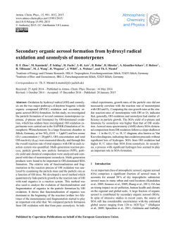
Figure 1: Effective sample size as a function of t,
normalized by the number of PMCMC sweeps (top)
and wall time in seconds (bottom). PGAS with 10
particles is shown in cyan. ICMSC results are shown
in blue, with shorter dashes representing increasing
particle counts 10, 20, 50, 100, 200, and 500. All lines
show the median ESS over 25 independent restarts.
l
p(y N , xkN [x∗,l
n ] | FN [y n , xn ]) as the log-weight of the
l
l
rescored trace R(Tn , Rn−1 ). Note here that by construction, we may extract Tn+1 from Tn without additional computation.
5
Experiments
To evaluate the mixing properties of PGAS relative to
ICSMC, we consider a linear dynamical system (i.e.
a Kalman smoothing problem) with a 2-dimensional
latent space and a D-dimensional observational space,
z t ∼ Norm(A · z t−1 , Q), y t ∼ Norm(C · z t , R).
We impose additional structure by assuming that the
transition matrix A is a simple rotation with angular
velocity ω, whereas the transition covariance Q is a
diagonal matrix with constant coefficient q,
cos ω − sin ω
A=
,
Q = qI 2 .
sin ω
cos ω
We simulate data with D = 36 dimensions, T = 100
time points, ω = 4π/T , q = 0.1, α = 0.1, and r = 0.01.
We now consider an inference setting where C and R
are assumed known and estimate the state trajectory
z 1:T , as well as the parameters of the transition model
ω and q, which are given mildly informative priors,
ω ∼ Gamma(10, 2.5) and q ∼ Gamma(10, 100).
While this is a toy problem where an expectation maximization (EM) algorithm could likely be derived, it
is illustrative of the manner in which probabilistic
programs can extend models by imposing additional
structure, in this case the dependency of A on ω. This
Particle Gibbs with Ancestor Sampling for Probabilistic Programs
Here [...] refers to a vector or matrix literal.
We compare results for PGAS with 10 particles to ICSMC with 10, 20, 50, 100, 200, and 500 particles. In
each case we run 100 PMCMC sweeps and 25 restarts
with different random seeds. To characterize mixing
rates we calculate the effective sample size (ESS) of
the aggregate sample set {wts,l , z s,l
t } over all sweeps
s = {1, . . . , 100},
1
,
k 2
k (Vt )
ESSt = P
Vtk =
L
100 X
X
wts,l I[z kt = z s,l
t ].
s=1 l=1
Vtk
represents the total importance weight assoHere
ciated with each unique value z kt in {z s,l
t }.
Figure 1 shows the ESS as a function of t. ICMSC
shows a decreasing ESS as t approaches 0, indicating
poor mixing for values sampled at early generations.
PGAS, in contrast, exhibits an ESS that fluctuates but
is otherwise independent of t. ESS estimates varied
approximately 15% relative to the mean across independent restarts. This suggests that fluctuations in
the ESS reflect variations in the prior probability of
latent transitions p(z t | z t−1 , A).
For this model, our PGAS implementation with 10
particles has a computational cost per sweep comparable to that of ICSMC with 300 particles. However, when we consider the ESS per computation time,
the increases in mixing efficiency outweigh increases in
computational cost for state estimates below t ' 50.
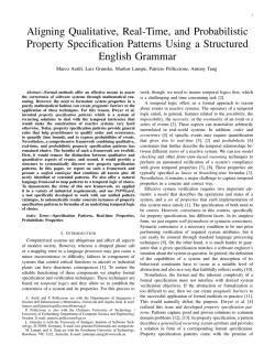
This is further illustrated in Figure 2, which shows
the standard deviation of sample estimates of the parameters ω and q. PGAS shows better convergence per
sweep, particularly for estimates of q. ICSMC with 500
particles performs similarly to PGAS with 10 particles
when estimating ω, though ICSMC with 500 particles
notably has a higher cost per sweep.
0.04
0.04
0.03
0.03
Std[E[q]]
[assume C [...]] ; assumed known
[assume R [...]] ; assumed known
[assume omega (* (sample (gamma-dist 10. 2.5))
(/ pi T))]
[assume A [[(cos omega) (* -1 (sin omega))]
[(sin omega) (cos omega)
]]]
[assume q (sample (gamma-dist 10. 100.))]
[assume Q (* (eye 2) q)]
[assume x
(mem (lambda (t)
(if (< t 1)
[1. 0.]
(sample (mvn-dist (mmul A (x (dec t))) W)))))]
[observe (mvn (mmul C (x 1)) R) [...]]
...
[observe (mvn (mmul C (x 100)) R) [...]]
[predict omega]
[predict q]
Std[E[ω]]
modified Kalman smoothing problem can be described
in a small number of program lines
0.02
0.01
0.00
0
20
40
60
80
100
0.02
0.01
0.00
Sweep
0
20
40
60
80
100
Sweep
Figure 2: Standard deviation of posterior estimates
E[ω] and E[q] over 25 independent restarts, as a function of the PMCMC sweep. PGAS results are shown
in cyan, ICSMC results are shown in blue, with shorter
dashes indicating a larger particle count.
6
Discussion
Relative to other PMCMC methods such as ICSMC,
PGAS methods have qualitatively different mixing
characteristics, particularly for variables sampled early
in a program execution. Implementing PGAS in the
context of probabilistic programs poses technical challenges when programs can make use of recursion and
memoization. The technique for traced evaluation developed here incurs an additional computational overhead, but avoids unnecessary recomputation during regeneration. When the cost of recomputation is large
this will result in computational gains relative to a
naive implementation that re-executes the suffix fully.
Note that our approach tracks upstream, not downstream dependencies. In other words, we know what
environment variables affect the value of a given expression, but not which expressions in a suffix depend on a given variable. All referenced symbol values
must therefore be checked during regeneration, which
can require a O(LN 2 ) computation in itself. Further
gains could be obtained constructing a downstream dependency graph for the suffix, allowing more targeted
regeneration via graph walk techniques analogous to
those employed in Venture [Mansinghka et al., 2014].
At the same time, the empirical results presented here
are indicative of the fact that, even without these additional optimizations, PGAS can easily yield better
statistical results in cases where the parameter space
is large and ICSMC sampling fails to mix.
7
Acknowledgements
The authors would like to thank anonymous reviewers for their comments and Brooks Paige for helpful
discussions. JWM was supported by Google and Xerox. HY was supported by the EPSRC. FW and VKM
were supported under DARPA PPAML. VKM was additionally supported by the ARL and ONR.
Jan-Willem van de Meent,
Hongseok Yang,
References
Christophe Andrieu, Arnaud Doucet, and Roman
Holenstein. Particle Markov chain Monte Carlo
methods. Journal of the Royal Statistical Society:
Series B (Statistical Methodology), 72(3):269–342,
2010.
Pierre Del Moral, Arnaud Doucet, and Ajay Jasra. Sequential Monte Carlo samplers. Journal of the Royal
Statistical Society: Series B (Statistical Methodology), 68(3):411–436, June 2006. ISSN 1369-7412.
doi: 10.1111/j.1467-9868.2006.00553.x.
Noah Goodman, Vikash Mansinghka, Daniel M Roy,
Keith Bonawitz, and Joshua B Tenenbaum. Church:
a language for generative models. In Proc. 24th
Conf. Uncertainty in Artificial Intelligence (UAI),
pages 220–229, 2008.
Pierre E. Jacob, Lawrence M. Murray, and Sylvain
Rubenthaler. Path storage in the particle filter.
Statistics and Computing, December 2013. ISSN
0960-3174. doi: 10.1007/s11222-013-9445-x.
Fredrik Lindsten, Michael I Jordan, and Thomas B.
Sch¨
on. Ancestor Sampling for Particle Gibbs. Neural Information Processing Systems, 2012.
Vikash Mansinghka, Daniel Selsam, and Yura Perov.
Venture: a higher-order probabilistic programming
platform with programmable inference.
arXiv,
page 78, 2014. URL http://arxiv.org/abs/1404.
0099.
T Minka, J Winn, J Guiver, and D Knowles. Infer
.NET 2.4, Microsoft Research Cambridge, 2010.
Brooks Paige and Frank Wood. A Compilation Target
for Probabilistic Programming Languages. International Conference on Machine Learning (ICML), 32,
2014.
Stan Development Team. Stan: A C++ library for
probability and sampling, version 2.5.0, 2014. URL
http://mc-stan.org/.
David Wingate, Andreas Stuhlmueller, and Noah D
Goodman. Lightweight implementations of probabilistic programming languages via transformational
compilation. In Proceedings of the 14th international
conference on Artificial Intelligence and Statistics,
page 770 778, 2011.
F Wood, JW van de Meent, and V Mansinghka. A
new approach to probabilistic programming inference. In Artificial Intelligence and Statistics, pages
1024–1032, 2014.
Vikash Mansinghka,
Frank Wood