1. Art and Diseño

Modern Research in Quantum Physics!
!
!
!
!
!
!
!
!
!
!
!
!
!
!
!
!
!
!
!
!
!
!
A two-level system interacting with electromagnetic
fields near radiating Schwarzschild Black Holes.!
D. Jose Manuel Sánchez Velázquez!
!
4º Grado en Física, Universidad de La Laguna.!
!
Tutor: Dr. D. Daniel Alonso Ramírez!
!
Departamento de Física Fundamental, Experimental, Electrónica y Sistemas.
!
Index!
!
!
!
Abstract!
1!
I.
3!
Motivation and methodology!
II. Notes on Quantum Field Theory in Classical Backgrounds!
4!
1. Quantization in flat space-times!
4!
2. Zero-point energy and the Casimir force!
6!
3. The Hawking radiation!
8!
III. Notes on Quantum Optics!
13!
1. Master equation for a damped two-level atom!
13!
2. Spontaneous emission!
16!
IV. Results and discussion.!
18!
References.!
25
!
Modern Research in Quantum Physics
Abstract!
!
!
!
!
La motivación principal de este trabajo es la formación del alumno en los aspectos
fundamentales de algunas de las teorías fundamentales para comprender la Cosmología, como
son la teoría cuántica de campos y su acoplamiento a espacio-tiempos curvos. Por otro lado se
busca el entendimiento de la interacción radiación-materia, para lo cual se estudiarán los
principios básicos de la Óptica Cuántica tales como la interacción de un sistema de dos niveles
con la radiación monocromática por una parte y con un baño térmico por otro. Esta primera parte
del trabajo más formativa se complementa con el estudio de un artículo científico publicado a
finales de 2013 [1], durante el cual se ponen en práctica las habilidades desarrolladas durante la
etapa formativa.!
!
!
En esta memoria se detallan algunos de los aspectos principales trabajados tanto en
Teoría Cuántica de Campos acoplados a entornos clásicos como en Óptica Cuántica para, a
continuación, exponer y discutir los resultados derivados del análisis del artículo. Se han detallado
algunos cálculos en la medida de lo posible pero se puede encontrar una deducción más completa
de algunos resultados mostrados en las referencias citadas.!
!
!
Comenzamos repasando los principales conceptos de la cuantización de un campo escalar
en un espacio-tiempo plano de Minkowski a partir de la acción que define su evolución dinámica.
Dicha cuantización se lleva a cabo de forma análoga a la que se usa para un sistema finito de
osciladores. A continuación se discute la necesidad de renormalización de la energía de punto
cero para el campo a causa de la divergencia de la misma. A pesar de esta renormalización, se
discute el efecto Casimir debido a la diferencia de energías de punto cero para el campo en
distintas condiciones (se discute el caso de un resonador rectangular).!
!
!
A continuación se discute como generalizar la acción del campo para espacio-tiempos
curvos y los cambios que debemos realizar en la misma para que sea generalmente covariante en
tanto que esto es un requerimiento para que la teoría sea válida en Relatividad General. Esta
sección concluye con la discusión de la denominada radiación Hawking tras obtener los estados
fundamentales del campo para un observador en caída libre y otro observador a una distancia
radial fija en las cercanías de un Agujero Negro de Schwarzschild. Esta discusión se lleva a cabo
en un modelo simplificado en que consideramos un reducción 1+1 dimensional del espacio-tiempo
de Schwarzschild aunque finalmente se comenta el caso más complejo en que se considera el
espacio-tiempo cuadridimensional. !
!
!
La segunda revisión teórica versa sobre algunos principios de la Óptica Cuántica,
centrándonos en la descripción de un sistema de dos niveles acoplado a un baño térmico. Se
discute la obtención de la ecuación maestra y la aproximación de Born-Markov que se utiliza en
este caso. Se obtiene el espectro de emisión espontánea para este sistema usando el teorema de
regresión cuántica para calcular las funciones de correlación necesarias para este fin.!
!
!
Dentro de este análisis se ha procedido a evaluar el espectro de emisión del sistema de
dos niveles para diferentes masas de Agujero Negro y para distintas distancias radiales del
horizonte de sucesos y se discuten los resultados obtenidos en función de la radiación Hawking
emitida por el Agujero Negro. Posteriormente se ha procedido a un análisis del espectro de
fluorescencia resonante del sistema sometido a un campo láser sintonizado en la frecuencia de
transición del mismo. Se discute la variación del mismo con la masa del Agujero Negro para una
potencia determinada del láser. Por tanto, en el análisis del artículo se ponen en práctica tanto la
interacción materia-radiación como la cuantización del campo electromagnético en espaciotiempos curvos. En particular se trabaja sobre la radiación Hawking, la cual se ha descrito durante
el repaso a los aspectos fundamentales trabajados.!
!
1
Modern Research in Quantum Physics
!
Por otro lado, se discute la existencia de isotermas para Agujeros Negros en función de su
masa y de la distancia radial a la que se encuentra el observador, en tanto que la temperatura de
éstos depende de la posición del observador, aumentando para distancias radiales menores,
debido al desplazamiento al rojo inverso gravitacional.!
!
!
Con todo este trabajo se ha pretendido dar una idea más exacta del trabajo que se lleva a
cabo en el terreno de la Física Teórica al alumno y que éste adquiera las habilidades necesarias
para la comprensión de las principales ideas y conceptos desarrolladas en la actualidad, así como
las actuales líneas de investigación que se siguen. Se ha buscado también fomentar la capacidad
analítica de conceptos abstractos y del razonamiento para fenómenos de naturaleza no intuitiva.
2
Modern Research in Quantum Physics
I.
!
!
!
Motivation and methodology!
!
The main purpose of this work is the formation of the student on topics related with the
actual research in Physics by analyzing a recent article on the dynamics of simple quantum
systems interacting with a electromagnetic field near radiating Schwarzschild Black Holes [1].!
!
!
Being my first contact with a very specialized literature, it demanded on first place the study
in depth of the basic theoretical framework of quantum fields in the presence of gravity and
secondly, the study in great detail of some recent published papers.!
!
!
The methodology followed is quite simple, we have studied the different topics from
different sources which are detailed in the references section and have derived every conclusion
rigorously performing every needed operation. For the most practical part of the work which was
the analysis of the paper [1] we used the computational environment MATLAB in order to obtain
the figures showed at the discussion of the results. !
!
!
We have structured this memory as a brief review of all the topics studied during the
realization of the work, starting by the quantization of the electromagnetic field in the presence of
gravity which leads us to the obtention of the emission of particles by Black Holes as the Hawking
radiation. Afterwards, we present the main results studied in Quantum Optics needed for the
discussion of the results obtained after analyzing the paper [1]. Finally we included all the relevant
figures obtained during this analysis and we discuss the results obtained.
3
Modern Research in Quantum Physics
II. Notes on Quantum Field Theory in Classical
Backgrounds!
!
1. Quantization in flat space-times
!
!
We are going to focus on a minimal coupling scheme to take into account the curvature
effects on the quantum fields. We should start by defining how this minimal coupling between the
field and the space-time curvature is achieved. We start by considering the quantization of a field in
the Minkowski flat space-time and then we will generalize this procedure to the general curved
space-times. Finally we will discuss the emission of particles by a Black Hole as described on this
theory.!
!
!
To quantize a free field in a flat space-time we should formally consider it as an infinite set
!
of harmonic oscillators, each one of them fixed at a space position φ ( x,t) → φ x! (t) , so we can
quantize it in the same way it is done for a finite set of harmonic oscillators, the action for the
infinite set of harmonic oscillators can be obtain taking the appropriate limits as:!
!
!
⎤
1 ⎡N 2 N
1
! !
! ! !
!
! !
S[qi ] = ∫ ⎢ ∑ q!i − ∑ M ij qi q j ⎥dt → S[φ ] = ∫ dt ⎡⎣ ∫ d 3 xφ" 2 ( x,t ) − ∫ d 3 xd 3 yφ ( x,t )φ ( y,t ) M ( x, y ) ⎤⎦ ;!
2 ⎣ i=1
2
i, j=1
⎦
in addition, we are going to use a relativistic theory therefore, the action must be invariant under
the transformations of the Poincaré group describing the time and space shifts, spatial rotations
and Lorentz transformations (boosts). The simplest action fulfilling these requirements is:!
!
!
S[φ ] =
( )
1 3 ! ⎡ "2
1
2
d x dt ⎣φ − ( ∇φ ) − m 2φ 2 ⎤⎦ = ∫ d 4 x ⎡⎣η µν ∂ µ φ ( ∂ν φ ) − m 2φ 2 ⎤⎦ ;!
∫
2
2
where η µν = diag(1,−1,−1,−1) is the Minkowski metric and the Greek indices label four-
(
)
!
dimensional coordinates: x 0 ≡ t , x1 , x 2 , x 3 ≡ x . The equation of motion for the field is obtained by
the variational principle:!
!
!
δS
"
!
!
2
! = φ!!( x,t ) − Δφ ( x,t ) + m φ ( x,t ) = 0 .!
δφ ( x,t )
!
However, this equation of motion shows that the oscillators are coupled, so, as in the case
of the finite set, we should decouple them by defining the normal modes which in the infinite set
case are obtained by applying the Fourier transform:!
!
!
d 3 x −ik! ·x! !
e φ ( x,t ) , !
( 2π )3/2
!
d 3k ik! ·x! !
!
φ ( x,t ) ≡ ∫
e φk ( t ) , !
( 2π )3/2
φk! ( t ) ≡ ∫
!
from which are obtained the equations of motion for the (decoupled) normal modes of the field as:!
!
4
Notes on Quantum Field Theory in Classical Backgrounds
Modern Research in Quantum Physics
d2 !
φ ( t ) + ( k 2 + m 2 )φk! ( t ) = 0 .!
dt 2 k
They describe an infinite set of decoupled oscillators with frequencies: ω k ≡
!
k 2 + m 2 .!
!
Once we have the field modes, it is very easy to quantize the field by taking account of the
form of each mode and substituting each amplitude by the creation and annihilation operators:!
!
φk! ( t ) =
(
)
(
)
1
1
ak−! e−iω kt + a−+k! eiω kt → φˆk! ( t ) =
aˆ −! e−iω kt + aˆ−+k! eiω kt ;!
2ω k
2ω k k
!
where the annihilation and creation operators satisfy the same commutation relations than the
harmonic oscillator as:!
!
! !
⎡⎣ aˆ k−! , aˆ k+! ' ⎤⎦ = δ k − k ' ;
(
)
!
⎡⎣ aˆ k±! , aˆ k±! ' ⎤⎦ = 0 .!
!
Taking into account the expression for the mode operator we can write the field operator in
terms of the mode operators:!
!
!
!
3
d
k
!
φˆ ( x,t ) = ∫
( 2π )3/2
! !
! !
1
⎡ aˆ k−! e−iω kt+ik ·x + aˆ k+! eiω kt−ik ·x ⎤ ,!
⎦
2ω k ⎣
relation known as mode expansion of the quantum field. It is remarkable that this mode expansion
is valid for flat space-times. In general, when considering curved space-times, the frequency in the
modes equations of motion is explicitly time-dependent and then the modes are not plane waves
but a mode function υ k! ( t ) satisfying the equation!
!
υ!!k" + ω k2 ( t )υ k" = 0 ;!
!
yielding a more general mode expansion of the quantum field operator of the form!
!
!
3
! !
! !
d
k
1
!
⎡ aˆ k−! υ k*! ( t ) eik ·x + aˆ k+! υ k! ( t ) e−ik ·x ⎤ .!
φˆ ( x,t ) = ∫
3/2
⎦
( 2π ) 2 ⎣
!
!
The vacuum state of the quantum field is defined as the eigenstate of all the annihilation
operators with eigenvalue zero:!
!
aˆ k−! 0 = 0 ,
!
!
∀k !
!
Once the ground state is defined, the Hilbert space of states for the field is built as !in the
many oscillators case. The state with occupation number ns in the mode with momentum ks where
s = 1,2... is an index to enumerate the excited modes which are!
!
( )
ns
⎡
aˆ k+!s ⎤
⎥ 0 .!
n1 ,n2 ,... = ⎢ ∏
⎢ s
ns ! ⎥
⎢⎣
⎥⎦
!
5
Notes on Quantum Field Theory in Classical Backgrounds
!
Modern Research in Quantum Physics
The Hilbert space of states is spanned by the vectors n1 ,n2 ,... for all possible choices of
ns (remember we are dealing with bosons). The quantum Hamiltonian for the field can be written
as:!
!ω
Hˆ = ∫ d 3k k ⎡⎣ 2 aˆ k+! ak−! + δ (3) (0) ⎤⎦ !
2
!
in clear analogy to the case of a finite number of harmonic oscillators.!
!
!
!
2. Zero-point energy and the Casimir force
!
!
!
We can now study the zero-point energy of the field given by!
!
!
1
E0 = 0 Hˆ 0 = δ ( 3) ( 0 ) ∫ d 3kω k .!
2
!
This expression which should describe the lowest energy of the field, however is clearly divergent
as it has an infinite factor δ ( ) ( 0 ) , moreover the integral diverges and can only converge if a proper
upper cut-off frequency is introduced. We need to renormalize the zero-point energy. In order to do
that it is necessary to explain the presence of the divergent factor. If we consider the quantization
of the field in a finite box of volume V [6]:!
3
!
E0 ≈
!
1 V
3
3 ∫ d kω k ,!
2 ( 2π )
!
we can identify the formally divergent factor as the volume of the entire space as it arises when the
box volume grows to infinity. To avoid this divergence we should speak about energy density
instead of energy.!
!
!
!
E0 1 d 3 k
lim
= ∫
ω k .!
V →∞ V
2 ( 2π )3
!
However, this zero-point energy density is still divergent because the integral diverges
!
when k → ∞ , this is called an ultraviolet divergence, because for larger values of the momentum
we obtain larger energies. The formal reason for this divergence is the presence of infinitely many
oscillators φk! ( t ) each one of them with zero-point energy
1
ω k . This is the first of several
2
divergences found in quantum field theory but it is simple to avoid it, in the case of flat space-times,
if we consider the energy of the excited states and that we only can measure differences of
energies between states. The energy of an excited state is written as:!
!
E ( n1 ,n2 ,...) = E0 + ∑ nsω ks ,!
!
s
so it is just the sum of an infinite zero-point energy and a finite state-dependent term which is the
one we can measure due to transition between states, so we can simply subtract this zero-point
6
Notes on Quantum Field Theory in Classical Backgrounds
Modern Research in Quantum Physics
energy and then we can avoid the divergence of energy. After this redefinition the zero-point
energy becomes zero.!
!
!
Although this is a good solution for the energies of excited states there are cases on which
the difference between zero-point energies of different ground states of the field may be important
and produce an actual force. This effect is known as the Casimir effect and has been
experimentally observed [7]. To understand this effect we will focus on the case of a rectangular
resonator and we will obtain an expression for this Casimir force [8].!
!
!
Let us consider the quantization of the field inside a rectangular resonator consistent of two
parallel plates of surface L2 separated a distance a . The zero-point energy in this case is:!
!
E
box
0
1/2
∞
⎡ l 2π 2
!c
π2 ⎤
= ∑ ∑ ⎢ x 2 + ly2 + lz2 2 ⎥
2 pol lx ,ly ,lz ⎣ a
L ⎦
(
)
,!
!
where every mode has two polarization states except those which vanishes that have only one
polarization state. Taking account this fact and considering that the distance between the plates is
much shorter than their longitude, a << L we can replace the summation on l y , lz by integrals and
we can rewrite the energy as:!
!
E
box
0
∞
1/2
∞
∞
!cπ L2
=
d ξ ∫ dζ ⎡⎣lx2 + ξ 2 + ζ 2 ⎤⎦ !
3 ∑ ∑ ∫0
0
2a pol lx =0
!
where we have introduced ξ ≡
ly a
la
and ζ ≡ z . If we introduce the polar coordinates
L
L
ξ = u cosϕ , ζ = u sin ϕ and perform the summation over the polarization states we obtain :!
!
∞ ∞
⎤
!cπ L ⎡ ∞
2
=
⎢ ∫0 du u + 2∑ ∫ du lx + u ⎥ .!
3
2a ⎣
lx =1 0
⎦
2
E
box
0
2
!
!
Following the same procedure for the vacuum in the empty space, we obtain a similar
expression for the zero-point energy:!
!
E0vac =
!cπ 2 L2
4a 3
∫
∞
0
∞
dlx ∫ du lx2 + u .!
!
0
!
Although these two expressions are clearly divergent, the difference between them
converges to a finite number. The only difference between the two considered cases is the
presence of two parallel plates in the resonator and the summation on the l x modes which in empty
space case is an integral as for the l y and lz modes. We calculate the energy difference per
surface unit:!
!
where we have introduced:!
υ = ( E0box − E0vac ) =
!
!cπ 2 !
I ,!
4a 3
!
7
Notes on Quantum Field Theory in Classical Backgrounds
Modern Research in Quantum Physics
∞
∞
∞
∞
∞
∞
1 ∞
1
I! = ∫ du u + ∑ ∫ du lx2 + u − ∫ dlx ∫ du lx2 + u = I ( 0 ) + ∑ I ( l ) − ∫ dlI ( l ) .!
0
0
0
0
2 0
2
lx =1
l=1
!
!
We have to obtain this difference as the divergent part of I! . In order to do that we use the
Euler-McLaurin formula which relates the integral and the summation of an analytic function:!
!
3
∞
∞
!I = 1 I ( 0 ) + ∑ I ( l ) − dlI ( l ) = − 1 B2 dI ( 0 ) − 1 B4 d I ( 0 ) − ... !
∫0
2
2!
dl
4!
dl 3
l=1
!
where the Bernoulli numbers are given by the generating function:!
!
∞
y
yj
=
B
∑ j j! ,
e y − 1 j=0
Evaluating the derivatives:!
!
B2 =
!
1
,
6
B4 = −
1
.!
30
dI ( l )
d 3 I (l )
d n I (l )
= −2l 2 ,
=
−4
,
= 0 ∀n ≥ 4 ,!
dl
dl 3
dl n
!
we see that the difference is actually finite yielding:!
!
1
I! = −
.!
180
!
!
!
So, the energy difference per unit surface is:!
1 !cπ 2
υ (a) = −
,!
720 a 3
!
which produces an attractive force per unit surface on the resonator plates which is expressed
through:!
!
F (a) ≡ −
dυ
π 2 !c
=−
.!
da
240 a 4
!
!
This force, due to the difference between the infinite zero-point energies produces an
attraction between the plates which is larger when the distance between them is shorter. This is
known as the Casimir effect and has been experimentally proved but using a plate and a sphere
because of the difficulty in building a setup of two perfect parallel plates [7].!
!
!
!
3. The Hawking radiation
!
!
As we want to consider a general curved space-time, we must perform some changes in
the action defined before in order to have Poincaré invariant fields and a generally covariant
theory. We must replace the Minkowski metric by the general space-time metric: ηµν → gµν and we
should also replace the spatial derivatives by covariant derivates, however, in the case we are
8
Notes on Quantum Field Theory in Classical Backgrounds
Modern Research in Quantum Physics
considering (a real scalar field) this substitution will make no difference. Finally we must replace
!
the Minkowski volume element by the covariant volume element: d 3 xdt → d 4 x −g where
( )
g ≡ det gµν is the determinant of the covariant metric tensor. Performing these changes we obtain
a generally covariant action for a real scale field:!
!
1
S[φ ] = ∫ d 4 x −g ⎡⎣ g µνφ,µφ,ν − V (φ ) ⎤⎦ ,!
2
!
where φ,µ denotes the derivative of the field with respect to x µ . The modifications performed to the
action are the necessary ones to make it suitable for the General Relativity. This new action
depends on gµν and is coupled to gravity. This form of coupling is called minimal coupling to gravity
as it is the minimal required coupling due to the requirements of General Relativity. The
quantization of the field is done in the same way as above but with different mode functions.!
!
!
!
We will focus only in the conformally flat space-times as they can be easily mapped to the
Minkowski space-time and so the quantization of the fields can be performed in the same way as
shown in previous sections. A conformally flat space-time is the one whose metric can be written
as:!
!
gµν = Ω 2 ( x )ηµν ,!
!
where the conformal factor Ω ( x ) is an arbitrary non vanishing function of space-time.!
!
!
We are specially interested in the quantization of the field in the neighborhood of a
Schwarzschild Black Hole as our case of study will treat a quantum system interacting with the
electromagnetic field in this situation. Let us start by considering the action of the field. The metric
describing the space-time near a Black Hole is the Schwarzschild one but in the derivation we will
present we are going to restrict ourselves to the two dimensional case as the space-time has
spherical symmetry. The main features of our interest will remain and we will consider corrections
when considering four-dimensional space-time.!
!
!
We are then considering the reduction 1+1 of the Schwarzschild space-time to simplify the
mathematical derivations. The reduced metric tensor in the considered case is!
!
!
!
!
⎛
2M
⎜ 1− r
gab = ⎜
⎜
0
⎜
⎝
0
⎛ 2M ⎞
− ⎜ 1−
⎟
⎝
r ⎠
−1
⎞
⎟
⎟;
⎟
⎟
⎠
−1
⎛ 2M ⎞ 2 ⎛ 2M ⎞
2
ds = ⎜ 1−
⎟ dt − ⎜⎝ 1−
⎟ dr .!
⎝
r ⎠
r ⎠
2
The action for a minimally coupled massless scalar field is:!
S[φ ] =
1 ab
g φ,aφ,b −gd 2 x ; a,b = 0,1 ; x 0 ≡ t , x1 ≡ r ;!
2∫
!
this action is conformally coupled to gravity so a significant simplification occurs if we bring the
metric to a conformally flat form. This is achieved by changing the the coordinate r → r * where the
new coordinate is chosen so that:!
!
9
Notes on Quantum Field Theory in Classical Backgrounds
Modern Research in Quantum Physics
⎛ 2M ⎞ *
⎛ r
⎞
dr = ⎜ 1−
dr → r * ( r ) = r − 2M + 2M ln ⎜
− 1⎟ .!
⎟
⎝
⎝ 2M ⎠
r ⎠
!
!
!
In this new coordinates the metric is conformally flat, !
2M ⎞
⎛
ds 2 = ⎜ 1− * ⎟ ⎡⎣ dt 2 − dr 2 ⎤⎦ ,!
⎝ r(r ) ⎠
!
we should remark that the new coordinate is defined only for r < 2M and varies in the range
−∞ < r * < +∞ so an object approaching the horizon needs to travel an infinite coordinate distance,
that is why it is usually called the tortoise coordinate. In the regions far from the Black Hole this
coordinates are asymptotically the same as the Minkowski ones.!
!
!
!
In this new coordinates the action is written as:!
S[φ ] =
(
)
2
1 ⎡
2
⎤dtdr * , !
∂
φ
−
∂
(
)
*φ
t
∫
r
⎢
⎣
⎦⎥
2
!
and the general solution or the equation of motion may be written in the form:!
!
φ ( t,r * ) = P ( t − r * ) + Q ( t + r * ) ,!
!
where P and Q are arbitrary but sufficiently smooth functions. If we consider the light cone
coordinates u ≡ t − r * and v ≡ t + r * :!
!
⎛
2M ⎞
ds 2 = ⎜ 1−
dudv .!
* ⎟
⎝ r (r )⎠
!
!
Those coordinates defined above are good to describe the space-time in the outside of a
Black Hole but they don’t cover the inside of it, so in order to describe the electromagnetic vacuum
in this region we need to use the so-called Kruskal coordinates, which avoid the coordinate
singularity of the Schwarzschild metric at r = 2M by using the appropriate change of coordinates
which yields to a regular metric at the Black Hole horizon. This coordinates describe the spacetime of an free falling observer into the Black Hole so the coordinates will be both the proper time
and proper distance of the free falling observer ( t , r ) . In the light cone coordinates we can relate
the Kruskal coordinates with the tortoise ones. This relation is given by the expressions:!
!
⎛ u ⎞
u = −4M exp ⎜ −
;
⎝ 4M ⎟⎠
!
Using the inverse relations:!
!
⎛ v ⎞
v = 4M exp ⎜
.!
⎝ 4M ⎟⎠
uv ⎞
⎛ u⎞
⎛
t = 2M ln ⎜ − ⎟ ; r * = 2M ln ⎜ −
;!
⎝ v⎠
⎝ 16M 2 ⎟⎠
!
we can rewrite the metric in terms of the Kruskal coordinates in the light cone:!
!
ds 2 =
2M
⎛ r(u,v ) ⎞
exp ⎜ 1−
⎟ dudv .!
⎝
r(u,v )
2M ⎠
10
Notes on Quantum Field Theory in Classical Backgrounds
Modern Research in Quantum Physics
!
!
The Kruskal space-time so defined is the extension of the Schwarzschild space-time
spanned by the Kruskal coordinates to their maximal ranges. Since the Kruskal metric is
conformally flat the general solution for the field is of the form:!
!
φ (u,v ) = A ( u ) + B ( v ) .!
!
!
It is remarkable that a free falling observer in this coordinates has proper acceleration zero
but an observer at a fixed radial distance from the Black Hole must has a proper acceleration.!
!
!
We can quantize the field in the two coordinates systems. It is convenient to do so in the
light cone mode expansions. Then we have:!
!
φ (u,v) = ∫
∞
φ (u,v ) = ∫
∞
0
!
0
dΩ
2π
dω
2π
1
⎡ e−iΩu bˆΩ− + eiΩu bˆΩ+ + e−iΩvbˆ−−Ω + eiΩvbˆ−+Ω ⎤ ;!
⎦
2Ω ⎣
1
⎡ e−iω u aˆω− + eiω u aˆω+ + e−iω v aˆ−−ω + eiω v aˆ−+ω ⎤⎦ ;!
2ω ⎣
each set of operators {aˆ ±±ω } , {bˆ±±Ω } define a different vacuum state for the field: the Kruskal
vacuum and the Boulware vacuum respectively:!
!
!
aˆ ±−ω 0 K = 0 ; bˆ±−Ω 0 B = 0 .!
!
Now, we have to discuss the relation between vacuum states for each mode expansions.
The importance to do this is that for different observers the mode expansion differs due to the
space-time geometry. This relation is given by Bogolyubov transformations [6] which in the more
general case is written as:!
!
∞
bˆΩ− = ∫ dω ⎡⎣α ωΩ aˆω− + βωΩ aˆω+ ⎤⎦ !
0
!
where α ωΩ and βωΩ are the so-called Bogolyubov coefficients, given by the expression:!
!
Ω
F (ω ,Ω ) ;
ω
α ωΩ =
F (ω ,Ω ) = ∫
∞
−∞
βωΩ =
!
du ⎡
ω
⎤
iΩu + i e− au ⎥ ;
⎢
2π ⎣
a
⎦
Ω
F ( −ω ,Ω ) ;!
ω
ω >0; Ω >0. !
!
!
The vacuum state for the electromagnetic field in the presence of a Black Hole is the
Kruskal vacuum [4] so we might asked for the number of particles measured by an observer at a
fixed radial distance since its vacuum state is the Boulware one:!
!
−1
2
Ω
2
⎡
⎛ 2πΩ ⎞ ⎤
Nˆ Ω ≡ 0 K bˆΩ+ bˆΩ− 0 K = ∫ dω βωΩ = ∫ dω F ( −ω ,Ω ) = ⎢ exp ⎜
− 1 δ ( 0 ) ;!
⎝ 4M ⎟⎠ ⎥⎦
ω
⎣
!
this quantity is divergent as we are considering the entire space but if we concern about the
density of particles:!
!
11
Notes on Quantum Field Theory in Classical Backgrounds
Modern Research in Quantum Physics
−1
⎡
⎛ 2πΩ ⎞ ⎤
nΩ = ⎢ exp ⎜
− 1 ;!
⎝ 4M ⎟⎠ ⎥⎦
⎣
!
in units in which energy is equivalent to frequency, the above formula is equivalent to the BoseEinstein distribution:!
!
−1
⎡
⎛ E⎞ ⎤
n(E) = ⎢ exp ⎜ ⎟ − 1⎥ !
⎝ TH ⎠ ⎦
⎣
!
where we have defined the Hawking temperature of the Black Hole which arises from the thermal
spectrum an observer at long radial distances will measure. For observers closer to the Black Hole,
the temperature will be higher due to the inverse gravitational redshift:!
!
TH =
!c 3
.!
8π GMkB g00
!
!
If we had considered the four dimensional case, the basics results would have remained
but we should have taken into account a field decomposition into spherical harmonics:!
!
φ ( t,r,θ ,ϕ ) = ∑ φlm ( t,r )Ylm (θ ,ϕ ) .!
l,m
!
!
If we consider only the spherically symmetric mode, the solution would be almost equal to
the one obtained in the 1+1 dimensional case but the distribution of measured particles would
decrease with respect with the one previously obtained. This decrease of the intensity is taking into
account by introducing the greybody factor, whose expression is explicitly given in [1].!
!
12
Notes on Quantum Optics
Modern Research in Quantum Physics
III. Notes on Quantum Optics!
!
1. Master equation for a damped two-level atom
!
!
The damped two-level atom will provide us an elementary description of the interaction of
the atom with an electromagnetic field. We will restrict ourselves to the purely radiative damping
case considering that the collisions between atoms are negligible. We consider an atom with two
states: 1 and 2 with respective energies E1 , E2 with E1 < E2 . Our objective is to describe the
energy dissipation through the coupling of both states with the many modes of an electromagnetic
field. !
!
!
The treatment of the system may be done using the Pauli spin operators. Let’s start by
remembering the representation of an operator in terms of a complete set of states { n } :!
!
Oˆ = ∑ n Oˆ m n m ,!
!
n,m
if we use as the complete set the two states of our system, we can write the Hamiltonian as:!
!
H A = E1 1 1 + E2 2 2 =
1
1
E1 + E2 ) Iˆ + ( E2 − E1 )σ z ,!
(
2
2
!
where σ z ≡ 2 2 − 1 1 . There exist other two important operators for this system: the atomic
lowering and raising operators: σ − ≡ 1 2 , σ + ≡ 2 1 .!
!
!
The first term in the Hamiltonian is a constant and might be removed by redefining our
energy reference as the middle of the atomic transition:!
!
HA =
!
1
!ω Aσ z ;
2
ωA ≡
E2 − E1
.!
!
!
As we want to know how the atom interacts with the environment, we need to modulate it.
In order to do that we start by considering the total Hamiltonian of the system interacting with an
environment modeled as a collection of harmonic oscillators:!
!
H = H A + H R + H I ;!
!
H A ≡ atom Hamiltonian; H R ≡ reservoir Hamiltonian; H I ≡ atom-reservoir interaction Hamiltonian.!
!
!
!
Those Hamiltonians have the explicit expression!
H=
(
)
1
!ω Aσ z + ∑
!ω k rk!†,λ rk! ,λ + ∑
! κ k*! ,λ rk!†,λσ − + κ k! ,λ rk! ,λσ + ;!
!
!
2
k ,λ
k ,λ
!!
ωk ! !
κ k! ,λ ≡ −ieik ·rA
eˆ ·d21 .!
2!ε 0V k ,λ
!
!
This is the full Hamiltonian of both
! the system and the reservoir where the summation is
extended to all wave number vectors k and polarization states λ . The atom position is denoted by
13
Notes on Quantum Optics
Modern Research in Quantum Physics
!
rA , eˆk! ,λ is a unitary vector in the polarization direction and V is the quantization volume. κ k! ,λ is
called the dipole coupling constant.!
!
!
The reservoir is only of indirect interest and we only need to specify some of its properties
in a general way. We are seeking information about the system without having the total information
about the composite system S ⊕ R so we define the reduced density operator through the total
density operator as:!
!
ρ ( t ) = trR ⎡⎣ χ ( t ) ⎤⎦ , !
!
being ρ ( t ) the reduced density matrix, χ ( t ) the density matrix of the composite system and the
trace is taken over the reservoir states. If we consider an operator of the Hilbert space of the
system S , its average will be:!
!
{
}
ˆ ⎡ χ ( t ) ⎤ = tr ⎡Oˆ ρ ( t ) ⎤ ,!
Oˆ = trS⊕R ⎡⎣Oˆ χ ( t ) ⎤⎦ = trS Otr
R⎣
S ⎣
⎦
⎦
!
so we just need to obtain an equation for ρ ( t ) into R .!
!
!
We shall start from the more general expression for the evolution of the density operator
and then perform some approximations. The Schrödinger equation for the density operator is:!
!
χ! =
!
1
[H , χ ] ,!
i"
which can be written in the interaction picture as we know the solution for both the free system and
the free reservoir Hamiltonians. Defining the density operator in the interaction picture:!
!
i
χ! ≡ e "
( H A +H R )t
H! I ≡ e
we obtain:!
!
χ (t ) e
i
( H A +H R )t
"
i
− ( H A +H R )t
"
HIe
!
i
− ( H A +H R )t
"
,!
!
i
i
( H A +H R )t
− ( H A +H R )t
i
i
1
χ!" = ( H A + H R ) χ! − χ! ( H A + H R ) + e #
χ" e #
= [ H! I ( t ) , χ! ] ;!
#
#
i#
!
expression that can be written, after formally integrating χ!" and replacing into the commutator, as
follows:!
!
1
1 t
χ!" = ⎡⎣ H! I (t), χ ( 0 ) ⎤⎦ − 2 ∫ dt ' ⎡⎣ H! I ( t ) , ⎡⎣ H! I ( t ') , χ! ( t ') ⎤⎦ ⎤⎦ .!
i#
# 0
!
!
So far we only have expressed the original equation in a more convenient form to perform
the two approximations needed to obtain the master equation: the Born-Markov approximation. We
will asume that the interaction between the system and the reservoir is turned on at t = 0 and that
there is no correlation between them at this time, then:!
!
χ (0) = ρ ( 0 ) R0 ;!
!
14
Notes on Quantum Optics
Modern Research in Quantum Physics
where R0 is the initial reservoir density operator. Noting that trR ⎡⎣ χ! ( t ) ⎤⎦ ≡ ρ! ( t ) and assuming that !
trR ⎡⎣ H! I ( t ) R0 ⎤⎦ = 0 (this is always possible after a proper redefinition of the full Hamiltonian) we
obtain the master equation for the reduced density operator after tracing over the reservoir states:!
!
{
}
1 t
ρ!" = − 2 ∫ dt 'trR ⎡⎣ H! I ( t ) , ⎡⎣ H! I ( t ') , χ! ( t ') ⎤⎦ ⎤⎦ ;!
# 0
!
!
Despite χ! factorizes at the initial time, this is no longer true at later times as correlations
between the system and the reservoir will arise. However, we are considering that the coupling
between the system and the reservoir is very weak, so at all times the density operator will show
only deviations of the order H I from the uncorrelated state. Moreover, as the reservoir state may
remain unaltered by the system, we can approximately write:!
!
χ! ( t ) = ρ! ( t ) R0 + O ( H I ) .!
!
!
Once we have this expression we are able to do our first important approximation and
neglect terms higher than those of second order in H I . This is called the Born approximation and it
allows us to write the master equation as:!
!
{
}
1 t
ρ!" = − 2 ∫ dt 'trR ⎡⎣ H! I ( t ) , ⎡⎣ H! I ( t ') , ρ! ( t ') R0 ⎤⎦ ⎤⎦ .!
# 0
!
!
Our second approximation is the so-called Markov approximation and it states that the
future evolution of the system depends only on its present state and not on its past history. In this
sense the equation above doesn’t fulfill this requirement as the time evolution depends on the
values of the reduced density operator at past times. The statement that the system must be
Markovian is based in the idea that the only information about the past states of the system are in
its coupling with the reservoir, but, as the reservoir doesn’t change its state because of the
interaction, it doesn’t reflect the history of the system so it future evolution can’t depend on its
earlier states. Performing this approximation we have for a general system coupled to a reservoir
the master equation in the Born-Markov approximation.!
!
{
}
1 t
ρ!" = − 2 ∫ dt 'trR ⎡⎣ H! I ( t ) , ⎡⎣ H! I ( t ') , ρ! ( t ) R0 ⎤⎦ ⎤⎦ .!
# 0
!
!
If we consider the particular case in which the system is the two-level atom considered at
the beginning of this section and that the reservoir is a thermal bath we can obtain, after
performing the necessary calculations [3], the master equation for a radiatively damped two-level
atom.!
!
R0 ≡ ∏ e
−
!ω j rj†rj
kBT
j
!ω j
⎛
⎞
−
kBT
⎜ 1− e
⎟ ;!
⎝
⎠
i
γ
γ
ρ! ( t ) = − ω ' A [σ z , ρ ] + ( n + 1) ( 2σ − ρσ + − σ +σ − ρ − ρσ +σ − ) + n ( 2σ + ρσ − − σ −σ + ρ − ρσ −σ + ) ;!
2
2
2
!
where n ≡ n (ω ,T ) is the number of photons with frequency ω :!
!
15
Notes on Quantum Optics
Modern Research in Quantum Physics
n (ω ,T ) =
e
−
!ω
kBT
−
!ω
kBT
;!
1− e
ω ' A is the transition frequency taking account of the Lamb shift, which includes a temperaturedependent term:!
!
ω LS
ω ' A ≡ ω A + ω LS ;!
!
!
2
g
k
κ
k,
λ
!
⎛ !kc ⎞
= ∑ P ∫ d 3k
coth ⎜
;!
ω A − kc
⎝ 2kBT ⎟⎠
λ
() ( )
and γ is the damping constant defined by:!
!
!
! !
!
2
γ ≡ 2π ∑ ∫ d 3kg k κ k, λ δ ( kc − ω A ) .!
λ
() ( )
!
!
The most important result of this section is that the emission and absorption rates of the
two-level atoms are not equal but the emission one will be always larger than the absorption one.
As we can see from the master equation, the emission rate is proportional to n + 1 but the
absorption one is proportional to n . So the emission process 2 → 1 has two components, the
one due to he spontaneous emission which doesn’t depend on the thermal radiation and another
component which describes a rate of stimulated transitions due to the thermal radiation, but the
absorption process 1 → 2 has only the thermal radiation-dependent term as it needs energy to
occur.!
!
!
!
2. Spontaneous emission
!
!
!
The mean values of the two-level operators are related with the reduced density matrix
elements as:!
!
σ z = ρ 22 − ρ11 ;
σ − = ρ 21 ;
!
σ + = ρ12 .!
!
Using the master equation written before, we can easily obtain the equation of motion of
each reduced density matrix element and the equation of motion of the mean values of the
operators:!
!
σ! z = −γ ⎡⎣ σ z ( 2n + 1) + 1⎤⎦ ,!
⎡γ
⎤
σ! − = − ⎢ ( 2n + 1) + iω A ⎥ σ − ,!
⎣2
⎦
⎡γ
⎤
σ! + = − ⎢ ( 2n + 1) − iω A ⎥ σ + ;!
⎣2
⎦
!
!
As we are interested in the spontaneous emission spectrum of the atom, we have to
calculate the following expression which give us the probability of detect a photon of frequency ω
during the interval t = 0 to t = T [3]:!
!
16
Notes on Quantum Optics
Modern Research in Quantum Physics
P (ω ) ∝ ∫ dt ∫ dt 'e−iω (t−t ') σ + ( t )σ − ( t ') .!
T
T
0
0
!
We need to calculate the correlation function σ + ( t )σ − ( t ') and in order to do that we will
!
use the quantum regression theorem which allows us to calculate easily the correlation function
equation of motion from the mean values operators ones. A complete description of this theorem
can be found in chapter 1 of [3]. Applying this theorem we start by writing the mean values
equations of motion in vector form:!
!
⎛ σ−
d ⎜
σ+
dt ⎜
⎜ σ +σ −
⎝
!
⎞
⎟
⎟
⎟
⎠
⎛ ⎛γ
⎞
⎜ − ⎜⎝ + iω A ⎟⎠
2
⎜
⎜
=⎜
0
⎜
⎜⎝
0
⎞
0 ⎟
⎟
⎟
0 ⎟
⎟
−γ ⎟⎠
0
⎛γ
⎞
− ⎜ − iω A ⎟
⎝2
⎠
0
!
⎛ σ−
⎜
⎜ σ+
⎜ σ +σ −
⎝
⎞
⎟
⎟
⎟
⎠
.!
Now, for the correlation function we are interested in:!
!
d
dτ
⎛ σ (t + τ )
−
⎜
σ + (t ) ⎜ σ + (t + τ )
⎜
⎝ σ +σ − ( t + τ )
⎞
⎟
⎟
⎟
⎠
⎛ ⎛γ
⎞
⎜ − ⎜⎝ + iω A ⎟⎠
2
⎜
=⎜
0
⎜
⎜
⎜⎝
0
σ + ( t )σ ( t + τ ) = e
−iω Aτ
e
−(γ /2 )τ
!
e
−γ t
⎞
0 ⎟
⎛ σ (t + τ )
−
⎟
⎜
⎟ σ + (t ) ⎜ σ + (t + τ )
0 ⎟
⎜
⎟
⎝ σ +σ − ( t + τ )
−γ ⎟⎠
0
⎛γ
⎞
− ⎜ − iω A ⎟
⎝2
⎠
0
!
→ σ ( t )σ ( t ') = e
!
+
−iω A ( t−t ') −(γ /2 )( t+t ')
e
⎞
⎟
⎟
⎟
⎠
;!
!
!
Substituting this expression in the integral we obtain the spontaneous emission spectrum if
we consider time intervals long enough we obtain a Lorentzian line shape:!
!
P (ω ) ∝
1
2
⎛γ ⎞
⎜⎝ ⎟⎠ + (ω − ω A )
2
2
.
17
Modern Research in Quantum Physics
IV. Results and discussion.!
!
!
As a practical case of application of the skills acquired during the development of the work
we have analyzed a recent article [1]. In this paper it is discussed how the density matrix of a twolevel system of transition frequency ω 0 is varied by the influence of space-time curvature near the
horizon of a radiating Schwarzschild Black Hole. The reduced density matrix for the two-level
system is [1]:!
!
⎛
Γ(−ω 0 )
− Γ t (ω 0 )τ
+
1− e− Γt (ω 0 )τ
⎜ ρ 22 (0)e
Γ t (ω 0 )
ρ (t) = ⎜
⎜
− Γ t (ω 0 )τ 2 +iΩτ
ρ
0
e
(
)
12
⎜
⎝
(
)
ρ 21 ( 0 ) e
ρ11 (0)e− Γt (ω 0 )τ +
!
− Γ t (ω 0 )τ 2 −iΩτ
(
Γ(ω 0 )
1− e− Γt (ω 0 )τ
Γ t (ω 0 )
)
⎞
⎟
⎟;!
⎟
⎟
⎠
which is obtained after solving the quantum Liouville equation [1], which in the weak coupling limit
between the system and the thermal bath induced by a fluctuating vacuum electromagnetic field
outside a radiating Schwarzschild Black Hole is:!
!
d
1
1
⎛
⎞
⎛
⎞
ρ (τ ) = −i ⎡⎣ H A + H LS , ρ (τ ) ⎤⎦ + Γ ( −ω 0 ) ⎜ ρ11 2 2 − { 1 1 , ρ (τ )}⎟ + Γ (ω 0 ) ⎜ ρ 22 1 1 − { 2 2 , ρ (τ )}⎟ ; !
⎝
⎠
⎝
⎠
dτ
2
2
!
where Γ(ω 0 ) is the emission rate, Γ ( −ω 0 ) is the absorption rate of the electromagnetic field, Ω is
the transition frequency taking into account the Lamb shift H LS and Γ t (ω 0 ) = Γ (ω 0 ) + Γ ( −ω 0 ) .!
!
!
!
We have focussed the analysis on the variation of the spontaneous emission of the system
using the transition rates provided by this paper although the scope of the paper is to search for a
suitable experimental setup to prove the existence of Hawking radiation by the analogy of the
behavior of the two level system near a dielectric body at a finite temperature with the one it has
near a Black Hole. Our interest in this work is just the transition rates and the theoretical study of
properties of the system near the Black Hole horizon.!
!
!
We can only perform calculations for the two asymptotic regions: near the horizon
( r → 2M ) and for large distances from the black hole ( r → ∞ ). In this cases it is possible to
compute analytically each transition rate and so for the total transition rate we obtain:!
!
⎧
2
⎡
⎤
⎞ ⎛ a (r )⎞
⎪ Γ 0 (ω 0 ) ⎢⎛⎜ 1+ 2 πω 2κ
1+
+ f (ω 0 ,2M ) ⎥
⎟
2 ⎟
⎜
0
r
− 1⎠ ⎝
ω0 ⎠
⎪
⎣⎝ e
⎦
Γ t (ω 0 ) ≈ ⎨
2
⎡ ⎛
⎤
⎪
⎞
Γ 0 (ω 0 ) ⎢1+ ⎜ 1+ 2 πω 0 κ r
f (ω 0 ,r ) ⎥
⎟
⎪
− 1⎠
⎣ ⎝ e
⎦
⎩
r → 2M
!
r→∞
!
where!
a (r ) =
r2
M
1− 2M
!
!
r
is the proper acceleration of the static system at position r and 18
Results and conclusions
Modern Research in Quantum Physics
!
f (ω ,r) =
(
3
l l + 1) ( 2l + 1) Tl ω g00
4 4 ∑ (
8r ω l
!
)
2
!
is the so-called grey-body factor which only has an analytical function describing it for the limit
cases of high and low frequencies: M ω << 1 ; M ω >> 1 [2]. Near the horizon the first condition is
always fulfilled so we can use the approximation:!
!
2
f (ω ,r) ∝ g00
M 4 ⎛ 2M ⎞ M 4
= ⎜ 1−
!
⎟
r4 ⎝
r ⎠ r4
which tends to zero in both asymptotical cases.!
!
!
!
Now we have the total transition rate and the reduced density matrix, we can use the
quantum regression theorem[3] to obtain the spectrum of systems close to the horizon and
compare it for different radii and black hole masses. We start by calculating this spectrum:!
!
P (ω ) ∝ ∫ dt ∫ dt 'e−iω (t−t ') σ + ( t )σ − ( t ') ; !
T
T
0
0
σ + ( t )σ − ( t + τ ) = e
P (ω ) ∝
!
−iω 0τ
!
e
⎛ Γ (ω ) ⎞
−⎜ t 0 ⎟ τ
⎝ 2 ⎠
e−( Γt (ω 0 ))t ; !
1
2
⎛ Γ t (ω 0 ) ⎞
⎜⎝
⎟⎠ + (ω − ω 0 )
2
2
;!
!
where n is the mean number of photons with frequency ω 0 which is given by the expression:!
!
ω0
n (ω 0 ,T ) = ⎛ e T − 1⎞
⎝
⎠
−1
!
−1
⎛ 2 πω 0
⎞
= ⎜ e κ r − 1⎟ ; !
⎝
⎠
taking into account that the Hawking temperature for the radiating Black Hole is given by the
expression:!
!
T=
κr
1
=
;!
2π 8π M g00
!
being κ r the superficial gravity of the Black Hole. Once we have the expression for the emission
line of our two-level system, we can discuss it behavior in different situations. We start by plotting
this spectral line at a typical transition energy of 1eV for different Black Hole masses. In order to do
this, we have used the computational environment MATLAB where we have implemented the
necessary code to obtain the following figures on which we will focus our discussion.!
!
!
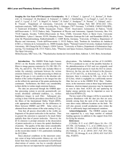
In figure 1 we can observe the spectral line for both asymptotic cases, the radial distance
going to infinite and a fixed radial distance near the horizon (in this case we have chosen this
distance as 1,4nm for reasons we will see later) and its dependence with the Black Hole mass. It is
clear there is a dependence between the width at half height of the spectral line and the mass but
maybe not the most intuitive one since the maximum width is obtained for the lowest massive
Black Holes and in the limit of supermassive Black Holes the resulting spectral line coincide with
the one for the infinite radial distance.!
19
Results and conclusions
Modern Research in Quantum Physics
!
Spontaneous emission
Long radial distance
2.5 solar masses
5 solar masses
10 solar masses
r = 1, 4nm
0
5
10
15
20
Wavelength (mm)
25
30
35
40
Figure 1. Spontaneous emission spectrum for a two-level system located at 1,4 nm of radial
distance from the Black Hole horizon for different Black Hole masses.
!
One might have expected the opposite result but let us analyze qualitatively this result. We
know that the absorption rate of our system contains the effects of the Schwarzschild Black Hole
and this rate is responsible of the enhancement of the line width. So the more intense the radiation
the larger the width and as we know the intensity of the radiation for a given frequency rises with
the temperature of the source which in the present case is the Black Hole. The temperature of the
Black Hole measured by an observer is given by the relation obtained by S.W. Hawking [4]:!
!
!c 3
TH =
!
8π GkB M g00
!
which is inverse to the mass, so the Hawking radiation’s intensity decreases when the Black Hole
mass increases and so the absorption rate or the system decreases. That’s why the width of the
line goes larger for smaller masses.!
!
!
!
Another interesting case of study may be the dependence of the width at half height with
the radial distance to the horizon but taking account of the limitation that we have an approximate
total rate for the limit case when the radial distance to the Schwarzschild Black Hole is almost zero.
For larger distances we might have an analytical function for the transmission coefficient. In figure
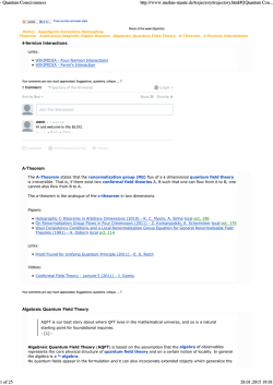
2 we can see that the larger the distance the smaller the width. In this case this dependence is
related with the gravitational redshift and the fact that an observer closer to the Black Hole will see
a higher temperature of it and then the thermal spectrum due to it will be different for each radial
distance as can be seen in figure 3.!
!
!
20
Results and conclusions
Modern Research in Quantum Physics
Spontaneous emission for different radial distances from the horizon
1 nm
10 nm
100nm
1 µm
0
5
10
15
20
Wavelength (mm)
25
30
35
40
Figure 2. Spontaneous emission spectrum for a two-level system in the neighborhood of a 2,5 solar
masses black hole for different radial distances from the horizon.
Emission of a Black Hole of 2.5 solar masses
1 nm
10 nm
100nm
1 µm
0
50
100
150
200
250
Wavelength (mm)
300
350
400
450
500
Figure 3. Spectrum of the Hawking radiation for a 2.5 solar masses Black Hole for different radial
distances from the horizon normalized to observe the variation of the energy at which we can find
the maximum emission.
21
Results and conclusions
Modern Research in Quantum Physics
!
As the maximum of the emission shifts to lower energies as the radial distance grows
larger, the absorption of the two-level system varies and then the spectral line width varies too. So
as we have seen there exist both radial distance and Black Hole’s mass dependence in the
spontaneous emission as there exist the same dependence for the thermal spectrum of the
Hawking radiation.!
!
!
We have spoken about the Hawking radiation and the temperature of the Black Hole so we
can discuss some general features. Let us start by considering the isotherms for a set of Black
Holes, i.e., discussing the radial distance an observer might be at to measure the same
temperature for different Black Hole masses. It is obvious that for higher temperatures the observer
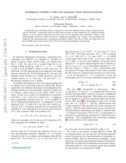
must be closer to the horizon and as can be seen in figure 4 there exist a limit for the radial
distance a observer can be. This limit coincide with the horizon. More attention should be paid to
the long distance limit. We can see that for each isotherm there is a limiting mass so for smaller
masses the Black Hole can’t be colder, but there is no upper limit for the temperature so far.
Black Hole isotherms
10
10 nK
15 nK
25 nK
100 nK
9
Black Hole mass (solar masses)
8
7
6
5
4
3
2
1
0
0
10
20
30
40
50
60
Radial distance (km)
70
80
90
100
Figure 4. Isotherms for different masses and radial distances. It gives us the radial distance an
observer may be at to measure the same temperature for different Black Holes, depending on their
mass.
22
Results and conclusions
Modern Research in Quantum Physics
!
!
!
Once we have discussed he spontaneous emission spectrum, we turn our attention to the
emission of the system when it is placed at a laser field, i.e. the resonance fluorescence spectrum.
We have special interest in the sidebands due to coherent single-mode fields found by Mollow in
the 1960s [5] and it dependence with the presence of the Black Hole.!
!
!
The expression to obtain this spectrum can be found on [5] and we aren’t deriving it here,
but just giving the expression:!
!
Y
1
1 Y2
1+ Y 2
P (ω ) ∝
−
4 ⎛ Γ t (ω 0 ) ⎞ 2
8 (1+ Y 2 )2
2
⎜⎝ 2 ⎟⎠ + (ω − ω 0 )
−
2
1 Y
8 (1+ Y 2 )2
⎡
2
2 Γ t (ω 0 ) ⎤
⎢1− Y + (1− 5Y ) 4δ ⎥
⎣
⎦ −!
2
2
⎛3
⎞
⎜⎝ Γ t (ω 0 )⎟⎠ + (ω − ω A − δ )
4
⎡
2
2 Γ t (ω 0 ) ⎤
⎢1− Y − (1− 5Y ) 4δ ⎥
⎣
⎦ ,!
2
2
⎛3
⎞
⎜⎝ Γ t (ω 0 )⎟⎠ + (ω − ω A + δ )
4
!
where:!
!
δ=
Γ t (ω 0 )
1− 8Y 2 ;
4
Y≡
!
2Ω R
d
; Ω R ≡ 2 E .!
Γ t (ω 0 )
!
!
Ω R is the so-called Rabi frequency and is the frequency at which the atom periodically
cycles between its lower and upper state, following the absorption from the laser field with
stimulated emission and absorption again, and so on.!
!
!
!
!
!
!
!
n 2
n +1 1
n −1 2
n 1
Figure 5. Energy transitions between dressed states that can explain the fluorescence spectrum.
!
!
!
This fluorescence spectrum is due to the transitions between the dressed states as has
been stated by Cohen-Tannoudji [9] and can be seen on the figure 5. Using this model, the
transition frequencies between the shifted states correspond to the ones measured:!
!
!
!
!
!
!
!
!
23
Results and conclusions
Modern Research in Quantum Physics
Resonance fluorescence
Long radial distance
2.5 solar masses
5 solar masses
10 solar masses
0
5
10
15
20
Wavelength (mm)
25
30
35
40
Figure 6. Resonance fluorescence spectrum for a two-level system with a quantum Rabi oscillation
frequency Ω R = 5 MHz at a fixed radial distance of 0.74 nm from the horizon for different Black Hole
masses.
!
!
As we can see on figure 6, the fluorescence spectrum is highly dependent on the mass of
the Black Hole and, as in the spontaneous emission spectrum, the effect of the Black Hole is more
evident for smaller masses than for the greater ones. The most evident case is the one for the 2.5
solar masses Black Hole in which there are no even the sidebands but only a smooth wide peek.
This mass dependence is related with the Hawking radiation and the increase of the absorption
rate of the electromagnetic field by the system.!
!
!
!
!
!
!
!
!
!
!
24
Modern Research in Quantum Physics
References.!
!
[1] J. Hu, W. Zhou, H. Yu, Phys. Rev. D 88, 085035 (2013).!
[2] R. Fabri, Phys. Rev. D 12, 933 (1975).!
[3] H.J. Carmichael, Statistical Methods in Quantum Optics 1 (Springer-Verlag, 1999).!
[4] S.W. Hawking, Nature 248, 30 (1974).!
[5] B.R. Mollow, Phys. Rev. 188 1969 (1969).!
[6] V.F. Mukhanov, S. Winitzki, Introduction to Quantum Fields in Classical Backgrounds
(Cambridge University Press, 2007). !
[7] S.K. Lamoreaux, Phys. Rev. Let. 78, 5 (1997).!
[8] W.P. Schleich, Quantum Optics in Phase Space (Wiley-VCH, 2001).!
[9] C. Cohen-Tannoudji, S. Reynaud, J. Phys. B 10, 345 (1977)
25