
state of the climate in 2015
STATE OF THE CLIMATE IN 2015 Special Supplement to the Bulletin of the American Meteorological Society Vol. 97, No. 8, August 2016 STATE OF THE CLIMATE IN 2015 Editors Jessica Blunden Derek S. Arndt Chapter Editors Howard J. Diamond A. Johannes Dolman Robert J. H. Dunn Dale F. Hurst Gregory C. Johnson Jeremy T. Mathis Ademe Mekonnen A. Rost Parsons James A. Renwick Jacqueline A. Richter-Menge Ahira Sánchez-Lugo Carl J. Schreck III Sharon Stammerjohn Kate M. Willett Technical Editors Kristin Gilbert Tom Maycock Susan Osborne Mara Sprain American Meteorological Society Cover credits: Front : Reproduced by courtesy of Jillian Pelto Art/University of Maine Alumnus, Studio Art and Earth Science — Landscape of Change © 2015 by the artist. Back: Reproduced by courtesy of Jillian Pelto Art/University of Maine Alumnus, Studio Art and Earth Science — Salmon Population Decline © 2015 by the artist. Landscape of Change uses data about sea level rise, glacier volume decline, increasing global temperatures, and the increasing use of fossil fuels. These data lines compose a landscape shaped by the changing climate, a world in which we are now living. (Data sources available at www.jillpelto.com/landscape-of-change; 2015.) Salmon Population Decline uses population data about the Coho species in the Puget Sound, Washington. Seeing the rivers and reservoirs in western Washington looking so barren was frightening; the snowpack in the mountains and on the glaciers supplies a lot of the water for this region, and the additional lack of precipitation has greatly depleted the state’s hydrosphere. Consequently, the water level in the rivers the salmon spawn in is very low, and not cold enough for them. The salmon are depicted swimming along the length of the graph, following its current. While salmon can swim upstream, it is becoming more of an uphill battle with lower streamflow and higher temperatures. This image depicts the struggle their population is facing as their spawning habitat declines. (Data sources available at www.jillpelto.com/salmon-populagtion-decline; 2015.) How to cite this document: Citing the complete report: Blunden, J. and D. S. Arndt, Eds., 2016: State of the Climate in 2015. Bull. Amer. Meteor. Soc., 97 (8), S1–S275. Citing a chapter (example): Mekonnen, A., J. A. Renwick, and A. Sánchez-Lugo, Eds., 2016: Regional climates [in “State of the Climate in 2015”]. Bull. Amer. Meteor. Soc., 97 (8), S173–S226. Citing a section (example): Tsidu, M., 2016: Southern Africa between 5° and 30°S [in “State of the Climate in 2015”]. Bull. Amer. Meteor. Soc., 97 (8), S192–S193. EDITOR AND AUTHOR AFFILIATIONS (alphabetical by name) Aaron-Morrison, Arlene P., Trinidad & Tobago Meteorological Service, Piarco, Trinidad Ackerman, Steven A., CIMSS, University of Wisconsin– Madison, Madison, Wisconsin Adams, Nicolaus G., NOAA/NMFS Northwest Fisheries Science Center, Seattle, Washington Adler, Robert F., Earth System Sciences Interdisciplinary Center, University of Maryland, College Park, College Park, Maryland Albanil, Adelina, National Meteorological Service of Mexico, Mexico Alfaro, E.J., Center for Geophysical Research and School of Physics, University of Costa Rica, San José, Costa Rica Allan, Rob, Met Office Hadley Centre, Exeter, United Kingdom Alves, Lincoln M., Centro de Ciencias do Sistema Terrestre, Instituto Nacional de Pesquisas Espaciais, Cachoeira Paulista, Sao Paulo, Brazil Amador, Jorge A., Center for Geophysical Research and School of Physics, University of Costa Rica, San José, Costa Rica Andreassen, L. M., Section for Glaciers, Ice and Snow, Norwegian Water Resources and Energy Directorate, Oslo, Norway Arendt, A., Applied Physics Laboratory, University of Washington, Seattle, Washington Arévalo, Juan, Instituto Nacional de Meteorología e Hidrología de Venezuela, Caracas, Venezuela Arndt, Derek S., NOAA/NESDIS National Centers for Environmental Information, Asheville, North Carolina Arzhanova, N. M., Russian Institute for Hydrometeorological Information, Obninsk, Russia Aschan, M. M., UiT The Arctic University of Norway, Tromsø, Norway Azorin-Molina, César, Instituto Pirenaico de Ecología, Consejo Superior de Investigaciones Científicas, Zaragoza, Spain Banzon, Viva, NOAA/NESDIS National Centers for Environmental Information, Asheville, North Carolina Bardin, M. U., Islamic Republic of Iranian Meteorological Organization, Iran Barichivich, Jonathan, Instituto de Conservación, Biodiversidad y Territorio, Universidad Austral de Chile, and Center for Climate and Resilience Research (CR)², Chile Baringer, Molly O., NOAA/OAR Atlantic Oceanographic and Meteorological Laboratory, Miami, Florida Barreira, Sandra, Argentine Naval Hydrographic Service, Buenos Aires, Argentina Baxter, Stephen, NOAA/NWS Climate Prediction Center, College Park, Maryland Bazo, Juan, Servicio Nacional de Meteorología e Hidrología de Perú, Lima, Perú Becker, Andreas, Global Precipitation Climatology Centre, Deutscher Wetterdienst, Offenbach, Germany STATE OF THE CLIMATE IN 2015 Bedka, Kristopher M., NASA Langley Research Center, Hampton, Virginia Behrenfeld, Michael J., Oregon State University, Corvallis, Oregon Bell, Gerald D., NOAA/NWS Climate Prediction Center, College Park, Maryland Belmont, M., Seychelles National Meteorological Services, Pointe Larue, Mahé, Seychelles Benedetti, Angela, European Centre for Medium-Range Weather Forecasts, Reading, United Kingdom Bernhard, G., Biospherical Instruments, San Diego, California Berrisford, Paul, European Centre for Medium-Range Weather Forecasts, Reading, United Kingdom Berry, David I., National Oceanography Centre, Southampton, United Kingdom Bettolli, María L., Departamento Ciencias de la Atmósfera y los Océanos, Facultad de Ciencias Exactas y Naturales, Universidad de Buenos Aires, Argentina Bhatt, U. S., Geophysical Institute, University of Alaska Fairbanks, Fairbanks, Alaska Bidegain, Mario, Instituto Uruguayo de Meteorologia, Montevideo, Uruguay Bill, Brian D., NOAA/NMFS Northwest Fisheries Science Center, Seattle, Washington Billheimer, Sam, Scripps Institution of Oceanography, University of California, San Diego, La Jolla, California Bissolli, Peter, Deutscher Wetterdienst, WMO RA VI Regional Climate Centre Network, Offenbach, Germany Blake, Eric S., NOAA/NWS National Hurricane Center, Miami, Florida Blunden, Jessica, NOAA/NESDIS National Centers for Environmental Information, Asheville, North Carolina Bosilovich, Michael G., Global Modelling and Assimilation Office, NASA Goddard Space Flight Center, Greenbelt, Maryland Boucher, Olivier, Laboratoire de Météorologie Dynamique, Institut Pierre Simon Laplace, CNRS/UPMC, Paris, France Boudet, Dagne, Climate Center, Institute of Meteorology of Cuba, Cuba Box, J. E., Geological Survey of Denmark and Greenland, Copenhagen, Denmark Boyer, Tim, NOAA/NESDIS National Centers for Environmental Information, Silver Spring, Maryland Braathen, Geir O., WMO Atmospheric Environment Research Division, Geneva, Switzerland Bromwich, David H., Byrd Polar and Climate Research Center, The Ohio State University, Columbus, Ohio Brown, R., Climate Research Division, Environment and Climate Change Canada, Montreal, Quebec, Canada Bulygina, Olga N., Russian Institute for Hydrometeorological Information, Obninsk, Russia Burgess, D., Geological Survey of Canada, Ottawa, Ontario, Canada AUGUST 2016 | Si Calderón, Blanca, Center for Geophysical Research, University of Costa Rica, San José, Costa Rica Camargo, Suzana J., Lamont-Doherty Earth Observatory, Columbia University, Palisades, New York Campbell, Jayaka D., Department of Physics, The University of the West Indies, Jamaica Cappelen, J., Danish Meteorological Institute, Copenhagen, Denmark Carrasco, Gualberto, Servicio Nacional de Meteorología e Hidrología de Bolivia, La Paz, Bolivia Carter, Brendan R., Joint Institute for the Study of the Atmosphere and Ocean, University of Washington, and NOAA/OAR Pacific Marine Environmental Laboratory, Seattle, Washington Chambers, Don P., College of Marine Science, University of South Florida, St. Petersburg, Florida Chandler, Elise, Bureau of Meteorology, Melbourne, Victoria, Australia Christiansen, Hanne H., Arctic Geology Department, UNIS-The University Centre in Svalbard, Longyearbyen, Norway Christy, John R., University of Alabama in Huntsville, Huntsville, Alabama Chung, Daniel, Department of Geodesy and Geoinformation, Vienna University of Technology, Vienna, Austria Chung, E.-S., Rosenstiel School of Marine and Atmospheric Science, University of Miami, Miami, Florida Cinque, Kathy, Melbourne Water, Melbourne, Australia Clem, Kyle R., School of Geography, Environment, and Earth Sciences, Victoria University of Wellington, Wellington, New Zealand Coelho, Caio A.S., CPTEC/INPE Center for Weather Forecasts and Climate Studies, Cachoeira Paulista, Brazil Cogley, J. G., Department of Geography, Trent University, Peterborough, Ontario, Canada Coldewey-Egbers, Melanie, German Aerospace Center (DLR) Oberpfaffenhofen, Wessling, Germany Colwell, Steve, British Antarctic Survey, Cambridge, United Kingdom Cooper, Owen. R., Cooperative Institute for Research in Environmental Sciences, University of Colorado Boulder, and NOAA/OAR Earth System Research Laboratory, Boulder, Colorado Copland, L., Department of Geography, University of Ottawa, Ottawa, Ontario, Canada Cosca, Catherine E., NOAA/OAR Pacific Marine Environmental Laboratory, Seattle, Washington Cross, Jessica N., NOAA/OAR Pacific Marine Environmental Laboratory, Seattle, Washington Crotwell, Molly J., Cooperative Institute for Research in Environmental Sciences, University of Colorado Boulder, and NOAA/OAR Earth System Research Laboratory, Boulder, Colorado Sii | AUGUST 2016 Crouch, Jake, NOAA/NESDIS National Centers for Environmental Information, Asheville, North Carolina Davis, Sean M., Cooperative Institute for Research in Environmental Sciences, University of Colorado Boulder, and NOAA/OAR Earth System Research Laboratory, Boulder, Colorado de Eyto, Elvira, Marine Institute, Newport, Ireland de Jeu, Richard A. M., Transmissivity, and VanderSat, Noordwijk, Netherlands de Laat, Jos, Royal Netherlands Meteorological Institute (KNMI), DeBilt, Netherlands DeGasperi, Curtis L., King County Water and Land Resources Division, Seattle, Washington Degenstein, Doug, University of Saskatchewan, Saskatoon, Saskatchewan, Canada Demircan, M., Turkish State Meteorological Service, Ankara, Turkey Derksen, C., Climate Research Division, Environment and Climate Change Canada, Toronto, Ontario, Canada Destin, Dale, Antigua and Barbuda Meteorological Service, St. John’s, Antigua Di Girolamo, Larry, University of Illinois at Urbana– Champaign, Urbana, Illinois Di Giuseppe, F., European Centre for Medium-Range Weather Forecasts, Reading, United Kingdom Diamond, Howard J., NOAA/NESDIS National Centers for Environmental Information, Silver Spring, Maryland Dlugokencky, Ed J., NOAA/OAR Earth System Research Laboratory, Boulder, Colorado Dohan, Kathleen, Earth and Space Research, Seattle, Washington Dokulil, Martin T., Research Institute for Limnology, University of Innsbruck, Mondsee, Austria Dolgov, A. V., Knipovich Polar Research Institute of Marine Fisheries and Oceanography, Murmansk, Russia Dolman, A. Johannes, Department of Earth Sciences, Earth and Climate Cluster, VU University Amsterdam, Amsterdam, Netherlands Domingues, Catia M., Institute for Marine and Antarctic Studies, University of Tasmania, and Antarctic Climate and Ecosystems Cooperative Research Centre, and Australian Research Council’s Centre of Excellence for Climate System Science, Hobart, Tasmania, Australia Donat, Markus G., Climate Change Research Centre, University of New South Wales, Sydney, New South Wales, Australia Dong, Shenfu, NOAA/OAR Atlantic Oceanographic and Meteorological Laboratory, and Cooperative Institute for Marine and Atmospheric Science, Miami, Florida Dorigo, Wouter A., Department of Geodesy and Geoinformation, Vienna University of Technology, Vienna, Austria Dortch, Quay, NOAA/NOS National Centers for Coastal Ocean Science, Center for Sponsored Coastal Ocean Research, Costal Ocean Program, Silver Spring, Maryland Doucette, Greg, NOAA/NOS National Centers for Coastal Ocean Science, Center for Coastal Environmental Health and Biomolecular Research, Charleston, South Carolina Drozdov, D. S., Earth Cryosphere Institute, Tyumen, and Tyumen State Oil and Gas University, Tyumen, Russia Ducklow, Hugh, Lamont–Doherty Earth Observatory, Columbia University, New York, New York Dunn, Robert J. H., Met Office Hadley Centre, Exeter, United Kingdom Durán-Quesada, Ana M., Center for Geophysical Research and School of Physics, University of Costa Rica, San José, Costa Rica Dutton, Geoff S., Cooperative Institute for Research in Environmental Sciences, University of Colorado Boulder, and NOAA/OAR Earth System Research Laboratory, Boulder, Colorado Ebrahim, A., Egyptian Meteorological Authority, Cairo, Egypt ElKharrim, M., Direction de la Météorologie Nationale Maroc, Rabat, Morocco Elkins, James W., NOAA/OAR Earth System Research Laboratory, Boulder, Colorado Espinoza, Jhan C., Instituto Geofisico del Perú, Lima, Perú Etienne-LeBlanc, Sheryl, Meteorological Department of St. Maarten, St. Maarten Evans III, Thomas E., NOAA/NWS Central Pacific Hurricane Center, Honolulu, Hawaii Famiglietti, James S., Department of Earth System Science, University of California, Irvine, California Farrell, S., Earth System Science Interdisciplinary Center, University of Maryland, College Park, College Park, Maryland Fateh, S., Islamic Republic of Iranian Meteorological Organization, Iran Fedaeff, Nava, National Institute of Water and Atmospheric Research, Ltd., Auckland, New Zealand Feely, Richard A., NOAA/OAR Pacific Marine Environmental Laboratory, Seattle, Washington Feng, Z., Pacific Northwest National Laboratory, Richland, Washington Fenimore, Chris, NOAA/NESDIS National Centers for Environmental Information, Asheville, North Carolina Fettweis, X., University of Liège, Liège, Belgium Fioletov, Vitali E., Environment and Climate Change Canada, Toronto, Ontario, Canada Flemming, Johannes, European Centre for MediumRange Weather Forecasts, Reading, United Kingdom Fogarty, Chris T., Canadian Hurricane Centre, Environment and Climate Change Canada, Dartmouth, Nova Scotia, Canada Fogt, Ryan L., Department of Geography, Ohio University, Athens, Ohio Folland, Chris, Met Office Hadley Centre, Exeter, United Kingdom STATE OF THE CLIMATE IN 2015 Fonseca, C., Climate Center, Institute of Meteorology of Cuba, Cuba Fossheim, M., Institute of Marine Research, Bergen, Norway Foster, Michael J., Department of Geology, CIMSS, University of Wisconsin–Madison, Madison, Wisconsin Fountain, Andrew, Portland State University, Portland, Oregon Francis, S. D., Nigerian Meteorological Agency, Abuja, Nigeria Franz, Bryan A., NASA Goddard Space Flight Center, Greenbelt, Maryland Frey, Richard A., CIMSS, University of Wisconsin– Madison, Madison, Wisconsin Frith, Stacey M., NASA Goddard Space Flight Center, Greenbelt, Maryland Froidevaux, Lucien, Jet Propulsion Laboratory, California Institute of Technology, Pasadena, California Ganter, Catherine, Bureau of Meteorology, Melbourne, Victoria, Australia Garzoli, Silvia, NOAA/OAR Atlantic Oceanographic and Meteorological Laboratory, and Cooperative Institute for Marine and Atmospheric Science, Miami, Florida Gerland, S., Norwegian Polar Institute, Fram Centre, Tromsø, Norway Gobron, Nadine, Land Resources Monitoring Unit, Institute for Environment and Sustainability, Joint Research Centre, European Commission, Ispra, Italy Goldenberg, Stanley B., NOAA/OAR Atlantic Oceanographic and Meteorological Laboratory, Miami, Florida Gomez, R. Sorbonne, Sorbonne Universités (UPMC-Paris 6), LOCEAN-IPSL, CNRS-IRD-MNHN, Paris, France Goni, Gustavo, NOAA/OAR Atlantic Oceanographic and Meteorological Laboratory, Miami, Florida Goto, A., Japan Meteorological Agency, Tokyo, Japan Grooß, J.-U., Forschungszentrum Jülich, Jülich, Germany Gruber, Alexander, Department of Geodesy and Geoinformation, Vienna University of Technology, Vienna, Austria Guard, Charles “Chip”, NOAA/NWS Weather Forecast Office, Guam Gugliemin, Mauro, Department of Theoretical and Applied Sciences, Insubria University, Varese, Italy Gupta, S. K., Science Systems and Applications, Inc., Hampton, Virginia Gutiérrez, J. M., Instituto de Física de Cantabria (CSICUC), Santander, Spain Hagos, S., Atmospheric Sciences and Global Change Division, Pacific Northwest National Laboratory, Richland, Washington Hahn, Sebastian, Department of Geodesy and Geoinformation, Vienna University of Technology, Vienna, Austria AUGUST 2016 | Siii Haimberger, Leo, Department of Meteorology and Geophysics, University of Vienna, Vienna, Austria Hakkarainen, J., Finnish Meteorological Institute, Helsinki, Finland Hall, Brad D., NOAA/OAR Earth System Research Laboratory, Boulder, Colorado Halpert, Michael S., NOAA/NWS Climate Prediction Center, College Park, Maryland Hamlington, Benjamin D., Center for Coastal Physical Oceanography, Old Dominion University, Norfolk, Virginia Hanna, E., Department of Geography, University of Sheffield, Sheffield, United Kingdom Hansen, K., Danish Meteorological Institute, Copenhagen, Denmark Hanssen-Bauer, I., Norwegian Meteorological Institute, Blindern, Oslo, Norway Harris, Ian, Climatic Research Unit, School of Environmental Sciences, University of East Anglia, Norwich, United Kingdom Heidinger, Andrew K., NOAA/NESDIS Center for Satellite Applications and Research, University of Wisconsin–Madison, Madison, Wisconsin Heikkilä, A., Finnish Meteorological Institute, Helsinki, Finland Heil, A., Max Planck Institute for Chemistry, Mainz, Germany Heim Jr., Richard R., NOAA/NESDIS National Centers for Environmental Information, Asheville, North Carolina Hendricks, S., Alfred Wegener Institute, Bremerhaven, Germany Hernández, Marieta, Climate Center, Institute of Meteorology of Cuba, Cuba Hidalgo, Hugo G., Center for Geophysical Research and School of Physics, University of Costa Rica, San José, Costa Rica Hilburn, Kyle, Remote Sensing Systems, Santa Rosa, California Ho, Shu-peng (Ben), COSMIC, UCAR, Boulder, Colorado Holmes, R. M., Woods Hole Research Center, Falmouth, Massachusetts Hu, Zeng-Zhen, NOAA/NWS National Centers for Environmental Prediction, Climate Prediction Center, College Park, Maryland Huang, Boyin, NOAA/NESDIS National Centers for Environmental Information, Asheville, North Carolina Huelsing, Hannah K., State University of New York, Albany, New York Huffman, George J., NASA Goddard Space Flight Center, Greenbelt, Maryland Hughes, C., University of Liverpool, and National Oceanography Centre, Liverpool, United Kingdom Siv | AUGUST 2016 Hurst, Dale F., Cooperative Institute for Research in Environmental Sciences, University of Colorado Boulder, and NOAA/OAR Earth System Research Laboratory, Boulder, Colorado Ialongo, I., Finnish Meteorological Institute, Helsinki, Finland Ijampy, J. A., Nigerian Meteorological Agency, Abuja, Nigeria Ingvaldsen, R. B., Institute of Marine Research, Bergen, Norway Inness, Antje, European Centre for Medium-Range Weather Forecasts, Reading, United Kingdom Isaksen, K., Norwegian Meteorological Institute, Blindern, Oslo, Norway Ishii, Masayoshi, Japan Meteorological Agency, Tsukuba, Japan Jevrejeva, Svetlana, National Oceanography Centre, Liverpool, United Kingdom Jiménez, C., Estellus, and LERMA, Observatoire de Paris, Paris, France Jin, Xiangze, Woods Hole Oceanographic Institution, Woods Hole, Massachusetts Johannesen, E., Institute of Marine Research, Bergen, Norway John, Viju, EUMETSAT, Darmstadt, Germany, and Met Office Hadley Centre, Exeter, United Kingdom Johnsen, B., Norwegian Radiation Protection Authority, Østerås, Norway Johnson, Bryan, NOAA/OAR Earth System Research Laboratory, Global Monitoring Division, and University of Colorado Boulder, Boulder, Colorado Johnson, Gregory C., NOAA/OAR Pacific Marine Environmental Laboratory, Seattle, Washington Jones, Philip D., Climatic Research Unit, School of Environmental Sciences, University of East Anglia, Norwich, United Kingdom Joseph, Annie C., Dominica Meteorological Service, Dominica Jumaux, Guillaume, Météo France, Réunion Kabidi, Khadija, Direction de la Météorologie Nationale Maroc, Rabat, Morocco Kaiser, Johannes W., Max Planck Institute for Chemistry, Mainz, Germany, and European Centre for MediumRange Weather Forecasts, Reading, United Kingdom Kato, Seiji, NASA Langley Research Center, Hampton, Virginia Kazemi, A., Islamic Republic of Iranian Meteorological Organization, Iran Keller, Linda M., Department of Atmospheric and Oceanic Sciences, University of Wisconsin–Madison, Madison, Wisconsin Kendon, Mike, Met Office Hadley Centre, Exeter, United Kingdom Kennedy, John, Met Office Hadley Centre, Exeter, United Kingdom Kerr, Kenneth, Trinidad & Tobago Meteorological Service, Piarco, Trinidad Kholodov, A. L., Geophysical Institute, University of Alaska Fairbanks, Fairbanks, Alaska Khoshkam, Mahbobeh, Islamic Republic of Iranian Meteorological Organization, Iran Killick, Rachel, Met Office Hadley Centre, Exeter, United Kingdom Kim, Hyungjun, Institute of Industrial Science, University of Tokyo, Japan Kim, S.-J., Korea Polar Research Institute, Incheon, Republic of Korea Kimberlain, Todd B., NOAA/NWS National Hurricane Center, Miami, Florida Klotzbach, Philip J., Department of Atmospheric Science, Colorado State University, Fort Collins, Colorado Knaff, John A., NOAA/NESDIS Center for Satellite Applications and Research, Fort Collins, Colorado Kobayashi, Shinya, Japan Meteorological Agency, Tokyo, Japan Kohler, J., Norwegian Polar Institute, Tromsø, Norway Korhonen, Johanna, Freshwater Centre, Finnish Environment Institute (SYKE), Helsinki, Finland Korshunova, Natalia N., All-Russian Research Institute of Hydrometeorological Information - World Data Center, Obninsk, Russia Kovacs, K. M., Norwegian Polar Institute, Tromsø, Norway Kramarova, Natalya, Science Systems and Applications, Inc., NASA Goddard Space Flight Center, Greenbelt, Maryland Kratz, D. P., NASA Langley Research Center, Hampton, Virginia Kruger, Andries, South African Weather Service, Pretoria, South Africa Kruk, Michael C., ERT, Inc., NOAA/NESDIS National Centers for Environmental Information, Asheville, North Carolina Kudela, Raphael, University of California, Santa Cruz, Santa Cruz, California Kumar, Arun, NOAA/NWS National Centers for Environmental Prediction, Climate Prediction Center, College Park, Maryland Lakatos, M., Hungarian Meteorological Service, Budapest, Hungary Lakkala, K., Finnish Meteorological Institute, Arctic Research Centre, Sodankylä, Finland Lander, Mark A., University of Guam, Mangilao, Guam Landsea, Chris W., NOAA/NWS National Hurricane Center, Miami, Florida Lankhorst, Matthias, Scripps Institution of Oceanography, University of California, San Diego, La Jolla, California Lantz, Kathleen, Cooperative Institute for Research in Environmental Sciences, University of Colorado Boulder, and NOAA/OAR Earth System Research Laboratory, Boulder, Colorado STATE OF THE CLIMATE IN 2015 Lazzara, Matthew A., Space Science and Engineering Center, University of Wisconsin–Madison, and Department of Physical Sciences, Madison Area Technical College, Madison, Wisconsin Lemons, P., U.S. Fish and Wildlife Service, Anchorage, Alaska Leuliette, Eric, NOAA/NESDIS NCWCP Laboratory for Satellite Altimetry, College Park, Maryland L’Heureux, Michelle, NOAA/NWS Climate Prediction Center, College Park, Maryland Lieser, Jan L., Antarctic Climate and Ecosystems Cooperative Research Centre, University of Tasmania, Hobart, Tasmania, Australia Lin, I.-I., National Taiwan University, Taipei, Taiwan Liu, Hongxing, Department of Geography, University of Cincinnati, Cincinnati, Ohio Liu, Yinghui, Cooperative Institute for Meteorological Satellite Studies, University of Wisconsin–Madison, Madison, Wisconsin Locarnini, Ricardo, NOAA/NESDIS National Centers for Environmental Information, Silver Spring, Maryland Loeb, Norman G., NASA Langley Research Center, Hampton, Virginia Lo Monaco, Claire, Sorbonne Universités (UPMC-Paris 6), LOCEAN-IPSL, CNRS-IRD-MNHN, Paris, France Long, Craig S., NOAA/NWS National Centers for Envrionmental Prediction, Camp Springs, Maryland López Álvarez, Luis Alfonso, Instituto de Hidrología de Meteorología y Estudios Ambientales de Colombia (IDEAM), Bogotá, Colombia Lorrey, Andrew M., National Institute of Water and Atmospheric Research, Ltd., Auckland, New Zealand Loyola, Diego, German Aerospace Center (DLR) Oberpfaffenhofen, Wessling, Germany Lumpkin, Rick, NOAA/OAR Atlantic Oceanographic and Meteorological Laboratory, Miami, Florida Luo, Jing-Jia, Bureau of Meteorology, Melbourne, Victoria, Australia Luojus, K., Finnish Meteorological Institute, Helsinki, Finland Lydersen, C., Norwegian Polar Institute, Tromsø, Norway Lyman, John M., NOAA/OAR Pacific Marine Environmental Laboratory, Seattle, Washington, and Joint Institute for Marine and Atmospheric Research, University of Hawaii, Honolulu, Hawaii Maberly, Stephen C., Lake Ecosystems Group, Centre for Ecology and Hydrology, Lancaster, United Kingdom Maddux, Brent C., AOS/CIMSS University of Wisconsin– Madison, Madison, Wisconsin Malheiros Ramos, Andrea, Instituto Nacional de Pesquisas Espaciais, Brasilia, Brazil Malkova, G. V., Earth Cryosphere Institute, Tyumen, and Tyumen State Oil and Gas University, Tyumen, Russia AUGUST 2016 | Sv Manney, G., NorthWest Research Associates, and New Mexico Institute of Mining and Technology, Socorro, New Mexico Marcellin, Vernie, Dominica Meteorological Service, Dominica Marchenko, S. S., Geophysical Institute, University of Alaska Fairbanks, Fairbanks, Alaska Marengo, José A., Centro Nacional de Monitoramento e Alertas aos Desastres Naturais, Cachoeira Paulista, Sao Paulo, Brazil Marra, John J., NOAA/NESDIS National Centers for Environmental Information, Honolulu, Hawaii Marszelewski, Wlodzimierz, Department of Hydrology and Water Management, Nicolaus Copernicus University, Toruń, Poland Martens, B., Laboratory of Hydrology and Water Management, Ghent University, Ghent, Belgium Martínez-Güingla, Rodney, CIIFEN Centro Internacional para la Investigación del Fenómeno de El Niño, Guayaquil, Ecuador Massom, Robert A., Australian Antarctic Division, and Antarctic Climate and Ecosystems Cooperative Research Centre, University of Tasmania, Hobart, Tasmania, Australia Mata, Mauricio M., Laboratório de Estudos dos Oceanos e Clima, Instituto de Oceanografia, Universidade Federal do Rio Grande-FURG, Rio Grande, Brazil Mathis, Jeremy T., NOAA/OAR Arctic Research Program, Climate Observation Division, Silver Spring, Maryland May, Linda, Centre for Ecology and Hydrology, Edinburgh, United Kingdom Mayer, Michael, Department of Meteorology and Geophysics, University of Vienna, Vienna, Austria Mazloff, Matthew, Scripps Institution of Oceanography, University of California, San Diego, La Jolla, California McBride, Charlotte, South African Weather Service, Pretoria, South Africa McCabe, M. F., Biological and Environmental Sciences and Engineering Division, King Abdullah University of Science and Technology, Thuwal, Saudi Arabia McCarthy, M., Met Office Hadley Centre, Exeter, United Kingdom McClelland, J. W., Marine Science Institute, University of Texas at Austin, Port Aransas, Texas McGree, Simon, Bureau of Meteorology, Melbourne, Victoria, Australia McVicar, Tim R., CSIRO Land and Water Flagship, Canberra, Australian Capital Territory, and Australian Research Council Centre of Excellence for Climate System Science, Sydney, New South Wales, Australia Mears, Carl A., Remote Sensing Systems, Santa Rosa, California Meier, W., NASA Goddard Space Flight Center, Greenbelt, Maryland Svi | AUGUST 2016 Meinen, Christopher S., NOAA/OAR Atlantic Oceanographic and Meteorological Laboratory, Miami, Florida Mekonnen, A., Department of Energy and Environmental Systems, North Carolina A & T State University, Greensboro, North Carolina Menéndez, Melisa, Environmental Hydraulic Institute, Universidad de Cantabria, Cantabria, Spain Mengistu Tsidu, G., Department of Earth and Environmental Sciences, Botswana International University of Science and Technology, Palapye, Botswana, and Department of Physics, Addis Ababa University, Addis Ababa, Ethiopia Menzel, W. Paul, Space Science and Engineering Center, University of Wisconsin–Madison, Madison, Wisconsin Merchant, Christopher J., Department of Meteorology, University of Reading, Reading, United Kingdom Meredith, Michael P., British Antarctic Survey, NERC, Cambridge, United Kingdom Merrifield, Mark A., Joint Institute for Marine and Atmospheric Research, University of Hawaii, Honolulu, Hawaii Metzl, N., Sorbonne Universités (UPMC-Paris 6), LOCEAN-IPSL, CNRS-IRD-MNHN, Paris, France Minnis, Patrick, Science Directorate, NASA Langley Research Center, Hampton, Virginia Miralles, Diego G., Department of Earth Sciences, VU University Amsterdam, Amsterdam, Netherlands Mistelbauer, T., Department of Geodesy and Geoinformation, Vienna University of Technology, and EODC, Vienna, Austria Mitchum, Gary T., College of Marine Science, University of South Florida, St. Petersburg, Florida Monselesan, Didier, CSIRO Oceans and Atmosphere, Hobart, Tasmania, Australia Monteiro, Pedro, CSIR Natural Resources and the Environment, Stellenbosch, South Africa Montzka, Stephen A., NOAA/OAR Earth System Research Laboratory, Boulder, Colorado Morice, Colin, Met Office Hadley Centre, Exeter, United Kingdom Mote, T., Department of Geography, The University of Georgia, Athens, Georgia Mudryk, L., Department of Physics, University of Toronto, Toronto, Ontario, Canada Mühle, Jens, Scripps Institution of Oceanography, University of California, San Diego, La Jolla, California Mullan, A. Brett, National Institute of Water and Atmospheric Research, Ltd., Wellington, New Zealand Nash, Eric R., Science Systems and Applications, Inc., NASA Goddard Space Flight Center, Greenbelt, Maryland Naveira-Garabato, Alberto C., University of Southampton, National Oceanography Centre, Southampton, United Kingdom Nerem, R. Steven, Colorado Center for Astrodynamics Research, Cooperative Institute for Research in Environmental Sciences, University of Colorado Boulder, Boulder, Colorado Newman, Paul A., NASA Goddard Space Flight Center, Greenbelt, Maryland Nieto, Juan José, CIIFEN Centro Internacional para la Investigación del Fenómeno de El Niño, Guayaquil, Ecuador Noetzli, Jeannette, WSL Institute for Snow and Avalanche Research, Davos, Switzerland O’Neel, S., USGS, Alaska Science Center, Anchorage, Alaska Osborn, Tim J., Climatic Research Unit, School of Environmental Sciences, University of East Anglia, Norwich, United Kingdom Overland, J., NOAA/OAR Pacific Marine Environmental Laboratory, Seattle, Washington Oyunjargal, Lamjav, Hydrology and Environmental Monitoring, Institute of Meteorology and Hydrology, National Agency for Meteorology, Ulaanbaatar, Mongolia Parinussa, Robert M., School of Civil and Environmental Engineering, Water Research Centre, University of New South Wales, Sydney, New South Wales, Australia Park, E-hyung, Korea Meteorological Administration, Republic of Korea Parker, David, Met Office Hadley Centre, Exeter, United Kingdom Parrington, M., European Centre for Medium-Range Weather Forecasts, Reading, United Kingdom Parsons, A. Rost, NOAA/NESDIS National Centers for Environmental Information, Silver Spring, Maryland Pasch, Richard J., NOAA/NWS National Hurricane Center, Miami, Florida Pascual-Ramírez, Reynaldo, National Meteorological Service of Mexico, Mexico Paterson, Andrew M., Dorset Environmental Science Centre, Ontario Ministry of the Environment and Climate Change, Dorset, Ontario, Canada Paulik, Christoph, Department of Geodesy and Geoinformation, Vienna University of Technology, Vienna, Austria Pearce, Petra R., National Institute of Water and Atmospheric Research, Ltd., Auckland, New Zealand Pelto, Mauri S., Nichols College, Dudley, Massachusetts Peng, Liang, UCAR COSMIC, Boulder, Colorado Perkins-Kirkpatrick, Sarah E., Climate Change Research Centre, University of New South Wales, Sydney, New South Wales, Australia Perovich, D., USACE, ERDC, Cold Regions Research and Engineering Laboratory, and Thayer School of Engineering, Dartmouth College, Hanover, New Hampshire STATE OF THE CLIMATE IN 2015 Petropavlovskikh, Irina, NOAA/OAR Earth System Research Laboratory, Global Monitoring Division, and University of Colorado Boulder, Boulder, Colorado Pezza, Alexandre B., Greater Wellington Regional Council, Wellington, New Zealand Phillips, David, Environment and Climate Change Canada, Toronto, Ontario, Canada Pinty, Bernard, Land Resource Management Unit, Institute for Environment and Sustainability, European Commission Joint Research Centre, Ispra, Italy Pitts, Michael C., NASA Langley Research Center, Hampton, Virginia Pons, M. R., Agencia Estatal de Meteorología, Santander, Spain Porter, Avalon O., Cayman Islands National Weather Service, Grand Cayman, Cayman Islands Primicerio, R., UiT The Arctic University of Norway, Tromsø, Norway Proshutinsky, A., Woods Hole Oceanographic Institution, Woods Hole, Massachusetts Quegan, Sean, University of Sheffield, Sheffield, United Kingdom Quintana, Juan, Dirección Meteorológica de Chile, Chile Rahimzadeh, Fatemeh, Atmospheric Science and Meteorological Research Center, Tehran, Iran Rajeevan, Madhavan, Earth System Science Organization, Ministry of Earth Sciences, New Delhi, India Randriamarolaza, L., Service de la Climatologie et du Changement Climatique, Direction Générale de la Météorologie, Madagascar Razuvaev, Vyacheslav N., All-Russian Research Institute of Hydrometeorological Information, Obninsk, Russia Reagan, James, NOAA/NESDIS National Centers for Environmental Information, Silver Spring, Maryland, and Earth System Science Interdisciplinary Center/ Cooperative Institute for Climate and Satellites– Maryland, University of Maryland, College Park, Maryland Reid, Phillip, Australian Bureau of Meteorology, and ACE CRC, Hobart, Tasmania, Australia Reimer, Christoph, Department of Geodesy and Geoinformation, Vienna University of Technology, and EODC, Vienna, Austria Rémy, Samuel, Laboratoire de Météorologie Dynamique, Paris, France Renwick, James A., Victoria University of Wellington, Wellington, New Zealand Revadekar, Jayashree V., Indian Institute of Tropical Meteorology, Pune, India Richter-Menge, J., USACE Cold Regions Research and Engineering Laboratory, Hanover, New Hampshire Riffler, Michael, GeoVille Information Systems, Innsbruck, Austria, and Institute of Geography, University of Bern, Bern, Switzerland AUGUST 2016 | Svii Rimmer, Alon, Kinneret Limnological Laboratory, Israel Oceanographic and Limnological Research, Migdal, Israel Rintoul, Steve, CSIRO-CMAR/CAWCR/ACE-CRC, Hobart, Tasmania, Australia Robinson, David A., Department of Geography, Rutgers University, Piscataway, New Jersey Rodell, Matthew, Hydrological Sciences Laboratory, NASA Goddard Space Flight Center, Greenbelt, Maryland Rodríguez Solís, José L., National Meteorological Service of Mexico, Mexico Romanovsky, Vladimir E., Geophysical Institute, University of Alaska Fairbanks, Fairbanks, Alaska Ronchail, Josyane, Université Paris Diderot (UPMC-Paris 7), LOCEAN-IPSL, CNRS-IRD-MNHN, Paris, France Rosenlof, Karen H., NOAA/OAR Earth System Research Laboratory, Boulder, Colorado Roth, Chris, University of Saskatchewan, Saskatoon, Saskatchewan, Canada Rusak, James A., Dorset Environmental Science Centre, Ontario Ministry of the Environment and Climate Change, Dorset, Ontario, Canada Sabine, Christopher L., NOAA/OAR Pacific Marine Environmental Laboratory, Seattle, Washington Sallée, Jean-Bapiste, Sorbonne Universités (UPMC-Paris 6), LOCEAN-IPSL, CNRS-IRD-MNHN, Paris, France, and British Antarctic Survey, NERC, Cambridge, United Kingdom Sánchez-Lugo, Ahira, NOAA/NESDIS National Centers for Environmental Information, Asheville, North Carolina Santee, Michelle L., NASA Jet Propulsion Laboratory, Pasadena, California Sawaengphokhai, P., Science Systems and Applications, Inc., Hampton, Virginia Sayouri, Amal, Direction de la Météorologie Nationale Maroc, Rabat, Morocco Scambos, Ted A., National Snow and Ice Data Center, University of Colorado Boulder, Boulder, Colorado Schemm, Jae, NOAA/NWS Climate Prediction Center, College Park, Maryland Schladow, S. Geoffrey, Tahoe Environmental Research Center, University of California, Davis, Davis, California Schmid, Claudia, NOAA/OAR Atlantic Oceanographic and Meteorological Laboratory, Miami, Florida Schmid, Martin, Eawag, Swiss Federal Institute of Aquatic Science and Technology, Dübendorf, Switzerland Schmidtko, Sunke, GEOMAR Helmholtz Centre for Ocean Research Kiel, Kiel, Germany Schreck III, Carl J., Cooperative Institute for Climate and Satellites, North Carolina State University, Asheville, North Carolina Selkirk, H. B., Universities Space Research Association, NASA Goddard Space Flight Center, Greenbelt, Maryland Send, Uwe, Scripps Institution of Oceanography, University of California, San Diego, La Jolla, California Sviii | AUGUST 2016 Sensoy, Serhat, Turkish State Meteorological Service, Kalaba, Ankara, Turkey Setzer, Alberto, National Institute for Space Research, São Jose dos Compos-SP, Brazil Sharp, M., Department of Earth and Atmospheric Sciences, University of Alberta, Edmonton, Alberta, Canada Shaw, Adrian, Meteorological Service, Jamaica, Kingston, Jamaica Shi, Lei, NOAA/NESDIS National Centers for Environmental Information, Asheville, North Carolina Shiklomanov, A. I., University of New Hampshire, Durham, New Hampshire, and Shirshov Institute of Oceanology, Moscow, Russia Shiklomanov, Nikolai I., Department of Geography, George Washington University, Washington, D.C. Siegel, David A., University of California, Santa Barbara, Santa Barbara, California Signorini, Sergio R., Science Application International Corporation, Beltsville, Maryland Sima, Fatou, Division of Meteorology, Department of Water Resources, Banjul, The Gambia Simmons, Adrian J., European Centre for Medium-Range Weather Forecasts, Reading, United Kingdom Smeets, C. J. P. P., Institute for Marine and Atmospheric Research Utrecht, Utrecht University, Utrecht, Netherlands Smith, Sharon L., Geological Survey of Canada, Natural Resources Canada, Ottawa, Ontario, Canada Spence, Jaqueline M., Meteorological Service, Jamaica, Kingston, Jamaica Srivastava, A. K., India Meteorological Department, Jaipur, India Stackhouse Jr., Paul W., NASA Langley Research Center, Hampton, Virginia Stammerjohn, Sharon, Institute of Arctic and Alpine Research, University of Colorado Boulder, Boulder, Colorado Steinbrecht, Wolfgang, German Weather Service (DWD), Hohenpeissenberg, Germany Stella, José L., Servicio Meteorológico Nacional, Buenos Aires, Argentina Stengel, Martin, Deutscher Wetterdienst, Offenbach, Germany Stennett-Brown, Roxann, Department of Physics, The University of the West Indies, Jamaica Stephenson, Tannecia S., Department of Physics, The University of the West Indies, Jamaica Strahan, Susan, Universities Space Research Association, NASA Goddard Space Flight Center, Greenbelt, Maryland Streletskiy, D. A., Department of Geography, George Washington University, Washington, D.C. Sun-Mack, Sunny, Science Systems and Applications, Inc., Hampton, Virginia Swart, Sebastiaan, CSIR Southern Ocean Carbon & Climate Observatory, Stellenbosch, South Africa Sweet, William, NOAA/NOS Center for Operational Oceanographic Products and Services, Silver Spring, Maryland Talley, Lynne D., Scripps Institution of Oceanography, University of California, San Diego, La Jolla, California Tamar, Gerard, Grenada Airports Authority, St. George’s, Grenada Tank, S. E., University of Alberta, Edmonton, Alberta, Canada Taylor, Michael A., Department of Physics, The University of the West Indies, Jamaica Tedesco, M., Lamont–Doherty Earth Observatory, Columbia University Palisades, New York, and NASA Goddard Institute of Space Studies, New York, New York Teubner, Katrin, Research Institute for Limnology, University of Innsbruck, Mondsee, Austria Thoman, R. L., NOAA/NWS, Alaska Region, Fairbanks, Alaska Thompson, Philip, Joint Institute for Marine and Atmospheric Research, University of Hawaii, Honolulu, Hawaii Thomson, L., Department of Geography, University of Ottawa, Ottawa, Ontario, Canada Timmermans, M.-L., Yale University, New Haven, Connecticut Tirnanes, Joaquin A., Laboratory of Systems, Technological Research Institute, Universidad de Santiago de Compostela, Santiago de Compostela, Spain Tobin, Skie, Bureau of Meteorology, Melbourne, Victoria, Australia Trachte, Katja, Laboratory for Climatology and Remote Sensing, Philipps-Universität, Marburg, Germany Trainer, Vera L., NOAA/NMFS Northwest Fisheries Science Center, Seattle, Washington Tretiakov, M., Arctic and Antarctic Research Institute, St. Petersburg, Russia Trewin, Blair C., Bureau of Meteorology, Melbourne, Victoria, Australia Trotman, Adrian R., Caribbean Institute for Meteorology and Hydrology, Bridgetown, Barbados Tschudi, M., Aerospace Engineering Sciences, University of Colorado Boulder, Boulder, Colorado van As, D., Geological Survey of Denmark and Greenland, Copenhagen, Denmark van de Wal, R. S. W., Institute for Marine and Atmospheric Research Utrecht, Utrecht University, Utrecht, Netherlands van der A, Ronald J., Royal Netherlands Meteorological Institute (KNMI), DeBilt, Netherlands van der Schalie, Robin, Transmissivity, and VanderSat, Noordwijk, Netherlands STATE OF THE CLIMATE IN 2015 van der Schrier, Gerard, Royal Netherlands Meteorological Institute (KNMI), De Bilt, Netherlands van der Werf, Guido R., Faculty of Earth and Life Sciences, VU University Amsterdam, Netherlands Van Meerbeeck, Cedric J., Caribbean Institute for Meteorology and Hydrology, Bridgetown, Barbados Velicogna, I., University of California, Irvine, California Verburg, Piet, National Institute of Water and Atmospheric Research, Ltd., Hamilton, New Zealand Vigneswaran, Bala, Water Quality and Spatial Science Section, WaterNSW, Penrith, New South Wales, Australia Vincent, Lucie A., Environment and Climate Change Canada, Toronto, Ontario, Canada Volkov, Denis, NOAA/OAR Atlantic Oceanographic and Meteorological Laboratory, and Cooperative Institute for Marine and Atmospheric Science, Miami, Florida Vose, Russell S., NOAA/NESDIS National Centers for Environmental Information, Asheville, North Carolina Wagner, Wolfgang, Department of Geodesy and Geoinformation, Vienna University of Technology, Vienna, Austria Wåhlin, Anna, Department of Earth Sciences, University of Gothenburg, Göteborg, Sweden Wahr, J., Department of Physics and Cooperative Institute for Research in Environmental Sciences, University of Colorado Boulder, Boulder, Colorado Walsh, J., International Arctic Research Center, University of Alaska Fairbanks, Fairbanks, Alaska Wang, Chunzai, NOAA/OAR Atlantic Oceanographic and Meteorological Laboratory, Miami, Florida Wang, Junhong, State University of New York, Albany, New York Wang, Lei, Department of Geography and Anthropology, Louisiana State University, Baton Rouge, Louisiana Wang, M., Joint Institute for the Study of the Atmosphere and Ocean, University of Washington, Seattle, Washington Wang, Sheng-Hung, Byrd Polar and Climate Research Center, The Ohio State University, Columbus, Ohio Wanninkhof, Rik, NOAA/OAR Atlantic Oceanographic and Meteorological Laboratory, Miami, Florida Watanabe, Shohei, Tahoe Environmental Research Center, University of California, Davis, Davis, California Weber, Mark, University of Bremen, Bremen, Germany Weller, Robert A., Woods Hole Oceanographic Institution, Woods Hole, Massachusetts Weyhenmeyer, Gesa A., Department of Limnology, Department of Ecology and Genetics, Uppsala University, Uppsala, Sweden Whitewood, Robert, Environment and Climate Change Canada, Toronto, Ontario, Canada Wijffels, Susan E., CSIRO Oceans and Atmosphere, Hobart, Tasmania, Australia AUGUST 2016 | Six Wilber, Anne C., Science Systems and Applications, Inc., Hampton, Virginia Wild, Jeanette D., INNOVIM, NOAA/NWS National Centers for Environmental Prediction, Climate Prediction Center, College Park, Maryland Willett, Kate M., Met Office Hadley Centre, Exeter, United Kingdom Williams, Michael J.M., National Institute of Water and Atmospheric Research, Ltd., Wellington, New Zealand Willie, Shem, St. Lucia Meteorological Service, St. Lucia Wolken, G., Alaska Division of Geological and Geophysical Surveys, Fairbanks, Alaska Wong, Takmeng, NASA Langley Research Center, Hampton, Virginia Wood, E. F., Department of Civil and Environmental Engineering, Princeton University, Princeton, New Jersey Woolway, R. Iestyn, Department of Meteorology, University of Reading, Reading, United Kingdom Wouters, B., School of Geographical Sciences, University of Bristol, Bristol, United Kingdom Xue, Yan, NOAA/NWS National Centers for Environmental Prediction, Climate Prediction Center, College Park, Maryland Yamada, Ryuji, Japan Meteorological Agency, Tokyo, Japan Yim, So-Young, Korea Meteorological Administration, Republic of Korea Yin, Xungang, ERT, Inc., NOAA/NESDIS National Centers for Environmental Information, Asheville, North Carolina Young, Steven H., Independent Researcher, Long Beach, California Yu, Lisan, Woods Hole Oceanographic Institution, Woods Hole, Massachusetts Zahid, H., Maldives Meteorological Service, Maldives Zambrano, Eduardo, Centro Internacional para la Investigación del Fenómeno El Niño, Guayaquil, Ecuador Zhang, Peiqun, Beijing Climate Center, Beijing, China Zhao, Guanguo, University of Illinois at Urbana– Champaign, Urbana, Illinois Zhou, Lin, Cold and Arid Regions Environmental and Engineering Research Institute, Lanzhou, China Ziemke, Jerry R., Goddard Earth Sciences Technology and Research, Morgan State University, Baltimore, Maryland, and NASA Goddard Space Flight Center, Greenbelt, Maryland EDITORIAL AND PRODUCTION TEAM Love-Brotak, S. Elizabeth, Lead Graphics Production, NOAA/NESDIS National Centers for Environmental Information, Asheville, North Carolina Gilbert, Kristin, Bulletin of the American Meteorological Society, Boston, Massachusetts Maycock, Tom, Technical Editor, Cooperative Institute for Climate and Satellites–NC, North Carolina State University, Asheville, North Carolina Osborne, Susan, Technical Editor, TeleSolv Consulting, NOAA/NESDIS National Centers for Environmental Information, Asheville, North Carolina Sprain, Mara, Technical Editor, LAC Group, NOAA/ NESDIS National Centers for Environmental Information, Asheville, North Carolina Veasey, Sara W., Visual Communications Team Lead, NOAA/NESDIS National Centers for Environmental Information, Asheville, North Carolina Sx | AUGUST 2016 Ambrose, Barbara J., Graphics Support, Riverside Technology, Inc., NOAA/NESDIS National Centers for Environmental Information, Stennis Space Center, Mississippi Griffin, Jessicca, Graphics Support, Cooperative Institute for Climate and Satellites–NC, North Carolina State University, Asheville, North Carolina Misch, Deborah J., Graphics Support, TeleSolv Consulting, NOAA/NESDIS National Centers for Environmental Information, Asheville, North Carolina Riddle, Deborah B., Graphics Support, NOAA/NESDIS National Centers for Environmental Information, Asheville, North Carolina Young, Teresa, Graphics Support, STG, Inc., NOAA/ NESDIS National Centers for Environmental Information, Asheville, North Carolina STATE OF THE CLIMATE IN 2015 AUGUST 2016 | Sxi Sxii | AUGUST 2016 TABLE OF CONTENTS List of authors and affiliations...................................................................................................................................... i Abstract........................................................................................................................................................................ xvi 1. INTRODUCTION.............................................................................................................................................1 Sidebar 1.1: The 2015/16 El Niño compared with other recent events.......................................................5 2. GLOBAL CLIMATE..........................................................................................................................................7 a.Overview..............................................................................................................................................................7 b.Temperature......................................................................................................................................................12 1.Surface temperature...................................................................................................................................12 2.Lower and midtropospheric temperatures...........................................................................................13 3.Lower stratospheric temperature...........................................................................................................15 4.Lake surface temperatures........................................................................................................................17 5.Land surface temperature extremes......................................................................................................19 c.Cryosphere....................................................................................................................................................... 20 1.Permafrost thermal state.......................................................................................................................... 20 2.Northern Hemisphere continental snow cover extent.................................................................... 22 3.Alpine glaciers and ice sheets.................................................................................................................. 23 d.Hydrological cycle............................................................................................................................................24 1.Surface humidity...........................................................................................................................................24 2.Total column water vapor........................................................................................................................ 25 3.Upper tropospheric humidity.................................................................................................................. 27 4.Precipitation................................................................................................................................................. 27 5.Cloudiness..................................................................................................................................................... 28 6.River discharge............................................................................................................................................. 29 7.Groundwater and terrestrial water storage........................................................................................ 30 8.Soil moisture.................................................................................................................................................31 9.Monitoring global drought using the self-calibrating Palmer drought severity index............... 32 Sidebar 2.1: Global land evaporation............................................................................................................. 34 e.Atmospheric circulation................................................................................................................................ 36 1.Mean sea level pressure and related modes of variability................................................................ 36 2.Surface winds............................................................................................................................................... 38 3.Upper air winds........................................................................................................................................... 40 f. Earth radiation budget....................................................................................................................................41 1.Earth radiation budget at top-of-atmosphere......................................................................................41 2.Mauna Loa clear-sky “apparent” solar transmission......................................................................... 43 g.Atmospheric composition............................................................................................................................. 44 1.Long-lived greenhouse gases.................................................................................................................... 44 2.Ozone-depleting gases...............................................................................................................................47 3.Aerosols..........................................................................................................................................................47 4.Stratospheric ozone................................................................................................................................... 49 5.Stratospheric water vapor.........................................................................................................................51 6.Tropospheric ozone................................................................................................................................... 53 7.Carbon monoxide....................................................................................................................................... 55 Sidebar 2.2: Atmospheric composition changes due to the extreme 2015 Indonesian fire season triggered by El Niño....................................................................................................................................... 56 h.Land surface properties................................................................................................................................. 58 1.Land surface albedo dynamics................................................................................................................. 58 2.Terrestrial vegetation dynamics...............................................................................................................59 3.Biomass burning.......................................................................................................................................... 60 3. GLOBAL OCEANS....................................................................................................................................... 63 a.Overview........................................................................................................................................................... 63 b.Sea surface temperatures.............................................................................................................................. 63 c.Ocean heat content........................................................................................................................................ 66 Sidebar 3.1: A widespread harmful algal bloom in the northeast Pacific............................................... 66 d.Salinity................................................................................................................................................................ 70 1.Introduction.................................................................................................................................................. 70 2.Sea surface salinity.......................................................................................................................................71 STATE OF THE CLIMATE IN 2015 AUGUST 2016 | Sxiii 3.Subsurface salinity....................................................................................................................................... 72 e.Ocean surface heat, freshwater, and momentum fluxes.......................................................................74 1.Surface heat fluxes...................................................................................................................................... 75 2.Surface freshwater fluxes...........................................................................................................................76 3.Wind stress................................................................................................................................................... 77 4.Long-term perspective.............................................................................................................................. 77 Sidebar 3.2: E xtraordinarily weak eighteen degree water production concurs with strongly positive North Atlantic oscillation in late winter 2014/15................................................................. 78 f. Sea level variability and change.................................................................................................................... 80 g. Surface currents.............................................................................................................................................. 82 h.Meridional overturning circulation observations in the North Atlantic Ocean............................. 84 i. Global ocean phytoplankton........................................................................................................................ 87 j. Global ocean carbon cycle............................................................................................................................ 89 1.Air–sea carbon dioxide fluxes................................................................................................................. 90 2.Carbon inventories from the GO-SHIP surveys.................................................................................91 4.THE TROPICS................................................................................................................................................. 93 a.Overview........................................................................................................................................................... 93 b.ENSO and the tropical Pacific...................................................................................................................... 93 1.Oceanic conditions..................................................................................................................................... 94 2.Atmospheric circulation: tropics and subtropics................................................................................ 96 3.Rainfall impacts............................................................................................................................................ 97 c.Tropical intraseasonal activity...................................................................................................................... 98 d.Intertropical convergence zones............................................................................................................... 101 1.Pacific........................................................................................................................................................... 101 2.Atlantic......................................................................................................................................................... 102 e.Tropical cyclones........................................................................................................................................... 104 1.Overview..................................................................................................................................................... 104 2.Atlantic basin.............................................................................................................................................. 105 3.Eastern North Pacific and central North Pacific basins................................................................. 108 4.Western North Pacific basin..................................................................................................................110 5.North Indian Ocean..................................................................................................................................114 6.South Indian Ocean...................................................................................................................................115 7.Australian basin..........................................................................................................................................116 8.Southwest Pacific basin.............................................................................................................................118 f. Tropical cyclone heat potential.................................................................................................................. 120 g.Atlantic warm pool....................................................................................................................................... 123 h.Indian Ocean dipole...................................................................................................................................... 124 Sidebar 4.1: The record -shattering 2015 Northern Hemisphere tropical cyclone season............... 127 Sidebar 4.2: A southeast Pacific basin subtropical cyclone off the Chilean coast........................... 129 5. THE ARCTIC...................................................................................................................................................131 a.Introduction.....................................................................................................................................................131 b.Air temperature............................................................................................................................................. 132 c.Sea ice cover................................................................................................................................................... 134 Sidebar 5.1: Walruses in a time of climate change...................................................................................... 136 d.Sea surface temperature............................................................................................................................. 137 Sidebar 5.2: Climate change is pushing boreal fish northward to the Arctic: the case of the Barents Sea......................................................................................................................... 139 e.Greenland Ice Sheet..................................................................................................................................... 140 f. Glaciers and ice caps outside Greenland................................................................................................ 142 g.Terrestrial snow cover................................................................................................................................. 145 h.River discharge............................................................................................................................................... 147 i. Terrestrial permafrost................................................................................................................................. 149 j. Ozone and UV radiation.............................................................................................................................. 152 6.ANTARCTICA............................................................................................................................................... 155 a.Overview......................................................................................................................................................... 155 b.Atmospheric circulation.............................................................................................................................. 156 c.Surface manned and automatic weather station observations......................................................... 157 d.Net precipitation (P – E).............................................................................................................................. 159 Sxiv | AUGUST 2016 e.Seasonal melt extent and duration............................................................................................................161 Sidebar 6.1: El Niño and Antarctica............................................................................................................ 162 f. Sea ice extent, concentration, and duration.......................................................................................... 163 g.Southern Ocean............................................................................................................................................. 166 h.Antarctic ozone hole.................................................................................................................................... 168 Sidebar 6.2: Polar ecosystems and their sensitivity to climate perturbation........................................ 170 7. REGIONAL CLIMATES............................................................................................................................ 173 a.Overview......................................................................................................................................................... 173 b.North America.............................................................................................................................................. 173 1.Canada......................................................................................................................................................... 173 2.United States.............................................................................................................................................. 175 3.Mexico...........................................................................................................................................................176 c.Central America and the Caribbean........................................................................................................ 178 1.Central America........................................................................................................................................ 178 2.Caribbean.................................................................................................................................................... 181 d.South America................................................................................................................................................ 182 1.Northern South America and the tropical Andes........................................................................... 183 2.Tropical South America east of the Andes........................................................................................ 184 3.Southern South America......................................................................................................................... 185 e.Africa................................................................................................................................................................ 187 1.Northern Africa........................................................................................................................................ 187 2.West Africa................................................................................................................................................. 188 3.Eastern Africa............................................................................................................................................. 189 4.Southern Africa between 5º and 30ºS................................................................................................. 192 5.South Africa................................................................................................................................................ 193 6.Western and central Indian Ocean island countries....................................................................... 195 f. Europe and the Middle East........................................................................................................................ 197 1.Overview..................................................................................................................................................... 198 2.Central and western Europe.................................................................................................................. 200 3.The Nordic and the Baltic countries................................................................................................... 201 4.Iberian Peninsula........................................................................................................................................ 202 Sidebar 7.1: Unusually strong and long-lasting heat wave in Europe.................................................204 5.Mediterranean and Balkan States......................................................................................................... 205 6.Eastern Europe.......................................................................................................................................... 206 7.Middle East.................................................................................................................................................. 207 g.Asia.................................................................................................................................................................... 209 1.Overview..................................................................................................................................................... 209 2.Russia............................................................................................................................................................ 209 3.East Asia.......................................................................................................................................................212 Sidebar 7.2: E xtremely wet conditions in Japan in late summer 2015......................................................213 4.South Asia....................................................................................................................................................215 5.Southwest Asia...........................................................................................................................................216 h.Oceania.............................................................................................................................................................217 1.Overview......................................................................................................................................................217 2.Northwest Pacific and Micronesia.........................................................................................................217 3.Southwest Pacific.......................................................................................................................................219 4.Australia...................................................................................................................................................... 221 5.New Zealand.............................................................................................................................................. 223 Sidebar 7.3: Australia’s warm ride to end 2015........................................................................................... 224 APPENDIX 1: Relevant Datasets and Sources.................................................................................... 227 ACKNOWLEDGMENTS................................................................................................................................. 237 ACRONYMS AND ABBREVIATIONS..................................................................................................... 239 REFERENCES........................................................................................................................................................ 241 STATE OF THE CLIMATE IN 2015 AUGUST 2016 | Sxv ABSTRACT—J. BLUNDEN AND D. S. ARNDT In 2015, the dominant greenhouse gases released into Earth’s atmosphere—carbon dioxide, methane, and nitrous oxide—all continued to reach new high levels. At Mauna Loa, Hawaii, the annual CO2 concentration increased by a record 3.1 ppm, exceeding 400 ppm for the first time on record. The 2015 global CO2 average neared this threshold, at 399.4 ppm. Additionally, one of the strongest El Niño events since at least 1950 developed in spring 2015 and continued to evolve through the year. The phenomenon was far reaching, impacting many regions across the globe and affecting most aspects of the climate system. Owing to the combination of El Niño and a long-term upward trend, Earth observed record warmth for the second consecutive year, with the 2015 annual global surface temperature surpassing the previous record by more than 0.1°C and exceeding the average for the mid- to late 19th century—commonly considered representative of preindustrial conditions—by more than 1°C for the first time. Above Earth’s surface, lower troposphere temperatures were near-record high. Across land surfaces, record to near-record warmth was reported across every inhabited continent. Twelve countries, including Russia and China, reported record high annual temperatures. In June, one of the most severe heat waves since 1980 affected Karachi, Pakistan, claiming over 1000 lives. On 27 October, Vredendal, South Africa, reached 48.4°C, a new global high temperature record for this month. In the Arctic, the 2015 land surface temperature was 1.2°C above the 1981–2010 average, tying 2007 and 2011 for the highest annual temperature and representing a 2.8°C increase since the record began in 1900. Increasing temperatures have led to decreasing Arctic sea ice extent and thickness. On 25 February 2015, the lowest maximum sea ice extent in the 37-year satellite record was observed, 7% below the 1981–2010 average. Mean sea surface temperatures across the Arctic Ocean during August in ice-free regions, representative of Arctic Ocean summer anomalies, ranged from ~0°C to 8°C above average. As a consequence of sea ice retreat and warming oceans, vast walrus herds in the Pacific Arctic are hauling out on land rather than on sea ice, raising concern about the energetics of females and young animals. Increasing temperatures in the Barents Sea are linked to a community-wide shift in fish populations: boreal communities are now farther north, and long-standing Arctic species have been almost pushed out of the area. Above average sea surface temperatures are not confined to the Arctic. Sea surface temperature for 2015 was record high at the global scale; however, the North Atlantic southeast of Greenland remained colder than average and colder than 2014. Global annual ocean heat content and mean sea level also reached new record highs. The Greenland Ice Sheet, with Sxvi | AUGUST 2016 the capacity to contribute ~7 m to sea level rise, experienced melting over more than 50% of its surface for the first time since the record melt of 2012. Other aspects of the cryosphere were remarkable. Alpine glacier retreat continued, and preliminary data indicate that 2015 is the 36th consecutive year of negative annual mass balance. Across the Northern Hemisphere, late-spring snow cover extent continued its trend of decline, with June the second lowest in the 49-year satellite record. Below the surface, record high temperatures at 20-m depth were measured at all permafrost observatories on the North Slope of Alaska, increasing by up to 0.66°C decade –1 since 2000. In the Antarctic, surface pressure and temperatures were lower than the 1981–2010 average for most of the year, consistent with the primarily positive southern annular mode, which saw a record high index value of +4.92 in February. Antarctic sea ice extent and area had large intra-annual variability, with a shift from record high levels in May to record low levels in August. Springtime ozone depletion resulted in one of the largest and most persistent Antarctic ozone holes observed since the 1990s. Closer to the equator, 101 named tropical storms were observed in 2015, well above the 1981–2010 average of 82. The eastern/central Pacific had 26 named storms, the most since 1992. The western north Pacific and north and south Indian Ocean basins also saw high activity. Globally, eight tropical cyclones reached the Saffir–Simpson Category 5 intensity level. Overlaying a general increase in the hydrologic cycle, the strong El Niño enhanced precipitation variability around the world. An above-normal rainy season led to major floods in Paraguay, Bolivia, and southern Brazil. In May, the United States recorded its all-time wettest month in its 121-year national record. Denmark and Norway reported their second and third wettest year on record, respectively, but globally soil moisture was below average, terrestrial groundwater storage was the lowest in the 14-year record, and areas in “severe” drought rose from 8% in 2014 to 14% in 2015. Drought conditions prevailed across many Caribbean island nations, Colombia, Venezuela, and northeast Brazil for most of the year. Several South Pacific countries also experienced drought. Lack of rainfall across Ethiopia led to its worst drought in decades and affected millions of people, while prolonged drought in South Africa severely affected agricultural production. Indian summer monsoon rainfall was just 86% of average. Extremely dry conditions in Indonesia resulted in intense and widespread fires during August–November that produced abundant carbonaceous aerosols, carbon monoxide, and ozone. Overall, emissions from tropical Asian biomass burning in 2015 were almost three times the 2001–14 average. 1.INTRODUCTION—D. S. Arndt, J. Blunden, and K. M. Willett This is the 26th edition of the annual assessment now known as State of the Climate. The year 2015 saw the toppling of several symbolic mileposts: notably, it was 1.0°C warmer than preindustrial times, and the Mauna Loa observatory recorded its first annual mean carbon dioxide concentration greater than 400 ppm. Beyond these more recognizable markers, changes seen in recent decades continued. The year’s exceptional warmth was fueled in part by a nearly year-round mature El Niño event, which is an omnipresent backdrop to the majority of the sections in this edition. The ENSO phenomenon is perhaps the most visible reminder of connections across regions, scales, and systems. It underscores the circumstance that the climate system’s components are intricately connected, to each other and to the world’s many natural and human systems. To that end, this year’s SoC has an emphasis on ecosystems; several chapters have dedicated a sidebar to the complex relationship between a changing climate and its impact on living systems. This notion of connectedness—between climate, landscape, and life; between our daily work and the expression of its meaning; between planetary-scale drivers and humble living things; between the abstraction and rigor of data and the reality and complexity of their importance; and especially between one generation and the next—inspires and informs much of the work within this volume. STATE OF THE CLIMATE IN 2015 Our cover images this year reflect these intimate connections. Many of the shapes in the images are drawn, quite literally, from time series represented in this volume. The artist, Jill Pelto, is a practicing Earth scientist whose work reflects her field experience and her interpretation of the connection between global change, landscape, and life. Her father, Mauri, is both a longtime contributor to the State of the Climate series and a steward of a prominent global glacier dataset. To convey these connections so beautifully and generously is a gift; we are thankful to artist and scientist alike, for sharing their talents and disciplines with the community. Finally, we wish one of our dearest and most valuable connections, our technical editor, Mara Sprain, a speedy recovery from an unexpected health challenge. Her consistency and diligence continue to be a model for this series. An overview of findings is presented in the Abstract, Fig. 1.1, and Plate 1.1. Chapter 2 features global-scale climate variables; Chapter 3 highlights the global oceans; and Chapter 4 includes tropical climate phenomena including tropical cyclones. The Arctic and Antarctic respond differently through time and are reported in separate chapters (5 and 6, respectively). Chapter 7 provides a regional perspective authored largely by local government climate specialists. Sidebars included in each chapter are intended to provide background information on a significant climate event from 2015, a developing technology, or an emerging dataset germane to the chapter’s content. A list of relevant datasets and their sources for all chapters is provided as an Appendix. AUGUST 2016 | S1 ESSENTIAL CLIMATE VARIABLES—K. M. Willett, J. BLUNDEN AND D. S. ARNDT Time series of major climate indicators are again presented in this introductory chapter. Many of these indicators are essential climate variables (ECVs), originally defined in GCOS 2003 and updated again by GCOS in 2010. The following ECVs, included in this edition, are considered “fully monitored,” in that they are observed and analyzed across much of the world, with a sufficiently long-term dataset that has peerreviewed documentation: • Atmospheric Surface: air temperature, precipitation, air pressure, water vapor, wind speed and direction. • Atmospheric Upper Air: earth radiation budget, temperature, water vapor, wind speed and direction. • Atmospheric Composition: carbon dioxide, methane, other long-lived gases, ozone. • Ocean Surface: temperature, salinity, sea level, sea ice, current, ocean color, phytoplankton. • Ocean Subsurface: temperature, salinity. • Terrestrial: snow cover, albedo. ECVs in this edition that are considered “partially monitored,” meeting some but not all of the above requirements, include: • Atmospheric Upper Air: cloud properties. • Atmospheric Composition: aerosols and their precursors. • Ocean Surface: carbon dioxide, ocean acidity. • Ocean Subsurface: current, carbon. • Terrestrial: soil moisture, permafrost, glaciers and ice caps, river discharge, groundwater, ice sheets, fraction of absorbed photosynthetically active radiation, biomass, fire disturbance. Remaining ECVs that are desired for the future include: • Atmospheric Surface: surface radiation budget. • Ocean Surface: sea state. • Ocean Subsurface: nutrients, ocean tracers, ocean acidity, oxygen. • Terrestrial: water use, land cover, lakes, leaf area index, soil carbon. Plate 1.1. Global (or representative) average time series for essential climate variables. Anomalies are shown relative to the base period in parentheses although original base periods (as shown in other sections of the report) may differ. The numbers in the square brackets that follow in this caption indicate how many reanalysis (blue), satellite (red), and in situ (black) datasets are used to create each time series in that order. (a) N. Hemisphere lower stratospheric ozone (March) [0,5,1]; (b) S. Hemisphere lower stratospheric ozone (October) [0,5,1]; (c) Apparent transmission (Mauna Loa) [0,0,1]; (d) Lower stratospheric temperature [3,3,4]; (e) Lower tropospheric temperature [3,2,4]; (f) Surface temperature [4,0,4]; (g) Extremes (warm days (solid) and cool nights (dotted)) [0,0,1]; (h) Arctic sea ice extent (max (solid) and min (dashed)) [0,0,2]; (i) Antarctic sea ice extent (max (solid) and min (dashed)) [0,0,2]; (j) Glacier cumulative mean specific balance [0,0,1]; (k) N. Hemisphere snow cover extent [0,1,0]; (l) Lower stratospheric water vapor [0,1,0]; (m) Cloudiness [1,6,1]; (n) Total column water vapor–land [0,1,2]; (o) Total column water vapor–ocean [0,2,0]; (p) Upper Tropospheric Humidity [1,1,0]; (q) Specific humidity–land [3,0,4]; (r) Specific humidity–ocean [3,1,3]; (s) Relative humidity–land [2,0,4]; (t) Relative humidity–ocean [2,0,2]; (u) Precipitation–land [0,0,3]; (v) Precipitation–ocean [0,3,0]; (w) Ocean heat content (0–700 m) [0,0,4]; (x) Sea level rise [0,1,0]; (y) Tropospheric ozone [0,1,0]; (z) Tropospheric wind speed at 300 hPa for 20°–40°N [5,0,1]; (aa) Land wind speed [0,0,2]; (ab) Ocean wind speed [4,1,2]; (ac) Biomass burning [0,2,0]; (ad) Soil moisture [0,1,0]; (ae) Terrestrial groundwater storage [0,1,0]; (af) FAPAR [0,1,0]; (ag) Land surface albedo–visible (solid) and infrared (dashed) [0,2,0]. S2 | AUGUST 2016 STATE OF THE CLIMATE IN 2015 AUGUST 2016 | S3 S4 | AUGUST 2016 Fig. 1.1. Geographical distribution of notable climate anomalies and events occurring around the world in 2015. THE 2015/16 EL NIÑO COMPARED WITH OTHER RECENT EVENTS—D. E. PARKER, K. M. WILLETT, R. ALLAN, C. SCHRECK, AND D. S. ARNDT SIDEBAR 1.1: The climate of 2015 was clearly influenced by the strong 2015/16 El Niño. This sidebar places the event, still ongoing as of May 2016, into context by comparison to recent El Niños of similar magnitude. Primary indicators of ENSO are predominantly based on SST and surface pressure changes from across the Indo-Pacific region. By most measures, the 2015/16 El Niño was one of the strongest on record, on par with those of 1982/83 and 1997/98. Figure SB1.1 shows the time evolution of tropical Pacific SSTs (from HadISST1.1) since 1970. The SST imprint for each event is unique. For example, the strongest SST anomalies in 2009/10 occurred in the central Pacific, while those for 2015/16, 1997/98, and 1982/83 were strongest in the eastern Pacific. The 2015/16 event stands as one of the more protracted warm events, with warm anomalies first appearing in summer 2014 and becoming firmly established in spring 2015. Regionally-averaged SST anomalies (Fig. SB1.2) highlight the 2015/16 event’s position among the most intense El Niño events. Notably, the Niño-4 index reached a record +1.8°C during November 2015. The 2015/16 event was only the third since 1980 (following 1982/83 and 1997/98) to exceed +2.0°C in the Niño-3, Niño-3.4, and Niño-1+2 regions; however, across Niño-1+2, the 2015/16 event, while quite strong, was almost 2°C weaker than the two strongest events: 1982/83 and 1997/98. The 2015/16 El Niño appeared in the Southern Oscillation index (SOI; sea level pressure difference between Darwin and Tahiti; section 2e1, Fig. 2.30a,b, Fig. 4.1b) early in 2014, maturing in early 2015 and continuing into 2016. By this measure, it is a protracted event (Allan and D’Arrigo 1999). However, many other indicators are in use, reflecting the large variation in duration and character of each event. The oceanic Niño index (ONI; seasonal 3-month average of Niño-3.4 SSTs) and the Equatorial Southern Oscillation index (EQ-SOI; surface pressure difference between Indonesia and the eastern equatorial Pacific) showed neutral conditions until early 2015 (section 4b; Fig. 4.1). The Niño-3 and 3.4 regions, although mostly warm during 2014, were neither consistently nor significantly warmer than the designated threshold until early 2015 (sections 3b, 4b; Fig. 4.3). Nevertheless the protracted warmth over the tropical Pacific is clear from early 2014 onwards, as is the very different nature of each preceding El Niño event and its wider influence on climate. El Niño events tend to elevate global mean surface temperatures and, indeed, 2015 reached record warmth (section 2b1). The history of these events since the mid-20th century in STATE OF THE CLIMATE IN 2015 relation to global surface temperature suggests that the ongoing event will likely have a slightly greater effect on the global surface temperature of 2016 than on that of 2015. Fig. SB1.1. Sea surface temperature (relative to 1961– 90 base period) averaged between 5°S and 5°N over the Pacific from 120°E to 80°W, based on HadISST1.1 (Rayner et al. 2003). AUGUST 2016 | S5 THE 2015/16 EL NIÑO COMPARED WITH OTHER RECENT EVENTS—D. E. PARKER, K. M. WILLETT, R. ALLAN, C. SCHRECK, AND D. S. ARNDT CONT. SIDEBAR 1.1: Subsurface ocean temperature anomalies along the equatorial Pacific show significant El Niño characteristics from March–May onwards (section 4b1; Fig. 4.6). Compared to 1997 (which predated the ARGO float network) the precursor (January) warmth near the thermocline was much weaker, but the anomalies nearer the surface in December were of similar magnitude (Online Fig. S1.1). Characteristic weakening/reversal of easterlies in the equatorial central Pacific was evident in the 2015 annual average surface winds (Plate 2.1s) with a similar signal at 850 hPa (Plate 2.1r). In late 2015 when El Niño was strongest, the negative wind anomaly in the tropical Pacific did not extend as far Fig . SB1.2. Time series of various ENSO indicators: (a) Niñoeastward as in late 1997, and the patterns were much 3: 5°S–5°N, 150°–90°W; (b) Niño-4: 5°S–5°N, 160°E–150°W; less organized in the Indian and Atlantic Oceans (c) Niño-3.4: 5°S –5°N, 170°–120°W; (d) Niño-1+2: 10°S – 0°, (Online Fig. S2.22). 90°–80°W; (e) oceanic Niño index (ONI); (f) Southern Oscillation During El Niño events, cooling (warming) of index (SOI); (g) Equatorial Southern Oscillation index (EQ-SOI). the ocean surface and subsurface in the western The Niño region time series are from HadISST1.1 (Rayner et al. (eastern) tropical Pacific, in addition to reduced drag 2003). The ONI and EQ-SOI are from the NOAA Climate Predicon the ocean surface by weakened easterly winds, tion Center (www.cpc.ncep.noaa.gov/data/indices/). The SOI is from the Australian Bureau of Meteorology. drives sea level fall (rise) in the western (eastern) Although global average total cloudiness did not change in tropical Pacific. The net effect is an increase in global sea level 2015 and shows no clear ENSO signal (Fig. 2.20), there was a (section 4f; Fig. 3.17), evident in both 1997/98 and 2015/16. Similar to other major El Niños, the 2015/16 event affected dramatic shift of ice cloud from the warm pool region of the many parts of the global climate. Tropical cyclone activity, with western Pacific to the central Pacific during 2015, and likewise respect to accumulated cyclone energy (ACE), was suppressed during 1997 (section 2d4; Fig. 2.21). This shift followed the in the Atlantic Ocean (section 4e2) but enhanced across the displacement of convection during the events. The eastward North Pacific regarding both ACE and number of storms displacement was greater in 1997/98, matching that event’s (sections 4e3, 4e4) The central Pacific was particularly active, more eastward peak SST anomaly. Related regional features setting several records. Global rainfall patterns were also are apparent in 2015 annual averages of many hydrological greatly impacted (Section 4d1). The equatorial Pacific, Gulf of cycle ECVs (Plate 2.1). The tendency for increased drought in the tropics during El Mexico, and South America saw enhanced rainfall. Meanwhile, southern Africa, Australia, the Amazon, Caribbean, and Cen- Niño leads to increased release of CO2 from increased tropical tral America saw decreased rainfall. These patterns led to a wildfires. In 2015, out-of-control agricultural biomass burning substantial increase in the global land area covered by severe was exacerbated in Indonesia (see Sidebar 2.2) by ignition or extreme drought in 2015, similar to 1982/83 but not 1987/88 of the subsurface peat. These changes in terrestrial carbon or 1997/98, possibly owing to countervailing influences such storage likely contributed to the record 3.1 ppm increase in as extratropical atmospheric circulation patterns (section 2d9; atmospheric CO2 at Mauna Loa Observatory from 1 January 2015 to 1 January 2016. The previous highest annual increase Fig. 2.28; Plate 2.1f; Fig. 2.29). The warmth in 2015 enabled an increase in total column of 2.9 ppm occurred in 1998. Biomass burning in Indonesia also led to regional increases water vapor (TCWV) of ~1 mm globally over both land and ocean (section 2d2; Figs. 2.16, 2.17). There were broadly simi- in atmospheric carbon monoxide, aerosols, and tropospheric lar increases following 1987/88, 1997/98, and 2009/10. Over ozone in 2015 (Sidebar 2.2). Huijnen et al. 2016 suggest that the Pacific, 2015 lacked the dry anomaly north of the equator the 2015 carbon emissions from the Indonesian fires were the present in 1997 (Online Fig. S2.13). The dry anomaly over the largest since those during the El Niño year of 1997 (section Maritime Continent extended much farther west in 1997. 2g7; Fig. 2.60), although still only 25% of the 1997 emissions. S6 | AUGUST 2016 2.GLOBAL CLIMATE—K. M. Willett, D. F. Hurst, R. J. H. Dunn, and A. J. Dolman a.Overview—K. M. Willett, D. F. Hurst, R. J. H. Dunn, and A. J. Dolman Following the warmest year on record in 2014 according to most estimates, 2015 reached record warmth yet again, surpassing the previous record by more than 0.1°C. The considerable warmth, protracted strong El Niño, and new record levels of greenhouse gases provided climatological highlights for the year. The progressing El Niño is a common theme woven throughout the essential climate variables (ECVs) presented here; its characteristic signature in temperature and water-related ECVs is clear across the maps in Plate 2.1. Having appeared in some indicators in 2014, and maturing in early 2015, this now-protracted event became the strongest since the 1997/98 El Niño. Indeed, many sections in this chapter compare the two events. Although strength-wise there are similarities, their characteristics are quite different (see Sidebar 1.1). Atmospheric burdens of the three dominant greenhouse gases (CO2, CH4, N2O) all continued to increase during 2015. The annual average CO2 mole fraction at Mauna Loa, Hawaii (MLO), exceeded 400 ppm, a milestone never before surpassed in the MLO record or in measurements of air trapped in ice cores for up to 800 000 years. The 2015 global CO2 average at Earth’s surface was not far below, at 399.4 ± 0.1 ppm. The 3.1 ppm (0.76%) increase in CO2 at Mauna Loa during 2015 was the largest annual increase observed in the 56-year record. Global average surface methane increased 11.5 ± 0.9 ppb (0.6%) from 2014 to 2015, the largest annual increase since 1997–98. Many ozone-depleting substances (ODS) continued to decline, lowering the stratospheric loading of halogen and the radiative forcing associated with ODS. Recent ozone measurements in the extra-polar upper stratosphere (~40 km) show a small increase that may be a first sign of long-term ozone layer recovery. Despite this, the 2015 Antarctic ozone hole was near-record in terms of size and persistence. Stratospheric water vapor just above the tropical tropopause increased 30% from December 2014 to December 2015, likely due to the combined changes in phase of the quasi-biennial oscillation (QBO) (cold to warm) and the El Niño–Southern Oscillation (ENSO) during 2015. The strong El Niño in 2015 produced extremely dry conditions in Indonesia, contributing to intense and widespread fires during August–November that produced anomalously high abundances of carbonaceous aerosols, carbon monoxide, and ozone in the tropical troposphere (Sidebar 2.2). STATE OF THE CLIMATE IN 2015 Significant forest fires were noted in many of the terrestrial variables, with emissions from tropical Asian biomass burning almost three times the 2001–14 average. Drier-than-average conditions were also evident over the global landmass. Soil moisture was below average for the entire year, and terrestrial groundwater storage was lower than at any other time during the record, which began in 2002. Areas in “severe” drought greatly increased, from 8% at the end of 2014 to 14% by the end of 2015. In keeping with the prevailing theme of warmer/drier, the global average surface air temperature record was accompanied by record high frequency of warm days and record low frequency of cool days. The lower troposphere was also close to record warmth. Despite drier conditions on the ground, there was generally more moisture in the air as shown by the peaks in surface specific humidity and total column water vapor. These peaks were especially high over oceans, consistent with the generally warmer air. These warmer, moister conditions tend to lag El Niño by a few months, and the event was ongoing at year end. In the cryosphere, Northern Hemisphere snow cover extent was slightly below average. However, alpine glacier retreat continued unabated and, with an update to the now 41-reference glacier dataset, 2015 became the 36th consecutive year of negative mass balance. In addition to the strong El Niño, 2015 saw mostly positive Antarctic Oscillation (AAO) conditions throughout the year, contributing to stronger wind speed anomalies both at the surface and aloft (850 hPa). This typically leads to reduced west Antarctic Peninsula (WAP) sea ice extent, but it was opposed in 2015 by the El Niño, which is more often associated with a weaker polar jet stream. The North Atlantic Oscillation (NAO) was broadly positive for the fifth year in a row. Land wind speed continued a slight increase, similar to 2014, following a long, steady decline over the entire record from 1973. The lake temperatures section returns this year after two years of unavailability. Additionally, two sidebars are included: Sidebar 2.1 explores our ability to monitor evaporation over land, a crucial missing link for studying the hydrological cycle; Sidebar 2.2 provides an overview of atmospheric chemical composition changes in 2015 as a result of El Niño–related forest fires. Time series and anomaly maps for many EVCs are shown in Plates 1.1 and 2.1 respectively. Supplementary online figures can be found at: http://journals.ametsoc .org/doi/suppl/10.1175/2016BAMSStateoftheClimate.1. AUGUST 2016 | S7 S8 | AUGUST 2016 STATE OF THE CLIMATE IN 2015 AUGUST 2016 | S9 S10 | AUGUST 2016 P l at e 2 .1. (a) ER A- Interim lower stratospheric temperature; (b) ERA-Interim lower tropospheric temperature; (c) NOA A /NCEI surface temperature (contoured) and lake temperatures (circles); (d) GHCNDEX warm day threshold exceedance (TX90p); (e) GHCNDEX cool day threshold exceedance (TX10p); (f) ESA CCI soil moisture; (g) GRACE 2015 difference from 2014 water storage; (h) GPCP precipitation; (i) ELSE system runoff; (j) ELSE system river discharge; (k) HadISDH (land) and NOCSv2.0 (ocean) surface specific humidity; (l) ERA-Interim surface relative humidity; (m) PATMOS-x cloudiness; (n) HIRS upper tropospheric humidity; (o) Microwave radiometer retrievals (ocean), COSMIC GPS-RO data (land), and GNSS (circles, land) total column water vapor; (p) sc-PDSI drought annual average 2015 anomaly; (q) GOME-2 (using GOME, SCIAMACHY, and GOME-2 for the climatology) stratospheric (total column) ozone; (r) ERA-Interim 850-hPa wind speed; (s) ERA-Interim (worldwide grids) and HadISD (points) surface wind speed; (t) HadSLP2r sea level pressure; (u) Tropospheric ozone; (v) CAMS total aerosol optical depth; (w) CAMS aerosol optical depth from dust; (x) CAMS aerosol optical depth from biomass burning; (y) SeaWiFS/MERIS/MODIS fraction of absorbed photosynthetically active radiation (FAPAR); (z) Surface visible-light albedo from MODIS White Sky broadband; (aa) Surface near-infrared albedo from MODIS White Sky broadband; (ab) GFASv1.3 carbonaceous emissions from biomass burning; (ac) CAMS total column CO anomalies. STATE OF THE CLIMATE IN 2015 AUGUST 2016 | S11 b.Temperature certainty in observational datasets tend to be associ1) Surface temperature —A. Sánchez-Lugo, C. Morice, and ated with changes in measurement practices and with P. Berrisford sparse spatial sampling, both of which can vary with The 2015 global land and ocean temperature set time. When taking into consideration the estimated new records, exceeding the previous records set in uncertainty of the global land and ocean annual 2014 (and 2010 depending on the in situ dataset) by temperature in the annual ranking, following the a wide margin of 0.13°–0.18°C. Much-warmer-than- method of Arguez et al. (2013), it is virtually certain average conditions across much of the world’s sur- that 2015 was the warmest year since records began, face and a strong El Niño contributed to the highest with a probability >99%, according to the NOAAGlotemperature since records began in the mid- to late balTemp dataset (see Arguez and Applequist 2015). 1800s, according to four independent in situ analyThe near-surface temperature analyses assessed ses (NASA–GISS, Hansen et al. 2010; HadCRUT4, here are derived from air temperatures observed at Morice et al. 2012; NOAAGlobalTemp, Smith et al. weather stations over land and sea surface tempera2008; JMA, Ishihara 2006). The 2015 globally aver- tures (SST) observed from ships and buoys. While aged surface temperature was 0.42°–0.46°C (Table 2.1) each analysis differs in methodology, all four analyses above the 1981–2010 average. Note that ranges of are in close agreement (Fig. 2.1). Plate 2.1c and Online temperature anomalies provided in this summary Figs. S2.1, S2.2, and S2.3 show the differences between are ranges of best estimates for the assessed in situ the datasets, which are mainly due to how each methdatasets. These ranges do not include additional odology treats areas with little to no data and how uncertainty information from each in situ analysis, each analysis accounts for changes in measurement which can be found in Table 2.1. methods [for more details see Kennedy et al. (2010); The last time a record high temperature surpassed Hansen et al. (2010); and Huang et al. (2015)]. the previous record by such a wide margin was 1998, Global average surface air temperatures are also which surpassed the previous 1997 record by 0.12°– estimated using reanalyses, which blend information 0.16°C. Similar to 2015, a strong El Niño developed from a numerical weather prediction model with during the latter half of 1997, reaching its maturity observations. Reanalysis produces datasets with during the first part of 1998 (see Sidebar 1.1). The uniform spatial and temporal coverage, but suffers presence of El Niño typically increases concurrent from model biases and problems arising from time global temperatures and those in the year following variations in amount and/or quality of assimilated its onset. observations. Surface temperatures from reanalyses The year 2015 also marked the first time the global are consistent with observations in regions of good average surface temperature reached more than 1°C observational coverage at the surface, due in part to above the average of the mid- to late 19th century, a the large volumes of assimilated observations (e.g., period in which temperatures are commonly taken more than 40 billion to date in the ERA-Interim to be representative of pre industrial conditions. The reanalysis). best-estimate global average surface temperatures According to ERA-Interim (Dee et al. 2011), the were 1.03°–1.09°C above the mid- to late 19th cen- 2015 globally averaged, analyzed 2-m temperature tury average in assessed datasets. Fourteen of the was the highest since records began in 1979. The 15 warmest years on Table 2.1. Temperature anomalies (°C) and uncertainties (where available) for record have occurred 2015 (base period: 1981–2010). The uncertainties indicate the scope of the range since the beginning around the central value. For ERA-Interim, the values shown are the analyzed 2-m temperature anomalies (uncorrected). Note that the land values computed of the 21st century, with 1998 the only for HadCRUT4 used the CRUTEM.4.4.0.0 dataset (Jones et al. 2012), the ocean values were computed using the HadSST.3.1.1.0 dataset (Kennedy et al. 2011a, exception (ranking 2011b), and the global land and ocean values used the HadCRUT4.4.0.0 dataset. between third and Uncertainty ranges are represented in terms of a 95% confidence interval, with eighth warmest year, the exception of JMA which has a 90% confidence interval. depending on the daNOAAGlobal NASA–GISS HadCRUT4 JMA ERA-Int taset). Global Temp Every estimate of Land +0.64 +0.66±0.14 +0.72±0.18 +0.70 +0.65 global average temOcean +0.36 +0.39±0.07 +0.37±0.16 +0.33 +0.28 perature has inherLand and ent uncertainty. The +0.44±0.05 +0.45 ±0.08 +0.46 ±0.08 +0.42±0.13 +0.38 Ocean main sources of unS12 | AUGUST 2016 temperature was 0.38°C above the 1981–2010 average (Table 2.1) and 0.10°C above its previous record set in 2005. The magnitude of the anomaly would be larger had the temperature analyses been corrected for changes in the source of the prescribed SST, which was uniformly cooler by about 0.1°C relative to HadCRUT4 from 2002 onwards (Simmons and Poli 2014). The only land areas with temperatures below average, according to the in situ datasets, were parts of southern South America, eastern Canada, Greenland, and Antarctica. Overall, the globally averaged annual temperature over land [including the landonly Berkeley Earth analysis (Rohde et al. 2013)] was 0.61°–0.72°C above average—the highest on record. This exceeds the previous 2007 record (and, depending on the in situ dataset, 2010) by 0.12°–0.26°C. The strong El Niño maturing during 2015 resulted in record high SSTs across much of the tropical Pacific Ocean. However, areas in the North Atlantic, South Pacific, and the waters south of South America experienced below-average conditions (Plate 2.1c). The globally averaged annual temperature across the oceans was 0.33°–0.39°C above average—the highest on record according to the in situ datasets, surpassing the previous record set in 2014 by 0.10°–0.12°C (see section 3b for more detailed SST information). Similarly, ERA-Interim for 2015 shows warmerthan-average conditions over many, but not all, regions of the world (Online Fig. S2.1). The average analyzed 2-m temperature over land was 0.65°C above average (0.09°C above the previous 2007 record), and, over the oceans, it was 0.28°C above average (0.10°C above the previous 2005 record). 2) Lower and midtropospheric temperatures — J. R. Christy The 2015 globally averaged annual temperature of the lower troposphere (LT, the bulk atmosphere below 10 km altitude or roughly the lower 70% by mass) was approximately +0.3°C above the 1981–2010 mean. This placed 2015 first to fourth warmest of the past 58 years, depending on the dataset, and was on average about 0.2°C cooler than the warmest year, 1998, varying from just above the 1998 value in two radiosonde datasets to 0.1°–0.3°C below in the remaining datasets (Fig. 2.2). Direct measurement of the LT bulk temperature utilizes radiosonde datasets since 1958, complemented by satellites since late 1978. The datasets are described in Christy (2015) with new additions of the UNSW radiosonde dataset from Sherwood and Nishant (2015) and, for use in the tropical midtroposphere, two satellite datasets with similar construcSTATE OF THE CLIMATE IN 2015 tion methods [NOAA (Zhou and Wang 2011) and UW (Po-Chedley et al. 2015)]. Previously utilized datasets from UAH and RSS have been updated (UAHv6.0, Spencer et al. 2016 submitted to Asia-Pacific J. Atmos. Sci.; RSSv4.0 for the midtroposphere, Mears and Fig. 2.1. Global average surface temperature anomalies (°C, 1981–2010 base period). In situ estimates are shown from NOAA/NCEI (Smith et al. 2008), NASA– GISS (Hansen et al. 2010), HadCRUT4 (Morice et al. 2012), CRUTEM4 (Jones et al. 2012), HadSST3 (Kennedy et al. 2011a, b), JMA (Ishihara 2006), and Berkeley Earth (Rohde et al. 2013). Reanalyses estimates are shown from ERA-Interim (Dee et al. 2011), MERRA-2 (Gelaro et al. 2016; Bosilovich et al. 2015), and JRA-55 (Ebita et al. 2011). AUGUST 2016 | S13 Fig. 2.2. Global average lower tropospheric temperature annual anomalies (°C; 1981–2010 base period) for the MSU LT equivalent layer. (a) Radiosonde: RATPAC (Free et al. 2005; 85 stations), RAOBCORE and RICH (Haimberger et al. 2012; 1184 stations), and UNSW (Sherwood and Nishant 2015, 460 stations). (b) Satellites: UAHv6.0 (Spencer et al. 2016 submitted to AsiaPacific J. Atmos Sci) and RSSv3.3 (Mears and Wentz 2009). (c) Reanalyses: ERA-Interim, MERRA-2, and JRA-55 are shown as described in Fig. 2.1. Wentz 2016). In addition, three reanalyses products are also shown. There is close agreement in the interannual variability between all products; ERA-Interim is used here to provide the spatial depictions (Plate 2.1b and Online Fig. S2.4). The global LT anomaly at any point in time is closely tied to the phase of the El Niño–Southern Oscillation (ENSO). The year 2015 is analogous to 1997 in that a warm ENSO phase began and peaked in the Pacific Ocean. The year 1998 was approximately +0.5°C warmer than 1997, and thus a comparison of 2016 with 1998 will indicate how similar the ENSOs evolved, having been quite similar for 1997 vs. 2015. Regionally, warm anomalies extended from the Arctic equatorward to the eastern Pacific and much of Europe. The midlatitude belt in the Southern Hemisphere was mostly warmer than average. Cooler-than-average temperatures occupied northeast North America–Greenland, portions of Russia, and the far Southern Ocean (Plate 2.1b). The latitude–time depiction of the LT temperatures beginning in 1979 indicates tropical warming that is particularly strong during 2015, associated with the ongoing El Niño (Online Fig. S2.4). S14 | AUGUST 2016 The long-term global LT trend based on radiosondes (starting in 1958) is +0.15° ± 0.02°C decade−1 and based on both radiosondes and satellites (starting in 1979) is +0.13° ± 0.03°C decade−1. The range represents the variation among the different datasets, which then serves as an estimate of structural uncertainty in Fig. 2.2. When taking into account the magnitude of the year-to-year variations, there is a statistical confidence range of ± 0.06°C decade−1, meaning that the trends are significantly positive. Major volcanic events in 1963, 1982, and 1991 contributed to cooler temperatures during the early part of the LT record, especially in the satellite era, thus increasing the upward trend to some extent. With this edition we introduce the midtropospheric temperature (MT, surface to around 70 hPa) product for the tropical atmosphere (Fig. 2.3). The MT profile extends higher than that of LT, entering the stratosphere, but only slightly in the tropics where the tropopause is at approximately 16-km altitude. The dominant signal of this product is in the mid- to-upper troposphere, thus capturing the layer in the tropics which represents the maximum response to forcing (e.g., increased greenhouse gases, warm surface waters from El Niño, volcanic cooling, etc.). MT is constructed from the Microwave Sounding Unit (MSU) channel 2 and the Advanced MSU Fig . 2.3. Tropical (20°S–20°N) anomalies of midtropospheric temperature relative to the 1981–2010 base period. Data sources are as described in Figs. 2.1 and 2.2 with the addition of NOAA (Zhou and Wang 2011), UW (Po-Chedley et al. 2015) and RSSv4.0 (Mears and Wentz 2016). channel 5 (Christy et al. 2003). MT tropical trends are inf luenced by lower stratospheric cooling by approximately 0.03°–0.04°C decade−1, which is fully accounted for in comparison with theory. Examining the various datasets of tropical MT trends (1979–2015), there are two clusters of results: +0.08°C decade −1 (most radiosonde datasets and satellite UAH) and +0.12°C decade−1 (RICH radiosonde dataset and satellite datasets of RSS, NOAA, and UW; Table 2.2). A significant difference between UAH and the other satellite datasets is evident over the oceans. This suggests the disagreement is due to differing assumptions regarding basic calibration issues rather than corrections for the diurnal drift of the spacecraft, and is an active area of research. The MT time series and trends (Fig. 2.3, Table 2.2) through 2015 continue the characteristic noted in past State of the Climate reports that observed MT trends tend to be below estimates anticipated from basic lapse-rate theory—the theory that indicates a magnification of trend with height (Christy 2014). This is especially true in the tropics where theory suggests amplification by a factor of 1.4 ± 0.2 of the mid tropospheric trend over the surface trend. The range of trends for 1979–2015 from the different radiosonde datasets is +0.07° to +0.11°C decade−1 and from satellites is +0.07° to +0.14°C decade−1 compared with the tropical surface trend (average of NOAAGlobalTemp and HadCRUT4) of +0.12°C decade−1. The median trend of all observational datasets examined Fig. 2.4. Global mean annual temperature anomalies of the lower-stratosphere temperatures derived from (a) radiosonde, (b) satellite, and (c) reanalysis. Anomalies are from the 1981–2010 mean. Data sources are as described in Figs. 2.1 and 2.2, additional data sources: NOAA (Zhou and Wang 2010). here is between +0.09 and 0.10°C decade−1. Thus, the current tropical MT/surface ratio from observations since 1979 (0.8 ± 0.3) continues to be less than theory. Table 2.2. Linear trends (°C decade −1) in lower tropospheric (LT) and midtropospheric (MT) temperatures. The tropics region spans 20°S–20°N. Global LT Start Year Tropics MT 1958 1979 1958 1979 RAOBCORE +0.15 +0.13 +0.13 +0.08 RICH +0.15 +0.15 +0.10 +0.11 RATPAC +0.15 +0.15 +0.09 +0.07 UNSW +0.17 +0.16 +0.10 +0.07 Radiosondes Satellites UAHv6.0 x +0.11 x +0.07 RSSv3.3 x +0.12 x +0.09 RSSv4.0 x x x +0.14 NOAAv3.0 x x x +0.13 UWv1.0 x x x +0.12 ERA-I x +0.12 x +0.08 JRA-55 +0.16 +0.15 x +0.08 MERRA x +0.19 x +0.16 Reanalyses STATE OF THE CLIMATE IN 2015 3) Lower stratospheric temper ature —C. S. Long and J. R. Christy The globally averaged temperature in the lower stratosphere (TLS) for 2015, as measured by radiosonde and satellite and analyzed by reanalyses, ranged from slightly above to approximately 0.5°C below the 1981–2010 climatology (Fig. 2.4). All TLS estimates agree that globally 2015 was about the same as 2014. This year’s persistence of last year’s annual temperatures only slightly impacted the nearneutral to very gradual warming trend observed from 1995 to present. AUGUST 2016 | S15 Despite similarity in the global average value, spatial patterns are different than those of 2014. The annual averaged temperature analysis (Plate 2.1a) shows negative anomalies in both hemispheres’ polar latitudes. The Arctic negative anomalies extended into Siberia but positive anomalies were centered near Iceland. This strong positive anomaly was mirrored in the lower troposphere and surface by a strong cool anomaly (Plates 2.1b,c). The Antarctic had negative anomalies throughout the entire zone. In lower latitudes, positive anomalies generally prevailed over the Atlantic and eastern Asia, with negative anomalies over the central Pacific. These anomalies were related to the El Niño that grew during the latter half of 2015. The northern polar region oscillated between cold and warm anomalies for the first five months of 2015 (Online Fig. S2.5). The southern polar region was anomalously cold from August through December. These negative temperature anomalies coincided with the large and persistent ozone hole for 2015 (section 2g4). The tropical warm anomalies were a result of the thermal response to the descending quasi-biennial oscillation (QBO) westerlies during 2015 and the upper troposphere warming from the El Niño in the latter half of 2015. A cooler stratosphere is consistent with a warmer troposphere in the case of rising greenhouse gases, as more outgoing energy is trapped in the troposphere. The TLS is a weighted layer-mean temperature of the part of the atmosphere observed by specific channels from satelliteborne microwave sounding instruments. It ranges from around 200–20 hPa (12–27 km) and is entirely in the lower stratosphere polewards of 35°. But equatorward of this, it extends into the upper troposphere, which needs to be accounted for when assessing latitudinal trends. For further details see Long and Christy (2015). All radiosonde datasets (RATPAC, RAOBCORE, RICH, NSW) show a cooling trend in the lower stratosphere from 1958 to 1995. However, after 1995 there is not much of a trend to the present (Fig. 2.4). The pre-1995 cooling trend is only interrupted by several volcanoes [Agung (1963), El Chichón (1982), and Mt. Pinatubo (1991)], which imparted a warm pulse for about two years following each eruption. The satellite MSU channel 4 datasets (RSS, NOAA, and UAH) and four recent reanalysis datasets (CFSR; ERA-Interim; JRA-55; MERRA-2) also show general agreement with the radiosonde time series. Table 2.3 provides the trends for various time periods for the radiosondes, satellites, and reanalyses. There is variability among the datasets in the cooling trend from 1979 to 1995, with RATPAC having the greatS16 | AUGUST 2016 Fig. 2.5. Daily time series (blue lines) for 2015 lower stratosphere temperatures from the CFSR (Saha et al. 2010a) for the (a) northern high latitudes (60°–90°N) and (b) southern high latitudes (60°–90°S). The 1979– 2015 daily maximum and minimum temperatures for each latitude region are shown in black. est cooling of the radiosonde datasets and MERRA-2 having the greatest cooling of the reanalyses, while ERA-Interim and JRA-55 have the least cooling. The post-1995 trends also vary considerably. All three satellite, JRA-55, RATPAC, and NSW trends are near neutral. The ERA-Interim and MERRA-2 reanalyses, RICH, and RAOBCORE have a slightly positive trend. As shown in Long and Christy (2015), the trends discussed above are not uniformly distributed across all latitudes, rather there is considerable variability with latitude. Figure 2.5 shows time series of daily TLS anomalies for the 60°–90°N and 60°–90°S bands for 2015. The southern high latitudes were exceptionally cold from August through December 2015. Monthly mean height analyses show that the polar circulation in late 2015 was centered over the South Pole (not shown). Additionally, wave activity was minimal, keeping the circulation very zonal and cold. The low temperatures and persistent circulation aided the destruction of ozone, resulting in a larger ozone hole than in recent years (section 2g4). In the northern high latitudes, a few midwinter warmings affected the upper stratosphere but did not propagate down into the middle or lower stratosphere. A final warming in mid-March propagated down to the TLS region and increased the temperatures in the polar zone (Fig. 2.5). This warming is classified as a “final” warming as the atmospheric temperatures and circulation did not return to a winter pattern but continued to transition to a summer pattern. During the boreal autumn and early winter, Arctic TLS temperatures were well below normal. mean LSSWTs in three Austrian lakes (Mondsee, Neusiedler See, Wörthersee; Fig. 2.6; Online Fig. 2.6) with anomalies up to +1.6°C. Similarly, satellite-based LSSWT anomalies of 25 European lakes Radiosonde in and near the Alps were RAOBCORE 0.260 −0.117 −0.306 −0.208 in excess of 1.0°C in 2015 RICH 0.219 −0.282 −0.484 −0.278 (Fig. 2.7a), the second RATPAC −0.257 −0.649 −0.010 −0.467 warmest anomaly year UNSW 0.039 −0.330 −0.474 −0.317 since the record summer Satellite of 2003 (Beniston 2004). RSS × High LSSWTs were also −0.336 −0.012 −0.261 observed in other regions STAR × −0.364 −0.002 −0.262 of the world (Plate 2.1c; UAH × −0.399 −0.046 −0.312 Online Fig. 2.6), with Reanalysis anomalies for lakes in SeCFSR × 0.106 −0.652 −0.348 attle [Washington (state), U.S.], for example, up to ERA-Interim × 0.199 −0.187 −0.119 +1°C in 2015. JRA-55 × 0.018 −0.235 −0.217 LSSW Ts a re inf luMERRA-2 × 0.171 −0.300 −0.199 enced by a combination of broad climatic vari4) L ake surface temperatures—R. I. Woolway, K. Cinque, ability and local characteristics, so regional and E. de Eyto, C. L. DeGasperi, M. T. Dokulil, J. Korhonen, subregional differences in LSSWTs are common. S. C. Maberly, W. Marszelewski, L. May, C. J. Merchant, A. M. Paterson, LSSWTs in Britain and Ireland during 2015 were M. Riffler, A. Rimmer, J. A. Rusak, S. G. Schladow, M. Schmid, K. Teubner, ~0.6°C below average, in contrast to central Europe. P. Verburg, B. Vigneswaran, S. Watanabe, and G. A. This likely reflects cool anomalies in SAT in early Weyhenmeyer and mid-2015 (e.g., www.met.ie/climate/Monthly Lake summer surface water temperatures (LSSWT) Weather/clim-2015-ann.pdf). in 2015 strongly reflected the decadal patterns of Although the Great Lakes (United States and warming noted in the scientific literature. North- Canada) have warmed faster than SAT in recent deern Hemisphere summer refers to July–September cades, the 2015 LSSWTs were relatively cool. This is whereas Southern Hemisphere summer refers to attributable to above-average winter ice cover during January–March. A recent worldwide synthesis of 2014/15, which shortened the warming season. The lake temperatures (O’Reilly et al. 2015) found that annual maxima of percent ice cover (Great Lakes LSSWTs rose by, on average, 0.034°C yr−1 between Environmental Research Laboratory; www.glerl. 1985 and 2009, ~1.4 times that of the global surface noaa.gov/) in 2014 (92.5%) and 2015 (88.8%) were air temperature (SAT) in general. Data from lakes substantially above the 1973–2015 average (53.2%). in various regions collated here show that during These were the first consecutive high-ice-cover years 2009–15 lake temperatures continued to rise. since the 94.7% maximum ice coverage recorded in During 2015, LSSWT of many lakes exceeded their 1979. The strong El Niño conditions of 2015 lessen the 1991–2010 averages by 1°C or more (Online Fig. S2.6; chance that 2016 will imitate 2014 and 2015. Plate 2.1c). Strong warm anomalies in LSSWT Despite these recent cooler LSSWTs, the average were most prominent in central Europe [Austria, warming rate for the Great Lakes is approximately Switzerland, and Poland (data from the Institute 0.05°C yr−1 (1979–2015). This rate contrasts with of Meteorology and Water Management, Poland)], the Dorset lakes in Ontario, Canada (surface areas where anomalies above 1°C were recorded. The hot <100 ha), which do not show a statistically significant central European summer (JJA) of 2015 (sections trend in LSSWT between 1980 and 2015. In 2015, 2b6 7f, and Sidebar 7.1) is reflected in relatively high LSSWT anomalies in these lakes were ~+0.6°C. These Table 2.3. Computed trends (°C decade −1) for radiosonde, satellite, and reanalysis data for the periods: 1958–95, 1979–95, 1995–2015, and 1979–2015. 1995 is chosen as an inflection point distinguishing the earlier downward trend from the near-neutral trend of recent years. Global (82.5ºN–82.5ºS) TLS Temperature Anomaly Trends (1981–2010 base period) Dataset 1958–95 1979–95 1995–2015 1979–2015 STATE OF THE CLIMATE IN 2015 AUGUST 2016 | S17 lakes display large interannual variation in LSSWT, mainly reflecting interannual differences in SAT, with strong agreement in high and low years. The relationship between SAT and LSSWT can be complicated by several processes. For Lake Erken, Sweden, LSSWT is strongly influenced by water col- Fig . 2.6. Lake summer (Jul–Sep in Northern Hemisphere, Jan–Mar in Southern Hemisphere) surface water temperature anomalies relative to 1991–2010 for (a) the United States (Washington, Sammamish, Union, and Tahoe); (b) the Laurentian Great Lakes, [Superior (buoys 45001, 45004, 45006), Michigan (buoys 45002, 45007), Huron (buoys 45003, 45008), and Erie (buoy 45005)]; (c) Dorset, Ontario, Canada [Blue Chalk, Chub, Crosson, Dickie, Harp, Heney Plastic, and Red Chalk (East and Main basin)]; (d) Britain and Ireland [Bassenthwaite Lake, Blelham Tarn, Derwent Water, Esthwaite Water, Lough Feeagh, Grasmere, Loch Leven, and Windermere (North and South basins)]; (e) Scandinavia (Erken, Inarijärvi, Kitusjärvi, Lappajärvi, Päijänne, Pielinen, and Saimaa); (f) central Europe (Charzykowskie, Jeziorak, Lubie, Mondsee, Neusiedler See, Wörthersee, and Zurich); (g) Israel (Kinneret); and (h) Australia and New Zealand (Burragorang, Cardinia, Sugarloaf, Taupo, and Upper Yarra). Gray lines indicate the temperature for each individual lake and the thick black line indicates the average lake temperature for the specified region. The trend for the regionally averaged temperatures is shown in red, and the equation describing the change is presented. Note that the warming rates are not comparable among the different regions due to the different time periods shown. S18 | AUGUST 2016 umn mixing and precipitation, leading to a relatively weak relationship between SAT and LSSWT. The LSSWT of New Zealand’s largest lake, Lake Taupo, is thought to be influenced by interannual variation in geothermal heating (de Ronde et al. 2002) and shows no significant trend. Furthermore, an analysis of the 47-year record (1969–2015) of LSSWT from Lake Kinneret, Israel, reveals warming of ~1.65°C over the period (~0.036°C yr−1). Two factors explain most of the variability (r2 = 0.67): SAT and water levels (Rimmer et al. 2011; Ostrovsky et al. 2013). In recent years there has been a strong emphasis on investigating LSSWT warming, with only a few investigations focusing on the winter months (e.g., Dokulil et al. 2014) due to a lack of available data. Winter temperature changes can be quite distinct from LSSWT trends. For example, the regional average warming rate for lakes in Britain and Ireland is substantially higher during winter (0.028°C yr−1; Fig. 2.7b) than in summer (0.018°C yr−1; Fig. 2.7d). Future assessments that focus on all seasons will provide a more complete picture. Fig. 2.7. Satellite-derived lake surface water temperature anomalies for (a) summer (Jul–Sep; 1991–2015) for European Alpine lakes (all natural water bodies in or near the Alps larger than 14 km2; Riffler et al. 2015) and (b) winter (Jan–Mar, 1961–2015) for Britain and Ireland (base period: 1991–2010). Gray lines indicate the temperature for each individual lake and the thick black line indicates the average lake temperature for the region. The trend for the regionally averaged temperatures is shown in red, and the equation describing the change is presented. The lakes included are the same as those shown in Online Fig. 2.6 and Plate 2.1c. 5)L and surface temperature extremes—M. G. Donat, R. J. H. Dunn, and S. E. Perkins-Kirkpatrick The year 2015 not only set the highest global annual mean temperature on record, it also brought some extreme temperature events, most anomalously warm. Regionally, the frequencies of warm days and warm nights were the highest on record in western North America, parts of central Europe, and central Asia (Plates 2.1d,e). The GHCNDEX dataset (Donat et al. 2013) is used to monitor temperature extremes for 2015. GHCNDEX is a quasi-global gridded dataset of land-based observed temperature and precipitation extremes. A suite of temperature and precipitation extremes indices (Zhang et al. 2011) is first calculated for daily station time series from the GHCN-Daily archive (Menne et al. 2012), before interpolating the indices on global grids. At the time of writing, and similar to Dunn et al. (2015), some of the indices fields have limited spatial coverage for 2015, especially those derived from minimum temperatures across central and eastern Asia, compared to those calculated from maximum temperatures. This limited spatial coverage is related to an excessive number of missing values throughout the year, whereas monthly indices fields are more complete. For more details on the completeness requirements see Zhang et al. (2011). Here, results for TX90p (frequency of warm days, defined as number of days above the seasonal 90th percentile of daily maximum temperatures over the 1961–90 base period), TX10p (frequency of cool days, defined as number of days with maximum temperatures below the seasonal 10th percentile), TXx (the hottest daily maximum temperature) and TNn (the coldest daily minimum temperature) are presented. Some of the extreme temperature indices showed global average records during 2015. For example, 2015 had the largest number of warm days (TX90p, 1.8 times compared to the 1961–90 baseline) and the smallest number of cool days (TX10p, 0.6 times the baseline; Fig. 2.8) in the GHCNDEX record going back to 1951. Note the limited spatial coverage of GHCNDEX; however, similar results also indicating the highest number of warm days and lowest number of cool days are found in the ERA-Interim reanalysis that provides complete coverage (see Online Fig. S2.7). Several regions, including western North America, Europe, and large parts of Asia and Australia, experienced strong warm anomalies, i.e., high frequencies of warm days and low frequencies of cool days, throughout much of the year (Plates 2.1d,e). As GHCNDEX has limited spatial coverage, the ERAInterim reanalysis product (Dee et al. 2011) is used to provide a more complete picture. ERA-Interim also STATE OF THE CLIMATE IN 2015 shows anomalously high numbers of warm days and low numbers of cool days in Africa and large parts of South America, where GHCNDEX lacks coverage, suggesting that most global land areas saw warm anomalies in 2015 (see Online Fig. S2.8). The first half of the year had some strong cold anomalies over the eastern United States, persisting after the cold winter 2014/15 into spring and even early summer. This resulted in comparatively lower values of warm extremes, though some cold extremes indices only showed cold anomalies during boreal winter (December–February; Fig. 2.9a). Similar behavior was observed during 2013 and 2014. Notable extreme temperature events included the European summer heat waves (late June–early July and early August); a number of Asian heat waves in, for example, India, Pakistan, and Indonesia; and the warm spring and autumn in Australia, Alaska, and western Russia. Winter (December–February) showed strong warm anomalies over much of the Northern Hemisphere, including large parts of Europe, Asia, and western North America. Most of these events are evident in higher frequencies of warm days and lower frequencies of cool nights (TN10p) and they mainly occurred during the shoulder seasons. The heat waves of Pakistan, India, and Indonesia could not be monitored from GHCNDEX due to lack of coverage. However, results from the ERA-Interim reanalysis (see Online Fig. S2.8) indicate anomalously high annual frequencies of warm days and low frequencies of cold nights over these areas during 2015. The European heat wave is clearly evident in June–August hottest days (TXx), with anomalies of 4°–5°C, and to a lesser extent in corresponding Fig . 2.8. Global average time series of the number of (a) warm days (TX90p) and (b) cool days (TX10p) over land. The dashed line shows a 5-year binomial smoothed time series. (Source: GHCNDEX.) AUGUST 2016 | S19 coldest nights (TNn), with anomalies of 1°–2°C (see Online Fig. S2.9). The frequency of both warm days and nights were also about double the normal for this period (see Fig. 2.9 and Online Fig. S2.7). The Australian spring (September–November) experienced frequencies of cool nights and warm days well below and above average, respectively (Fig. 2.9), although anomalies in the hottest day and coldest night were not as extreme. The Russian and western North American springs (March–May) were also notably warm, similarly manifested in high frequencies of warm days and nights (Fig. 2.9). The European autumn (September–November) also had anomalously high frequencies of warm days, whereas over northern North America and Greenland high frequencies of warm nights were more notable. Northern Russia and central Europe experienced warm days 3°–5°C warmer than normal during autumn. Interestingly, the northern central Asia autumn was relatively cold for both warm and cold extremes (Fig. 2.9). c.Cryosphere 1)Permafrost thermal state—J. Noetzli, H. H. Christiansen, M. Gugliemin, V. E. Romanovsky, N. I. Shiklomanov, S. L. Smith, and L. Zhao The Global Terrestrial Network for Permafrost (GTN-P) brings together long-term records on permafrost from permafrost regions worldwide (Smith and Brown 2009; Biskaborn et al. 2015). The two current observation elements are permafrost temperatures and active layer thickness (ALT). The ALT is the layer that thaws and freezes over the seasonal cycle; it generally increases in warmer conditions. Permafrost has warmed over the past 2–3 decades, and generally continues to warm across the circumpolar north. Record-high temperatures were observed in 2015 on the Alaskan North Slope region and a noticeable warming has been recorded at several sites in the Alaskan Interior. Similar results have been obtained for northwestern Canada, Russia, and the Nordic regions. ALT for 2015 was generally greater than the long-term average. A detailed discussion of measurement results from Arctic terrestrial perma frost is provided in section 5i. In this section, results from the European Alps, central Asia, and continental Antarctica are summarized. Mountain permafrost in the European Alps is patchy and its character and thermal conditions are spatially heterogeneous. The majority of permafrost is found between 2600 and 3000 m a.s.l. (Boeckli et al. 2012) in shady debris slopes and rock glaciers. There, permafrost temperatures have been measured for 1–2 decades and are typically above −3°C (Fig. 2.10). Recent installations on very high elevation shaded bedrock slopes show that the highest peaks can be significantly colder. For example, the Aiguille du Midi north face in the Mont Blanc area at 3840 m a.s.l. (see Figs. 2.10a,b), and the Matterhorn summit north slope at Fig . 2.9. Seasonal anomalies of the frequency of (a–d) warm days 4450 m a.s.l. experience annual mean (TX90p) and (e–h) cool nights (TN10p) for 2015 relative to the 1961–90 base period. There must be at least two months of data temperatures near the surface as low as −10°C (Paolo Pogliotti, Environmental present within each season. (Source: GHCNDEX.) S20 | AUGUST 2016 Protection Agency of Valle d’Aosta, 20 February 2015, personal communication). Records measured within the Swiss Permafrost Monitoring Network (PERMOS) during the past 10 to 25 years show a general warming trend at depths to 10 and 20 m, especially over the past seven years (Figs. 2.10a,b). The recent warming is accentuated in 2015, when the highest permafrost temperatures were recorded at most PERMOS sites. This is a cumulative effect of the continuously warm weather conditions in recent years rather than a result of the extremely warm summer 2015. ALT reached new record values in 2015 at many PERMOS sites. Absolute ALT changes depend strongly on surface processes—mainly snow cover duration and thickness—and subsurface ice content (PERMOS 2013). The recent warming of permafrost in the Swiss Alps since 2009 has been accompanied by an increase of rock glacier velocities, as observed at multiple sites within Switzerland. In the warm permafrost of the higher elevations of central Asia, ground temperatures have increased by up to 0.5°C decade−1 since the early 1990s, and a general increase in ALT has been observed (e.g., Zhao et al. 2010). The ground temperature at sites along the Qinghai–Xizang Highway increased between 2004 and 2014 by 0.04°–0.5°C decade −1 at 10-m depth, and about 0.01°–0.29°C decade−1 at 20-m depth (Fig. 2.10c,d). Based on monitoring results extended by a freezing–thawing index model, the average increase of ALT was about 28 cm decade−1 from 1981 to 2015 along the Qinghai–Xizang Highway (Fig. 2.11). The average ALT from 2011 to 2015 in Fig. 2.11 was about 15 cm more than the 2001–10 average. The mean annual air temperature in the Tibetan Plateau region increased at an average rate of 0.68°C decade−1 over the past 35 years (Fig. 2.11). Permafrost temperature at 20-m depth along the latitudinal transect in Victoria Land, continental Antarctica between Wright Valley and OASI (Terra Nova Bay), has increased by about 0.5°C since 2008 (Balks et al. 2016; Fig. 2.10e). This increase is independent of the air temperature, which has been stable since 1960. In contrast, there is no apparent trend in permafrost temperatures in maritime Antarctica (Rothera, Fig. 2.10e) despite recorded air warming in the area. ALT is strongly increasing in the coastal areas of continental Antarctica, between 5 cm year−1 at Marble Point (Balks et al. 2016) and 0.8 cm year−1 at Boulder Clay (Guglielmin et al. 2014a). In maritime Antarctica, at Signy IsFig. 2.10. Temperatures measured in permafrost boreholes. Boreholes for land, the active layer has ranged central and northern Europe at approximately (a) 10-m and (b) 20-m depth, between 124 and 185 cm since with actual depths shown in parentheses; along Qinghai–Xizang Highway on 2006 (Guglielmin et al. 2012), the Tibetan Plateau at (c) 10-m and (d) 20-m depth; and (e) in Antarctica at while at Livingstone Island be20-m depth: WV = Wright Valley; MP= Marble Point; OASI in Continental tween 124 and 145 cm (De Pablo Antarctica; and Rothera in Maritime Antarctica. (Sources: Swiss Permafrost Monitoring Network PERMOS; Norwegian Meteorological Institute and et al. 2014), both without any the Norwegian Permafrost Database, NORPERM; EDYTEM/University of trends despite air temperatures Savoie; Cryosphere Research Station on Qinghai–Xizang Plateau, CAS.) having increased in this area. STATE OF THE CLIMATE IN 2015 AUGUST 2016 | S21 Fig. 2.11. Annually-averaged ALTs and MAATs along Qinghai–Xizang Highway on the Tibetan Plateau (modified after Li et al. 2012 based on new data). (Sources: Cryosphere Research Station on Qinghai– Xizang Plateau, CAS.) ruary, with SCE 1.1 million km 2 below average, mostly due to the ninth lowest SCE over EU. Both continents ranked among their 10 smallest for SCE during March. Spring melt proceeded faster over NA than EU, with the overall NH April coverage in the middle tercile. May and June behaved like most years within the past decade, quickly losing continental snow cover. This resulted in the sixth lowest May NH SCE and second lowest in June within the satellite era. Much as in the previous two years, snow arrived early over NH continents during autumn 2015, with SCE 14th highest in September. Coverage continued expanding quickly in October and November, each month ranking seventh most extensive. December saw the brakes put on this rapid expansion, with coverage 0.2 million km 2 below average, or 32nd most extensive. SCE over the contiguous United States was at the boundary of the middle and lower tercile in January 2015. It was within the middle tercile but nearer the above-normal side in February. The situation changed considerably in spring, with March SCE the fifth lowest on record and April ninth least extensive. Autumn 2015 SCE began building slowly in October, ranking ninth lowest. This changed in November and December, which ranked 19th and 22nd most extensive, respectively. 2)Northern Hemisphere continental snow cover extent—D. A. Robinson Annual snow cover extent (SCE; Table 2.4; Fig. 2.12) over Northern Hemisphere (NH) lands averaged 24.6 million km2 in 2015. This is 0.5 million km2 less than the 46-year average and ranks 2015 as having the 36th most extensive (or 10th least extensive) cover on record. This evaluation considers snow over NH continents, including the Greenland ice sheet. SCE in 2015 ranged from 47.1 million km 2 in January to 3.0 mil- Table 2.4. Monthly and annual climatological statistics on Northern Hemisphere and continental snow extent between November 1966 and December 2015. Inlion km 2 in August. cluded are: number of years with data used in the calculations, means, standard Monthly SCE is caldeviations, 2015 values, and ranks. Areas are in km2 (millions). 1968, 1969, and 1971 culated at the Rutgers have 1, 5, and 3 missing months, respectively, thus are not included in the annual Global Snow Lab from calculations. North America (N. Am.) includes Greenland. Ranks are from most daily SCE maps pro- extensive (1) to least (ranges from 46 to 50, depending on the month). duced by meteorolo2015 Std. Eurasia N. Am. gists at the National Years Mean 2015 N. Hem rank rank Dev. rank Ice Center (a U.S. joint NOA A, Nav y, a nd Jan 49 47.1 1.6 47.3 22 18 32 Coast Guard facility), Feb 49 46.1 1.8 45.0 36 41 20 who rely primarily on Mar 49 40.6 1.8 38.5 43 41 40 visible satellite imagApr 49 30.6 1.7 30.1 28 21 35 ery to construct the May 49 19.3 1.9 17.0 44 38 47 maps. Jun 48 9.7 2.4 5.4 47 47 47 S C E a c ro s s t he Jul 46 4.0 1.2 2.5 42 39 44 NH was close to average in January 2015, Aug 47 3.0 0.7 2.6 34 39 23 a ba lance bet ween Sep 47 5.4 1.0 5.9 14 18 8 above-average cover Oct 48 18.3 2.6 21.4 7 6 11 in Eurasia (EU) and Nov 50 34.0 2.1 36.2 7 7 19 below-average over Dec 50 43.7 1.9 43.5 32 30 22 North America (NA). 46 25.1 0.8 24.6 36 29 39 This reversed in Feb- Ann S22 | AUGUST 2016 Fig. 2.12. Twelve-month running anomalies of monthly snow cover extent over Northern Hemisphere lands as a whole and Eurasia and North America (including Greenland) separately between Nov 1966 and Dec 2015. Anomalies are calculated from NOAA snow maps (http:// snowcover.org) relative to 1981–2010. Monthly means for the period of record are used for 9 missing months between 1968 and 1971 in order to create a continuous series of running means. Missing months fall between Jun and Oct; no winter months are missing. Maps depicting daily, weekly, and monthly conditions, daily and monthly anomalies, and monthly climatologies for the entire period of record may be viewed at the Rutgers Global Snow Lab website (http:// snowcover.org). Monthly SCE for the NH, EU, NA, contiguous U.S., Alaska, and Canada are also posted, along with information on how to access weekly areas and weekly and monthly gridded products. 3)Alpine glaciers and ice sheets—M. S. Pelto The World Glacier Monitoring Service (WGMS) record of mass balance and terminus behavior provides a global index for alpine glacier behavior. The WGMS dataset for terminus change contains 42 000 observations from 2000 glaciers extending from the mid-19th century. There are 5200 geodetic and glaciological mass balance observations in this dataset. Annual mass balance is the annual change in volume due to snow and ice accumulation and snow and ice losses. Here, WGMS mass balance is reported in mm of water equivalent (Fig. 2.13). In 2014 mean mass balance was −798 mm for the 41 long-term reference glaciers and −586 mm for all 130 observed glaciers. Preliminary data for 2015 from 16 nations with more than one reporting glacier from Argentina, Austria, Canada, Chile, Italy, Kyrgyzstan, Norway, Switzerland, and the United States indicate that 2015 will be the 36th consecutive year of negative annual balances with a mean loss of −1162 mm for 27 reporting reference glaciers and −1481 mm for all 59 reporting glaciers (WGMS 2016). Reference glaciers are those with records longer than 30 years, hence the increase from 37 in 2014 to 41 this year. The number of reporting reference glaciers is 90% of all reporting glaciers but only 50% of all glaciers that have reported to date. The preliminary data indicate 2015 mass balance will be one of the two most negative along with 2003, with 2003 at −1268 mm for reference glaciers and −1198 mm for all glaciers. STATE OF THE CLIMATE IN 2015 The unprecedented ongoing retreat is a result of strongly negative mass balances over the last 32 years (Zemp et al. 2015). An examination of the WGMS record by Zemp et al. (2015) found that the rates of early 21st century mass loss are without precedent on a global scale, at least for the time period observed. The Randolph Glacier Inventory version 3.2 (RGI) was completed in 2014, compiling digital outlines of alpine glaciers using satellite imagery from 1999 to 2010. The inventory identified 198 000 glaciers, with a total extent estimated at 726 800 ± 34 000 km2 (Pfeffer et al. 2014). This inventory was crucial for glacier runoff modelling that indicates 11 of 13 alpine regions are experiencing decreased runoff (Bliss et al. 2014). This is due to a greater loss of glacier area than increased rate of glacier melt. The volume loss of alpine glaciers has led to a current sea level rise equivalent of approximately 0.8–1.0 mm year−1 (Marzeion et al. 2012). The cumulative mass balance loss from 1980 to 2015 is 18.8 m, the equivalent of cutting a 20.5 m thick slice off the top of the average glacier (Fig. 2.13). The trend is remarkably consistent from region to region (WGMS 2015a). The decadal mean annual mass balance was −261 mm in the 1980s, −386 mm in the 1990s, −727 mm for 2000s, and −818 mm from 2010 to 2015. The declining mass balance trend during a period of glacier retreat indicates alpine glaciers are not approaching equilibrium and retreat will continue to be the dominant terminus response (Zemp et al. 2015). The recent rapid retreat and prolonged negative balances have led to many glaciers disappearing and others fragmenting (Pelto 2010; Carturan et al. 2015). In South America, seven glaciers in Colombia, Argentina, and Chile reported mass balance in 2015. All seven glaciers had losses greater than 1200 mm, Fig. 2.13. Mean annual (red bars) and cumulative (red line) annual balance reported for the 41 reference glaciers to the WGMS (1980–2015). The data for 2015 are preliminary, only including 27 reference glaciers at the time of publication. AUGUST 2016 | S23 with a mean of −2200 mm. These Andean glaciers span 58° of latitude. In the European Alps, mass balance has been reported for 15 glaciers from Austria, France, Italy, Spain, and Switzerland. All 15 had negative balances exceeding −1000 mm, with a mean of −1860 mm. This is an exceptionally negative mass balance, rivaling 2003 when average losses exceeded −2000 mm. The negative mass balances were largely due to an exceptionally hot summer (see section 7f), as in 2003. In Norway, mass balance was reported for seven glaciers in 2015; all seven were positive with a mean of 860 mm. This is the only region that had a positive balance for the year. In Svalbard six glaciers reported mass balances, with all six having a negative mass balance averaging −675 mm. In North America, Alberta, British Columbia, Washington (state), and Alaska mass balance data from 17 glaciers were reported with a mean loss of −2590 mm, with all 17 negative. This is the largest negative mass balance for the region during the period of record. From Alaska south through British Columbia to Washington the accumulation season temperature was exceptional with the mean for November–April being the highest observed (Fig. 2.14). In the high mountains of central Asia, seven glaciers from China, Russia, Kazakhstan, and Kyrgyzstan reported data; all were negative with a mean of –705 mm. d. Hydrological cycle 1) Surface humidity—K. M. Willett, D. I. Berry, M. G. Bosilovich, and A. Simmons Surface moisture values in 2015 were at their highest level since the last El Niño event in 2010 (Fig. 2.15). Over land, levels of water vapor in the air (specific humidity) were well above the 1981–2010 average and approaching those of 1998 and 2010. Over oceans, annual average specific humidity values were higher than at any other point in the record that began in the early 1970s. The ability of the atmosphere to carry water vapor is limited by its temperature. The extra warmth associated with the El Niño, ongoing in some respects since 2014, together with generally above-average global temperatures, is consistent with the high atmospheric humidity seen in 2015. Similar anomalously high humidity levels are seen in the years following previous El Niño events, with the atmospheric humidity typically lagging the temperature changes by a few months. Relative humidity levels in 2015 remained well below average, continuing an apparent declining trend since the early 2000s. While the land in situ data S24 | AUGUST 2016 F ig . 2.14. Columbia Glacier, Washington: 1 of 41 WGMS reference glaciers, viewed on 4 Aug 2015 from (a) below the terminus and (b) above the head of the glacier. Note the lack of retained snowcover with seven weeks left in the melt season. Numerous annual firn and ice layers exposed. (Photo credit: M. Pelto) (HadISDH.2.1.0.2015p) are in broadscale agreement with the ERA-Interim and JRA-55 reanalyses in terms of overall behavior, HadISDH presents 2015 as slightly more moist than 2014 whereas both reanalyses present 2015 as slightly more arid. However, for HadISDH at least, the 2015−2014 difference is smaller than the annual uncertainty estimate for 2015 (±0.2% rh) All estimates contain uncertainty. Arguably the largest sources of uncertainty, generally, are the gaps in sampling both in space and time. There is also uncertainty stemming from systematic errors in the data and the different methods for dealing with these by bias correction or homogeneity detection and adjustment. Over the ocean (Berry and Kent 2009, 2011), ship heights have increased over time, requiring height adjustment to avoid erroneously decreasing specific and relative humidity. Systematic biases have also been found between psychrometers housed within screens versus those that are hand held. Over land (Willett et al. 2013b, 2014b), changes to observing instruments, locations, or processes have been common and poorly documented, requiring statistical methods to account for them. Measurement uncertainty also plays a role. Reanalyses (Simmons et al. 2010; Simmons and Poli 2014) have the benefit of the physical model and assimilation of high density observations with which to reduce the errors. However, they are not fully immune to such issues, and changing data streams over time can introduce inhomogeneities that can be substantial (Kent et al. 2014). Despite these uncertainties, there is generally good agreement between the various estimates presented here [described more fully in Willett et al. (2013a, 2014a)]. Fig . 2.15. Global average surface humidity annual anomalies (base period: The new MERRA-2 reanaly- 1979–2003). For in situ datasets, 2-m surface humidity is used over land and sis (R. Gelaro et al. 2016 ~10-m over the oceans. For the reanalysis, 2-m humidity is used across the unpublished manuscript; globe. For ERA-Interim, ocean-only points over open sea are selected and Bosilovich et al. 2015) shows background forecast values are used as opposed to analysis values because of better agreement than the unreliable use of ship data in producing the analysis. All data have been adjusted previously used MERRA, to have a mean of zero over the common period 1979–2003 to allow direct comparison, with HOAPS given a zero mean over the 1988–2003 period. ERA owing to improved data sevalues over land are from ERA-40 prior to 1979 and ERA-Interim thereafter. lection, inclusion of mod- [Sources: HadISDH (Willett et al. 2013a, 2014a); HadCRUH (Willett et al. ern data, and model and 2008); Dai (Dai 2006); HadCRUHext (Simmons et al. 2010); NOCSv2.0 (Berry data assimilation advances. and Kent, 2009, 2011); HOAPS (Fennig et al. 2012) and reanalyses as described MERRA-2 uses observation- in Fig. 2.1. Data provide by authors, A. Dai, M. Bosilovich and S. Kobayashi.] corrected precipitation for forcing the land surface, which helps constrain the Relative humidity was anomalously low over much near-surface temperature and moisture over land of the land (Plate 2.1l; Online Fig. S2.12). Interestingly, (Reichle and Lui 2015). While the year-to-year vari- some regions, such as southern Africa and Australia, ability is similar to the other estimates, there are experienced both below-average water vapor amounts some deviations around 2002 and 2007–09 (Fig. 2.15). (specific humidity) and levels of saturation (relative These are thought to be linked to variability in the humidity), while other regions, such as the United precipitation forcing at those times. All agree on the States and southern India, experienced above-average most recent period having the highest specific humid- water vapor but below-average saturation. The regions ity levels on record while also being the most arid in of low relative humidity are broadly, but not exactly, relative humidity terms (Fig. 2.15). consistent with below-average precipitation (Plate Spatially, specific humidity was anomalously high 2.1h). Over the oceans there was a strong dipole along over much of the land, especially over India and the equatorial Pacific with much lower-than-average Southeast Asia, which was also common to 1998 and values to the south. This was slightly farther north 2010 (Plate 2.1k; Online Figs. S2.10, S2.11). In contrast than the specific humidity dipole associated with the to 2014, the United States experienced almost entirely El Niño warm pool. above-average specific humidity. Southern Africa was particularly dry. Over oceans, data quality sig2)Total column water vapor—C. Mears, S. Ho, J. Wang, nificantly impacts the spatial coverage of the in situ H. Huelsing, and L. Peng data, meaning that the key El Niño–Southern OscilTotal column water vapor (TCWV) rapidly lation (ENSO) region of the Pacific Ocean is not well increased during 2015 in response to the 2015/16 observed. ERA-Interim and MERRA-2 show strong El Niño event (Fig. 2.16), with the annual average moist anomalies there, in good agreement with the anomaly lying well above the long-term average. other hydrological cycle ECVs and the very warm Estimates come from satelliteborne microwave raSSTs (Plate 2.1c, Online Figs. S2.1 to S2.3). diometers over ocean (Wentz 1997, 2015), COSMIC STATE OF THE CLIMATE IN 2015 AUGUST 2016 | S25 Fig . 2.16. Global average total column water vapor anomalies (mm; 1981–2010 reference period) for (a,b) ocean only and (c,d) land only for observations and reanalyses (see Fig. 2.1 for reanalyses references) averaged over 60°S–60°N. The shorter time series have been given a zero mean over the period of overlap with ERA-Interim (1988–2015 for RSS Satellite, 1995–2015 for GNSS, 2007–15 for COSMIC). GPS-RO (Global Positioning System–Radio Occultation) over land and ocean (Ho et al. 2010; Teng et al. 2013; Huang et al. 2013), and ground-based GNSS (Global Navigation Satellite System) stations (Wang et al. 2007) over land. The 2015 anomaly map (Plate 2.1o) combines data from satellites over ocean and COSMIC GPS-RO over land with ground-based GNSS stations (Wang et al. 2007) also shown. Most of the tropical Pacific showed a large wet anomaly, which grew to unprecedented size by the end of 2015. Wet anomalies, albeit less pronounced, covered most of the rest of the globe, except for dry anomalies over the Maritime Continent, north of New Zealand, to the south of Greenland, southern Africa, and the Amazon basin. The spatial patterns in TCWV over the ocean (Plate 2.1o) are confirmed by similar features in COSMIC ocean measurements and supported by reanalysis output. Over the ocean, the TCWV anomaly time series (Fig. 2.16a,b) from reanalysis and microwave radiometers show maxima in 1983/84, 1987/88, 1997/98, 2009/10, and late 2015, each associated with El Niño events. The December 2015 anomaly is the largest recorded for any month, particularly in the satellite radiometer data. This is a result of the large wet S26 | AUGUST 2016 anomaly in the tropical Pacific Ocean, coupled with the lack of large dry anomalies across the rest of the world. The radiometer data show a discernible increasing trend over the period. The different reanalysis products show reasonable agreement from the mid-1990s but deviations prior to that, resulting in a range of long-term trends. Minima are apparent in Northern Hemisphere winters during the La Niña events of 1984/85, 1988/89, 1999/2000, 2007/08, and late-2010 to mid-2012. The ocean-only COSMIC data are in general agreement with the reanalysis and radiometer data, but show a sharp peak in early 2012 and a small dip relative to the other data after 2013. Over land, average anomalies from the groundbased GNSS stations are used in place of the satellite radiometer measurements (Figs. 2.16c,d), providing a record back to 1995, alongside the much shorter COSMIC record. The various reanalysis products, COSMIC, and GNSS are in good agreement throughout the record and all show a subtle increase in TCWV, similar to over ocean. A land-and-ocean time–latitude plot derived from JRA-55 (Fig. 2.17) indicates that the long-term increase in TCWV is occurring at all latitudes, with less variability outside the tropics. The El Niño events are clear, especially the 1997/98 event. The previous strong El Niño events during 1983/84 and 1997/98 showed pronounced drying in the northern tropics that accompanied moistening on the equator and the southern subtropics. Although similar in strength in terms of sea surface temperature, the TCWV response to the current El Niño does not show this feature (see Sidebar 1.1; Online Fig. S2.13). Fig. 2.17. Hovmöller plot of total column water vapor anomalies (mm; base period 1981–2010) including land and ocean derived from JRA-55 reanalysis. 3)Upper tropospheric humidity—V. O. John, L. Shi, and E.-S. Chung Global scale monitoring of upper tropospheric relative humidity (UTH) was first reported last year, using one dataset of satellite origin and one reanalysis. However, the reanalysis data showed drying of the upper troposphere since 2001 that was not present in the satellite data. Therefore, for this year, two independent UTH satellite datasets are used. One is the infrared-based HIRS dataset (Shi and Bates 2011) which was used last year, and the other is the microwave-based UTH dataset (Chung et al. 2013). UTH represents a weighted average of relative humidity in a broad layer, roughly between 500 and 200 hPa. Humidity distribution at these levels of the atmosphere is a key climate variable due to its strong control on the outgoing longwave radiation (OLR) which makes a strong feedback factor in the climate system. Area-weighted anomaly time series of UTH for the 60°N–60°S latitude belt are shown in Fig. 2.18. The anomalies are computed relative to 2001–10 because the microwave-based UTH dataset begins only in 1999. A slightly below-average 2015 anomaly is observed. A near-zero trend in the UTH time series indicates an increase in specific humidity in the warming upper troposphere and is consistent with a positive water vapor feedback (Chung et al. 2016). It is encouraging to see good agreement between the two independent datasets despite their differences in sampling: microwave data have an almost all-sky sampling whereas HIRS data samples mainly clearsky areas. The annual average of UTH for 2015 (Plate 2.1n; Online Fig. S2.14) shows large moist anomalies over the central and eastern tropical Pacific and dry anomalies over the Maritime Continent, which results from the strong El Niño of 2015. This signal is stronger in the microwave dataset (Online Fig. S2.14) compared to HIRS (Plate 2.1n), possibly because of the sampling differences. The weak dry anomalies over India are an indication of the weak monsoon season in 2015 (see section 7g4). Fig. 2.18. Anomaly time series of upper tropospheric humidity using HIRS (black) and microwave (blue) datasets. The anomalies are computed based on 2001–10 average, and the time series is smoothed to remove variability on time scales shorter than 3 months. STATE OF THE CLIMATE IN 2015 4)P recipitation —R. S. Vose, A. Becker, K. Hilburn, G. Huffman, M. Kruk, and X. Yin Precipitation over the global land surface in 2015 was far below the long-term average (Fig. 2.19). In fact, 2015 was the driest year on record in two prominent global products: the Global Precipitation Climatology Centre (GPCC) dataset (Schneider et al. 2011; Becker et al. 2013), which is based on surface stations, and the Global Precipitation Climatology Project (GPCP) version 2.3 (Adler et al. 2003), which is based on both satellite data and surface stations. Last year was also among the five driest years on record in a new (experimental) version of another prominent global product, the Global Historical Climatology Network (GHCN) dataset (Peterson and Vose 1997; Menne et al. 2012), which contains about five times as many surface stations as its operational counterpart (version 2). From a spatial perspective, coherent anomaly patterns were evident across the global land surface in 2015 (Plate 2.1h). El Niño affected precipitation in many areas; in particular, below-average precipitation fell over much of northeastern South America, southern Africa, the Maritime Continent, and northern Australia, while above-average precipitation fell over the southeastern quadrants of North and South America. Relative to 2014, northern and eastern Asia became much wetter while western Europe became much drier. In contrast to global land areas, precipitation over the global ocean surface in 2015 was much above the long-term average, continuing the general increase of the last five years (Fig. 2.19). Above-normal precipitation over the ocean served as a counterpoint to below-normal precipitation over land, and thus the global value for 2015 was slightly above the long-term Fig . 2.19. Globally averaged precipitation anomalies (mm) for (a) four in situ datasets over land (1961–90 base period) and (b), (c) one satellite-based dataset over ocean (1988–2010 base period). Ocean averages are for the global ocean equatorward of 60° latitude using a common definition of “ocean” and the annual cycle has been removed. AUGUST 2016 | S27 average. The ongoing El Niño, which was particularly dominant in the tropics in the latter half of the year, resulted in several distinct anomaly patterns over the ocean (Plate 2.1h). In particular, an intense positive anomaly of rainfall stretched across the Pacific Ocean along the Inter-Tropical Convergence Zone, just north of the equator. The western Pacific experienced two distinct anomaly maxima (a larger one slightly to the south of the equator and a secondary one to the north). In addition, there was a strong negative rainfall anomaly over the seas of the Maritime Continent. Other large anomalies for 2015 include above-normal rainfall over the central Indian Ocean and the eastern Pacific Ocean (east of the Hawaiian Islands) as well as below-normal precipitation in parts of the northern and southern Pacific Oceans. 5)Cloudiness —M. J. Foster, S. A. Ackerman, K. Bedka, R. A. Frey, L. Di Girolamo, A. K. Heidinger, S. Sun-Mack, B. C. Maddux, W. P. Menzel, P. Minnis, M. Stengel, and G. Zhao Based on the longest continuous record of cloud cover, PATMOS-x (Pathfinder Atmospheres Extended; Heidinger et al. 2013), 2015 was 1.4% less cloudy than the 35-year average, making it the 10th least cloudy year on record. Global mean annual cloudiness anomalies from eight satellite records are shown in Fig. 2.20. Four of the records—MISR (Multiangle Imaging Spectroradiometer; Di Girolamo et al. 2010), Aqua MODIS C6 (Moderate Resolution Imaging Radiospectrometer Collection 6; Ackerman et al. 2008), CALIPSO (Cloud-Aerosol Lidar and Infrared Pathfinder Satellite Observation; Winker et al. 2007), and CERES (Clouds and the Earth’s Radiant Energy System) Aqua MODIS (CERES-MODIS; Minnis et al. 2008; Trepte et al. 2010) show little change in global cloudiness from 2014 to 2015 (<0.1%). PATMOS-x and HIRS (High Resolution Infrared Sounder; Wylie et al. 2005; Menzel et al. 2014)—show modest increases of 0.30% and 0.29%, respectively, while SatCORPS (Satellite ClOud and Radiative Property retrieval System; Minnis et al. 2015) shows an increase of 1.1%, F ig . 2.20. Annual global cloudiness anomalies for 1981–2015 (base period, 2003–14, a period common to the satellite records excluding CALIPSO, where the entire record was used instead). Datasets include PATMOS-x, HIRS, MISR, AQUA MODIS C6, CALIPSO, CERES, SatCORPS and CLARA-A2. S28 | AUGUST 2016 and CLARA-A2 (Cloud, ALbedo and RAdiation dataset; Karlsson et al. 2013) shows a modest decrease of 0.25%. Three of the records—PATMOS-x, CLARAA2, and SatCORPS—are derived from the AVHRR (Advanced Very High Resolution Radiometer) on the NOAA Polar Orbiter Environmental Satellite series and more recently the EUMETSAT Polar System Metop series. SatCORPS is the most recent addition and was developed through the NOAA Climate Data Record program. CLARA-A2 is the successor to CLARA-A1 and includes several changes, the most notable to impact global cloudiness being improvements in cloud detection over semiarid regions. In addition to instrument sensitivity and calibration, several factors contribute to differences among the records. For example, the AVHRR-derived records use different methods to account for satellite diurnal drift, while HIRS is primarily focused on detection of cirrus cloud. The satellite records are in good agreement post2000, but prior to 2000, global cloudiness was more variable among the records and was relatively higher for all series with the exception of SatCORPS. Four of the records in Fig. 2.20 are derived from instruments flown on the NASA Earth Observing System (EOS) satellite missions, beginning in 1999 with the launch of Terra. MISR is flown on Terra, while CERES and MODIS are flown on Terra and Aqua (launched in 2002). Recent calibration issues with IR channels on Terra/MODIS have resulted in artificial positive trends in cloudiness, noticeable from around 2010, so only Aqua/MODIS is included here. CALIPSO was launched in 2006. One explanation posited for the discrepancy between pre- and post-2000 is the lack of strong El Niño events in recent years. The last strong El Niño event was observed in 1997/98. Thus 2015 is significant in that it is the first year with a strong El Niño event during the NASA EOS/post-2000 era. The close agreement between cloud records and lack of a large positive cloudiness anomaly in relation to the current El Niño suggest that El Niño events in the 1980s and 1990s are, by themselves, not sufficient to explain the larger variability and higher cloudiness seen in the records of that time. Figure 2.21 shows the shift in the tropical ice clouds during the 2015/16 and 1997/98 El Niño events (see Sidebar 1.1). The 1998 and 2016 images show observations during strong El Niño months while the 1997 and 2015 images show the same month of the previous year (preceding the El Niño). Both El Niño events see a dramatic shift of ice clouds in January from the Warm Pool region of the western Pacific to southern United States coincided with its wettest month on record in May (see section 7b2). Fig. 2.21. Mean ice cloud fractions for Jan 1997, 1998, 2015 and 2016. Data from 1997 and 1998 are from NOAA-14/AVHRR and data from 2015 and 2016 from SNPP/VIIRS. central Pacific. This caused statistically significant (at the 5% level) lower cloud cover over the Maritime Continent and the equatorial western Pacific and correspondingly significant higher cloud cover across the central and eastern Pacific (see Plate 2.1m). As the warm SSTs shift to the east, so do the tropical convection and the associated ice cloud. The 1997/98 data were taken from the AVHRR PATMOS-x record, which spans 1982–present. The 2015/16 data were generated using the SNPP/VIIRS instrument, which is the successor to the AVHRR. Smaller, but still statistically significant, anomalies were observed across the globe, with many regional anomalies being attributable to teleconnections associated with El Niño. For example, the Amazon basin experienced significant drought, which corresponded to a reduction in cloud cover. The cloud cover over the southeast Pacific off the coast of Peru and the stratocumulus deck off the coast of southwest North America were both anomalously low. Interestingly, other atmospheric oscillations such as the record positive Pacific decadal oscillation (PDO) showed little impact on the annual and monthly cloud cover. Other anomalies, not statistically significant for the entire year, were observed in the first half of the year, prior to El Niño (see Online Figs. S2.15, S2.16). Some of these anomalies corresponded with a record positive PDO, but were not directly attributable to it. Large positive anomalies in cloud cover over the STATE OF THE CLIMATE IN 2015 6)River discharge —H. Kim Runoff is one of the key components of the terrestrial water cycle. It serves as an integrated residual of the various hydraulic and hydrological processes after water has fallen on the land as precipitation. River discharge accumulates and transports total runoff generated in upstream watersheds to the ocean, playing a significant role in the freshwater balance and the salinity of the ocean. Because of the lack of an observational methodology for real-time global long-term monitoring (Fekete et al. 2012), offline model simulation has been the primary method rather than in situ networks [e.g., the Global Runoff Data Centre (GRDC); Fekete, 2013]. A 58-year (1958–2015) terrestrial hydrologic simulation is performed by the ensemble land surface estimator (ELSE; Kim et al. 2009). The atmospheric boundary condition has been updated to use the second Japanese global atmospheric reanalysis (JRA-55; Kobayashi et al. 2015) and the Monitoring Product version 5 (Schneider et al. 2015) monthly observational precipitation by the Global Precipitation Climatology Centre (GPCC). The other parts of the simulation framework remain as described by Kim and Oki (2015). ELSE has been validated against the GRDC and also terrestrial water storage from GRACE (Kim et al. 2009). The global distributions of runoff and river discharge anomalies in 2015 (relative to the 1958–2015 base period) are illustrated in Plates 2.1i and 2.1j, respectively. Most river basins in the tropics, such as the Congo, Zambezi, Tocantins, and São Francisco, show anomalously dry conditions. Among the major river basins in the subtropics and temperate regions, the Danube, La Plata, Indus, and Yangtze were wetter than the climate normal. The Mississippi, Nile, and Volga were drier than their long-term mean states. Many of the basins in northern latitudes (e.g., Ob, Yenisei, and Lena) were wetter than their climatological mean. The 58-year time series of total terrestrial runoff anomalies and of the ENSO intensity are shown in Fig. 2.22. Variations of annual mean runoff and the oceanic Niño index (ONI) time series, smoothed by 12-month window moving average, are significantly anticorrelated with each other (R = −0.63). Because a strong El Niño developed through 2015, at the global scale the mean anomaly turned into a dry phase. However, it still remained close to the climate normal because of the lingering effect of La Niña AUGUST 2016 | S29 Fig . 2.22. (a) Interannual variability of global runoff anomalies relative to the 1958–2015 base period (thick line for 12-month window moving average) and (b) the oceanic Niño index (ONI) [red and blue shades for positive and negative phases, respectively, with lighter (darker) shades representing weaker (stronger) phases in (a)]. Fig. 2.23. Seasonal variations of global and continental runoff. Gray bars show the 58-year climatology (1958–2015) with error bars for 2σ and colored lines for the most recent 4 yrs. after the 2009/10 El Niño. As shown in Fig. 2.23, seasonal variations of global runoff remained near the long-term mean during the boreal spring and summer and turned into a strong dry phase (~2σ) from the boreal autumn onwards. Regionally, North America, Asia, and Europe experienced significantly dry conditions during the latter half of 2015, and the dry condition was persistent in Africa through the entire year. During the most recent four years, large interannual variability affected South America, Europe, and Australia during February–July while the seasonal fluctuations in Africa were weak. 7)Groundwater and terrestrial water storage— M. Rodell, D. P. Chambers, and J. S. Famiglietti Terrestrial water storage (TWS) comprises groundwater, soil moisture, surface water, snow, and ice. Groundwater varies more slowly than the TWS components that are more proximal to the atmosphere, but often it is more dynamic on multiannual timescales (Rodell and Famiglietti 2001). In situ groundwater data are archived and made public by only a few countries. However, since 2002 the Gravity Recovery and Climate Experiment (GRACE; Tapley et al. 2004) satellite mission has been providing obS30 | AUGUST 2016 servations of TWS variations which are a reasonable proxy for unconfined (having a free water table that responds to atmospheric pressure and processes like plant uptake and evaporation) groundwater variations at climatic scales. Changes in mean annual TWS from 2014 to 2015 are plotted in Plate 2.1g as equivalent heights of water in cm. TWS can be thought of as an integrator of other hydroclimatic variables (see Plates 2.1f–p). In addition to being very warm, 2015 was a dry year in terms of water in the ground, particularly in the southern tropics. TWS decreased in central and eastern South America, in southern Africa, and in central Australia. In 2014 the former two regions mostly had gained TWS. The year 2015 was also dry for much of the western United States and Canada, as the historic drought in California reached a crescendo in autumn before El Niño brought some relief. Drought diminished water levels across a swath of central Europe, from France across to western Russia. A combination of drought and water consumption most likely continued to diminish groundwater in the Middle East (Voss et al. 2013), northern India (Rodell et al. 2009; Panda and Wahr 2016), and the North China Plain (Feng et al. 2013). On the other hand, Turkey recovered from a major drought, and TWS also increased in a longitudinal band from Pakistan north through Afghanistan, Kazakhstan, and west central Russia. TWS also increased appreciably in Morocco (heavy rainfall in August), Texas and northern Mexico (continued recovery from a deep drought), central Argentina (heavy rains in February and August), and Peru and western Brazil. Northern Africa and eastern Asia were a mosaic of increasing and decreasing TWS, as seen in Plate 2.1g. Significant reductions in TWS in Greenland, Antarctica, and southern coastal Alaska represent ongoing ice sheet and glacier ablation, not groundwater depletion. Figures 2.24 and 2.25 show time series of zonal mean and global, deseasonalized monthly TWS anomalies from GRACE, excluding Greenland and Antarctica. Data gaps occur in months when the satellites were powered down during certain parts of the orbital cycle to conserve battery life. Relative dryness in the southern tropics and northern equatorial zone in 2015 is clear in Fig. 2.24, while the northern midlatitudes maintained their low TWS conditions. All told, Earth’s nonpolar TWS hit a new GRACEperiod low in 2015, −2.3 cm equivalent height of water (Fig. 2.25), equivalent to about 9 mm of sea level rise across the global oceans. Fig. 2.24. GRACE zonal mean terrestrial water storage anomalies (cm equivalent height of water; base period: 2005–10). Gray areas indicate months when data were unavailable. F ig . 2.25. GRACE global average terrestrial water storage anomalies (cm equivalent height of water, base period: 2005–10). 8)S oil moisture —W. A. Dorigo, D. Chung, A. Gruber, S. Hahn, T. Mistelbauer, R. M. Parinussa, C. Paulik, C. Reimer, R. van der Schalie, R. A. M. de Jeu, and W. Wagner Satellite-mounted microwave instruments can measure the moisture content of the upper few centimeters of the unsaturated soil column. Dedicated soil moisture missions, such as the Soil Moisture Active Passive (SMAP) mission launched in 2015 by NASA, are able to provide nearly contiguous global spatial coverage at daily time scales but, as stand-alone missions, are too short for assessing soil moisture variability and change in the context of a changing climate. To bridge this gap, the ESA Climate Change Initiative (CCI) developed the first multisatellite surface soil moisture dataset (ESA CCI SM), which combines observations from a large number of historical and present-day passive and active microwave instruments (De Jeu et al. 2012b; Liu et al. 2012; Wagner et al. 2012). The current version of the dataset combines nine different sensors (SMMR, ERS-1/2, TMI, SSM/I, AMSR-E, ASCAT, WindSat, AMSR2, and SMOS) between late 1978 and December 2015. It has been used for a wide range of applications (e.g., Dorigo and De Jeu 2016) and has been benchmarked against a large number of land surface models and in situ datasets (Albergel et al. 2013; Dorigo et al. 2015b; STATE OF THE CLIMATE IN 2015 Loew et al. 2013), revealing a good performance across the globe except for densely vegetated areas. The surface soil moisture content sensed by the microwave satellites is closely linked to that of the root zone (Paulik et al. 2012), except for very dry conditions where they may become decoupled (Hirschi et al. 2014). Based on the ESA CCI SM dataset, the yearly and monthly anomalies are computed here with respect to a 1991–2014 climatology. For 2015, spatial anomaly patterns (Plate 2.1f) are markedly different from 2014 when, on a global scale, near-normal conditions prevailed (Dorigo et al. 2015a). The anomalous dry conditions in centraleastern Europe and Spain mainly resulted from the excessively warm and dry summer and autumn in this region (http://edo.jrc.ec.europa.eu/; ZAMG 2016, see October monthly anomalies; Online Fig. S2.17j). For eastern Brazil, strong anomalous negative soil moisture conditions were observed for the fourth consecutive year (Dorigo et al. 2014, 2015a; Parinussa et al. 2013), which may further exacerbate shortfalls in water supply in the states of São Paulo, Rio de Janeiro, and Minas Gerais. Below-average soil moisture conditions in southern Africa resulted from a dry episode in the southwest in early 2015, in combination with aggravating drought conditions towards the end of the year in the southeastern part of the continent (Online Fig. S2.17), increasing the risk of crop failure and food shortage in South Africa, Mozambique, Madagascar, Malawi, and Zimbabwe. For parts of Queensland, Australia, negative anomalies were a continuation of drought conditions observed in this region over the past three years (BoM 2016; Dorigo et al. 2014, 2015a). Even though most parts of Indonesia and Papua New Guinea are masked as missing because of dense vegetation, which is impenetrable for the microwave sensors used in ESA CCI SM, strong negative anomalies were still observed in the agricultural areas. Dry conditions promoted deforestation and biomass burning practices in this area, causing severe air quality problems during several months (sections 2g3, 2h3; Sidebar 2.2). Prevailing wet soil moisture anomalies were observed for most of the United States, including the southwest, which was previously plagued by a persistent drought for several years (Dorigo et al. 2014, 2015a). Large parts of the United States experienced their wettest May on record (see section 7b2), which is reflected by the strong positive soil moisture anomalies (Online Figs. S2.17e,f). The shift from dry to wet conditions from October through November was remarkable, following the passage of Hurricane Patricia (Online Fig. S2.17). Anomalous wet AUGUST 2016 | S31 soil moisture conditions were also observed in eastern China with reported severe floods in May–June. The southern part of South America also experienced wetter-than-usual conditions, including severe flooding in Argentina and heavy precipitation F ig . 2.26. Time series of average global soil moisture anomalies for in the Chilean Atacama Desert 1991–2015 (base period: 1991–2014). Data were masked as missing where retrievals were either not possible or of very low quality (dense forests, in March (see section 7c3). To a large extent, the spa- frozen soil, snow, ice, etc.). (Source: ESA CCI.) tially distinct patterns in 2015 can be related to the strong El Niño conditions during the second half of the year (NOAA/ESRL 2016). ENSO anomalies are known to potentially cause continentwide deviations in terrestrial water storages (Bauer-Marschallinger et al. 2013; Boening et al. 2012; De Jeu et al. 2011, 2012a; Miralles et al. 2014c). ENSO-driven global negative soil moisture anomalies were clear during the 1997/98 El Niño, while positive anomalies were observable for the strong La Niña episode of 2010/11, especially for the Southern Hemisphere (Fig. 2.26). The negative soil moisture anomalies in the Southern Hemisphere are visible in the time–latitude diagram (Fig. 2.27), which shows the strongest anomalies in the southern tropics. However, even though El Niño conditions in F ig . 2.27. Time–latitude diagram of soil moisture 2015 were almost as strong as in 1997/98, its impact anomalies (base period: 1991–2014). Data were masked as missing where retrievals are either not possible or of up to the end of 2015 on global soil moisture was not low quality (dense forests, frozen soil, snow, ice, etc.). as strong. This suggests that other climate oscilla- (Source: ESA CCI.) tions may have partly counterbalanced the effects of El Niño during 2015 at least. mate of drought called the self-calibrating Palmer No evident large-scale, long-term global soil drought severity index is presented (scPDSI; Palmer moisture trends can be observed (Figs. 2.26, 2.27). 1965; Wells et al. 2004; van der Schrier et al. 2013a) However, this does not exclude the existence of long- using precipitation and Penman–Monteith potential term trends at the regional or local scale (Dorigo et al. ET from an early update of the CRU TS 3.24 dataset 2012). Trends in average global soil moisture should (Harris et al. 2014). Moisture categories are calibrated be treated with caution owing to dataset properties over the complete 1901–2015 period to ensure that changing over time and the inability to observe “extreme” droughts and pluvials relate to events that beneath dense vegetation, for mountain areas, or do not occur more frequently than in approximately frozen soils (cf. gray regions in Plate 2.1f and Online 2% of the months. This affects direct comparison with Fig. S2.17). other hydrological cycle variables in Plate 2.1, which use a different baseline period. Other drought indices 9)M o n i to r i n g g lo b a l d ro u g h t u s i n g t h e can give varied results (see van der Schrier et al. 2015). se lf - c alib r ating Palmer drought se verit y van der Schrier et al. (2015) noted that 2014 api n d e x —T. J. Osborn, J. Barichivich, I. Harris, peared to have a remarkably small global area affected G. van der Schrier, and P. D. Jones by drought, but the updated analysis (Fig. 2.28, with Hydrological drought results from a period of additional precipitation data that was not available at abnormally low precipitation, sometimes exacerbated the time) now suggests that 2014 was affected by more by additional evapotranspiration (ET), and its occur- extensive droughts (8% of land in severe drought at rence can be apparent in reduced river discharge, soil the end of 2014, compared with only 5% previously moisture, and/or groundwater storage, depending estimated). See Online Fig. S2.18 for a comparison on season and duration of the event. Here, an esti- with last year’s analysis. S32 | AUGUST 2016 Fig. 2.28. Percentage of global land area (excluding ice sheets and deserts) with scPDSI indicating moderate (< –2), severe (< –3) and extreme (< –4) drought for each month of 1950–2015. Inset: 2015 monthly values. There was a large expansion in the overall area of drought across the globe in 2015 (Fig. 2.28, inset), with 14% of global land seeing severe drought conditions (scPDSI < –3) by the end of the year. The areas where scPDSI indicates moderate (30%), severe (14%), or extreme (5%) droughts by the end of 2015 are among the highest in the post-1950 record, exceeded only by some years in the mid-1980s. The 2015 peak should be interpreted cautiously, given that more observations for the final months of 2015 will become available in due course (see Online Fig. S2.18). The regional patterns of drought (Plate 2.1p) are partly associated with the strong El Niño event that developed during 2015. The full effect of this event may not be apparent until 2016, and other factors dominate in regions where the influence of the tropical Pacific is weak. Averaged over 2015, almost no regions of Africa experienced wet spells, and indeed most land areas south of 20°N across all continents were either near-normal (31% with scPDSI within ±1) or subject to some degree of drought (56% with scPDSI <–1). Extensive severe or extreme drought affected many countries in southern Africa, intensifying as the 2015 El Niño progressed. These areas had been slowly recovering since a dry spell that began with the previous El Niño in 2010. In the Horn of Africa, severe drought affected Ethiopia and some neighboring regions in 2015, with significant impacts despite being apparent only over a relatively small region in the scPDSI data (Plate 2.1p). Very few areas of Africa exhibited wet spells in the 2015 mean scPDSI. The effects of the 2014 drought in southeastern Brazil continued to be felt in 2015, though high rainfall farther south over the Paraná basin (consistent with previous strong El Niño events) replaced drought with wet conditions. New regions of drought emerged STATE OF THE CLIMATE IN 2015 in the El Niño-sensitive regions of northeastern Brazil, Venezuela, and Colombia; these are expected to impact water supplies, hydroelectric power, and crop yields as El Niño continues into 2016. Parts of Chile remained in a severe 6-year drought in 2015 despite wetter El Niño conditions (www.cr2.cl/megasequía). Drought conditions developed in some Central American and Caribbean nations, such as Guatemala and Haiti, contributing to food insecurity in the region. California continued to experience severe or extreme drought conditions, while most of the U.S. Midwest, South, and East were moderately or very wet, extending into Ontario, Canada. Dry conditions were widespread across Australia, continuing from 2014. Severe or extreme drought conditions were apparent along the west coast, the southeast, and parts of Queensland, a region particularly susceptible to drought during protracted El Niño events, like the current one (section 2e1). Farther north, dry conditions were established across many parts of the Maritime Continent and parts of Southeast Asia, especially Myanmar and southwestern China (Plate 2.1p). Drought also affected parts of northern China and Mongolia in 2015 according to the scPDSI metric. In contrast with 2014, drought conditions were not evident in India despite a dry monsoon season. This was due to heavy out-of-season rainfall both early and late in the year. Dry conditions were, however, apparent over many Middle East countries. In Europe, there was a strong contrast between the wet conditions of the southeast and Turkey and the severe drought indicated by scPDSI in eastern Europe and western Russia, affecting important crop production regions. Though not apparent in the annual-mean scPDSI (Plate 2.1p), July to December was very dry in Turkey, consistent with the strong positive North Atlantic Oscillation in late 2015 (sections 2e1, 7f). The expansion in drought-affected areas during 2015 is similar to the earlier expansion during 1982 (Figs. 2.28, 2.29a), also a year when a strong El Niño developed, and is consistent with the reduction in the atmospheric transport of moisture from oceans to land during El Niño events (Dai 2013). The patterns of scPDSI drought (Plate 2.1p) correspond partly to those regions where El Niño events are associated with reduced rainfall (southeastern Africa, northeastern Australia, the Maritime Continent, and northeastern Brazil). There is weaker agreement with the 1997 pattern (Fig. 2.29b), which had less extensive droughts than in 2015, contributing to the absence of a clear signal in drought-affected area during the AUGUST 2016 | S33 GLOBAL LAND EVAPORATION—D. G. MIRALLES, B. MARTENS, A. J. DOLMAN, C. JIMÉNEZ, M. F. MCCABE, AND E. F. WOOD SIDEBAR 2.1: Evaporation of water from soils, snow-covered surfaces, continental water bodies, and vegetation (either via transpiration or interception loss) accounts for approximately two-thirds of continental precipitation. As such, land evaporation represents a key mechanism governing the distribution of hydrological resources, spanning catchment to planetary scales. The ability to monitor land evaporation dynamics is also critical in climatological applications, since evaporation 1) represents the exchange of latent energy from land to atmosphere, directly affecting air temperature; 2) influences air humidity and cloud formation, playing a strong role in driving atmospheric feedbacks; and 3) is intrinsically connected to photosynthesis, echoing changes in vegetation carbon fixation. A number of recent studies have highlighted the impact of evaporation on climate trends (e.g., Douville et al. 2013; Sheffield et al. 2012) and hydrometeorological extremes (e.g., Teuling et al. 2013; Miralles et al. 2014a). To date, land evaporation cannot be observed directly from space. However, a range of approaches have been proposed to indirectly derive evaporation by applying models that combine the satellite-observed environmental and climatic drivers of the flux (e.g., Price 1982, Nemani and Running 1989; Anderson et al. 1997; Su 2002). Pioneering efforts targeting the global scale (Mu et al. 2007; Fisher et al. 2008) have been advanced by international activities to further explore and develop global datasets, such as the European Union Water and global Change (WATCH) project, the LandFlux initiative of the Global Energy and Watercycle Exchanges (GEWEX) project, and the European Space Agency (ESA) Water Cycle Multi-mission Observation Strategy (WACMOS)-ET project. Nonetheless, continental evaporation remains one of the most uncertain components of Earth’s energy and water balance. Both the WACMOS-ET and LandFlux projects have brought to light the large discrepancies among widely used, observationbased evaporation datasets, particularly in semiarid regimes and tropical forests (e.g., Michel et al. 2016; Miralles et al. 2016; McCabe et al. 2016). Figure SB2.1 displays the spatial variability of land evaporation over the 2005–07 period based on data from the Penman–Monteith model that forms the basis of the official MODIS product (PM–MOD; Mu et al. 2007), the Priestley and Taylor Jet Propulsion Laboratory model (PT–JPL; Fisher et al. 2008), the Model Tree Ensemble (MTE; Jung et al. 2010), and the Global Land Evaporation Amsterdam Model (GLEAM; Miralles et al. 2011). The ERA-Interim reanalysis (Dee et al. 2011) is also included for comparison. Global estimates range between the low values of PM–MOD and the high values of ERA-Interim, with the remaining models showing a higher degree of spatial agreement. S34 | AUGUST 2016 Records of observation-based global evaporation only span the satellite era. This has not prevented a handful of studies from attempting to disentangle the impact of climate change on trends in evaporation. Jung et al. (2010) suggested a reversal in the rise of evaporation since the late 1990s, which was later shown to be a temporary anomaly caused by ENSO (Miralles et al. 2014b). Nonetheless, these studies, together with more recent contributions (Zhang et al. 2015, 2016), have indicated the existence of a slight positive trend over the last few decades, in agreement with expectations derived from temperature trends and global greening, and the theory of an accelerating hydrological cycle. Although many of the models used for global flux estimation were originally intended for climatological-scale studies, some have evolved to provide estimates of evaporation in operational Fig. SB2.1. Mean land evaporation patterns for different datasets. The right panel illustrates the latitudinal averages over the 2005– 07 period. Adapted after Miralles et al. (2016). mode, with ongoing efforts aiming to reduce product latency and improve spatial resolution. This opens up a range of possible applications, from global drought monitoring to irrigation management. Some examples of evaporation datasets targeting near-real-time simulation at continental scales include the Land Surface Analysis Satellite Applications Facility (LSA SAF) product (Ghilain et al. 2011) and the Atmosphere–Land Exchange Inverse (ALEXI) datasets (Anderson et al. 1997, 2011). While GLEAM was not deliberately designed with an operational intent, the current version 3 dataset has been updated to include 2015, using observations from the Soil Moisture and Ocean Salinity (SMOS) mission (www.gleam.eu). Figure SB2.2 shows the anomalies in evaporation for 1980–2015 based on this new dataset. Periods of global decline in evaporation typically coincide with El Niño conditions, and are associated with drought in the water-limited ecosystems of the Southern Hemisphere (Miralles et al. 2014b). The year 2015 was no exception: despite El Niño conditions intensifying only in the second half of 2015, Fig. SB2.2 shows anomalously low evaporation in central Australia, eastern South America, Amazonia, and southern Africa. Considering the entire multidecadal record, the continental evaporation in 2015 does not seem particularly anomalous, as climate variability is superimposed on a positive trend of ~0.4 mm yr−1. For most of the Northern Hemisphere, evaporation was above the multidecadal mean, with the notable exception of California, which experienced extraordinary drought conditions. With the development of improved algorithms dedicated to estimating evaporation from satellite observations, global operational monitoring of land evaporation is becoming a realistic proposition. While discrepancies amongst current models are still large (Michel et al. 2016; McCabe et al. 2016), several of the existing datasets compare well against each other and against in situ measurements. These datasets open new pathways to diagnose large-scale drought and irrigation needs, and to improve water resources management and the characterization of hydrological cycles. Satellite-based evaporation estimates respond to long-term changes in Earth’s water and energy budgets and are able to capture fluctuations due to internal climate variability. The mean distribution of evaporation anomalies in 2015 (Fig. SB2.2) is a clear example of the underlying effects of multidecadal climate trends and climate oscillations on the terrestrial water cycle. Fig. SB2.2. (a) 2015 land evaporation anomalies. (Source: GLEAM). (b) Mean continental evaporation anomaly time series for the satellite era, based on an ensemble of GLEAM datasets (after Miralles et al. 2014b). The MTE dataset (Jung et al. 2010), the satellite-based multimodel range by Mueller et al. (2013), and the Southern Oscillation index (SOI) are also shown. GLEAM runs for 2012–15 incorporate SMOS data. Anomalies are calculated relative to the 1997–2007 period in which all datasets overlap. STATE OF THE CLIMATE IN 2015 AUGUST 2016 | S35 Fig. 2.29. Mean scPDSI for (a) 1982 and (b) 1997, years in which a strong El Niño developed. No calculation is made (gray areas) where a drought index is meaningless (e.g., ice sheets and deserts with approximately zero mean precipitation). strong 1997/98 El Niño (Fig. 2.28). Indeed, the other post-1950 years with scPDSI drought areas as large as in 2015 (31% in moderate drought; e.g., 1985 and 1987) have quite different spatial patterns (Online Fig. S2.19), with severe drought in the Sahel and India, for example; 1985 was not a strong El Niño while 1987 was part of the long 1986/87 event. e. Atmospheric circulation 1)Mean sea level pressure and related modes of variability—R. Allan and C. K. Folland Mean sea level pressure (MSLP) provides diagnostics of the major modes of variability that drive significant weather and climate events (Kaplan 2011). Arguably, the most globally impactful mode is the El Niño–Southern Oscillation (ENSO), for which the sea level pressure-derived Southern Oscillation index [SOI; Allan et al. 1996; normalized MSLP difference between Tahiti and Darwin (various other indices are also commonly used); Kaplan 2011; section 4b] is an indicator. For 2015, the SOI was negative, indicating the presence of the strongest El Niño since 1997/98 (see Sidebar 1.1). The SOI trace since 2009 highlights the shift from El Niño to strong La Niña conditions around midS36 | AUGUST 2016 2010, continuation as a protracted La Niña (with cold SST anomalies in the Niño-4 region) until its demise in early 2012, and then near-normal conditions until early 2013. Mainly positive (La Niña–type) values followed until a swing to negative (El Niño–type) conditions since early 2014 (Fig. 2.30; with warm SST anomalies in the Niño-4 region). Apart from April and May 2014, the SOI was negative from February 2014 onwards (Fig. 2.30). Accordingly, the Niño-3 and 4 regional SST anomalies have been positive since April and February 2014 respectively (section 4b). Following Allan and D’Arrigo (1999), by these measures this constitutes a protracted El Niño episode: “….periods of 24 months or more when the SOI and the Niño 3 and 4 SST indices were of persistently negative or positive sign, or of the opposite sign in a maximum of only two consecutive months during the period….” Figure 2.30 shows the presence of these protracted El Niño and La Niña episodes in the SOI record since 1876, demonstrating that they can last up to six years (e.g., the 1990–95 protracted El Niño; see Gergis and Fowler 2009). Major El Niño and La Niña events can be nearglobal in their influence on world weather patterns, owing to ocean–atmosphere interactions across the Indo-Pacific region, with teleconnections to higher latitudes in both hemispheres. Protracted El Niño and La Niña episodes tend to be more regional in Fig. 2.30. Time series for modes of variability described using sea level pressure for the (left) complete period of record and (right) 2006–15. (a),(b) Southern Oscillation index (SOI) provided by the Australian Bureau of Meteorology; (c),(d) Arctic Oscillation (AO) provided by NCEP Climate Prediction Center; (e),(f) Antarctic Oscillation (AAO) provided by NCEP Climate Prediction Center; (g),(h) Winter (Dec–Feb) North Atlantic Oscillation (NAO) average provided by NCAR (presented for early winter of each year so winter 2015/16 is not shown); (i),(j) Summer (Jul–Aug) North Atlantic Oscillation (SNAO) average (Folland et al. 2009). their impacts (Allan and D’Arrigo 1999; Allan et al. 2003). The main influence appears to be periods of persistent drought (widespread f looding) in Queensland, Australia, which often occur during protracted El Niño (La Niña) episodes (Murphy and Ribbe 2004). The dry 2014/15 across much of Queensland reflects this latest protracted El Niño episode (section 2d9). More regionally, the Arctic Oscillation (AO), North Atlantic Oscillation (NAO), and the Antarctic Oscillation (AAO) indices can also be derived from mean sea level pressure. In the Northern Hemisphere, the last five boreal winters have displayed broadly positive NAO conditions but a diverse range of circulation patterns. In the winter of 2013/14, a strong northeastward-displaced North Pacific anticyclone (Fig. 2.31a) was accompanied by a positive AO and a deep trough over central Canada and the United States. The subtropical jet stream was enhanced and displaced southward, extending across the Atlantic to the United Kingdom and Europe under strong positive NAO conditions (Fig. 2.31d). This led to severe cold winter conditions across much of the United States and a succession of major midlatitude storms being steered across the Atlantic to Ireland and the United Kingdom. By contrast, during the 2014/15 boreal winter the North Pacific anticyclone was weaker and the Aleutian low was prominent (Fig. 2.31b). The exceptional storm track from the United States to Europe in the 2013/14 boreal winter was not evident in 2014/15. During early winter of 2015/16, a deep trough over the North Atlantic led to an enhanced jet stream that directed a series of extratropical cyclones towards northern Ireland and Scotland–northern England (Figs. 2.31c,f). By the mid-to-latter part of the 2015/16 winter, the pattern had changed, with the Aleutian low enhanced and troughing over the North Atlantic–northern Europe. Midlatitude storm tracks were displaced farther north. In the Southern Hemisphere, the AAO was in its positive phase during 2015/16 (Fig. 2.30), which favors reduced sea ice extent in the West Antarctic Peninsula (WAP) region, owing to enhanced westerly wind conditions (Stammerjohn et al. 2008). During the current situation, however, the WAP sea ice margins were extended (http://nsidc.org/data /seaice_index/), because in the interplay between the protracted El Niño, which should favor a weaker polar jet stream, and the positive AAO mode, with stronger westerly winds, the former appeared to have dominated. Related positive wind speed anomalies were noted at 850 hPa (section 2e3) over the midlatitude Southern Ocean. STATE OF THE CLIMATE IN 2015 Fig. 2.31. Boreal winter sea level pressure anomalies (hPa, base period: 1981–2010) averaged over Dec–Feb for (a) 2013/14, (b) 2014/15, and (c) 2015/16. NAO daily time series (hPa) for winter (d) 2013/14, (e) 2014/15, and (f) 2015/16. The 5-day running mean is shown by the solid black line. The data are from HadSLP2r (Allan and Ansell 2006). In 2015, the summer NAO (SNAO), defined over July and August as in Folland et al. (2009), continued its marked tendency to a more negative state in the last decade. Only 2013 was a prominent exception. The AUGUST 2016 | S37 irregular decline in the SNAO index since its peak in the 1970s is striking (Fig. 2.30i). A negative state of the SNAO is consistent with generally strongly positive Atlantic multidecadal oscillation conditions over the last decade (Sutton and Dong 2012). However, evidence is strengthening that reductions in summer Arctic sea ice due to warming of the Arctic may also favor a negative SNAO (e.g., Knudsen et al. 2015, Petrie et al. 2015). The July 2015 MSLP anomaly pattern strongly resembled the negative SNAO. Although August also projected weakly onto the negative SNAO, Scandinavia had a high pressure anomaly with very warm temperatures over and to its south (Figs. 2.32a, b). Daily SNAO values reflect the somewhat different characters of July and August (Fig. 2.32c), with fewer days of negative SNAO in August. Despite this, the Central England Temperature (Parker et al. 1992) was close to its 1961–90 normal in both months. The HadCRUT4 temperature for July and August (Online Fig. S2.20) shows that central England was on the Fig. 2.32. HadSLP2r mean sea level pressure anomalies for Europe for (a) Jul and (b) Aug 2015. (c) EMULATE PMSL daily SNAO time series for Jul–Aug 2015 normalized over 1850–2015. S38 | AUGUST 2016 boundary between warmer-than-normal conditions over most of Europe and distinctly cool conditions in the central extratropical North Atlantic Ocean. The latter is consistent with the July and August MSLP anomalies, but its strength may also reflect a persistent tendency to cool conditions in this region over the last few years. The pattern of rainfall anomalies varied consistently with MSLP patterns between July and August; most of northwestern Europe had aboveaverage rainfall in July, with most of southern Europe drier than normal. In August, most of Scandinavia and eastern Europe were drier than normal, with a more restricted wet area than in July extending from Ireland through France to the Netherlands (section 7f; Online Fig. S2.21). 2) S urface winds —R. J. H. Dunn, C. Azorin-Molina, C. A. Mears, P. Berrisford, and T. R. McVicar During 2015, over land, observational datasets have revealed generally higher surface wind speeds (Plate 2.1s; Fig. 2.33a) than in the last 20 years. This “recovery” continues the behavior observed since 2013 and concurs with Kim and Paik (2015), who reported a break from the decreasing trend in surface wind speed around the Republic of Korea during the most recent decade. Fig. 2.33. Global (excluding Australia) and regional annual time series of land surface wind speed for 1981–2015 using HadISD and ERA-Interim showing (a) wind speed anomaly (m s−1) relative to 1981–2010, and occurrence frequencies (in %) for wind speeds (b) >3 m s−1 and (c) >10 m s−1. Frequencies for Australia are not shown in (b) and (c). The observed global (excluding Australia) aver- with positive anomalies. At 15% of the stations, the age anomaly from the 1981–2010 climatology was wind speed was at least 0.5 m s−1 above the 1981–2010 +0.025 m s−1 (Table 2.5) compared to −0.030 m s−1 in climatology while it was at least 0.5 m s−1 below it 2014. As a result of unresolved differences between at 11% of the stations. The wind speed was at least the two observing systems used in Australia (wind 1.0 m s−1 above and below the climatology at 3.4% and run, compared to wind speed in HadISD), and given 2.3% of stations, respectively. agreement of modeling pan evaporation trends when Continentally, negative long-term trends of using wind run (Roderick et al 2007), Australia is observed land surface wind speed dominate over treated separately and the wind run results updated 1979–2015, with a terrestrial global (excluding from McVicar et al. (2008) are used. In Australia, Australia) change of −0.087 m s−1 decade−1, varying the positive anomaly made 2015 the fourth windiest from −0.070 (East Asia) to −0.151 (Central Asia) year in the 1979–2015 record. There were positive m s−1 decade−1 (Table 2.5, Fig. 2.34), with Australia at anomalies in all other regions, with the exception of a −0.062 m s−1 decade−1. Although the ERA-Interim patnoticeable negative anomaly in North America. Over tern of reanalyzed trends (Fig. 2.34) is consistent with this latter region, 2015 was the ninth calmest year in the observational HadISD dataset, the magnitude the observed record, with a slightly lower occurrence of changes is underestimated, as previously noted of both moderate (>3 m s−1) and strong (>10 m s−1) for other reanalysis products (McVicar et al. 2008; winds (Figs. 2.33b,c), in agreement with Iacono and Azorin-Molina (2014). Overall increases in Europe, central Asia, and East Asia reflected a higher occurrence of moderate winds, and particularly of strong winds in Europe (Fig. 2.33b,c). Adapting the approach of Berrisford et al. (2015), two quality-controlled wind speed datasets from instrumental records are used: 1) the global HadISD (1973–2015, Dunn et al. 2012), with the highest station density in the Northern Hemisphere, and 2) an Australian database (1979–2015, McVicar et al. 2008). The 10-m wind speed fields from ERA-Interim (Dee et al. 2011) are also used to investigate the spatial and Fig. 2.34. Land surface wind speed trends for the obtemporal variability of winds over regions that have servational HadISD and Australian datasets (points) few observations. Over land surfaces with high-den- and the ERA-Interim reanalysis (worldwide grids) sity wind observations, the large-scale anomaly pat- over 1979–2015. terns from ERA-Interim (Plate 2.1s) are relatively consistent Table 2.5. Global and regional statistics for land surface wind speed using with the instrumental records. observational HadISD and Australian (McVicar et al. 2008) datasets. Reanalysis products provide contiguous global informaTrend 1979–2015 Mean tion but have shortcomings 2015 (m s –1 decade –1) and Number of 1981–2010 Anomaly Region –1 (m s ) 5th to 95th percentile stations in their representation of sur(m s –1) confidence range face layer processes and hence Globe near-surface winds speeds (see −0.087 2264 (excluding 3.309 +0.025 (−0.094)–(−0.081) McVicar et al. 2008; Pryor et al. Australia) 2009; Vautard et al. 2010 for −0.100 3.685 587 −0.130 examples). In addition, reana- North America (−0.111)–(−0.088) lyzed winds are representative −0.087 589 Europe 3.747 +0.063 of larger spatial and temporal (−0.100)–(−0.071) scales than point observations. −0.151 263 Central Asia 2.887 +0.212 The percentage of stations (−0.162)–(−0.133) showing positive and negative −0.070 anomalies in 2015 from Had399 East Asia 2.623 +0.092 (−0.079)–(−0.060) ISD is split almost evenly, with Australia 2.066 +0.160 41 −0.062 a slight dominance of stations STATE OF THE CLIMATE IN 2015 AUGUST 2016 | S39 Pryor et al. 2009; Vautard et al. 2010). This worldwide slowdown of land surface wind speed observed since the 1980s has been reported over many regions (see McVicar et al. 2012 for a review). The precise causes of this weakening in wind speed remain largely uncertain and do not necessarily reflect wind tendency at higher altitudes (McVicar and Körner 2013) than the standard 10-m observations (Vautard et al. 2010; Troccoli et al. 2012). Increase of surface roughness due to forest growth, land use changes, and urbanization (Vautard et al. 2010; Bichet et al. 2012; Wever 2012; Wu et al. 2016); changes in large-scale atmospheric circulation (Azorin-Molina et al. 2014, 2016); instrumentation changes (Wan et al. 2010); and air pollution (Xu et al. 2006) are among the major identified hypothetical causes, which differ in importance regionally. Unlike the long-term declining trend over land, there is an apparent reversal of the trends since 2013, but still with overall negative anomalies. Over oceans, estimates of globally-averaged wind obtained from satelliteborne microwave radiometers (Wentz 1997; Wentz et al. 2007) were slightly lower than average in 2015 (Fig. 2.35). Estimates from reanalysis products differ, with JRA-55 and ERA-Interim showing that 2015 was above average, and MERRA-2 showing the opposite. Reanalysis winds, which are in relatively good agreement with both the satellite data and each other from 1990 to 2009, diverge after 2010 (Figs. 2.35a–c). A comparison of annual mean anomaly global ocean average wind speed between ERA-Interim and satellite radiometers shows moderate agreement on short time scales and poorer agreement on long time scales, with the ERA-Interim results showing a larger long-term increasing trend. All products show an increasing trend from 1990 to 2007, followed by a drop-off in 2008–09, and a recovery in 2010. Since then, the winds have fallen slightly in most products. Fig. 2.35. Global average surface wind anomaly over ocean relative to the 1981–2010 base period from (a) satellite radiometers, (b) ships, and (c) reanalyses (as described in Fig. 2.1). S40 | AUGUST 2016 During 2015, ocean winds showed large negative anomalies in the central tropical Pacific associated with the ongoing El Niño event (Plate 2.1s), similar to those found above the surface at 850 hPa (Plate 2.1r). This weakening was most apparent in the latter half of 2015. Compared to the 1997/98 El Niño, the region of weakening did not extend as far east, and Indian and Atlantic Ocean patterns were much less striking (Online Fig. S2.22). Other regions with negative anomalies include much of the tropical Indian Ocean and the southern Pacific midlatitudes between New Zealand and Chile. Other regions of the Southern Ocean showed positive anomalies, which were also present in the western Pacific surrounding the Maritime Continent and in the eastern tropical Pacific south of the equator. Over land, the anomalies were less pronounced, with most land areas showing small positive anomalies. 3)Upper air winds—L. Haimberger and M. Mayer Upper air wind is measured routinely with balloons and aircraft. Today it is also inferred from satellite imagery, at least in the lower to midtroposphere. Historical upper air wind data are particularly crucial for detecting signals associated with meridionally asymmetric aerosol forcing (Allen et al. 2014), for example, or with ENSO. The buildup of a strong El Niño event was one of the major large-scale climate anomaly signals in 2015. There are many ways to depict this event, but it is useful to see its impact on upper level divergent flow. Figure 2.36 compares divergent wind anomalies at 200 hPa in late 2015 (3-month average centered around November 2015 to maximize the signal) with those from the strongest ENSO event in recent history (also centered around November 1997). The divergent flow of the 2015 event, while having the strongest divergence maximum east of the date line, was much more confined to the tropical Pacific than was the case in 1997, where the flow patterns over the whole tropics were massively perturbed. Regions with divergent flow are associated with deep convection and strong thermodynamic coupling between sea surface and the atmosphere, which also has a strong imprint on regional-scale energy flows (Mayer et al. 2013, 2014). Regions with strong convergence at this level are associated with large-scale subsidence and suppressed convection. As may be expected (Zhang and Zhu 2012), this pattern fits well with the activity pattern of tropical cyclones in late 2015. There was an all-time record of 13 tropical cyclones in the central Pacific and enhanced tropical cyclone activity in the east Pa- cific (www.nhc.noaa.gov/text/MIATWSEP.shtml; see section 4e3). It is also interesting to note that the anomalous divergence pattern over the Arabian Sea coincided with the occurrence of two strong tropical cyclones in this region (on average there is less than one tropical cyclone per year), affecting Yemen and Oman (see section 4e5). Tropical cyclone activity over the western Pacific (which is the region of strongest divergence in the climatological mean) and Atlantic was normal or below normal. This can be seen in Fig. 2.36a from the locations of peak intensities of tropical cyclones that reached at least Category 1 on the Saffir–Simpson scale. The near-average cyclone activity in the western Pacific can partly be explained by cyclones originating in the central Pacific that reached peak intensity farther west. The upper level convergence over Indonesia and particularly Australia in late 2015 is also consistent with the observed severe drought conditions over parts of these regions (see Fig. 2.29). As can be seen from Fig. 2.36, the upper level divergence pattern is generally less perturbed in 2015 than in 1997. If the RMS of the divergent wind speed in the tropics is used as a measure, it was 1.4 m s−1 in late 1997 compared to 1.3 m s−1 in late 2015. Nevertheless, its spread over the whole tropics is remarkable. The imprint of the 2015 El Niño event can also be seen in the 850-hPa wind speed anomaly map in Plate 2.1r. There is a distinct weakening of the tropical easterlies just west of the upper level divergence maximum in Fig. 2.36a or the SST anomaly maximum in Plate 2.1c. Other features of the anomaly map are a slight poleward shift of Southern Hemisphere midlatitude westerlies that leads to enhanced wind speeds over the seas adjacent to Antarctica. These are likely related to the positive phase Antarctic Oscillation (AAO) during 2015 (section 2e1), and possibly enhanced through the exceptionally warm troposphere farther equatorward (Plate 2.1b). The positive wind speed anomaly over the eastern North Atlantic is consistent with the positive phase of the North Atlantic Oscillation (NAO) prevailing in 2015 (section 2e1). Radiosonde and pilot balloon are the best sources for station-based upper air wind climatologies, dating back to the early 1940s in the northern extratropics. Maps of upper air winds are best inferred from atmospheric reanalyses, which are well constrained by observations. It is difficult to get wind climatologies from satellite data because the altitude of observations (mostly cloud-based atmospheric motion vectors) is highly variable. Since last year’s article, early upper air data have been assimilated in an experimental STATE OF THE CLIMATE IN 2015 Fig. 2.36. Three-month averages of velocity potential and divergent wind at 200 hPa compared to the 1979–2014 climatology. Anomalies centered around (a) Nov 2015 and (b) Nov 1997. On panel (a) crosses indicate location of peak intensities for Category 1 or higher tropical cyclones in second half of 2015. Percentage of tropical cyclone frequency compared to the National Hurricane Center’s 1966–2009 climatology is also indicated. reanalysis run called ERA-preSAT (1939–67, H. Hersbach et al. 2016,unpublished manuscript) which helped to extend the quasi-biennial oscillation (QBO) time series from reanalyses backward in time to at least the late 1940s. Figure 2.37 shows time series of zonal belt mean wind speeds in the tropics at 50 hPa to cover the QBO signal. The experimental ERA-preSAT shows potential to extend reanalysis time series backward in a more realistic manner than the surface data only reanalyses (Haimberger 2015). The depiction of the QBO signal back to the early 1950s is particularly encouraging. There are practically no digitized upper air data prior to the early 1950s reaching high enough altitudes in the tropical belt. f. Earth radiation budget 1)Earth radiation budget at top-of-atmosphere— P. W. Stackhouse, Jr., T. Wong, D. P. Kratz, P. Sawaengphokhai, A. C. Wilber, S. K. Gupta, and N. G. Loeb The Earth’s radiation budget (ERB) at the top-ofatmosphere (TOA) is the balance between the incoming total solar irradiance (TSI) and the sum of the AUGUST 2016 | S41 Fig . 2.37. Time series of zonal mean U-wind component in the (a) 20°–40°N belt at 300 hPa and (b) tropical belt 20°S–20°N at 50 hPa, calculated from ERA-Interim, MERRA, JRA-55, and ERA-preSAT reanalyses and pilot balloon/radiosonde winds (GRASP; Ramella-Pralungo et al. 2014). Note that positive (negative) changes in the zonal wind sped imply an increase in westerlies (easterlies). Data have been smoothed using a 12-point boxcar filter. reflected shortwave (RSW) and outgoing longwave radiation (OLR). This balance defines the energetic state of the Earth–atmosphere system that drives weather processes, climate forcing, and climate feedbacks. The year 2015 is remarkable due to the development of an intense El Niño that reached official status in April–May according to the multivariate ENSO index (MEI; Wolter and Timlin 1993, 1998; www.esrl.noaa .gov/psd/enso/mei/) and intensified into late 2015. Note that the MEI index is more appropriate than the SOI for comparing to radiative fluxes because it integrates information from across the Pacific. In contrast, 2013 was a neutral year while 2014 featured a slight shift from typical east–west Pacific conditions toward El Niño, becoming “marginal” by year end. Global annual mean OLR in 2015 increased ~0.15 W m−2 since 2014, but was ~0.30 W m−2 larger than for 2013 (Table 2.6). Meanwhile, the global-annual mean RSW decreased by ~0.45 W m−2 from 2014 and was ~0.75 W m−2 smaller than for 2013. In 2015, the global annually-averaged TSI was ~0.05 W m−2 larger than that of both 2013 and 2014. The combination of these components amounts to an addition of 0.40 W m−2 in the total net radiation into the Earth climate system relative to 2014 and corresponded to a ~0.50 W m−2 increase relative to 2013. All the global annual mean changes appear to be amplifying relative to the neutral ENSO year of 2013, perhaps indicative of the atmospheric response due to the circulation anomalies over the last two years. Relative to the 2001–14 average, the 2015 global annual mean flux anomalies (Table 2.6) are +0.30, +0.10, −0.55, and +0.35 W m−2 for OLR, TSI, RSW, and total net flux, respectively. These changes, except for the RSW anomaly, are within the corresponding 2-sigma interannual variability (Table 2.6) for this period and thus not viewed as particularly large anomalies. The 2015 global annual mean RSW flux anomaly greatly exceeds typical variability, implying a darkening of Earth’s TOA albedo. Attribution of this to El Niño and/or other large-scale processes requires further analysis. However, it appears that reduction of the annually averaged RSW is resulting in a relative increase to the total net absorbed flux of the Earth–atmosphere system, indicating a net heating over the last two years. Table 2.6. Global-annual mean TOA radiative flux changes between 2013 and 2015, 2014 and 2015, the 2015 global-annual mean radiative flux anomalies relative to their corresponding 2001–14 mean climatological values, and the 2-σ interannual variabilities of the 2001–14 global-annual mean fluxes (all units in W m−2) for the outgoing longwave radiation (OLR), total solar irradiance (TSI), reflected shortwave (RSW), and total net fluxes. All flux values have been rounded to the nearest 0.05 W m−2. S42 | Global-annual Mean Difference (2015 minus 2013) (W m –2) Global-annual Mean Difference (2015 minus 2014) (W m –2) 2015 Anomaly (relative to climatology) (W m –2) Interannual variability (2001 to 2014) (W m –2) OLR +0.30 +0.15 +0.30 ±0.50 TSI +0.05 +0.05 +0.10 ±0.20 RSW −0.75 −0.45 −0.55 ±0.40 Net +0.50 +0.40 +0.35 ±0.65 AUGUST 2016 Monthly mean anomaly TOA f lux time series (Fig. 2.38) show that the OLR anomaly began 2015 with a value of 0.9 W m−2 , but then mostly oscillated between −0.2 and +0.7 W m−2, which led to the slightly positive annual OLR anomaly (see Table 2.6) with higher values toward the end of 2015. This observed OLR variability is generally consistent with the NOAA-HIRS OLR (Lee et al. 2011). The absorbed shortwave (TSI − RSW) anomaly started the year with a value of 0.2 W m−2, increased to just over 1.1 W m−2 in September, but then decreased the last few months of the year. The positive values towards the latter half of the year were large enough to dominate the annual average, leading to a large absorbed shortwave anomaly for the year. The total net anomaly, which contains the combined OLR and absorbed shortwave anomalies, began 2015 with a value of −0.7 W m−2, then jumped to positive values, peaking in September at 0.9 W m−2 before falling below 0 W m−2 by the end of the year. The positive absorbed shortwave anomaly dominates the net, resulting in the positive annual total net anomaly. Long-term trend analyses that include the last two months of the merged dataset are discouraged due to the natural fluctuation in ERB components, the uncertainty from the data merging process, and potential for drift in the FLASHFlux product. F ig . 2.38. Time series of global-monthly mean deseasonalized anomalies (W m −2) of TOA earth Radiation Budget for OLR (upper panel), absorbed shortwave (TSI–RSW; middle panel), and total net (TSI–RSW–OLR; lower panel) from Mar 2000 to Dec 2015. Anomalies are relative to their calendar month climatology (2001–2014). The time series shows the CERES EBAF Ed2.8 1Deg data (Mar 2000 to Oct 2015) in red and the CERES FLASHFlux version 3B data (Nov–Dec 2015) in blue (Source: https://eosweb. larc.nasa.gov/project/ceres/ceres_table.) STATE OF THE CLIMATE IN 2015 TSI data are from the Total Irradiance Monitor (TIM) instrument aboard the Solar Radiation and Climate Experiment (SORCE) spacecraft (Kopp and Lean 2011) and the Royal Meteorological Institute of Belgium (RMIB) composite dataset (Dewitte et al. 2004), both renormalized to the SORCE Version 15 data. RSW and OLR data were obtained from the Clouds and the Earth’s Radiant Energy System (CERES) mission (Wielicki et al. 1996, 1998), deriving flux data from the Terra and Aqua spacecraft. Time series (Fig. 2.38) were constructed from the CERES EBAF (Energy Balanced And Filled) Ed2.8 product (Loeb et al. 2009, 2012) from March 2000 to October 2015 and the CERES Fast Longwave and Shortwave Radiative Fluxes (FLASHFlux) products (Kratz et al. 2014; Stackhouse et al. 2006), for November and December 2015. The FLASHFlux data are normalized to the EBAF data using the following procedure based on overlapping data from January 2009 through December 2014. First, successive versions of globally-averaged FLASHFlux TOA components are normalized to each other relative to the current version 3B. Then, this unified 6-year FLASHFlux dataset is cross-calibrated to the corresponding EBAF Ed2.8 data using TOA fluxes from both datasets, accounting for multiyear bias, linear change, and seasonal dependent differences. Finally, these coefficients are used to cross-normalize FLASHFlux to EBAF and provide an estimate of monthly globally averaged TOA flux components. The resulting 2-sigma monthly uncertainty of the normalization procedure for the 6-year overlap period was ±0.22, ±0.07, ±0.19, and ±0.22 W m−2 for the OLR, TSI, RSW, and total net radiation, respectively. 2)M a u n a L oa c l e a r - s k y “a p pa r e n t ” s o l a r transmission —K. Lantz NOAA’s Global Monitoring Division (GMD) maintains one of the longest continuous records of solar transmission at the Mauna Loa Observatory (MLO) in Hawaii. Because of the observatory’s remote Pacific location and high elevation above local influences (3400 m a.s.l.), the solar transmission represents the free troposphere and above with limited local influences. This record is often used to show the influence of large explosive volcanic eruptions and is useful as an indicator of changes in background stratospheric aerosols. The “apparent” clear-sky solar transmission (AT) is calculated from the ratio of direct-beam broadband irradiance measurements from a pyrheliometer using fixed atmospheric paths (Ellis and Pueschel 1971). This technique is advantageous because using the ratio of fixed atmospheric AUGUST 2016 | S43 paths removes influences due to extraterrestrial irradiance and instrument calibrations. Past studies of changes in clear-sky AT at MLO have looked at the influence of volcanic aerosol, aerosol transport from Asia, water vapor, ozone, and influences of the quasi-biennial oscillation (QBO; Bodhaine et al. 1981; Dutton et al. 1985; Dutton 1992; Dutton and Bodhaine 2001). Effects due to aerosol are the most prominent in the record. The monthly record of clear-sky apparent solar transmission has been updated through December 2015 (Fig. 2.39). The monthly values are calculated using morning values to remove boundary layer influences that occur predominantly in the afternoon due to prevailing upslope wind conditions (Ryan 1997). Major eruptions from Agung, El Chichón, and Mount Pinatubo are clearly visible in the record in 1964, 1982, and 1991, respectively (Fig. 2.39). The cleanest period of observations is between 1958 and 1962, except for a brief period in 1978. As such, this period is treated as the “clean” background with which to compare all other variations (dashed line in Fig. 2.39). Seasonal trends are highlighted by a 6-month running smoothed fit to the monthly values and have been attributed primarily to Asian aerosol transport in the spring (Bodhaine et al. 1981). Longterm changes are highlighted by a 24-month running smoothed fit. The monthly clear-sky AT eventually returned to near-background conditions in mid-1998 after the eruption of Mount Pinatubo in 1991. The 24-month fit shows a slow decrease in AT over the subsequent decade (Fig. 2.39b). This slow decrease in clear-sky AT was attributed to increased stratospheric aerosol due to small volcanic eruptions (Solomon et al. 2011; Vernier et al. 2011). These eruptions have been shown to contribute aerosol to the layer between the tropopause and 15 km in mid- to high latitudes (Ridley et al. 2014). The last several years have not shown a continued increase in the clear-sky AT. There is a negligible change in the mean of the monthly clear-sky AT in 2015 with respect to 2014 (−0.0006). The amplitude of the seasonal changes in clear-sky AT in 2015 is ~0.006, which is comparable to results reported previously of ~0.007 (Bodhaine et al. 1981). g. Atmospheric composition 1) Long- lived greenhouse gases —E. J. Dlugokencky, B. D. Hall, M. J. Crotwell, S. A. Montzka, G. Dutton, J. Mühle, and J. W. Elkins Carbon dioxide (CO2), methane (CH4), and nitrous oxide (N2O), in decreasing order, are the most dominant long-lived greenhouse gases (LLGHG) contributing to climate forcing. Systematic measureS44 | AUGUST 2016 Fig. 2.39. (a) Monthly mean of the clear-sky Apparent Transmission at Mauna Loa Observatory. The dashed line is the background level from 1958 to 1972. (b) Enlarged plot to highlight the seasonal (red line, 6-month running smoothed fit) and long-term (blue line, 24-month smoothed fit) changes in the clear-sky AT record. ments of CO2 began at Mauna Loa, Hawaii (MLO), in 1958, when the atmospheric mole fraction was ~315 ppm (parts per million in dry air). In 2015 the MLO annual average mole fraction of CO2 exceeded 400 ppm (400.8 ± 0.1 ppm) for the first time (www.esrl .noaa.gov/gmd/ccgg/trends/), while the global average CO2 mole fraction at Earth’s surface was 399.4 ± 0.1 ppm (Fig. 2.40a, www.esrl.noaa.gov/gmd/ccgg /trends/global.html). Atmospheric CO2 growth since 1958 is largely attributable to a concurrent, fourfold increase in anthropogenic emissions from fossil fuel combustion and cement production (Boden et al. 2015). About half of this anthropogenic CO2 remains in the atmosphere, while the other half is taken up by the terrestrial biosphere and oceans, where it acidifies seawater (see section 3l). The global growth rate of CO2 has risen from 0.6 ± 0.1 ppm yr−1 in the early 1960s to an average of 2.1 ± 0.1 ppm yr−1 during the past 10 years. However, the increase at MLO during 2015 was 3.05 ± 0.11 ppm (0.76 ± 0.03%), the largest annual increase observed in the 56-year measurement record. The largest previous increase (2.93 ppm) occurred in 1998, which was also a strong El Niño year. ENSO plays a role in the interannual variability of the CO2 growth rate through its influence on terrestrial carbon fluxes (Bastos et al. 2013). Methane is emitted from both anthropogenic (60%) and natural (40%) sources (Fung et al. 1991). Anthropogenic sources include agriculture (e.g., ruminants and rice), fossil fuel extraction and use, biomass burning, landfills, and waste. Natural sources include wetlands, geological sources, oceans, and Fig. 2.40. Global mean surface mole fractions (in dry air) of (a) CO2 (ppm), (b) CH4 (ppb), (c) N2O (ppb), and (d) CFC-12 and CFC-11 (ppt) derived from the NOAA sampling network. termites (Dlugokencky et al. 2011). Fossil fuel exploitation (coal, oil, and natural gas) contributes ~20% of total global CH4 emissions (Kirschke et al. 2013). Having increased 250% since pre industrial time, the atmospheric CH4 burden currently contributes ~0.5 W m−2 direct radiative forcing, with an additional ~0.3 W m−2 indirect radiative forcing coming from the production of tropospheric O3 and stratospheric H2O from methane (Myhre et al. 2013). Total global CH4 emissions are estimated at ~540 Tg CH4 yr−1 (1 Tg = 1012 g), with a relatively small uncertainty of ~±10%, based on observations of globally averaged CH4, its rate of increase, and an estimate of its lifetime (~9.1 yr). The complexity of the atmospheric CH4 budget, with many sources that are difficult to quantify individually, makes bottom-up estimates by country and source difficult. The rate of CH4 increase slowed from more than 10 ppb yr−1 in the 1980s to STATE OF THE CLIMATE IN 2015 nearly zero in the early 2000s, then increased to an average of ~7 ppb yr−1 since 2007 (Fig. 2.40b). Surface observations, including its rate of increase and spatial distribution, provide strong top-down constraints on the CH4 source and sink budgets. Based on NOAA background air sampling sites, the 2015 globally averaged CH4 mole fraction at Earth’s surface was 1834.0 ± 0.8 ppb. The 11.5 ± 0.9 ppb increase in annual means from 2014 to 2015 is the largest since 1997/98. Nitrous oxide is a powerful greenhouse gas produced by natural (~60%) and anthropogenic (~40%) sources and is also an ozone-depleting substance (Ciais et al. 2013; Ravishankara et al. 2009). The observed 21% increase in atmospheric N2O over preindustrial levels (270 to 328 ppb) is largely the result of nitrogen-based fertilizer use (Park et al. 2012). The mean global atmospheric N2O mole fraction in 2015 was 328.2 ± 0.1 ppb, an increase of 1.1 ppb from the 2014 mean (Fig. 2.40c). The average N2O growth rate since 2010 is 0.98 ± 0.02 ppb yr−1, higher than the 0.75 ± 0.02 ppb yr−1 average growth over the previous decade. Halogenated gases, such as chlorofluorocarbons (CFCs), hydrochlorof luorocarbons (HCFCs), hydrofluorocarbons (HFCs), and CCl4 also contribute to radiative forcing. Atmospheric mole fractions of some CFCs, such as CFC-12 and CFC-11, have been decreasing for a decade or more in response to production and consumption restrictions imposed by the Montreal Protocol and its Amendments (Fig. 2.40d; Table 2.7). However, as a result of the CFC phaseout, the atmospheric burdens of CFC replacement gases—HCFCs and HFCs—have increased (Fig. 2.41; Table 2.7; Carpenter et al. 2014; Montzka et al. 2014). Interestingly, of the most abundant ozone-depleting substances that were controlled initially by the Montreal Protocol, the surface mole fraction of only one chemical, halon-1301, is not yet decreasing (Table 2.7). Trends in the combined direct radiative forcing by five major LLGHGs (CO2 , CH4 , N2O, CFC-11, and CFC-12) and 15 minor gases are summarized by the NOAA Annual Greenhouse Gas Index (AGGI; Hofmann et al. 2006; www.esrl.noaa.gov/gmd/aggi/). This index represents their annual cumulative radiative forcing relative to the Kyoto Protocol baseline year of 1990. The AGGI does not include indirect radiative forcings (e.g., influences on ozone and water vapor). In 2015, CO2 contributed 1.94 W m−2 direct radiative forcing, 65% of the combined forcing of 2.98 W m−2 by the 5 major LLGHGs and 15 minor gases (Fig. 2.42). The combined forcing in 2015 represents a 38% increase (2015 AGGI = 1.38) since 1990, and a 1.4% increase over 2014 (AGGI = 1.36). AUGUST 2016 | S45 Table 2.7. Summary table of long-lived greenhouse gases for 2015 (CO2 mixing ratios are in ppm, N2O and CH4 in ppb, and all others in ppt). Chemical Formula AGGI ODGI Radiative Efficiency (W m –2 ppb –1)a Mean Surface Mole Fraction, 2015 (change from prior year)b Carbon Dioxide CO2 Y N 1.37×10 –5 399.4 (2.3) c Methane CH4 Y N Nitrous Oxide N 2O Y N Industrial Designation or Common Name Lifetime (years) 3.63×10 –4 1834.0 (11.5) c 9.1 3.00×10 –3 328.2 (1.1) c,d 123 Chlorofluorocarbons CFC-11 CCl3F Y Y 0.26 232.1 (−1.4) c,d 52 CFC-12 CCl2F2 Y Y 0.32 516.1 (−3.4) 102 CFC-113 CCl2FCClF2 Y Y 0.30 71.9 (−0.5) c,d 93 HCFC-22 CHClF2 Y Y 0.21 233.0 (4.1) c 11.9 HCFC-141b CH3CCl2F Y Y 0.16 24.3 (0.5) 9.4 HCFC-142b CH3CClF2 Y Y 0.19 21.8 (−0.1) c 18 c,d Hydrochlorofluorocarbons c Hydrofluorocarbons HFC-134a CH2FCF3 Y N 0.16 83.5 (5.9) c 14 HFC-152a CH3CHF2 Y N 0.10 6.6 (0.2) 1.6 HFC-143a CH3CF3 Y N 0.16 16.1 (1.4) c 51 HFC-125 CHF2CF3 Y N 0.23 17.0 (1.9) c 31 HFC-32 CH2F2 N N 0.11 9.9 (1.6) c 5.4 HFC-23 CHF3 Y N 0.18 28.1 (1.0) c 228 CH3CF2CH2CF3 N N 0.22 0.8 (0.08) c 8.7 CF3CHFCF3 N N 0.26 1.1 (0.09) c 36 3.1 (−0.6) c 5.0 HFC-365mfc HFC-227ea c Chlorocarbons Methyl Chloroform Carbon Tetrachloride Methyl Chloride CH3CCl3 Y Y 0.07 CCl4 Y Y 0.17 82.5 (−1.3) CH3Cl N Y 0.01 550 (6) c,d 26 0.9 c Bromocarbons Methyl Bromide CH3Br N Y 0.004 6.6 (−0.04) c 0.8 CBrClF2 Y Y 0.29 Halon 1301 CBrF3 Y Y 0.30 3.61 (−0.08) c 3.27 (0.01) c 16 72 Halon 2402 CBrF2CBrF2 Y Y 0.31 0.43 (−0.01) c 28 Halon 1211 Fully fluorinated species Sulfur Hexafluoride SF6 Y N 0.57 8.60 (0.33) c >600 PFC-14 CF4 N N 0.09 81.9 (0.7) ~50 000 PFC-116 C2 F 6 N N 0.25 4.49 (0.08) c c ~10 000 Radiative efficiencies were taken from IPCC AR5 (Myhre et al. 2013). Steady-state lifetimes were taken from Myhre et al. (2013) (CH4), Ravishankara et al. (2009) (SF6), Ko et al. (2013), and Carpenter et al. (2014). For CO2, numerous removal processes complicate the derivation of a global lifetime. b Mole fractions are global, annual surface means for the indicated calendar year determined from the NOAA global cooperative air sampling network (Hofmann et al. 2006), except for PFC-14, PFC-116, and HFC-23, which were measured by AGAGE (Mühle et al. 2010; Miller et al. 2010). Changes indicated in brackets are the differences between the 2015 and 2014 global mean mole fractions. c Preliminary estimate. d Global means derived from multiple NOAA measurement programs (“Combined Dataset”). a S46 | AUGUST 2016 2)Ozone-depleting gases—B. D. Hall, S. A. Montzka, G. Dutton, and J. W. Elkins In addition to direct radiative forcing, chlorineand bromine-containing gases contribute indirectly to radiative forcing through their destruction of stratospheric ozone. The emissions and atmospheric burdens of many of the most potent ozone-depleting gases have been decreasing in response to production and consumption restrictions imposed by the Montreal Protocol and its Amendments (Figs. 2.40d, 2.41). For example, the abundance of CH 3CCl 3 at Earth’s surface has declined 98% from its peak in 1992 (Fig. 2.41). CFC-11 and CFC-12, which have much longer atmospheric lifetimes (Table 2.7), have declined by 7.7% and 2.3%, respectively, from their peak mole fractions in 1994 and 2002. Equivalent effective stratospheric chlorine (EESC) is a measure of the ozone-depleting potential of the halogen loading in the stratosphere at a given time and place. As EESC declines, stratospheric ozone is expected to show signs of recovery. Some recovery is indeed evident in the upper stratosphere, and is attributable, in part, to the decrease in EESC (Pawson et al. 2014; see section 2g4). EESC is calculated from surface measurements of halogenated, ozone-depleting gases and weighting factors that include surfaceto-stratosphere transport times, mixing during transit, photolytic reactivity, and ozone-destruction efficiency (Daniel et al. 1995; Schauffler et al. 2003; Newman et al. 2007). Progress towards reducing the F ig . 2.41. Global mean surface mole fractions at Earth’s surface (ppt, dry air) for several halogenated long-lived greenhouse gases. See Table 2.7 for the 2015 global mean mole fractions of these gases. STATE OF THE CLIMATE IN 2015 stratospheric halogen load is evaluated by the NOAA Ozone-Depleting Gas Index (ODGI; Hofmann and Montzka 2009). The ODGI relates EESC in a given year to the EESC maximum (ODGI = 100) and 1980 value (ODGI = 0), a benchmark often used to assess progress towards reducing stratospheric halogen to pre-ozone hole levels (Fig. 2.43). The EESC and ODGI are calculated for two representative stratospheric regions—Antarctica and the midlatitudes—that differ in total available reactive halogen (Fig. 2.43a). At the beginning of 2015, EESC values were ~3820 ppt and ~1620 ppt over Antarctica and the midlatitudes, respectively. EESC is larger in the Antarctic stratosphere than in the midlatitudes because more ozone-reactive halogen is released during transit to the Antarctic. Corresponding ODGI values at the beginning of 2015 were 82.9 and 59.5, compared to 84.3 and 61.5 at the beginning of 2014. These represent ~17% and ~40% reductions from the peak values in EESC over Antarctica and the midlatitudes, respectively, towards the 1980 benchmarks (Fig. 2.43b). 3)Aerosols—S. Rémy, A. Benedetti, and O. Boucher Aerosol particles play an important role in the atmosphere through various mechanisms. They influence the radiation budget, directly by scattering and absorbing short- and long-wave radiation, and indirectly by affecting the concentrations, sizes, and chemical composition of cloud condensation nuclei (CCN) that impact the life cycle, optical properties, and precipitation activity of clouds. More information about the radiative forcing by aerosols is provided by Boucher et al. (2013). Aerosols also impact air quality and may cause serious public health issues, Fig. 2.42. Direct radiative forcing (W m−2) due to 5 major LLGHG and 15 minor gases (left axis) and the Annual Greenhouse Gas Index (right axis). AUGUST 2016 | S47 Fig. 2.43. (a) Equivalent Effective Stratospheric Chlorine (EESC) and (b) the NOAA Ozone-Depleting Gas Index (ODGI). The ODGI represents the relative mole fractions of reactive halogen in the midlatitude and Antarctic stratosphere scaled such that ODGI=100 at maximum EESC and zero in 1980. Both EESC and ODGI are derived from NOAA surface measurements of ozone-depleting gases (symbols) or, for earlier years, WMO scenarios (dashed lines, Harris and Wuebbles 2014). The EESC and ODGI values from 1992 forward are for Jan of each year. as documented by the world media during strong particulate pollution outbreaks in 2015 in parts of western Europe (March), Indonesia and adjacent countries (September–October), and northern China (November). For the first time in this section, a new interim reanalysis of global aerosols is utilized that spans 2003–15. This was developed within the framework of the Copernicus Atmosphere Monitoring Service (CAMS; J. Flemming, personal communication, Feb 2016). Collection 5 retrievals of aerosol optical depth (AOD) at 550 nm from the satellite-based Moderate Resolution Imaging Spectroradiometer (MODIS; Remer et al. 2005) were used as observational constraints. All relevant physical aerosol processes, such as emissions, wet/dry deposition, and sedimentation, are included and fully coupled with the meteorology. The aerosol types treated are naturally produced sea salt and desert dust, as well as black carbon, organic S48 | AUGUST 2016 matter, and sulfate aerosols produced by anthropogenic and natural sources. Biomass burning aerosol emissions are the sum of the black carbon and organic matter emitted by open fires and biofuel combustion. Open fire emissions for this new reanalysis were provided by the Global Fire Assimilation System (GFAS) inventory (Kaiser et al. 2012) that estimates emissions from MODIS observations of fire radiative power. Preliminary verification of total AOD using independent observations from the ground-based Aerosol Robotic Network (AERONET) shows that the reanalysis has a global average bias of −2.5% but is consistent over time (J. Flemming, personal communication, Feb 2016). The 2015 annual average anomalies of AOD due to total aerosols, dust, and biomass burning (Plates 2.1v,w,x, respectively) depict strong regional anomalies from biomass-burning events in Alaska, Siberia, Canada, and Indonesia. Overall, the 2015 anomalies of biomass burning aerosols (Plate 2.1x) are consistent with those of tropospheric ozone (section 2g6), carbon monoxide (section 2g7), and fires (section 2h3). Besides the large events already mentioned, the anomaly map of biomass burning aerosols reveals that the 2015 seasonal burning in Africa was more severe than usual south of the equator and less severe north of it. Biomass burning in the Amazon basin in 2015 was similar to the 2003–14 average, interrupting the decreasing trend observed for several previous years. There is a positive anomaly of dust extending west from western Sahara across the tropical Atlantic to Central America (Plate 2.1w), pointing to more active transatlantic dust transport in 2015 than in previous years. On the other hand, dust episodes were less important in 2015 over the northern Sahara and the Mediterranean Sea, and less dust was transported from the Taklamakan and Gobi Deserts into China. Sea salt aerosol anomalies (not shown) were strongly negative in the equatorial Pacific Ocean and west of Indonesia, probably due to disturbances in the trade winds by the strong El Niño conditions during the second half of the year. Positive anomalies of sea salt in the North Atlantic Ocean were caused by a string of active storms there in November–December. Global maps of the total 550-nm AOD average for 2003–14 and statistically significant (95% confidence) linear trends from 2003 through 2015 are shown in Fig. 2.44. The highly polluted areas of eastern Asia and India are prominent features in the map of long-term average total AOD (Fig. 2.44a), as are the dust-producing regions of the Sahara, the Arabian Peninsula, the Middle East, and the Taklamakan and Gobi Deserts. Large AOD values over the Amazon Fig . 2.45. Global averages of total AOD at 550 nm averaged over monthly (red) and annual (blue) periods for 2003–15. Fig. 2.44. (a) Total 550-nm AOD averages for 2003–14. (b) Linear trends from 2003 through 2015 of total AOD (AOD unit per year). Only trends that are statistically significant at the 95% level of confidence are shown. basin, equatorial Africa, and Indonesia are caused by seasonal biomass burning. The linear trends highlight long-term decreases in anthropogenic aerosols over the eastern United States, Europe, and parts of southern China, while increases occurred over most of the Indian subcontinent. The area of decreasing trends in the southern Amazon basin is associated with reduced deforestation there (Chen et al. 2013). The decreasing trends over the northern Sahara and western Mediterranean indicate lower frequencies or intensities of dust episodes in these regions. Though many positive trends over the Southern Hemisphere oceans are not statistically significant, those that are could be an artefact of the MODIS Collection 5 observations used in the reanalysis. Time series of globallyaveraged total AOD during 2003–15 (Fig. 2.45) show strong seasonality, typically with yearly maxima in March–April and August–September driven mainly by dust episodes and biomass burning in Africa and South America. STATE OF THE CLIMATE IN 2015 Aerosol monitoring relies on a multistream global observing system. Routine aerosol observations are mainly provided by two federated, ground-based networks: AERONET and Global Atmospheric Watch (GAW), which in 2015 operated 311 and >220 stations, respectively. MODIS satellite instruments on Aqua and Terra have continued to provide retrievals of AOD during 2015, while the Visible Infrared Imaging Radiometer Suite (VIIRS) on Suomi NPP has provided aerosol data products since 2013. Geostationary satellites are also increasingly being used to measure aerosols. For instance, AOD derived from Meteosat Second Generation (MSG) observations over Europe and Africa is available from 2014 (Carrer et al. 2014). AOD observations are now routinely incorporated into atmospheric models using data assimilation algorithms (e.g., Zhang et al. 2008; Benedetti et al. 2009; Inness et al. 2015b) to combine them with short-term forecasts. Such observationally constrained models can be used to build a reanalysis of atmospheric composition. Reanalyses can, to a large extent, be considered a good proxy for observed conditions. They provide whole atmosphere coverage and the ability to provide variables not routinely observed, such as the AOD of different aerosol types (e.g., dust, sea salt, and carbonaceous). However, their limitations should be kept in mind. To accommodate limited computing resources, models usually simplify aerosol processes and may not take into account all of the aerosol species and/or their interaction. This means that the atmospheric composition reanalysis aerosol products usually do not capture all of the observed variability and complexity of aerosol fields. Assessing the relative weight of observations and model values in the data assimilation scheme of such systems is not trivial; this can also lead to uncertainties (Inness et al. 2013). 4) Stratospheric ozone—M. Weber, W. Steinbrecht, C. Roth, M. Coldewey-Egbers, D. Degenstein, Y. E. Fioletov, S. M. Frith, L. Froidevaux, J. de Laat, C. S. Long, D. Loyola, and J. D. Wild Total ozone columns in 2015 were close to the 1998–2008 average for most of the globe, except in extended regions at high latitudes in both hemispheres, AUGUST 2016 | S49 where ozone columns were largely below average (Plate 2.1q). The strong negative anomalies at high Southern Hemisphere latitudes reflect the large Antarctic ozone hole observed in September–December, whose size reached maximum values that were near the all-time record high (see section 6h). In Fig. 2.46 the total ozone annual means from different data sources are shown for 1970–2015 in various zonal bands: near-global (60°S–60°N), midlatitudes in both hemispheres (35°–60°), and the inner tropics (20°S–20°N). Also shown are the polar time series in March (Northern Hemisphere, 60°–90°N) and October (Southern Hemisphere, 60°–90°S), the months when polar ozone losses are largest in each hemisphere. Poleward of 60°S, a record low October mean was observed (Fig. 2.46e). Weaker-than-usual dynamical wave activity in the Southern Hemisphere winter diminished transport from the tropics, reducing ozone at Southern Hemisphere midlatitudes and in the collar region of the polar vortex, and permitting a very stable and cold polar vortex. The high vortex stability and low temperatures resulted in larger-thanusual polar ozone losses and a near-record ozone hole in terms of size and persistence. Ozone annual mean columns at mid- to polar latitudes (35°–90°) in each hemisphere are largely determined by winter/spring ozone levels. These vary considerably with changes in stratospheric meteorological conditions (e.g., Steinbrecht et al. 2011; Weber et al. 2011; Kuttippurath et al. 2015). The year-to-year variability seen in all ozone time series also reflects quasi-biennial oscillation (QBO)-related variations extending from the tropics into the extratropics (Randel and Wu 1996; Strahan et al. 2015). It is clear that the Montreal Protocol and its Amendments have been successful in stopping the multidecadal decline in stratospheric ozone by the late 1990s (WMO 2011). However, at most latitudes, it has not yet been possible to determine a statistically significant increase in total column ozone or lower stratosphere ozone because the expected small increases are masked by large interannual variability (e.g., Chehade et al. 2014; Coldewey-Egbers et al. 2014; Frith et al. 2014; Kuttippurath et al. 2015; Nair Fig. 2.46. Time series of annual mean total ozone in (a–d) four zonal bands and (e) polar (60°–90°) total ozone in Mar (Northern Hemisphere) and Oct (Southern Hemisphere). Data are from WOUDC groundbased measurements combining Brewer, Dobson, SAOZ, and filter spectrometer data (red: Fioletov et al. 2002, 2008); the BUV/SBUV/SBUV2 V8.6 merged products from NASA (MOD V8.6, dark blue, Chiou et al. 2014; Frith et al. 2014) and NOAA (light blue, Wild et al. 2012); the GOME/SCIAMACHY/ GOME-2 products GSG from University of Bremen (dark green, Weber et al. 2011) and GTO from ESA/ DLR (light green, Coldewey-Egbers et al. 2015); and the MSR V2 assimilated dataset extended with GOME-2 data (van der A et al. 2015). WOUDC values for 2015 are preliminary because not all ground station data were available in early 2016. S50 | AUGUST 2016 et al. 2015; de Laat et al. 2015). The 2015 total ozone columns in Fig. 2.46 are consistent with this overall picture and lie within the expected usual variations. In the tropics, no discernible long-term trends in total column ozone have been observed for the entire 1970–2015 period (see Fig. 2.46). Ozone trends in the tropical lower stratosphere are mainly determined by tropical upwelling (related to changes in sea surface temperature). In a changing climate it is expected that tropical upwelling will increase and thus ozone will continue to decline (Zubov et al. 2013; WMO 2014). However, there is some evidence of a hiatus in tropical upwelling trends and corresponding lower stratospheric ozone trends during the last decade (Aschmann et al. 2014). Because tropospheric ozone contributes to the total ozone columns, trends in total ozone, despite major contributions from the lower stratosphere, may differ from trends in lower stratospheric ozone (Shepherd et al. 2014). The most recent ozone assessment (WMO 2014) and studies (Nair et al. 2015; Harris et al. 2015) indicate that the clearest signs of significant ozone increases should occur in the upper stratosphere (2%–4% decade−1 at ~2 hPa or 40 km; see Fig. 2.47). However, there still are uncertainties associated with the various available data records and with the proper interpretation of statistical approaches used to derive and attribute trends (e.g., Nair et al. 2015; Kuttippurath et al. 2015; Harris et al. 2015). This is reflected in the updated Stratospheric Aerosol and Gas Experiment (SAGE)–Optical Spectrograph and Infrared Imager System (OSIRIS) record, which now better accounts for tangent altitude drifts, and in the updated Solar Backscatter Ultraviolet (SBUV) data from NOAA with improved inter-satellite adjustments. Overall, the 2015 annual means in Fig. 2.47 support the claim of recent increases in upper stratospheric, extra-polar ozone. These suggest the Montreal Protocol has successfully turned the previous downward trend in ozone into an ozone increase, at least in the upper stratosphere. 5)S t r ato s p h e r i c wat e r va p o r — S . M . Dav i s , K. H. Rosenlof, D. F. Hurst, and H. B. Selkirk Variations in stratospheric water vapor (SWV) over interannual-to-decadal timescales have the potential to affect stratospheric ozone (Dvortsov and Solomon 2001) and surface climate (Solomon et al. 2010). Throughout the first 10 months of 2015, water vapor mixing ratios in the tropical lowermost stratosphere were within 10% (0.4 ppm, μmol mol−1) of the previous decade’s average. Then, starting in November and continuing through December, STATE OF THE CLIMATE IN 2015 Fig . 2.47. Annual mean ozone anomalies at 2 hPa (~40 km, upper stratosphere) in three zonal bands. Data are from the merged SAGE II/OSIRIS (Bourassa et al. 2014) and GOZCARDS (Froidevaux et al. 2015) records and from the BUV/SBUV/SBUV2 v8.6 merged products from NASA (McPeters et al. 2013; Frith et al. 2014) and NOAA (Wild et al. 2012) (base period: 1998–2008). The orange curves represent EESC (effective equivalent stratospheric chlorine), scaled to reflect the expected ozone variation due to stratospheric halogens. Data points for 2015 are preliminary, because SAGE-OSIRIS data were not yet available after July 2015, and adjusted SBUV2 v8.0 data are used after July 2015 instead of v8.6 data, which are not available in early 2016. tropical lowermost SWV increased to near-record levels, especially over the tropical western Pacific and Indian Ocean regions. The deep tropical-averaged (15°S–15°N) SWV anomaly at 82 hPa, based on data from the Aura Microwave Limb Sounder (MLS), was +0.7 ppm (+17%) in November and +0.9 ppm (+24%) in December. These values are in stark contrast to the weak negative (dry) tropical average anomalies of about −0.2 ppm (−6%) in November–December 2014 (Figs. 2.48, 2.49). Since the MLS record began in August 2004, the November–December 2015 anomalies at 82 hPa are surpassed only by +0.9 ppm (+25%) deep tropical anomalies in February–March 2011. The +0.7 ppm (+19%) average deep tropical anomaly at 100 hPa in November–December 2015 is the highAUGUST 2016 | S51 Fig. 2.49. Global stratospheric water vapor anomalies (μmol mol−1) centered on 82 hPa in (a) Dec 2014 and (b) Dec 2015 from the Aura Microwave Limb Sounder. Fig. 2.48. (a) Vertical profiles of MLS tropical (15°S– 15°N) water vapor anomalies (μmol mol −1) and (b) latitudinal distributions of MLS water vapor anomalies (μmol mol−1) at 82 hPa. Anomalies are differences from the 2004–15 mean water vapor mixing ratios for each month. est ever observed by MLS at that pressure level. The change in tropical lower SWV from December 2014 to December 2015 was +1.1 ppm, ~50% of the typical seasonal mixing ratio amplitude at 82 hPa in the tropics. Strong water vapor increases in the tropical lower stratosphere at the end of 2015 were also observed at Hilo, Hawaii (20°N), and San José, Costa Rica (10°N), by balloonborne frost point hygrometers (Figs. 2.50b,c). The seasonal variability of water vapor in the tropical lower stratosphere is predominantly controlled by the annual cycle of cold-point temperatures (CPTs) in the tropical tropopause layer (TTL). These minimum temperatures determine the amounts of water vapor that remain as moist tropospheric air masses are freeze-dried during their slow ascent into the stratosphere. Seasonal-to-interannual variations in tropical lower SWV are highly correlated with CPT S52 | AUGUST 2016 variations in the TTL. The dramatic increase in tropical lower SWV at the end of 2015 is consistent with the observed ~1°C increase in tropical CPTs over the same period (Fig. 2.50c). Interannual variations in CPTs are potentially related to the changing phases of the El Niño–Southern Oscillation (ENSO) and the stratospheric quasi-biennial oscillation (QBO). In October, the QBO phase transitioned from easterly (cold) to westerly (warm) and persisted in the westerly phase through the end of 2015 (see sections 2b3, 2e3). The evolution towards a warmer TTL and wetter tropical lower stratosphere at the end of 2015 is consistent with this reversal of the QBO phase. Regionally, the enhancement of SWV in the tropical western Pacific and Indian Ocean regions is consistent with the adiabatic response of the TTL to reduced convection in this region as a result of the El Niño conditions present during 2015. Other factors such as variations in the strength of the Brewer–Dobson circulation can also impact SWV anomalies on an interannual timescale. However, given the potential interrelationships between ENSO, QBO, and the Brewer–Dobson circulation, a rigorous attribution of the positive SWV anomalies present at the end of 2015 is not possible. the 2014 Antarctic vortex being anomalously weak, warm, and less dehydrated (Davis et al. 2015; see sections 2b3 and 6h). In general, Southern Hemisphere midlatitude SWV can vary interannually with the degree of seasonal dehydration within the Antarctic vortex and the strength of the poleward transport of dehydrated air masses (Fig. 2.48b). Indeed, the 2015 Antarctic vortex was particularly strong (see section 6h), as evidenced by the appearance of a −0.5 ppm anomaly in the high southern latitudes near the end of 2015 (Fig. 2.48b). Fig. 2.50. Lower stratospheric water vapor anomalies (μmol mol −1) at 82 hPa over four balloonborne frost point (FP) hygrometer stations. (a)–(d) show the anomalies of individual FP soundings (black) and of monthly zonal averages of MLS retrievals in the 5° latitude band containing the FP station (red). Highresolution FP vertical profile data were averaged between 70 and 100 hPa to emulate the MLS averaging kernel for 82 hPa. Each MLS monthly zonal mean was determined from 2000 to 3000 profiles. Tropical coldpoint temperature anomalies based on the MERRA reanalysis [(c), blue curve] are generally well correlated with the tropical lower SWV anomalies. Anomalies in tropical lower SWV propagate from the tropics to the midlatitudes of both hemispheres, as is visually demonstrated by the many “C”-shaped contours in Fig. 2.48b. The late 2015 wet anomaly in tropical lower SWV (Figs. 2.48b, 2.50c) was just starting to reach the midlatitudes of each hemisphere at the end of 2015. During 2015, SWV anomalies over Lauder, New Zealand, were close to zero or slightly positive (Fig. 2.50d). These are consistent with the poleward transport of weak dry tropical SWV anomalies present at the end of 2014 and early 2015 (Fig. 2.49a), and STATE OF THE CLIMATE IN 2015 6)Tropospheric ozone —J. R. Ziemke and O. R. Cooper Two of the most important reasons to monitor tropospheric ozone are that it is a surface pollutant with harmful biological effects and is a greenhouse gas that affects long-term climate change. Tropospheric ozone is also the primary source of the hydroxyl radical (OH), the main oxidizing agent for pollutants in the troposphere. Sources of tropospheric ozone include transport from the stratosphere, photochemical production from lightning NOx, and photochemical production from precursor gases emitted by the combustion of fossil fuels, biofuels, and biomass (e.g., Sauvage et al. 2007; Martin et al. 2007; Leung et al. 2007; Murray et al. 2013; Hess and Zbinden 2013; Young et al. 2013). The variability of tropospheric ozone, from urban to hemispheric scales, is driven by a combination of photochemical ozone production and atmospheric transport. Tropospheric ozone production varies because its precursor gases and sunlight are variable. Transport phenomena that drive large-scale variability include ENSO (e.g., Chandra et al. 1998, 2009; Sudo and Takahashi 2001; Doherty et al. 2006; Koumoutsaris et al. 2008; Voulgarakis et al. 2011) and the Madden–Julian oscillation (MJO: Sun et al. 2014). Small- to large-scale tropospheric ozone variability also occurs over shorter periods, including weekly baroclinic timescales (e.g., Ziemke et al. 2015, and references therein), and finer scale airstream transport on the order of hours to days. Changes in tropospheric ozone at hemispheric and global scales include decadal trends (e.g., Hess and Zbinden 2013; Cooper et al. 2014; Lin et al. 2014; Parrish et al. 2014). Global maps of annual means and anomalies of tropospheric column ozone from the satellite-based Ozone Monitoring Instrument (OMI) and MLS for 2015 are shown in Fig. 2.51 and Plate 2.1u, respectively. As in previous reports, OMI/MLS ozone trends are calculated only for latitudes 60°S–60°N where there is full annual coverage by OMI. In 2015, as for the last decade, annual average tropospheric column ozone AUGUST 2016 | S53 Fig. 2.51. Average OMI/MLS tropospheric ozone column ozone for 2015. Data poleward of ±60° are not shown due to the inability of OMI to measure ozone during polar night. amounts in the Northern Hemisphere exceeded those in the Southern Hemisphere. Some basic features of tropospheric column ozone include strong topographical effects, such as greatly reduced amounts over the Tibetan Plateau and the western U.S. Rocky Mountain region, with much larger amounts east and west of these regions over both land and ocean. The greatest annual mean tropospheric column values were observed over the Mediterranean–South Asian region and from eastern China eastward toward North America. In the tropics, the west-to-east zonal wave-1 pattern (Fishman et al. 1990) is evident, with high values over the Atlantic and low values over the Pacific. An extended band of high ozone was present at 30°S, with the greatest amounts between southern Africa and Australia. Zonally-averaged tropospheric column averages and their 95% confidence intervals for 2015 were 30.7 ± 2.2 DU for 60°S–60°N, 32.1 ± 2.6 DU for 0°–60°N, and 29.4 ± 1.9 DU for 0°–60°S. These column averages convert to tropospheric burdens of 291.2 ± 20.9, 152.1 ± 12.3, and 139.1 ± 9.0 Tg, (Tg = 1012 g), respectively. For comparison, the tropospheric column averages for 2005–15 for the three regions were 29.5 ± 2.1, 30.7 ± 2.5, and 28.2 ± 2.2 DU (279.0 ± 19.9, 145.4 ± 11.8, and 133.6 ± 10.4 Tg). The 2015 average tropospheric ozone burdens for each hemisphere and the globe were greater than those in 2014, and 12-month running averages of each show steady increases since October 2004 (Fig. 2.52). Linear trends (in Tg yr−1) with their ± 2σ statistical uncertainties are also given. The increasing trends in OMI/MLS tropospheric column ozone are statistically significant for both hemispheric means and the near-global mean. Relative to the average burdens for 2005–15 the three trends all depict increases of 0.8% S54 | AUGUST 2016 F ig . 2.52. Monthly averages of OMI/MLS tropospheric ozone burdens (Tg) from Oct 2004 through Dec 2015. The top curve (black) shows 60°S–60°N monthly averages with 12-month running means. The bottom two curves show monthly averages and running means for the Northern Hemisphere (red) and Southern Hemisphere (blue). Slopes of linear fits (Tg yr-1) of all three curves are also listed along with their ±2σ statistical uncertainties. yr−1. The combined OMI/MLS record now exceeds 11 years and the measured increases are becoming more indicative of true long-term trends, building on similar findings from previous reports. Cooper and Ziemke (2013) reported surface ozone increasing since 1990 over eastern Asia and the western United States, but decreasing over the eastern United States, using measurements by ground- and satellite-based instruments. Cooper and Ziemke (2014) presented a time series of near-global (60°S– 60°N) tropospheric burdens determined from satellite measurements that indicated a statistically significant increase over 2005–13 and Cooper and Ziemke (2015) showed that the increase in global tropospheric ozone continued through 2014. For the past two years, the State of the Climate tropospheric ozone summary was based upon only the OMI/MLS satellite measurements (Ziemke et al. 2006) due to insufficient updated analyses of the ground-based measurement network data since 2012. Updates of the surface ozone data and trends have continued to be infrequent during 2015, so once again only the OMI/MLS satellite data are used. One significant change from previous reports is the use of new MLS version 4.2 ozone retrievals. A new activity of the International Global Atmospheric Chemistry (IGAC) project began in earnest in 2015 to produce a Tropospheric Ozone Assessment Report (TOAR). The TOAR is expected to be completed by the end of 2016 and will summarize the global distribution and trends of tropospheric ozone through 2014/15 (depending on the product) using a variety of satellite, surface, ozonesonde, lidar, and aircraft ozone measurements (www.igacproject.org/TOAR). 7)Carbon monoxide —J. Flemming and A. Inness Carbon monoxide (CO) is not a greenhouse gas, but plays a significant role in determining the abundance of climate forcing gases like methane (CH4), through hydroxyl radical (OH) chemistry, and tropospheric ozone (O3), as a chemical precursor (Hartmann et al. 2013). Thus, CO is regarded as an indirect climate forcing agent. Sources of CO include incomplete fossil fuel and biomass combustion and in situ production via the oxidation of CH4 and other organic trace gases. Combustion and chemical in situ sources typically produce similar amounts of CO each year. New in 2015 is a CAMS-based retrospective analysis of CO for the period 2003–15 based on total column CO retrievals from the Measurements of Pollution in the Troposphere (MOPITT) instrument (Deeter et al. 2013, Version 5). This dataset is part of the CAMS interim reanalysis of atmospheric composition, an extended and temporally more consistent dataset than the previous Monitoring Atmospheric Composition and Climate (MACC) reanalysis (Inness et al. 2013). The MACC has been used in previous State of the Climate assessments of CO and aerosols. MOPITT retrievals between 65°N and 65°S were assimilated into the European Centre for MediumRange Weather Forecasts (ECMWF) Integrated Forecasting System (IFS) that has been extended to simulate atmospheric chemistry (Flemming et al. 2015). The assimilation technique is documented in Inness et al. (2015b). The anthropogenic emissions for the assimilating model were taken from the MACCity inventory (Granier et al. 2011) that accounts for projected emission trends. Biomass burning emissions were taken from the Global Fire Assimilation System (v1.2, Kaiser et al. 2012). The global threedimensional CO distribution from the CAMS interim reanalysis is used here to assess the anomalies in CO total columns for 2015. The global CO burden in 2015 was significantly increased by the intensive El Niño-induced wildfires in Indonesia from mid-August to mid-November (Sidebar 2.2). Annual wildfire emissions from this region contributed 31% (140 Tg) of the global wildfire emissions in 2015, whereas for 2003–14 the contributions ranged from 5% to 20%. The highest total (biomass burning and anthropogenic) monthly CO emissions since 2003 were injected into the atmosphere during STATE OF THE CLIMATE IN 2015 the 2015 Indonesian fire period. This El Niño–related increase in Indonesian fires and CO emissions was already reported for 2014 (Flemming and Inness 2015) and high fire activity is anticipated for the March– April fire season in 2016. An analysis by Huijnen et al. (2016) suggests that the 2015 carbon emissions from the Indonesia fires were the second largest since the extreme El Niño year of 1997, although the 2015 emissions were only 25% of those in 1997. Plate 2.1ac shows the relative 2015 anomalies of the total column CO (TCCO) from the CAMS interim reanalysis with respect to 2003–15. The strong positive TCCO anomalies were located predominately over the Indonesian region and the eastern Indian Ocean, but the fire emissions increased CO over much of the tropics. Tropospheric CO mixing ratios between 50° and 100°E in the tropics in September and October were 50%–100% higher than the CO climatology. Larger-than-usual wildfire activity in North America during 2015 produced >10% anomalies in June–August and led to a positive anomaly in total column CO for the year. The CO anomaly of −10% over the Amazon basin reflects a decadal decrease in fires in that region, but the 2015 anomaly was not as strongly negative as in the two previous years. The high global CO burden in 2015 occurred against a 12-year backdrop of a decreasing global CO burden. Figure 2.53 shows the time series of monthly mean global CO burdens since 2003. A decreasing linear trend of −0.86 ± 0.23% yr−1 is evident, yet the monthly averaged global burdens for October–December 2015 are the highest values in the entire record. Worden et al. (2013) estimate trends of −1% yr−1 for both the globe and Northern Hemisphere over the last decade by studying observations from Fig. 2.53. Time series of monthly global CO burdens (Tg) from the CAMS interim reanalysis. AUGUST 2016 | S55 ATMOSPHERIC COMPOSITION CHANGES DUE TO THE EXTREME 2015 INDONESIAN FIRE SEASON TRIGGERED BY EL NIÑO—A. BENEDETTI, F. DI GIUSEPPE, J. FLEMMING, A. INNESS, M. PARRINGTON, S. RÉMY, AND J. R. ZIEMKE SIDEBAR 2.2: One of the most extreme events of 2015 was the extensive burning of peat throughout large parts of Indonesia. As a common practice in Indonesia, fires are set during the dry season (July–October) to clear land and remove agricultural residues. During intense dry seasons these fires can penetrate into degraded subsurface peat soil with enhanced flammability. They are extremely difficult to extinguish and can burn continuously until the return of the monsoon rains, usually in late October or early November. In 2015, the annual fires were more widespread and intense than those that have typically occurred in Kalimantan since the 1980s and in Sumatra since at least the 1960s (Field et al. 2009). The strength and prevalence of these fires are strongly influenced by large-scale climate patterns like El Niño (Field et al. 2004; van der Werf 2008). Research started after the strong 1997/98 El Niño, which induced a severe fire/haze disaster in Indonesia, has provided a reliable understanding of how much fire and haze may occur for a given drought strength (Usup et al. 2004; Field et al. 2009). Despite this predictive capability, the 2015 fires in Indonesia still escalated to an environmental and public health catastrophe (Thielen et al. 2015; Inness et al. 2015; Field et al. 2015, manuscript submitted to Proc. Natl. Acad. Sci. USA). The 2015 Indonesia fire season began in August, and by September much of Sumatra, Kalimantan, Singapore, and parts of Malaysia and Thailand were covered in thick smoke, affecting the respiratory health of millions of people. Visibility was also reduced to less than 10% of normal over Borneo, and large parts of the region could not be seen from space, as was documented for previous fire events in that region (Marlier et al. 2013; Wang et al. 2004). Preliminary estimates suggest that greenhouse gas emissions from the burning (in CO2 equivalent) exceeded Japan’s 2013 emissions from fossil fuel combustion (Van der Werf 2015). Even after the worst of the 2015 Indonesian fires were no longer burning, the remaining pollution stretched halfway around the globe. Ongoing research into the socioeconomic drivers of the fires is beginning to identify the responsibilities of the landholders and the need for political action in regulating the agricultural practices in the region (Tacconi 2003). While finding the socioeconomic causes of this event is beyond the scope of this work, we can utilize analytical results from observations and reanalyses of atmospheric composition over Indonesia to provide an assessment of the current monitoring capabilities of observational and modeling systems. S56 | AUGUST 2016 To this end, we use the data assimilation system of the Copernicus Atmosphere Monitoring Service (CAMS) developed at the ECMWF since 2005. The interim CAMS reanalysis is an improved version of the previous MACC reanalysis (Inness et al. 2013) and is updated in quasi near– real time. Observational datasets used, among others, are the NASA MODIS Aerosol Optical Depth Collection 5 product (Remer et al. 2005) and the MOPITT V5 total column carbon monoxide (CO) retrievals. A reanalysis dataset provides a dynamically consistent 3D estimate of the climate state at each time step and can be considered a good proxy for atmospheric conditions, including variables that are not directly observed. Here, 2015 anomalies of CO and carbonaceous aerosols are determined from the 2003–15 CAMS reanalysis, while the ozone anomalies are based on the 2005–14 ozone records from NASA’s Ozone Monitoring Instrument (OMI) and Microwave Limb Sounder (MLS) (Ziemke et al. 2006). Realistic biomass burning emissions estimates, provided by the Global Fire Assimilation System (GFAS; Kaiser et al. 2012; Di Giuseppe et al. 2016, manuscript submitted to J. Geophys. Res. Atmos.), are an important input to the CAMS system. In the GFAS, the fire radiative power (FRP) measured by the MODIS sensors on the Aqua and Terra satellites is converted into emissions of 44 constituents using the regression coefficients of Wooster et al. (2003). The FRP observations accumulated over the period August–October 2015 (Fig. SB2.3) provide an overview of the extent and severity of the 2015 Indonesian fire season. Fire emissions in Indonesia during August–October were consistently and extraordinarily strong, as clearly shown by the number of days in 2015 when daily emissions of CO and biomass burning aerosols [black carbon (BC), Fig. SB2.3. Fire radiative power (W m−2) accumulated over Indonesia during the 2015 fire season (Aug–Oct). Fig. SB2.4. (a) Daily Indonesian fire emissions in 2015 of CO (Mt day−1) and OM+BC aerosols (kt day−1). Red bars show the days in 2015 with emissions greater than the previous (2003–14) maximum emission estimate for that day. (b) Annual fire emissions of CO and OM+BC aerosols (Mt yr−1) from Indonesia indicating their scale relative to the 2015 total anthropogenic CO emissions from the United States (red line) and Europe (blue line) from the MACCity emissions inventory. GFASv1.2 emissions of CO and OM+BC from biomass burning are directly proportional. and organic matter (OM)] exceeded the maximum daily emissions during the same days in 2003–14 (Fig. SB2.4a). Total annual fire emissions over Indonesia (10°S–5°N, 60°–180°E) computed by the GFASv1.2 system for CO and BC+OM are substantially greater for El Niño years 2006, 2009, and 2015 (Fig. SB2.4b). For perspective, CO emissions from the Indonesian fires for 2015 were approximately three times the 2015 total anthropogenic emissions from the continental United States (25°–50°N, 70°–130°W) and Europe (30°–70°N, 10°W–45°E). Inness et al. (2015a) utilized reanalysis data to investigate connections between El Niño/La Niña and atmospheric composition fields such as ozone, CO, and aerosols. They concluded that anomalies of CO and biomass burning aerosols depend mainly on local emissions. Hence, their strong positive anomalies over Indonesia during August– October 2015 (Figs. SB2.5a,b) were a direct consequence of the widespread fires in that region. Anomalies in ozone (O3; Fig. SB2.5c), also produced by these fires, were further affected by El Niño–induced dynamical changes that altered the downward transport of O3 from the stratosphere and modified O3 photolysis rates. Total column CO anomalies that reached 500% in the core of the fire region were remarkable (Fig. SB2.5a), but even more striking were the extremely large anomalies (~2000%) in total AOD at 550 nm for biomass burning (OM+BC) aerosols that covered large areas of the Indian and western Pacific Oceans (Fig. SB2.5b). For tropospheric ozone (Fig. SB2.5c), the positive anomalies over Indonesia were a more modest 30%–40%. STATE OF THE CLIMATE IN 2015 The CAMS reanalysis is a valid tool for monitoring the evolution of large-scale pollution events in quasi near–real time and providing useful information at the onset of a pollution-related crisis. Because El Niño is highly predictable on a seasonal timescale and Indonesian fires are known to assume catastrophic proportions during exceptionally intense El Niño years, further development of CAMS towards integrating a seasonal prediction system with fire risk and air quality forecasts would provide comprehensive information for early warnings and planning of mitigation actions. Fig. SB2.5. Anomalies (%) averaged over the 2015 Indonesian fire season (Aug–Oct) from the CAMS reanalysis of (a) total column CO and (b) biomass burning AOD at 550 nm. (c) Mean OMI/MLS tropospheric column ozone anomalies for Aug–Oct 2015, with contours drawn every 5%. AUGUST 2016 | S57 different satellite-based instruments. The spatial distribution of CO trends from the CAMS reanalysis (Fig. 2.54) shows significant decreasing trends of −1.0% to −1.5% year−1 in most regions north of 40°N, up to −3.0% year−1 over the Amazon basin and its outflow regions, −0.5% to −1.0% year−1 for most of the rest of the globe, and almost no trends over India, eastern China, and a large region surrounding Indonesia. Diminished anthropogenic emissions in North America and Europe as well as strong reductions in fire emissions over South America are the main causes for the decreasing global CO burden during 2003–15. h. Land Surface Properties 1) L and surface albedo dynamics —B. Pinty and N. Gobron The land surface albedo is the fraction of solar radiation scattered backward by land surfaces. In the presence of vegetation, surface albedo results from complex nonlinear radiation transfer processes determining the amount of radiation that is scattered by the vegetation and its background, transmitted through the vegetation layer, or absorbed by the vegetation layer and its background (Pinty 2012). The geographical distribution of normalized anomalies in visible and near-infrared surface albedo for 2015 calculated with respect to a 2003–15 base period [for which two MODIS sensors are available (Schaaf et al. 2002)] are shown in Plates 2.1z and 2.1aa, respectively. Mid- and high-latitude regions of the Northern Hemisphere are characterized by both positive and negative anomalies, mainly as a consequence of interannual variations in cover, amount, and duration of snow in winter and spring seasons. The large negative anomalies over eastern Europe, southern Sweden, western Russia, Caucasus, southwestern Siberia, and northern China are probably associated with a below-average snow cover in winter and early spring seasons, due to the occurrence of relatively high temperatures in some of these regions. Similarly, negative anomalies over Canada can be related to an unusually small snow cover extent (section 2c2). The amplitude of these negative changes can reach (or locally exceed) ±30% in relative units and is larger in the visible than the near-infrared domain, although with the same sign. By contrast, the average February snow cover extent across the eastern United States resulted in a positive annual anomaly. A few snow-free regions show positive anomalies, especially in the visible domain. In the equatorial regions, these are well marked over Indonesia and, with more limited amplitude, over Amazonia, cenS58 | AUGUST 2016 Fig. 2.54. Linear trends (% yr−1) in total column CO from the CAMS interim reanalysis for the period 2003–15. All trends are statistically significant at the 95% level of confidence except for those inside red contours. tral Africa and Queensland, Australia. These are generally associated with less favorable vegetation growing conditions compared with previous years (section 2h2), although contamination of the albedo retrievals by clouds and aerosol load, especially in Indonesia (Sidebar 2.2), may also have induced some artifacts. The majority of snow-free regions exhibit noticeable negative anomalies, particularly in the visible domain, across Mexico and the southern United States and over the southern regions of South America, Australia, India, and China. The unusually warm conditions over northern regions such as western Europe, Turkey, and northwestern Iran may have contributed to the observed limited negative anomalies. A significant fraction of these variations are attributable to vegetation dynamics (Pinty et al. 2011a, 2011b) over these regions, which are sensitive to stress from ambient conditions and, in particular, water availability. Although weaker in the nearinfrared, these negative anomalies sometimes occur simultaneously in the visible and the near infrared. Generally, the amplitude of both positive and negative anomalies changes seasonally. Analysis of the zonally-averaged albedo anomalies in the visible and near-infrared (Fig. 2.55) spectral domains indicates considerable interannual variations related to the occurrence of snow events in winter and spring at mid- and high latitudes but also in vegetation conditions during the spring and summer periods. Strong negative anomalies are noticeable between 20° and 45°S, featuring a deviation from average conditions mainly over the southern regions in Latin America, Africa, and Australia. Limited but consistent positive anomalies are discernible across equatorial regions in 2015. F ig . 2.56. Globally-averaged MODIS White Sky broadband surface albedo (NASA) normalized anomalies with a 12-month running mean in the (a) visible and (b) near-infrared domain relative to a 2003–15 base period at the global scale (black), Northern Hemisphere (blue), and Southern Hemisphere (red). F ig . 2.55. Zonal means of the MODIS White Sky broadband surface albedo (NASA) normalized anomalies in the (a) visible and (b) near-infrared domain relative to a 2003–15 base period. The 12-month running mean globally averaged normalized anomalies (Fig. 2.56) vary within ~±5% (~±3%) in the visible (near-infrared) domain. Antarctica is excluded owing to missing data. The year began with globally averaged negative albedo anomalies and ended with slightly positive anomalies. The trend towards positive anomalies was driven by contributions from the Southern Hemisphere. Figure 2.56 also shows analogous interannual and multiannual variations in the visible and near infrared during the 2003–15 base period, with mostly positive anomalies at the beginning of this base period. 2)Terrestrial vegetation dynamics—N. Gobron Analysis of the 18-year record shows that large spatiotemporal deviations in vegetation dynamics occurred at regional and continental scales during 2015 (Plate 2.1y). The state of vegetation is examined by merging 1998–2015 estimates of the Fraction of AbSTATE OF THE CLIMATE IN 2015 sorbed Photosynthetically Active Radiation (FAPAR) from three different sensors: SeaWiFS (NASA), MERIS (ESA), and MODIS (NASA) (Gobron et al. 2010; Pinty et al. 2011b; Gobron and Robustelli 2013). A large number of regions experienced seasonal precipitation deficits in 2015 (sections 2d4 and 2d9), especially in the Southern Hemisphere, along with much higher-than-average annual temperatures across most of the globe (section 2b1). This translates into a large variation in vegetated surface conditions. The largest annual negative anomalies (not favorable for vegetation) occurred over the high northern latitudes from Alaska to Sweden and Norway, and also over the equatorial belt from central and northeastern Brazil, central Africa, and Indonesia. To a lesser extent, regions near the Black and Caspian Seas were also affected. The largest positive annual anomalies appeared over Mexico, the southern United States, Minas Gerais (Brazil), Turkey, and China. Limited positive anomalies occurred over eastern parts of Europe, India, and the Ural region of Russia. Below-normal precipitation occurred during the second half of the year in Brazil and Indonesia, impacting the annual anomalies. The anomalies over southwestern and central Africa were mainly due to a warmer-than-normal spring together with belownormal precipitation. Higher precipitation in spring over Mexico and the southern United States and in autumn over western China contributed to favorable conditions for vegetation health and growth, as was the case in 2014. Over Turkey, the positive anomalies were mainly correlated with a slight excess of rainfall and higher temperatures compared to previous years. Zonally averaged monthly mean anomalies (Fig. 2.57) illustrate the differences between the two AUGUST 2016 | S59 Fig. 2.58. Average monthly FAPAR anomalies with a 12-month running mean (base period: 1998–2015) at the global scale (black), Northern Hemisphere (blue), and Southern Hemisphere (red). Fig. 2.57. Time series of monthly zonal anomalies (base period: 1998–2015) of the Fraction of Absorbed Photosynthetic Radiation (FAPAR) from SeaWiFS, MERRIS, and MODIS sensors. Gray areas indicate missing data. hemispheres, with persistent negative anomalies over the Southern Hemisphere during all seasons from around 2002 to 2009. A succession of positive and negative anomalies, suggesting a seasonal cycle, are depicted between 10°S and 30°S since 2010. In contrast, strong positive anomalies are observed over regions between 20° and 60°N since 2012; these persisted during 2015. Larger seasonal negative anomalies are seen over mid- and high latitudes in the Northern Hemisphere since mid-2012. A strong negative anomaly is depicted in 2015 around the equatorial regions, likely influenced by low precipitation and severe fires over Indonesia (Sidebar 2.2); it appeared to extend into the entire Southern Hemisphere during the last quarter of 2015. The monthly mean averaged anomalies smoothed using a 12-month running average (Fig. 2.58) indicate that 2015 shows a relatively unhealthy state of the vegetation over the Southern Hemisphere compared with a more healthy state over the Northern Hemisphere. 3)Biomass burning—J. W. Kaiser, G. R. van der Werf, and A. Heil Climate and weather provide boundary conditions for biomass burning or landscape fires to occur; in return these fires inf luence climate and weather by emitting greenhouse gases and aerosols and by modifying surface properties such as albedo and roughness. Generally, most fires occur in the tropics where they are often started by humans to manage the landscape. This includes frequent burning in many S60 | AUGUST 2016 savannas and the use of fire to clear forest and make way for agricultural land. In temperate and boreal regions, fires tend to occur less frequently and can be either human or lightning ignited. Since the late 1990s, fire occurrence and the associated burned area has been routinely detected by satellites. The Global Fire Assimilation System (GFAS) builds on active fire detections and their associated fire radiative power to estimate emissions in near–real time (Kaiser et al. 2012). GFAS is calibrated to partly match the Global Fire Emissions Database (GFED), which estimates emissions based on burned area and fuel consumption which have a much longer latency (van der Werf et al. 2010). The combined use of GFAS (2001–15) and GFED (1997–2014) indicates that fire emissions were on average 2.1 Pg C year−1 (Pg = 1015 g), with substantial interannual variability, the latter mostly stemming from tropical deforestation zones and the boreal region where fire activity varies more from year to year than in most savanna areas. In 2015, total global fire emissions were somewhat above average (+4%, see Table 2.8). By far, the largest anomaly was found in tropical Asia, where emissions were almost three times as high as the 2001–14 average (Plate 2.1ab, Fig. 2.59). As in 2014, North America also saw higher-than-average emissions (see sections 7b1 and 7b2). These positive anomalies were partially compensated for on a global scale by below-average emissions from South America and Northern Hemisphere Africa. The former is related to a downward trend in deforestation during the last decade (Chen et al. 2013), although fire emissions in 2015 were somewhat higher than in the previous two years. The latter is in line with an ongoing trend, possibly due to expansion of cropland (Andela and van der Werf 2014) The exceptional fire season in tropical Asia is apparent in the pronounced aerosol and carbon monoxide (CO) anomalies (sections 2g3, 2g7; Sidebar 2.2). The fires were most active during September and October (see Fig. 2.60) and located predominantly in Table 2.8. Annual continental-scale biomass burning budgets in terms of carbon emission (Tg C yr –1). 2001–02 from GFASv1.0 (Remy and Kaiser 2014), 2003–15 from GFASv1.3. Time Period 2001−14 2015 Quantity Tg C yr –1 Mean Value (Range) Value Anomaly (%) Global 2116 (1803–2371) 2201 86 (4%) North America 30°–57°N 170°W–30°W 117 (50–171) 172 +55 (+47%) Central America 0°–30°N 170°W–30°W 71 (54–102) 72 +1 (+1%) S. Hem. America 0°–60°S 170°W–30°W 314 (170–477) 246 −68 (−22%) Europe and Mediterranean 30°–75°N 30°W–60°E 39 (26–60) 36 −3 (−9%) N. Hem. Africa 0°–30°N 30°W–60°E 405 (337–506) 369 −36 (−9%) S. Hem. Africa 0°–35°S 30°W–60°E 519 (473–585) 509 −10 (−2%) Northern Asia 30°–75°N 60°E–170°W 227 (122–449) 202 −25 (−11%) Southeast Asia 10°–30°N 60°E–170°W 129 (83–173) 116 −13 (−10%) Tropical Asia 10°N–10°S 60°E–170°W 123 (40–240) 340 +217 (+176%) Australia 10°–50°S 60°E–170°W 172 (58–296) 140 −32 (−18%) Sumatra 65 (17–147) 183 +118 (+182%) Borneo 41 (8–93) 99 +58 (+142%) Sumatra and Kalimantan (see Table 2.8, Plate 2.1ab, Fig. 2.59 and Fig. SB2.3). These regions are most vulnerable to ENSO because drainage and deforestation have created large areas with degraded peatlands that Fig. 2.59. Global map of fire activity in 2015 in terms of actual carbon consumption. (Source: GFASv1.3.) STATE OF THE CLIMATE IN 2015 can burn easily under El Niño-induced drought conditions. Such peat fires are difficult to extinguish and usually last until the onset of the wet season in late October or early November. Accordingly, increased emissions were observed during the previous El Niño years of 2004, 2006, and 2009 (Fig. 2.60a). Smoke from open fires in Indonesia has a strong impact on residents and economy (Marlier et al. 2013; Sidebar 2.2). In addition, peat burning represents a net source of CO2 to the atmosphere because drainage prevents regrowth of peat. During the 2015 fire season of tropical Asia, about 80% of the pyrogenic carbon flux occurred in peatlands. Both the carbon flux and its relative peatland contribution were the highest since the MODIS record started in 2001 (Fig. 2.60a). Pinpointing the exact magnitude of emissions remains challenging. This is largely due to difficulties in estimating the burn depth of peat fires, leading to larger-than-average uncertainties in any kind AUGUST 2016 | S61 of emission assessment. Instead of fire observations, Huijnen et al. (2016) used satellite-based CO observations of the smoke plume and in situ measurements of the CO emission factors to estimate a carbon flux of 227 ± 66 Tg C for the most affected subregion of tropical Asia during September and October. The corresponding values for GFASv1.2 and GFASv1.3 are 320 and 250 Tg C, respectively, while preliminary GFED4 estimates are about 400 Tg C (www .globalfiredata.org/updates.html), but this estimate includes the full fire season. Compared to GFASv1.2, GFASv1.3 includes an improved representation of the diurnal variability of cloud cover, which prevents satellite observations of fires, and a higher-resolution peat map based on Wetland International (Wahyunto et al. 2003, 2004). While 2015 was the highest fire year in the GFAS record in tropical Asia, scaling the 2015 GFAS record to GFED based on a common base period in 2006 indicates that 2015 was only about half as strong as the extreme year 1997 (Fig. 2.60b). S62 | AUGUST 2016 Fig . 2.60. (a) Temporal evolution of fire emissions in tropical Asia during the Sep–Oct 2015 fire season, compared to the four most active fire seasons since 2003 (5-day smoothed GFASv1.3 data). The inset shows annual total emissions since 2003 and the relative contribution of fire emissions from peat fires, highlighting the increased relative importance of these fires in high fire years. (b) Monthly fire activity in tropical Asia for 1997–2015. The y-axis ranges are adjusted so that GFED4s and GFASv1.3 coincide graphically in Oct 2006. 3. GLOBAL OCEANS—G. C. Johnson and A. R. Parsons, Eds. a.Overview—G. C. Johnson The significant 2015 El Niño included a reduction in Pacific trade winds with anomalous crossequatorial southerly surface winds in the eastern Pacific and a shift in tropical precipitation eastward from the Maritime Continent to a region extending from the date line to South America, mostly slightly north of the equator, associated with an eastward shift in fresh surface salinities. Sea surface temperatures (SSTs) were anomalously warm in 2015 from the dateline all the way to South America along the equator, with anomalously low chlorophyll-a owing to suppression of nutrient-rich upwelling. Redistribution of warm ocean waters to the surface during El Niño contributed, along with a long-term upward trend, to record high global average SSTs in 2015. Anomalously eastward currents along the equator and in the North Equatorial Countercurrent continued a pattern from 2014. These anomalous currents contributed to sea level and upper ocean heat content (OHC) falling in the western tropical Pacific and rising in the east, again building on a 2014 pattern. To summarize in haiku form: El Niño waxes, warm waters shoal, flow eastward, Earth’s fever rises. In the North Pacific, anomalously warm SSTs, high OHC, high sea level, and low chlorophyll-a persisted (as did the warm offshore “Blob”) along the west coast of North America in 2015, the second year of the warm phase of the Pacific decadal oscillation. In these warm conditions, widespread harmful algal blooms developed along much of the West Coast. North Atlantic SSTs southeast of Greenland were even colder in 2015 than the already cold previous year, with anomalously low OHC, fresh sea surface salinity (SSS) and subsurface salinity, low chlorophyll-a, and anomalous heat flux into the ocean. In contrast, western North Atlantic subtropical SSTs were anomalously warm in 2015, with high OHC and sea level along the east coast of North America. Subtropical mode water formation rates in the region were weak in 2014 and weaker in 2015, consistent with weakerthan-normal winds and anomalous heat flux into the ocean in their formation region. These signatures are consistent with a strong positive North Atlantic Oscillation index in 2014 and 2015. The SST pattern is also associated in climate models with a reduction STATE OF THE CLIMATE IN 2015 in the Atlantic meridional overturning circulation, as observed over the past decade. In the Indian Ocean, anomalously northwesterly winds east of Madagascar in 2015 resulted in anomalous eastward flow (a diminished westward South Equatorial Current), consistent with slightly low sea level and OHC anomalies east of Madagascar, coupled with much higher sea level and OHC anomalies to the north. Surface currents on the equator were anomalously westward. Overall sea level and OHC remained elevated in the Indian Ocean, with a record high for SST. In the Southern Ocean (see also section 6g), anomalously easterly winds (diminished westerlies) at about 40°S in the Indian sector and 50°S in the Pacific sector in 2015 were associated with anomalously high sea level and OHC at the northern edge of the Antarctic Circumpolar Current, consistent with a southward expansion of the subtropical gyres. Globally, ocean heat content and sea level both continued to rise, reaching record high values in 2015. The ocean rate of uptake of carbon from the atmosphere has risen along with atmospheric CO2 concentrations. b. Sea surface temperatures—Y. Xue, Z.-Z. Hu, A. Kumar, V. Banzon, B. Huang, and J. Kennedy Sea surface temperatures play a key role in regulating climate and its variability by modulating air–sea fluxes and tropical precipitation anomalies. In particular, slow variations in SST, such as those associated with the El Niño–Southern Oscillation (ENSO), Atlantic multidecadal oscillation (AMO), Pacific decadal oscillation (PDO), Indian Ocean dipole (IOD), and Atlantic Niño, are sources of predictability for climate fluctuations on time scales of a season and longer (Deser et al. 2010). This summary of global SST variations in 2015 emphasizes the evolutions of El Niño, the record warming in the tropical Indian Ocean, and the persistent warming in the North Pacific. The 2015 SST anomalies are also placed in the context of the historical record since 1950. To quantify uncertainties in SST estimates, four SST products are examined: 1) the weekly Optimal Interpolation SST version 2 (OISST; Reynolds et al. 2002); 2) the Extended Reconstructed SST version 3b (ERSST.v3b; Smith et al. 2008); 3) the Met Office Hadley Centre’s sea ice and SST dataset (HadISST; Rayner et al. 2003); and 4) the recent update of ERSST, version 4 (ERSST.v4; Huang et al. 2015). OISST is a satellite-based analysis that uses in situ data for bias adjustments of Advanced Very High Resolution Radiometer (AVHRR) data with 1° resolution, available since AUGUST 2016 | S63 November 1981. ERSST.v3b, ERSST.v4, and HadISST are historical analyses beginning in the 19th century, and all apply statistical methods to data from the recent period to extend the SST analysis back in time when in situ observations were sparse. ERSST.v3b and ERSST.v4 include in situ data only and are produced at 2° resolution; both are presented here because v4 is new to this report. HadISST includes both in situ measurements and AVHRR SST retrievals from 1982 onward, available at 1° resolution. Here, SST variations are quantified as SST anomalies (SSTA), defined as departures from the 1981–2010 climatology (www.cpc .ncep.noaa.gov/products/people/yxue/sstclim). Yearly mean 2015 SSTA (Fig. 3.1a) were characterized by a basinwide warming with a maximum amplitude exceeding +2°C in the equatorial eastern Pacific, reflecting the dominant influences of the 2015 El Niño. Warming was asymmetrical around the equator, with a second warming center around 15°N that extended from west of Hawaii to Baja California. In the high latitude North Pacific, strong positive SSTA in the northeast Pacific around 45°N dubbed “The Blob” emerged around the end of 2013 (Bond et al. 2015) and largely persisted in 2014/15. In 2015, the normalized monthly PDO index had an average value of +1.1 (www.cpc.ncep.noaa.gov /products/GODAS/), continuing a shift to positive Fig. 3.1. (a) Yearly mean OISST anomaly in 2015 (°C, relative to the 1981–2010 average) and (b) 2015–2014 OISST difference. S64 | AUGUST 2016 values that commenced in 2014. In the Atlantic Ocean, SST was above normal in the Gulf of Mexico and along the east coast of North America, and below normal in the subpolar region. In the tropical Indian Ocean, positive SSTA exceeding +0.6°C was observed across much of the basin. SSTA tendencies from 2014 to 2015 (Fig. 3.1b) show a substantial warming in the central eastern Pacific and cooling in the western tropical Pacific, reflecting the transition from a weak central Pacific warming in 2014 to a strong eastern Pacific warming in 2015. Compared to the mean SSTA in 2014, the positive SSTA extending from Hawaii to Baja California was enhanced, while the negative SSTA in the southeastern subtropical Pacific diminished. There was a warming tendency across the tropical Indian Ocean and a cooling tendency in the subpolar North Atlantic. Boreal winter 2014/15 (December–February; Fig. 3.2a) was characterized by positive SSTA exceeding +1 standard deviation (STD; Fig. 3.2a, black solid contour) in the western equatorial Pacific, positive SSTA exceeding +2.5 STD (Fig. 3.2a, white solid contour) along the west coast of North America, and negative SSTA exceeding −1 STD in the southeastern subtropical Pacific. By spring 2015 (Fig. 3.2b), the positive SSTA in the western equatorial Pacific built and shifted eastward to near the date line. Positive SSTA emerged in the far eastern equatorial Pacific, while the negative SSTA in the southeastern Pacific diminished. NOAA declared El Niño conditions by March 2015 (see section 4b1). The positive SSTA in the central eastern equatorial Pacific grew rapidly in summer/autumn 2015, and exceeded +2.5°C in September–November (Fig. 3.2c). With the rapid growth of the 2015 El Niño, the positive SSTA near Baja California extended southwestward to Hawaii and strengthened to exceed +2.5 STD over a large area in the northeastern subtropical Pacific in summer/autumn 2015. These conditions were favorable for eastern Pacific hurricane activity (section 4e3). Coinciding with the rapid growth of El Niño, positive SSTA in the tropical Indian Ocean grew to exceed +2.5 STD in autumn 2015 (Fig. 3.2d). In the high latitude North Pacific, positive SSTA exceeding +2.5 STD along the west coast of North America persisted most of the year. In the North Atlantic, positive SSTA along the east coast of North America and negative SSTA in the subpolar region also persisted. To provide a historical perspective for regional and global yearly mean SSTA in 2015, three historical analyses (ERSST.v4, ERSST.v3b, and HadISST) are compared from 1950 to 2015 and one modern analy- the 2000–14 trend. Because of this increase, the warming trend in 2000–15 (rising 0.13°C, 0.07°C, 0.08°C, and 0.08°C decade−1 in ERSST.v4, ERSST.v3b, HadISST, and OISST, respectively) became comparable to the warming trend in 1950–99 (rising 0.09°C, 0.07°C, and 0.06°C decade−1 in ERSST.v4, ERSST. v3b, and HadISST, respectively). Compared to ERSST.v3b and HadISST, the warming trend in ERSST.v4 was 0.05°– 0.06°C decade −1 higher in 2000–15. Three factors contribute to the stronger warming trend in ERSST.v4 relative to other products in the more recent period (Karl et al. 2015; Huang et al. 2015): 1) the correction of buoy data to ship data and an increase in buoy data (which Fig . 3.2. Seasonal mean SSTA from OISST (shading, °C, relative to the 1981–2010 average) for (a) Dec 2014 to Feb 2015, (b) Mar to were not included in ERSST.v3b and May 2015, (c) Jun to Aug 2015, and (d) Sep to Nov 2015. Black solid OISST); 2) more weight given to more contours are +1, black dashed –1, white solid +2.5, and white dashed accurate buoy data in the reconstruction –2.5 normalized seasonal mean SSTA, based on 1981–2010 seasonal of SST; and 3) a continuous correction mean standard deviations. of ship data based on night marine air sis (OISST) from 1982 to 2015 (Fig. 3.3). The SSTA temperature. Huang et al. (2015) and Kennedy (2014) time series of OISST is largely consistent with those discuss bias correction uncertainties of ship and buoy of ERSST.v3b in the common period, 1982–2015. data and reconstruction of historical SST analyses. HadISST also agrees well with OISST and ERSST. The tropical Indian Ocean SSTA is dominated v3b except it is generally cooler in the tropical Indian by an upward trend superimposed with interannual Ocean and the differences can reach 0.2°C. However, ERSST.v4 is noticeably warmer than other SST products (Karl et al. 2015), as discussed below. The global mean SSTA is dominated by a warming trend superimposed with interannual variations largely associated with El Niño and La Niña events (Fig. 3.3a), where the peaks and valleys in the global ocean SSTA often correspond with those in the tropical Pacific SSTA (Fig. 3.3b). The mean SSTA in the tropical Pacific increased by 0.23°–0.29°C from 2014 to 2015, and 2015 surpassed 1997 as the warmest year since 1950. Partially owing to the strong warming in the tropical Pacific, the mean SSTA in the global ocean increased by 0.08°–0.11°C from 2014 to 2015, depending on the dataset examined, and 2015 surpassed 2014 as Fig . 3.3. Yearly mean SSTA (°C, relative to 1981–2010 averages) the warmest year since 1950. for ERSST.v4 (black), ERSST.v3b (blue), and HadISST (purple) for For the global ocean, the surface 1950–2015 and OISST (yellow) for 1982–2015, averaged over the (a) warming trend for 2000–15 increased global, (b) tropical Pacific, (c) tropical Indian, (d) tropical Atlantic, by 0.03°–0.04°C decade−1 compared to (e) North Pacific, (f) North Atlantic, and (g) Southern Ocean. STATE OF THE CLIMATE IN 2015 AUGUST 2016 | S65 variations (Fig. 3.3c). The interannual variations in the tropical Indian Ocean SSTA correspond well with those in the tropical Pacific SSTA due to the remote influences of ENSO (Kumar et al. 2014). The tropical Indian Ocean SSTA increased by 0.13°–0.20°C from 2014 to 2015, making 2015 the warmest year since 1950. Tropical Atlantic SST reached a historical high in 2010, cooled down substantially in 2011/12, and rebounded gradually in 2013–15 (Fig. 3.3d). North Pacific SSTA increased by 0.10°–0.17°C from 2013 to 2014, and changed little from 2014 to 2015 (Fig. 3.3e). North Atlantic SSTA reached a historical high in 2012, and cooled since that time (Fig. 3.3f). In the Southern Ocean, ERSST.v4 was warmer by about 0.08°C than ERSST.v3b, HadISST, and OISST, which show consistent values after 2009 (Fig. 3.3g). c. Ocean heat content—G. C. Johnson, J. M. Lyman, T. Boyer, C. M. Domingues, M. Ishii, R. Killick, D. Monselesan, and S. E. Wijffels Storage and transport of heat in the ocean are central to aspects of climate such as ENSO (Roemmich and Gilson 2011), tropical cyclones (Goni et al. 2009), sea level rise (e.g., Domingues et al. 2008), variations A WIDESPREAD HARMFUL ALGAL BLOOM IN THE NORTHEAST PACIFIC—V. L. TRAINER, Q. DORTCH, N. G. ADAMS, B. D. BILL, G. DOUCETTE, AND R. KUDELA SIDEBAR 3.1: In the late spring and summer 2015, a widespread harmful algal bloom (HAB) of the marine diatom Pseudo-nitzschia, stretching off the west coast of North America from central California to British Columbia, Canada, resulted in significant impacts to marine life, coastal resources, and the human communities that depend on these resources. Blooms of Pseudonitzschia produce a potent neurotoxin, domoic acid, which can accumulate in shellfish, other invertebrates, and sometimes fish, leading to illness and death in a variety of seabirds and marine mammals. Human consumption of toxin-contaminated shellfish can result in Amnesic Shellfish Poisoning (ASP), which can be life threatening. Detectable concentrations of toxin, although well below levels of concern for human consumption, have been measured in finfish like salmon, tuna, and pollock. The greatest human health risk is from recreationally harvested shellfish; commercial supplies are closely monitored and have not resulted in human illnesses. States maintain websites indicating where shellfish can be safely harvested. Although these blooms can occur annually at “hot spots” along the U.S. West Coast, the largest impacts and most widespread closures typically occur in autumn. Samples collected on two research cruises in June and July 2015 demonstrated that domoic acid was measurable at most sites in Washington and Oregon (Fig. SB3.1). The 2015 bloom was detected in early May, and in response, Washington State closed its scheduled razor clam digs on coastal beaches. The abundance of Pseudo-nitzschia and concentrations of domoic acid in razor clams on Washington State beaches in 2015 greatly exceeded values observed during springtime blooms that have only rarely occurred on the Washington coast since 1991, when domoic acid events were first recognized on the U.S. West Coast. Comparison with a S66 | AUGUST 2016 typical springtime bloom experienced in 2005 illustrates the magnitude of the 2015 domoic acid event (Fig. SB3.2). Scientists quickly recognized that the bloom extended from California’s Channel Islands to as far north as Vancouver Island. The bloom is the largest and its effects have been the Fig. SB3.1. Cellular domoic acid (DA) in phytoplankton net tows (several liters seawater filtered; Research Vessel (R/V) Frosti, sampled north to south) or quantified on 0.45 mm filters (1 liter seawater filtered; R/V Ocean Starr, sampled south to north). in the global average surface warming rate (Meehl et al. 2013), and melting of ice sheet outlet glaciers around Greenland (Straneo and Heimbach 2013) and Antarctica (Rignot et al. 2013). Ocean warming accounts for about 93% of the total increase in energy storage in the climate system from 1971 to 2010 (Rhein et al. 2013). Maps of annual (Fig. 3.4) upper (0–700 m) ocean heat content anomaly (OHCA) relative to a 1993–2015 baseline mean are generated from a combination of in situ ocean temperature data and satellite altimetry data following Johnson et al. (2015a), but using Argo longest-lasting of all U.S. West Coast Pseudo-nitzschia events in at least the past 15 years; concentrations of domoic acid in seawater, some forage fish, and crab samples were among the highest ever reported for this region. By mid-May, domoic acid concentrations in Monterey Bay, California, were 10 to 30 times the level that would be considered high for a normal Pseudo-nitzschia bloom. Other HAB toxins also have been detected on the West Coast in 2015. For example, an increase in saxitoxin-producing algae has been reported in areas of Alaska. Impacts include shellfish and Dungeness crab harvesting closures in multiple states, targeted finfish closures, public health advisories for certain fish species in some areas of California, and sea lion strandings in California and Washington. Other marine mammal and bird mortalities have been reported in multiple states; domoic acid has not been confirmed as the primary cause of death, although the toxin has been detected in recovered birds. On 20 August 2015, NOAA declared an Unusual Mortality Event for large whales in the western Gulf of Alaska. Scientists have recorded the mortality of 30 large whales between May 2015 and February 2016. HABs are suspected of playing a role in the deaths of these whales given the noted warmer-than-average ocean temperatures in the Gulf of Alaska and the algal bloom documented in neighboring areas. However, there is as of this writing no conclusive evidence linking the whale deaths to HAB toxins. While exact causes of the severity and early onset of the bloom are not yet known, unusually warm surface water in the Pacific is considered a factor (R. M. McCabe et al. 2016, manuscript submitted to Nat. Commun.). First reported along the West Coast in the 1990s, Pseudo-nitzschia blooms have also been observed off the U.S. East Coast and in the Gulf of Mexico. STATE OF THE CLIMATE IN 2015 (Riser et al. 2016) data downloaded in January 2016. Near-global average seasonal temperature anomalies (Fig. 3.5) vs. pressure from Argo data (Roemmich and Gilson 2009, updated) since 2004 and in situ global estimates of OHCA (Fig. 3.6) for various pressure layers from multiple research groups are also discussed. Here, increases in OHCA are sometimes referred to as warming and OHCA decreases as cooling. For the second consecutive year (see Johnson et al. 2015a) dramatic upper OHCA cooling east of the Philippines fed warming in the equatorial Pacific between 2014 and 2015 (Fig. 3.4b) via Fig . SB3.2. Concentrations of Pseudo-nitzschia (cells liter –1 from 1 Mar–1 Sep) and domoic acid in razor clams (ppm) in (a) 2005 and (b) 2015 on Long Beach, Wash. (location shown in Fig. SB3.1). Inset: Chains of overlapping Pseudo-nitzschia cells, the diatom that produces the toxin domoic acid. [Pseudo-nitzschia image courtesy of Zachary Forster, Washington Department of Fish and Wildlife.] AUGUST 2016 | S67 stronger-than-normal eastward flow in the North Equatorial Countercurrent and along the equator (see Fig. 3.19). Hence, most of the equatorial Pacific was anomalously warm in 2015 (Fig. 3.4a), consistent with El Niño conditions (see section 4b). The cooling east of the Philippines brought upper OHCA (Fig. 3.4a) and sea level (see Fig. 3.15) in 2015 well below mean values there. Conversely, eastern North Pacific upper OHCA warmed from 2014 to 2015 all along the west coast of North America (Fig. 3.4b), whereas the central North Pacific cooled. This pattern of change, together with the equatorial warming, reflects a transition of the Pacific decadal oscillation (PDO; Mantua et al. 1997) from negative in 2013 to positive in 2014 (http:// research.jisao.washington.edu/pdo/). In 2015, North Pacific SST anomalies (see Fig. 3.1), upper OHCA anomalies (Fig. 3.4a), and sea level anomalies (see Fig. 3.15) reflect this positive PDO. This shift may result in an increased rate of global average surface warming (e.g., Meehl et al. 2013) and also affects regional rates of sea level rise (e.g., Zhang and Church 2012). In the South Pacific, there was a large patch of cooling in the subtropics between 2014 and 2015 (Fig. 3.4b), but much of the South Pacific remained warm relative to 1993–2015 (Fig. 3.4a). In the Indian Ocean there was generally warming, with weak cooling in the far east and a zonal band of stronger cooling extending east of Madagascar, consistent with a reduction in the strength of the South Equatorial Current in 2015 relative to 2014 (an increase in eastward flow, see Fig. 3.19). The Brazil Current in the South Atlantic and Agulhas Current in the South Indian Ocean remained warm in 2015, despite some cooling of the latter from 2014 to 2015. Upper OHCA in the Indian Ocean remained mostly warm in 2015 (Fig. 3.4a), with cool patches in the far east and also east of Madagascar. In both locations there was cooling from 2014 to 2015 (Fig. 3.4b). Much of the subpolar North Atlantic cooled from 2014 to 2015 while much of the Nordic Seas warmed. With these changes, in 2015 the subpolar region was anomalously cool (Fig. 3.4a), although warm upper OHCA persisted offshore of much of the east coast of North America, north of the Gulf Stream Extension. These changes may be related to a reduction in the strength of the Atlantic meridional overturning circulation (AMOC; see section 3h) in recent years (e.g., Saba et al. 2016). Distinct and statistically significant (Fig. 3.4c) regional patterns stand out in the 1993–2015 local linear trends of upper OHCA. In the Indian Ocean, the warming trend is widespread and statistically S68 | AUGUST 2016 Fig. 3.4. (a) Combined satellite altimeter and in situ ocean temperature data estimate of upper (0–700 m) OHCA (×109 J m –2) for 2015 analyzed following Willis et al. (2004), but using an Argo monthly climatology and displayed relative to the 1993–2015 baseline. (b) 2015 minus 2014 combined estimates of OHCA expressed as a local surface heat flux equivalent (W m –2). For panel (a) and (b) comparisons, note that 95 W m –2 applied over one year results in a 3 × 10⁹ J m−2 change of OHCA. (c) Linear trend from 1993–2015 of the combined estimates of upper (0–700 m) annual OHCA (W m –2). Areas with statistically insignificant trends are stippled. significant over much of the area north of 35°S, with almost no statistically significant cooling trends in that region. In the Atlantic Ocean, the eastern seaboard of the North Atlantic, the Labrador Sea, and the Nordic Seas all trend warmer over 1993–2015 (Fig. 3.4c), all statistically robust over that interval. Eastern portions of the subtropical Atlantic and most of the tropics also Fig. 3.5. (a) Near-global (60°S–60°N, excluding marginal seas and continental shelves) integrals of monthly temperature anomalies [°C; updated from Roemmich and Gilson (2009)] relative to record-length average monthly values, smoothed with a 5-month Hanning filter and contoured at odd 0.02°C intervals (see colorbar) vs. pressure and time. (b) Linear trend of temperature anomalies over time for the length of the record in (a) plotted vs. pressure in °C decade –1. trend warmer across both hemispheres. There is also a warming trend in the western South Atlantic around the Brazil Current. Statistically significant cooling trends in the Atlantic are found east of Argentina and in the region of the Gulf Stream Extension and North Atlantic Current. Statistically significant 1993–2015 regional trends (Fig. 3.4a) in the Pacific Ocean include warming in the western tropical Pacific and extra-equatorial cooling in the east, consistent with strengthening of the interior subtropical–tropical circulation attributed to trade-wind intensification (Merrifield et al. 2012). This pattern, linked to the surface warming hiatus (England et al. 2014), weakened in 2014 (Johnson et al. 2015a) and reversed in 2015 (Fig. 3.4a), reducing the strength of the long-term trend through 2015 compared with that through 2013 (Johnson et al. 2014). In the Southern Ocean, a distinct trend of upper OHCA over 1993–2015 (Fig. 3.4c) emerges: a primarily zonal narrow band of warming immediately north of a band of cooling is visible from the western South Atlantic where the Brazil and Falkland/Malvinas Currents meet, extending eastward across much of the South Atlantic and Indian Oceans all the way to south of New Zealand. The geostrophic relation implies a STATE OF THE CLIMATE IN 2015 strengthening of eastward currents across this dipole, in the region of the Antarctic Circumpolar Current. Elsewhere in the region there is a cooling around South America. The apparent warming trends adjacent to Antarctica are located in both in situ and altimeter data-sparse regions and are not as robust as suggested by the statistics. Near-global average seasonal temperature anomalies (Fig. 3.5a) largely reflect ENSO redistributing heat (e.g., Roemmich and Gilson 2011) in the upper 400 dbar (1 dbar ~ 1 m). During La Niña (most notably around 2008 in the Argo era), temperatures in the upper 100 dbar tend to be colder than average and those from around 100–300 dbar warmer because cold water is brought to the surface in the eastern equatorial Pacific as the thermocline shoals, and warm water is sequestered below the surface in the western equatorial Pacific as the thermocline deepens there. During El Niño years (most notably around the end of 2015), the sign of this pattern flips, resulting in very warm SSTs (section 3b) that, along with global warming, contributed to record high global average surface temperatures in 2015. In addition to the ENSO signature, there is an overall warming trend (Fig. 3.5b) from 2004 to 2015 that approaches 0.15°C decade−1 near the surface, declines to around 0.02°C decade−1 by 400 dbar, and remains near that rate down to 2000 dbar. This warming trend is found mostly south of the equator since 2006 (Roemmich et al. 2015; Wijffels et al. 2016). A decade is short for defining long-term trends with statistical confidence, especially in the upper ocean where ENSO causes large interannual perturbations, so the analysis is extended further back in time and deeper using historical data collected mostly from ships. Five different estimates of globally integrated in situ upper (0–700 m) OHCA (Fig. 3.6a) all reveal a large increase since 1993 and indicate a record high OHCA value in 2015. Causes of the differences among estimates are discussed in previous reports (e.g., Johnson et al. 2015a). OHCA variability and net increases are also found from 700 to 2000 m (Fig. 3.6b) and even deeper in the ocean from 2000 to 6000 m (Fig. 3.6b), though for the latter, trends can only be estimated from differences between decadal surveys (Purkey and Johnson 2013). The rate of heat gain from linear trends fit to each of the global integral estimates of 0–700 m OHCA from 1993 through 2015 (Fig. 3.6a) are 0.26 (±0.05), 0.31 (±0.12), 0.43 (±0.11), 0.35 (±0.07), and 0.41 (±0.22) W m−2 applied over the surface area of the Earth (5.1 × 10¹⁴ m2) for the MRI/JMA, CSIRO/ACE CRC/IMASUTAS, PMEL/JPL/JIMAR, NCEI, and Met Office Hadley Centre estimates, respectively. Linear trends AUGUST 2016 | S69 for 1993–2015 are 0.19 (±0.09) W m−2 from 700 to 2000 m, 0.24 (±0.04) W m−2 from 700 to 1800 m, and 0.19 (±0.08) W m−2 from 700 to 2000 m for the MRI/JMA, PMEL/JPL/JIMAR, and NCEI estimates, respectively. Here, 5%–95% uncertainty estimates for the trends are based on the residuals, taking their temporal correlation into account when estimating degrees of freedom (Von Storch and Zwiers 1999). For 2000– 6000 m, the linear trends are about 0.07 (±0.04) W m−2 (again at 5%–95% uncertainty) from 1992 to 2009 (update of Purkey and Johnson 2010; D. Desbruyères and S. G. Purkey, 2016, personal communication). Fig. 3.6. (a) Time series of annual average global integrals of in situ estimates of upper (0–700 m) OHCA (1 ZJ = 1021 J) for 1993–2015 with standard errors of the mean. The MRI/JMA estimate is an update of Ishii and Kimoto (2009). The CSIRO/ACE CRC/IMAS-UTAS estimate is an update of Domingues et al. (2008). The PMEL/JPL/JIMAR estimate is an update of Lyman and Johnson (2014). The NCEI estimate follows Levitus et al. (2012). The Met Office Hadley Centre estimate is computed from gridded monthly temperature anomalies (relative to 1950–2015) following Palmer et al. (2007). See Johnson et al. (2014) for more details on uncertainties, methods, and datasets. For comparison, all estimates have been individually offset (vertically on the plot), first to their individual 2005–15 means (the best sampled time period), and then to their collective 1993 mean. (b) Time series of annual average global integrals of in situ estimates of intermediate (700–2000 m for MRI/JMA and NCEI, 700–1800 m for PMEL/JPL/JIMAR) OHCA for 1993–2015 with standard errors of the mean, and a long-term trend with one standard error uncertainty shown from 1992–2009 for deep and abyssal (z > 2000 m) OHCA updated (D. Desbruyères and S. G. Purkey, 2016, personal communication) following Purkey and Johnson (2010). S70 | AUGUST 2016 Summing the three layers, the full-depth ocean heat gain rate ranges from 0.52 to 0.74 W m−2. d.Salinity—G. C. Johnson, J. Reagan, J. M. Lyman, T. Boyer, C. Schmid, and R. Locarnini 1) Introduction —G. C. Johnson and J. Reagan Salinity patterns, both long-term means and their variations, reflect ocean storage and transport of freshwater, a key aspect of global climate (e.g., Rhein et al. 2013). Ocean salinity distributions are largely determined by patterns of evaporation, precipitation, and river runoff (e.g., Schanze et al. 2010), and in some high-latitude regions, sea ice formation, advection, and melt (e.g., Petty et al. 2014). The result is relatively salty sea surface salinity (SSS) values in the subtropics, where evaporation dominates, and fresher SSS values under the intertropical convergence zones (ITCZs) and in the subpolar regions, where precipitation dominates. These fields are further modified by ocean advection (e.g., Yu 2011). In the subsurface, fresher subpolar waters slide along isopycnals to intermediate depths, underneath saltier subtropical waters, which are in turn capped at low latitudes by fresher tropical waters (e.g., Skliris et al. 2014). Salinity changes in these layers quantify the increase of the hydrological cycle with global warming over the recent decades, likely more accurately and directly than evaporation and precipitation estimates (Skliris et al. 2014). Below that, the salty North Atlantic Deep Waters formed mostly by open ocean convection are found, with salinities that vary over decades (e.g., van Aken et al. 2011). Fresher and colder Antarctic Bottom Waters, formed mostly in proximity to ice shelves, fill the abyss of much of the ocean (Johnson 2008), freshening in recent decades (e.g., Purkey and Johnson 2013). Salinity changes also have an effect on sea level (e.g., Durack et al. 2014) and the thermohaline circulation (e.g., Kuhlbrodt et al. 2007). To investigate interannual changes of subsurface salinity, all available subsurface salinity profile data are quality controlled following Boyer et al. (2013) and then used to derive 1° monthly mean gridded salinity anomalies relative to a long-term monthly mean for years 1955–2006 (World Ocean Atlas 2009; Antonov et al. 2010) at standard depths from the surface to 2000 m (Boyer et al. 2012). In recent years, the single largest source of salinity profiles for the world’s ocean is the Argo program with its fleet of profiling floats (Riser et al. 2016). These data are a mix of real-time (preliminary) and delayed-mode (scientific quality controlled). Hence, the estimates presented here could change after all data have been subjected to scientific quality control. The SSS analysis relies on Argo in situ data downloaded in January 2016, with annual maps generated following Johnson and Lyman (2012) as well as monthly maps from BASS (Xie et al. 2014), a bulk (as opposed to skin) SSS data product that blends in situ SSS data with data from the Aquarius (Le Vine et al. 2014) and SMOS (Soil Moisture and Ocean Salinity; Font et al. 2013) satellite missions. The Aquarius mission ended in June 2015, leaving SMOS as the sole source for satellite SSS for the rest of 2015. BASS maps can be biased fresh around land (including islands) and should be compared carefully with in situ data-based maps at high latitudes before trusting features there. Salinity is measured as a dimensionless quantity and reported on the 1978 Practical Salinity Scale, or PSS-78 (Fofonoff and Lewis 1979). Surface salinity values in the open ocean range from about 32 to 37.5, with seasonal variations exceeding 1 in a few locations (Johnson et al. 2012). 2) S ea surface salinity (SSS)—G. C. Johnson and J. M. Lyman The 2015 SSS anomalies (Fig. 3.7a, colors) reveal some large-scale patterns that largely held from 2004 to 2014 (e.g., Johnson et al. 2015b, and previous State of the Climate reports.). Regions around the subtropical salinity maxima are generally salty with respect to World Ocean Atlas (WOA) 2009 (Antonov et al. 2010). Most of the high latitude, low-salinity regions appear fresher overall than WOA 2009, both in the vicinity of much of the Antarctic Circumpolar Current near 50°S and in portions of the subpolar gyres of the North Pacific and North Atlantic. These multiyear patterns are consistent with an increase in the hydrological cycle (that is, more evaporation in drier locations and more precipitation in rainy areas) over the ocean expected in a warming climate (Rhein et al. 2013). The large, relatively fresh patch in 2015 west of Australia and the Indonesian Throughflow was more prominent in previous years back to 2011 (Johnson and Lyman 2012). Its origin is associated with the strong 2010–12 La Niña and other climate indices (Fasullo et al. 2013; Johnson et al. 2015b). Sea surface salinity changes from 2014 to 2015 (Fig. 3.7b, colors) strongly reflect 2014 anomalies in evaporation minus precipitation (see Fig. 3.12). Advection by anomalous ocean currents (see Fig. 3.19) also plays a role in SSS changes. The most prominent large-scale SSS changes from 2014 to 2015 were freshening under the Pacific ITCZ and salinification in the tropical warm pool around the Maritime Continent (Fig. 3.7b). The freshening is associated with strongerthan-usual freshwater fluxes into the ocean under the ITCZ (see Fig. 3.12) and anomalous eastward flow STATE OF THE CLIMATE IN 2015 Fig 3.7. (a) Map of the 2015 annual surface salinity anomaly (colors in PSS-78) with respect to monthly climatological salinity fields from WOA 2009 (yearly average—gray contours at 0.5 PSS-78 intervals). (b) Difference of 2015 and 2014 surface salinity maps [colors in PSS-78 yr –1 to allow direct comparison with (a)]. White ocean areas are too data-poor (retaining < 80% of a large-scale signal) to map. (c) Map of local linear trends estimated from annual surface salinity anomalies for 2005–15 (colors in PSS-78 yr –1). Areas with statistically insignificant trends are stippled. All maps are made using Argo data. (see Fig. 3.19) of relatively fresh water in the tropical Pacific. The salinification over the tropical warm pool is associated with reduction in freshwater flux anomalies there. These changes are related to the strong El Niño event of 2015 (section 4b). In the subpolar North Atlantic, there was widespread freshening, strongest south of Iceland, but north of Iceland SSS becomes saltier. In the Indian Ocean, SSS decreased south of India from 2014 to 2015, consistent with the AUGUST 2016 | S71 westward spreading and weakening of the prominent fresh anomaly generated west of Australia circa 2011. Seasonal variations of SSS anomalies in 2015 (Fig. 3.8) from BASS (Xie et al. 2014) show the buildup of anomalously fresh water associated with the tropical Pacific and western tropical Atlantic ITCZs (including just offshore of the Orinoco and Amazon Rivers), the increase in SSS in the tropical warm pool, and the decrease in fresh anomalies under the South Pacific convergence zone (SPCZ). Despite the lower accuracies of the satellite data relative to Fig. 3.8. Seasonal maps of SSS anomalies (colors) from monthly blended that of the Argo data, their higher maps of satellite and in situ salinity data (BASS; Xie et al. 2014) relative spatial and temporal sampling al- to monthly climatological salinity fields from WOA 2009 for (a) Dec–Feb lows higher spatial and temporal 2014/15, (b) Mar–May 2015, (c) Jun–Aug 2015, and (d) Sep–Nov 2015. Arresolution maps than are possible eas with maximum monthly errors exceeding 10 PSS-78 are left white. using in situ data alone. Sea surface salinity trends for 2005–15 exhibit during 2015 similar to the previous 10 years, with striking patterns in all three oceans (Fig. 3.7c). These salty anomalies above 700 m and fresh anomalies trends are estimated by local linear fits to annual av- below (Fig. 3.9a). From 2014 to 2015 salinity increased erage SSS maps from Argo data with a starting year in the upper 300 m of the Atlantic, reaching a maxiof 2005, because that is when Argo coverage became mum increase of ~0.01 near the surface (Fig. 3.9b). near-global. Near the salinity maxima in each basin The Pacific Ocean has exhibited fresh anomalies (mostly in the subtropics but closer to 30°S in the In- of about −0.02 from 200 to 500 m over the last five dian Ocean), there are regions of increasing salinity, years (Fig. 3.9c). However, the upper 75 m was about especially in the North Pacific to the west of Hawaii. −0.04 fresher in 2015, in contrast to salty condiIn contrast, there are regions in the Southern Ocean tions there from mid-2008 to mid-2014. This change where the trend is toward freshening. Again, these reflects the enhanced precipitation along the ITCZ patterns are reminiscent of the multidecadal changes (see Fig. 3.12d) and anomalous eastward equatorial discussed above and suggest an intensification of the currents (see Fig. 3.19) during the 2015 El Niño (see hydrological cycle over the ocean, even over the last section 4b). Salty anomalies from 100 to 200 m have 11 years. There is a strong freshening trend in much been present since 2011. From 2014 to 2015 the Pacific of the subpolar North Atlantic, roughly coincident (Fig. 3.9d) freshened in the upper 75 m, approaching with anomalously low upper ocean heat content there about −0.03 at 30 m, and became saltier from 100 (see Fig. 3.4) suggesting an eastward expansion of the to 200 m, approaching ~0.01 at 125 m. The Indian subpolar gyre that may be linked to reductions in the Ocean continued to show similar salinity anomaly AMOC over the past decade (section 3h). In addition structure to that of the previous two years, with a to these patterns there is a freshening trend in the fresh surface anomaly from 0 to 75 m, salty subsurface eastern Indian Ocean, probably owing to a lingering anomaly from 100 to 300 m, a slightly fresh anomaly signature of the strong 2010–12 La Niña, as discussed (maximum of about −0.01) from 400 to 600 m, and a above. Freshening trends are also apparent in the slightly salty anomaly (maximum of ~0.01) from 600 eastern tropical Pacific and the South China Sea. The to 800 m (Fig. 3.9e). From 2014 to 2015 there was weak region to the northwest of the Gulf Stream is trending freshening (maximum of about −0.01 at 50 m) near saltier, as well as warmer (section 3c). the surface and salinification from 100 to 200 m, with a maximum of ~0.014 at 150 m (Fig. 3.9f). 3) Subsurface salinity—J. Reagan, T. Boyer, C. Schmid, North Atlantic 2015 volume-weighted salinity and R. Locarnini anomalies from 0 to 1500 m (Fig. 3.10a) were mostly Atlantic Ocean basin-average monthly salinity positive, with values >0.10 along the Gulf Stream. anomalies for 0–1500 m depth displayed a pattern The eastern portion of the subpolar gyre in the North S72 | AUGUST 2016 Atlantic exhibited a large (about −0.10) fresh anomaly. This fresh feature coincided with anomalously cool upper ocean heat content (see Fig. 3.4). The South Atlantic was dominated by positive salinity anomalies in 2015, with fresh anomalies south of 40°S, perhaps reflecting an anomalously northward position of the low salinity subantarctic front. From 2014 to 2015, positive salinity anomalies in the subtropics persisted with little change in strength, while the freshening north of the Azores Islands continued to strengthen (Fig. 3.10b). The Indian Ocean displayed a dipole of salinity anomalies north of the equator during 2015, with salty anomalies in the Arabian Sea and fresh anomalies in the Bay of Bengal (Fig. 3.10a). Salty anomalies along the equator transitioned to fresh anomalies across the entire basin south of 15°S to 30°S. These fresh anomalies strengthened east of Madagascar from 2014 to 2015 but weakened west of Australia (Fig. 3.10b) as discussed in section 3d2. From 35°S to 50°S there was a transition from salty to fresh salinity anomalies, likely due to the position of the subantarctic front in 2015 (Fig. 3.10a). The North Pacific, north of 20°N, was dominated by fresh anomalies in 2015; however, in the northeast F ig . 3.9. Average monthly salinity anomalies from 0–1500 m for the (a) Atlantic from 2005–15 and (b) the change from 2014 to 2015; (c) Pacific from 2005–15 and (d) the change from 2014 to 2015; and (e) Indian from 2005–15 and (f) the change from 2014 to 2015. Data were smoothed using a 3-month running mean. Anomalies are relative to the long-term WOA 2009 monthly salinity climatology (Antonov et al. 2010). STATE OF THE CLIMATE IN 2015 Pacific there was a salty anomaly (Fig. 3.10a) in close proximity to a region of anomalously warm SSTs (see Fig. 3.1). The warm SSTs were at least partly due to a persistent atmospheric ridge in the region (Bond et al. 2015). With ridging, less precipitation and more evaporation are expected. This expectation was partially met (see Fig. 3.12) and likely to have been partially responsible for the observed salty anomaly strengthening from 2014 to 2015 (Fig. 3.10b). The subtropical North Pacific was anomalously salty in 2015, contrasting with fresh anomalies along the ITCZ, consistent with the 2015 P – E anomalies (see Fig. 3.12). Salty anomalies were present in the subtropical South Pacific in 2015, with fresh anomalies along the SPCZ. These tropical and subtropical salinity anomaly features were mostly enhanced when compared to 2014, with the exception of a weakening F ig . 3.10. Near-global 0 –1500 m volume-weighted salinity anomalies (a) for 2015, (b) change from 2014 to 2015, and (c) linear trend from 2005 to 2015 (yr –1). Anomalies are relative to the long-term WOA 2009 monthly salinity climatology (Antonov et al. 2010). Annual figures were computed by averaging the 12 monthly salinity anomalies over calendar years. AUGUST 2016 | S73 fluxes are the primary mechanisms for keeping the global climate system in balance with the incoming insolation at Earth’s surface. Most of the shortwave radiation (SW) absorbed by the ocean’s surface is vented into the atmosphere by three processes: longwave radiation (LW), turbulent heat loss by evaporation (latent heat flux, or LH), and turbulent heat loss by conduction (sensible heat f lux, or SH). The residual heat is stored in the ocean and transported away by the ocean’s surface Fig. 3.11. (a) Surface heat flux (Qnet) anomalies for 2015 relative to a 5-year (2010–14) mean. Positive values denote ocean heat gain. Panels (b), (c), and (d) circulation, forced primarily are the 2015–2014 anomaly tendencies for Qnet , surface radiation (SW+LW), by the momentum transferred and turbulent heat fluxes (LH+SH), respectively. Positive anomalies denote to the ocean by wind stress. that the ocean gained more heat in 2015 than in 2014. LH+SH are produced Evaporation connects heat by the OAFlux high-resolution satellite-based analysis, and SW+LW by the and moisture transfers, and NASA FLASHFlux project. the latter, together with prepositive salinity anomaly over the central subtropical cipitation, determines the local surface freshwater flux. North Pacific in 2015 (Fig. 3.10b). The South Pacific Identifying changes in the air–sea fluxes is essential enhancement from 2014 to 2015 is inconsistent with in deciphering observed changes in ocean circulation 2015 P – E anomalies (see Fig. 3.12). and its transport of heat and salt from the tropics to The 2005–15 linear trends of the 0–1500 m salin- the poles. In particular, 2015 witnessed the interplay ity anomalies (Fig. 3.10c) reveal strong similarities of three different warmings: the warm “Blob” in the to SSS trends over the same time period (see Fig. 3.7c and discussion above). This match is not surprising as most of the salinity variability from 0 to 1500 m over the global ocean occurs in the upper 300 m (Fig. 3.9). The large (> −0.01 yr−1) freshening trend in the North Atlantic subpolar gyre could be partially responsible for the observed decline in the strength of the AMOC (Smeed et al. 2014). e. Ocean surface heat, freshwater, and momentum fluxes— L. Yu, R. F. Adler, G. J. Huffman, X. Jin, S. Kato, N. G. Loeb, P. W. Stackhouse, R. A. Weller, and A. C. Wilber The ocean and atmosphere communicate via interfacial exchanges of heat, freshwater, and momentum. These air–sea S74 | AUGUST 2016 Fig. 3.12. (a) Surface freshwater (P – E) flux anomalies for 2015 relative to a 27year (1988–2014) climatology. 2015–2014 anomaly tendencies for (b) P – E, (c) evaporation (E), and (d) precipitation (P), respectively. Green colors denote anomalous ocean moisture gain, and browns denote loss, consistent with the reversal of the color scheme in (c). P is computed from the GPCP version 2.2 product, and E from OAFlux high-resolution satellite-based analysis. North Pacific (Bond et al. 2015), a strong El Niño in the tropical Pacific, and a warm PDO phase. Large-scale anomalies appear in observations of SST (see Fig. 3.1), heat content (see Fig. 3.4), sea surface salinity (see Fig. 3.7), sea level (see Fig. 3.15), ocean surface currents (see Fig. 3.19), and chlorophyll-a (see Fig. 3.26a). All of these anomalies are related to changes in ocean surface forcing functions in 2015 and how the ocean and atmosphere generated anomalous conditions with unusual magnitudes and spatial dimensions. Air–sea heat flux, freshwater flux, and wind stress in 2015 and their relationships with the ocean are assessed. The net surface heat flux, Qnet, is the sum of four terms: SW + LW + LH + SH. The net surface freshwater flux into the ocean (neglecting riverine and glacial fluxes from land) is simply Precipitation (P) minus Evaporation (E), or the P – E flux. Wind stress is computed from satellite wind retrievals using the bulk parameterization of Edson et al. (2013). The production of the global maps of Qnet, P – E, and wind stress in 2015 (Figs. 3.11–3.13) and the long-term perspective of the change of the forcing functions (Fig. 3.14) are made possible by integrating the efforts of four worldclass flux analysis groups. The Objectively Analyzed air–sea Fluxes (OAFlux; http://oaf lux.whoi.edu/) project at the Woods Hole Oceanographic Institution (Yu and Weller 2007) provides the satellite-based high-resolution version of the turbulent ocean flux components, including LH, SH, E, and wind stress (Yu and Jin 2012; 2014a,b; Jin and Yu 2013; Jin et al. 2015). The Clouds and the Earth’s Radiant Energy Systems (CERES) Fast Longwave and Shortwave Radiative Fluxes (FLASHFlux; https://eosweb.larc.nasa.gov /project/ceres/ceres_table) project at the NASA Langley Research Center (Stackhouse et al. 2006) provides the surface SW and LW products. The Global Precipitation Climatology Project (GPCP; http://precip.gsfc.nasa. gov) at the NASA Goddard Space Flight Center (Adler et al. 2003) provides the precipitation products. The CERES Energy Balanced and Filled (EBAF) surface SW and LW products (http://ceres.larc.nasa.gov; Kato et al. 2013) are used in the time series analysis. 1) Surface heat fluxes The global Qnet anomaly pattern in 2015 overall showed a remarkable hemispheric asymmetry (Fig. 3.11a), with net ocean heat loss (negative) anomalies dominating the Northern Hemisphere and net heat gain (positive) anomalies commanding the Southern Hemisphere. The 2015 minus 2014 Qnet tendency map (Fig. 3.11b) had a similar pattern, except for the northeast Pacific, where the net heat loss associated with the warm “Blob” was more STATE OF THE CLIMATE IN 2015 intense and widespread compared to the long-term mean background. The Qnet anomaly pattern was determined primarily by the LH+SH anomaly pattern (Fig. 3.11d), with the SW+LW anomalies contributing mostly in the tropical ocean. The 2015 Qnet anomalies in the tropical Pacific are associated with El Niño, with mean 2015 SST in the eastern equatorial Pacific more than 2°C above normal (see Fig. 3.1). The eastward displacement of convection typically found over the west tropical Pacific is identified in the SW+LW anomaly field, featuring a striking band of negative SW+LW anomalies of magnitude exceeding 20 W m–2 in the central and eastern equatorial Pacific (Fig. 3.11c). The band’s core was centered near the international date line and zonally elongated, extending eastward along 2°–3°N. The precipitation anomaly field (Fig. 3.12d) reveals an almost identical band structure of enhanced tropical rainfall. During an El Niño, the eastward movement of the ITCZ leads to the suppression of deep convective clouds over the Indo-Pacific warm pool and the Maritime Continent, and consequently, an increase in the net downward radiation. These typical ENSO composite features (Rasmusson and Wallace 1983), that is, negative SW+LW anomalies in the central and eastern equatorial basin and positive SW+LW anomalies in the equatorial Indo-Pacific, were clear in 2015. The ENSO LH+SH anomalies (Fig. 3.11d) were dominated by the LH anomalies and produced largely by SST and wind anomalies. As the warmer sea surface tends to evaporate more quickly, latent heat loss increased along the equatorial warm tongue in the eastern Pacific. In the central and western equatorial basin, however, the LH anomalies were not a response to the SST condition; instead they were the source of heating contributing to the ocean warming there: trade winds weakened considerably within the deep convection center near the date line (Fig. 3.13a). This weakening, in turn, subdued the latent heat loss by more than 20 W m–2, creating a warming effect at the ocean surface. The warming effect of the LH+SH anomalies exceeded the cooling effect of the SW+LW anomalies, leading to a marginally positive net heat input to the ocean area that hosted the center of deep convection. The changing SST–Q net relationship from the eastern to the central equatorial Pacific demonstrates that Qnet has a dual role in the dynamics of largescale SST anomalies. On one hand, Qnet contributes to the generation of SST anomalies. On the other hand, Qnet acts as a damping mechanism to suppress the SST anomalies once they are generated, thereby providing a feedback to control the persistence AUGUST 2016 | S75 and the amplitude of the SST anomalies (Frankignoul and Hasselmann 1977). Outside the equatorial ocean, the heat flux feedback offers an explanation for the large heat loss over the exceptionally warm waters off the North American coast. The warm “Blob” has persisted since 2013, and the enormous latent heat loss that it produced in 2015 exceeds the climatological background by a large amount (Fig. 3.11a). The Q net forcing is evident in basinwide warming in the subtropical Indian and Atlantic sectors, as well as in the south−2 east Pacific. The southeast trade Fig. 3.13. (a) Wind stress magnitude (N m ; colored background) and vector anomalies for 2015 relative to a 27-yr (1988–2014) climatology, (b) 2015–2014 winds are usually weaker duranomaly tendencies in wind stress, (c) Ekman vertical velocity (WEK) anomaing an El Niño (Rasmusson and lies (cm day−1) for 2015 relative to a 27-year (1988–2014) climatology, and (d) Carpenter 1982). Similar to the 2015–2014 anomaly tendencies in W . In (c) and (d), positive values denote EK wind–evaporation–SST mecha- upwelling anomalies and negative downwelling. Winds are computed from nism that operated in the central the OAFlux high-resolution satellite-based vector wind analysis. equatorial Pacific, the subdued LH+SH loss due to the weakened winds appears to be a source of surface heating for tendencies in the subtropical sectors, with the northern the region. basin evaporating more and the southern basin less. The 2015 Qnet anomalies in the North Atlantic In the North Pacific, one interesting anomaly exhibited a tripole-like pattern, with strong net heat feature in 2015 is the concurrence of increased evapoloss (negative) anomalies (< −20 W m−2) centered in ration with reduced precipitation along a band that the Labrador Sea and extending across the subpolar extended northeastward across the central Pacific, gyre north of 50°N, net heat gain (positive) anoma- from the western tropical Pacific toward the Gulf lies (10–15 W m−2) in the eastern region between of Alaska. Both effects resulted in an enhanced net 30° and 50°N, and strong net heat loss anomalies moisture release to the atmosphere. This band of (< −20 W m−2) in the northwest Atlantic, including P – E anomalies is not a standalone feature. Along the Gulf Stream region. The Qnet anomalies in this the location of the P – E anomaly band, downward tripole-like pattern were generally negative in regions SW + LW increased (Fig. 3.11a), and wind-induced Ekof positive SST anomalies and positive in regions of man upwelling anomalies were observed (Fig. 3.13c). negative SST anomalies (Fig. 3.1), indicating that the More importantly, ocean surface warming occurred. atmospheric thermal forcing in the North Atlantic The net downward heating, net moisture loss from was a response to the SST variability. the ocean, and the surface warming imply a close coupling between the atmosphere and the ocean in 2) Surface freshwater fluxes the extratropical central Pacific. The 2014 to 2015 P – E anoma ly tendency Above-normal freshwater input was observed in (Fig. 3.12a,b) is dominated by precipitation (Fig. 3.12d) the tropical Pacific, associated with the development over the globe except for the extratropical North Pa- of the strong El Niño. Consistent with the eastward cific, where evaporation (Fig. 3.12c) is stronger in 2015 displacement of the ITCZ, the core of the precipitathan 2014. The hemispheric asymmetry, which is fea- tion band was centered near the date line and elontured in the 2015 Qnet anomaly map, is not as obvious gated eastward along the El Niño region. Along the in the 2015 P – E anomalies (Fig. 3.12a) but is visible band, the maximum increase of rainfall exceeded in the E tendencies (Fig. 3.12c). In the latter, the asym- 1.5 m during 2015, and its impact on the tropical sea metry is more about the contrast in the signs of the E surface salinity (see Fig. 3.7) is evident. The entire S76 | AUGUST 2016 equatorial Pacific experienced a surface freshening by as much as 0.1 PSS-78. As a consequence of the ITCZ migration, the rainfall deficit over the IndoPacific warm pool and the Maritime Continent was as large as 80 cm. Interestingly, the changing P – E forcing in the Indian and Atlantic basins is only loosely linked to observed SSS anomalies (see Fig. 3.7). For instance, the tropical Indian Ocean was mostly in a wetter condition, whereas the regional sea surface became saltier over a wide area. The southern Atlantic was mostly in a drier condition, whereas the regional sea surface was fresher. The low correlation between salinity and P – E, in sharp contrast to the close correlation between SST and Qnet discussed above, reflects that P – E variations can create or modify existing salinity anomalies but are not a damping mechanism for existing anomalies. The lack of a negative feedback of SSS to the P – E flux suggests that SSS anomalies have a longer persistence than SST, and are more strongly influenced by horizontal processes anomalies such as wind-driven Ekman advection (Yu 2015). 3)Wind stress The 2015 wind stress anomalies were largely aligned zonally, reflecting the fluctuations of the major wind belts (Fig. 3.13a,b). The vector wind anomaly directions indicate that there was a coherent weakening of the midlatitude westerlies in the Northern and Southern Hemispheres (30°–60°N and 30°–60°S). In response to the strong El Niño in the Pacific, the tropical trade winds were also weaker (Rasmusson and Carpenter 1982). The reduction in the magnitude of the trades is most evident in the center of the southeast trades (e.g., ~15°S in the Indian and Pacific basins). In the equatorial region, the shift of the deep convection to the date-line moved the Walker Circulation eastward, resulting in the equatorial westerly anomalies in the west and equatorial easterly anomalies in the east. The spatial variations of wind stress (τ) cause divergence and convergence of the Ekman transport, leading to a vertical velocity, denoted by Ekman pumping (downward) or suction (upward) velocity, WEK, at the base of the Ekman layer. Computation of WEK follows the equation: WEK = 1/ρ∇ × (τ/f ), where ρ is density, and f the Coriolis force. The 2015 WEK pattern (Fig. 3.13c,d) shows strong upwelling (positive) anomalies in the western and central equatorial Pacific. The pattern corresponds well with the cooling of the upper ocean in the observed region in OHC (see Fig. 3.4) and SSH (see Fig. 3.15). In the North Atlantic, a WEK tripole anomaly pattern is present: STATE OF THE CLIMATE IN 2015 positive upwelling anomalies poleward of 60°N, negative downwelling anomalies between 40° and 60°N, and positive downwelling anomalies in the northwest subtropical Atlantic. The region of the warm “Blob” in the northeast Pacific experienced an enhanced downwelling motion. 4)Long-term perspective The time series of yearly variations of Qnet, P – E, and wind stress averaged over the global oceans (Fig. 3.14) provide decadal perspective on the oceansurface forcing functions in 2015. The Qnet time series (Fig. 3.14a) indicates that, despite interannual variability, net heat gain by the ocean shifted from nearly steady to higher variability around 2007, after which Qnet shows a slight upward tendency. Whether the change is associated with the phase transition of the PDO is yet to be determined. The global average does not represent the change on the regional scale: for instance, decadal decrease of net downward heat flux is observed at a buoy off northern Chile (Weller 2015). The P – E time series (Fig. 3.14b) is up slightly in 2015, perhaps reflecting the 2015 El Niño’s influence on tropical oceanic precipitation. The GPCP precipitation dataset shows that changes over land and ocean during El Niño or La Niña years balance to first Fig. 3.14. Annual-mean time series of global averages of (a) net surface heat flux (Qnet) from the combination of CERES EBAF SW+LW and OAFlux LH+SH, (b) net freshwater flux (P – E) from the combination of GPCP P and OAFlux E, and (c) wind stress magnitude from OAFlux high-resolution vector wind analysis. Shaded areas indicate one standard deviation of annual-mean variability. AUGUST 2016 | S77 EXTRAORDINARILY WEAK EIGHTEEN DEGREE WATER PRODUCTION CONCURS WITH STRONGLY POSITIVE NORTH ATLANTIC OSCILLATION IN LATE WINTER 2014/15—S. BILLHEIMER AND L. D. TALLEY SIDEBAR 3.2: The Gulf Stream and Kuroshio Extension are the largest oceanic heat loss regions in the Northern Hemisphere. Associated with that enormous winter cooling are deep winter mixed layers, which become what is referred to as subtropical mode water. Mode waters constitute a large portion of the upper ocean volume and are composed of nearly uniform temperature and salinity. These water masses outcrop at the surface during winter, at which point they are stamped with the current atmospheric conditions. Vigorous convection drives the creation of deep mixed layers that entrain heat, freshwater, and anthropogenic CO2 into the upper ocean. When air–sea heat flux changes sign, generally in the spring, the upper ocean begins to restratify, and the thick subtropical mode water layer (Fig. SB3.3a) is isolated from the atmosphere by the development of a seasonal pycnocline (a strong vertical density gradient). In subsequent winters, when the seasonal pycnocline breaks down, it exposes a thick layer of nearly uniform temperature set by previous winters’ heat loss to the atmosphere, which renews the mode water. During normal seasonal cycles, mode water acts both to integrate several years of likely variable atmospheric conditions and to modify wintertime air–sea exchange. With several years of abnormally limited mode water renewal, the anomalous heat, freshwater, and anthropogenic CO2 associated with the mode water reservoir would diffuse into the permanent thermocline below. Eighteen Degree Water (EDW) is the subtropical mode water associated with the Gulf Stream extension in the western North Atlantic (Worthington 1959). EDW volume and properties are affected both regionally by the Gulf Stream and by large-scale atmospheric conditions. The strength of EDW formation during winter is strongly associated with the North Atlantic Oscillation (NAO; Talley 1996; Joyce et al. 2000; Fig. SB3.4). During strongly negative NAO index winters, including 2014/15, the ocean-to-atmosphere heat flux that produces deep mixed layers occurs primarily in the subtropical regions (Dickson et al. 1996), resulting in vigorous EDW formation. During strongly positive NAO winters, vigorous buoyancy forcing occurs in the subpolar regions and the subtropical EDW region is deprived of strong winter atmospheric forcing, resulting in weak to near cessation of EDW formation, as demonstrated for winter 2011/12 S78 | AUGUST 2016 Fig. SB3.3. Eighteen Degree Water (EDW) potential vorticity (log scale color) and EDW thickness (black contours). “EDW PV” is taken as potential vorticity on −3 the σ Θ = 26.5 kg m –3 potential density surface. “EDW = 26.2–26.7kgm thickness” is the thickness of the σ Θ = kg m –3−3 = 26.2–26.7 26.2–26.7kgm potential density layer. Contours are at 50 m intervals. High PV (orange/brown) corresponds with very weak (thin) EDW. (a) Climatology of Mar/Apr EDW PV and thickness during the Argo era. (b) 2015 Mar/Apr EDW PV anomaly and Mar/Apr 2015 EDW thickness. by Billheimer and Talley (2013). In late winter 2013/14, extraordinary ocean cooling in the subpolar North Atlantic that created an extreme type of Labrador Sea Water (Josey et al. 2015) coincided with a strongly positive NAO index and weak EDW formation, illustrating the spatially bimodal nature of NAO-related surface buoyancy forcing. The Gulf Stream also plays a role in EDW formation. Strong lateral and vertical shears within the Gulf Stream jet modify convective processes, driving cross-frontal mixing (Joyce et al. 2009, 2013; Thomas et al. 2013). The entrainment of fresh slope water originating north of the Gulf Stream, which occurs approximately between 65°W and 55°W, produces a colder, fresher variety of EDW. This mechanism of EDW formation is apparently much less affected by the intensity of winter subtropical surface heat flux (Billheimer and Talley 2013). One measure of EDW formation strength is its winter Potential Vorticity (PV), defined by the planetary component only, neglecting relative vorticity: where f is the Coriolis parameter and ρ is density. High PV is associated with strong stratification. Hence, high EDW PV during the EDW formation season indicates strong stratification and abnormally weak EDW formation. Here, EDW PV is calculated using the Roemmich– Gilson climatology of Argo profiling floats (Roemmich and Gilson 2009). EDW PV is taken as the PV along the potential density contour σΘ = 26.5 kg m –3, considered the “EDW core” of low PV EDW (Talley and Raymer 1982; Talley 1996). The map of climatological EDW PV for March/April, when EDW PV is lowest, shows the thickest, low PV EDW concentrated in two pools (Fig. SB3.3a). We hypothesize that the pool centered at 52°W near the Gulf Stream extension in the northeastern Sargasso Sea is largely produced within the Gulf Stream via cross-frontal mixing (Joyce et al. 2009, 2013; Joyce 2012), whereas the pool centered at roughly 66°W within the tight recirculation gyre of the Sargasso Sea is largely formed and renewed by simple one-dimensional convection—driven by surface buoyancy flux (Worthington 1959). In March/April 2015, EDW PV was substantially higher, hence EDW was abnormally weak throughout the entire EDW region, particularly in the northern Sargasso Sea (Fig. SB3.3b). A thick (~450–500 m) EDW density layer persisted in the northeastern Sargasso Sea near the Gulf Stream, where one would expect to find EDW formed via cross-frontal mixing, though in 2015 its PV was anomalously high. Atmospheric conditions of late winter 2014/15 appeared to be a continuation of conditions of the previous winter (Josey et al. 2015; section 3e). A strong correla- STATE OF THE CLIMATE IN 2015 Fig . SB3.4. (a) Jan–Mar 2015 NAO index (red) and annual minimum EDW PV (blue), which tends to be in Mar or Apr. EDW PV is the regional average of the domain mapped in Fig. SB3.3. (b) EDW volume, taken as the volume of the σΘ= 26.2–26.7 kg m –3 potential density layer integrated over the domain mapped in Fig. SB3.3. The Gulf Stream north wall is the EDW northern boundary. tion exists between EDW PV and the NAO, where high NAO winters, particularly the late winter of 2014/15, are associated with abnormally weak EDW formation (Fig. SB3.4a). EDW volume in 2014/15 was consistent with the lack of EDW formation indicated by high winter EDW PV (Fig. SB3.4b). Peak EDW volume in late winter 2014/15 was at a minimum over the past 10 years, indicating an extraordinary lack of EDW production for a second consecutive year. Lack of EDW renewal prior to 2011/12 was very unusual. Since 1954, when the time series at Bermuda station “S” was established, only one instance of near EDW depletion occurred, coinciding with the strongly positive NAO during the mid-1970s (Talley and Raymer 1982; Talley 1996; Joyce et al. 2000). In summary, winter 2014/15 was the weakest EDW formation year on record during the Argo era and was associated with an extreme, strongly positive winter NAO. Three of the past four winters have had below average EDW renewal, with the most recent being the most extreme. AUGUST 2016 | S79 order, giving a global time series that is much more nearly constant than the land-only or ocean-only time series. Over the 27-year period, the P – E time series shows a slight decrease during the 1990s, then no obvious subsequent trend. A strengthening of the global winds in the 1990s, also indicated in the global wind time series (Fig. 3.14c), leveled off since the late 1990s. Global average winds were slightly reduced after the dip in 2009. f. Sea level variability and change—M. A. Merrifield, E. Leuliette, P. Thompson, D. Chambers, B. D. Hamlington, S. Jevrejeva, J. J. Marra, M. Menéndez, G. T. Mitchum, R. S. Nerem, and W. Sweet Sea level variations and trends during 2015 feature the largest El Niño event since 1997/98, the highest annual average global mean sea level (GMSL) recorded since the altimeter era began in 1993, and reversals in short-term regional trends reflecting the changing state of the PDO and other climate modes. Regional and global sea level patterns are described here using satellite altimeter data, and extreme coastal sea levels are described using tide gauge data. The signature of El Niño is clear in the 2015 annual mean sea level anomaly (Fig. 3.15a), the change in sea level from 2014 to 2015 (Fig. 3.15b), and the 2015 deviation of sea level (minus GMSL) (Fig. 3.15c). All show the characteristic El Niño sea level pattern resulting from weakened trades and westerly wind anomalies in the tropical Pacific (see Fig. 3.13a), i.e., low sea levels in the western equatorial Pacific and high sea levels in the cold tongue region of the eastern equatorial Pacific. During the growth phase of El Niño in 2015, low sea levels in the western equatorial Pacific were more prominent north of the equator than south, with weak negative anomalies in the southern convergence zone region (Fig. 3.15c). Peak low sea levels south of the equator are expected during the decline phase of El Niño in 2016 (Widlansky et al. 2014). The poleward extension of high sea levels to mid- and high latitudes along the Pacific coasts of North and South America signifies coastal-trapped wave propagation of the high anomaly from the tropics, as well as local wind forcing at midlatitudes that drives positive anomalies along the eastern boundaries, particularly off North America (Enfield and Allen 1980; Chelton and Davis 1982). The El Niño–related negative sea level anomaly in the western equatorial Pacific is associated with reduced transport and a shallower thermocline in the Indonesian Throughflow (Sprintall et al. 2014). The thermocline depth anomalies propagate into the Indian Ocean along the coastal waveguide, reducing sea level along the west coast of Australia (Fig. 3.15c). High sea levels in the western equatorial Indian S80 | AUGUST 2016 Fig. 3.15. (a) Mean 2015 sea level anomaly (cm) relative to a 1993–2014 baseline; (b) 2015 minus 2014 annual means; and (c) 2015 annual mean sea level anomaly with the GMSL trend removed and normalized by the standard deviation of annual mean anomalies from 1993–2014. Data from the multimission gridded sea surface height altimeter product produced by Ssalto/ Duacs, distributed by AVISO, with support from CNES (www.aviso.altimetry.fr). Ocean are likely associated with anomalous easterlies linked to El Niño. Other prominent patterns in the annual mean anomalies, particularly in the standard deviations (Fig. 3.15c), include: 1) anomalously low sea levels around Antarctica and an associated meridional sea level gradient, indicative of an intensified Antarctic Circumpolar Current (ACC); 2) generally high sea The rise in sea level over the altimeter period levels between 30° and 60°S related to the subtropical has not been uniform, with regions of high rates gyre circulations (see Fig. 3.4a; Roemmich et al. 2007); located in the western Pacific and Indian Oceans 3) high sea levels in the North Atlantic subtropical (Fig. 3.17c). Sea level rates have been near zero or gyre region suggesting an intensified anticyclonic falling over areas of the eastern Pacific, Southern, gyre circulation; and 4) low sea levels in the North and North Atlantic Oceans. These regional patterns Atlantic subpolar region corresponding to a strength- are largely linked to trending wind patterns over the ened cyclonic gyre circulation. past 20 years associated with climate modes, such as The seasonal progression of the 2015 El Niño the PDO (e.g., Merrifield et al. 2012). These are not (Fig. 3.16) was marked by a steady autumn of west- long-term trends and have reversed in many regions ern Pacific sea levels throughout the year and the over the past five years (Fig. 3.17c compared to 3.17d). eastward propagating equatorial Kelvin waves that In particular, sea level has been falling in the western strengthened in boreal spring (March–May) and tropical Pacific and rising in the eastern Pacific due fully impacted the South American coast by autumn to a change from negative to positive PDO phase, and (September–November). High sea levels along North with that a shift in basin-scale wind patterns, as well and South America preceded the arrival of the propa- as the 2014 weak Modoki-like near-El Niño and the gating high anomaly from the equatorial Pacific, strong 2015 El Niño. indicating that these high anomalies were partly Extreme sea level events, measured as the average remnants from the previous year, which featured a of the 2% highest daily values above the annual mean weak Modoki-like (Ashok et al. 2007) near-El Niño, from tide gauges, showed a characteristic dependence as well as locally generated wind-forced anomalies. on latitude, reflecting stronger atmospheric forcings Other features in the annual mean sea level outside the tropics (Fig. 3.18a). The 2015 extreme (Fig. 3.15) that exhibited a marked variation over the levels were above climatology at the eastern equatorial year (Fig. 3.16) include the Indian Ocean high sea Pacific and along the Pacific coast of North America levels that developed over the second half of 2015. (Fig. 3.18b), reflecting the contribution of positive In addition, the low sea levels along Antarctica and El Niño anomalies and possibly some shifts in storm the heightened ACC sea level gradient were more forcing. The high pattern did not extend to midprominent in the first half of 2015 than the second latitudes along the South American coast. Extremes half. Sea level changes over the course of the year were below climatology along the east coast of North were also evident in the marginal seas of the North America, due in part to slightly below average AtlanAtlantic, with high sea levels in the North Sea peaking tic hurricane activity (section 4e2). in summer and dropping in autumn, low sea levels in the Mediterranean over most of the year switching to high levels during autumn, and high sea levels in Hudson Bay peaking in spring that fell below climatology levels over the remainder of the year. GMSL has risen over the satellite altimeter record (1993–present) at an average rate of 3.3 ± 0.4 mm yr−1 (Fig. 3.17a). GMSL in 2015 was the highest yearly average over the record and ~70 mm greater than the 1993 average, due in part to the linear trend but also to the 2015 El Niño, which caused sea level to rise an additional ~10 mm above the long-term trend (Fig. 3.17b). The high GMSL anomaly during 2015 exceeded the Fig . 3.16. Seasonal sea level anomalies (cm, relative to the 1993-2014 anomaly during the previous large average) for (a) Dec–Feb 2014/15, (b) Mar–May 2015, (c) Jun–Aug 2015, and (d) Sep–Nov 2015. El Niño in 1997/98 (Fig. 3.17b). STATE OF THE CLIMATE IN 2015 AUGUST 2016 | S81 tendencies along the NECC than the 2015 anomaly map (Fig. 3.20). In contrast to the annual mean picture, 2015 began with westward anomalies between 5°S and 5°N across the eastern half of the basin (Fig. 3.20a), with peak westward anomalies of ~25 cm s−1 at 1°N. These anomalies were a n enha ncement of t he nor t hern branch of t he westward South Equatorial Current (SEC) as seen in December 2014 (Dohan et al. 2015). Immediately north of 5°N, the eastward NECC was only marginally faster than its climatological January Fig. 3.17. (a) Global mean sea level (mm) obtained from consecutive satellite strength. In February, intense altimeter missions, with 60-day smoothing and seasonal signals removed (black –1 line indicates a rise rate of 3.3 mm yr ); (b) Detrended GMSL compared with El Niño–related eastward the multivariate ENSO index (MEI; obtained from http://sealevel.colorado. anomalies first appeared in edu); (c) Sea level trends (cm decade –1) 1993–2015; and (d) Sea level trends the western tropical Pacific as (cm decade –1) 2011–15. Scales differ in (c) and (d). anomalies of 20–40 cm s−1 at 145°–175°E, 2.5°S–4°N. g. Surface currents—R. Lumpkin, G. Goni, and K. Dohan Throughout boreal spring, the El Niño–related Ocean surface current changes, transports derived anomaly pattern propagated eastward (Fig. 3.20b), from ocean surface currents, and features such as reaching 160°W by March and 90°W by April. Durrings inferred from surface currents, all play a role ing these months, warm water advected by these in ocean climate variations. Surface currents de- current anomalies caused the NINO3 and NINO3.4 scribed here are obtained from in situ (global array of SST indices to increase rapidly (see section 4b). In drogued drifters and moorings) and satellite (altim- April, eastward anomalies of 40–50 cm s−1 were etry, wind stress, and SST) observations. Transports present at 95°–130°W, 2.5°S–2.5°N. Throughout are derived from a combination of sea level anomalies March and April, equatorial zonal currents in the (from altimetry) and climatological hydrography. For band 120°W–180° were close to their climatologidetails of these calculations, see Lumpkin et al. (2011). cal average, straddled by the eastward anomalies Anomalies are calculated with respect to 1992–2007. centered at 5°–6°N (the latitude of the NECC) and Annually averaged zonal current anomalies for 2015, 1°–2°S (Fig. 3.20b). In May, the anomalies south of changes in anomalies from 2014 to 2015 (Fig. 3.19), the equator diminished to <20 cm s−1, while anomaand seasonal average 2015 anomalies (Fig. 3.20) are lies of 35–40 cm s−1 persisted in the NECC band. The discussed below by individual ocean basin. eastward advection of relatively fresh water, combined The dramatic El Niño of 2015/16 dominated with an El Niño–driven shift in the ITCZ (section annual mean current anomalies in the Pacific ba- 3e), likely accounts for the development of fresh SSS sin (Fig. 3.19a), with annually averaged eastward anomalies (section 3d). anomalies >20 cm s−1 between 1.5° and 6°N and Throughout boreal summer (June–August; weaker eastward anomalies in the rest of the latitude Fig. 3.20c), eastward anomalies persisted across the band between 10°S and 10°N. Because 2014 was basin, with equatorial eastward anomalies returning characterized by westward anomalies on the equa- across the western half of the basin in July and across tor and eastward anomalies in a strengthened North the entire basin in August. Averaged over these three Equatorial Countercurrent (NECC) at 5°–6°N, the months (Fig. 3.20c), eastward anomalies exceeded 2015 minus 2014 map (Fig. 3.19b) has larger east- 5 cm s−1 from 6°S to 9°N, with peak anomalies of 30– ward anomaly tendencies on the equator and weaker 35 cm s−1 at 4°–6°N. This pattern persisted in boreal S82 | AUGUST 2016 Fig. 3.18. (a) Annual maximum sea level (cm) during 2015 computed from the mean of the 2% highest daily values relative to the 2015 annual mean, measured at tide gauges (http://uhslc.soest.hawaii.edu); (b) The 2015 annual maximum from (a) divided by the timeaveraged annual maximum measured at each station with at least 20 years of data. autumn (Fig. 3.20d), with another pulse of extremely strong (>50 cm s−1) eastward anomalies appearing at 170°E–150°W, 3°–5°N in August and peaking at >60 cm s−1 in October; these were the strongest monthly averaged broad-scale current anomalies seen in 2015. This pattern propagated eastward in November and weakened significantly through December. The year concluded with eastward anomalies of ~20 cm s−1 across the basin from 3°N to 6°N, consistent with a stronger and wider NECC than in the December climatology. The northern edge of this NECC was close to its climatological northern extent but extended south to 2°N, compared to 3.5°N in climatology. The Kuroshio was shifted anomalously northward in 2010–14, although this shift diminished during 2014 (Dohan et al. 2015). During 2015, the Kuroshio was close to its climatological latitude, with a maximum annually averaged speed of 35 cm s−1 at 35°N between 140° and 170°E (Fig. 3.19). STATE OF THE CLIMATE IN 2015 Surface current anomalies in the equatorial Pacific typically lead SST anomalies by several months, with a magnitude that scales with the SST anomaly magnitude. A return to normal current conditions is also typically seen before SST returns to normal. Thus, current anomalies in this region are a valuable predictor of the evolution of SST anomalies and their related climate impacts. This leading nature can be seen in the first principal empirical orthogonal function (EOF) of surface current (SC) anomaly and separately of SST anomaly in the tropical Pacific basin (Fig. 3.21). For 1993–2015, the maximum correlation between SC and SST is 0.70 with SC leading SST by 71 days. Both SC and SST EOF amplitudes were positive throughout 2015, with the cumulative effect of positive SC EOF amplitude resulting in a steadily increasing SST EOF amplitude to almost 3 standard deviations in November 2015, nearing the November 1997 value of 3.2. Throughout most of 2015, Indian Ocean monsoon-driven currents were much closer to climatology than the dramatic anomalies seen in the Pacific (Fig. 3.19a). This normality is in contrast to the strong eastward anomalies seen across the basin in 2013–14 (Lumpkin et al. 2014; Dohan et al. 2015). Those eastward anomalies dominate the 2015 minus 2014 Fig . 3.19. Annually averaged geostrophic zonal current anomalies (cm s –1) for (a) 2015 and (b) 2015 minus 2014 derived from a synthesis of drifters, altimetry, and winds. Positive (red) values denote anomalously eastward velocity. AUGUST 2016 | S83 The Gulf Stream in 2015 remained close to its climatological position with litt le change from 2014 (Fig. 3.19). The North Brazil Current, which sheds rings that carry waters from the Southern Hemisphere into the North Atlantic and has important ecosystem impacts downstream (Kelly et al. 2000), exhibited an annual transport smaller than its long-term (1993– 2015) value. As in 2014, it shed eight rings in 2015, a larger-than-average value. Fig. 3.20. Seasonally averaged zonal geostrophic anomalies (cm s –1) with respect to seasonal climatology, for (a) Dec 2014–Feb 2015, (b) Mar–May 2015, Sea level anomalies in the region, which have gener(c) Jun–Aug 2015, and (d) Sep–Nov 2015. ally increased since 2001 zonal current tendencies in the Indian Ocean basin (apart from lows in 2003 and 2008), remained higher (Fig. 3.19b). In 2015, the strongest anomalies with than average in 2015. respect to monthly climatology were seen in October In the southwest Atlantic Ocean, the Brazil Curand November, with an unusually early development rent carries waters from subtropical to subpolar reof the North Monsoon Current (e.g., Beal et al. 2013) gions, mainly in the form of large anticyclonic rings associated with westward anomalies of ~30 cm s−1 at (Lentini et al. 2006). The separation of the Brazil Cur3°S–2°N, 60°–80°E during these months (Fig. 3.20d). rent front from the continental shelf break continued Large-scale current anomalies returned to near- to exhibit a seasonal cycle, which is mainly driven by climatological December values by the end of 2015. wind stress curl variations and the transport of this The Agulhas Current transport is a key indicator current. During 1993–98, the annual mean separaof Indian–Atlantic Ocean interbasin water exchanges. tion of the front shifted southward in response to a The annual mean transport of the Agulhas Current long-term warming in South Atlantic temperatures has been decreasing from a high set in 2013, with (cf. Lumpkin and Garzoli 2010; Goni et al. 2011). In values of 56 Sv in 2013 (1 Sv 106 m3 s−1), 53 Sv in 2015, the Brazil Current front and its separation from 2014, and 50 Sv in 2015. The 2015 transport of 50 Sv the continental shelf break persisted south of its mean is equal to the Agulhas’ long-term (1993–2015) mean. position, unchanged from 2014. Annual mean anomalies in the Atlantic Ocean (Fig. 3.19a) indicate a 5–7 cm s−1 strengthening of the h. Meridional overturning circulation observations in eastward NECC at 4.5°–6.5°N, 30°–50°W, and condithe North Atlantic Ocean—M. O. Baringer, M. Lankhorst, tions close to climatology along the equator. However, D. Volkov, S. Garzoli, S. Dong, U. Send, and C. S. Meinen the annual average hides a pattern of reversing equaThis section describes the Atlantic meridional torial anomalies between boreal winter and spring overturning circulation (AMOC) and the Atlantic (Fig. 3.20). The year began with eastward anomalies meridional heat transport (AMHT), determined by of 20 cm s−1 from 3°S to 2°N across much of the basin, the large-scale ocean circulation wherein northward which weakened through February and were present moving upper layer waters are transformed into deep only at 25°–35°W in March/April. In May, westward waters that return southward, redistributing heat, anomalies of 10–15 cm s−1 developed across the basin freshwater, carbon, and nutrients. Previous State of from 2°S to 2°N. These anomalies weakened consider- the Climate reports (e.g., Baringer et al. 2013) and ably through June and were no longer present in July. reviews (e.g., Srokosz and Bryden 2015; Perez et al. No significant basinwide equatorial anomalies were 2015; Carton et al. 2014; Srokosz et al. 2012) discuss seen in the remainder of 2015. the AMOC’s impact on climate variability and ecosystems. The AMOC is computed as the maximum of the S84 | AUGUST 2016 vertical accumulation of the horizontally integrated velocity across a section (i.e., the maximum transport that occurs in either the upper or lower layer before the circulation starts to change direction again). The AMHT involves the co-variability of temperature and velocity and is only meaningful as a flux (and hence, independent of the absolute temperature scale used) when the total mass transport can be accounted for (i.e., sums to zero). Observing systems can measure both temperature and velocity, usually with tradeoffs in system design that favor the computation of one quantity over the other. Here we describe the AMOC from observing systems at 41°N, 26°N, and 16°N, and AMHT at 41°N, 26°N, and 35°S. In the future, AMOC observing systems in the South Atlantic and subpolar North Atlantic should provide additional time series (e.g., Srokosz et al. 2012). The longest time series of ocean transport to serve as an index of the AMOC’s strength in the North Atlantic (e.g., Frajka-Williams 2015; Duchez et al. 2014) is from the Florida Current (FC, as the Gulf Stream is called at 26°N), measured since 1982 (Fig. 3.22). FC and AMOC transport variations at all time scales also are inversely linked to sea level variations along the east coast (Goddard et al. 2015; McCarthy et al. 2015). The median 1982–2015 transport of the FC is 31.9 ± 0.25 Sv (one standard error of the mean assuming a 20-day integral time scale) with a small downward trend of −0.31 ± 0.26 Sv decade−1 (errors estimating 95% significance as above). The 2015 median FC transport was 31.7 ± 1.7 Sv, only slightly below the long-term average. Daily FC transports compared to those of all previous years (Fig. 3.22) indicate that Fig. 3.21. EOF of surface current (SC) and SST anomaly variations in the tropical Pacific from the OSCAR model (Bonjean and Lagerloef 2002; www.esr.org /enso_index.html). (a) EOF Amplitude time series normalized by their respective standard deviations. (b) EOF Spatial structures. STATE OF THE CLIMATE IN 2015 Fig. 3.22. (a) Daily estimates of Florida Current transport (106 m3 s –1) during 2015 (orange solid line), 2014 (dashed purple line), and 1982–2012 (light gray lines) with 95% confidence interval of daily transport values computed from all years (black solid line) and the long-term mean (dashed black). (b) Daily estimates of Florida Current transport (106 m3 s –1) for the full time series record (light gray), smoothed using a 12-month second-order Butterworth filter (heavy black line), mean transport for the full record (dashed black line), and linear trend from 1982 through 2015 (dashed blue line). Two-year low-passed Atlantic Multidecadal (AMO, yellow line) and North Atlantic Oscillation (NAO, red line) indices are also shown. 2015, like 2014, had several unusually low transport anomalies (extremes defined as outside the 95% confidence limits for daily values). These occurred during 8–9 May, 24–29 September, and 5–9 October 2015. The lowest daily 2015 FC transport was 22.2 Sv on 8 October, with transports < 23 Sv for five days around this date. During 2015 there was only one high transport event, with an average transport of > 39 Sv from 8 to 13 July. At 41°N, a combination of profiling Argo floats (that measure ocean temperature and salinity for the upper 2000 m on broad spatial scales, as well as velocity at 1000 m) and altimetry-derived surface velocity (Willis and Fu 2008) are used to estimate the AMOC (Fig. 3.23) and AMHT (Fig. 3.24). This time series has not been updated since last year’s report (Baringer et al. 2015a,b), extending from January 2002 to December 2014. At 26°N, the AMOC/AMHT (Figs. 3.23 and 3.24) is measured with full-water column moorings AUGUST 2016 | S85 Fig. 3.23. Estimates of Atlantic meridional overturning circulation (1 Sv ≡ 10 6 m3 s –1; AMOC) from the Argo/Altimetry estimate at 41°N (black; Willis 2010), the RAPID-MOC/MOCHA/WBTS 26°N array (red; McCarthy et al. 2015), and the German/NOAA MOVE array at 16°N (blue; Send et al. 2011) shown versus year. All time series have a three-month second-order Butterworth low-pass filter applied. Horizontal lines are mean transports during similar time periods as listed in the corresponding text. Dashed lines are trends for each series over the same time period. For MOVE data, the net zonal and vertical integral of the deep circulation represents the lower limb of the AMOC (with a negative sign indicating southward flow), and hence a stronger negative (southward) flow represents an increase in the AMOC amplitude. Light gray lines show ECCO2-derived transports: (top) thin gray is the 41°N transport, thick gray is the 26°N transport, (bottom) shows the negative meridional overturning circulation in the model for ease of comparison with the 16°N data. that span the full basin and include direct transport measurements in the boundary currents as part of the large RAPID-MOC/MOCHA/WBTS 26°N mooring array (Smeed et al. 2015). The data from these moorings are collected every 18 months, most recently in December 2015; too late to be calibrated and finalized for this report. The 26°N data shown here extend from April 2004 to March 2014 (see last year’s report for full details). At 16°N, a mooring array of inverted echo sounders, current meters, and dynamic height moorings (Send et al. 2011) measures the flow below 1000 m (the southward flowing part of the AMOC “conveyor belt”) that sends North Atlantic Deep Water toward the equator; hence, the AMOC estimate at this latitude (Fig. 3.23) is a negative number (southward deep flow) to distinguish these observations from the full water column systems. Since this array only measures the deep circulation, an estimate of the AMHT is impossible at 16°N because of the S86 | AUGUST 2016 missed large signals and high correlations in the surface waters. These data have been updated since last year’s report and now extend from February 2000 to February 2016. At 35°S in the South Atlantic, the AMHT (Fig. 3.24) is estimated using a combination of high-density (closely spaced) expendable bathythermograph (XBT) and broader-scale Argo profiling float data (Garzoli et al. 2012). While the AMOC has also been estimated at 35°S (e.g., Dong et al. 2009), those estimates (not shown) are rough because the XBTs only extend to 750 m. These data are collected and analyzed in near–real time, with values spanning July 2002 to October 2015. Some guidance on 2015 AMOC and AMHT variability can be gained from state estimation model output, constrained by observations. February 1992–November 2015 monthly estimates of AMOC and AMHT from the global MITgcm in ECCO2 (cube-sphere) configuration (e.g., Menemenlis et al. 2008), forced with the new JRA-55 atmospheric fields (Kobayashi et al. 2016) and GPCP precipitation Fig. 3.24. Observed time series of Atlantic meridional heat transport (PW; AMHT) at (a) 41°N (from profiling floats following Hobbs and Willis 2012; blue lines), with uncertainties (light blue lines) and the trend (dashed blue line), at (b) 26°N (from mooring/hydrography data) 12-hourly values (gray line), filtered with a 3-month low-pass filter (black line), and the trend (black dashed line), and at (c) 30°–35°S (from XBTs) quarterly values (light green), filtered with yearly boxcar (dark green line), and the trend (dashed green line). Heat transports simulated by ECCO2 (orange lines) are shown at all latitudes. (Huffman et al. 2012), are analyzed here. The ECCO2 model output is well correlated with the instrumentbased measurement of the AMOC (Fig. 3.23) and AMHT (Fig. 3.24) at 26°N and 41°N, with correlations of 0.58/0.59 and 0.57/0.38, respectively, all significantly above the 95% confidence level. ECCO2 model output is not statistically significantly correlated with the 16°N AMOC or 35°S AMHT transports (correlation values of 0.12 and 0.13, respectively). At 26°N and 41°N the AMOC and AMHT in the ECCO2 output show a slight increase from 17.6 Sv and 1.02 PW (1 PW = 1015 W) in 2014 to 18.3 Sv and 1.09 PW in 2015. Preliminary analysis of the new data from 26°N (not shown) indicates that the transport has continued fairly unchanged since 2011 (through December 2015), with values lower than the earlier part of the record (D. A. Smeed, 2016, personal communication). Additionally, there is no unusual “event” in the assimilation time series, as has been clearly seen in other time periods (e.g., Fig. 3.24). This finding is supported by the FC time series and the ECCO2 state estimation (Fig. 3.22). At 16°N, the time series of the AMOC estimate decreased from 29.0 Sv in 2013, to 28.4 Sv in 2014, and to 27.2 Sv in 2015 (as stated earlier the decrease in southward flow implies an increase in the AMOC at this latitude; Fig. 3.23). This reduction has led to a reduced estimate of the long-term trend of the AMOC from February 2000 to February 2016 at 16°N to be +3.6 Sv ± 2.5 Sv decade−1. This trend is of the opposite sign from the trends at 26°N and 41°N (−4.1 ± 3.2 Sv decade−1 and −1.3 ± 4.9 Sv decade−1). A similar situation exists with the 35°S AMHT transport estimate. In the south, the AMHT has remained essentially constant for the last three years (mean value 0.6 PW northward). This implies a virtually steady AMOC as well (the AMOC and AMHT being highly correlated). This recently constant AMHT has reduced the long-term trend of an increasing AMHT to +0.11 ± 0.10 PW decade−1. From these data it is clear that the variability at all latitudes in the Atlantic is not well correlated and, therefore, data from more than one latitude are needed to describe the state of the ocean. i. Global ocean phytoplankton—B. A. Franz, M. J. Behrenfeld, D. A. Siegel, and S. R. Signorini Marine phytoplankton represent roughly half the net primary production (NPP) on Earth, fixing atmospheric CO2 into food that fuels global ocean ecosystems and drives biogeochemical cycles (e.g., Field et al. 1998; Falkowski et al. 1998). Satellite ocean color sensors, such as SeaWiFS (McClain 2009), MODIS (Esaias et al. 1998), and VIIRS (Oudrari et al. 2014), STATE OF THE CLIMATE IN 2015 provide observations of sufficient frequency and geographic coverage to globally monitor changes in the near-surface concentrations of the phytoplankton pigment chlorophyll-a (Chla; mg m−3). Chla provides a first-order index of phytoplankton abundance and is proportional to the maximum sunlight energy absorbed for photosynthesis (Behrenfeld et al. 2006). Here, global Chla distributions for 2015 are evaluated within the context of the 18-year continuous record provided through the combined observations of SeaWiFS (1997–2010), MODIS on Aqua (MODISA, 2002–present), and VIIRS on Suomi-NPP (2011–present). All Chla data used in this analysis correspond to version R2014.0 (http://oceancolor.gsfc.nasa.gov /cms/reprocessing/), which uses common algorithms and calibration methods to maximize consistency in the multimission satellite record. The spatial distribution of VIIRS annual mean Chla for 2015 (Fig. 3.25) is generally consistent with the well-established, physically driven distribution of nutrients (e.g., Siegel et al. 2013). To assess changes in Chla for 2015, mean values for VIIRS Chla in each month of 2015 were subtracted from monthly climatological means for MODISA (2003–2011) within globally distributed geographic bins, and then those monthly anomaly fields were averaged (Fig. 3.26a). Identical calculations were performed on MODISA SST (°C) data to produce a companion SST annual mean anomaly (Fig. 3.26b). In 2015, the phytoplankton Chla concentrations across much of the equatorial Pacific were strongly depressed, with concentrations 20%–50% below the climatological norm. This response is generally corre- Fig. 3.25. Mean 2015 Chla distribution (mg m –3) derived from VIIRS with the location of the mean 15°C SST isotherm (black lines) delineating boundaries of the permanently stratified ocean (PSO). Chla data are from NASA Reprocessing version 2014.0. Data are averaged into geo-referenced equal area bins of approximately 4.6 km × 4.6 km and mapped to an equi-rectangular projection centered at 150°W. AUGUST 2016 | S87 Typically, chlorophyll anomalies in the PSO exhibit an inverse relationship with SST anomalies (Behrenfeld et al. 2006), as annual mean SST anomalies largely coincide with surface mixed layer depth (MLD) changes in the PSO. A shallower MLD means that phytoplankton spend more time near the ocean’s surface and thus have higher daily sunlight exposures than deeper mixing populations. Phytoplankton respond to this increased light by decreasing their cellular chlorophyll levels in a response called photoacclimation (thus, increased SST leads to decreased MLD, which leads to decreased Chla). A potential second consequence of a decrease in MLD is a decrease in the vertical transport of nutrients to the surface layer, but coupling between the MLD and nutricline depths throughout much of the PSO is known to be weak (Lozier et al. 2011). In the equatorial Pacific, however, the anomalously low Chla and high SST in 2015 were primarily driven by nutrient availability changes due to the El Niño event, Fig. 3.26. Spatial distribution of summed monthly 2015 (a) VIIRS Chla anomalies expressed as % difference from climatology and (b) MODISA wherein the westerly winds weaken SST anomalies shown as absolute differences. (c) Relationships between along the equator allowing warm the signs of SST and Chla anomalies from (a) and (b), with colors differ- water, normally confined to the entiating sign pairs and absolute changes of less than 3% in Chla or 0.1°C western Pacific, to migrate eastin SST masked in black. Monthly differences are derived relative to a ward. Wind-driven upwelling, a MODISA 9-year climatological record (2003–11). Location of the mean process that brings cold, nutrient15°C SST isotherm (black lines) delineates the PSO. rich water to the surface along the equator, was also greatly reduced, lated with elevated surface temperatures (Fig. 3.26c), causing SST to rise and significantly lowering biologiconsistent with a well-developed El Niño. Depressed cal productivity. At higher latitudes, outside the PSO, Chla was also observed in climatologically warmer the relationship between SST changes and light and waters of the northern Indian Ocean, northeastern nutrient conditions is more complex, resulting in a Pacific, and Sargasso Sea, while elevated Chla was wide diversity of responses between anomalies in SST observed in the cooler waters of the western North and Chla, (Fig. 3.26c). Pacific, much of the South Pacific, and throughout Spatially integrated monthly mean Chla conthe tropical Atlantic. These regions fall within the centrations in the PSO (Fig. 3.27a) vary by ~20% permanently stratified ocean (PSO; Figs. 3.25 and (±0.03 mg m−3) around a long-term mean of approxi3.26, black lines at approximately 40°N and 40°S), mately 0.15 mg m−3 over the 18-year time series. This defined here as the region where annual average sur- variability includes seasonal cycles and larger deparface temperatures are >15°C (Behrenfeld et al. 2006). tures from the climatological mean associated with The PSO is characterized by nutrient-depleted surface climatic events. The long-term mean is approximately mixed layers shallower than the nutricline. 0.01 mg m−3 higher than previous reports (Franz et al. S88 | AUGUST 2016 Fig. 3.27. Eighteen-year, multimission record of Chla averaged over the PSO (see Fig. 3.25) for (black) SeaWiFS, (blue) MODISA, and (red) VIIRS. (a) Independent records from each mission, with the multimission mean Chla concentration for the region (horizontal black line). (b) Monthly anomalies for SeaWiFS, MODISA, and VIIRS after subtraction of the 9-year MODISA monthly climatological mean (2003–11), with the averaged difference between SeaWiFS and MODISA over the common mission lifetime (gray region). The MEI (green diamonds, see text) inverted and scaled to match the range of the Chla anomalies. 2015). This difference is not due to a change in global phytoplankton abundances but rather is a consequence of the R2014.0 reprocessing that includes calibration updates and a revised chlorophyll algorithm (Hu et al. 2012). The time series demonstrates the high level of consistency between the overlapping periods of the SeaWiFS and MODISA missions. Beyond 2012, the MODISA time series becomes increasingly erratic (not shown), reflecting a growing uncertainty in the calibration of that instrument (Franz et al. 2015). Consistency between MODISA and VIIRS in 2012, however, provides confidence for extension of the multimission trends into 2015. Ch la mont h ly a noma lies w it hin t he PSO (Fig. 3.27b) exhibit variations of ~15% over the multimission time series, with climatic events such as El Niño and La Niña clearly delineated. In 2015, consistent with a strong El Niño, Chla trends in the PSO approached the lowest levels measured since the 1997/98 El Niño. Furthermore, mean Chla concentrations in the PSO declined by approximately 20% from the peak observed during the 2010/11 La Niña, conSTATE OF THE CLIMATE IN 2015 sistent with expectations based on multivariate ENSO index variations (MEI; Wolter and Timlin 1998). Distinguishing the different drivers of Chla variability is important for interpreting the satellite record. Light-driven decreases in chlorophyll are associated with constant or even increased rates of photosynthesis, while nutrient-driven decreases are associated with decreased photosynthesis. An analysis of photoacclimation and nutrient-driven changes in growth rate and biomass from the MODIS record shows that the inverse relationship between SST and Chla anomalies is overwhelmingly due to light- and division rate-driven changes in cellular pigmentation, rather than changes in biomass (Behrenfeld et al. 2016). This study also shows that photoacclimation contributed 10%–80% of the variability in cellular pigmentation, suggesting the 2015 anomaly patterns in Chla for the PSO (Fig. 3.26c) were largely driven by photoacclimation. An additional contributor to the anomaly patterns in Chla is the misrepresentation of Chla changes due to colored dissolved organic matter (cDOM) signals (Siegel et al. 2005). Sunlight degrades cDOM, and this degradation is more extensive for shallow MLDs, yielding in the PSO an inverse relationship between cDOM and SST (Nelson and Siegel 2013) that may be mistakenly attributed to Chla changes (Siegel et al. 2013). j. Global ocean carbon cycle—R. A. Feely, R. Wanninkhof, B. R. Carter, J. N. Cross, J. T. Mathis, C. L. Sabine, C. E. Cosca, and J. A. Tirnanes The global ocean is a major sink for anthropogenic carbon dioxide (CO2) that is released into the atmosphere from fossil fuel combustion, cement production, and land-use changes. Over the last decade, the global ocean has continued to take up a substantial fraction of anthropogenic carbon (Canth) emissions and is therefore a major mediator of global climate change. Air–sea flux studies, general ocean circulation models including biogeochemistry, and data-constrained inverse models suggest the ocean absorbed approximately 46 Pg C (1 Pg C ≡ 1015 grams of carbon) of Canth between 1994 and 2014 (Le Quéré et al. 2015; DeVries 2014), with an increase in the rate of Canth uptake from 2.2 ± 0.5 Pg C yr−1 during the 1990s to approximately 2.6 ± 0.5 Pg C yr−1 during the most recent decade from 2005 to 2014 (Table 3.1). A summary of the air–sea exchange and ocean inventory of Canth based on both observations and model results through 2014 is presented. Data for 2015 are not available owing to the need for careful scientific quality control of ocean carbon data prior to analysis. AUGUST 2016 | S89 1)Air– sea carbon dioxide fluxes Ocean CO2 uptake can be estimated from air– sea differences in CO2 partial pressure (pCO2) and gas transfer velocity, which is mainly a function of wind speed. Significant improvement in global and regional CO2 flux estimates have been made in the past year as part of Surface Ocean pCO2 Mapping Intercomparison (SOCOM), comparing 13 independent data-based methods of global interpolation of pCO2 (Rödenbeck et al. 2015). Recent research has also decreased uncertainty on the equations used to estimate CO2 exchange from air–sea pCO2 differences (Wanninkhof 2014; Ho and Wanninkhof 2016). Large increases in autonomous pCO2 measurements over time have been achieved with ships of opportunity (SOOP-CO2) and moorings. The third update of the Surface Ocean CO2 Atlas (SOCAT) with over 14 million data points was released to the public in 2015 (Bakker et al. 2016). Subsequent data releases will occur annually such that the data can inform the annual assessment of global CO2 sources and sinks provided by the Global Carbon Project (www .globalcarbonproject.org). The increased data coverage and new mapping techniques make it possible to obtain air–sea CO2 fluxes at monthly time scales, allowing investigation of variability on subannual to decadal time scales and the causes thereof. An important recent result illuminated by these improved approaches is the reinvigoration of the Southern Ocean carbon sink since 2002 (Landschützer et al. 2015), which had previously been found to be decreasing (Le Quéré et al. 2007). The newly released datasets have been used to verify the magnitude of the anthropogenic air–sea CO2 fluxes over the last decade and in 2014. The ocean sink in 2014 was 10% above the 2005–14 average of 2.6 ± 0.5 Pg C yr−1 (Table 3.1). In 2014, the ocean and land carbon sinks removed 27% and 37% of total CO2 emissions, respectively, leaving 36% of emissions in the atmosphere, compared to 44% as a decadal average (Le Quéré et al. 2015). Ocean uptake anomalies (Fig. 3.28b) in 2014 relative to the 2005–14 average (Fig. 3.28a) are attributed to several climate reorganizations. The lower CO2 effluxes in the equatorial Pacific are attributed to anomalously high regional SST and reduced upwelling of CO2-rich subsurface waters due to a weak Modoki-like near-El Niño in 2014. Stronger effluxes are evident in the northeast Pacific due to the warm “Blob” (Bond et al. 2015) as well as warm conditions offshore of the California coast (Fig. 3.29). A cold anomaly in the southern Labrador Sea and adjacent regions (Josey et al. 2015) associated with deep mixS90 | AUGUST 2016 Fig. 3.28. (a) Average annual air–sea CO2 flux for 2005– 14 based on the AOML–EMP approach (Park et al. 2010). Positive values are effluxes and negative values are influxes. The SST anomaly interpolation method used for this analysis is less robust than more recent and sophisticated approaches (Rödenbeck et al. 2015), but faithfully reproduces the major anomaly features, especially in the highly data-constrained equatorial Pacific. (b) Air–sea CO2 flux anomaly in 2014 compared to ten-year average (2005–14). Positive values are increased effluxes (or decreased influxes) and negative values are increased influxes (or decreased effluxes). Fig. 3.29. CO2 measurement from a ship of opportunity (SOOP) from New Zealand to Long Beach, CA, showing anomalously high surface water partial pressure of CO2 (pCO2) values in 2014 and 2015 in the anomalously warm surface water offshore of the California coast. Equatorial pCO2 values are depressed in the boreal spring of 2014 and 2015 compared to climatological values. Table 3.1. Global ocean Canth uptake rates. All uncertainties are reported as ±1σ. Years Mean Canth Uptake (Pg C yr –1) Reference 1960–69 1.1 ± 0.5 Le Quéré et al. 2015 1970–79 1.5 ± 0.5 Le Quéré et al. 2015 1980–89 2.0 ± 0.5 Le Quéré et al. 2015 1990–99 2.2 ± 0.5 Le Quéré et al. 2015 1994–2006 2.6 ± 0.5 Sabine and Tanhua 2010 2000–09 2.3 ± 0.5 Le Quéré et al. 2015 1994–2010 2.3 ± 0.5 Khatiwala et al. 2013 2000–10 2.9 ± 0.4 Kouketsu and Murata 2014 2005–14 2.6 ± 0.5 Le Quéré et al. 2015 2014 2.9 ± 0.5 Le Quéré et al. 2015 ing led to larger effluxes in the northwest Atlantic. A large negative anomaly in the northwest Pacific, perhaps related to a shift in the PDO, contributed to the higher-than-average 2014 ocean CO2 uptake. A recent synthesis of pCO2 data in the western Arctic showed that the Arctic biogeochemical seascape is in rapid transition. An analysis of nearly 600 000 surface seawater pCO2 measurements from 2003 to 2014 found 0.0109 ± 0.0057 Pg C yr−1 entered the ocean in the western Arctic coastal ocean (north of the Bering Strait) during this period, and that this uptake would be expected to increase by 30% under decreased sea ice cover conditions expected with Arctic warming (Evans et al. 2015). Reductions in ice cover may have a more moderate impact on other areas of the western Arctic, such as south of Bering Strait (Cross et al. 2014). 2)Carbon inventories from the GO-SHIP surveys The CLIVAR/CO2 Repeat Hydrography Global Ocean Ship-Based Hydrographic Investigations Program (GO-SHIP; www.go-ship.org/) collects high-quality surface-to-bottom water property measurements along transoceanic sections at decadal intervals. These data are essential for estimating decadal C anth storage changes within the ocean interior. The extended multiple linear regression STATE OF THE CLIMATE IN 2015 method (eMLR) distinguishes these changes from large natural decadal changes in dissolved inorganic carbon (DIC) concentrations between cruises (e.g., Friis et al. 2005; Sabine et al. 2008). The method has recently been modified to permit basinwide estimates of Canth trends by utilizing data from repeat hydrography cruises and climatological data from World Ocean Atlas 2013 (Sabine and Tanhua 2010; Locarnini et al. 2013; Zweng et al. 2013; Williams et al. 2015). Global-scale results from this modified eMLR approach indicate a Canth uptake rate of ~2.6 Pg C yr−1 (1994–2006). This estimate is consistent (within uncertainties) with model-based (Khatiwala et al. 2013; Talley et al. 2016) and data-based estimates (Table 3.1) for this period. Canth storage rates vary widely regionally (Fig. 3.30), ranging from 0.1 ± 0.02 to 2.2 ± 0.7 mol C m−2 yr−1 (Williams et al. 2015). For comparison, the 2.3– 2.9 Pg C yr−1 global mean uptake rate estimates above correspond to a global mean Canthstorage rate between 0.53 and 0.67 mol C m−2 yr−1. Updating regional storage estimates with measurements from the most recent GO-SHIP hydrographic surveys is an ongoing effort. Recent estimates (Fig. 3.30b) suggest greater storage in the Atlantic in the recent decade than in the preceding decade (Woosley et al. 2016), but consistent storage between the two decades in the Pacific. AUGUST 2016 | S91 F ig . 3.30. Regional C anth (anthropogenic carbon) storage rate estimates in literature as colored dots with positions corresponding to the approximate centers of the broad regions considered. Estimates are from: A. Williams et al. (2015), B. Sabine et al. (2008), C. Sabine et al. (2008), D. Peng et al. (2003), E. Peng et al. (2003), F. Murata et al. (2009), G. Wakita et al. (2010), H. Sabine et al. (2008), I. Waters et al. (2011), J. Waters et al. (2011), K. Waters et al. (2011), L. Sabine et al. (2008), M. Matear and McNeil (2003), N. Murata et al. (2007), O. Murata et al. (2010), P. Peng et al. (1998), Q. Peng et al. (1998), R. Murata et al. (2008), S. Peng and Wanninkhof (2010), T. Friis et al. (2005), U. Tanhua et al. (2007), V. Olsen et al. (2006), W. Wanninkhof et al. (2010), and X. Quay et al. (2007). Storage rate estimates that use data from cruises in the year 2011 or afterward are mapped in (b), and all other estimates are mapped in (a). Atlantic estimates in (b) are from Woosley et al. (2016). Colored lines are provided representing preliminary storage rate estimates along the labeled P16 and P02 sections in the decades spanning the (a) 1990s to 2000s and (b) 2000s to 2010s occupations. The similar line in (b) for S4P is from Williams et al. (2015). S92 | AUGUST 2016 4.THE TROPICS—H. J. Diamond and C. J. Schreck, Eds. a.Overview—H. J. Diamond and C. J. Schreck From the standpoint of the El Niño–Southern Oscillation (ENSO), 2015 featured one of the three strongest El Niño episodes (1982/83, 1997/98, and 2015) since 1950. The end of 2014 was characterized by borderline El Niño conditions, and 2015 began with above-average SSTs across the central and eastcentral equatorial Pacific, with the largest anomalies (>1°C) confined to the region around the international date line. However, this warmth was accompanied by little-to-no atmospheric response, indicating that El Niño had not fully developed. SST anomalies then increased across the central and eastern equatorial Pacific during March–May. This evolution, combined with a coupling of the SST anomalies to the atmospheric wind and convection patterns, resulted in the development of El Niño conditions during March 2015. El Niño’s strengthening accelerated during June–August, and again during September–November, when SST anomalies increased sharply across the eastern half of the equatorial Pacific. Globally, 101 named tropical storms were observed during 2015. This overall tropical cyclone (TC) activity is well above the 1981–2010 global average of 82 storms and 10% higher than the 91 TCs recorded in 2014 (Diamond 2015). The eastern/central Pacific experienced significantly above-normal activity in 2015, and the western north Pacific and north and south Indian Ocean basins were also above normal; all other basins featured either near or below-normal TC activity. These levels of activity are consistent with the El Niño conditions in place. The 26 named storms in the eastern/central Pacific basin was the highest count in that basin since 1992 and was four more than the previous record of 22 named storms recorded in 2014, as documented in the International Best Tracks Archive for Climate Stewardship (IBTrACS; Knapp et al. 2010). Globally, eight TCs reached the Saffir– Simpson hurricane wind scale Category 5 intensity level—five in the western North Pacific basin, one in the southern Indian Ocean, one in the eastern North Pacific, and one in the southwest Pacific. This was three more than were recorded in 2013 and one more than recorded in 2014 (Diamond 2014, 2015). In terms of accumulated cyclone energy (ACE), the North Atlantic basin season was below normal, also consistent with the El Niño conditions in place. The actual number of storms, on the other hand, was close to normal due to a large number of weak and shortlived storms. Following a near-normal hurricane season in 2014 and a below-normal season in 2013, this marked the first time since 1992–94 in which STATE OF THE CLIMATE IN 2015 three consecutive seasons in the North Atlantic were not above normal in terms of ACE (Bell et al. 2015). The editors of this chapter would like to insert a personal note recognizing Dr. William M. (Bill) Gray, emeritus professor of atmospheric science at Colorado State University. Dr. Gray, who pioneered the development of seasonal tropical cyclone outlooks and was one of the most influential meteorologists of the past 50 years, passed away on 16 April 2016 in Fort Collins, Colorado, at the age of 86. Speaking on behalf of the entire community, we will always be indebted to, and benefit from, the accomplishments made during his incredibly long and outstanding career. b. ENSO and the tropical Pacific—G. D. Bell, M. Halpert, and M. L’Heureux The El Niño–Southern Oscillation is a coupled ocean–atmosphere phenomenon over the tropical Pacific Ocean. Two indices used to monitor and as- Fig. 4.1. The evolution of three strong El Niño events (1982, 1997, and 2015) is compared using time series of (a) the oceanic Niño index (ONI; ºC), and (b) the standardized 3-month running equatorial Southern Oscillation index (EQ–SOI, std. dev.). Each time series starts with the JAS season in the year prior to the event (year–1) and ends with the OND season in the year that the event formed (year). For the 1982, 1997, and 2015 El Niños, “year−1” corresponds to 1981, 1996, and 2014, respectively. ONI values are derived from the ERSST.v4 dataset (Huang et al. 2014). EQ–SOI values are derived from the monthly EQ–SOI index based on the Climate Forecast System Reanalysis (CFSR) (Saha et al. 2010b). The EQ–SOI is calculated as the standardized anomaly of the difference between the area-average monthly sea level pressure over the eastern equatorial Pacific (5°N– 5°S, 80°–130°W) and Indonesia (5°N–5°S, 90°–140°E). [Data available at: www.cpc.ncep.noaa.gov/data/indices /reqsoi.for and discussed by Barnston (2015).] AUGUST 2016 | S93 sess the strength of ENSO are the oceanic Niño index (ONI) and the equatorial Southern Oscillation index (EQ–SOI). The ONI (Fig. 4.1a) is the seasonal running average of sea surface temperature (SST) anomalies in the Niño-3.4 region (5°N–5°S, 170°–120°W) using ERSST.v4 data (Huang et al. 2015). NOAA’s Climate Prediction Center classifies ENSO events historically using the ONI. At the end of 2015 ONI values were +2.25°C, comparable to the strongest El Niño (1997/98) in the 1950–2015 record. The EQ–SOI measures the difference in surface air pressure anomalies between Indonesia and the eastern equatorial Pacific Ocean, two large areas along the equator (Barnston 2015). Therefore, the EQ–SOI is a more robust measure of ENSO than the traditional SOI, which is based on measurements at only two stations, both of which are off-equatorial (Tahiti at 18°S, Darwin at 12°S; Troup 1965; Trenberth 1984). Large negative values as seen during 2015 typify El Niño (Fig. 4.1b), and reflect the combination of decreased surface air pressure over the eastern equatorial Pacific and increased air pressure over Indonesia. Overall, the combined time series of the EQ–SOI and ONI suggest that the global climate during 2015 was af- fected by one of the three strongest El Niño episodes (1982/83, 1997/98, and 2015/16) dating back to 1950. 1) Oceanic conditions The SST evolution across the Pacific basin during 2015 (Figs. 4.2, 4.3) is shown based on OISST data (Smith and Reynolds 1998). In 2015, the year began with above-average SSTs across the central and eastcentral equatorial Pacific, with the largest anomalies (>1°C) confined to the region around the date line (Fig. 4.2b). The corresponding weekly SST indices for the Niño-4 (Fig. 4.3a) and Niño-3.4 (Fig. 4.3b) regions were above 0.8°C and 0.5°C, respectively (regions shown in Fig. 4.3e). The ONI for December –February 2014/15 (DJF) was +0.52°C, which is near the NOAA threshold for El Niño conditions (ONI ≥ 0.5°C). However, this warmth was accompanied by little-to-no atmospheric response (Figs. 4.4a, 4.5a), indicating that El Niño had not fully developed. SST anomalies then increased across the central and eastern equatorial Pacific during March–May (MAM; Figs. 4.2d, 4.3). This evolution, combined with a coupling of the SST anomalies to the atmospheric wind and convection patterns (Figs. 4.4b, Fig. 4.2. Seasonal SST (left) and anomaly (right) for (a, b) DJF 2014/15, (c, d) MAM 2015, (e, f) JJA 2015, and (g, h) SON 2015. Contour interval for total SST is 1°C. For anomalous SST, contour interval is 0.5°C for anomalies between ±1ºC, and interval is 1ºC for anomalies > 1ºC or < –1ºC. Anomalies are departures from the 1981–2010 seasonal adjusted OI climatology (Smith and Reynolds 1998). S94 | AUGUST 2016 Fig. 4.3. Time series during 2015 of weekly area-averaged SST anomalies (°C) in the four Niño regions: (a) Niño-4 region [(5ºN–5ºS, 160ºE–160ºW, yellow box in (e)], (b) Niño-3.4 region [(5ºN–5ºS, 170º–120ºW, thick black box in (e)], (c) Niño-3 region [5ºN–5ºS, 150º– 90ºW, red box in (e)], and (d) Niño-1+2 region [0º–10ºS, 90º–80ºW, blue box in (e)]. Values are departures from the 1981–2010 weekly adjusted OI climatology (Smith et al. 1998). 4.5b), resulted in the development of fully-coupled El Niño conditions during March 2015. The presence of El Niño during MAM was also indicated by an eastward shift of the 30°C isotherm to the date line, along with a weaker and reduced westward extent of the equatorial cold tongue (Fig. 4.2c). In fact, the SSTs were nearly uniformly warm (above 27°C) throughout the eastern half of the cold tongue, indicating that the normal east–west SST gradient in that region had nearly disappeared. El Niño’s strengthening accelerated during June– August (JJA; Figs. 4.2e,f) and September–November (SON; Figs. 4.2g,h), as SST anomalies increased sharply across the eastern half of the equatorial Pacific. The ONI for JJA was 1.23°C, increased to 2.04°C during SON, and reached 2.25°C for the last three months of the year (October–December; STATE OF THE CLIMATE IN 2015 Fig. 4.4. Anomalous 850-hPa wind vectors and speed (contour interval is 2 m s−1) and anomalous OLR (shaded, W m−2) during (a) DJF 2014/15, (b) MAM 2015, (c) JJA 2015, and (d) SON 2015. Anomalies are departures from the 1981–2010 period monthly means. Fig. 4.1a). These values are comparable to the strongest El Niño episodes in the 1950–2015 record. This evolution is ref lected by large SST index values for all four Niño regions, with the weekly Niño-4 index reaching +1.8°C in November and +1.7°C in December (Fig. 4.3a). The average Niño-4 index values for November and December 2015 were 1.75°C and 1.64°C, surpassing the previous record highs of 1.28°C and 1.2°C set in November and December 2009, respectively. Also, the weekly Niño-3.4 (Fig. 4.3b) and Niño-3 (Fig. 4.3c) indices reached +3.0°C by the end of 2015, while the weekly Niño-1+2 index remained near +2.5°C (Fig. 4.3d). During the last half of the year, the anomalous warming largely reflected a weakening of the annual cycle in SSTs across the Pacific basin, with actual temperatures remaining nearly constant instead of cooling off as they would in a typical year, in association with a strengthening and expanding equatorial cold tongue. This cold tongue, which normally intensifies during JJA and SON, was nearly absent in 2015 AUGUST 2016 | S95 Fig. 4.5. Anomalous 200-hPa wind vectors and speed (contour interval is 4 m s−1) and anomalous OLR (shaded, W m−2) during (a) DJF 2014/15, (b) MAM 2015, (c) JJA 2015, and (d) SON 2015. Anomalies are departures from the 1981–2010 period monthly means. (Figs. 4.2e,g), as was the typical westward advection of cooler waters toward the date line. Consistent with these conditions, the normal westward migration of the +30°C isotherm to New Guinea did not occur during JJA and SON. Instead, these exceptionally warm temperatures actually migrated eastward, further strengthening El Niño and its associated atmospheric response. Consistent with the evolution of the equatorial SSTs, positive subsurface temperature anomalies increased east of the date line throughout the year (Fig. 4.6). A significant temperature increase occurred during MAM (Fig. 4.6b) in response to the combination of the evolving El Niño and the downwelling phase of a strong equatorial oceanic Kelvin wave (section 4c) that was initiated by a westerly wind burst. Subsequent westerly wind bursts in late June/early July, early August, and early October also initiated downwelling equatorial oceanic Kelvin waves, which helped to maintain well-above-normal subsurface ocean temperatures through the end of the year (Figs. 4.6c,d). In contrast, in the western Pacific, S96 | AUGUST 2016 Fig. 4.6. Equatorial depth–longitude section of ocean temperature anomalies (°C) averaged between 5°N and 5°S during (a) DJF 2014/15, (b) MAM 2015, (c) JJA 2015, and (d) SON 2015. The 20°C isotherm (thick solid line) approximates the center of the oceanic thermocline. The data are derived from an analysis system that assimilates oceanic observations into an oceanic general circulation model (Behringer et al. 1998). Anomalies are departures from the 1981–2010 period monthly means. subsurface temperature anomalies decreased during the year. These conditions reflected a progressive flattening of the oceanic thermocline (indicated by the 20°C isotherm, thick solid line), which is typical of a strong El Niño pattern of anomalous downwelling (upwelling) in the eastern (western) equatorial Pacific (Wang et al. 1999; Wang and Weisberg 2000). 2)A t m o s p h e r i c c i r c u l at i o n : t r o p i c s a n d subtropics During DJF 2014/15, the atmospheric circulation across the tropical Pacific reflected ENSO-neutral conditions, with near-average low-level (850-hPa) winds (Fig. 4.4a) and no consistent El Niño signal in the upper-level winds (Fig. 4.5a). Also, convection was slightly suppressed over the east-central equatorial Pacific in the area of anomalously warm SSTs, indicating a lack of oceanic–atmospheric coupling. In March, the atmospheric pressure, wind, and convection patterns became coupled to the increasingly warm SST anomalies, signifying the development of El Niño. The atmospheric response to El Niño was evident through the remainder of the year, intensifying as El Niño strengthened. The tropical atmospheric response to El Niño during MAM through SON featured an east–west dipole pattern of anomalous convection, with convection expanding and strengthening over the central and east-central equatorial Pacific while becoming more suppressed over Indonesia and the eastern Indian Ocean (Figs. 4.4b–d, 4.5b–d). This pattern reflected 1) a pronounced eastward extension of the primary area of tropical convection to well east of the date line and, at times, an actual shift of the main region of tropical convection to the eastern half of the tropical Pacific (not shown), and 2) a strengthening and equatorward shift of the intertropical convergence zone (ITCZ) in the Northern Hemisphere. A key El Niño–related feature of the low-level (850-hPa) winds during JJA through SON was an extensive area of anomalous westerlies that strengthened and expanded along the equator as the year progressed (Figs. 4.4b–d). This anomaly pattern reflected a marked weakening (3–6 m s−1 below normal) of the easterly trade winds, with departures exceeding 6 m s−1 near the date line in SON (Fig. 4.4d). An El Niño–related upper-level wind pattern also became established during MAM and strengthened as the year progressed. This pattern featured an extensive area of easterly wind anomalies across the central and east-central tropical Pacific (Figs. 4.5b–d), along with near-average winds over both the eastern equatorial Pacific and Indonesia. The overall circulation also featured a combination of anomalous upper-level convergence and low-level divergence over Indonesia and the western tropical Pacific, and a combination of anomalous upper-level divergence and low-level convergence over the central and east-central equatorial Pacific. The resulting vertical motion pattern was consistent with the observed east–west dipole pattern of tropical convection, as was also noted by Bell and Halpert (1998) for the 1997/98 El Niño. Collectively, these wind, convection, and vertical motion patterns reflect a markedly reduced strength of the equatorial Walker circulation typical of El Niño (Bjerknes 1969). In the subtropics, the upper-level winds during JJA–SON 2015 featured anticyclonic anomalies in both hemispheres straddling the area of enhanced equatorial convection. This anticyclonic couplet is a typical feature of El Niño (Arkin 1982). In the winter STATE OF THE CLIMATE IN 2015 hemisphere, anomalous westerly winds along the poleward flank of the anomalous anticyclonic circulation reflect major dynamical and kinematic changes in the jet stream over the Pacific basin. As seen during JJA and SON in the Southern Hemisphere (Figs. 4.5c,d), the westerly wind anomalies between 20° and 30°S reflected a strengthening and eastward extension of the wintertime jet steam to well east of the date line, along with an eastward shift of that jet’s exit region to the eastern South Pacific. This wintertime jet stream pattern represents a fundamental manner in which El Niño’s circulation impacts are communicated downstream and poleward into the extratropics. 3)R ainfall impacts Because of the rapid strengthening and expansion of the El Niño–related convection and circulation anomalies during MAM and JJA, many typical El Niño rainfall impacts (Ropelewski and Halpert 1987) were evident during the year. The accumulated precipitation deficits and surpluses during June– December, along with time series of area-averaged monthly precipitation totals and percentiles during the year, highlight these impacts (Fig. 4.7). Two main regions with above-average precipitation during June–December 2015 were the central equatorial Pacific and within the Pacific ITCZ. The enhanced rainfall for both regions began in March and subsequently intensified with area-averaged monthly totals during May–December (red line, Fig. 4.7b) all being in the upper 10th percentile of occurrences (black bars). For the June–December period, rainfall surpluses in both areas exceeded 800 mm, with the largest surpluses exceeding 1200 mm. During June–October, these conditions were associated with strong hurricane seasons for both the central and eastern Pacific hurricane basins (see section 4e3). Two other regions that typically record aboveaverage precipitation during El Niño include southeastern South America and the Gulf Coast region of the United States. The extended South Pacific jet stream contributed to precipitation surpluses of 100–200 mm in southeastern South America during June–December, with above-average precipitation recorded in nearly every month from July to December (Fig. 4.7c; section 7d). Along the U.S. Gulf Coast, above-average precipitation was recorded from October to December, with area-averaged totals above the 90th percentile of occurrences during November–December (Fig. 4.7d). Many other areas typically record below-average precipitation during El Niño. One such region is Indonesia, where cumulative deficits during June– AUGUST 2016 | S97 December 2015 exceeded 1000 mm. The most significant deficits occurred during July–October, when monthly totals of less than 100 mm were generally half of normal and in the lowest 10th percentile of occurrences (Fig. 4.7e). Other regions with below-average precipitation during the period from June to December included: • The South African monsoon season (October–Apri l) is typically suppressed during El Niño, and from October– December precipitation totals were well below average, with monthly totals in the lowest 10th percentile of occurrences in all three months (Fig. 4.7f). • The Amazon basin recorded significantly below-average rainfall throughout the year, with monthly totals generally in the lowest 10th percentile of occurrences (Fig. 4.7g). During June–December 2015, much of the region recorded deficits of 400–600 mm. Fig. 4.7. Precipitation during 2015: (a) Accumulated precipitation de• The Central America/Caribbepartures during (b–i) Jun–Dec (mm), Time series of area-averaged an Sea region (Fig. 4.7h) and the monthly precipitation for regions indicated with red boxes in (a). Bars tropical Atlantic (Fig. 4.7i) had show monthly percentile percentiles (left y-axis), and red and blue lines rainfall that was below average show monthly observed and climatological mean precipitation (right yduring almost every month axis), respectively. Rainfall amounts are obtained by merging rain gauge from April to December, with observations and satellite-derived precipitation estimates (Janowiak and monthly totals in the lowest Xie 1999). Precipitation percentiles are based on a gamma distribution 20th percentile of occurrences fit to the 1981–2010 base period. Anomalies are departures from the 1981–2010 means. in most months. Below-average totals across the tropical Atlantic were also consis- Roundy 2012a,b). There were three distinct periods tent with the overall below-average strength of the of MJO activity during 2015 affecting a total of six 2015 Atlantic hurricane season (see section 4e2). months (Figs. 4.8–4.10), which were interspersed with the convectively coupled waves. Between these three c. Tropical intraseasonal activity—S. Baxter, C. J. Schreck, periods, the intraseasonal variability was dominated and G. D. Bell by atmospheric Kelvin waves and tropical cyclone Tropical intraseasonal variability was prominent activity. Within the Pacific Ocean, strong intraseaduring 2015 in both the atmosphere and ocean, sonal variability throughout the year was reflected even in the presence of strong lower-frequency vari- in a series of upwelling and downwelling equatorial ability associated with El Niño. In the atmosphere, oceanic Kelvin waves (Fig. 4.11). two aspects of this intraseasonal variability were The MJO is a leading intraseasonal climate mode the Madden–Julian oscillation (MJO; Madden and of tropical convective variability. Its convective anomJulian 1971, 1972, 1994; Zhang 2005) and convec- alies often have the same spatial scale as ENSO, but tively coupled equatorial waves, which include differ in that they exhibit a distinct eastward propagaequatorial Rossby waves and atmospheric Kelvin tion and generally traverse the globe in 30–60 days. waves (Wheeler and Kiladis 1999; Kiladis et al. 2009; The MJO impacts weather patterns around the globe S98 | AUGUST 2016 Fig. 4.8. Time–longitude section for 2015 of 5-day running anomalous 200-hPa velocity potential (× 106 m2 s−1) averaged for 5°N–5°S. For each day, the period mean is removed prior to plotting. Green (brown) shading highlights likely areas of anomalous divergence and rising motion (convergence and sinking motion). Red lines and labels highlight the main MJO episodes. Anomalies are departures from the 1981–2010 base period daily means. (Zhang 2013), including monsoons (Krishnamurti and Subrahmanyam 1982; Lau and Waliser 2012), tropical cyclones (Mo 2000; Frank and Roundy 2006; Camargo et al. 2009; Schreck et al. 2012), and extratropical circulations (Knutson and Weickmann 1987; Kiladis and Weickmann 1992; Mo and Kousky 1993; Kousky and Kayano 1994; Kayano and Kousky 1999; Cassou 2008; Lin et al. 2009; Riddle et al. 2012; Schreck et al. 2013; Baxter et al. 2014). The MJO is often quite variable in a given year, with periods of moderate-to-strong activity sometimes followed by little or no activity. The MJO tends to be most active during ENSO neutral and weak El Niño periods, and is often absent during strong El Niño events (Hendon et al. 1999; Zhang and Gottschalck 2002; Zhang 2005). Given a background El Niño rivaling one of the strongest on record during 2015, the MJO events observed during the year are remarkable. Common metrics for identifying the MJO include time–longitude plots of anomalous 200-hPa velocity potential (Fig. 4.8) and outgoing longwave radiation (OLR, Fig. 4.9), as well as the Wheeler–Hendon (2004) STATE OF THE CLIMATE IN 2015 Fig. 4.9. Time–longitude section for 2015 of anomalous outgoing longwave radiation (OLR; W m−2) averaged for 10°N–10°S. Negative anomalies indicate enhanced convection and positive anomalies indicate suppressed convection. Contours identify anomalies filtered for the MJO (black) and atmospheric Kelvin waves (red) as in Kiladis et al. (2006) and Straub and Kiladis (2002), respectively. Purple shaded ovals indicate hurricanes named on figure. Red labels highlight the main MJO episodes. Contours are drawn at ±10 W m −2 , with the enhanced (suppressed) convective phase of these phenomena indicated by solid (dashed) contours. Anomalies are departures from the 1981–2010 base period daily means. Real-time Multivariate MJO (RMM) index (Fig. 4.10). In the time–longitude plots, the MJO exhibits eastward propagation. In the RMM, the MJO propagation and intensity are seen as large, counterclockwise circles around the origin. These diagnostics point to three main MJO episodes during 2015. MJO #1 was a strong episode from March into early April. MJO #2 was a strong event that began in late May and lasted through mid-July. MJO #3 was a moderately strong event that lasted from October through the end of the year. MJO #1 featured a zonal wave-1 pattern of strong convective anomalies, with a periodicity of approximately 40 days (Figs. 4.8, 4.9, 4.10a,b). The plot of anomalous velocity potential shows that this event circumnavigated the globe once (Fig. 4.8). The RMM index achieved record amplitude of 4.03 standard deviations on 16 March (Fig. 4.10a). Historically, the AUGUST 2016 | S99 only prior MJO event to eclipse 4.0 occurred 30 years ago in February 1985 (4.02). The 2015 event ended in April when the convective anomalies became dominated by a series of fast-propagating atmospheric Kelvin waves (Fig. 4.9). One of the largest impacts from MJO #1 was the interaction with a high-amplitude downwelling equatorial oceanic Kelvin wave (Fig. 4.11b). This oceanic Kelvin wave was triggered during March by a westerly wind burst associated with enhanced convection over the western Pacific (Fig. 4.11a). This wave reached the eastern Pacific in May and produced a significant increase in the upper ocean heat content while El Niño was developing. MJO #1 also impacted the extratropical circulation, mainly during mid- to late March, when suppressed convection and anomalous upper-level convergence were present over the eastern Indian Ocean, and enhanced convection and anomalous upper-level divergence were present over the western and central Pacific Ocean (Fig. 4.8). These conditions contributed to an eastward extension of the East Asian jet stream and a subsequent cold air outbreak over the continental United States. MJO #2 began in late May and lasted through mid-July, with its wave-1 signal also making a full trip Fig. 4.10. Wheeler–Hendon (2004) Real-time Multivariate MJO (RMM) index for (a) Jan–Mar, (b) Apr–Jun, (c) Jul–Sep, and (d) Oct–Dec 2015. Each point represents the MJO amplitude and location on a given day, and the connecting lines illustrate its propagation. Amplitude is indicated by distance from the origin, with points inside the circle representing weak or no MJO. The 8 phases around the origin identify the region experiencing enhanced convection, and counterclockwise movement is consistent with eastward propagation. S100 | AUGUST 2016 around the globe. Its convective anomalies masked the strengthening El Niño in early and mid-June, then accentuated the El Niño signal during late June and early July (Fig. 4.9). The RMM index showed remarkable amplitude in early July, again approaching four standard deviations (Fig. 4.10c). As is common with many MJO episodes (Straub et al. 2006; Sobel and Kim 2012), the convective signal of MJO #2 was partially masked by atmospheric Kelvin wave activity (Fig. 4.9). This MJO provided especially conducive conditions for producing tropical cyclones. Twelve storms, spanning from the Arabian Sea to the North Atlantic, developed in association with this event. These storms included “twin” tropical cyclones Raquel and Chan-hom that straddled the equator in the western Pacific and contributed to a particularly strong westerly wind burst (Fig. 4.11a). Following MJO #2, enhanced tropical cyclone activity across the central and eastern North Pacific from August through October contributed to the atmospheric intraseasonal variability. Some of these storms (named and purple shaded ovals, Fig. 4.9) can be identified as westward-moving patterns of anomalous upper-level divergence and enhanced OLR (storm names). MJO #3 lasted from mid-October through the end of the year. The periodicity of this event is difficult to assess, though it likely exceeded 60 days and is at the slower end of the MJO spectrum (Fig. 4.10d). After being initiated over the western Pacific, the area of enhanced convection associated with MJO #3 propagated over the Indian Ocean, where it then became quasi-stationary for most of November. It could be argued that this event did not begin in earnest until its eastward propagation resumed in early December. Similar to MJO #2, this event at times masked the El Niño convection pattern and at other times accentuated it. Across the Pacific Ocean, intraseasonal variability associated with equatorial oceanic Kelvin wave activity was seen throughout the year (Fig. 4.11b). All three MJO events featured westerly wind bursts (Fig. 4.11a) that triggered downwelling Kelvin waves. Overall, downwelling Kelvin waves tended to be strong, helping to strengthen and maintain the anomalous warmth associated with El Niño. In contrast, the upwelling Kelvin waves tended to be weak throughout the year and had little net impact on the surface and subsurface warmth associated with El Niño. This suppression of the upwelling waves is linked to sustained anomalous westerly winds over the central and western equatorial Pacific in association with El Niño (see Figs. 4.4b–d). Figure 4.12 summarizes the convergence zone behavior for 2015 and allows comparison of the 2015 seasonal variation against the longer term (1998–2014) climatology. Rainfall transects over 20°N to 30°S are presented for each quarter of the year, averaged across successive 30-degree longitude bands, starting in the western Pacific at 150°E–180°. With the demise of the TRMM satellite in mid2015, the rainfall data for this year’s chapter are taken Fig. 4.11. (a) Time–longitude section for 2015 of anomalous 850-hPa zonal wind from NOAA’s “CMORPH” (m s −1) averaged for 10°N–10°S. Black contours identify anomalies filtered for global precipitation analyMJO. Red labels highlight the main MJO episodes. Significant westerly wind sis (Joyce et al. 2004). This bursts (WWB) are labeled. (b) Time–longitude section for 2015 of the anoma- dataset, derived from low lous equatorial Pacific Ocean heat content, calculated as the mean tempera- orbiter satellite microwave ture anomaly between 0 and 300 m depth. Yellow/red (blue) shading indicates observations (as is TRMM above- (below-) average heat content. The relative warming (solid lines) and cooling (dashed lines) due to downwelling and upwelling equatorial oceanic 3B43), is available at the Kelvin waves are indicated. Anomalies are departures from the 1981–2010 base same 0.25° resolution as the TRMM 3B43 used previperiod pentad means. ously (e.g., Mullan 2014). d. Intertropical convergence zones Although not identical, CMORPH and TRMM 3B43 1) Pacific—A. B. Mullan rainfall are similar in pattern and magnitude at the The broad-scale patterns of tropical Pacific rainfall broad scale discussed here. are dominated by two convergence zones, the interIn the western North Pacific, rainfall generally tropical convergence zone (ITCZ) and the South Pa- exceeded climatology from early in the year. The cific convergence zone (SPCZ). The ITCZ lies between second quarter bulletin of the Pacific ENSO Applica5° and 10°N and is most active during the August to tions Climate Center (www.weather.gov/media/peac December period, when it lies at its northernmost po- /PEU/PEU_v21_n2.pdf) commented that: “In eastern sition. The SPCZ extends diagonally from around the Micronesia [5°–10°N, 140°–160°E,] … extraordinary Solomon Islands (10°S, 160°E) to near 30°S, 140°W, amounts of rainfall occur[ed] in March and April.” As and is most active in the November–April half-year. a result of the El Niño event, from March to December Both convergence zones are strongly influenced by convection was greatly enhanced over climatology the state of ENSO. from the date line eastward, especially in the NorthDuring 2015, an El Niño event that had established ern Hemisphere for the ITCZ (Figs. 4.12b–d). Not itself in March continued to intensify through the end only was the ITCZ closer to the equator, but the region of the year. The monsoon of the western North Pacific of convection also had a broader latitude extent with extended far to the east to bring unusually strong and a larger rainfall maximum. Convection at the equator persistent westerly winds to the date line and beyond. itself was typically about double the climatological Sea surface and subsurface temperatures were much value for sectors 150°E–180° and 180°–150°W. Figure warmer than normal, and the convergence zones were 4.13 gives the 2015 annual average precipitation in the more active. For most months from May to December, Pacific and clearly shows the broader ITCZ: rainfall is the NASA ENSO Precipitation index (ESPI; Curtis twice the climatology along a line a few degrees north and Adler 2000) was close to +2 or more, well above of the equator and again near 15°N, while rainfall is the +1 threshold associated with El Niño conditions. close to climatology along 10°N. STATE OF THE CLIMATE IN 2015 AUGUST 2016 | S101 Enhanced convection near the equator, around and east of the date line, is typical of El Niño conditions. However, the degree of enhancement was quite extreme in 2015, as was the extent of warming in equatorial sea surface temperatures. Figure 4.14 shows precipitation transects for the last quarter of each year 1998–2015, averaged over the 180°–150°W sector. Rainfall within 5 degrees of the equator during 2015 was well above that for any other year in the relatively short CMORPH record (starting January 1998). It is likely, however, that October– Fig. 4.12. Rainfall rate (mm day−1) from CMORPH analysis for (a) Jan–Mar, (b) December 1997 was simiApr–Jun, (c) Jul–Sep, and (d) Oct–Dec 2015. Each panel shows the 2015 rainfall cross section between 20°N and 30°S (solid line) and the 1998–2014 climatology lar, given the high rainfall (dotted line), separately for four 30° sectors from 150°E–180° to 120°–90°W. along the equator in January–March 1998 under the very intense 1997/98 El Niño. The CMORPH analysis matches reasonably well with observed rainfall in the Pacific Islands, although there is much more variability at the island scale. For Hawaii, at the northern edge of the 180°–150°W sector, the third quarter rainfall varied from about twice the average at Hilo, to ten times the average in Honolulu (www.weather.gov/media/peac/PEU /PEU_v21_n4.pdf). Christmas Island (or Kiritimati) in eastern Kiribati Fig. 4.13. Annual-average CMORPH precipitation for 2015, as a percentage of the 1998–2014 average. The lies on the equator in the same sector as Hawaii; rainwhite areas have precipitation anomalies within 25% fall was above normal for each of the last nine months of normal. of 2015 (www.niwa.co.nz/climate/icu), and Kiritimati received about ten times its normal December rainfall (667 mm). In contrast, islands along the southern edge of the SPCZ experienced well-below-normal rainfall from about April 2015 onward (www.niwa .co.nz/climate/icu). For example, the islands of New Caledonia, Fiji, Niue, and Tahiti were generally drier than normal for 8 or 9 of the last nine months of 2015. Fig. 4.14. CMORPH rainfall rate (mm day−1) for Oct– Dec period for each year 1998 to 2015, averaged over the longitude sector 180°–150°W. The cross sections are color-coded according to NOAA’s ONI, except for 2015 (an El Niño year) shown in black. S102 | AUGUST 2016 2)Atlantic—A. B. Pezza and C. A. S. Coelho The Atlantic ITCZ is a well-organized convective band that oscillates approximately between 5° and 12°N during July–November and 5°N and 5°S during January–May (Waliser and Gautier 1993; Nobre and Shukla 1996). Equatorial Kelvin waves can modulate the ITCZ intraseasonal variability (Guo et al. 2014). ENSO is also known to influence the ITCZ on the Fig . 4.15. Spatial distribution of average global SST anomalies (°C, Reynolds et al. 2002) during 2015. F ig . 4.16. (a) Atlantic ITCZ position inferred from outgoing longwave radiation during May 2014. The colored thin lines indicate the approximate position for the six pentads of the month. The black thick line indicates the Atlantic ITCZ climatological position. The SST anomalies for May 2014 based on the 1982–2013 climatology are shaded (°C). The two boxes indicate the areas used for the calculation of the Atlantic index in (b). (b) Monthly SST anomaly time series averaged over the South American sector (SA region, 10°–50°W, 5°S–5°N) minus the SST anomaly time series averaged over the North Atlantic sector (NA region, 20°–50°W, 5°–25°N) for the period 2010–14, forming the Atlantic index. The positive phase of the index indicates favorable conditions for enhanced Atlantic ITCZ activity. STATE OF THE CLIMATE IN 2015 interannual time scale (Münnich and Neelin 2005). In 2015, weak positive SST anomalies prevailed in the equatorial Pacific until March, followed by the development of a strong El Niño event from March onward, with a marked signature in the annual average (Fig. 4.15). Consistent with Münnich and Neelin (2005), these conditions were associated with relatively warmer waters in the North Atlantic sector after the establishment of the El Niño, leading to a sharp negative peak in the Atlantic index (Fig 4.16a) in the second half of 2015, as measured by the north–south SST gradient (Fig. 4.16a). As a consequence, the ITCZ oscillated well north of its climatological position for most of the year, with an overall suppression of any significant activity in the Southern Hemisphere. An exception occurred in March and April (Fig. 4.16b), when the Fig. 4.17. (a) Observed precipitation (mm day−1) during 2015, (b) 1998–2014 precipitation climatology (mm day−1), and (c) observed anomaly (mm day−1) in 2015 derived from CPC Morphing technique (CMORPH; Joyce et al. 2004). AUGUST 2016 | S103 ITCZ moved south of the equator during a short gap before the air–sea teleconnection effects of the strong ENSO event became fully established. This southern burst was accompanied by a brief but sharp increase of the Atlantic index. Despite that, the effects of the southern passage of the ITCZ on potentially enhancing the convective activity over the drought-prone areas of northeastern Brazil were only minor, with an overall annual balance of well-below-average precipitation in most of the region (Fig. 4.17a-c). This “lack of convective coupling” was associated with a widespread drought within most of the Amazon as well as in central Brazil. Persistent low vegetation health indices and reduced soil moisture likely contributed to lowering the rate of evapotranspiration and relative humidity, facilitating higher temperatures as observed during heat waves in Europe (Whan et al. 2015). This largescale drought pattern has also extended into southeastern Brazil in recent years (Coelho et al. 2015a,b) and was already established before the onset of the latest El Niño. Otto et al. (2015) explore whether droughts in different parts of Brazil could either be part of a longer-term natural oscillation or attributable to anthropogenic forcing. e. Tropical cyclones 1) Overview—H. J. Diamond and C. J. Schreck The IBTrACS dataset comprises historical tropical cyclone (TC) best-track data from numerous sources around the globe, including all of the WMO Regional Specialized Meteorological Centers (RSMC; Knapp et al. 2010). To date, IBTrACS represents the most complete compilation of global TC data and offers a unique opportunity to revisit the global climatology of TCs. Using IBTrACS data (Schreck et al. 2014) a 30-year average value for storms (from WMO-based RSMC numbers) is noted for each basin. The global tallying of total TC numbers is challenging and involves more than simply adding up basin totals because some storms cross basin boundaries, some basins overlap, and multiple agencies are involved in the tracking and categorization of TCs. Compiling the activity using the IBTrACS dataset over all seven TC basins (Fig. 4.18), the 2015 season (2014/15 in the Southern Hemisphere) had 101 named storms [wind speeds ≥ 34 knots (kt; 1 kt = 0.51 m s−1) or 18 m s−1], which is well above the 1981–2010 average of 82 (Schreck et al. 2014) and 10 more than the 2014 total of 91 (Diamond 2015). The 2015 season also featured 62 Hurricanes/Typhoons/Cyclones (HTC; wind speeds ≥ 64 kts or 33 m s−1), which is also well above the 1981–2010 average of 46 HTCs (Schreck S104 | AUGUST 2016 Fig. 4.18. Global summary of TC tracks with respect to SST anomalies for the 2015 TC season. et al. 2014). Of these, 36 storms reached major HTC status (wind speeds ≥ 96 kts or 49 m s−1; WMO 2015), which is well above the average of 21. To assist in tallying the basin totals, this year we normalized the counts by basing them on WMO-defined basin boundaries and by using the Saffir–Simpson scale to represent intensities for all basins, realizing that the Saffir–Simpson scale is not operationally used in all basins. Therefore, Fig. 4.18 depicts as close to an overall picture of global TCs as possible, and each of the basin sections (4e2–4e8) has a graphic reflecting those normalized basin totals. There were eight Saffir–Simpson level Category 5 systems during the year (one more than in 2014, and three more than in 2013): Patricia in the eastern North Pacific; Super Typhoons Maysak, Noul, Dolphin, Soudelor, and Atsani in the western North Pacific; Cyclone Eunice in the south Indian Ocean; and Tropical Cyclone Pam in the southwest Pacific. Patricia, with maximum sustained surface winds of 174 kt (88 m s−1) and a minimum central pressure of 879 hPa, set records for these parameters for any tropical cyclone anywhere in the Western Hemisphere. Patricia was also characterized by an extraordinarily fast intensification, with a 100-hPa drop in its minimum central pressure within a 24-hour period. There were also several Saffir–Simpson Category 3 and 4 intensity-level systems during 2015 that had major impacts: 1) Joaquin in the North Atlantic; 2) Hilda, Ignacio, and Kilo in the eastern North Pacific; 3) Koppu, Chan-hom, and Melor in the western North Pacific; 4) Chapala and Megh in the north Indian Ocean; 5) Chedza, Fundi, and Haliba in the south Indian Ocean; and 6) Marcia in the southwest Pacific. It should be noted that although TCs in the south Indian Ocean impacted life and property, the greatest impacts were caused by those storms that did not even become cyclones. This observation speaks to the damage that tropical cyclones can sometimes inflict while not at the named storm level of intensity. The North Atlantic hurricane season was below normal (section 4e2), and both the central and eastern Pacific hurricane seasons were well above normal (section 4e3), consistent with the El Niño conditions in place (section 4b). Sidebar 4.1 also provides analysis and a summary of the overall Northern Hemisphere TC seasons and highlights the special role that El Niño plays with respect to TCs. Sidebar 4.2 describes a rare and interesting subtropical cyclone that developed over the southeast Pacific, a region usually not conducive to such development. 2)Atlantic basin —G. D. Bell, C. W. Landsea, E. S. Blake, J. Schemm, S. B. Goldenberg, T. B. Kimberlain, and R. J. Pasch (i) 2015 seasonal activity The 2015 Atlantic hurricane season produced 11 named storms, of which four became hurricanes and two became major hurricanes. These values are not far below the HURDAT2 30-year (1981–2010) seasonal averages of 11.8 tropical storms, 6.4 hurricanes, and 2.7 major hurricanes (Landsea and Franklin 2013). Many of the storms during 2015 were weak and short-lived, and the seasonal accumulated cyclone energy (ACE) value (Bell et al. 2000) was 67.8% of the 1981–2010 median (92.4 × 10⁴ kt2; Fig. 4.19). This value is below NOAA’s upper threshold (71.4% of the median) for a below-normal season (see www.cpc .ncep.noaa.gov/products/outlooks/background _information.shtml), and consequently the season is classified as below-normal. A single storm, Major Hurricane Joaquin, produced nearly one-half of the season’s total ACE value; the remaining ten storms produced an ACE value of Fig. 4.19. NOAA’s Accumulated Cyclone Energy (ACE) index expressed as percent of the 1981–2010 median value. ACE is calculated by summing the squares of the 6-hourly maximum sustained surface wind speed (knots) for all periods while the storm is at least tropical storm strength. Red, yellow, and blue shadings correspond to NOAA’s classifications for above-, nearand below-normal seasons, respectively. The 165% threshold for a hyperactive season is indicated. Vertical brown lines separate high- and low-activity eras. STATE OF THE CLIMATE IN 2015 only 36.1% of the median. This result highlights the large number of weak and short-lived storms during the season. Combined with a near-normal hurricane season in 2014 and a below-normal season in 2013 (Bell et al. 2015), 2013–15 marks the first time since 1992–94 in which three consecutive seasons were not above normal. Since the current high-activity era for Atlantic hurricanes began in 1995, 13 of 21 seasons (62%) have been above normal, and four seasons (19%) have been near normal. The 2015 season marks only the fourth below-normal season since 1995. The 2015 activity was well below the averages during the recent active period (1995–2014) of 15 named storms, 7.6 hurricanes, 3.5 major hurricanes, and 141.6% of the 1981–2010 median ACE. A yearly archive of conditions during these seasons can be found in previous State of the Climate reports. A main delineator between more- and less-active Atlantic hurricane seasons is the number of hurricanes and major hurricanes that originate as named storms within the Main Development Region (MDR; green boxed region in Fig. 4.20a) which spans the tropical Atlantic Ocean and Caribbean Sea between 9.5° and 21.5°N (Goldenberg and Shapiro 1996; Goldenberg et al. 2001; Bell and Chelliah 2006). Only five named storms formed in the MDR during 2015, with two becoming hurricanes and one of those being a short-lived major hurricane. The resulting ACE value from these five storms was only about 27% of the median, which is comparable to the 1981–2010 below-normal season average for the MDR of 18.1%. These values are well below the above-normal and near-normal season ACE averages for the MDR of 151.1% and 57.9% of the median, respectively. (ii)Storm tracks Two tropical storms made landfall in the United States during 2015: Tropical Storm Ana which made landfall in South Carolina in May, and Tropical Storm Bill which made landfall in Texas in June. No hurricanes made landfall in the United States this season. No hurricanes tracked through the Caribbean Sea during 2015. This region has seen only one hurricane in the last three seasons: Gonzalo in 2014. As discussed below, and also by Bell et al. (2014, 2015), this dearth of hurricane activity over the Caribbean Sea has reflected a lack of storms forming in the region due to strong vertical wind shear and anomalous sinking motion, and also a lack of storms propagating westward into the region. AUGUST 2016 | S105 Fig. 4.20. (a) ASO 2015 SST anomalies (°C), with the MDR indicated by the green box. (b) Time series for 1950–2015 of ASO area-averaged SST anomalies in the MDR. (c) Time series showing the difference between ASO area-averaged SST anomalies in the MDR and those for the entire global tropics (20°N–20°S). Red lines show a 5-pt. running mean of each time series. Anomalies are departures from the ERSST.v3b (Smith et al. 2008) 1981–2010 period monthly means. Fig. 4.21. Unfiltered index of the Atlantic multidecadal oscillation (AMO) during 1950–2015 averaged over ASO (red line) and JFM (blue line). Based on the Kaplan SST dataset (Enfield et al. 2001; www.esrl.noaa.gov /psd/data/timeseries/AMO). S106 | AUGUST 2016 (iii) Atlantic sea surface temperatures SST anomalies warmed across the MDR as the summer progressed, with below-average SSTs during June–July and above-average SSTs during August–November. For the MDR as a whole, the area-averaged SST anomaly for October (+0.64°C) was the warmest in the 1950–2015 record, and the area-averaged anomaly for November (+0.48°C) tied for the warmest on record. For the peak months (August–October, ASO) of the Atlantic hurricane season the mean SST departure in the MDR was +0.43°C (Fig. 4.20b), which ties for fifth warmest in the record (Fig. 4.20b). Consistent with the ongoing warmth in the MDR since 1995, objective measures of the Atlantic multidecadal oscillation (AMO; Enfield and Mestas-Nuñez 1999), such as NOAA’s operational Kaplan AMO index, indicate a continuance of the AMO warm phase during ASO 2015 (Fig. 4.21). In contrast, the AMO index for January–March has been near zero for the past two years. The warm AMO phase and the associated positive phase of the Atlantic Meridional Mode (Vimont and Kossin 2007; Kossin and Vimont 2007) are the primary climate factors associated with high-activity eras for Atlantic hurricanes (Goldenberg et al. 2001; Bell and Chelliah 2006; Bell et al. 2011, 2012). This warm phase features anomalously warm SSTs in the MDR compared to the remainder of the global tropics (Fig. 4.20c). However, the mean SST anomaly within the MDR during ASO 2015 was less than the mean anomaly for the entire global tropics, due partly to the intensifying El Niño (see section 4b). (iv) Atmospheric conditions a. Atlantic basin The below-normal 2015 Atlantic hurricane season resulted mainly from a set of atmospheric conditions during ASO that made the central and western MDR extremely unfavorable for TC activity. These conditions included: 1) anomalously strong vertical wind shear extending from the Caribbean Sea northeastward to the central Atlantic (Fig. 4.22), 2) anomalous upper-level (200-hPa) convergence and lower-level (850-hPa) divergence (Fig. 4.23a), 3) anomalous sinking motion throughout the troposphere (Fig. 4.23b) and, 4) midlevel drier air (Fig. 4.23c). The vertical wind shear averaged across the Caribbean Sea during ASO was the third strongest (12.4 m s−1) in the ASO 1970–2015 record (Fig. 4.22b). The two ASO seasons with larger shear values in this region were the El Niño years of 1972 and 1986. For the June–November hurricane season as a whole, the vertical wind shear over the Caribbean Sea was becoming the only long-lived major hurricane of the season (Joaquin). Together, these five storms produced about 60% of the total seasonal ACE value. F ig . 4.22. 200 – 850 hPa vertical wind shear during ASO 2015: (a) magnitude (m s −1) and (b) anomalous magnitude and vector. In (a), orange-red shading indicates areas where the vertical wind shear magnitude is ≤10 m s −1. In (b), vector scale is below right of plot. Green box denotes the MDR. Anomalies are departures from the 1981–2010 means. b. El Niño impacts The 200-hPa circulation patterns during ASO 2015 (Fig. 4.24) show that El Niño impacted atmospheric conditions across the tropical Pacific and Atlantic Oceans in both hemispheres, so as to weaken the Atlantic hurricane season and simultaneously strengthen both the central and eastern Pacific hurricane seasons (see section 4e3). The velocity potential, which is related to the divergent component of the wind, showed an anomaly pattern during ASO that is typical of El Niño (Fig. 4.24a). This pattern featured a core of negative anomalies across the eastern half of the Pacific basin, along with cores of positive anomalies over the western Pacific/Australasia and also over the Amazon basin and MDR. The associated pattern of divergent wind vectors shows a suppressive pattern for Atlantic hurricanes of anomalous upper-level convergence over the Caribbean Sea and central MDR. The 200-hPa streamfunction pattern also showed a typical El Niño signal, with anticyclonic anomalies across the subtropical Pacific Ocean in both hemispheres flanking the region of enhanced El Niño– related convection (see Fig. 4.5c), along with cyclonic anomalies extending downstream from the Americas (Fig. 4.24b). Regionally, the streamfunction pattern included an anomalous upper-level subtropical trough that extended across the entire MDR. This feature reflected an amplification of the mean tropical upper tropospheric trough (TUTT; white dashed line) in the strongest in the record (17.3 m s−1), exceeding the previous largest value of 15.4 m s−1 recorded in 1972. On monthly time scales, shear values greater than 8–10 m s−1 are generally considered nonconducive to hurricane formation. The main activity during the 2015 hurricane season reflected more conducive conditions over the eastern MDR and also over the western subtropical North Atlantic north of the MDR. In portions of the eastern MDR the combination of weak vertical wind shear (Fig. 4.22a), anomalous rising motion (Fig. 4.23b), and i ncrea sed m id le vel moisture (Fig. 4.23c) c ont r ibute d to t he development of five named storms, including two hurricanes. Over the western subtropical North Atlantic, a similar combination of conditions contrib- Fig. 4.23. ASO 2015: Atmospheric height–longitude sections averaged for 9.5°– of (a) anomalous divergence (× 10 −6 s −1), (b) anomalous vertical velocity uted to the development 21.5°N, −2 (× 10 Pa s −1), and (c) percent of normal specific humidity. Green shading indiof five named storms cates anomalous divergence, anomalous rising motion, and increased moisture, north of the MDR. Two respectively. Brown shading indicates anomalous convergence, anomalous sinking of these storms became motion, and decreased moisture. Zero lines are drawn on each panel. Anomalies hurricanes, with one are departures from the 1981–2010 means. STATE OF THE CLIMATE IN 2015 AUGUST 2016 | S107 F ig . 4.24. 200 -hPa circulation during ASO 2015: (a) anomalous velocity potential (× 10 6 m2 s −1) and anomalous divergent wind vector (m s −1), and (b) total (contours) and anomalous (shaded) streamfunction (× 10 6 m2 s −1). Divergent wind vector scale in (a) is below right of plot. In (b), white dashed line indicates amplified tropical upper tropospheric trough (TUTT). Anticyclonic anomalies are indicated by positive values (orange/red) in the NH and negative values (blue) in the SH. Cyclonic anomalies are indicated by negative values in the NH and positive values in the SH. Green boxes indicate the Atlantic hurricane MDR. Anomalies are based on the 1981–2010 climatology. bined statistics, along with information specifically addressing the observed activity and impacts in the CNP region. The ENP/CNP hurricane season officially spans from 15 May to 30 November. Hurricane and tropical storm activity in the eastern area of the basin typically peaks in September, while in the central Pacific, TC activity normally reaches its seasonal peak in August (Blake et al. 2009). During the 2015 season, a total of 26 named storms formed in the combined ENP/CNP basin. This total included 16 hurricanes, 11 of which were major hurricanes. The 1981–2010 IBTrACS seasonal averages for the basin are 16.5 named storms, 8.5 hurricanes, and 4.0 major hurricanes (Schreck et al. 2014). The 2015 season’s 26 named storms is the highest storm count since the 1992 season. In late August, Hurricanes Kilo, Ignacio, and Jimena reached Category 4 status at the same time (Fig. SB4.1a). This was the first time on record that three Category 4 or stronger TCs were present at the same time in any global TC basin. Given that 68% of the ENP/CP hurricanes in 2015 reached major hurricane status, it is no surprise that the western MDR and a disappearance of the mean upper-level subtropical ridge normally located over the central and eastern MDR. These conditions contributed anomalous upper-level westerly winds, increased vertical wind shear, and anomalous sinking motion across the MDR (Figs. 4.22, 4.23), the combination of which suppressed the 2015 Atlantic hurricane season. 3)E astern N orth Pacific and central N orth Pacific basins —M. C. Kruk, C. J. Schreck, and T. Evans (i) Seasonal activity The eastern North Pacific (ENP) basin is officially split into two separate regions for the issuance of warnings and advisories by NOAA’s National Weather Service. NOAA’s National Hurricane Center in Miami, Florida, is responsible for issuing warnings in the eastern part of the basin (ENP) that extends from the Pacific Coast of North America to 140°W, while NOAA’s Central Pacific Hurricane Center in Honolulu, Hawaii, is responsible for issuing warnings in the central North Pacific (CNP) region between 140°W and the date line. This section summarizes the TC activity in both warning areas using comS108 | AUGUST 2016 Fig. 4.25. Seasonal TC statistics for the full ENP/CNP basin over the period 1970–2015: (a) number of named storms, hurricanes, and major hurricanes, and (b) the ACE index (× 104 kt2) with the 2015 seasonal total highlighted in red. The time series shown includes the corresponding 1981–2010 base period means for each parameter. the ACE index for 2015 was high as well, with a seasonal value of 251.6 × 10⁴ kt2 (Fig. 4.25), which is nearly double the 1981–2010 mean of 132.0 × 10⁴ kt2 (Bell et al. 2000; Bell and Chelliah 2006; Schreck et al. 2014). A record-shattering 16 tropical cyclones developed in, or entered into, the CNP basin during 2015, with a distribution of eight hurricanes (five major), six tropical storms, and two depressions (Fig. 4.25); the previous record season was 1992 with a total of 12 TCs. The long-term 1981–2010 IBTrACS mean is 4.7 storms passing through the CNP per season. (ii)Environmental influences on the 2015 season Figure 4.26 illustrates the background conditions for TC activity in the ENP and CNP during 2015. Consistent with the strong El Niño conditions, the equatorial Pacific was dominated by anomalously warm SST anomalies (Fig. 4.26a). As in 2014, these warm SSTs extended throughout most of the subtropical ENP, which would be exceptionally favorable for TC activity. The ITCZ was also strongly enhanced in association with the warm SSTs, but the strongest enhancement of convection was southward of where TCs form (Fig. 4.26b). Vertical wind shear magnitudes were slightly below their climatological values F ig . 4.26. May–Nov 2015 anomaly maps of (a) SST (ºC, Banzon and Reynolds 2013), (b) OLR (W m −2 , Lee 2014), (c) 200–850-hPa vertical wind shear (m s −1) vector (arrows) and scalar (shading) anomalies, and (d) 850-hPa winds (m s−1, arrows) and zonal wind (shading) anomalies. Anomalies are relative to the annual cycle from 1981–2010, except for SST which is relative to 1982–2010 due to data availability. Hurricane symbols with letters denote where each ENP TC attained tropical storm intensity. Wind data obtained from NCEP–NCAR reanalysis I (Kalnay et al. 1996). STATE OF THE CLIMATE IN 2015 (Fig. 4.26c). The vertical wind shear anomalies were generally easterly from 120°E to the date line, which likely contributed to the record season in the CNP. The broad area of warm SSTs, enhanced convection, and moderate shear in 2015 all contributed to favorable conditions that resulted in above-normal hurricane activity. Figure 4.26d shows a broad area of 850-hPa westerly anomalies near the equator. Similar patterns were seen in 2012–14 (Diamond 2013, 2014, 2015), although these years also featured stronger easterly anomalies to the north. Even on their own, the westerly anomalies produced the region of enhanced cyclonic vorticity within which most of the ENP storms developed. Many of these storms developed where the enhanced vorticity intersected the westerly anomalies. The westerlies could have strengthened easterly wave activity in this region through barotropic energy conversion and wave accumulation (Maloney and Hartmann 2001; Aiyyer and Molinari 2008; Rydbeck and Maloney 2014). ENP TC activity is strongly influenced by the MJO (Maloney and Hartmann 2001; Aiyyer and Molinari 2008; Slade and Maloney 2013), and recent studies have found a greater role for convectively coupled Fig. 4.27. Longitude–time Hovmoller of OLR (W m −2 , Lee 2014) averaged 5°–15ºN. Unfiltered anomalies from a daily climatology are shaded. Negative anomalies (green) indicate enhanced convection. Anomalies filtered for Kelvin waves are contoured in blue at –10 W m −2 . Hurricane symbols and letters indicate genesis of ENP TCs. AUGUST 2016 | S109 Kelvin waves in modulating tropical cyclogenesis (Schreck and Molinari 2011; Ventrice et al. 2012a,b; Schreck 2015). Figure 4.27 uses OLR to examine the evolution of convection during the 2015 ENP hurricane season. Following Kiladis et al. (2009), the blue contours identify the Kelvin-filtered anomalies. Easterly waves are also apparent in the unfiltered anomalies (shading) as westward moving features, such as the ones leading up to Hurricanes Norbert and Simon. During the 2015 ENP hurricane season, intraseaonal variability was dominated by eastward moving signals that straddled the boundaries between Kelvin waves and the MJO (Roundy 2012a,b). Three events are particularly noteworthy: early July, late August, and October. These events were all prolific TC producers, spawning strings of TC genesis from the north Indian Ocean to the North Atlantic. In the ENP/CNP alone, 5–7 TCs developed in association with each of these events, accounting for 18 of the 26 ENP/CNP TCs in 2015. (iii) TC impacts During the 2015 season, only 2 of the season’s 26 combined ENP/CNP tropical storms made landfall along the western coast of Mexico or Baja California, while remarkably no storms in the CNP region made landfall in Hawaii. The long-term annual average number of landfalling storms on the western coast of Mexico is 1.8 (Raga et al. 2013). The first storm to make landfall along the Mexican coastline was Hurricane Blanca (31 May to 9 June), which had maximum sustained winds of 120 kt (61 m s−1) and a minimum central pressure of 936 hPa. Blanca weakened to a tropical storm before making landfall in Baja California and made the earliest landfall in that region on record. Even as the storm was weakening, strong rip currents associated with the storm claimed four lives off the coast of Mexico. The second landfalling storm of 2015 was Major Hurricane Patricia from 20–24 October, with maximum sustained winds of 174 kt (88 m s−1) and a minimum central pressure of 879 hPa. The barometric pressure and maximum sustained winds, both as measured by hurricane reconnaissance aircraft, are now the lowest on record for pressure and highest on record for winds anywhere in the Western Hemisphere. The hurricane also intensified extraordinarily quickly, dropping 100 hPa in just 24 hours. Fortunately for the major cities and towns in coastal Mexico, Patricia made landfall as a Category 5 storm near Jalisco, Mexico, a relatively rural area, though it still caused a range of impacts. Many trees were S110 | AUGUST 2016 completely defoliated, power outages were common, and torrential rains flooded roads and resulted in landslides. In the town of Tamaulipas, 193 mm of rain was recorded from the storm. Roughly 9000 homes were damaged or destroyed and many agricultural croplands, in particular banana crops, were wiped out by the wind and rain from Patricia. Despite no direct landfalls, high surf, coastal flooding, flooding rains, and oppressive heat impacted the Hawaiian Islands throughout the 2015 season. The largest surf came from Hurricane Ignacio as it passed to the east and northeast of the main Hawaiian Islands. Ignacio produced large waves and a small storm surge resulting in water and debris on roadways along the Big Island’s (also known as Hawaii Island) and Oahu’s eastern coastline, causing road and beach park closures. Heavy rain associated with Ignacio fell across the main Hawaiian Islands causing widespread flooding, including in portions of Honolulu. Hurricanes Hilda and Kilo forced deep tropical moisture over the main Hawaiian Islands, which led to significant flooding rains. Impacts of this flooding included a massive sewage spill when the Honolulu drainage system was overwhelmed, flooded homes and businesses, and one flash flood fatality. Hurricane Guillermo had the closest approach to the main Hawaiian Islands and produced coastal flooding as large waves closed roads and beach parks. Portions of the northwest Hawaiian Islands, which are not populated but host research teams, were evacuated due to large waves associated with Hurricane Kilo and Tropical Storm Malia. 4)Western North Pacific basin —S. J. Camargo (i)Introduction The WNP is unique in that TCs are tracked simultaneously by several agencies in that region. Among these are the United States military’s Joint Typhoon Warning Center (JTWC) and the WMO-sanctioned RSMC-Tokyo, Japan Meteorological Agency (JMA). Data from JTWC are used here; best-track dataset for the period 1945–2014 and from the JTWC’s preliminary operational data for 2015. The best-track data from the RSMC-Tokyo, Japan Meteorological Agency (JMA), was used in Fig. 4.28b. All other figures were produced using JTWC TC data. Climatology is defined using the period 1981–2010, with the exception of landfall statistics, where 1951–2010 is used. (ii)Seasonal activity The TC season in the western North Pacific (WNP) in 2015 was above normal by most measures of TC activity considered. According to the JTWC, the 2015 of 8), 21 typhoons (above the 75th percentile of 20), 8 of which became super typhoons (winds ≥ 137 kt; 71 m s −1; in the top 5th percentile, the 75th percentile is 5). In Fig. 4.28a, the number of tropical storms, ty phoons, and super ty phoons per year is shown for the period 1945–2015. The number of super typhoons is one of the measures for the intensity of the 2015 season that was well above normal. A high number of super typhoons is a typical feature of El Niño events (Camargo and Sobel 2005). The percentage of typhoons that reached super typhoon status in 2015 (38%) was in the top Fig. 4.28. (a) Number of tropical storms, typhoons, and super typhoons per year in the western North Pacific for the period 1945–2015 based on the JWTC best- 10%. Climatologically, track dataset. (b) Number of TCs (all storms which reach tropical storm intensity only 23% of typhoons or higher) for 1951–76; number of tropical storms, severe tropical storms, and reach super ty phoon typhoons for 1977–2015 based on the JMA best-track dataset. (c), (d) The number intensity each season. of TCs with tropical storm intensity or higher [named storms (c) and typhoons The JMA total for (d)] per month in 2015 (black line) and the climatological means (blue line). The 2015 was 27 TCs (above blue plus signs denote the maximum and minimum monthly historical records, JMA’s climatological and the red error bars show the climatological interquartile range for each month (in the case of no error bars, the upper and/or lower percentiles coincide with the median of 26), includmedian). (e), (f) The cumulative number of named storms (e) and super typhoons i ng Hu r r ic a ne s/ Ty(f) per month in the WNP in 2015 (black line) and climatology (1971–2010) as box phoons Halola and Kilo. plots [interquartile range: box; median: red line; mean: blue asterisk; values in the Tropical Storms 12W top or bottom quartile: blue crosses; high (low) records in the 1945–2015 period: and Vamco were only red diamonds (circles)]. [Sources: 1945–2014 JTWC best-track dataset, 2015 JTWC considered to be tropical preliminary operational track data for (a), (c), (d), (e), and (f); 1951–2015 RSMCdepressions by JMA, and Tokyo, JMA best-track dataset for panel (b).] TDs are not included in season had 29 TCs form in the basin, with two addi- the JMA database. Of those 27, nine were greater than tional TCs (Halola and Kilo) that formed in the central tropical storm strength (equal to the 25th percentile North Pacific (CNP) then crossed into the WNP. This for JMA), and 18 were typhoons (top quartile for JMA). total of 31 storms active in the basin is above the medi- The number of TCs (1951–76), or tropical storms, an of the climatological distribution (the climatologi- severe tropical storms, and typhoons (1977–2015) accal median is 28.5, the 75th percentile is 33). Of these, cording to the JMA are shown in Fig. 4.28b.1 28 TCs reached tropical storm intensity or higher (the climatological median is 26, the 75th percentile is 1 It is well known that there are systematic differences between 29.5) and 27 of them were named (only one, 12W, was the JMA and the JTWC and the datasets, which have been not formally named). There were 3 tropical depresextensively documented in the literature (e.g., Wu et al. 2006; sions (TDs; slightly below the climatological median Nakazawa and Hoshino 2009; Song et al. 2010; Ying et al. of 3.5), 7 tropical storms (below the 25th percentile 2011; Yu et al. 2012; Knapp et al. 2013; Schreck et al. 2014). STATE OF THE CLIMATE IN 2015 AUGUST 2016 | S111 The number of named storms and typhoons per month in 2015, compared with the climatological distribution, is shown in Figs. 4.28c,d. Super Typhoon Maysak was one of the strongest March storms in the historical record, reaching the same record intensity of Super Typhoon Mitag (February–March 2002) for that month. In May, two super typhoons formed in the WNP, Noul and Dolphin, while only Tropical Storm Kujira was active in June.2 July was an active month with six storms present in the WNP, including Super Typhoons Nangka and Soudelor. On 9 July, three storms (Chan-hom, Nangka, and Linfa) were active simultaneously on the WNP, a rare event for July. September and October had five active storms each, including Super Typhoons Champi and Lando in October. Considering the number of TCs and named storms, the 2015 typhoon season had an active, early season (January–June), with 8 TCs (top quartile), an average peak season (July–October) with 20 TCs (median is 19), and a quiet late season with 3 TCs (bottom quartile), as can be seen in the cumulative number of named of storms per month in 2015 and the climatological distribution (Fig. 4.28e). The occurrence of a high number of super typhoons, a typical feature of El Niño years, was clear in 2015, with 8 super typhoons, 3 of which formed in the early season and 5 during the peak season. The occurrence of three super typhoons in the early season is quite unusual, having only occurred twice previously in the historical record, 2002 and 2004; these were also El Niño years. The cumulative number of super typhoons in 2015 compared with the climatological baseline is shown in Fig. 4.28f. Previously, only one super typhoon had formed in March, in 1961 (while STY Mitag reached is lifetime maximum intensity in March, it formed in February). The 2015 season is the first time in the historical record that two super typhoons formed in May; the previous historical maximum for that month was one. An active July, with two tropical storms, two typhoons, and two super typhoons was followed by a relatively quiet August. The two typhoons (one of them a super typhoon) in August is in the bottom quartile for that month. Two more super typhoons occurred in October, in the top 10% for that month. Typical of El Niño years, the total ACE in 2015 was high (Camargo and Sobel 2005), reaching the 2 S112 | Here, if a storm forms in the two last days of a month, it is counted for the following month if it lasts more than two days in the next month. This was the case in 2015 of typhoons Chan-hom (formed 29 June) and Mujigae (formed 30 September). AUGUST 2016 Fig. 4.29. (a) ACE index per year in the western North Pacific for 1945–2015. The solid green line indicates the median for the climatology years 1971–2010, and the dashed lines show the climatological 25th and 75th percentiles. (b) ACE index per month in 2015 (red line) and the median during 1971–2010 (blue line), where the green error bars indicate the 25th and 75th percentiles. In case of no error bars, the upper and/or lower percentiles coincide with the median. The blue “+” signs denote the maximum and minimum values during the period 1945–2014. (Source: 1945–2014 JTWC best-track dataset, 2015 JTWC preliminary operational track data.) third highest value in the historical record, just below the values in 2004 and 1997, both El Niño years (Fig. 4.29a). The bulk of the seasonal ACE occurred during July and August (Fig. 4.29b), contributing to 21% and 24% of the total ACE, respectively. The ACE for May was the largest in the historical record for that month. Other high monthly values of ACE reached the third (February and August), fourth (July), and fifth (March) highest values in the historical record for those months. In contrast, the June ACE was in the bottom quartile. Eight TCs in 2015 were in the top 10% of the ACE per storm, together contributing a total of 58.5% of the total ACE for the season. With the exception of Typhoon Goni, the other seven TCs with highest ACE in 2015 reached super typhoon status. The top ACE values in 2015 are from TCs Noul, Champ, Dolphin, Maysak, Soudelor, Atsani, Goni, and Nangka, in that order. Additionally, JTWC tracked the peak wind speed for Goni at 115 kt (59 m s−1), but it is noteworthy that 5.5 of its 11 days had winds ≥ 100 kts. The ACEs of each of the top three named storms (Noul, Champ, Dolphin) reached the top 5% and contributed 25.7% of the total ACE in the season. Other storms in the top quartile of ACE per storm in 2015 were Koppu, Dujuan, Halola, In-fa, Kilo, and Chan-hom. the central and western North Pacific basins. The longest-living storm that formed in the WNP was Super Typhoon Nangka, which lasted a total of 15.75 days from 3–19 July. The mean genesis location for storms with genesis in the WNP in 2015 (13.4°N, 147.3°E) was slightly eastward from the climatological mean of WNP storms (13.2°N, 141.6°E, with standard deviations of 1.9° and 5.6°). The mean track position (16.7°N, 144.5°E) was also southeastward relative to the WNP climatological mean (17.3°N, 136.6°E, with standard deviations of 1.4° and 4.7°). Although a southeastward shift is typical of El Niño years (e.g., Chia and Ropelewski 2002; Camargo et al. 2007), this 2015 shift was mostly eastward, with almost no change (mean first position) or a small southward shift (mean track) in the meridional direction. Figure 4.30 shows the environmental conditions associated with the typhoon activity in 2015. The warm SST anomalies Fig. 4.30. (a) SST anomalies, (b) potential intensity anomalies, (c) relative humidity 600-hPa anomalies, (d) genesis potential index anomalies in JASO during July–October (JASO; 2015, and (e) zonal winds in Jul–Oct 2015 (positive contours are shown in Fig. 4.30a) were large in the solid lines, negative contours in dash dotted lines and the zero contour in a eastern and central Pacific, but dotted line). [Source: atmospheric variables: NCEP–NCAR reanalysis data small in the WNP. These large (Kalnay et al. 1996); sea surface temperature (Smith et al. 2008).] SST anomalies led to high values of potential intensity (Emanuel There were 174.75 days with TCs in 2015, near 1988 and 1995; Fig. 4.30b) and 600-hPa relative the 75th percentile (176.75 days), and 148.75 days humidity (Fig. 4.30c) anomalies on the eastern and with storms that reached tropical storm or higher, central Pacific in two bands, the first in the equatorial in the top 5% (median 111.75 days). From those ac- region, the second near Hawaii. The genesis potentive days, 90.75 days had typhoons, the third highest tial index (GPI; Emanuel and Nolan 2004; Camargo value in the historical record, less than only 1997 and et al. 2007) had positive anomalies on the eastern 2004. There were 36.75 days with intense typhoons part of the basin and negative on the western side (Categories 3–5), in the top 10% (median 20 days). (Fig. 4.30d), typical of El Niño years. The maximum In 2015, the percentage of days with typhoons and extent of the monsoon reached the date line, as docuintense typhoons were 51.9% and 21.0%, in the top mented via the zonal winds depicted in Fig. 4.30e; this 1% and 10%, respectively (median 37.9% and 12.2%, monsoonal extent helps explain the eastward shift of respectively). The median lifetime of named storms the location of cyclogenesis in the basin for the season. in 2015 was 8.75 days, slightly above the median of 8 days. The two longest-living storms were Kilo and Halola, which lasted 22 days (20 August to 11 September) and 17.75 days (10–26 July), while crossing both STATE OF THE CLIMATE IN 2015 AUGUST 2016 | S113 (iii) TC impacts There were 18 storms that made landfall in 2015,3 slightly above the 1951–2010 climatological median (17). Of these, three systems made landfall as a TD (median is three), seven storms made landfall as tropical storms (median is six), two struck as Category 1–2 typhoons (median is five). Five storms made landfall as intense typhoons, among the top 10% of the 1951–2010 climatological distribution (the median is two): Dujuan, Goni, Koppu, Melor, and Mujigae. Many storms led to social and economic impacts in 2015. Typhoon Maysak made landfall in both Chuuk and Yap States of the Federated States of Micronesia in March and was responsible for four deaths and led to significant damage to homes and crops in both states. Typhoon Koppu (known as Lando in the Philippines) caused at least 58 deaths and flooding in the northern Philippines, as well as heavy agricultural and economical damage across the country. The double hit of Typhoon Melor and a tropical depression in December in the Philippines led to floods and at least 45 deaths. The storms with the largest economic impacts in 2015 were Typhoons Soudelor (3.2 billion U.S. dollars) and Chan-hom (1.5 billion U.S. dollars). Soudelor caused severe impacts in the Commonwealth of the Northern Mariana Islands, Taiwan, and eastern China (at least 38 deaths), as well as some lesser impacts in Japan, the Republic of Korea, and the Philippines. Chan-hom also affected many countries in the WNP basin, particularly Japan (Okinawa), Taiwan, China, the Republic of Korea (Jeju Island), and North Korea. 5)North Indian Ocean —M. C. Kruk The north Indian Ocean (NIO) TC season typically extends from April to December, with two peaks in activity: during May–June and again in November, when the monsoon trough is positioned over tropical waters in the basin. TCs in the NIO basin normally develop over the Arabian Sea and Bay of Bengal between 8° and 15°N. These systems are usually shortlived and relatively weak and often quickly move into the Indian subcontinent. According to the JTWC, the 2015 TC season produced five tropical storms, two of which were major cyclones (Fig. 4.31a). The 1981–2010 IBTrACS 3 S114 | Landfall is defined when the storm track is over land and the previous location was over ocean. In order not to miss landfall over small islands, first the tracks were interpolated from 6-hourly to 15-minute intervals, before determining if the storm track was over land or ocean using a high-resolution land mask. AUGUST 2016 seasonal averages for the basin are 3.9 tropical storms, 1.4 cyclones, and 0.6 major cyclones. The season produced its highest ACE index since 1972 with a value of 30.4 × 10⁴ kt2, well above the 1981–2010 mean of 12.5 × 10⁴ kt2 (Fig. 4.31b). Typically, there is enhanced TC activity, especially in the Bay of Bengal, during the cool phase of ENSO (Singh et al. 2000); however, most of this season was characterized by a strong developing El Niño. Four of the five storms developed in the Arabian Sea, and only tropical storm Two (29–30 July) developed in the Bay of Bengal. There were two noteworthy storms during the season: Cyclones Chapala and Megh. Chapala (28 October–4 November) formed in the Arabian Sea and became a “severe cyclonic storm” (wind ≥ 96 kts) on 29 October with maximum sustained winds near 114 kt (58 m s−1) and a minimum central pressure of 940 hPa. What made these storms unique was how they tracked westward over the island of Socotra and into the Gulf of Aden—a very unusual track compared to historical records. This resulted in extreme damage across Socotra and the country of Yemen, which rarely experiences tropical cyclone landfalls, much less the tremendous rains associated with them. In fact, these were not only the first tropical cyclones to strike Socotra since 1922, but most interesting was that they did so during the same week. Rainfall data are spotty for the region, but satellite estimates suggest 610 mm of rainfall along the Yemeni coastline, which is 700% of the annual average for the region. Eight people died in Yemen, most by drowning, and several hundred homes and businesses were damaged by flooding. A storm surge of nearly 10 m was observed in the coastal town of Al Mukalla, destroying the city’s seafront and inundating many coastal structures with saltwater. The second major storm of the season was Very Severe Tropical Cyclone Megh, which occurred from 5 to 10 November in the Arabian Sea, about a week after Cyclone Chapala. The track of Megh was similar to that of Chapala, moving over the island of Socotra and into the Gulf of Aden. Maximum sustained wind speeds reached 95 kt (48 m s−1) with a minimum central pressure of 964 hPa. Megh made landfall in Socotra as a Category 3 equivalent storm, causing extensive devastation, resulting in nearly 20 deaths. Additionally, upwards of 3000 homes were either completely destroyed or damaged by the cyclone, which also caused havoc with local fishing operations. ACE index of 114.7 × 10⁴ kt 2, which was above the 1981–2010 average of 91.5 × 10⁴ kt2 (Fig. 4.32b). This is the second consecutive year with above-average ACE values for the SIO. As a result of warmer-thannormal SSTs, coupled with generally below-average wind shear (Fig. 4.32), the overall season was above average. Figure 4.33a indicates that the seasonally averaged SST anomalies were above normal, stretching between 10° and 30°S across the width of the southern Indian Ocean. Moreover, Fig. 4.33c demonstrates that deep-layer vertical wind shear was also anomalously low across the same latitude belt, on the order of 1– 3 m s−1, below normal for the season. It appears likely that the combination of warm waters and a favorable low-shear environment helped to sustain not only the number of storms this season but also their aboveaverage intensities, as reflected by the ACE index. During the 2014/15 season, the strongest storm was Cyclone Eunice (27 January–2 February), which reached Category 5 equivalency with peak maximum Fig. 4.31. Annual TC statistics for the NIO for 1970– 2015: (a) number of tropical storms, cyclones, and major cyclones and (b) the estimated annual ACE index (in kt2 × 104) for all TCs during which they were at least tropical storm strength or greater intensity (Bell et al. 2000). The 1981–2000 means (green lines) are included in both (a) and (b). 6)South Indian Ocean —M. C. Kruk and C. Schreck The south Indian Ocean (SIO) basin extends south of the equator from the African coastline to 90°E, with most cyclones developing south of 10°S. The SIO TC season extends from July to June encompassing equal portions of two calendar years (the 2015 season is comprised of storms from July to December 2014 and from January to June 2015). Peak activity typically occurs during December–April when the ITCZ is located in the Southern Hemisphere and migrating toward the equator. Historically, the vast majority of landfalling cyclones in the SIO affect Madagascar, Mozambique, and the Mascarene Islands, including Mauritius and Réunion Island. The RSMC on La Réunion serves as the official monitoring agency for TC activity within the basin. The 2014/15 SIO storm season was much above average, with 14 tropical storms, of which 6 were cyclones and 4 were major cyclones (Fig. 4.32a). The 1981–2010 IBTrACS seasonal median averages are eight tropical storms, four cyclones, and one major cyclone. The active season is also reflected in the 2014/15 STATE OF THE CLIMATE IN 2015 Fig. 4.32. Annual TC statistics for the SIO for 1980– 2015: (a) number of tropical storms, cyclones, and major cyclones and (b) the estimated annual ACE index (in kt2 × 104) for all TCs during which they were at least tropical storm strength or greater intensity (Bell et al. 2000). The 1981–2000 means (green lines) are included in both (a) and (b). Note that ACE index is estimated due to lack of consistent 6-h sustained winds for each storm. AUGUST 2016 | S115 Fig . 4.33. Jul–Jun 2014/15 anomaly maps of (a) SST (°C, Banzon and Reynolds 2013), (b) OLR (W m −2 , Lee 2014), (c) 200 – 850 -hPa vertical wind shear (m s−1) vector (arrows) and scalar (shading) anomalies, and (d) 850-hPa winds (m s−1 arrows) and zonal wind (shading) anomalies. Anomalies are relative to the annual cycle from 1981–2010, except for SST which is relative to 1982–2010 due to data availability. Letter symbols denote where each SIO TC attained tropical storm intensity. Wind data obtained from NCEP–DOE Reanalysis 2 (Kanamitsu et al. 2002). sustained winds of 139 kt (70 m s−1) and an estimated minimum central pressure of 900 hPa. The storm formed in the middle of the south Indian Ocean and remained there throughout its lifecycle, generally moving southeast before weakening over cooler waters. Severe Tropical Storm Chedza (14–22 January 2015) was the deadliest storm of the season. Chedza formed off the southeast coast of Africa and intensified over the Mozambique Channel where it attained maximum sustained winds of 57 kt (29 m s−1) and a minimum central pressure of 975 hPa. On 16 January, Chedza made landfall in western Madagascar, S116 | AUGUST 2016 resulting in extensive flooding following weeks of extreme wet weather across the island. This resulted in widespread mudslides across the region, damaging roads and homes. Nearly 4400 homes were destroyed by the floods and unfortunately the storm resulted in 80 fatalities, most of which were from landslides. The flooding rains inundated over 9000 ha (24 000 acres) of rice fields and displaced 1200 cattle. In early February, Severe Tropical Storm Fundi developed over the southwestern shores of Madagascar, and by 6 February, the storm had reached maximum sustained winds of 55 kt (28 m s−1) and a minimum central pressure of 985 hPa. Fundi brought 109 mm of rainfall to the southwestern Madagascar town of Tulear and as far inland as Toliara where five people died due to floods. While the storm never made landfall, the damage to water and sewer infrastructure caused by weeks of antecedent heavy rains, including those from Chedza, hindered ongoing relief efforts and increased the number of personal health and hygiene risks. The final notable storm of the season was Moderate Tropical Storm Haliba (7–10 March), which was a tropical disturbance that formed east of Madagascar and tracked southeast near Réunion Island. During its development stages, Haliba produced heavy rains across eastern Madagascar, affecting over 95 000 people and killing 26. The storm intensified on 8 March with maximum sustained winds of 43 kt (22 m s−1) and a minimum central pressure of 993 hPa. As it moved southeast, exceptional rain was recorded at Ganga Talao, with 135.6 mm falling in just 24 hours. The storm went on to produce 796 mm of rainfall over northern Réunion Island, and while that is a large amount of precipitation, it is not a particularly unusual amount for a tropical system at this latitude. 7)Australian basin —B. C. Trewin (i) Seasonal activity The 2014/15 TC season was near normal in the broader Australian basin (areas south of the equator and between 90° and 160°E, 4 which includes Australian, Papua New Guinea, and Indonesian areas of responsibility), with a slightly below-normal number of cyclones but an above-normal number of severe cyclones. The season produced 9 TCs, near the 1983/84–2010/11 average5 of 10.8 and consistent with neutral to warm ENSO conditions. The 1981–2010 The Australian Bureau of Meteorology’s warning area overlaps both the southern Indian Ocean and southwest Pacific. 5 Averages are taken from 1983/84 onwards as that is the start of consistent satellite coverage of the region. 4 Fig. 4.34. Annual TC statistics for the Australian basin for 1980–2015: (a) number of tropical storms, cyclones, and major cyclones and (b) the estimated annual ACE index (in kt2 × 104) for all TCs during which they were at least tropical storm strength or greater intensity (Bell et al. 2000). The 1981–2000 means (green lines) are included in both (a) and (b). Note that ACE index is estimated due to lack of consistent 6-h sustained winds for each storm. IBTrACS seasonal averages for the basin are 9.9 NSs, 7.5 TCs, and 4.0 major TCs, which compares with the 2014/15 counts of 9, 7, and 5 respectively. There were four TCs in the eastern sector6 of the Australian region during 2014/15, two in the northern sector, and five in the western sector.7 Four systems made landfall in Australia as tropical cyclones, one in Western Australia, two in the Northern Territory (one after an initial landfall in Queensland), and a fourth in Queensland (Fig. 4.34). Fig. 4.34 (as noted in section 4e1) is standardized on the Saffir–Simpson scale. The western sector covers areas between 90° and 125°E. The eastern sector covers areas east of the eastern Australian coast to 160°E, as well as the eastern half of the Gulf of Carpentaria. The northern sector covers areas from 125°E east to the western half of the Gulf of Carpentaria. 7 Lam and Nathan each passed through both the eastern and northern sectors. 6 STATE OF THE CLIMATE IN 2015 (ii)Landfalling and other significant TCs The most intense cyclone of the season was Marcia. TC Marcia formed in the monsoon trough to the northeast of Cairns on 15 February and moved slowly east, reaching tropical cyclone intensity on 18 February. It then intensified rapidly on 19 February, intensifying from Category 1 to Category 5 on the Australian scale (see www.bom.gov.au/cyclone/about /intensity.shtml for details) in the space of 15 hours on 19 February, with maximum 10-minute sustained winds of 110 kt (57 m s−1), as it moved southwest towards the central Queensland coast. Marcia made landfall at near peak intensity in Shoalwater Bay at 2200 hours UTC on 19 February (0800 20 February local time), weakening rapidly as it tracked southward over land and falling below tropical cyclone intensity by 1500 hours UTC on 20 February near Monto. The remnant tropical low moved back out over water off southeast Queensland on 21 February and drifted in the Coral Sea for several days, but did not regain cyclone intensity. Marcia caused significant wind damage near the landfall point, especially in and around the towns of Yeppoon and Byfield, and less intense but more widespread damage in the major regional centre of Rockhampton, where it was the most significant cyclone impact since at least 1949. Some flooding also occurred in regions south of Rockhampton. Marcia is the southernmost known Category 5 landfall on the east coast of Australia. Cyclone Lam formed in the monsoon trough south of Papua New Guinea on 12 February. It moved westward as a tropical low, crossing Cape York Peninsula, and then intensified over the northern Gulf of Carpentaria, where it reached cyclone intensity on 16 February. The system intensified steadily as it passed near the Wessel Islands, then turned southwest and reached Category 4 intensity west of Elcho Island early on 19 February, with maximum 10-minute sustained winds of 100 kt (51 m s−1). Lam crossed the coast between Milingimbi and Elcho Island at peak intensity later that day (early on 20 February local time). Lam caused significant wind damage to a number of Aboriginal communities along eastern parts of the northern Arnhem Land coast and nearby islands, with Ramingining on the mainland coast and Galiwin’ku on Elcho Island the most severely impacted. This was the first known instance of two tropical cyclones of Category 4 or greater intensity making landfall in Australia on the same day. Cyclone Olwyn formed as a tropical low approximately 900 km north of Exmouth on 8 March, moving southward and slowly strengthening. It reached AUGUST 2016 | S117 tropical cyclone intensity at 0600 hours UTC on 11 March, and continued to intensify as it approached the coast at North West Cape. It reached its peak intensity of Category 3, with 10-minute sustained winds of 75 kt (39 m s−1), while it was located near North West Cape, just west of Exmouth, at 1800 hours UTC on 12 March. Olwyn then moved southward along the west coast with only minimal weakening, passing just to the west of Carnarvon at 0600 hours UTC on 13 March and crossing the coast in the Shark Bay area a few hours later. Reported wind gusts included 97 kt (50 m s−1) at Learmonth and 79 kt (41 m s−1) at Carnarvon. It was the most significant cyclone impact in the Carnarvon area for many years, with major crop losses (including the near-total loss of the banana crop), substantial wind damage to buildings in the town, and power and water outages that lasted for several days. Damage in Exmouth, where cyclones are a more common occurrence, was much less severe. The fourth landfalling cyclone of the season was Nathan. Nathan formed on 10 March in the Coral Sea, south of the eastern tip of Papua New Guinea. It made an initial approach towards the east coast of Cape York Peninsula as a Category 1 system on 13 March before turning east again but then turned toward the coast again on 18 March and intensified, reaching its peak intensity of Category 4 on 19 March with maximum 10-minute sustained winds of 90 kt (46 m s−1). Nathan made landfall at near peak intensity near Cape Melville around 1800 hours UTC on 19 March and weakened to a tropical low as it crossed Cape York Peninsula. It reintensified as it reached the Gulf of Carpentaria, making a second landfall as a Category 2 system near Nhulunbuy on 22 March. Nathan continued to track along the north coast before turning southwest and weakening. Minor to moderate damage was reported, principally to communities in northeast Arnhem Land and Elcho Island, and on Lizard Island off the Cape York Peninsula coast. Three other cyclones reached Category 4 intensity during the season, all in the Indian Ocean: Kate in December, Ikola in April, and Quang in late April and early May. Neither Kate nor Ikola approached the mainland coast, although Kate passed near the Cocos (Keeling) Islands on 25 December with some minor flooding reported. Quang weakened as it neared the coast, causing a brief period of storm-force winds and associated minor damage in the Exmouth area before weakening to a tropical low at landfall on 1 May. A noteworthy out-of-season cyclone was Raquel (a twin of Typhoon Chan-hom in the western North Pacific), which reached Category 1 intensity briefly S118 | AUGUST 2016 from 1800 hours UTC on 30 June8 in the western South Pacific northeast of the Solomon Islands. It is the first instance in the satellite era of a July tropical cyclone in the Australian sector of the South Pacific, and the first instance since 1972 in the Southern Hemisphere winter months (June, July, or August). 8)Southwest Pacific basin —P. R. Pearce, A. M. Lorrey, and H. J. Diamond (i) Seasonal activity The 2014/15 TC season in the southwest Pacific began in late November. The first storm developed as a tropical depression near Wallis and Futuna, and the season concluded very late with TC Raquel affecting the Solomon Islands in late June-early July. Stormtrack data for November 2014–July 2015 was gathered by the Fiji Meteorological Service, Australian Bureau of Meteorology, and New Zealand MetService, Ltd. The southwest Pacific basin as defined by Diamond et al. (2012) (135°E–120°W) had nine tropical cyclones, including five severe tropical cyclones (based on the Australian TC intensity scale). As noted in section 4e1, Fig. 4.35 shows the standardized TC distribution based on the basin spanning the area from 160°E–120°W to avoid overlaps with the Australian basin that could result in double counting of storms. However, it is important to use the above definition of the southwest Pacific basin as that is how annual TC outlooks are produced and disseminated. The 1981–2010 South Pacific Enhanced Archive of Tropical Cyclones (SPEArTC) indicates a seasonal average of 10.4 named tropical cyclones and 4.3 major tropical cyclones. The ratio of severe TCs relative to the total number of named TCs in 2014/15 was 56%, up from 36% during the previous season. Severe Tropical Cyclones Pam, Lam, and Marcia caused considerable damage and loss of life across the basin. Severe TC Pam, which devastated Vanuatu in March, was the most intense TC in the basin since Zoe in 2002. (ii)Landfalling and other significant TCs The first named TC of the 2014/15 season was reported as a tropical disturbance on January 19 to the northeast of the island of Tahiti in French Polynesia. On 20 January, the disturbance was upgraded to a Category 1 storm and named TC Niko. Over the next two days the system gradually intensified further and By definition, the formal TC year in the Southern Hemi- 8 sphere goes from July to June, and any storm forming in June would be considered to be in the previous TC season (in this case the 2014/15 season). Fig. 4.35. Annual TC statistics for the southwest Pacific for 1980–2015: (a) number of tropical storms, cyclones, and major cyclones and (b) the estimated annual ACE index (in kt2 × 104) for all TCs during which they were at least tropical storm strength or greater intensity (Bell et al. 2000). The 1981–2000 means (green lines) are included in both (a) and (b). Note that ACE index is estimated due to lack of consistent 6-h sustained winds for each storm. became a Category 2 TC early on 22 January. On 25 January, Niko completed its extratropical transition. Severe Tropical Cyclone Ola was named on 30 January as a Category 1 storm. Over the next two days, the system intensified and became a Category 3 TC early on 1 February. Ola’s peak 10-minute sustained wind speed was 81 kt (42 m s−1) and central pressure was 955 hPa at its lowest. The third TC of the season was Severe Tropical Cyclone Lam, which began as a tropical disturbance over the Gulf of Carpentaria on 13 February. See section 4e7 for a detailed timeline of Lam’s development, landfall, decay, and impacts. Lam was the strongest storm to strike Australia’s Northern Territory since TC Monica in 2006. In its formative stages, Lam produced heavy rainfall and flooding in Far North Queensland, and later set daily precipitation records in the Northern Territory. Total damage in the Northern Territory reached at least 64 million U.S. dollars. STATE OF THE CLIMATE IN 2015 The first Category 5 TC of the season was Severe Tropical Cyclone Marcia, which developed in the Coral Sea on 16 February. See section 4e7 for a detailed timeline of Marcia’s development, landfall, decay, and impacts. Due to explosive intensification, Marcia became a Category 5 TC early on 20 February, with a peak 10-minute sustained wind speed of 110 kt (57 m s−1) and a minimum central pressure of 930 hPa. The storm wrought extensive damage in Queensland, with losses amounting to 590 million U.S. dollars. The most significant TC of the 2014/15 season was Severe Tropical Cyclone Pam, which developed on 6 March east of the Solomon Islands. On 9 March, Pam was named as a Category 1 storm. Located in an area of favorable conditions, Pam gradually intensified into a powerful Category 5 severe TC by 12 March. Pam’s 10-minute maximum sustained wind speed peaked at 135 kt (69 m s−1), along with a minimum central pressure of 896 hPa, making Pam the most intense TC of the southwest Pacific basin since Zoe in 2002, and the third-most intense storm in the Southern Hemisphere, after Zoe in 2002 and Gafilo in 2004. In addition, Pam had the highest 10-minute sustained wind speed (135 kt; 69 m s−1) recorded of any South Pacific TC, and it is tied with Orson in 1989 and Monica in 2006 for having the strongest winds of any cyclone in the Southern Hemisphere. Early in Pam’s history, a damaging storm surge was felt in Tuvalu, forcing a state of emergency declaration after 45% of the nation’s residents were displaced. Torrential rainfall occurred in the southeast Solomon Islands, with trees and crops flattened. In the Santa Cruz Islands, a 24-hour rainfall total of 495 mm was recorded. The storm also struck the remote islands of Anuta and Tikopia on 12 March, causing extensive damage. Approximately 1500 homes were damaged or destroyed, and Tikopia lost 90% of its food crop and fruit trees. Several hours after being named a Category 5 TC on 12 March, the TC began to curve towards the south-southeast, passing by some islands in Vanuatu but making a direct hit on others. Pam caused catastrophic damage to Efate, the main island of Vanuatu where the capital, Port Vila, is located. The islands of Erromango and Tanna were also devastated. Pam became the single worst natural disaster in the history of Vanuatu, crippling its infrastructure. An estimated 90% of the nation’s buildings were impacted by the storm’s effects, telecommunications were paralyzed, and water shortages occurred. Communications with many islands were completely AUGUST 2016 | S119 severed during the storm, and four days after the storm nearly 60% of the nation’s inhabited islands remained cut off from the outside world. According to UNESCO, 268 million U.S. dollars was required for total recovery and rehabilitation of Vanuatu. The storm’s winds gradually slowed afterwards as Pam tracked west of the Tafea Islands. However, the Fiji Meteorological Service indicated that the TC’s pressure dropped farther to 896 hPa on 14 March. As Pam travelled farther south, the storm’s eye faded away and Pam’s low-level circulation became displaced from its associated thunderstorms, indicating a rapid weakening phase. Later on 15 March, Pam entered a phase of extratropical transition and affected northeast New Zealand and the Chatham Islands with high winds, heavy rain, and rough seas. A state of emergency was declared in the Chatham Islands. At least 15 people lost their lives either directly or indirectly as a result of Pam, with many others injured. Shortly after Pam was classified, its outer rainbands led to the formation of a tropical low east of Cape York Peninsula, Australia, on 9 March. The Category 1 TC Nathan was named later that day. It slowly executed a cyclonic loop over the next few days, moving across Arnhem Land, Northern Territory, and into Western Australia. See section 4e7 for a detailed timeline of Nathan’s development, landfall, decay, and impacts. On 19 March, a tropical disturbance developed about 375 km to the southwest of Apia, Samoa. From 20 to 22 March, the resulting tropical depression produced heavy rain and strong winds over Fiji’s Lau Islands. The system moved southward as it was classified as a tropical depression. Early on 22 March, Tropical Cyclone Reuben was named as a Category 1 storm, located about 220 km to the south of Nuku’alofa, Tonga. On 23 March, TC Reuben began extratropical transition. Tropical Cyclone Solo developed within the monsoon trough on 9 April, about 465 km to the south of Honiara, Solomon Islands. Due to ideal conditions, the system rapidly developed as it moved southward and was named a Category 1 storm. Solo peaked with winds of 54 kt (28 m s−1), making it a Category 2 storm. As Solo turned to the south-southeast from 11 to 12 April, it moved between mainland New Caledonia and the Loyalty Islands. Rainfall totals up to 222 mm were recorded in New Caledonia. Significant damage was reported there, with roads impassable in places and contaminated drinking water in the municipality of Pouébo. Finally, and as noted in section 4e7, Tropical Cyclone Raquel, the last storm of the 2014/15 season, developed as a tropical disturbance about 718 km to the northeast of Honiara, Solomon S120 | AUGUST 2016 Islands, on 28 June. Over the next couple of days, the system moved westward into the Australian region, where it was named a TC. Raquel then moved eastward into the South Pacific basin, where it weakened into a tropical depression. On 4 July, the system moved south-westward and impacted the Solomon Islands with high wind gusts and heavy rain. f. Tropical cyclone heat potential—G. J. Goni, J. A. Knaff, and I.-I. Lin This section summarizes the previously described tropical cyclone (TC) basins from the standpoint of tropical cyclone heat potential (TCHP) by focusing on vertically integrated upper ocean temperature conditions during the season for each basin with respect to their average values. The TCHP (Goni and Trinanes 2003), defined as the excess heat content contained in the water column between the sea surface and the depth of the 26°C isotherm, has been linked to TC intensity changes (Shay et al. 2000; Goni and Trinanes 2003; Lin et al. 2014). The magnitude of the in situ TCHP was also identified as impacting the maximum potential intensity (MPI) through modulating near-eyewall SSTs (and heat fluxes) occurring when TC winds mechanically mix the underlying ocean (Mainelli et al. 2008; Lin et al. 2013). In general, fields of TCHP show high spatial and temporal variability associated mainly with oceanic mesoscale features, interannual variability (e.g., ENSO), or long-term decadal variability. This variability can be assessed using satellite altimetry observations (Goni et al. 1996; Lin et al. 2008; Goni and Knaff 2009; Pun et al. 2013) or using a combination of altimetry and hydrographic data (Domingues et al. 2015), and has been used to assess meridional heat transport and the overturning circulation in the Atlantic Ocean (Dong et al. 2015). Globally, the number of tropical cyclones was 10% higher than the previous season; however, in the eastern North Pacific (ENP), the number increased significantly from an already high number in 2014. The 2014 and 2015 ENP hurricane seasons were the most active in recorded history. In the western North Pacific (WNP) basin, the 2015 number was similar to the long-term climatological average. Nevertheless, it is a ~40% increase as compared to the very low occurrence in 2014. The two following factors best illustrate the overall global TCHP interannual variability within and among the basins: 1) the TCHP anomalies (departures from the 1993–2014 mean values) during the TC seasons in each hemisphere; and 2) differences in TCHP between the 2015 and 2014 seasons. Most basins exhibited positive TCHP anomalies (Fig. 4.36), except for the WNP and the western portion of the South Pacific basin. The WNP basin experienced a significant reduction in TCHP of ~20%, which is typical of El Niño years (Zheng et al. 2015). The TCHP in the Gulf of Mexico exhibited large positive anomalies due to the intrusion of the Loop Current and a long residence time of Loop Current rings. Despite these positive anomalies, there were no hurricanes in the Gulf of Mexico (just one tropical storm—Bill). In the ENP basin, the positive TCHP anomalies were consistent with strong El Niño conditions and a continued positive phase of the Pacific decadal oscillation. The combination of these two phenomena is manifest in positive SST anomalies in that region and extending to the date line. Consequently, the TCHP values in this region during the season were even higher than in previous years (Fig. 4.37). As in 2014, positive TCHP and SST anomalies contributed to elevated tropical cyclone activity, with 16 hurricanes in the ENP during 2015 (Fig. 4.36). The WNP basin also usually exhibits anomalies related to ENSO variability (Lin et al. 2014; Zheng et al. 2015). From the 1990s to 2013, it experienced a long-term decadal surface and subsurface warming associated with prevalent La Niña–like conditions Fig . 4.36. Global anomalies of TCHP corresponding to 2015 computed as described in the text. The boxes indicate the seven regions where TCs occur, from left to right: Southwest Indian, North Indian, West Pacific, Southeast Indian, South Pacific, East Pacific, and North Atlantic (shown as Gulf of Mexico and tropical Atlantic separately). The green lines indicate the trajectories of all tropical cyclones reaching at least Category 1 status (1-min average wind ≥64 kts, 33 m s−1) and above during Nov–Apr 2014/15 in the Southern Hemisphere and Jun–Nov 2015 in the Northern Hemisphere. The numbers above each box correspond to the number of Category 1 and above cyclones that travel within each box. The Gulf of Mexico conditions during Jun–Nov 2015 are shown in the inset in the lower right corner. STATE OF THE CLIMATE IN 2015 Fig. 4.37. Differences between the TCHP fields in 2015 and 2014 (kJ cm−2). (Pun et al. 2013; England et al. 2014). However, with the developing El Niño, the warming had stopped. With 2015 being the strongest El Niño event since 1997, the TCHP over the WNP MDR (4°–19°N, 122°E–180°) fell considerably, as characterized by evident negative anomalies (Figs. 4.36, 4.37; Zheng et al. 2015). With the relaxation of the trade winds during El Niño, warm water returning from the western to the eastern Pacific produced a positive anomaly in the ENP while the WNP exhibited a negative anomaly (Figs. 4.36, 4.37; Zheng et al. 2015). For each basin, the differences in the TCHP values between the most recent cyclone season and the previous season (Fig. 4.37) indicate that the southwest Indian Ocean, the northwest Indian Ocean, and the western portion of the ENP continued to exhibit an increase in TCHP values. TC activity in terms of Category 4 and 5 storms was correspondingly elevated in these basins. The largest changes with respect to the previous seasons occurred in the ENP and WNP basins, with differences greater in magnitude than 20 kJ cm−2. Compared to 2014, the percentage of Category 5 TCs in the WNP was quite low, with only two of 15 TCs (13%) attaining Category 5. In contrast, in 2014, though there were only eight TCs during the TC season, there were three Category 5 TCs or 38%. The evident reduction in TCHP over the WNP may have acted as a damper by increasing the ocean cooling effect on restraining TC intensification (Zheng et al. 2015). The 2015 season was noteworthy for several reasons with respect to intensification of TCs, including Hurricane Patricia, the strongest Western Hemisphere hurricane ever recorded and Hurricane Joaquin, the most intense TC on record to strike the Bahamas. A summary of the ocean conditions for these and some other selected TCs are as follows. • Typhoon Koppu (Lando; Fig. 4.38a) was a Category 4 TC that formed east of the Commonwealth AUGUST 2016 | S121 of the Northern Mariana Islands (CNMI) on 10 • Category 5 typhoon Soudelor (Hanna; Fig. 4.38c) October. This storm reached its peak intensity on was the second-strongest tropical cyclone to 17 October, with sustained winds of over 100 kt develop in the Northern Hemisphere in 2015. −1 (51 m s ), and 1-minute sustained winds of apThough not as intense as Haiyan in 2013 (Lin et al. proximately 130 kt (67 m s−1). Though it eventually 2014), it was as intense as Vongfong in 2014 (Goni reached Category 4, Koppu did not intensify as et al. 2015). This is in spite of the reduced TCHP rapidly as most intense TCs over the WNP (e.g., in the WNP, associated with the 2015 El Niño year. Haiyan in 2013; Lin et al. 2014). The negative This drop from the preexisting extremely high TCHP may have slowed down its intensification TCHP condition (Pun et al. 2013; Lin et al. 2014) rate (Zheng et al. 2015). However, since the TCHP was still able to provide favorable conditions for over the WNP is among the highest globally in a intensification. Soudelor intensified over a very climatological sense, even with reduced TCHP, favorable TCHP field of over 120 kJ cm−2, which it is possible for intense TCs to develop (Zheng may have contributed to its ability to attain wind et al. 2015). During El Niño years, TCs tend to form towards the southeast and closer to the date line. As a result, a TC can travel a longer distance across the ocean during intensification, through over reduced TCHP conditions (Zheng et al. 2015). Koppu made landfall in the north of the Philippines and quickly weakened due to its interaction with land. The cooling of SSTs caused by this typhoon was more evident west of 130°E, in both the surface and upper layer. • Typhoon Chan-hom (Falcon; Fig. 4.38b) was characterized by its large size and long duration over the ocean. Chan-hom developed on 29 June from an atmospheric system that also developed TC Raquel in the southwest Pacific Ocean. Cha n-hom’s susta i ned winds reached values up to 89 kt. (46 m s−1). This typhoon continuously intensified while traveling over warm waters with moderate (> 80 kJ cm−2) TCHP values. A cooling of the surface (−2°C) and the upper layer Fig. 4.38. (left) Oceanic TCHP and surface cooling given by the difference (40 kJ cm−2) under the track between post- and pre-storm values of (center) tropical cyclone heat potential of this typhoon occurred and (right) sea surface temperature, for 2015 Tropical Cyclones (a) Koppu (b) when its intensity reached Chan-hom, (c) Soudelor, (d) Patricia, and (e) Joaquin. The TCHP values corCategory 1. respond to two days before each storm reached its maximum intensity value. S122 | AUGUST 2016 speeds of 116 kt (60 m s−1) on 3 August. Its high translation speed (~5–8 m s−1) during intensification helped to reduce the ocean cooling during the TC life cycle, thus supplying more air–sea flux for intensification (Lin et al. 2009). This was the most intense storm to strike Saipan, CNMI, in the last 25 years. Cooling of the surface waters of over 5°C was observed under the full track of this typhoon, while cooling of the upper ocean layers (TCHP) was restricted to between 135° and 150°E. • Hurricane Patricia (Fig. 4.38d) was the most intense tropical cyclone ever recorded in the Western Hemisphere in terms of barometric pressure, and the strongest ever recorded globally in terms of maximum sustained winds of 185 kt (95 m s−1; Kimberlain et al. 2016). Patricia started as a tropical depression off the coast of Mexico on 20 October, and developed into a Category 5 storm within 66 hours. During its rapid intensification the TCHP values were higher than 80 kJ cm−2. • Hurricane Joaquin (Fig. 4.38e) was an intense TC that evolved near the Bahamas on 26 September and was one of the strongest storms to affect these islands. Joaquin underwent rapid intensification and became a Category 3 hurricane on 1 October, exhibiting maximum sustained winds of approximately 135 kt (69 m s−1) on 3 October (Berg 2016). The upper ocean conditions were supportive of Atlantic tropical cyclone intensification (Maineli et al. 2008). This rapid intensification occurred during a short travel time over very high TCHP values (> 100 kJ cm−2). The cooling of the ocean waters was evident both in the upper layer and at the surface. g. Atlantic warm pool—C. Wang The description and characteristics of the Atlantic warm pool (AWP), including its multidecadal variability, have been previously described (e.g., Wang 2015). Figure 4.39 shows the extension of the AWP time series through 2015 varying on different time scales. While the AWP in 2015 showed similarities to 2014, there were some key differences. As in 2014, the AWP in 2015 was larger than its climatological mean each month, with the largest AWP occurring in September (Fig. 4.40a). However, the AWP in 2015 started in February and lasted through December, longer than its normal period of May to October, and had an anomalously larger value in November. After starting in February, the AWP appeared in the Gulf of Mexico in June (Fig. 4.40b). By July and August, the AWP was well developed in the Gulf of Mexico and Caribbean Sea and reached eastward into the western STATE OF THE CLIMATE IN 2015 Fig . 4.39. The AWP index for 1900–2015. The AWP area index (%) is calculated as the anomalies of the area of SST warmer than 28.5°C divided by the climatological Jun–Nov AWP area. Shown are the (a) total, (b) detrended (removing the linear trend), (c) multidecadal, and (d) interannual area anomalies. The multidecadal variability is obtained by performing a 7-year running mean to the detrended AWP index. The interannual variability is calculated by subtracting the multidecadal variability from the detrended AWP index. The black straight line in (a) is the linear trend that is fitted to the total area anomaly. The extended reconstructed SST dataset is used. tropical North Atlantic (Figs. 4.40c,d). By September, the AWP had further expanded southeastward and the 28.5°C isotherm covered nearly the entire tropical North Atlantic (Fig. 4.40e). The AWP started to decay after October when the waters in the Gulf of Mexico began cooling (Fig. 4.40f). In November, the 28.5°C isotherm still covered the Caribbean Sea and part of the western North Atlantic Ocean (Fig. 4.40g). The effect of the AWP on TC steering flows and tracks has been previously documented (Wang 2015). The TC steering flow anomalies were consistent with those of other observed large AWP years (Wang et al. 2011). The TC steering flow anomalies during the North Atlantic TC season are depicted in Fig. 4.41. With the exception of June and November, the TC steering flow anomalies were unfavorable for TCs making landfall in the United States. From July to October, the TC steering flow anomalies were mostly southward or eastward in the western tropical North Atlantic, and northward and northeastward in the open ocean of the North Atlantic. This distribution AUGUST 2016 | S123 Fig. 4.41. The TC steering flow anomalies (103 hPa m s −1) in the 2015 Atlantic TC season of (a) Jun, (b) Jul, (c) Aug, (d) Sep, (e) Oct, and (f) Nov. The TC steering flow anomalies are calculated by the vertically averaged wind anomalies from 850 hPa to 200 hPa relative to the 1971–2000 climalogy. The NCEP–NCAR reanalysis field (Kalnay et al. 1996) is used. Fig. 4.40. (a) The monthly AWP area in 2015 (1012 m2; blue) and the climatological AWP area (red) and the spatial distributions of the 2015 AWP in (b) Jun, (c) Jul, (d) Aug, (e) Sep, (f) Oct, and (g) Nov. The AWP is defined by SST larger than 28.5°C. The black thick contours in (b)–(g) are the climatological AWP based on the data from 1971 to 2000 and the white thick contours are the 2015 28.5°C SST values. The extended reconstructed SST dataset is used. of these anomalies was consistent with the fact that for all TCs that formed in the Atlantic MDR, none made landfall in the United States. For the two landfalling North Atlantic TCs (Ana and Bill), neither one formed in the Atlantic MDR (see section 4e2). h. Indian Ocean dipole—J.-J. Luo Year-to-year climate variability in the tropical Indian Ocean (IO) is largely driven by local ocean– atmosphere interactions and ENSO (e.g., Luo et al. 2010). Among the former, the Indian Ocean dipole (IOD) represents one major internal climate mode in the IO, which may exert significant climate impacts on countries surrounding the IO. The IOD often starts to grow in boreal summer, peaks in September–November, and deteriorates rapidly in December in association with the reversal of monsoonal winds along the west coast of Sumatra. During late boreal summer to fall 2015, a positive IOD occurred for the S124 | AUGUST 2016 first time since the last positive IOD event in 2012 (Luo 2013). The positive IOD in 2015 is the 10th such event since 1981. SSTs and upper ocean (0–300 m) mean temperature in most of the tropical IO were warmer than normal throughout the year (Figs. 4.42, 4.43), in association with the influence of a strong El Niño in the Pacific and a pronounced long-term warming trend of the IO SST in recent decades (e.g., Luo et al. 2012). During December–February 2014/15, surface westerly anomalies occurred across the equatorial IO, corresponding to the dry–wet contrast between the IO and the Maritime Continent–western Pacific (Figs. 4.42a, 4.43a). This is consistent with a central Pacific–El Niño condition. The westerly anomalies across the equatorial IO shallow (deepen) the oceanic thermocline in the western (eastern) IO, which helps induce cold (warm) SST anomalies in the equatorial western (eastern) IO (Figs. 4.42a, 4.43a). From March to November, in accordance with a rapid development of a strong El Niño in the Pacific (see Fig. 4.3), rainfall over the Indonesia–western Pacific decreased due to a weakened Walker Cell. Meanwhile, SSTs in the western IO increased quickly and reached ~0.8°C greater than the climatology (1982–2014) during September–November (Figs. 4.42, 4.44). Correspondingly, easterly anomalies developed in the IO beginning in boreal spring (Figs. 4.43, 4.44). Weak anomalous southeasterlies initially appeared along the west coast of Sumatra in May and then grew gradually with a westward expansion. This might have been largely driven by the surface divergence over the Indonesia–western Pacific due to the weakened Walker Cell. During June–August, considerable dry anomalies appeared west of Sumatra, consistent with a positive IOD index and easterly anomalies in the eastern IO (Figs. 4.42c, 4.43c, 4.44c). The positive IOD kept growing and reached a peak in September–November (Figs. 4.42d, 4.43d). In December, the eastern IO SST anomaly increased sharply, which reduced the IOD (Figs. 4.44a–d). There is no clear evidence that supports local processes generating the positive IOD in 2015. Rather, it appears that the development of a strong El Niño in the Pacific played an important, if remote, role. The 2015 IOD shows distinct features compared to previ- Fig . 4.42. SST (°C, colored scale) and precipitation (contour interval: 0, ±0.5, ±1, ±2, ±3, ±4, and ±5 mm day −1; solid/dashed lines denote positive/negative values, and thick solid lines indicate zero contour anomalies during (a) Dec–Feb 2014/15, (b) Mar–May 2015, (c) Jun–Aug 2015, and (d) Sep–Nov 2015. The anomalies were calculated relative to the climatology over the period 1982–2014. These are based on the NCEP optimum interpolation SST (Reynolds et al. 2002) and monthly GPCP precipitation analysis (available at http://precip.gsfc.nasa.gov/). STATE OF THE CLIMATE IN 2015 ous events (Fig. 4.44). Compared to the 1997 IOD that occurred with a similarly strong El Niño, the 2015 IOD was much weaker. Although the western IO SST in 2015 is warmer than that in 1997, the eastern IO SST anomalies in 2015 are positive, in stark contrast to the strong cold anomalies in 1997. Indeed, both the western and eastern IO SSTs in 2015 are warmer than those in previous nine positive IOD events, in association with warmer general conditions across the tropical IO basin (Fig. 4.44f). While the 10 positive IOD occurred with either El Niño or La Niña, the probability of the occurrence of positive IOD during El Niño is about twice that during La Niña (Figs. 4.44c, e). In summary, the positive IOD event in 2015 was likely driven by the development of a strong El Niño in the Pacific. However, the intensity of this IOD is much weaker than that in 1997, mainly because of the absence of cold SST anomalies in the eastern IO Fig. 4.43. Upper 300-m mean ocean temperature (°C, colored scale) and surface wind (m s −1) anomalies during (a) Dec–Feb 2014/15, (b) Mar–May 2015, (c) Jun–Aug 2015, and (d) Sep–Nov 2015. These are based on the NCEP ocean reanalysis (available at www.cpc.ncep .noaa.gov/products/GODAS/) and JRA-55 atmospheric reanalysis (Ebita et al. 2011). AUGUST 2016 | S125 in 2015. It appears that the multidecadal basinwide warming trend of the tropical IO SST (partly due to increasing radiative forcing) might have affected and will continue to affect the evolution of IOD. Fig. 4.44. Monthly SST anomalies in the (a) western IO (IODW, 50°–70°E, 10°S–10°N) and (b) eastern IO (IODE, 90°–110°E, 10°S–0°) and (c) the IOD index (measured by the SST anomaly difference between the IODW and the IODE) during 10 positive IOD events since 1981. (d) As in (c) but for the surface zonal wind anomaly in the central equatorial IO (70°–90°E, 5°S–5°N). (e)–(f) As in (a)–(b), but for the monthly SST anomalies in the Niño-3.4 region (190°–240°E, 5°S–5°N) and the tropical IO basin (40°–120°E, 20°S–20°N). S126 | AUGUST 2016 THE RECORD-SHATTERING 2015 NORTHERN HEMISPHERE TROPICAL CYCLONE SEASON—P. J. KLOTZBACH AND C. T. FOGARTY SIDEBAR 4.1: The 2015 Northern Hemisphere tropical cyclone (TC) season was one for the record books. The Atlantic basin hurricane season recorded below-average activity with an ACE of 60 × 10 4 kt 2 . The 1981–2010 median ACE for the Atlantic is 92, and NOAA defines any season with less than 66 ACE units as a below-average season. The remainder of the Northern Hemisphere basins (the eastern North Pacific, the western North Pacific, and the north Indian) were conversely quite active. Some of the most notable records set during this record-breaking year for these three basins individually, then collectively, for the Northern Hemisphere are documented. Table SB4.1 summarizes the statistics by basin and denotes records achieved in 2015. All statistics described are based on operational advisories from the National Hurricane Center, Central Pacific Hurricane Center, and Joint Typhoon Warning Center, and are then compared with archived best-track data compiled by those agencies. The data in these basins date back to 1851 in the North Atlantic, 1949 in the northeast Pacific, 1945 in the northwest Pacific, and 1972 in the north Indian; however, it should be noted that the data quality among these datasets is not uniform prior to about 1985 (Chu et al. 2002). Eastern North Pacific The eastern North Pacific (to 180°) season in 2015 tied its record for number of hurricanes and set a record for major hurricanes. ACE for the eastern North Pacific in 2015 was also quite high, trailing only 1992. Two of the most notable storm events of 2015 occurred in this basin. In late August, Hurricanes Kilo, Ignacio, and Jimena Fig. SB4.1. Satellite imagery showing (a) from left to right: Kilo, Ignacio, and Jimena at Category 4 intensity on 30 Aug 2015 and (b) Hurricane Patricia near time of peak intensity on 23 Oct 2015. Table SB4.1. Northern Hemisphere TC summary statistics by basin. Basin North Atlantic Eastern North Pacific Western North Pacific North Indian Northern Hemisphere Named Storms 11 (12) 4 (6.5) Major Hurricanes 2 (2) Cat. 4–5 Hurricanes 1 (1) 60 (92) 26 (17) 16* (9) 11 (4) 10 (2) 288 (119) 26 (26.5) 20 (17) 16 (9) 14 (7) 479 (305) 5 (5) 2 (1) 2* (1) 1* (0) 36 (16) 68 (59) 42 (33.5) 31 (16.5) 26 (11) 865 (545) Hurricanes ACE The 1981–2010 median values are in parentheses. Record high values are highlighted in bold-faced font, while second highest values are italicized. An asterisk by a record means that several years tied for that record. A TC is counted based in the basin where the storm first achieved a specific intensity. Northern Hemisphere ACE does not exactly add as sum of four individual basins due to rounding. In the case of Halola, it was counted as a named storm in the northeast Pacific and a hurricane in the northwest Pacific. Hurricanes are used colloquially to refer to all hurricane-strength TCs in the Northern Hemisphere. STATE OF THE CLIMATE IN 2015 AUGUST 2016 | S127 THE RECORD-SHATTERING 2015 NORTHERN HEMISPHERE TROPICAL CYCLONE SEASON—P. J. KLOTZBACH AND C. T. FOGARTY CONT. SIDEBAR 4.1: reached Category 4 status at the same time (Fig. SB4.1a). This was the first time on record that three Category 4 or stronger TCs were present at the same time in any global TC basin. On October 23, Hurricane Patricia became the strongest hurricane on record in the Western Hemisphere when an aircraft reconnaissance plane estimated 1-minute maximum sustained winds of 175 knots (Fig. SB4.1b). The central North Pacific (180°–140°W) portion of the eastern North Pacific was extraordinarily active (Collins et al. 2016, manuscript submitted to Geophys. Res. Lett.). Eight named storms formed in this portion of the basin, shattering the old record of four named storms set in 1982, and an additional eight storms spent some portion of their life in the basin. The central Pacific alone also accounted for an ACE level of 127 × 10 4 kt 2 , breaking the record of 107 × 10 4 kt 2 set in 1994. The 127 × 10 4 kt 2 ACE level is especially impressive given that the 1981–2010 median for the full northeast Pacific basin was 119 × 10 4 kt 2 . Western North Pacific The western North Pacific was quite active from an ACE perspective, generating the third highest ACE value of all time for the basin. In addition, 16 major (Category 3–5) typhoons occurred, breaking the record of 15 × 104 kt2 set in 1958 and tied in 1965, both well before the era of reliable best track data (Chu 2002). As is typically the case in strong El Niño seasons, while ACE increases significantly, the number of storm formations changes little (Camargo and Sobel 2005). The western North Pacific was extraordinarily active during the month of May. Two typhoons, Noul and Dolphin, reached Category 5 status (> 137 knots) in May. This was the first time on record that two typhoons reached Category 5 status in May. S128 | AUGUST 2016 North Indian The north Indian Ocean also experienced well aboveaverage ACE in 2015, with 30 × 10 4 kt 2 generated, which is over twice the median value for the basin. Cyclones Chapala and Megh were significant storms that resulted in serious impacts on the island of Socotra. This was the first time in recorded history that two cyclone-strength TCs made landfall on Socotra in the same year (see section 4e5). Chapala also became the first cyclone-strength storm to make landfall in Yemen in recorded history, and just a week later Cyclone Megh also made landfall in Yemen. Northern Hemisphere The Northern Hemisphere shattered several records for intense TCs. A total of 31 major (Category 3–5) TCs occurred in 2015, breaking the old record of 23 major hurricanes set in 2004. The previous record of 18 Category 4–5 TCs, set in 1997 and tied in 2004, was also eclipsed in 2015, with 26 Category 4–5 TCs occurring. In addition, 62% of all hurricane-strength TCs that formed in 2015 reached Category 4–5 intensity, breaking the old record of 50% that happened four different times (1994, 1997, 2002, and 2011). As noted in Klotzbach and Landsea (2015), significant underestimates in Category 4–5 TCs are likely prior to ~1990. In terms of integrated metrics, Northern Hemisphere ACE was at its second highest level on record. The 2015 season generated 821 × 104 kt2, trailing only the 876 × 104 kt2 value generated in 1992. In summary, the Northern Hemisphere TC season was extraordinarily active, due in large part to the strong El Niño conditions that prevailed throughout the year. A SOUTHEAST PACIFIC BASIN SUBTROPICAL CYCLONE OFF THE CHILEAN COAST—S. H. YOUNG SIDEBAR 4.2: TCs are formally defined by NOAA’s National Hurricane Center as “a warm-core nonfrontal synoptic-scale cyclone, originating over tropical or subtropical waters, with organized deep convection and a closed surface wind circulation about a well-defined center.” However, closely related to TCs are subtropical cyclones, which derive a significant proportion of their energy from baroclinic sources and are generally cold core in the upper troposphere and are often associated with an upper-level low or trough. Additionally, maximum winds and convection are often at a distance generally more than 110 km from the center (see www.nhc.noaa.gov/aboutgloss.shtml#s). Until recently, TCs were believed not to form in the Mediterranean Sea, the Atlantic basin south of the equator, and the far eastern Pacific basin south of the equator (Gray 1968). Here we describe a subtropical storm identified in the southeastern Pacific basin off the Chilean coast farther east than any in the historic record as documented in either the IBTrACS (Knapp et al. 2010) or SPEArTC (Diamond et al. 2012) datasets and outside of the responsibility of any global RSMC. The formation of Hurricane Catarina off the coast of Brazil in 2004 (McTaggart et al. 2006; Gozzo et al. 2014) demonstrated that TCs can occasionally form in previously unsuspected areas such as the South Atlantic. The existence of possible TCs in the Mediterranean Sea, which are overwhelmingly subtropical in nature, has also generated interest in recent years (Moscatello et al. 2008; Pantillon et al. 2013; and Cavicchia et al. 2014). In late April, Earth Observing (EOSDIS) satellite imagery showed a cyclonic circulation in the southeastern Pacific basin that appeared to meet the definition of a subtropical cyclone. Originating from a stalled frontal zone near 25°S, 102°W the storm developed into a clearly nonfrontal system with the majority of convection initially to the southeast of low-level circulation. This cyclonic storm was approximately 30° east of any previously recorded TC. ASCAT satellite derived winds were as much as 50 kt. The system was visible on imagery during the period from 30 April to 5 May (Fig. SB4.2). The NCEP–NCAR reanalysis data (Kalnay et al. 1996) for 29 April at 1200 hours UTC showed a broad low pressure area located near 25°S, 102°W. As the system developed, it drifted toward the southeast before stalling near 28°S, 100°W for approximately 36 hours. From 2 to 3 May, the system moved west then northwest, dissipating on 6 May near 18°S, 110°W. STATE OF THE CLIMATE IN 2015 Fig. SB4.2. Aqua satellite image of sub-TC Katie on 1 May 2015 at 2055 UTC. The location of the system was in a “no man’s land” of sorts as it is not within the forecast or warning area of responsibility of any RSMC. It was too far to the east of the Nadi RSMC’s area of responsibility, and while there is no formal RSMC covering the area east of 120°W, the system will be incorporated into the SPEArTC dataset under the informal name of Katie. Therefore, while the system will not necessarily be formally picked up by the IBTrACS dataset, which reflects RSMC tracks on behalf of the World Meteorological Organization’s TC Programme, the more research-oriented SPEArTC dataset, which focuses on the southwest Pacific, will include this storm in its listing of 2014/15 storms with appropriate notation of its unique subtropical nature. An upper air analysis using NCAR data shows a trough over the system at the 300-hPa surface and a possible warm core at the 850-hPa surface. This is consistent with the NHC definition of a subtropical system. From 29 April to 4 May, the Chilean Navy Weather Service included the system in their high seas warnings, reporting an AUGUST 2016 | S129 A SOUTHEAST PACIFIC BASIN SUBTROPICAL CYCLONE OFF THE CHILEAN COAST—S. H. YOUNG CONT. SIDEBAR 4.2: estimated minimum central pressure of 993 hPa on 1 May at 0600 hours UTC. Using the method described by Knaff and Zehr (2007), this corresponds to a maximum sustained wind speed of approximately 40 kt (21 m s –1). Several RapidScat passes (W. L. Poulsen 2015, personal communication) from 1 to 2 May showed winds in excess of 40 kt (21 m s –1), with some returns of 50 kt (26 m s –1). These peak winds were at some distance from the center of circulation, which is also consistent with a subtropical nature of the system (Fig. SB4.3). Phase diagrams (Hart 2003) using relative 900–600-hPa thickness symmetry and thermal winds for the system indicated that this system was warm core and symmetrical in early May (Fig. SB4.4), and the conditions described also support the identification of the system as either a tropical or subtropical cyclone. Satellite imagery, phase diagrams, and surface analysis show that “Katie” was a tropical system located far from any previously identified TC listed in IBTrACS for the South Pacific basin. Although it may briefly have exhibited TC characteristics, and while the imagery is consistent with a subtropical cyclone, the system should be further examined for inclusion as a Southern Hemisphere tropical cyclone in the formal global archives. Fig. SB4.3. RapidScat Wind retrieval for 2 May 2015 starting at 1038 UTC (m s −1 ). Fig. SB4.4. System phase diagram for 3 May 2015 at 0600 UTC. S130 | AUGUST 2016 5.THE ARCTIC—J. Richter-Menge and J. Mathis, Eds. a.Introduction—J. Richter-Menge and J. Mathis The Arctic chapter describes a range of observations of essential climate variables (ECV; Bojinski et al. 2014) and other physical environmental parameters, encompassing the atmosphere, ocean, and land in the Arctic and subarctic. As in previous years, the 2015 report illustrates that although there are regional and seasonal variations in the state of the Arctic environmental system, it continues to respond to long-term upward trends in air temperature. Over Arctic landmasses, the rate of warming is more than twice that of low and midlatitude regions. In 2015, the average annual surface air temperature anomaly over land north of 60°N was +1.2°C, relative to the 1981–2010 base period. This ties the recent years of 2007 and 2011 for the highest value in the temperature record starting in 1900 and represents a 2.8°C increase since the beginning of the 20th century. Evidence of strong connections between the Arctic and midlatitude regions occurred from 1) November 2014 through June 2015, when anomalously warm conditions in the Pacific Arctic region were associated with southerly air flow into and across Alaska, and 2) February through April 2015, when anomalously cold conditions from northeastern North America to southwest Greenland were associated with northerly air flow. There is clear evidence of linkages among the various components of the Arctic system. Under the influence of persistent warming temperatures, the Arctic sea ice cover is diminishing in extent and thickness. The lowest maximum sea ice extent in the 37-year satellite record occurred on 25 February 2015, at 7% below the average for 1981–2010. This date of occurrence was the second earliest in the record and 15 days earlier than the average date of 12 March. Minimum sea ice extent in September 2015 was 29% less than the 1981–2010 average and the fourth lowest value in the satellite record. In February and March, the oldest ice (>4 years) and first-year ice made up 3% and 70%, respectively, of the pack ice compared to values of 20% and 35%, respectively, in 1985. As the extent of sea ice retreat in the summer continues to increase, allowing previously ice-covered water to be exposed to more solar radiation, sea surface temperature (SST) and upper ocean temperatures are increasing throughout much of the Arctic Ocean and adjacent seas. The Chukchi Sea northwest of Alaska and eastern Baffin Bay off west Greenland have the largest warming trends: ~0.5°C per decade since 1982. In 2015, SST was up to 4°C higher than STATE OF THE CLIMATE IN 2015 the 1982–2010 average in eastern Baffin Bay and the Kara Sea north of central Eurasia. The impact of sea ice retreat and warming ocean temperatures on the ecosystem is well demonstrated by changes in the behavior of walrus and fish communities. In the Pacific Arctic, vast walrus herds are now hauling out on land rather than on sea ice as the ice retreats far to the north over the deep Arctic Ocean, raising concern about the energetics of females and young animals. Warming trends in water temperatures in the Barents Sea, which started in the late 1990s, are linked to a community-wide shift in fish populations: boreal communities are now found farther north and the local Arctic (cold-water affinity) community has been almost pushed out of the area. Ice on land, including glaciers and ice caps outside Greenland (Arctic Canada, Alaska, Northern Scandinavia, Svalbard, and Iceland) and the Greenland Ice Sheet itself, continues to lose mass. In 2015, the Greenland Ice Sheet, with the capacity to contribute ~7 m to sea level rise, experienced melting over more than 50% of the ice sheet for the first time since the exceptional melting of 2012 and exceeded the 1981–2010 average on 50 of 92 days (54%). Reflecting the pattern of ice melt, which is driven by the pattern of surface air temperature anomalies, the average albedo in 2015 was below the 2000–09 average in northwest Greenland and above average in southwest Greenland. Despite above-average snow cover extent (SCE) in April, Arctic SCE anomalies in May and June 2015 were below the 1981–2010 average, a continuation of consistent early spring snowmelt during the past decade. June SCE in both the North American and Eurasian sectors of the Arctic was the second lowest in the satellite record (1967–present). The rate of June SCE reductions since 1979 (the start of the passive microwave satellite era) is 18% per decade. In 2014, the most recent year with complete data, the combined discharge of the eight largest Arctic rivers [2487 km3 from Eurasia (Pechora, S. Dvina, Ob’, Yenisey, Lena, and Kolyma) and North America (Yukon and Mackenzie)] was 10% greater than the average discharge during 1980–89. Since 1976, discharge of the Eurasian and North American rivers has increased 3.1% and 2.6% per decade, respectively. Regional variability in permafrost temperature records indicates more substantial permafrost warming since 2000 in higher latitudes than in the subarctic, in agreement with the pattern of average air temperature anomalies. In 2015, record high temperatures at 20-m depth were measured at all permafrost observatories on the North Slope of Alaska, increasing between AUGUST 2016 | S131 0.21°C and 0.66°C decade−1 since 2000. Permafrost warming in northernmost Alaska exemplifies what is happening to permafrost on a pan-Arctic scale. Arctic cloud cover variability significantly influences ultraviolet index (UVI) anomaly patterns. Reflecting this influence, monthly average noontime UVIs for March 2015 were below the 2005–14 means in a belt stretching from the Greenland Sea and Iceland in the east to Hudson Bay and the Canadian Arctic Archipelago in the west. This region roughly agrees with the regions where the atmospheric total ozone columns (TOC) were abnormally high in March 2015. At the pan-Arctic scale, the minimum TOC in March was 389 Dobson Units (DU), 17 DU (5%) above the average of 372 DU for the period 1979–2014 and 23 DU (6%) above the average for the past decade (2000–14). This overview alone refers to a number of different periods of observation for which average values and departures from average (anomalies) have been calculated. For the World Meteorological Organization, and national agencies such as NOAA, 1981–2010 is the current standard reference period for calculating climate normals (averages) and anomalies. In this report, the current standard reference period is used when possible, but it cannot be used for all the variables described; some organizations choose not to use 1981–2010 and many observational records postdate 1981. The use of different periods to describe the state of different elements of the Arctic environmental system is unavoidable, but it does not change the fact that change is occurring throughout the Arctic environmental system. b. Air temperature—J. Overland, E. Hanna, I. Hanssen-Bauer, S.-J. Kim, J. Walsh, M. Wang, U. S. Bhatt, and R. L. Thoman Arctic air temperatures are both an indicator and a driver of regional and global changes. Although there are year-to-year and regional differences in air temperatures due to natural variability, the magnitude and Arctic-wide character of the long-term temperature increase are major indicators of global warming (Overland 2009). The mean annual surface air temperature anomaly for 2015 for land stations north of 60°N was +1.2°C, relative to the 1981–2010 mean value (Fig. 5.1). This ties the recent years of 2007 and 2011 for the highest value in the record starting in 1900. Currently, the Arctic is warming at more than twice the rate of lower latitudes (Fig. 5.1). The greater rate of Arctic temperature increase compared to the global increase is referred to as Arctic amplification. Mechanisms for Arctic amplification S132 | AUGUST 2016 F ig . 5.1. Arctic (land stations north of 60°N) and global mean annual land surface air temperature (SAT) anomalies (in °C) for the period 1900–2015 relative to the 1981–2010 mean value. Note that there were few stations in the Arctic, particularly in northern Canada, before 1940. (Source: CRUTEM4.) include reduced summer albedo due to sea ice and snow cover loss, the decrease of total cloudiness in summer and an increase in winter, and the additional heat generated by increased sea ice free ocean areas that are maintained later into the autumn (Serreze and Barry 2011; Makshtas et al. 2011). Arctic amplification is also enhanced because radiational loss of heat from the top of the atmosphere is less in the Arctic than in the subtropics (Pithan and Mauritsen 2014). Although there is an Arctic-wide long-term pattern of temperature increases, regional differences can be manifest in any given season based on natural variability of the atmospheric circulation (Overland et al. 2011; Kug et al. 2015). Seasonal air temperature anomalies are described in Fig. 5.2 for winter [January–March (JFM)], spring [April–June (AMJ)], summer [July–September (JAS)], and autumn [October–December (OND)] of 2015. All seasons show extensive positive temperature anomalies across the central Arctic with many regional seasonal temperature anomalies greater than +3°C, relative to a 1981–2010 base period. Warm temperature anomalies in winter 2015 extended across the Arctic, from the Pacific sector to the Atlantic sector (Fig. 5.2a). The warmest temperature anomalies were centered on Alaska and far eastern Siberia, including the Chukchi and East Siberian Seas. In Svalbard, in the Atlantic sector northeast of Greenland, winter temperatures were typically 2°C above the 1981–2010 average. In contrast, cold (negative) temperature anomalies of −2° to −3°C extended from southwest Greenland to central Canada and into the eastern United States. A broad swath of warm temperature anomalies continued to stretch across the Arctic in spring Fig . 5.2. 2015 Seasonal anomaly patterns for nearsurface air temperatures (°C) relative to the baseline period 1981–2010 in (a) winter, (b) spring, (c) summer, and (d) autumn. Temperatures are from somewhat above the surface layer (at 925 mb level) to emphasize large spatial patterns rather than local features. (Source: NOAA/ESRL.) 2015, with a continuing warm anomaly over Alaska (Fig. 5.2b). However, unlike the winter pattern (Fig. 5.2a), spring saw a shift to a very warm anomaly (+4°C) over central Eurasia. A significant cold anomaly (−3°C) was centered over Greenland. In contrast to Greenland, spring temperatures at the weather station in Svalbard were typically 2°C above the 1981–2010 average, as Svalbard was located on the margin of the broad swath of positive temperature anomalies that extended from Alaska to Eurasia. A warm temperature anomaly over much of the Arctic Ocean, with the exception of a moderately cold anomaly over the Beaufort Sea north of Alaska, characterized summer 2015 (Fig. 5.2c). Particularly cold anomalies occurred over western Eurasia. As noted in section 5f, a new record August low temperature of −39.6°C occurred on 28 August at Summit (elevation 3216 m in the center of the ice sheet), while summer temperatures measured at most coastal weather stations were above average (Tedesco et al. 2015). Similar to coastal Greenland locations, at the Svalbard weather station the average temperature was 1°–2°C above the 1981–2010 average, the highest JAS average ever recorded in the composite Longyearbyen–Svalbard Airport record that dates to 1898 (Nordli et al. 2014). STATE OF THE CLIMATE IN 2015 In autumn, particularly warm air temperature anomalies were seen in the subarctic regions of the Barents and Bering Seas (Fig. 5.2d). While the central Arctic remained relatively warm, cold anomalies were seen in northeastern North America similar to winter 2015. A difference, however, is that central Asia was also relatively cold in autumn compared to the warmer previous winter. Both winter and autumn 2015 illustrate extensive interaction of large-scale weather systems between the Arctic and midlatitudes. The anomalously warm temperatures across Alaska in winter and spring 2015 (Fig. 5.2a,b) extend a pattern that began during autumn 2014. The persistent positive (warm) nearsurface air temperature anomalies in Alaska and extending into the Chukchi and Beaufort Seas were associated with warm sea surface temperatures in the Gulf of Alaska and a pattern of geopotential height anomalies characterized by higher values along the Pacific Northwest coast of North America and lower values farther offshore (Fig. 5.3a). Consequently, warm air over the northeast Pacific Ocean was advected by southerly winds into and across Alaska, contributing to high mass loss on glaciers (see section 5f). Associated with the southerly winds, a downslope component of the wind on the north side of the Alaska Range and into Interior Alaska caused dry conditions and reinforced high temperatures. The warm and dry conditions in Interior Alaska during May and June contributed to the second worst fire season on record for those months, eclipsed only by 2004. Fig. 5.3. (a) Large geopotential height anomalies over western and eastern North America and continuing into the North Atlantic sector in winter 2015. (b) Negative geopotential height anomalies over the North Atlantic and Bering Sea sectors in autumn 2015. The arrows indicate anomalous warm (red) and cold (blue) air flow generated as a result of these anomaly patterns. AUGUST 2016 | S133 In contrast to the warm temperature anomalies in winter in Alaska (Fig. 5.2a) due to warm, southerly air flow (Fig. 5.3a), the cold anomalies extending from eastern Canada to southwest Greenland (Fig. 5.2a) were associated with strong northwesterly air flow. These cold anomalies extended into early spring. The potential source of these relatively cold temperatures is illustrated by the extensive winter (JFM) negative geopotential height anomaly pattern (Fig. 5.3a) that shows high values over northwestern North America and low values over eastern North America, Greenland, and across the central Arctic Ocean to central Eurasia. Northwesterly winds on the west side of the trough between the two height centers channeled cold air southward from the source region in the central Arctic into northeastern North America. This geopotential height anomaly pattern may also explain the above-average winter air temperatures in Svalbard, which were associated with warm air advection across western Eurasia and into the central Arctic Ocean (Figs. 5.2a,b). Autumn 2015 was noted for large active low pressure systems in the North Atlantic and Bering Sea (Fig 5.3b). These low height anomaly patterns with southerly wind components to their east kept the Chukchi and Barents Seas relatively warm and sea ice free well into the autumn season. c. Sea ice cover—D. Perovich, W. Meier, M. Tschudi, S. Farrell, S. Gerland, and S. Hendricks Three key variables are used to describe the state of the ice cover: the ice extent, the age of the ice, and the ice thickness. Sea ice extent is used as the basic description of the state of Arctic sea ice cover. Satellite-based passive microwave instruments have been used to determine sea ice extent since 1979. There are two months each year that are of particular interest: September, at the end of summer, when the ice reaches its annual minimum extent, and March, at the end of winter, when the ice typically reaches its maximum extent. Maps of monthly average ice extents in March 2015 and September 2015 are shown in Fig. 5.4. Based on estimates produced by the National Snow and Ice Data Center (NSIDC), the 2015 sea ice cover reached its maximum extent on 25 February, at a value of 14.54 million km2. This was 7% below the 1981–2010 average and the lowest maximum value in the satellite record. Also notable, the maximum extent occurred 15 days earlier than the 1981–2010 average (12 March) and was the second earliest of the satellite record. The annual minimum extent of 4.41 million km2 was reached on 11 September. This was substantially higher (30%) than the record miniS134 | AUGUST 2016 mum of 3.39 million km2 set in 2012. However, the 2015 summer minimum extent was still 1.81 million km2 (29%) less than the 1981–2010 average minimum ice extent and 0.62 million km2 (12%) less than the 2014 minimum. Sea ice extent has decreasing trends in all months and nearly all regions (the exception being the Bering Sea during winter). In 2015, the largest losses were in the eastern Arctic in regions of warm air temperature anomalies in spring and summer (section 5b, Fig. 5.2). The September monthly average decline for the entire Arctic Ocean is now −13.4% decade−1 relative to the 1981–2010 average (Fig. 5.5). The trend is smaller dur- Fig. 5.4. Average sea ice extent in (a) Mar and (b) Sep 2015 illustrate the respective winter maximum and summer minimum extents. The magenta line indicates the median ice extents in Mar and Sep, respectively, during the period 1981–2010. (Source: NSIDC.) Fig. 5.5. Time series of ice extent anomalies in Mar (the month of maximum ice extent) and Sep (the month of minimum ice extent). The anomaly value for each year is the difference (in %) in ice extent relative to the mean values for the period 1981–2010. The black and red lines are least squares linear regression lines. Both trends are significant at the 99% confidence level. ing March (−2.6% decade−1) but is still a statistically Sea. The lack of ice older than one year in the eastsignificant rate of decrease in sea ice extent. ern Arctic (on the Eurasian side of the Arctic basin) Prior to 2007, there had not been a March to Sep- foreshadows its susceptibility to melt out in summer. tember loss of more than 10 million km2 of ice in the The ice in the southern Beaufort and Chukchi Seas record, but now such large losses are not unusual. has also melted completely in the past few summers, More typical of recent years, 10.13 million km2 of ice with even the oldest ice not surviving the season. was lost between the March maximum and SeptemObservations of sea ice thickness and volume ber minimum extent in 2015. from multiple sources have revealed the continued The age of sea ice serves as an indicator for ice decline of the Arctic sea ice pack over the last decade physical properties, including surface roughness, melt (Kwok and Rothrock 2009; Laxon et al. 2013; Kwok pond coverage, and thickness. Older ice tends to be and Cunningham 2015). Figure 5.6c shows ice thickthicker and thus more resilient to changes in atmo- nesses derived from CryoSat-2 satellite results and spheric and oceanic forcing than younger ice. The age IceBridge aircraft observations in March–April 2015. of the ice is estimated using satellite observations and The oldest ice north of Greenland and the Canadian drifting buoy records to track ice parcels over several Arctic Archipelago remains thicker than 3 m. There years (Tschudi et al. 2010; Maslanik et al. 2011). This is a strong gradient to thinner, seasonal ice in the method has been used to provide a record of the age Canada basin and the eastern Arctic Ocean, where of the ice since the early 1980s (Tschudi et al. 2015). ice is 1–2 m thick. The oldest ice (>4 years old) continues to make up a small fraction of the Arctic ice pack in March, when the sea ice extent has been at its maximum in most years of the satellite record (Figs. 5.6a,b). In 1985, 20% of the ice pack was >4 years old, but in March 2015, this ice category only constituted 3% of the ice pack. Furthermore, we note that first-year ice now dominates the ice cover, comprising ~70% of the March 2015 ice pack, compared to about 50% in the 1980s. Given that older ice tends to be thicker, the sea ice cover has transformed from a strong, thick pack in the 1980s to a more fragile, thin, and younger pack in recent years. The thinner, younger ice is more vulnerable to melting out in the summer, resulting in lower minimum ice extents. The distribution of ice age in March 2015 was similar to that in March 2014 (Fig. 5.6a). Most of the oldest ice accumulates along the coast of North Greenland and the Queen Elizabeth Islands of the Canadian Arctic Archipelago, and much of this ice has resided in this area for several years (Fig. 5.6b). In 2015, as in Fig . 5.6. (a) Time series of sea ice age in Mar for 1985–present, (b) most years, ice transport patterns sea ice age in Mar 2015, and (c) sea ice thickness derived from ESA resulted in the movement of old CryoSat-2 (background map) and NASA Operation IceBridge meaice from this area into the Beaufort surements (color coded lines) for Mar/Apr 2015. STATE OF THE CLIMATE IN 2015 AUGUST 2016 | S135 WALRUSES IN A TIME OF CLIMATE CHANGE— K. M. KOVACS, P. LEMONS, AND C. LYDERSEN SIDEBAR 5.1: Climate change-induced alterations in Arctic ecosystems are having impacts at all trophic levels, which are already being described as “transformative” ( Johannessen and Miles 2011). However, it remains a challenge to predict impacts in terms of population trends of even highly visible, top trophic animals on multidecadal scales, based on changes occurring in primary physical features that determine habitat suitability. For example, sea ice declines are clearly a major threat to ice-associated marine mammals (e.g., Kovacs et al. 2012; Laidre et al. 2015), but documented regional patterns in sea ice losses are not necessarily reflected in the trajectories of ice-dependent marine mammal populations on a regional basis. In this regard, walruses (Odobenus rosmarus) make an interesting case study. Walruses of both subspecies, O. r. divergens in the North Pacific Arctic and O. r. rosmarus in the North Atlantic Arctic, mate along ice edges in the drifting pack ice during winter and give birth on sea ice in the late spring. Fig. SB5.1. Regional comparison of trends in sea ice (length of Both subspecies use sea ice extensively as a the summer season – number of days less coverage decade –1) haul-out platform throughout much of the and walrus stocks according to Laidre et al. (2015) and expert year if it is available close enough to foraging opinion for Pacific (purple) and Atlantic walrus (red) by region. Stocks are identified by black boundary lines. areas. This habitat also provides shelter from storms and protection from some predators. Despite land-based haulouts where trampling increases mortality these shared critical links to sea ice, the population of young animals (Fischbach et al. 2009; Udevitz et al. 2012) trajectories for the two subspecies do not consistently and (2) the decline in sea ice reducing walruses’ access to reflect the relative patterns of sea ice losses in the two prey, which could impact the adult female body condition, broad regions occupied by the two subspecies. ultimately reducing calf survival and recruitment (Jay et al. The latest research indicates that the Pacific walrus 2011; Taylor and Udevitz 2015). The use of land-based population in the Bering and Chukchi Seas likely declined haulout areas is not novel for Pacific walruses, but females from about 1980 to 2000 (Taylor and Udevitz 2015). Prior with dependent young typically utilize sea ice for hauling to this time, subsistence harvest restrictions had allowed out (Fay 1982), which allows them to avoid particularly this population to recover from earlier overexploitation large land-based groups where crowding and trampling (Fay et al. 1989) to a level that likely approached the car- events can result in high calf mortality. A lack of sea ice rying capacity of the environment (e.g., Hills and Gilbert over the shelf in summer in the Bering and Chukchi Seas 1994). But, population models suggest that a subsequent is already resulting in increased use of coastlines and isdecline of approximately 50% took place in the Pacific lands by females with calves, which has in turn resulted in population (Taylor and Udevitz 2015), which was likely significant calf mortalities in recent years (Fishbach et al. initially stimulated by changes in vital rates (e.g., birth 2009). Additionally, there is ongoing concern about the rates, calf survivorship) within the population. This de- impacts of declining sea ice on the future energetics of cline has almost certainly been exacerbated by declines females and young animals. These conditions require the in sea ice in the region (Fig. SB5.1), associated with global animals to take significantly longer feeding trips between climate change (Taylor and Udevitz 2015). Hypothesized the coastal haul outs and offshore areas with high prey mechanisms include: (1) the retreat of sea ice to a position abundance (180 km one-way), rather than utilizing nearby over the deep Arctic Ocean basin, forcing walruses to use ice edges for resting as they did in the past. S136 | AUGUST 2016 Sea ice losses in the North Atlantic Arctic, in particular the Barents Sea region, have been much more extreme than in the North Pacific (Fig. SB5.1). But, Atlantic walrus abundance is increasing or stable for all stocks for which the trend is known (see Laidre et al. 2015) despite reductions in carrying capacity that are almost certainly taking place due to the sea ice declines. Concern does remain regarding possible overharvesting of several stocks with currently unknown trends in Canada/Greenland. However, the positive turnarounds that have occurred are responses to protective management regimes that have been instituted in the early- and mid-1900s (1928 in Canada, 1952 in Norway, and 1956 in Russia), and, in the case of Greenland, much more recently, with quotas being established there in 2006 (see Wiig et al. 2014 for more details). Perhaps the most extreme example of walrus abundance increasing where environmental conditions are deteriorating due to climate change occurs in the Svalbard Archipelago. Svalbard is an Arctic hot spot that is experiencing dramatic sea ice declines and warming ocean and air temperatures, and yet walrus numbers in the archipelago are increasing exponentially (Kovacs et al. 2014). Walruses in this area were hunted without restriction over several hundred years, up until the 1950s. When they finally became protected in 1952, there were at best a few hundred animals left. Now, after 60 years of complete protection from hunting, with some special no-go reserve areas, recovery is taking place, despite major reductions in sea ice. More females with calves are documented during surveys and historically used sites are being reoccupied as walruses continue to expand through the archipelago. These changes are occurring despite the fact that overall carrying capacity of the region for walruses is likely declining. The population trajectories of many walrus stocks are currently a result of distant past, or more recent, hunting regimes. However, there is little question that sea ice declines are going to be a challenge for walruses in the future along with other climate change related factors such as increased shipping and development in the north, increased disease and contaminant risks, and ocean acidification impacts on the prey of walruses. d. Sea surface temperature—M.-L. Timmermans and A. Proshutinsky Summer sea surface temperatures in the Arctic Ocean are set by absorption of solar radiation into the surface layer. In the Barents and Chukchi Seas, there is an additional contribution from advection of warm water from the North Atlantic and Pacific Oceans, respectively. Solar warming of the ocean surface layer is influenced by the distribution of sea ice (with more solar warming in ice-free regions), cloud cover, water color, and upper-ocean stratification. In turn, warmer SSTs can drive intensified cyclonic activity; cyclones propagating in marginal ice zones are associated with large ocean-to-atmosphere heat fluxes in ice-free regions (e.g., Inoue and Hori 2011). Here, August SSTs are reported, which are an appropriate representation of Arctic Ocean summer SSTs and are not affected by the cooling and subsequent sea ice growth that takes place in the latter half of September. SST data are from the NOAA Optimum Interpolation (OI) SST Version 2 product, which is a blend of in situ and satellite measurements (Reynolds et al. 2002, 2007; www.esrl .noaa.gov/psd/data/gridded/data.noaa.oisst.v2.html). Mean SSTs in August 2015 in ice-free regions ranged from ~0°C in some places to around +7°C to +8°C in the Chukchi, Barents, and Kara Seas and eastern Baffin Bay off the west coast of Greenland (Fig. 5.7a). August 2015 SSTs show the same general spatial distribution as the August mean for the period 1982–2010 (Timmermans and Proshutinsky 2015; Fig. 5.24b). The August 2015 SST pattern is also similar to that of recent years, for example 2012 (Fig. 5.7b), which was the summer of lowest minimum sea ice extent in the satellite record (1979–present). Most boundary regions and marginal seas of the Arctic had anomalously warm SSTs in August 2015 compared to the 1982–2010 August mean (Fig. 5.7c). SSTs in these seas, which are mostly ice free in August, are linked to the timing of local sea ice retreat; anomalously warm SSTs (up to +3°C relative to 1982–2010) in August 2015 in the Beaufort and Chukchi Seas were associated with low sea ice extents and exposure of surface waters to direct solar heating (Fig. 5.7c; see also section 5c). The relationship between warm SSTs and reduced sea ice is further apparent in a comparison between August 2015 and August 2014 SSTs: anomalously warm regions (including to the east of Svalbard, where SSTs were up to +3°C warmer in 2015) are associated with relatively lower sea ice extents in 2015 compared to 2014 (Fig. 5.7d). Although SSTs were warmer in general, August 2015 SSTs were cooler relative to average in some regions, for example, along the southern boundaries of the Beaufort and East Siberian Seas (Fig. 5.7c), where summer air temperatures were also below average (see section 5b). STATE OF THE CLIMATE IN 2015 AUGUST 2016 | S137 past decades (Timmermans and Proshutinsky 2015, their Fig. 5.26a). The seasonal evolution of SST in the marginal seas exhibited the same general trends and regional differences in 2015 (Fig. 5.8b) as for the preceding decade. Seasonal warming in the marginal seas begins as early as May, and the seasonal cooling period begins as early as mid-August, with cooling observed through December. The asymmetry in rates of seasonal warming and cooling, most notable in the Chukchi Sea and East Baffin Bay, suggests a source of heat in addition to solar radiation. Advection of warm water from the Bering Sea and North Atlantic likely inhibits SST cooling (e.g., Carton et al. 2011; Chepurin and Carton 2012). Fig. 5.7. (a) Mean SST (°C) in Aug 2015. White shading is the Aug 2015 mean sea ice extent. (b) Mean SST in Aug 2012. White shading is the Aug 2012 sea ice extent. Gray contours in (a) and (b) indicate the 10°C SST isotherm. (c) SST anomalies (°C) in Aug 2015 relative to the Aug mean for the period 1982–2010. White shading is the Aug 2015 mean ice extent and the black line indicates the median ice edge in Aug for the period 1982–2010. (d) SST anomalies (°C) in Aug 2015 relative to Aug 2014; white shading is the Aug 2015 mean ice extent and the black line indicates the median ice edge for Aug 2014. Sea ice extent and ice edge data are from NSIDC. Anomalously warm August 2015 SSTs in eastern Baffin Bay were notable, with values as much as 4°C higher than the 1982–2010 August mean; SSTs over the region indicate a general warming trend of about 0.5°C decade−1 since 1982 (Fig. 5.8a). Over the past two decades, the linear warming trend in the surface waters of eastern Baffin Bay has accelerated to about 1°C decade−1 (+0.10°C yr−1). Along the boundaries of the Arctic basin, the only marginal seas to exhibit statistically significant warming trends are the Chukchi and the Kara Seas. Chukchi Sea August SSTs are warming at a rate of about +0.5°C decade−1, commensurate with declining trends in summer sea ice extent in the region. In the Kara Sea, August 2015 SSTs were also up to 4°C higher than the 1982–2010 August mean; SSTs in this sea have warmed by about +0.3°C decade−1 since 1982. In other marginal seas, warm August SST anomalies observed in 2015 are of similar magnitude to warm anomalies observed in S138 | AUGUST 2016 Fig. 5.8. (a) Time series of area-averaged SST anomalies (°C) for Aug of each year relative to the Aug mean for the period 1982–2010 for the Chukchi and Kara Seas and eastern Baffin Bay (see Fig. 5.7b). The dash-dotted black line shows the linear SST trend for the Chukchi Sea (the same warming trend as eastern Baffin Bay). Numbers in the legend correspond to linear trends (with 95% confidence intervals) in °C yr –1. (b) SST (°C) in 2014–15 for each of the marginal seas, where the OISST V2 weekly product has been used in the calculation. For sea ice concentrations greater than 50%, the SST product uses a linear relationship with sea ice concentration to infer SST; variations in freezing temperature as a consequence of salinity variations imply that SSTs inferred from sea ice can be erroneously cool by as much as 0.2°C, with the highest errors in the Canadian sector (see Timmermans and Proshutinsky 2015). CLIMATE CHANGE IS PUSHING BOREAL FISH NORTHWARD TO THE ARCTIC: THE CASE OF THE BARENTS SEA—M. FOSSHEIM, R. PRIMICERIO, E. JOHANNESEN, R. B. INGVALDSEN, M. M. ASCHAN, AND A. V. DOLGOV SIDEBAR 5.2: Under climate warming, species tend to shift their distributions poleward (IPCC 2014). Some of the most rapid shifts are taking place in the Arctic , where warming is currently twice the global average (see se c t ion 5. b, Fig. 5.1; Hoegh- Guldberg and Bruno 2010; Doney et al. 2012). Poleward shifting marine species have been entering the Arctic Ocean from both the Fig. SB5.2. Comparison of the fish communities between the beginning of the EcosysAtlantic and the Pacific tem Survey taken in the Barents Sea in (a) 2004 and (b) 2012, indicates a significant (Grebmeier et al. 2010; change in distribution. The Atlantic (red) and central (yellow) communities (boreal Wassmann et al. 2011). fish species) have shifted north and east, taking over areas previously occupied by the Arctic (blue) community (arctic fish species). Data are available only for the Boreal (warm-water afshaded areas. (After Fig. 1 in Fossheim et al. 2015.) finity) species of fish have shifted extensively northward into the Arctic (Mueter and The fish species increasing in the north are large boreal Litzow 2008; Grebmeier et al. 2006; Rand and Logerwell fish predators, such as cod (Gadus morhua), beaked redfish 2011; Christiansen et al. 2013; Fossheim et al. 2015). (Sebastes mentella), and long rough dab (Hippoglossoides plaAs an example, we present the recent climate-induced tessoides). These fish species are considered “generalists” changes in the fish communities of the Barents Sea, the in that they can use a wide range of habitats and feed on a entrance point to the Arctic Ocean from the Atlantic. The diverse set of prey. As such, they are better able to thrive results are based on a large-scale annual Ecosystem Survey in a changing environment. Their northward expansion is that monitors the whole ice-free shelf of the Barents Sea likely related to warmer water temperatures and greater in August–September, the season with the least sea ice. food availability for these fish species (Fossheim et al. This cooperative survey between Russia (Knipovich Polar 2015). For instance, increased primary productivity in the Research Institute of Marine Fisheries and Oceanography) previously ice-covered area (Dalpadado et al. 2014) and and Norway (Institute of Marine Research) was initiated increasing abundance and biomass of Atlantic zooplankton in 2004. Our focus is on observations for the period in the northern Barents Sea (Dalpadado et al. 2012) likely 2004–12, as they have been most thoroughly assessed. favor boreal over Arctic fish species. In the Barents Sea, the present warming trend in Cod, the most important commercial species, has water temperatures started in the late 1990s (Boitsov et reached a record high population size due to a favorable al. 2012). The late summer temperature at the seafloor climate and lower fishing pressure (Kjesbu et al. 2014). has increased by almost 1°C during the last decade alone. The cod stock in the Barents Sea has not been this high In this region, sub-zero water masses in late summer since the 1950s. High abundances have also been recorded have almost disappeared and the sea ice is retreating. In for haddock (Melanogrammus aeglefinus), the other main association with this warming, boreal fish species have commercial species, and for long rough dab, a common entered the northern parts of the Barents Sea in large and widespread species in the Barents Sea. A poleward numbers. The expansions of these fish species have led expansion of cod and haddock and a northeastward disto a community-wide shift: boreal communities are now placement of beaked redfish (Sebastes mentella) have been found farther north and the local Arctic (cold-water documented (Renaud et al. 2012; Hollowed et al. 2013; affinity) community has been almost pushed out of the Fossheim et al. 2015). area (Fig. SB5.2). The Arctic fish community, including various snail- STATE OF THE CLIMATE IN 2015 AUGUST 2016 | S139 CLIMATE CHANGE IS PUSHING BOREAL FISH NORTHWARD TO THE ARCTIC: THE CASE OF THE BARENTS SEA—M. FOSSHEIM, R. PRIMICERIO, E. JOHANNESEN, R. B. INGVALDSEN, M. M. ASCHAN, AND A. V. DOLGOV CONT. SIDEBAR 5.2: fishes, sculpins, and eel pouts, does not seem to cope well with warming water temperatures (Fossheim et al. 2015). Most of these Arctic fish species are relatively small, stationary, and feed on organisms living on the sea bottom. These species have a more specialized diet than the boreal fish species and are thus more vulnerable to climate change (Kortsch et al. 2015). In addition, they are adapted to life on the shallow shelf of the Barents Sea. Because the central Arctic Ocean is much deeper, it is unlikely that these species will move farther north. However, they can be found farther to the east on the neighboring shelf (e.g., Kara Sea; Fig. SB5.2). Large fish and marine mammals can move quickly over large distances, while other species, such as small Arctic fish species and organisms that live on or near the seafloor, are more stationary. As a result, two previously separate communities are now mixing together (Fossheim et al. 2015). The larger fish species from the south will compete with the smaller Arctic species for food, and even prey on them directly. Thus, the Arctic community is being pressured from two sides: the marine environment is changing due to rising water temperatures, and new competitors and predators are arriving. It is anticipated that this could result in the local extinction of some Arctic fish species, such as the gelatinous snailfish (Liparis fabricii) and even the most abundant Arctic species, the Polar cod (Boreogadus saida). One consequence of the general nature of large boreal fish moving into the Arctic is the development of novel feeding links between incoming and resident species, ultimately changing the configuration of the Arctic marine food web (Kortsch et al. 2015). Arctic food webs contain fewer feeding links than boreal food webs. As cod and other large fish species feeding on many prey move into arctic waters, they establish many new links in the Arctic food web, which becomes more tightly connected. The ecological effects of perturbations will spread faster and more widely in a more interconnected arctic food web, making it more susceptible to environmental stress (Kortsch et al. 2015). e. Greenland Ice Sheet—M. Tedesco, J. E. Box, J. Cappelen, X. Fettweis, K. Hansen, T. Mote, C. J. P. P. Smeets, D. van As, R. S. W. van de Wal, I. Velicogna, and J. Wahr The Greenland Ice Sheet covers an area of 1.71 million km 2 . With a volume of 2.85 million km3, it is the second largest glacial ice mass on Earth, smaller only than the Antarctic ice sheet. The amount of freshwater stored in the Greenland Ice Sheet has a sea level equivalent of ~7 m. The discharge of the ice to the ocean through runoff and iceberg calving not only increases sea level, but can also alter the ocean thermohaline circulation and global climate (Rahmstorf et al. 2015). Moreover, the high albedo (reflectivity) of the ice sheet surface (together with that of sea ice and snow on land) plays a crucial role in the regional surface energy balance (Tedesco et al. 2011) and the regulation of global air temperatures. Estimates of the spatial extent of Greenland Ice Sheet surface melting (e.g., Mote 2007; Tedesco 2007; Tedesco et al. 2013) show that in 2015 (Fig. 5.9a) melting occurred over more than half of the ice sheet for the first time since the exceptional melt events of July 2012 (Nghiem et al. 2012). The 2015 melt extent exceeded two standard deviations above the 1981–2010 average, reaching a maximum of 52% of the ice sheet area on 4 July (Fig. 5.9d). By comparison, melt extent in 2014 reached a maximum of 39% of the ice sheet area and ~90% in 2012. A second period of melting, which began in late August, covered between 15% and 20% of the ice sheet (a mean of ~5% over the same period) and lasted until early September. In the summer of 2015 (June–August), the number of melting days along the southwestern and southeastern margins of the ice sheet was close to or below the long-term average, with maximum negative anomalies (i.e., below the 1981–2010 average) of 5–10 days (Fig 5.9a). In contrast, the number of melt days in the northeastern, western, and northwestern regions was up to 30–40 days above the 1981–2010 average, setting new records in terms of meltwater production and runoff over the northwestern regions. The surface mass balance measured along the southwestern portion of the ice sheet at the K-transect for September 2014 through September 2015 (van de Wal et al. 2005, 2012) was the third least negative since the beginning of the record in 1990 (Tedesco et al. 2015). This is consistent with the negative melting anomalies along the southwestern portion of the ice sheet (Fig. 5.9a). At all PROMICE network stations (www.promice.dk; Ahlstrøm et al. 2008; van As et al. 2011) summer 2015 ablation was low with respect to the 2011–15 period of record (Fig. 5.9b), except at S140 | AUGUST 2016 the most northerly latitudes (Kronprins Christian Land, KPC, 80°N, 25°W; Thule, THU, 76°N, 68°W), where melt totals were slightly above average. The highest recorded melt in 2015, 5.1 m on the Qassimiut lobe (QAS_L station, 61°N, 47°W), was just over half the record-setting 9.3 m at that site in 2010 (Fausto et al. 2012). Consistent with the distribution of melt anomalies, measurements at weather stations of the Danish Meteorological Institute (DMI; Cappelen 2015) during spring 2015 indicate that summer average temperature anomalies (relative to the 1981–2010 average) were positive at several northerly stations around the Greenland coastline, with values exceeding one standard deviation at Pituffik (+1.2 °C), Upernavik (+1.2°C) and Danmarkshavn (+0.9°C). In contrast, temperatures in south and southwest Greenland (e.g.,Paamiut, Narsarsuaq, Qaqortoq, and Prins Christian Sund) were 1.5 standard deviations below the 1981–2010 average, with Fig. 5.9. (a) Map of the anomaly (with respect to the 1981–2010 average) of the temperature anomalies as number of days when melting was detected in summer 2015 using spaceborne much as −2.6°C at Narsarsuaq passive microwave data. The locations of the stations used for the in situ (Tedesco et al. 2015). These analysis of surface mass balance and temperature are reported on the map as black disks (PROMICE) and cyan triangles (K-transect). (b) Summer 2015 widespread low temperatures ablation at PROMICE stations with respect to the 2011–15 period of record. are consistent with a strong (c) Greenland Ice Sheet surface albedo anomaly for JJA 2015 relative to the negative spring temperature average for those months between 2000 and 2009 derived from MODIS data. anomaly centered over Green- (d) Daily spatial extent of melting from Special Sensor Microwave Imager/ land (see section 5b, Fig. 5.2b). Sounder (SSMIS) as a percentage of the total ice sheet area for all of 2015. Danmarkshavn also experi- The 1981–2010 average spatial extent of melting (dashed line) and ±2 std. enced its warmest January on dev. of the mean (shaded) are also plotted for reference. record, with a +7.7°C anomaly. A new record August low temperature of −39.6°C average in the southwest (Fig. 5.9c), consistent with occurred on 28 August at Summit (3216 m a.s.l.). the negative surface mass balance and melting day The average albedo for the Greenland Ice Sheet anomalies measured over the same region (Fig. 5.9a). in summer 2015, derived from data collected by the The trend of mean summer albedo over the entire Moderate-resolution Imaging Spectroradiometer ice sheet for the period 2000–15 remained negative (MODIS, after Box et al. 2012), was below the 2000–09 and was estimated to be −5.5% ± 0.4%. In July 2015, average over the northwestern region and above the when extensive melting occurred (Fig. 5.9d), albedo STATE OF THE CLIMATE IN 2015 AUGUST 2016 | S141 averaged over the entire ice sheet was 68%. Albedo in July 2015 was as much as 15%–20% below average along the northwestern ice sheet and along the west coast, where a large increase in melting days was observed in 2015. Over the entire summer, however, the albedo anomaly along the southwestern ice sheet margin coast was positive, consistent with a relatively shorter melt season and with the presence of summer snow accumulation. GRACE satellite data (Velicogna et al. 2014) are used to estimate monthly changes in the total mass of the Greenland Ice Sheet, including mass gain due to accumulation and summer losses due to runoff and calving (Fig. 5.10). Between the beginning of September 2014 and the beginning of Fig. 5.11. Cumulative net area change (km2 , left y-axis and September 2015 GRACE recorded a 174 ± 45 Gt square miles, right y-axis) of 45 of the widest and fastest(Gt ≡ 109 tons) mass loss, versus an average Sep- flowing marine-terminating glaciers of the Greenland Ice tember-to-September loss of 278 ± 35 Gt for the Sheet (Box and Hansen 2015; Jensen et al. 2016). The linear 2002–15 period. As a comparison, the 2013–14 regression is dashed. September-to-September loss was 236 ± 45 Gt (7% of the total loss of ~ 3500 Gt since the beginning annual net area loss in the 16-year period of obserof the GRACE record in 2002) and that for 2011–12 vations (1999–2015), being −16.5 km 2 or 7.7 times was 638 ± 45 Gt (18% of the total loss). The relatively lower than the annual average area change trend of modest loss for the 2014–15 period is consistent with −127 km2 yr−1 (Fig. 5.11). Specifically, Petermann Glareduced melting over the southwest portion of the ice cier advanced by 0.68 km across a width of 17.35 km, sheet and increased summer snowfall. and Kangerdlugssuaq Glacier advanced by 1.68 km Glacier front classification in LANDSAT and AS- across a width of 6.01 km. TER imagery (after Jensen et al. 2016) reveals that 45 of the widest and fastest flowing marine-terminating f. Glaciers and ice caps outside Greenland—G. Wolken, glaciers retreated at a slower rate in 2013–15 than in M. Sharp, L. M Andreassen, A. Arendt, D. Burgess, J. G. Cogley, L. Copland, the 1999–2012 period (Fig. 5.11). Between the end of J. Kohler, S. O’Neel, M. Pelto, L. Thomson, and B. Wouters the 2014 melt season and the end of the 2015 melt Mountain glaciers and ice caps cover an area of season, 22 of the 45 glaciers retreated, but the advance over 400 000 km 2 in the Arctic and are a leading of 9 relatively wide glaciers resulted in the lowest contributor to global sea level change (Gardner et al. 2011, 2013; Jacob et al. 2012). They gain mass by snow accumulation and lose mass by surface melt runoff, and by iceberg calving where they terminate in water (ocean or lake). The total mass balance (ΔM) is defined as the difference between annual snow accumulation and annual mass losses (by iceberg calving plus surface melt runoff). Of the 27 glaciers currently monitored, however, only three (Kongsvegen, Hansbreen, and Devon Ice Cap NW) lose any mass by iceberg calving into the ocean. For all glaciers discussed here, the climatic mass balance is reported (Bclim, the difference between annual snow Fig . 5.10. Cumulative change in the total mass (Gt) of the Greenland Ice Sheet between Apr 2002 and Sep 2015 estimated accumulation and annual runoff). Bclim is a from GRACE measurements. The square symbols denote Apr widely used index of how glaciers respond to climate variability and change. values for reference. S142 | AUGUST 2016 Bclim measurements for mass balance year 2014/15 are available for only 9 of the 26 glaciers that are monitored across the Arctic (three each in Alaska and Svalbard, and one in Norway), and some of these are still provisional. Therefore, we focus on the 2013/14 Bclim measurements, which are available for 21 glaciers (WGMS 2015b). These glaciers are located in Alaska (three), Arctic Canada (four), Iceland (seven), Svalbard (three), Norway (three), and Sweden (one; Fig. 5.12; Table 5.1). For these glaciers as a group, the mean B clim in 2013/14 was negative. However, five glaciers [one each in Arctic Canada (Meighen Ice Cap) and Iceland (Dyngjujökull) and three in Svalbard (Midre Lovenbreen, Austre Broggerbreen, and Kongsvegen)] had positive balances. For the Arctic as a whole, 2013/14 was the 17th most negative mass balance year on record (the first record dates from 1946) and the 12th most negative year since 1989 (i.e., the median for the 25-year period), when annual measurements of at least 20 glaciers began. This balance year continues the increasingly negative trend of cumulative regional climatic mass balances, calculated by summing the annual mean mass balances for all glaciers in each reporting region of the Arctic (Fig. 5.13). For Svalbard, 2013/14 was among the least negative mass balance years on record, and the climatic balances of each of its three glaciers were among the 3–9 most positive since 1987. Local meteorological observations suggest that the positive balances in Svalbard were attributable to high winter (October–May) precipitation, especially at low elevations, that was followed by a relatively cool summer (June–August). Melt suppression over Svalbard, as well as the Russian Arctic Archipelagos and the northernmost islands of Arctic Canada, was likely linked to negative 850-hPa air temperature anomalies in June–September. In contrast, in 2013/14 the mean measured climatic balance of glaciers in Alaska was the fifth most negative since 1966, with Lemon Creek and Wolverine glaciers registering their third and fourth most negative years on record, respectively. The negative balances of Alaska, Iceland, and northern Scandinavia glaciers in 2013/14 were most likely linked to melt increases caused by positive air temperature anomalies at the 850-hPa level in July– September that exceeded +2.5°C in northern Norway and Sweden (data from NCEP–NCAR reanalysis). Indeed, in 2014, many locations in northern Scandinavia reported their highest summer air temperatures since records began (Overland et al. 2015). Among the nine glaciers for which 2014/15 Bclim measurements have been reported, the balances of glaciers in Alaska, Svalbard, and northern Norway STATE OF THE CLIMATE IN 2015 Fig. 5.12. Locations (green circles) of 27 Arctic glaciers with long-term records of annual climatic mass balance (Bclim). See Table 5.1 for glacier names. Regions outlined in yellow are the Randolph Glacier Inventory (RGI) regions of the Arctic (Pfeffer et al. 2014). In regions where individual glaciers are located too close together to be identifiable on the map, their numbers are shown at the edge of the RGI region in which they occur. Red shading indicates glaciers and ice caps, including ice caps in Greenland outside the ice sheet. Yellow shading shows the solution domains for regional mass balance estimates for Alaska, Arctic Canada, Russian Arctic, and Svalbard derived using gravity data from the GRACE satellites (see Fig. 5.3). Fig. 5.13. Cumulative climatic mass balances (Bclim in kg m –2) for glaciers in five regions of the Arctic and for the Arctic as a whole (Pan–Arctic). Mean balances are calculated for glaciers monitored in each region in each year and these means are summed over the period of record. Note that the period of monitoring varies between regions and that the number and identity of glaciers monitored in a given region may vary between years. AUGUST 2016 | S143 Table 5.1. Measured annual climatic mass balance (Bclim) of glaciers in Alaska, the Canadian Arctic, Iceland, Svalbard, and northern Scandinavia for 2013/14 and 2014/15, along with the 1980–2010 mean and standard deviation for each glacier (column 3). Mass balance data are from the World Glacier Monitoring Service (2015; 2016), with corrections to Svalbard data provided by J. Kohler and to Alaska data provided by S. O’Neel, and with updates from the Norwegian Water Resources and Energy Directorate (NVE) database. Numbers in column 1 identify glacier locations in Fig. 5.1. Note that 2014/15 results may be based upon data collected before the end of the 2015 melt season and may be subject to revision. Region Glacier (Record length, years) Alaska 1 Wolverine (50) 3 Lemon Creek (63) 2 Gulkana (50) Arctic Canada 7 Devon Ice Cap (54) 5 Meighen Ice Cap (53) 4 Melville South Ice Cap (52) 6 White (52) Iceland 8 Langjökull S. Dome (18) 9 Hofsjökull E (24) 9 Hofsjökull N (25) 9 Hofsjökull SW (24) 14 Köldukvislarjökull (22) 10 Tungnaarjökull (23) 13 Dyngjujökull (17) 12 Brúarjökull (22) 11 Eyjabakkajökull (23) Svalbard 17 Midre Lovenbreen (48) 16 Austre Broggerbreen (49) 15 Kongsvegen (29) 18 Hansbreen (26) Nortern Scandinavia 20 Engabreen (45) 21 Langfjordjøkelen (25) 22 Marmaglaciaren (23) 23 Rabots Glaciar (29) 24 Riukojietna (26) 25 Storglaciaren (68) 26 Tarfalaglaciaren (18) 27 Rundvassbreen (8) Mean Climatic Balance 1980–2010 (kg m –2 yr –1) Standard Deviation of Climatic Mass Balance 1980–2010 (kg m –2 yr –1) Climatic Balance 2013/14 (kg m –2 yr –1) Climatic Balance 2014/15 (kg m –2 yr –1) −285 −584 −505 1205 709 738 −1950 −1825 −220 −1130 −2270 −1440 −153 −173 −295 −239 176 284 369 260 −246 +57 −159 −417 −1448 −602 −606 −978 −529 −1170 −133 −367 −867 817 1009 787 947 738 873 912 660 813 −1950 −990 −950 −990 −887 −1535 +170 −34 −353 −356 −469 −70 −431 305 342 378 512 +30 +10 +140 −227 −450 −610 −160 +463 −927 −430 −394 −592 −113 −212 −777 1091 781 525 560 805 698 1101 −892 −780 +668 −800 (Langfjordjøkelen) were negative, while those of glaciers in central Norway were near balance (Rundvassbreen) or positive (Engabreen). The pattern of negative balances in Alaska and Svalbard is also captured in time series of regional total stored water estimates (Fig. 5.14), derived using GRACE satellite S144 | AUGUST 2016 −890 −790 −20 gravimetry available since 2003. Annual storage changes are proxy for changes in the regional annual glacier mass balance (ΔM) for the heavily glacierized regions of the Arctic (Luthcke et al. 2013). Measurements of ΔM in 2014/15 for all the glaciers and ice caps in Arctic Canada and the Russian Arctic also show a negative mass balance year. The GRACEderived time series clearly show a continuation of negative trends in ΔM for all measured regions in the Arctic. These measurements of Bclim and ΔM are consistent with anomalously warm (up to +1.5°C) June–August air temperatures over Alaska, Arctic Canada, the Russian Arctic, and Svalbard in 2015 (section 5b), and anomalously cool temperatures in northern Scandinavia, particularly in June and July (up to −2°C). g. Terrestrial snow cover—C. Derksen, R. Brown, L. Mudryk, Fig. 5.14. Cumulative changes in regional total stored and K. Luojus water for 2003–15 (Gt), derived using GRACE satelThe Arctic (land areas north of 60°N) is always lite gravimetry. Annual storage changes are proxy for completely snow-covered in winter and almost snow changes in the regional annual glacier mass balance free in summer, so the transition seasons of autumn (ΔM). The estimated uncertainty in regional mass and spring are significant when characterizing vari- changes is 10 Gt yr−1 for the Gulf of Alaska, 8 Gt yr−1 for −1 ability and change. The timing of spring snowmelt the Canadian Arctic, 8 Gt yr for the Russian Arctic, −1 and 4 Gt yr for Svalbard. These errors include the is particularly significant because the transition formal error of the least squares fit and the uncertainfrom highly reflective snow cover to the low albedo ties in the corrections for glacial isostatic adjustment, of snow-free ground is coupled with increasing so- Little Ice Age, and terrestrial hydrology. lar radiation during the lengthening days of the high-latitude spring. The 2015 spring melt season provided continued evidence of earlier snowmelt across the terrestrial Arctic. There is increased awareness of the impact of these changes on the Arctic climate system, the freshwater budget, other components of the cryosphere (such as permafrost and associated geochemical cycles), and Arctic ecosystems (Callaghan et al. 2011). Snow cover extent (SCE) anomalies (relative to the 1981–2010 reference period) for the 2015 Arctic spring (April, May, June) were computed separately for the North American and Eurasian sectors of the Arctic from the NOAA snow chart Climate Data Record, maintained at Rutgers University (Estilow et al. 2015; http://climate .rutgers.edu/snowcover/). Consistent with nearly all spring seasons of the past decade, both May and June SCE anomalies were strongly negative in 2015 (Fig. 5.15); June SCE in both the North American Fig. 5.15. Monthly Arctic snow cover extent standardized (and thus unitless) anomaly time series (with respect to 1981–2010) from the NOAA and Eurasian sectors of the Arctic snow chart Climate Data Record for (a) Apr, (b) May, and (c) Jun 1967–2015 was the second lowest in the snow (solid lines denote 5-yr moving average); (d) % change decade −1 in spring chart record, which extends back snow cover extent for running time series starting in 1979 (1979–98, to 1967. 1979–99, 1979–2000, etc.). STATE OF THE CLIMATE IN 2015 AUGUST 2016 | S145 For the fifth time in the past six years (2010–15), Arctic SCE in June was below 3 million km2 despite never falling below this threshold in the previous 43 years of the snow chart data record (1967–2008). Figure 5.15d shows the changing rate of SCE loss across the Arctic since 1998 via calculations over running time periods since 1979, the first year of the satellite passive microwave record used to track sea ice extent. The April and May SCE reductions have remained relatively consistent year over year, ranging between −1% and −2% decade−1 (April; insignificant at 95%) and −3% and −5% per decade−1 (May; significant at 99%). A significant rate of June SCE loss was identified over the first 20 years (nearly −16% for 1979–98) due to rapid reductions in the 1980s, which then plateaued due to a period of stable spring snow cover during the 1990s. Since 2005, the rate of June SCE loss has increased again, reaching almost 18% decade−1 for the period 1979–2015 (compared to the 1981–2010 mean June SCE). Since 2011, the rate of June snow cover loss has exceeded the much publicized rate of September sea ice loss (section 5c). There are complex interactions between regional variability in the onset of snow cover in the autumn, subsequent winter season snow accumulation patterns (which themselves are driven by the complex interplay of temperature and precipitation anomalies), and continental-scale spring SCE anomalies (shown in Fig. 5.15). Snow cover duration (SCD) departures (relative to the 1998–2010 period) derived from the NOAA daily Interactive Multi-sensor Snow and Ice Mapping System (IMS) snow cover product (Helfrich et al. 2007) suggest earlier snow cover onset in the autumn over much of the Arctic for the 2014/15 snow year (Fig. 5.16a). This is consistent with premelt April snow depth anomalies (relative to the 1999–2010 average), derived from the Canadian Meteorological Centre (CMC) daily gridded global snow depth analysis (Brasnett 1999), which were largely positive over much of the Arctic land surface (25.1% and 33.7%, respectively, for the North American and Eurasian sectors of the Arctic). There was a notable east–west snow depth gradient across Eurasia in April 2015 with above-average snow depth in eastern Siberia and below-average snow depth across western Siberia and northern Europe. The North American Arctic was characterized by a more latitudinal gradient of deeper-than-normal snow depth north of the boreal tree line and shallower-than-normal snow depth across the boreal forest. Note that the CMC results shown in Figs. 5.17a–c mask out anomalies over high elevation areas (in the Canadian Arctic Archipelago, Baffin Island, coastal Alaska) known to be affected by S146 | AUGUST 2016 Fig. 5.16. Snow cover duration departures (with respect to 1998–2010) from the NOAA IMS data record for the (a) 2014 autumn season and (b) 2015 spring season. a bias toward higher winter snow depths since 2006 due to changes in the resolution of the precipitation forcing used as part of the CMC analysis. Strong positive surface temperature anomalies over central Siberia, Alaska, and the western Canadian Arctic in May (which persisted into June; section 5b) were associated with rapid reductions in regional snow depth reflected in the May and June depth anomalies (Figs. 5.17b,c) and earlier than normal snowmelt in these regions (Fig. 5.16b), which drove the negative continental-scale SCE anomalies in May and June (Figs. 5.16b,c). Fig. 5.17. Snow depth anomaly (% of 1999–2010 average) from the CMC snow depth analysis for (a) Apr, (b) May, and (c) Jun 2015. h. River discharge—R. M. Holmes, A. I. Shiklomanov, S. E. Tank, J. W. McClelland, and M. Tretiakov River discharge integrates hydrologic processes occurring throughout the surrounding landscape. Consequently, changes in the discharge of large rivers can be a sensitive indicator of widespread changes in watersheds (Rawlins et al. 2010; Holmes et al. 2013). Changes in river discharge also impact coastal and ocean chemistry, biology, and circulation. This interaction is particularly strong in the Arctic, given the relative volume of river discharge to ocean volume. Rivers in this region transport >10% of the global river discharge into the Arctic Ocean, which represents only ~1% of the global ocean volume (Aagaard and Carmack 1989; McClelland et al. 2012). In this section, annual river discharge values since 2011 are presented for the eight largest Arctic rivers, and recent observations are compared to a 1980–89 reference period (the first decade with data from all eight rivers). Six of the rivers lie in Eurasia and two are in North America. Together, the watersheds of these rivers cover 70% of the 16.8 × 10 6 km 2 panArctic drainage area and, as such, account for the majority of riverine freshwater inputs to the Arctic Ocean (Fig. 5.18). Discharge data for the six Eurasian rivers are analyzed through 2015, whereas data from the Yukon and Mackenzie Rivers in North America are only available through 2014. Most of these data are now available through the Arctic Great Rivers Observatory (www.arcticgreatrivers.org). A long-term increase in Arctic river discharge has been well documented and may be linked to increasing precipitation associated with global warming (Peterson et al. 2002; McClelland et al. 2006; Shiklomanov and Lammers 2009; Overeem and STATE OF THE CLIMATE IN 2015 Syvitski 2010; Rawlins et al. 2010). The long-term discharge trend is greatest for rivers of the Eurasian Arctic and constitutes the strongest evidence of intensification of the Arctic freshwater cycle (Rawlins et al. 2010). In 2015, the combined discharge of 2051 km3 for the six largest Eurasian Arctic rivers was 15% greater than the 1980–89 average (Fig. 5.19; Table 5.2), and the peak discharge occurred earlier than the average over the same period (Fig. 5.20). This is the fourth highest combined discharge value since measurements began in 1936. The four highest values have Fig. 5.18. Map showing the watersheds of the eight rivers featured in this section. The blue dots show the location of the discharge monitoring stations and the red line shows the boundary of the pan-Arctic watershed. AUGUST 2016 | S147 Table 5.2. Annual discharge for 2012, 2013, and 2014 for the eight largest Arctic rivers, compared to long-term and decadal averages back to the start of observations. Values for 2015 are provided for the six Eurasian rivers. Red values indicate provisional data, which are subject to modification before official data are released. Discharge (km3 yr−1) 2015 2014 2013 2012 Average 2010–15 Average 2000–09 Average 1990–99 Average 1980–89 Average 1970–79 Average 1960–69 Average 1950–59 Average 1940–49 Average for Period of Record Yukon Mackenzie Pechora S. Dvina Ob’ Yenisey Lena Kolyma Sum 227 213 232 272 311 306 123 116 82 103 80 91 97 117 527 448 372 300 654 640 527 458 585 607 600 665 82 86 80 59 2487 2282 2240 212 293 108 93 409 594 583 75 2366 207 305 124 103 415 640 603 78 2475 217 275 117 111 405 613 532 68 2338 206 273 108 100 376 582 549 68 2262 184 292 108 94 441 591 529 65 2304 273 112 98 376 546 535 73 110 108 380 566 511 74 102 100 424 578 498 72 111 100 401 589 540 71 206 286 all occurred in the past 14 years. Overall, the most recent data indicate a continuing long-term increase in Eurasian Arctic river discharge, at a rate of 3.5% ± 2.1% decade−1 since 1976. Looking more closely at recent years, Eurasian Arctic river discharge generally declined between 2007 and 2012 and then began to increase again in 2013. Values for 2012 (1702 km3), 2013 (1759 km3), and 2014 (1989 km3) were 5% less, 1% less, and 2% greater than the 1980–89 period, respectively. The short-term variability in Eurasian Arctic river discharge is consistent with previous increases and decreases over 4–6 year intervals in the past (Fig. 5.19). For the North American Arctic rivers considered here (Yukon and Mackenzie), the combined discharge declined each year from 2012 (538 km3) to 2014 (499 km 3), yet in each of those years the combined discharge was greater than the long-term average (493 km3 year−1; Fig. 5.19; Table 5.2). Thus, as discussed for Eurasian rivers, these most recent data indicate a longer-term pattern of increasing river discharge (Fig. 5.19). At a rate of 2.6% ± 1.7% decade−1 since 1976, the overall trends of increasing discharge are remarkably similar for the North American S148 | AUGUST 2016 2305 and Eurasian rivers. (Increases per decade follow a Mann – Kendall trend analysis; error bounds are 95% confidence intervals for the trend.) Fig . 5.19. Long-term trends in annual discharge for Eurasian and North American Arctic rivers. The Eurasian rivers are Severnaya Dvina, Pechora, Ob’, Yenisey, Lena, and Kolyma. The North American rivers are Yukon and Mackenzie. Note the different scales for the Eurasian and North American river discharge; discharge from the former is 3–4 times greater than the latter. Reference lines show long-term means for the Eurasian (1812 km 3 yr−1, 1936–2015) and North American (493 km 3 yr−1, 1976–2014) rivers. on the North Slope. Since 2000, temperature at 20-m depth in this region has increased between 0.21°C and 0.66°C decade−1 (Fig. 5.22a; Table 5.3). Permafrost temperatures in Interior Alaska were higher in 2015 than 2014 at all sites (Old Man, College Peat, Birch Lake, Gulkana, and Healy in Fig. 5.22b), except for Coldfoot. Notably, this warming followed slight cooling of 2007–13 (Fig. Fig. 5.20. Combined daily discharge for the six Eurasian 5.22b). However, the recent warming in the interior Arctic rivers in 2015 compared to the 1980–89 average. (see section 5b; Fig. 5.2) was not strong enough to bring permafrost temperatures back to the record Considering the eight Eurasian and North Ameri- highs observed between the mid-1990s and the midcan Arctic rivers together, their combined discharge 2000s except at Gulkana (Fig. 5.22b; Table 5.3). in 2014 (2487 km3) was 10% greater than the average In northwestern Canada, temperatures in warm discharge for 1980–89. Comparing 2014 to 2012, the permafrost of the central Mackenzie Valley (Norcombined discharge of these eight rivers was almost man Wells and Wrigley in Fig. 5.22b) were similar 250 km3 greater in 2014. For perspective, 250 km3 is in 2014/15 to those observed the previous year. approximately 14 times the annual discharge of the Hudson River, the largest river on the east coast of the United States. i. Terrestrial permafrost—V. E. Romanovsky, S. L. Smith, K. Isaksen, N. I. Shiklomanov, D. A. Streletskiy, A. L. Kholodov, H. H. Christiansen, D. S. Drozdov, G. V. Malkova, and S. S. Marchenko Permafrost is defined as soil, rock, and any other subsurface earth material that exists at or below 0°C continuously for two or more consecutive years. On top of permafrost is the active layer, which thaws during the summer and freezes again the following winter. The mean annual temperature of permafrost and the active layer thickness (ALT) are good indicators of changing climate and therefore designated as essential climate variables (Smith and Brown 2009; Biskaborn et al. 2015) by the Global Climate Observing System Program of the World Meteorological Organization. Changes in permafrost temperatures and ALT at undisturbed locations in Alaska, Canada, Russia, and the Nordic region (Fig. 5.21) are reported here. Regional variability in permafrost temperature records, described below, indicates more substantial permafrost warming since 2000 in higher latitudes than in the subarctic. This is in general agreement with the pattern of average air temperature anomalies. In 2015, record high temperatures at 20-m depth were measured at all permafrost observatories on the North Slope of Alaska (Barrow, West Dock, Franklin Bluffs, Happy Valley, and Galbraith Lake in Fig. 5.22a; Romanovsky et al. 2015). The permafrost temperature increase in 2015 was substantial and comparable to the highest rate of warming observed in this region so far, which occurred during the period 1995–2000; 20-m depth temperatures in 2015 were from 0.10°C to 0.17°C higher than those in 2014 (Fig. 5.22a) STATE OF THE CLIMATE IN 2015 F ig . 5.21. Location of the permafrost monitoring sites shown in Fig. 5.22 superimposed on average air temperature anomalies during 2000–14 (with respect to the 1971–2000 mean) from the NCEP–NCAR reanalysis (Kalnay et al. 1996) (Source: NOAA/ESRL.) Sites shown in Fig. 5.22 are (a) Barrow (Ba), West Dock (WD), KC-07 (KC), Deadhorse (De), Franklin Bluffs (FB), Galbraith Lake (GL), Happy Valley (HV), Norris Ck (No); (b) College Peat (CP), Old Man (OM), Chandalar Shelf (CS), Birch Lake (BL), Coldfoot (Co), Norman Wells (NW), Wrigley 2 (Wr), Healy (He), Gulakana (Gu), Wrigley 1 (Wr); (c) Eureka EUK4 (Eu), Alert BH2 (Al), Alert BH5 (Al), Resolute (Re), Alert BH1 (Al), Arctic Bay (AB), Pond Inlet (PI), Pangnirtung (Pa); (d) Janssonhaugen (Ja), Urengoy #15-10 (Ur), Juvvasshøe (Ju), Tarfalaryggen (Ta), Bolvansky #59 (Bo), Bolvansky #65 (Bo), Urengoy #15-06 (Ur), Bolvansky #56 (Bo), Iskoras Is-B-2 (Is). AUGUST 2016 | S149 Fig. 5.22. Time series of mean annual ground temperature at depths of 9–26 m below the surface at selected measurement sites that fall roughly into the Adaptation Actions for a Changing Arctic Project (AMAP 2015) priority regions: (a) cold continuous permafrost of NW North America (Beaufort–Chukchi region); (b) discontinuous permafrost in Alaska and northwestern Canada; (c) cold continuous permafrost of eastern and high Arctic Canada (Baffin Davis Strait); (d) continuous to discontinuous permafrost in Scandinavia, Svalbard, and Russia/Siberia (Barents region). Temperatures are measured at or near the depth of penetration of the seasonal ground temperature variations. Data series are updated from Christiansen et al. 2010; Romanovksy et al. 2015; Smith et al. 2015; Ednie and Smith 2015. Table 5.3. Change in mean annual ground temperature (MAGT; °C decade−1) for sites shown in Fig. 5.22, for which † data are available for 2015 ( indicates discontinuous permafrost regions). For sites with records initiated prior to 2000, the rate for the entire available record is provided along with the rate for the period after 2000. (Note records for some sites only began after 2007 as shown in Fig. 5.22). Region Central Mackenzie Valley † Northern Mackenzie Valley Baffin Island High Canadian Arctic High Canadian Arctic Alaskan Arctic plain Northern foothills of the Brooks Range, Alaska Southern foothills of the Brooks Range, Alaska † Interior Alaska † North of West Siberia Russian European North Svalbard Northern Scandinavia † Southern Norway † S150 | AUGUST 2016 Sites Norman Wells (NW), Wrigley (Wr) Norris Ck (No), KC-07(KC) Pond Inlet (PI) Resolute (Re), Eureka (Eu) Alert (Al), BH5, BH1, BH2 West Dock (WD), Deadhorse (De), Franklin Bluffs (FB), Barrow (Ba) Happy Valley (HV), Galbraith Lake (GL) Coldfoot (Co), Chandalar Shelf (CS), Old Man (OM) College Peat (CP), Birch Lake (BL), Gulkana (Gu), Healy (He) Urengoy 15-06 and 15-10 (Ur) Bolvansky 56, 59, and 65 (Bo) Janssonhaugen (Ja) Tarfalarggen (Ta), Iskoras Is-B-2 (Is) Juvvasshøe (Ju) Entire Record +0.1 to +0.2 NA NA NA +0.53, +0.3 to +0.4 <+0.1 to +0.2 +0.4 to +0.7 +0.7 +0.4 to +0.7 +1.2, +0.7 to +0.9 Since 2000 +0.33 to +0.81 +0.36 to +0.66 +0.25 to +0.37 +0.21 to +0.35 +0.07 to +0.31 +0.13 to +0.18 +0.03 to +0.15 –0.05 to +0.02 +0.31 to +0.47 +0.18 to +0.46 +0.7 NA +0.2 +0.1 to +0.19 +0.1 to +0.83 +0.7 +0.1 to +0.4 +0.2 Permafrost in this region has generally warmed since the mid-1980s, with less warming observed since 2000 (Table 5.3), corresponding to a period of steady air temperatures. In contrast, greater recent warming has been observed in the colder permafrost of the northern Mackenzie (Norris Ck, KC-07 in Fig. 5.22a and Table 5.3) with 2014/15 temperatures higher than those recorded over the previous 5–7 years, ref lecting an increase in air temperatures over the last decade Fig. 5.23. Long-term active-layer change from selected sites in six different Arctic regions as observed by the Circumpolar Active (Fig. 5.21). Layer Monitoring project (Shiklomanov et al. 2012). The data are Mean temperatures for 2014/15 presented as annual percentage deviations from the mean value for in the upper 25 m of the ground at the period of observations. Thaw depth observations from the end Alert, northernmost Ellesmere Island of the thawing season were used. Only sites with at least 10 years of in the high Canadian Arctic, were continuous thaw depth observations are shown in the figure. Solid among the highest recorded since 1978 red lines show mean values. Dashed black lines represent maximum (Fig. 5.22c). Since 2010, temperatures and minimum values. In the Nordic countries (not shown here) active layer records (1996–2015) indicate a general increase in ALT since have changed little or even declined, 1999. Maximum ALT was observed in 2011 followed by a period of consistent with lower air temperatures thinner active layers. since 2010 (Smith et al. 2015). However, higher permafrost temperature at 15-m depth in 0.1°C and 0.7°C decade−1 (Fig. 5.22d; Table 5.3) with 2014/15 compared to 2013/14 appears to reflect an in- lower rates of increase occurring at sites in the discrease in air temperature since 2013. Since 2000, Alert continuous permafrost zone that are affected by latent permafrost temperatures have increased at a higher heat exchange at temperatures close to 0°C. Higher rate (Table 5.3) than that for the entire record (Smith temperature increases occurred at colder permafrost et al. 2015), consistent with air temperature anomaly sites on Svalbard and in northern Scandinavia. In patterns (Fig. 5.21). Short records, from other high southern Norway permafrost was warmer in 2015 Arctic sites in the Queen Elizabeth Islands (Resolute compared to 2014, a warming that followed a period and Eureka) and on Baffin Island (Pond Inlet) in the of cooling between 2011 and 2014. eastern Arctic, indicate some cooling of permafrost Active layer thickness [determined by probing acsince 2012/13 at 10–15-m depth (Fig. 5.22c). However, cording to Brown et al. (2000) and Shiklomanov et al. a general warming trend is observed (Table 5.3) with (2012)] at North Slope and Alaska Interior locations higher temperatures in 2014/15 than in 2008/09 when was on average greater in 2015 than in 2014 (Fig. 5.23). measurements began. An increase in the thickness of the ALT indicates Similar to northern Alaska and the Canadian warming surface temperature. Of 26 North Slope sites high Arctic, permafrost temperature has increased observed in 2015, only nine had ALT values within by 1–2°C in northern Russia during the last 30 to 1 cm of those observed in 2014, while the majority of 35 years. In the Russian European North and in the sites had greater ALT values than in 2014. The averwestern Siberian Arctic, for example, temperatures age ALT in 2015 for the 20 North Slope sites with at 10-m depth have increased by ~0.4°C to 0.6°C de- records of at least 10 years was 0.51 m, which is 3 cm cade−1 since the late 1980s at colder permafrost sites higher than the 1995–2013 average. In the interior (in Fig. 5.22d, Bolvansky #59, Urengoy #15-5, and of Alaska, three of the four active sites reported an #15-10). Less warming has been observed at warm ALT increase in 2015. The most pronounced change permafrost sites (Table 5.3; in Fig. 5.22d, sites Bolvan- occurred at a site where surface cover was burned in sky #56 and Urengoy #15-6; Drozdov et al. 2015). 2010. Here ALT was 1.78 m in 2015, which is 0.10 m In the Nordic countries (including Svalbard), greater than the 2014 value and 1.23 m greater than regional warming and thawing of permafrost have the prefire 1990–2010 average. been observed recently (Christiansen et al. 2010; Records from 25 sites with thaw tubes in the MackIsaksen et al. 2011; Farbrot et al. 2013). Since 2000, enzie Valley, northwestern Canada, indicate that ALT temperature at 20-m depth has increased between in 2014 (the most recent year data are available) was STATE OF THE CLIMATE IN 2015 AUGUST 2016 | S151 on average about 4% greater than the 2003–12 mean (Fig. 5.23). Although ALT in this region has generally increased since 2008 (Duchesne et al. 2015), there has been a decrease since 2012. In Russia, active layer observations were conducted at 44 sites in 2015. Since 2009, a progressive increase in ALT is evident for western Siberian locations (Fig. 5.23), with a substantial increase in 2015 of 0.05–0.20 m. Locations in the Russian European North have been characterized by almost monotonic thickening of the active layer over the 1999–2012 period. However, after reaching its maximum in 2012, the ALT decreased for three consecutive years (Fig. 5.23). In central Siberia (Low Yenisey region) ALT increased by 0.07–0.10 m, while ALT in the East Siberian region (Yakutsk) was largely unchanged from 2014 values. In northeastern Siberia, ALT in 2015 was 4% lower than the 2014 peak values. Similarly, in Chukotka (Russian Far East) 2015 ALT values were on average 2% lower than in 2014 (Fig. 5.23). However, ALT was still greater in 2012–15 than the long-term average value. The summer of 2014 was particularly warm in the Nordic countries and contributed to the thickest active layer measured to date at some places. On Svalbard (Janssonhaugen) ALT increased by 10% in 2015 compared to the 2000–14 mean and was the highest in the entire 1998–2015 observational record. j. Ozone and UV radiation—G. Bernhard, I. Ialongo, J.-U. Grooß, J. Hakkarainen, B. Johnsen, G.L. Manney, V. Fioletov, A. Heikkilä, K. Lakkala The minimum Arctic daily total ozone column (TOC) measured by satellites (Levelt et al. 2006) in March 2015 was 389 Dobson Units (DU). Measurements from March are used for assessing the temporal evolution of Arctic ozone because chemically induced loss of ozone typically peaks in the month of March (WMO 2014). The March 2015 value was 17 DU (5%) above the average of 372 DU for the period of available measurements (1979–2014) and 23 DU (6%) above the average for the past decade, 2005–14 (Fig. 5.24). The record low was 308 DU in 2011. Figure 5.24 also indicates that the Arctic ozone interannual variability is large: the standard deviation for the period 1979–2014 is 35 DU. This large variability is caused by dynamical effects that affect vortex size and longevity, transport of ozone into the lower stratosphere, and stratospheric chemistry via its sensitivity to temperature (e.g., Tegtmeier et al. 2008; WMO 2014). Between December 2014 and April 2015, ozone concentrations measured at an altitude of 20 km by the Microwave Limb Sounder (MLS) aboard the S152 | AUGUST 2016 Fig. 5.24. Time series of area-averaged minimum total ozone (DU) for Mar in the Arctic, calculated as the minimum of daily average column ozone poleward of 63° equivalent latitude (Butchart and Remsberg 1986). Open circles represent years in which the polar vortex broke up before Mar. Ozone in those years was relatively high due to mixing with air from lower latitudes and higher altitudes and a lack of significant chemical ozone depletion. Red and green lines indicate the average TOC for 1979–2014 and 2005–14, respectively. [Sources: Data are adapted from Müller et al. (2008) and WMO (2014), updated using ERA-Interim reanalysis data (Dee et al. 2011). Ozone data from 1979 to 2012 are based on the combined total column ozone database version 2.8 produced by Bodeker Scientific (www .bodekerscientific.com/data/total-column-ozone). Data for 2013–15 are from OMI.] Aura satellite were the highest in the MLS record, which started in August 2004 (Manney et al. 2015). The altitude of 20 km is representative of the lower stratosphere (altitude range of 15 km to 25 km) where chemical destruction of ozone is typically observed in spring when temperatures drop below −78°C (equal to about −108°F or 195 K). Chemically induced loss of ozone was minimal in the spring of 2015 because of a minor sudden stratospheric warming (SSW) event in early January. This event caused lower stratospheric temperatures to rise above the critical temperature for the formation of polar stratospheric clouds, which is a prerequisite for heterogeneous chemical reactions that destroy ozone. A second reason for the abnormally high ozone concentrations observed in 2015 was larger-than-usual transport of ozone-rich air into the lower stratosphere from higher altitudes, as observed by MLS (Manney et al. 2015). As a consequence, TOCs in the spring of 2015 were relatively high (Figs. 5.24, 5.25b). Spatial deviations of monthly average TOCs from historical (2005–14) means were estimated with measurements by the Ozone Monitoring Instrument (OMI), which is collocated from MLS on the Aura satellite (Figs. 5.25a, 5.25b). Monthly average TOCs for March 2015 exceeded historical means by more than 10% over Iceland, southern Greenland, the Davis Strait between Greenland and Canada, and eastern Canada (Fig. 5.25a). In contrast, TOCs over most of Siberia were 2.5%–7.5% below the 2005–14 average sites closest to the North Pole having the smallest peak radiation and UVI values <4 all year. UVI values <5 indicate low to moderate risk of erythema (WHO 2002). Maps shown in Figs. 5.25c,d quantify differences of monthly average noontime UVIs from historical (2005–14) means for March and April and are based on observations derived from OMI. The OMI UV algorithm uses a surface albedo climatology (Tanskanen et al. 2003) that does not change from year to year. At places where the actual surface albedo deviates greatly from the OMI albedo climatology (e.g., when snowmelt occurred earlier than usual), OMI UVI data may be biased by more than 50%, although differences in absolute values rarely exceed 2 UVI units (Bernhard et al. 2015). Figures 5.25c,d therefore also compare UVI anomalies measured by OMI and ground-based instruments deployed throughout the Arctic and Scandinavia. Anomalies derived from the two datasets agree to within ±12% at all locations, with the exception of Fig. 5.25. Anomalies of total ozone column and the noontime Andøya for April (OMI overestimates UV index in 2015 relative to 2005–14 means. TOC anomaly the actual anomaly by 16%) and Jokiofor (a) Mar and (b) Apr. UVI anomaly for (c) Mar and (d) Apr inen for March (overestimate by 27% or (first value in parenthesis). Data are based on measurements 0.3 UVI units). The large discrepancy from the OMI. Monthly means calculated from OMTO3 Level for Jokioinen can be explained by early 3 total ozone products (Bhartia and Wellemeyer 2002) that snowmelt on 9 March while the OMI are provided in 1° × 1° spatial gridding. (c) and (d) also indicate UVI anomalies measured by ground-based instruments at 12 climatology assumes snow cover through locations (second value presented). Gray shading indicates the month of March. Persistent cloud areas where no OMI data are available. cover in the second half of March also contributed to this discrepancy. with somewhat larger negative departures east of Monthly average noontime UVIs for March 2015 Moscow. Monthly average TOCs for April 2015 were were below the 2005–14 means in a belt stretching above 2005–2014 means over almost the entire Arctic from the Greenland Sea and Iceland in the east to (Fig. 5.25b). Positive TOC anomalies between 10% Hudson Bay and the Canadian Arctic Archipelago and 20% were observed at the North Pole, northern in the west (Fig. 5.25c). This region roughly agrees Greenland, and the Canadian Arctic Archipelago. with the region where TOCs were abnormally high UV radiation is quantified with the UV index in March 2015 (Fig. 5.25a), but UVI anomalies show (UVI), a measure of the ability of UV radiation to a larger spatial variability than TOCs because of their cause erythema (sunburn) in human skin (WHO added dependence on cloud cover. Monthly average 2002). In addition to its inverse dependence on TOC, noontime UVIs for April 2015 were 5%–15% below the UVI depends greatly on the sun angle, cloud the 2005–14 means over almost the entire Arctic (Fig. cover, and surface albedo (Weatherhead et al. 2005). 5.25d), consistent with the positive ozone anomalies In the Arctic, the UVI ranges from 0 to about 7, with observed in this month (Fig. 5.25b). STATE OF THE CLIMATE IN 2015 AUGUST 2016 | S153 S154 | AUGUST 2016 6.ANTARCTICA—S. Stammerjohn, Ed. a.Overview—S. Stammerjohn In strong contrast to 2014, 2015 was marked by low regional variability in both atmospheric and oceanic anomalies, at least for the first half of the year. The Antarctic-wide distribution of anomalies coincided with a strong positive southern annular mode (SAM) index. However, by October; the highlatitude response to El Niño became evident, but the associated anomalies were rather atypical compared to the mean response from six previous El Niño events. Simultaneously, a somewhat tardy but unusually large and persistent Antarctic ozone hole developed. These springtime conditions imparted strong regional contrasts late in the year, particularly in the West Antarctic sector. Other noteworthy Antarctic climate events from 2015 are below: in the West Antarctic sector, its impact across the rest of Antarctica was weaker due to an atypical teleconnection pattern. • There was a continuation of near-record high Antarctic sea ice extent and area for the first half of 2015, with 65 sea ice extent and 46 sea ice area daily records attained by July. However, at midyear, there was a reversal of the sea ice anomalies, shifting from record high levels in May to record low levels in August. This was then followed by a period of near-average circumpolar sea ice (relative to the 36-year satellite record). • Together with unusually high sea ice extent, particularly in the West Antarctic sector, SSTs were also cooler than average, in contrast to warmer-than-normal SSTs equatorward of the polar front. South of the polar front, sea surface height anomalies were negative, consistent with the mostly positive SAM index. Compared to 2014, there was a small decrease in sea level detected around the continental margin as well, leading to a slight increase in the estimated volume transport of the Antarctic Circumpolar Current. These changes are, however, superimposed on longer-term increases in sea level and a potential small decrease in volume transport. The 2015 deep ocean observations at 140°E indicate a continued freshening of Antarctic Bottom Water, relative to observations in the late 1960s and more frequent observations since the 1980s. • For most of the year surface pressure was lower and temperatures were cooler than the 1981–2010 climatology, along with stronger-than-normal circumpolar westerly winds, slightly higher-thannormal precipitation over the ocean areas, and mostly shorter-than-normal melt seasons on the continent. These anomalies were consistent with the positive SAM index registered in all months except October. February had a record high SAM index value of +4.92 (13% higher than the previous high value recorded over 1981–2010). • There was an abrupt but short-lived switch in the mean surface temperature anomaly for the continent (from cold to warm) and a weakening of Details on the state of Antarctica’s climate in the negative surface pressure anomaly in October 2015 and other climate-related aspects of the Ant2015. These atmospheric circulation changes co- arctic region are provided below, starting with the incided with the emerging high-latitude response atmospheric circulation, surface observations on to El Niño, the ozone hole, and a shift in the SAM the continent (including precipitation and seasonal index from positive to negative. • The 2015 Antarctic ozone hole was amongst the largest in areal coverage and most persistent, based on the record of ground and satellite observations starting in the 1970s. This very large ozone hole was caused by unusually weak stratospheric wave dynamics, resulting in a colder- and stronger-than-normal stratospheric polar vortex. The persistently below-normal temperatures enabled larger ozone depletion by human-produced chlorine and bromine compounds, which are still at fairly high levels despite their continuing decline resulting from the Montreal Protocol and its Amendments. • Although the 2015 El Niño produced strong atmospheric circulation anomalies in the South Fig. 6.1. Map of stations and other regions used throughout Pacific, thus affecting temperatures and sea ice the chapter. STATE OF THE CLIMATE IN 2015 AUGUST 2016 | S155 melt), ocean observations (including sea ice and ocean circulation), and finally the Antarctic ozone hole. Newly included this year is the southern high latitude response to El Niño (Sidebar 6.1) and the state of Antarctic ecosystems in the face of climate perturbations (Sidebar 6.2). Place names used in this chapter are provided in Fig. 6.1. b. Atmospheric circulation—K. R. Clem, S. Barreira, and R. L. Fogt The 2015 atmospheric anomalies across Antarctica were dominated by below-average surface temperatures over much of coastal and interior Antarctica from January to September, particularly across the Antarctic Peninsula and the surrounding Weddell and Bellingshausen Seas. Negative pressure anomalies in the Antarctic troposphere during the first half of the year weakened in August, while the stratosphere poleward of 60°S became very active beginning in June with strong negative pressure and temperature anomalies and an amplification of the stratospheric vortex. Using a station-based SAM index (normalized difference in zonal mean sea level pressure between 40°S and 65°S; Marshall 2003), the generally low pressure conditions gave rise to positive SAM index values, which were observed in every month except October during 2015. Figure 6.2 depicts a vertical cross section of the geopotential height anomalies (Fig. 6.2a) and temperature anomalies (Fig. 6.2b) averaged over the polar cap (60°–90°S), as well as the circumpolar zonal wind anomalies (Fig. 6.2c) averaged over 50°–70°S and the Marshall (2003) SAM index average for each month. Climatologically, the year was split into four time periods (denoted by vertical red lines in Fig. 6.2) that were selected based on periods of similar temperature and pressure anomalies (Fig. 6.3). The composite anomalies (contours) and standard deviations (from the 1981–2010 climatological average; shading) for each of the time periods are shown in Fig. 6.3; surface pressure anomalies are displayed in the left column and 2-m temperature anomalies in the right column. During January–March, the large-scale circulation was marked with negative geopotential height (Fig. 6.2a) and surface pressure (Fig. 6.3a) anomalies over Antarctica and positive surface pressure anomalies over much of the middle latitudes. The Marshall SAM index was strongly positive, and reached a record monthly mean high value during February [+4.92; Fig. 6.2; Marshall (2003); SAM index values start in 1957]. At this time, the circumpolar zonal winds exceeded 2 m s−1 (>1.5 standard deviations) above the climatological average throughout the S156 | AUGUST 2016 Fig. 6.2. Area-weighted averaged climate parameter anomalies for the southern polar region in 2015 relative to 1981–2010: (a) polar cap (60°–90°S) averaged geopotential height anomalies (contour interval is 50 m up to ±200 m with additional contour at ±25 m, and 100 m contour interval after ±200 m); (b) polar cap averaged temperature anomalies (contour interval is 1°C up to ±4°C with additional contour at ±0.5°C, and 2°C contour interval after ±4°C); (c) circumpolar (50°–70°S) averaged zonal wind anomalies (contour interval is 2 m s −1 with additional contour at ±1 m s −1). Shading represents standard deviation of anomalies from the 1981–2010 climatological average. (Source: ERA-Interim reanalysis.) Red vertical bars indicate the four separate climate periods used for compositing in Fig. 6.2; the dashed lines near Dec 2014 and Dec 2015 indicate circulation anomalies wrapping around the calendar year. Values from the Marshall (2003) SAM index are shown below panel (c) in black (positive values) and red (negative values). troposphere and lower stratosphere (Fig. 6.2c). Much of the coastal Antarctic 2-m temperatures were below average (Fig. 6.3b), with the exception of areas of the Ross Ice Shelf and Wilkes Land (~90°E–180°). Positive temperature anomalies were observed throughout much of the stratosphere over the polar cap (Fig. 6.2b). Positive SAM index values continued during April but weakened in May. This was due to a strong positive surface pressure anomaly southwest of Australia, while the remainder of the middle latitudes experi- Fig. 6.3. (left) Surface pressure anomalies and (right) 2-m temperature anomalies relative to 1981–2010 for (a) and (b) Jan–Mar 2015; (c) and (d) Apr–May 2015; (e) and (f ) Jun–Sep 2015; and (g) and (h) Oct–Dec 2015. Contour interval for (a), (c), (e), and (g) is 2 hPa; contour interval for (b) and (h) is 1°C and contour interval for (d) and (f) contour interval is 2°C. Shading represents standard deviations of anomalies relative to the selected season from the 1981–2010 average. (Source: ERA-Interim reanalysis.) enced negative surface pressure anomalies with a weakening of the circumpolar zonal winds in May (Fig. 6.2c). Much of East Antarctica was colder than average, particularly offshore along coastal Queen Maud Land (30°W–0°) and portions of the Ross Sea westward towards Mirny station (~90°E), while the Amundsen Sea and the Ronne-Filchner Ice Shelf were slightly warmer than average (Fig. 6.3d). During June–September, negative polar-cap averaged geopotential height anomalies and positive circumpolar zonal wind anomalies were observed STATE OF THE CLIMATE IN 2015 throughout the troposphere and stratosphere. Strong positive surface pressure anomalies occurred over the South Pacific, southwest of Australia, and over the South Atlantic, while strong negative surface pressure anomalies occurred over the Weddell Sea (Fig. 6.3e); these conditions led to positive SAM index values through September. Antarctic 2-m temperatures were primarily below average (Fig. 6.3f), with anomalies over the Antarctic Peninsula, Bellingshausen Sea, and eastern Amundsen Sea more than 2.5 standard deviations below the climatological average. By October–December, positive surface pressure and 2-m temperature anomalies developed over interior East Antarctica, with the strongest warming noted over Queen Maud Land, while the Drake Passage and coastal Wilkes Land remained colder than average (Figs. 6.3g,h). A strong negative surface pressure anomaly was observed south of New Zealand and a strong positive surface pressure anomaly was observed in the southeastern South Pacific, likely tied to the strengthening of the El Niño conditions in the tropical Pacific. These circulation anomalies over the South Pacific brought cold, southerly flow to the coastal and offshore regions of Wilkes Land and the offshore region of the northwestern Antarctic Peninsula, respectively. Meanwhile, the stratosphere over the polar cap became very active after September. Negative temperature and geopotential height anomalies of 1–2 standard deviations below the climatological average propagated down through the stratosphere from October to December. A marked strengthening of the stratospheric circumpolar vortex occurred in response to the stratospheric cooling, with positive zonal wind anomalies exceeding 1–2 standard deviations above the climatological average throughout the stratosphere to finish the year. Over this time period (October–December) the SAM index values also weakened, and a negative value was observed in October 2015, coincident with the weaker and more regional nature of the near-surface conditions (Fig. 6.3). c. Surface manned and automatic weather station observations—S. Colwell, L. M. Keller, M. A. Lazzara, A. Setzer, R. L. Fogt, and T. Scambos The circulation anomalies described in section 6b are discussed here in terms of observations at staffed and automatic weather stations (AWS). Climate data that depict regional conditions are displayed for four staffed stations (Bellingshausen on the Antarctic Peninsula, Halley in the Weddell Sea, Mawson in the Indian Ocean sector, and Amundsen-Scott at the South Pole; Figs. 6.4a–d) and two AWSs (Byrd in West AUGUST 2016 | S157 1981–2010 mean, with the exception of June and July at Halley. In June, the mean monthly value nearly matched t he lowest recorded mean monthly value and included a new record for the extreme daily minimum value, which was −56.2°C . The anomalously cold conditions in June were followed by a respite to anomalously warm conditions in July that were then followed by below- to near-average temperatures for the rest of the year. Around the coast of East Antarctica, all of the Australian stations had near-average temperatures at the start and end of the year and colder-t ha n-average t e mp e r a t u r e s f r o m April to August, except for Casey (not shown) Fig. 6.4. 2015 Antarctic climate anomalies at six representative stations [four staffed in June when the tem(a)–(d) and two automatic (e)–(f)]. Monthly mean anomalies for temperature (°C) perature was slightly and surface pressure (hPa) are shown, with + denoting record anomalies for a given higher than average. month at each station in 2015. All anomalies are based on differences from 1981–2010 Davis (not shown) and averages, except for Gill, which is based on averages during 1985–2013. ObservaMawson (Fig. 6.4c) both tional data start in 1968 for Bellingshausen, 1957 for Halley and Amundsen-Scott, had very low monthly 1954 for Mawson, 1985 for Gill AWS, and 1981 for Byrd AWS. mean temperatures in Antarctica and Gill on the Ross Ice Shelf; Figs. 6.4e,f). May (a record low at Mawson). Temperatures at To better understand the statistical significance of Mawson were also anomalously low again in July. records and anomalies discussed in this section, ref- At Amundsen-Scott station (Fig. 6.4d), the monthly erences can be made to the spatial anomaly maps in mean temperatures were close to the long-term means Fig. 6.3 (the shading indicates the number of standard with the exception of October and November when deviations the anomalies are from the mean). they were warmer than average. Monthly mean temperatures at Bellingshausen In the Antarctic Peninsula, an all-time record station (Fig 6.4a) on the western side of the Antarctic warm air temperature for the continent may have Peninsula were similar to the 1981–2010 mean at the been set at Esperança on 24 March, reaching +17.5°C start and end of the year, but from May to September, during an intense foehn wind event that spanned the values were consistently lower than the mean. much of the northeastern Peninsula. Temperatures Midway down on the west side of the Antarctic rose as much as 30°C within 48 hours as an intense Peninsula, the temperatures at Rothera (not shown) high pressure region over the Drake Passage and followed a similar pattern. In the Weddell Sea region, strong low pressure over the northwestern Weddell the monthly mean temperatures at Halley (Fig. 6.4b) Sea drove strong downslope winds all along eastern and Neumayer (not shown) were within ±2°C of the Graham Land. An automated sensor at Foyn Point in S158 | AUGUST 2016 the Larsen B embayment recorded still higher values briefly, at +18.7°C on the 24th, and several other weather stations in the region surpassed +17°C on 23 and 24 March. Temperatures at the AWS locations provide a broader view of weather records and trends for the continent. For the Ross sector, Possession Island (not shown) reported a record low temperature of −21.9°C (greater than 2 standard deviations from the 1981–2010 mean) in September and then tied its record high mean temperature of 1.7°C in December. Otherwise, temperatures at Possession Island were above normal for February, August, October, November, and December and below normal for the rest of the months (no report for July). The Ross Ice Shelf region (e.g., Gill AWS, Fig. 6.4f) had generally above-normal temperatures from January through March and again in August, but these warm periods were interspersed by colder-than-normal temperatures, especially in April, July, and September. In West Antarctica, Byrd AWS (Fig. 6.4e) was colder than normal for March–April, June–August, and November–December and was warmer than normal otherwise. At Relay Station (not shown) on the Polar Plateau, temperatures were above normal through May, below normal for June–September, and then 5°C above normal in October. On the other side of the Polar Plateau, Dome C II (not shown) did not operate from May through part of September, but October and November had above-normal temperatures. While stations over Antarctica generally did not report record temperature anomalies, many staffed and unstaffed stations reported record low pressure anomalies in at least one month. The pressure data from all staffed stations showed lower-than-average pressures for all months except October (Figs. 6.4a–d) and January at the Bellingshausen station (Fig. 6.4a). On the Ross Ice Shelf, almost every month had belownormal pressure with a record low anomaly reported for February for Possession Island (−6.7 hPa), Marble Point (−9.2 hPa, greater than 2 standard deviations below normal), Ferrell (−9.9 hPa, about 2 standard deviations below normal), and Gill AWS (−10.5 hPa, greater than 2 standard deviations below normal; the latter shown in Fig. 6.4f). The record low pressure anomalies ranged from −6.7 to −10.5 hPa. Possession Island was only above normal for May, and Marble Point had slightly above-normal pressure for October. Relay Station also had a record low pressure anomaly in February (−5.1 hPa), and pressures were below normal through the whole year until October. The record low pressure anomalies observed in February on both the Ross Ice Shelf and at Relay Station also coincided STATE OF THE CLIMATE IN 2015 with the record high SAM index value (Fig. 6.2c). Byrd AWS (Fig. 6.4e) in West Antarctica reported record low pressures in March and November (803.7 and 799.8 hPa, respectively), with only four other months reporting pressure anomalies less than 6 hPa below normal. There were also a few reported wind speed records (not shown), but most stations generally reported only slightly above or below normal wind speeds over the course of the year. Marble Point had a record low monthly mean wind speed of 2.4 m s−1 in March, and Gill reported a record low wind speed of 1.5 m s−1 in April (both more than 2 standard deviations below normal). Relay Station had a record high monthly mean wind speed of 9.1 m s−1 in April (greater than 2 standard deviations above normal). d. Net precipitation (P – E)—D. H. Bromwich and S.-H. Wang Precipitation minus evaporation/sublimation (P − E) closely approximates the surface mass balance over Antarctica, except for the steep coastal slopes (e.g., Bromwich et al. 2011; Lenaerts and van den Broeke 2012). Precipitation variability is the dominant term for P − E changes at regional and larger scales over the Antarctic continent. There are few precipitation gauge measurements for Antarctica, and those are compromised by blowing snow. In addition, over the interior Antarctic plateau, snowfall amounts are often less than the minimum gauge resolution. As a result, precipitation and evaporation fields from the Japanese 55-year Reanalysis (JRA-55; Kobayashi et al. 2015) were examined to assess Antarctic net precipitation (P − E) behavior for 2015. JRA-55, the second generation of JRA, is produced with a low-resolution version of the Japan Meteorological Agency’s (JMA) operational data assimilation system as of December 2009, which incorporated many improvements achieved since JRA-25 (Onogi et al. 2007), including a revised longwave radiation scheme, four-dimensional data assimilation, bias correction for satellite radiances, and assimilation of newly available homogenized observations. These improvements have resulted in better fits to observations, reduced analysis increments and improved forecast results (Kobayashi et al. 2015). The model is run at a spatial resolution of TL319 (~0.5625° or 55 km) and at 60 vertical levels from the surface up to 0.1 hPa. In comparison to other long-term global reanalyses (e.g., NCEP1 and NCEP2), JRA has higher horizontal and vertical model resolution, uses a greater number of observations, and has a more advanced model configuration (e.g., Bromwich et al. 2007; Kang and Ahn 2015). Figure 6.5 shows the JRA-55 2015 and 2014 annual anomalies of P − E and mean sea level pressure AUGUST 2016 | S159 (MSLP) departures from the 1981–2010 average. In general, annual P − E anomalies (Figs. 6.5a,b) over the high interior of the continent are small (within ±50 mm yr−1), but larger anomalies can be observed along the coast, consistent with the low and high snow accumulation in these regions. At higher latitudes (> 60°S) JRA-55 is quantitatively similar to JRA-25 and ERA-I (European Centre for MediumRange Weather Forecasts Interim reanalysis) P − E results (Bromwich and Wang 2014, 2015). The excessively high positive anomalies of JRA-25 over the Southern Ocean north of 60°S (that were noted in last year’s report) are not present in JRA-55. JRA-55 also shows better overall agreement with ERA-I than JRA-25 during 2013 and 2014. Based on JRA-55, the 2014 negative anomalies located at eastern Queen Maud La nd (bet ween 15° and 80°E) are weaker in 2015, and positive (a–d) annual P – E and MSLP anomalies: (a) 2015 P – E anomalies anomalies are obser ved Fig. 6.5. JRA-55 (mm month−1); (b) 2014 P–E anomalies (mm month −1); (c) 2015 MSLP anomaover Enderby Land and lies (hPa); and (d) 2014 MSLP anomalies (hPa). All anomalies are departures the Amery Ice Shelf. The from the 1981–2010 mean. (e) Monthly total P – E (mm; dashed green) for the strong negative features be- West Antarctic sector bounded by 75°–90°S, 120°W–180°, along with the SOI tween American Highland (dashed dark blue, from NOAA Climate Prediction Center) and SAM [dashed and Wilkes Land (between light blue, from Marshall (2003)] indices since 2010. In (a) and (b), Antarctic 80° and 150°E) observed regions with greater than ±30% change are hatched; sloping denotes negative in 2014 were replaced by values and horizontal denotes positive. Centered annual running means are plotted as solid lines. weak positive anomalies in 2015, except near the Budd Coast region (near 115°E) the West Antarctic coastline in 2015. Both sides of the where negative anomalies were observed again. The Antarctic Peninsula have similar anomaly patterns George V Coast and Ross Sea had positive anomalies to 2014, but were weaker. The negative P−E anomaly in 2015, in contrast to 2014 conditions. The small center over the Weddell Sea in 2014 was replaced by positive anomalies over the western Ross Sea seen a positive one in 2015. in 2014 were replaced by negative anomalies in 2015. These annual P − E anomaly features were generStrong positive anomalies over the Amundsen and ally consistent with the mean atmospheric circulation Bellingshausen Seas (between 150° and 75°W) in implied by the MSLP anomalies (Figs. 6.5c,d). In 2015 2014 were weaker but remained positive in 2015. the MSLP anomalies surrounding Antarctica were Small negative anomaly centers were present along less localized than in 2014 (Figs. 6.5c,d). The MSLP S160 | AUGUST 2016 pattern in 2015 consisted of large negative pressure positively associated with each other, but negatively anomalies over Antarctica (or high latitudes) and a associated with P – E, in most months from 2010 to ring of positive pressure anomalies at midlatitudes, mid-2011. From then on, the SOI and SAM index which resulted in positive SAM index values recorded were negatively associated through 2015. From 2014 for most of 2015 (Figs. 6.2c, 6.5e). This MSLP pat- into 2015, the SOI became more negative (indicating tern tended to induce higher precipitation from the El Niño conditions in the tropical Pacific), while the Southern Ocean into Antarctica. The positive MSLP SAM index became more positive. The atmospheric anomaly over the Ronne Ice Shelf and the Weddell circulation pattern associated with a positive SAM Sea in 2014 was replaced by a strong negative anomaly index modulated the high latitude response to center at the tip of the Antarctic Peninsula in 2015. El Niño, and the associated MSLP anomalies were Enhanced cyclonic flows induced more inflow from located farther north than normal (Sidebar 6.1). The the ocean and resulted in higher precipitation anoma- end result was near-normal precipitation over Marie lies into the Weddell Sea and Queen Maud Land. A Byrd Land–Ross Ice Shelf (Fig. 6.5e), in contrast to strong negative anomaly center at the southern Indian higher-than-normal precipitation during previous Ocean (near 105°E) in 2014 was replaced by large posi- El Niño events (e.g., Bromwich et al. 2004). tive anomalies, with weak negative anomalies along the coast of East Antarctica. Combined with cyclonic e. Seasonal melt extent and duration—L. Wang and H. Liu flow produced by negative anomalies over Weddell Seasonal surface melt on the Antarctic continent Sea, it produced higher precipitation along Queen during 2014/15 was estimated from daily measureMary Coast (between 60° and 125°E) in 2015. The ments of passive microwave brightness temperature large positive anomaly center in 2014 over the South using data acquired by the Special Sensor MicroPacific Ocean (near 120°W) was enhanced in 2015. wave–Imager Sounder (SSMIS) onboard the Defense In combination with the expanded and strengthened Meteorological Satellite Program (DMSP) F17 satelnegative anomalies over the western Ross Sea region, lite. The data were preprocessed and provided by the above-normal precipitation was observed in the Ross U.S. National Snow and Ice Data Center (NSIDC) in Sea and Amundsen Sea regions (Fig. 6.5a). level-3 EASE-Grid format (Armstrong et al. 1994) and Earlier studies show that almost half of the mois- were analyzed using a wavelet transform-based edge ture transport into Antarctica occurs in the West Antarctic sector. Here, there is also large interannual variability in moisture transport in response to atmospheric circulation patterns associated with extreme ENSO events (e.g., Bromwich et al. 2004) and high SAM index values (e.g., Fogt et al. 2011). As the seasons progressed from 2014 to 2015, the negative MSLP anomalies over the Ross Sea weakened (Figs. 6.3a,c, 6.5d), while a positive MSLP anomaly deepened offshore of 60°S (Figs. 6.5c,d). A positive anomaly then appeared in the Bellingshausen Sea and strengthened in later months of 2015 (Figs. 6.3e,g). These anomaly features are consistent with a simultaneously strong El Niño event and a positive SAM index. Figure 6.5e shows the time series of average monthly total P − E over Marie Byrd Land–Ross Ice Shelf (75°–90°S, 120°W– 180°) and the monthly Southern Oscil- Fig. 6.6. Estimated surface melt for the 2014/15 austral summer (a) lation index (SOI) and SAM indices melt start day, (b) melt end day, (c) melt duration (days), and (d) melt (with 12-month running means). It is duration anomalies (days) relative to 1981–2010. (Data source: DMSP clear that the SOI and SAM index were SSMIS daily brightness temperature observations.) STATE OF THE CLIMATE IN 2015 AUGUST 2016 | S161 SIDEBAR 6.1: EL NIÑO AND ANTARCTICA —R. L. FOGT During 2015, a strong El Niño developed and intensified in the tropical Pacific. Like much of the globe, Antarctica is influenced during ENSO events by a series of atmospheric Rossby waves emanating from the tropical Pacific, extending to high latitudes over the South Pacific Ocean near West Antarctica (Turner 2004). This pattern has been widely referred to as the Pacific South American pattern, and during an El Niño event, positive pressure anomalies are typical off the coast of West Antarctica (Mo and Ghil 1987; Karoly 1989). Despite the 2015/16 El Niño’s emergence as a strong event in the Pacific by midyear, its impact near Antarctica was not at all typical. However, true to form, in September–December (SOND) Fig . SB6.1. (a) SOND MSLP (contoured) and 10-m wind anomalies (vectors) from the 1981–2010 climatological 2015, the high-latitude South Pacific was marked mean. Shading represents the number of standard deby a strong positive pressure anomaly and asviations the 2015 SOND MSLP anomalies were from the sociated counterclockwise near-surface flow climatological mean; wind vectors are only shown if at (Figs. SB6.1a, 6.3g). The southerly flow in the least one component was a standard deviation outside vicinity of the Antarctic Peninsula partially the climatological mean. (b) MSLP (contoured) and 10-m explains the persistence of below-average tem- wind (vectors) anomaly composite for the six strongest peratures across the Antarctic Peninsula in the El Niño events in SOND since 1979 (in rank order: 1997, latter half of 2015 (compare Figs. 6.3f,h with 1982, 1987, 2002, 2009, 1991), with shading (from lightest to darkest shades) indicating composite mean anomalies Fig. 6.4a). Elsewhere, the pattern of response (of MSLP and winds) significantly different from zero at was quite different from recent strong El Niño p < 0.10, p < 0.05, p < 0.01, respectively, based on a two-tailed events (Fig. SB6.1b). The southern Pacific posi- Student’s t test. The shading therefore indicates where the tive pressure anomaly, although much stronger El Niño composite mean is significantly different from the than the El Niño average, was displaced north- 1981–2010 climatology. (Source: ERA-Interim reanalysis.) ward. While this had consistent temperature and wind impacts across the Antarctic Peninsula and the (Fogt et al. 2011) in contrast to the 2015 El Niño event. South Pacific, much of the rest of West Antarctica was Nonetheless, because of its influence on meridional flow not strongly impacted in 2015 as is typical during other over the ice edge at the time of maximum sea ice extent strong El Niño events (compare Fig. SB6.1b with Fig. 6.3e,g (Figs. SB6.1a, 6.8c), the end of 2015 was marked by strong and Byrd AWS data in Fig. 6.4e). The northward displace- regional sea ice extent anomalies in the West Antarctic ment of the high pressure anomaly in 2015 is most likely sector (Figs. 6.8c,d, 6.9c–e), which were opposite in sign due to the fact that much of 2015, with the exception of to the long-term trends in sea ice extent in that region October, was marked by a positive SAM index (compare (Fig. 6.8e). In summary, the 2015 El Niño indeed produced strong Fig. 6.2c). Because the SAM index monitors the strength and/or position of the circumpolar jet, which is known atmospheric circulation impacts in the South Pacific, to influence extratropical Rossby wave propagation and which are consistent with the below-average temperabreaking (L’Heureux and Thompson 2006; Fogt et al. 2011; tures across the Antarctic Peninsula and sea ice extent Gong et al. 2010, 2013), the strengthened jet in 2015 was anomalies in the Bellingshausen, Amundsen, and Ross not so favorable for Rossby wave propagation into the Seas. However, because the teleconnection was displaced higher (>60°) southern latitudes. Thus, the South Pacific farther north than normal, its impact across the rest of teleconnection was displaced farther north than normal Antarctica was much weaker than was the case for previ(based on Fig. SB6.1b). Historically, many of the strongest ous strong El Niño events. El Niño events occurred during negative SAM index values S162 | AUGUST 2016 detection method (Liu et al. 2005). The algorithm delineates each melt event in the time series by tracking its onset and end dates, with the onset day of the first melt event being the start day of the melt season (Fig. 6.6a) and the end day of the last melt event being the end day of the melt season (Fig. 6.6b). The melt duration is then the total number of melting days per pixel during the defined melt season (excluding any refreezing events that may have occurred during this period; Fig. 6.6c). The melt extent and melt index are metrics useful for quantifying the interannual variability in surface melt (Zwally and Fiegles 1994; Liu et al. 2006). Melt extent (km2) is the total area that experienced surface melt for at least one day, while the melt index (day·km2) is the product of duration and melt extent and describes the spatiotemporal variability of surface melting. The anomaly map (Fig. 6.6d) was created by referencing the mean melt duration computed over 1981–2010 (see also Fig. 3 in Liu et al. 2006). The spatial pattern of the melt duration map in austral summer 2014/15 (Fig. 6.6c) was similar to previous years (Wang et al. 2014). Areas with extended melt duration (>45 day duration in orange-red) were the Antarctic Peninsula area, including the Larsen and Wilkins ice shelves, and parts of coastal East Antarctica, including the Shackleton ice shelf and other smaller ice shelves east of there. Areas with moderate melt duration (16–45 day duration in green-yellow) included much of coastal Queen Maud Land and the Amery, West, and Abbot ice shelves; short-term melt (<16 day duration in blues) occurred on the coast of Marie Byrd Land, including Ross ice shelf and portions of Queen Maud Land near the Filchner Ice Shelf. Fig. 6.7. (a) Melt index (106 day·km2) from 1978/79 to 2014/15, showing a slight negative trend (p not significant at 95%). (b) Melt extent (106 km2) from 1978/79 to 2014/15, also showing a negative trend (p significant at 99%). A record low melt was observed during 2008/09. The year on the x-axis corresponds to the start of the austral summer melt season, e.g., 2008 corresponds to summer (DFJ) 2008/09. STATE OF THE CLIMATE IN 2015 The melt index for the entire Antarctic continent has continued to drop since the 2012/13 season (Fig. 6.7a; Wang et al. 2014). The estimated melt index of the 2014/15 season is 29 252 500 day·km2 in comparison to 39 093 125 day·km2 in 2013/14 and 51 335 000 day·km 2 in the 2012/13 season. The melt extent of the 2014/15 season (Fig. 6.7b), however, is 1 058 750 km2, slightly greater than last year at 1 043 750 km2. The melt anomaly map in Fig. 6.6d shows the melt season was generally shorter than the historical average. Therefore, austral summer 2014/15 is classified as a low melt year for Antarctica. The 2014/15 melt extent and index numbers were almost equivalent to those observed during austral summer 2011/12 (944 375 km2 and 29 006 250 day·km2, respectively). Figure 6.7 shows a nearly significant (p = 0.05) negative trend (311 900 day·km2 yr−1) in melt index and a significant (p < 0.01) negative trend (14 200 km2 yr−1) in melt extent over 1978/79 to 2014/15, highlighted by the record low melt season observed during austral summer 2008/09. The negative trends in melt index and melt extent are consistent with previous reports (Liu et al. 2006; Tedesco 2009a,b). f. Sea ice extent, concentration, and duration—P. Reid, R. A. Massom, S. Stammerjohn, S. Barreira, J. L. Lieser, and T. Scambos Net sea ice areal extent was well above average during the first few months of 2015 (Fig. 6.8a). Monthly record extents were observed in January (7.46 × 10⁶ km2), April (9.06 × 10⁶ km2), and May (12.1 × 10⁶ km2). The January extent marked the highest departure from average for any month since records began in 1979, at 2.39 × 10⁶ km2 above the 1981–2010 mean of 5.07 × 10⁶ km2, or nearly 50% greater. These early season records follow on from the record high extent and late retreat of sea ice in 2014 (Reid et al. 2015). During the first half of 2015, there were 65 individual days of record daily sea ice extent, the last occurring on 11 July, and 46 record-breaking days of sea ice area within the first half of the year. However, the expansion of sea ice slowed so dramatically midyear that although sea ice area was at a record high level in May, it was at a record low level in August, just 83 days later (Fig. 6.8a). Close-to-average net sea ice extent levels were then observed in the latter half of 2015. The record high net sea ice extent in January was dominated by strong positive regional anomalies in sea ice concentration and extent in the Ross and Weddell Seas (Figs. 6.8b, 6.9c,e) and across East Antarctica (~75°–140°E). This was counterbalanced by strong negative ice concentration and extent anomalies that were present in the Bellingshausen– Amundsen Seas (Figs. 6.8b, 6.9d). All three regions AUGUST 2016 | S163 of more extensive sea ice coincided with anomalously cool SSTs adjacent to the sea ice. Low atmospheric pressure anomalies were also present in the Weddell and Ross–Amundsen Seas (Fig. 6.3a). Interestingly, at this time colderthan-normal SSTs were present just to the north of the Bellingshausen–Amundsen Seas, possibly entrained within the ACC but not adjacent to the ice edge itself (and thus removed from the area experiencing below-normal ice extent). As shown in Fig. 6.8a, there was a substantial and rapid decrease in the net ice extent (and area) anomaly from late January to early February, in large part due to changes in the eastern Ross (reflected in Fig. 6.9c) and western Amundsen (not shown) Seas. This rapid regional “collapse” followed lower-than-normal sea ice concentrations in the central pack ice during the latter part of 2014 (see Reid et al. 2015). In spite of this, net sea ice extent and area continued to track well above average or at record high levels between February and May. The Indian Ocean sector between ~60° and 110°E, the western Ross Sea, and the Weddell Sea showed particularly high or increasing Fig . 6.8. (a) Plot of daily anomalies from the 1981–2010 mean of daily sea ice extents during the Febru- Southern Hemisphere sea ice extent (red line) and area (blue line) for 2015. ary to May period as ref lected Blue banding represents the range of daily values of extent for 1981–2010, in the regionwide daily anomaly while the thin black lines represent ±2 standard deviations of extent. Numbers at the top are monthly mean extent anomalies (× 10 6 km2). series (Figs. 6.9a,c,e, respectively), Sea ice concentration anomaly (%) maps for (b) Jan and (c) Sep 2015 with early-season areal expansion relative to the monthly means for 1981–2010, along with monthly mean spurred on by colder-than-normal SST anomalies (Reynolds et al. 2002; Smith et al. 2008). These maps are SSTs (not shown) and surface air also superimposed with monthly mean contours of 500-hPa geopotential height anomaly (Kalnay et al. 1996; NCEP). Bell is Bellingshausen Sea, temperatures (Figs. 6.3b,d). June saw the beginning of a AIS is Amery Ice Shelf. (d) Sea ice duration anomaly for 2015/16 and (e) major change in the large-scale duration trend (Stammerjohn et al. 2008). Both the climatology (for computing the anomaly) and trend are based on 1981/82 to 2010/11 data atmospheric pattern at higher (Cavalieri et al. 1996, updated yearly), while the 2015/16 duration-year data southern latitudes, with lower- are from the NASA Team NRTSI dataset (Maslanik and Stroeve 1999). than-normal atmospheric pressure over the Antarctic continent and a strong atmospheric the distribution of atmospheric jets (Yuan 2004) and wave-3 pattern evolving (Fig. 6.3e). This coincided hence cyclonicity at higher southern latitudes. The with warmer-than-normal SSTs in lower latitudes of abrupt change in hemispheric atmospheric circulathe Indian and Pacific Oceans (the latter associated tion began a regional redistribution of patterns of sea with the developing El Niño) and their influence on ice areal expansion (Fig. 6.9). On one hand, there was S164 | AUGUST 2016 Fig. 6.9. Plots of daily anomalies (× 106 km2) from the 1981–2010 mean of daily Southern Hemisphere sea ice extent (red line) and area (blue line) for 2015 for the sectors: (a) Indian Ocean; (b) western Pacific Ocean; (c) Ross Sea; (d) Bellingshausen–Amundsen Seas; and (e) Weddell Sea. The blue banding represents the range of daily values for 1981–2010 and the thin red line represents ±2 std dev. Based on satellite passivemicrowave ice concentration data (Cavalieri et al. 1996, updated yearly). a reduction in the rate of expansion in the western Weddell and Ross Seas and much of East Antarctica (~30°E–180°). In other regions (i.e., the eastern Weddell and Ross Seas and Bellingshausen and Amundsen Seas), however, a likely combination of wind-driven ice advection and enhanced thermodynamics (colderthan-normal atmospheric temperatures, and in the Bellingshausen and Amundsen Seas region colderthan-normal SSTs) led to strongly positive sea ice extent anomalies. The anomalous ice extent patterns in the Ross Sea and Bellingshausen–Amundsen Seas were opposite to the trends observed over the last few decades of greater/lesser sea ice extent in those two regions respectively (Holland 2014). The net result of this redistribution in regional ice extent STATE OF THE CLIMATE IN 2015 anomalies was that net circumpolar sea ice extent and area dropped dramatically at the beginning of July (Fig. 6.8a). This general regional ice anomaly pattern then persisted to the end of September (Fig. 6.8c). Another switch in large-scale regional sea ice extent anomalies occurred in October in response to the dissipation of the atmospheric wave-3 pattern and subsequent increase in negative pressure anomalies centered on ~0° and ~170°W and a broad ridge of positive pressure anomalies centered on ~55°S, 90°W (Fig. 6.3g). Positive sea ice extent anomalies were associated with a combination of cold SSTs in the Bellingshausen–Amundsen Seas and cool atmospheric temperatures in the western Ross and Weddell Seas and far eastern East Antarctic. Negative anomalies were associated with relatively warm atmospheric temperatures to the east of the low pressure systems (Fig. 6.3h). At the same time, sea ice extent in the far eastern Weddell Sea and Indian Ocean sector (~0° to ~60°E) was well below average (Fig. 6.9a) and remained so for the rest of the year. This is attributable to the very low sea ice extent in the western Weddell Sea in the previous months (July–September as mentioned above), leading to lower-than-normal eastward advection of sea ice in the eastern limb of the Weddell Gyre (see Kimura and Wakatsuchi 2011). Similarly, a lack of eastward zonal advection of sea ice from the western Ross Sea resulted in lower-than-normal sea ice extent in the eastern Ross Sea (~150° to ~120°W). On a smaller scale, in late October through midNovember several intense low pressure systems caused a temporary expansion of the sea ice edge (~50% above the long-term average) between ~60° and 90°E. The net result of the seasonal sea ice anomalies described is summarized by the anomaly pattern in the annual ice season duration (Fig. 6.8d). The longerthan-normal annual ice season in the outer pack ice of the eastern Amundsen, Bellingshausen, and western Weddell Seas (120°W–0°) was due both to an anomalously early autumn ice-edge advance and later spring ice-edge retreat. In contrast, the longer annual ice season in the inner pack ice zones of the western Weddell Sea and East Antarctic sector (~80°–120°E) was the result of anomalously high summer sea ice concentrations (Fig. 6.8b) that initiated an anomalously early autumn ice edge advance in those two regions. The shorter-than-normal annual ice season in the eastern Ross and western Amundsen Seas (160°–120°W) was mostly due to an anomalously early ice edge retreat in spring associated with the increased negative pressure anomalies centered on 170°W and lack of zonal ice advection from the west. Though of lesser magnitude, similar spring factors AUGUST 2016 | S165 (the low pressure at 0° and lack of zonal ice advection from the west) were also implicated in the shorterthan-normal ice season in the far eastern Weddell Sea and western Indian Ocean sector between 10° and 40°E. The contrast in spring–summer anomaly patterns between the Bellingshausen–Amundsen Seas and eastern Ross Sea (Figs. 6.8c, 6.9c,d) is a somewhat typical response to El Niño and as such is opposite to the sea ice response to the atmospheric circulation pattern associated with a strong positive SAM index (and is also opposite to the long-term trend in annual ice season duration; Fig. 6.8e). However, and as described in Sidebar 6.1, the high-latitude response to this year’s El Niño was spatially muted relative to past El Niños due to the damping effect of the circulation anomalies associated with a mostly positive SAM index during this time. g. Southern Ocean—J.-B. Sallée, M. Mazloff, M. P. Meredith, C. W. Hughes, S. Rintoul, R. Gomez, N. Metzl, C. Lo Monaco, S. Schmidtko, M. M. Mata, A. Wåhlin, S. Swart, M. J. M. Williams, A. C. Naveria-Garabata, and P. Monteiro The horizontal circulation of the Southern Ocean, which allows climate signals to propagate across the major ocean basins, is marked by eddies and the meandering fronts of the Antarctic Circumpolar Current (ACC). In 2015, large observed anomalies of sea surface height (SSH; Fig. 6.10a) contributed to variations in the horizontal ocean circulation. While many of these anomalies are typical of interannual variability, there were several regions where the 2015 anomaly was noteworthy due either to its extreme magnitude or its spatial coherence: north of the ACC in the Southwest Indian Ocean (~20°–90°E); in the entire South Pacific (~150°E–60°W), specifically the mid-Pacific basin around 120°W; and the anomalous negative SSH anomalies stretching around much of the Antarctic south of the ACC, especially over the Weddell Sea (0°–60°W). A large part of the 2015 SSH anomalies in the mid-Pacific, around Australia, and around South America was likely attributable to the strong El Niño event in 2015, though the low around Antarctica appears unrelated to ENSO variations (Sallée et al. 2008). It is not straightforward to convert these largescale SSH anomalies into anomalies of circumpolar volume transport. The best indicator of such variations is bottom pressure averaged on the Antarctic continental slope (Hughes et al. 2014), but such observations on the narrow slope regions are not available. Instead, the focus is on sea level averaged over this strip (Hogg et al. 2015). Figure 6.10d reveals that recent years have shown a resumption of the steady S166 | AUGUST 2016 rise in sea level in this region. A slight sea level fall in 2015 compared to 2014 remains consistent with this trend given the increase from 2014 to 2015 in eastward winds as represented by the SAM index (Fig. 6.10e), which is known to be associated with a fall in sea level (Aoki 2002; Hughes et al. 2003). A conversion from sea level to zonally averaged circumpolar transport, which is well established for periods of up to five years, is shown in Fig. 6.10e. This confirms the association with the atmospheric structures related to SAM but is suggestive of an additional source of variability associated with major El Niño (e.g., 2009/10, 2015/16) and La Niña (e.g., 1998/99, 1999/2000) events, when zonally averaged circumpolar transport anomalies became more negative (decreased transport) and positive (increased transport), respectively. The horizontal circulation and vertical water-mass circulation are dynamically linked through a series of processes including surface water-mass transformation associated with air–sea–ice interactions. The characteristics of the lightest and densest of the Southern Ocean water masses are now described to provide an assessment of the vertical circulation and its contribution to ventilating the world’s oceans. The ocean surface mixed layer is the gateway for air–sea exchanges and provides a conduit for the sequestration of heat or carbon dioxide from the atmosphere into the ocean’s interior, which is ultimately mediated by the physical characteristics of the mixed layer. The 2015 mixed layer temperature anomaly pattern revealed a distinct north–south dipole delimited by the ACC (Figs. 6.10b,c). Mixed layer conditions in Antarctic waters were very cold, whereas the mixed layers north of the ACC were warmer than average. This pattern persisted throughout both summer and winter, though with a reduced magnitude in winter. While the warm signal in the mid-Pacific was consistent with the influence of the 2015 El Niño event (Vivier et al. 2010), the cold signal south of the ACC was not. It was consistent, however, with the atmospheric circulation pattern associated with a positive SAM index that included increased northward Ekman transport of relatively cool and fresh Antarctic surface waters. In agreement, the southeast Pacific sector was fresher than the climatological average conditions, though other regions showed little homogeneity in salinity anomaly (not shown). Mixed layer temperatures have a strong influence on air–sea CO2 fluxes and ocean pH. Overall, the Southern Ocean is a net carbon sink. This sink decreased during the 1990s, but since 2002 has increased, reaching a maximum of about 1.3 Pg C yr−1 in 2011 (Pg = 1015g; Landschutzer et al. 2015) and was Fig. 6.10. (a) 2015 anomaly of sea surface height (cm) with respect to the 1993–2014 mean (produced from the Aviso SSH merged and gridded product). The trend at each location has been removed. (b) Time series (gray) of sea level anomaly (cm; produced from the Aviso SSH merged and gridded product) representative of a narrow region along the Antarctic coast (see Hogg et al. 2015) smoothed at different time scales. (c) Estimate of annual mean ACC transport anomaly (Sv, black line) derived from sea level (Hogg et al. 2015) with SAM index (Marshall et al. 2003) superimposed (dashed orange line). (d) 2015 anomaly of mixed layer temperature (°C) in summer (Jan–Apr) with respect to the climatological mean (2000–2014; computed from all available Argo observations). (e) Same as (d) but for the winter anomaly (Jul–Sep). In (a, d, e), the two black lines represent the mean location of the two main fronts of the ACC (Orsi et al. 1995). (f) Evolution of the Southern Ocean carbon sink (Pg C yr−1) south of 35°S, showing the flux derived from an interpolation method (Landschutzer et al. 2015) based on surface ocean pCO2 data from SOCAT-V3 (black solid line) and from SOCAT-V2 (black dotted line; Bakker et al. 2014). Positive values refer to a flux from air to ocean (i.e., ocean acts as a sink). (g) Evolution of pH in the Antarctic surface water (around 56°S, solid square) and subantarctic surface water (around 40°S, hollow square) in the South Indian Ocean; only repeat summer stations are used. (h) Potential temperature (°C, black line) and salinity (dashed orange line) of Antarctic Bottom Water at 140°E for 1969–2015; only repeat summer stations are used. Potential temperature and salinity are averaged over the deepest 100 m of the water column for stations between 63.2° and 64.4°S, in the core of the AABW over the lower continental slope (average pressure of 3690 dbar). The vertical dashed line indicates the date of the calving of the Mertz Glacier Tongue. Note that time axis in (h) is different from (b), (c), (f), and (g). STATE OF THE CLIMATE IN 2015 likely stronger than 1 Pg C yr−1 in 2015 (Fig. 6.10f). South of the ACC, the increase of the sink is explained by the cooling of the surface layer in summer (Fig. 6.10b) and the stability of the CO2 concentrations in winter (Munro et al. 2015). The ocean carbon uptake leads to a decrease in pH, the so-called ocean acidification. A global assessment of surface water pH in 2015 is not possible due to scarcity of observations, so we present the evolution of pH in the South Indian sector, which has been monitored since 1985 (Fig. 6.10g). A rapid pH change was identif ied in 1985–2001 (−0.03 decade−1) but has stabilized since 2002 (Fig. 6.10g), a signal probably associated with a shift in climate forcing (e.g., neutral state of SAM in 2000s; Fig. 6.10e). The bottom layers of the Southern Ocean are also undergoing substantial changes. Linear trends of deep ocean change constructed from repeat sections between 1992 and 2005 reveal abyssal warming, with the strongest warming close to Antarctica (Purkey and Johnson 2010; Talley et al. 2016). Antarctic Bottom Water (AABW) is also contracting in volume and freshening (Purkey and Johnson 2012, 2013; Shimada et al. 2012; Jullion et al. 2013; van Wijk and Rintoul 2014; Katsumata et al. 2014; Meredith et al. 2014). These changes ref lect the response of AABW source regions to changes in surface climate and ocean–ice shelf interaction and to downstream propagation of the signal by wave and advective processes (Jacobs and Giulivi 2010; van Wijk and Rintoul 2014; Johnson et al. 2014). As with pH, observations of the deep ocean remain scarce, preventing a global assessment of the state of the abyssal ocean in 2015. However, repeat occupaAUGUST 2016 | S167 tions of hydrographic sections at 140°E provide a record of variations in AABW properties immediately downstream of a primary source of bottom water (Fig. 6.10h). Potential temperature shows significant variability but no long-term trend between 1969 and 2015. In contrast, the long-term trend in salinity (~ −0.01 decade−1; Fig. 6.10h) exceeds interannual variability. Calving of the Mertz Glacier Tongue in 2010 reduced the area of the Mertz polynya and thereby reduced the amount of sea ice and dense water formed in the polynya (Tamura et al. 2012; Shadwick et al. 2013), which likely contributed to the AABW variations observed after 2010. h. Antarctic ozone hole— E. R. Nash, S. E. Strahan, N. Kramarova, C. S. Long, M. C. Pitts, P. A. Newman, B. Johnson, M. L. Santee, I. Petropavlovskikh, and G. O. Braathen The 2015 Antarctic ozone hole was among the largest and most persistent ever observed, based upon the record of ground and satellite measurements starting in the 1970s. Figure 6.11a displays the daily areal coverage of the Antarctic ozone hole during 2015 (blue line) compared to the 1986–2014 climatology (white line). The ozone hole area is defined as the area covered by total column ozone values less than 220 Dobson Units (DU). For 2015, area values greater than 5 million km2 first appeared in late August, ap- Fig . 6.11. (a) Area coverage of the Antarctic ozone hole as defined by total column ozone values less than 220 DU and (b) daily total column ozone minimum values in the Antarctic region from TOMS/OMI for 2014 (red line) and 2015 (blue line). The average of the daily values (thick white line), the record maximum and minimum sizes (thin black lines), and the percentiles (gray regions and legend in a) are based on a climatology from 1986–2014. The black arrows indicate the dates of the ozone maps on the right side. S168 | AUGUST 2016 proximately two weeks later than typical. The ozone hole usually reaches its largest size by mid-September, but in 2015 the maximum size occurred on 2 October at 28.2 million km2. The ozone hole then persisted at this large size (>20 million km2) until 15 November, setting daily records during much of October and November. The development of ozone depletion over time (daily minimum values; Fig. 6.11b) indicates that the ozone minimum was reached near 2 October; ozone then remained near record low values until early December. The late start, persistent large area, and low ozone minima were caused by unusually weak stratospheric wave dynamics. NOAA ozonesondes are launched regularly over South Pole station. In early October 2015, the 12–20-km column ozone was close to the long-term mean (Fig. 6.12a), while ozone increases thereafter were delayed compared to the long-term record. The minimum 12–20-km column ozone in 2015 was the fourth lowest at 7.2 DU, measured on 21 October (ozone hole image Fig. 6.11a). The ozonesonde total column minimum was 112 DU on 15 October. The ozonesonde of 8 December 2015 (ozone hole image Fig. 6.11b) showed record low total column ozone for early December, highlighting the abnormally late breakup of the hole. One of the key factors controlling the severity of the Antarctic ozone hole is stratospheric temperature. Lower temperatures allow more polar stratospheric cloud (PSC) formation, exacerbating ozone depletion. Southern Hemisphere stratospheric dynamical conditions were anomalous in spring 2015. The lower stratospheric polar cap temperatures from the NCEP–DOE Reanalysis 2 for 2015 (Fig. 6.12b, blue line) were near the climatological average through August, but were below climatology during September–November. The 100-hPa eddy heat flux is a measure of wave propagation into the stratosphere. A smaller (larger) magnitude leads to colder- (warmer-) than-average temperatures. The heat f lux was generally below average for July–October (Fig. 6.12c), especially in October. As a result, temperatures warmed at a slower rate in September–October (Fig. 6.12b), and the vortex eroded more slowly than in previous years. Consequently, the ozone hole was persistent, and stratospheric ozone levels at South Pole remained below average during October–November (Fig. 6.12a). The 2015 ozone hole broke up on 21 December, about two weeks later than average. The breakup is identified as the date when total ozone values below 220 DU disappear (see Fig. 6.11). Ozone hole breakup is tightly correlated with the stratospheric polar vor- years, EESC shows a 2000–02 peak of 3.8 ppb, with a projected decrease in 2015 of 9% to 3.45 ppb as a result of the Montreal Protocol. This is a 20% drop towards the 1980 (“pre-ozone hole”) level of 2.03 ppb. NASA Aura satellite Microwave Limb Sounder (MLS) N2O measurements can be used to estimate Antarctic stratospheric Cly levels (Strahan et al. 2014). Antarctic EESC has a small annual decrease (<1% yr−1), but interannual variations in transport to the Antarctic vortex cause Cly to vary by up to ±8% with respect to expected levels. Similar to 2014, the 2015 Antarctic stratospheric Cly was higher than recent years and similar to levels found in 2008 and 2010. MLS lower stratospheric chlorine and ozone observations in the vortex were consistent with the Fig. 6.12. (a) Column ozone from NOAA South Pole ozonesondes measured over the 12–20-km (~160– 40-hPa) range. (b) NCEP–DOE Reanalysis 2 of lower stratospheric temperature (60°–90°S, 50-hPa). (c) NCEP–DOE Reanalysis 2 of zonal mean eddy heat flux (45°–75°S, 100 hPa). The blue lines show the 2015 values and the red lines show 2014. The average of the daily values (thick white line), the record maximum and minimum sizes (thin black lines), and the percentiles [(gray regions and legend in (b)] are based on a climatology from (a) 1986–2014 and (b), (c) 1979–2014. tex breakup, which is driven by wave events propagating upward into the stratosphere, thus enabling transport of ozone-rich air from midlatitudes. The 2015 ozone hole broke up late because of weak wave driving in October–November (Fig. 6.12c). Levels of chlorine and bromine continue to decline in the stratosphere, and improvement of ozone conditions over Antarctica is expected. Ozone depletion is estimated using equivalent effective stratospheric chlorine (EESC)—a combination of inorganic chlorine (Cly) and bromine. Using a mean age of air of 5.2 STATE OF THE CLIMATE IN 2015 Fig. 6.13. Time series of 2014 (red line) and 2015 (blue line) Antarctic vortex-averaged: (a) HCl, (b) ClO, and (c) ozone from Aura MLS (updated from Manney et al. 2011). These MLS averages are made inside the polar vortex on the 440-K isentropic surface (~18 km or 65 hPa). The gray shading shows the range of Antarctic values for 2004–14. (d) Time series of 2014 (red line) and 2015 (blue line) CALIPSO PSC volume (updated from Pitts et al. 2009). The gray shading shows the range for 2006–14, and the black line is the average. AUGUST 2016 | S169 POLAR ECOSYSTEMS AND THEIR SENSITIVITY TO CLIMATE PERTURBATION—H. DUCKLOW AND A. FOUNTAIN SIDEBAR 6.2: Ice exerts a dominant control on the function and structure of polar ecosystems. Depending on the organism, it provides habitat and foraging platforms, or serves as a barrier to food and the flow of nutrients (Fountain et al. 2012). Polar ecosystems, both terrestrial and marine, have evolved and adapted to pervasive ice conditions, so when air temperatures rise above the melting threshold, the normal balance of water and ice shifts dramatically, resulting in a series of cascading effects that propagate through the entire ecosystem. The effects may persist for years to decades (J. Priscu 2016, manuscript submitted to BioScience). In Antarctica, the differences between marine and terrestrial ecosystems could not be more extreme. These two biomes are the focus of two NSF-funded Long Term Ecological Research (LTER) programs: the Palmer LTER (or PAL), which is studying the rapidly changing marine ecosystem west of the Antarctic Peninsula (Ducklow et al. 2013), and the McMurdo Dry Valleys LTER (or MCM), which is studying the terrestrial ecosystem in the Dry Valley polar desert (Freckman and Virginia 1997). Established in the early 1990s, these two Antarctic sites collect baseline measurements to develop process-level understanding, thus providing necessary context for evaluating ecological responses to climate events. The marine ecosystem surrounding Antarctica includes the coastal and continental shelf region that is influenced by seasonal sea ice cover, as well as the permanently open ocean zone poleward of the Antarctic Circumpolar Current (Treguer and Jacques 1992). Primary production in these regions is dominantly by phytoplankton. Although considerable regional and seasonal variability exists, Antarctic food webs are typically supported by diatoms with variable contributions by other types of phytoplankton. Diatom-based food webs are typically characterized by highly variable but sometimes vast swarms of Antarctic krill. Krill in turn are the principal food for the conspicuous large predators of Antarctic seas, including penguins and other seabirds, seals, and whales (Hardy 1967). This general picture has served as the paradigm for the Antarctic marine ecosystem for decades, but it appears to be changing, at least in the rapidly warming (Smith et al. 1996) western Antarctic Peninsula region (WAP) of the Bellinsghausen Sea. Ecological change along the WAP was first marked by catastrophic declines in Adélie penguins (Fig. SB6.2a; Fraser and Hofmann 2003; Bestelmeyer et al. 2011). The principal cause of ecological change is decreasing sea ice cover in the WAP and greater Bellingshausen Sea—both its extent and duration (Fig. 6.8e; Stammerjohn S170 | AUGUST 2016 Fig. SB6.2. (a) The number of breeding pairs of Adélie and Gentoo penguins near Palmer Station, 1976–2013. The Gentoo is a subpolar, ice-tolerant invasive species that has colonized the polar region as sea ice cover has declined and water temperatures have increased. The first Gentoo pairs were observed at this location in 1994. (b) Monthly mean composite anomaly map of 500-hPa geopotential height centered over Antarctica for Sep 2001 to Feb 2002 relative to the mean calculated over Sep to Feb 1980–2001. BH and LP denote blocking high pressure and low-pressure anomalies, respectively. The yellow X is close to Palmer Station and the yellow circle is close to McMurdo Station. (From Massom et al. 2006.) et al. 2012). Diatom blooms, krill recruitment, and penguin breeding success are all dependent on the extent of sea ice and the timing of its retreat (Saba et al. 2014; MontesHugo et al. 2009). Other changes in the freshwater system are also known to influence the marine ecosystem. Glacial discharge and melt, for example, have the capacity to increase ocean stratification and add bio-available micronutrients, such as iron, to the productive upper layers (Boyd and Ellwood 2010; Hawkings et al. 2014). Changes in any of these environment variables can lead to functionally extinct species and a reorganization of the marine ecosystem (e.g., Sailley et al. 2013). Antarctic terrestrial ecosystems, at least those that inhabit the largest ice-free areas of the Antarctic continent, the Dry Valleys (78°S, 162°E), exist in a landscape that includes glaciers, perennially ice-covered lakes, seasonal meltwater streams, and arid soils (Ugolini and Bockhiem 2008). No vascular plants or vertebrates inhabit the region, and food webs are dominated by bacteria, cyanobacteria, fungi, yeasts, protozoa, and a few taxa of metazoan invertebrates (Freckman and Virginia 1997). Glacial meltwater is the primary source of water, which flows in ephemeral streams and conveys water, solutes, sediment, and organic matter to the lakes (Fountain et al. 1998; McKnight et al. 1999). Streams flow for up to 12 weeks in the austral summer providing a habitat for microbial mats abundant in streambeds stabilized by stone pavement (McKnight et al. 1998). Perennial water environments include ice-covered lakes in the Dry Valleys of Antarctica; they maintain biological activity year-round with food webs dominated by phytoplankton and bacteria (Laybourn-Parry 1997). The two LTER sites are separated by about 3800 km (Fig. 6.1). On annual time scales, air temperatures at these two sites are inversely related (A. Fountain et al. 2016, manuscript submitted to BioScience; M. Obryk et al. 2016, manuscript submitted to BioScience) due mostly to the circulation anomalies associated with the SAM index (Trenberth et al. 2007). On decadal time scales, the lower-latitude PAL site is also experiencing rising air temperatures (+3°C increase in annual temperatures over 1958–2014), while the higher-latitude MCM site is experiencing a more modest change [+1°C over the same time period; A. Fountain et al. (2016), manuscript submitted to BioScience]. However, in the austral spring/summer of 2001/02, a hemisphere-wide atmospheric circulation anomaly caused unusually high temperatures across the entire continent (Fig. SB6.2b; Massom et al. 2006), which had long-lasting impacts. At MCM, the rapid melting of glacial ice caused streams to flow at record levels, eroding stream banks and rapidly raising lake levels (Foreman et al. 2004). The stream waters transported unusually high concentrations of sediments and nutrients to the ice-covered lakes. Phytoplankton chlorophyll-a concentrations reached record high levels that austral summer but also remained at elevated levels for almost a decade. Elevated soil moisture caused a reorganization of species composition in the soils that was still evident seven years later (Barrett et al. 2008). At PAL, warm, moist northwesterly winds caused a rapid and early ice edge retreat in early spring (September–October 2001) that subsequently compacted and piled the ice against the Peninsula. Snowfall was also anomalously high during this time (Massom et al. 2006). Abundances of krill species were higher than normal, likely due to the high productivity associated with the compacted sea ice inshore (Steinberg et al. 2015). The positive chlorophyll-a anomaly in 2001/02 corresponded to a statistically significant krill recruitment event (evidenced in Adélie penguin diet samples) the following year (Saba et al. 2014). However, it was the catastrophic late-season snowfalls and subsequent flooding that caused the largest single-season decline in Adélie penguin breeding success in 30 years (Fraser et al. 2013). There was a devastating loss of an entire breeding cohort, an effect that is still evident 10 years later. The climate event of 2001/02 illustrates the extreme sensitivity of polar ecosystems and also illustrates how an anomalous event can induce connectivity across different regional climates. As exemplified here, a relatively small but critical change in the temporal and spatial distributions of ice and water exhibited dramatic and persistent ecological responses, the implications of which are still being studied. late start of the 2015 ozone hole (Fig. 6.11a). The reformation of hydrogen chloride (HCl; Fig. 6.13a) and decrease of chlorine monoxide (ClO; Fig. 6.13b) occurred late in 2015. The 440-K potential temperature ozone levels (Fig. 6.13c) were higher than average in July–September, but declined to very low values by mid-October, consistent with Fig. 6.12a. Heterogeneous chemical reactions on PSC surfaces convert reservoir chlorine (e.g., HCl) into reactive forms (e.g., ClO) for catalytic ozone loss. The PSC volume (Fig. 6.13d), as measured by the Cloud-Aerosol Lidar and Infrared Pathfinder Satellite Observation (CALIPSO), generally followed the average (black line) for the entire season. However, the October 2015 volume of 5.6 million km3 ranked highest of all 10 years, consistent with the persistent and large October ozone hole (Fig. 6.11a). Satellite column observations over Antarctica (not shown) show some indications that ozone loss STATE OF THE CLIMATE IN 2015 AUGUST 2016 | S171 has diminished since the late-1990s. Averaged daily minima over 21 September–16 October (ozone hole maximum period) have increased since 1998 at a rate of 1.2 DU yr−1 (90% confidence level). The 2015 ozone hole area, averaged over 7 September–13 October, was estimated at 25.6 million km2, the fourth largest over the 1979–2015 record. Since 1998, this area is decreasing at a rate of –0.09 million km2 yr−1, but this trend is not statistically significant. The decline of chlorine concentrations should eventually S172 | AUGUST 2016 be manifested in smaller and shallower Antarctic ozone holes. However, unambiguous attribution of the ozone hole improvement to the Montreal Protocol cannot yet be made because of relatively large year-to-year transport, wave activity, temperature variability, and observational uncertainty. Further information on the ozone hole, with data from satellites, ground instruments, and balloon instruments, can be found at www.wmo.int/pages/prog/arep/gaw /ozone/index.html. 7. REGIONAL CLIMATES—A. Mekonnen, J. A. Renwick, and A. Sanchez-Lugo, Eds. a.Overview This chapter provides summaries of the 2015 temperature and precipitation conditions across seven broad regions: North America, Central America and the Caribbean, South America, Africa, Europe, Asia, and Oceania. In most cases, summaries of notable weather events are also included. Local scientists provided the annual summary for their respective regions and, unless otherwise noted, the source of the data used is typically the agency affiliated with the authors. Please note that different nations, even within the same section, may use unique periods to define their normals. Section introductions will typically define the prevailing practices for that section, and exceptions will be noted within the text. In a similar way, many contributing authors use languages other than English as their primary professional language. To minimize additional loss of fidelity through reinterpretation after translation, editors have been conservative and careful to preserve the voice of the author. In some cases, this may result in abrupt transitions in style from section to section. 1) Canada—R. Whitewood, L. A. Vincent, and D. Phillips In Canada, 2015 was characterized by higher-thanaverage temperatures stretching from the central regions to the Pacific Coast and lower- and drierthan-average temperatures in the northeastern region of the country. Anomalies in this section are reported with respect to the 1961–90 base period. (i) Temperature The annual average temperature in 2015 for Canada was 1.3°C above the 1961–90 average, based on preliminary data. This marks the 11th warmest year since nationwide records began in 1948. The warmest year on record for Canada was 2010, at 3.0°C above average, and 4 of the 10 warmest years have occurred during the last decade. The national annual average temperature has increased 1.6°C over the past 68 years (Fig. 7.1). In 2015, annual departures >+2.5°C were recorded in the Yukon and western Northwest Territories, while annual departures <−0.5°C were observed in northern Quebec, Labrador, and Baffin Island (Fig. 7.2a). Seasonally, winter (December–February) 2014/15 was 1.0°C above average and the 27th warmest since 1948. Warmer-than-average conditions were b. North America This section is divided into three subsections: Canada, the United States, and Mexico. Information for each country has been provided by local scientists, and the source of the data is from the agency affiliated with the authors. Where available, anomalies are reported using a 1981–2010 base period; however, due to the different data sources, some anomalies are reported using other base periods. These are noted in the text. Fig. 7.1. Annual average temperature anomalies (°C) for Canada for 1948–2015 (base period: 1961–90). The red line is the 11-yr running mean. (Source: Environment and Climate Change Canada.) STATE OF THE CLIMATE IN 2015 Fig . 7.2. Annual (a) average temperature anomalies (°C) and (b) total precipitation anomalies in Canada (% departure; base period: 1961–90). (Source: Environment and Climate Change Canada.) AUGUST 2016 | S173 observed in Yukon, Northwest Territories, British Columbia, Alberta, and Saskatchewan. Most of Ontario, Quebec, and the Atlantic provinces experienced cooler-than-average conditions. During spring (March–May), the same pattern of warmerthan-average conditions in the western and central regions and cooler-than-average conditions in the eastern regions of the country continued. The nationally averaged temperature for spring 2015 was 1.3°C above the 1961–90 average and the 14th warmest in the 68-year period of record. Summer (June–August) was 1.0°C above average and the sixth warmest since 1948. British Columbia and northern Nunavut (a territory in the northeast of the country) experienced warmer-than-average conditions. Southern Ontario was the only region with slightly cooler-than-average temperature conditions during summer. Summer temperatures across the remainder of the country were near-average. During autumn (September–November), the pattern changed with the central regions of the country, from Saskatchewan through the Maritimes, and the northern territories all experiencing warmer-thanaverage conditions, while British Columbia, Alberta, northern Quebec, and Newfoundland and Labrador experienced near-average conditions. The nationally averaged temperature was 1.7°C above the 1961–90 average; the sixth warmest autumn since 1948. (ii) Precipitation Canada as a whole experienced slightly drier-thanaverage precipitation in 2015. Based on preliminary data, it was the 20th driest year since nationwide records began in 1948, with nationally averaged precipitation 97% of the 1961–90 average. Drierthan-average conditions were observed for eastern Nunavut, northern Quebec and Labrador, in central British Columbia, and Alberta, whereas only the area over the Canadian Arctic Archipelago experienced wetter-than-average conditions (Fig. 7.2b). Seasonally, winter 2014/15 was the 13th driest since 1948, and nationally averaged precipitation was 90% of the 1961–90 average, with most of the country experiencing drier-than-average conditions. However, wetter-than-average conditions were observed over much of Nunavut and the Atlantic provinces. Spring 2015 was the 10th driest in the 68-year period of record with nationally averaged precipitation 89% of average. Drier-than-average conditions continued across much of the country, with some wetter-thanaverage conditions in the western Canadian Arctic Archipelago. S174 | AUGUST 2016 Summer 2015 was the 17th wettest since 1948, and national average precipitation was 105% of average. Wetter-than-average conditions were mainly observed in the northwestern regions of the country whereas drier-than-average conditions occurred in British Columbia and Alberta. Autumn 2015 was the 26th wettest since 1948, with nationally averaged precipitation 103% of average. Drier-than-average conditions for the season were experienced in the Yukon, northern British Columbia, most of Quebec, and over Baffin Island in the north. Wetter-than-average conditions were observed in the Prairie Provinces (Alberta, Saskatchewan, and Manitoba) and in the rest of Nunavut for the autumn months. (iii) Notable events Winter got off to a slow start for the Maritimes, but conditions changed in January. Snow fell from several storms, often just a few days apart. Atlantic Canada was continually battered through February and March with storm after storm, leaving behind snow amounts not seen in decades. Numerous records were set over the 2014/15 winter in the Maritimes. Halifax International Airport in Nova Scotia recorded total snow accumulation from January to May of 371 cm (normal is 59 cm). The previous snowiest such period at any Halifax station was 330 cm in 1972. Saint John, New Brunswick, received more than double its normal snowfall—495 cm (normal is 240 cm)—its snowiest winter on record. Moncton, New Brunswick, broke the 5-meter level at 507 cm (normal is 325 cm). In Charlottetown, Prince Edward Island, the snowiest city in Canada this winter, an April snowstorm helped set a new record for the most snow in one winter—551 cm—12 cm more than the previous record in 1971/72. The wildfire season in Canada began early, ended late, and was extremely active, especially in the West. The national wildland fire season was above average for both number of fires and hectares burned, about four times the 15-year average (2001–15) and three times the 25-year average (1991–2015), respectively. Wildfires began in northern Saskatchewan in March. Residents from several communities near La Ronge and La Loche began evacuating to centers in the south. Hot temperatures and dry thunderstorms in May and June contributed to even more volatile fire conditions, with more than 13 000 people evacuated in what was the largest evacuation in Saskatchewan’s history. In total, 1.8 million hectares burned in Saskatchewan, six times the provincial average. In Alberta, wildfires burned hot and fast in June when half the province came under a fire advisory. British Columbia reported more than 1800 wildfires that burned an estimated 300 000 hectares and cost more than 287 million U.S. dollars to fight. The 20-year (1996–2015) average number of fires is about 1050 with an average 43 280 hectares burned. Conditions in British Columbia included extreme heat near 40°C, widespread and persistent dryness, large amounts of dry lightning, and gusty winds, which all contributed to the extreme fire season. 2) United States—J. Crouch, R. R. Heim Jr., and C. Fenimore The annual average temperature in 2015 for the contiguous United States (CONUS) was 12.4°C, or 0.9°C above the 1981–2010 average—the second warmest year since records began in 1895, behind 2012 (Fig. 7.3). The annual CONUS temperature over the 121-year period of record is increasing at an average rate of 0.1°C per decade. The nationally averaged precipitation total during 2015 was 111% of average, the third wettest year in the 121-year historical record. The annual CONUS precipitation is increasing at an average rate of 4.1 mm per decade. Outside of the CONUS, Alaska had its 2nd warmest and 15th wettest year since records began in 1925. The statewide temperature was 1.6°C above average, while the precipitation total was 108% of average. Complete U.S. temperature and precipitation maps are available at www.ncdc.noaa.gov/cag/. (i) Temperature During early 2015, record warmth spanned the western United States with record and near-record cold temperatures in the Midwest and Northeast. The last few months of 2015, particularly December, brought much-above-average temperatures to Fig . 7.3. Annual mean temperature anomalies (°C) for the contiguous United States for 1895–2015 based on the 1981–2010 average. The red line is the 10-year running mean. (Source: NOAA/NCEI.) STATE OF THE CLIMATE IN 2015 Fig . 7.4. (a) Annual average temperature anomalies (°C) and (b) % of average annual total precipitation in the contiguous United States (base period: 1981–2010). (Source: NOAA/NCEI.) the East, with near-average temperatures across the West. This pattern resulted in all 48 states in the CONUS observing an above-average annual temperature (Fig. 7.4a). Florida, Montana, Oregon, and Washington (state) each had their warmest year on record. Twenty-three additional states across the West, Great Plains, Gulf Coast, and East Coast each had annual temperatures that ranked in the highest 10th percentile of their historical records. The winter (December–February) 2014/15 CONUS temperature was 0.4°C above average, ranking in the warmest third of the historical record. Record and near-record warmth were observed in the West, with six states observing record high seasonal temperatures. Below-average temperatures occurred in the East; February was particularly cold, with 24 states observing one of their 10 coldest months on record and numerous cities, including Chicago, Illinois, and Buffalo, New York, being record cold. The CONUS spring (March–May) temperature was 0.7°C above average, the 11th warmest on record. Much-aboveaverage temperatures were observed across the West and Southeast—Florida observed its warmest spring AUGUST 2016 | S175 on record. The summer (June–August) CONUS temperature was 0.5°C above average, the 12th warmest on record. Above-average temperatures continued in the Southeast and West, where California, Oregon, and Washington were record warm, while parts of the Midwest were cooler than average. The autumn (September–November) temperature was 1.5°C above average, the warmest such period on record for the CONUS. Every state had an above-average autumn temperature: 40 states observed one of their 10 warmest on record, with Florida record warm. December ended the year with a record high monthly temperature for the CONUS that was 3.0°C above average. Twenty-nine states across the East were record warm, while near-average temperatures were observed across the West. (ii) Precipitation During 2015, much of the central and eastern CONUS were wetter than average, while parts of the West and Northeast were drier than average (Fig. 7.4b). Fourteen states had an annual precipitation total that was within their wettest 10th percentiles. Oklahoma and Texas were both record wet with 145% and 143% of average annual precipitation, respectively. Drought conditions that began in 2010 in both states were eradicated during 2015. California, which was plagued by drought during all of 2015, had its 13th driest year on record; end-of-year precipitation partially erased early year deficits. At the beginning of 2015, the CONUS moderate to exceptional drought footprint was 28.7%; it peaked at 37.8% in May and ended the year at 18.7%. This end-of-year drought footprint was the smallest for the CONUS since December 2010. The CONUS winter precipitation was 90% of average, ranking in the driest third of the historical record (29th driest). Despite near-average precipitation in the West, record warmth caused much of the high-elevation precipitation to fall as rain and not snow. The below-average mountain snowpack and subsequent below-average spring and summer runoff contributed to near-record low reservoir levels, worsening drought, and a record-breaking wildfire season. Spring was the 10th wettest on record for the CONUS, with 117% of average precipitation. Record and near-record precipitation totals were observed in the southern Great Plains and Central Rockies, with below-average precipitation along both coasts. May was an extraordinarily wet month for the CONUS with 112.8 mm of precipitation, 147% of average, the wettest among all months on record. Much of the precipitation fell across the Southern Plains. The S176 | AUGUST 2016 summer precipitation for the CONUS was 108% of average, the 16th wettest on record. Above-average precipitation was observed across the Ohio Valley, where record rain fell during June and July. For autumn, the CONUS precipitation total was 111% of average and the 15th wettest on record. Above-average precipitation was observed across the South and along the East Coast. South Carolina had its wettest autumn on record with 603.5 mm of rainfall, 321% of average. December was record wet for the CONUS, at 160% of average, becoming the only month in the 121-year period of record that was simultaneously wettest and warmest for its respective month. (iii) Notable events Tornado activity during 2015 was below average for the fourth consecutive year, with a total of 1177 confirmed tornadoes, compared to the 1991–2010 annual average of 1253. Despite the below-average number of tornadoes, there were 36 tornado-related fatalities, with most occurring during a deadly outbreak in December across the Southern Plains and Lower Mississippi Valley. Wildfires burned nearly 4.1 million hectares across the United States during 2015, surpassing 2006 for the most acreage burned since record keeping began in 1960. The most costly wildfires occurred in California, where over 2500 structures were destroyed in the Valley and Butte wildfires in September. Numerous major precipitation events impacted different regions of the CONUS in 2015. Heavy snowfall during late winter and early spring set a new seasonal record for Boston, Massachusetts, with 281 cm of snow. In early October, an upper-level low interacted with moisture from Hurricane Joaquin offshore in the Atlantic to produce rainfall totals exceeding 500 mm in parts of North and South Carolina. In the Southern Plains, late-spring rainfall and summer and autumn rains associated with the remnants of east Pacific tropical cyclones (see section 4e3) caused several significant flooding events. On 30 October, the remnants of Hurricane Patricia dumped 389.7 mm of rain on Austin, Texas, 146.3 mm of which fell in a single hour. 3) Mexico —R. Pascual Ramírez, A. Albanil Encarnación, and J. L. Rodríguez Solís In Mexico, the annual temperature for 2015 tied with 2014 as the highest since national temperature records began in 1971. The nationally averaged precipitation total was ninth highest since precipitation records began in 1941, with the most notable accumulations during February and March. Fig . 7.5. Annual mean temperature anomalies (°C, blue) for Mexico (base period: 1981–2010). A linear trend is depicted by the red line. (Source: National Meteorological Service of Mexico.) (i) Temperature The 2015 mean temperature for Mexico was 22.1°C, which was 1.1°C above the 1981–2010 average, tying with 2014 as the warmest year since national records began in 1971 and surpassing the previous record of 21.9°C set in 2006 and 2013 (Fig. 7.5). This was also the 12th consecutive year with an aboveaverage annual temperature. The first three months of the year were nearaverage; however, the rest of the year was characterized by above-average temperatures and, in some instances, the daily mean, maximum, and minimum temperatures were close to two standard deviations above average (Fig. 7.6). The mean temperature for July–September was 2.3°C above average—the warmest such period on record, surpassing the previous record set in 2013 and 2014 and making the last three years the three warmest for the July–September period on record. Regionally, the mean temperature in 2015 was below average in northern Baja California, areas of Chihuahua and its borders with Coahuila and Durango, between Colima and Jalisco, the central region (which includes the states of Mexico, Puebla, and Veracruz), and Oaxaca, while the rest of the country observed near-average to above-average temperatures. Eight states had their warmest year since records began in 1971: Campeche, Quintana Roo, and Yucatan in the Yucatan Peninsula; Nayarit, Jalisco, Michoacán, and Guerrero in the west; and Morelos in the central portion of the country. Conversely, the state of Veracruz observed one of its 20 coldest years on record (Fig. 7.7a). Frost days, defined as daily minimum temperatures ≤0°C, is typical in Mexico during October– March, while hot days—daily maximum temperatures ≥40°C—are typical during April–September. During January–March 2015, only 26.0% of the country, mostly confined to the central region, STATE OF THE CLIMATE IN 2015 F ig . 7.6. Nationwide daily temperatures (°C) for Mexico. Shaded areas represent the ±2 std. dev. (base period: 1981–2010). Solid lines represent daily values for the three temperature parameters and dotted lines are the climatology. (Source: National Meteorological Service of Mexico.) Fig. 7.7. Annual (a) mean temperature anomalies (°C) and (b) precipitation anomalies (% of normal) observed in 2015 over Mexico (base period: 1981–2010). (Source: National Meteorological Service of Mexico.) experienced frost conditions (compared to the January–March average of 43.3%). Similarly, during October–December 2015, only 28.1% of the country, mainly in the northern areas, observed frost conditions, compared to the October–December average of 38.2%. During April–June, 20.2% of the country, mainly across northwestern and southern Mexico, observed hot days (compared to the average of 41.8%), AUGUST 2016 | S177 while 16.7% of the country, mainly in the northern regions, recorded hot days during July–September (much below the average of 29.6%). (ii) Precipitation Above-average rainfall was observed across the north-central region in 2015, while below-average conditions were present across northern Baja California, the South Pacific (coastal areas of Guerrero, Oaxaca, and Chiapas), Veracruz, and the northern Yucatan Peninsula (Fig. 7.7b). The 2015 national rainfall total of 872.0 mm (110.8% of normal) was the ninth highest annual total since national records began in 1941. March was exceptionally wet. Two winter storms and four frontal passages led to the rainiest March since records began in 1941, with 69.6 mm of rain, providing 8.0% of the annual rainfall for the year compared to a normal contribution (14.7 mm) close to 2.0%. September, which climatologically provides the greatest amount to the annual rainfall total (18.5%), added 132.7 mm in 2015, which represents 15.2% of 2015 annual rainfall. Nine hurricanes, which all formed in the eastern North Pacific basin (see section 4e3), impacted the nation’s western coastal region, leaving, in most cases, significant rainfall. The most activity occurred in September when Tropical Storm Kevin, Hurricane Linda, Hurricane Marty, and Tropical Depression 16-E brought heavy rain to northwestern and southwestern parts of the nation. Overall, Aguascalientes (central Mexico) and Colima (western Mexico) had their wettest year on record, while Baja California Sur and Chihuahua had their second wettest. Meanwhile, the rainfall deficits were remarkable along the South Pacific coast, with Oaxaca having its second driest year since national records began in 1941. (iii) Notable events An EF3 tornado struck Ciudad Acuña, Coahuila, on the morning of 25 May, causing at least 14 deaths and 290 injuries and destroying 750 homes. This was only the second tornado to reach EF3 intensity over the past 15 years, following the tornado in Piedras Negras on 24 April 2007, also in the state of Coahuila. Hurricane Patricia was the strongest hurricane on record in the eastern North Pacific basin and one of the most intense to strike Mexico. It developed on 20 October and reached Category 5 hurricane strength on the Saffir–Simpson scale, with maximum sustained winds of 174 kt (88 m s-1) and a minimum pressure of 879 mb (see section 3e4). Patricia was only the second tropical cyclone to make landfall in Mexico on the PaS178 | AUGUST 2016 cific shores as a Category 5 storm since records began in the Pacific basin in 1949. The previous Category 5 landfall was in October 1959, when Hurricane No. 12 made landfall in the Tenacatita Bay, Jalisco, similar to Patricia’s trajectory. c. Central America and the Caribbean 1) C entral A merica —J. A. Amador, H. G. Hidalgo, E. J. Alfaro, A. M. Durán-Quesada, and B. Calderón For this region, nine stations from five countries were analyzed (Fig. 7.8). Stations on the Caribbean slope are: Philip Goldson International Airport, Belize; Puerto Barrios, Guatemala; Puerto Lempira, Honduras; and Puerto LimÓn, Costa Rica. Stations located on the Pacific slope are: Tocumen International Airport and David, Panama; Liberia, Costa Rica; Choluteca, Honduras; and Puerto San Jose, Guatemala. For 2015, the NOAA/NCEI GHCN daily precipitation dataset showed a considerable amount of missing data. For some stations, the daily rainfall amount was incomplete, whereas in other cases the value was flagged because it did not pass a quality control test. Precipitation historical records for the above-mentioned stations were recovered from Central American national weather services (NWS). The station climatology (1981–2010) and anomalies for 2015 were recalculated using NWS data by filling the gaps in the daily data records of the NOAA/NCEI database (especially those considered initially as zero based on the flags listed in the metadata of this database). In some stations (e.g., David and Choluteca), differences in precipitation totals between NWS data and the NOAA/NCEI dataset were as high as 420 and 560 mm, respectively, for 2015. In the station climatology, the largest differences were found in David and Liberia (490 and 820 mm, respectively). Previous years’ station climatology from the NOAA/NCEI database and procedures used for all variables can be found in Amador et al. (2011). (i) Temperature Mean temperature (Tm) frequency distributions for the nine stations are shown in Fig. 7.8. Most stations, with the exception of Limon and Liberia, experienced a higher frequency of above-average daily mean temperatures in 2015. There was a near-normal negative skewness in Tm at Philip Goldson (Tm1) and Puerto Barrios (Tm2) on the Caribbean slope and a near-average number of cold surges during the winter months. Stations in Panama (Tm5 and Tm6) and Honduras (Tm8) show a shift to the right of the Tm distribution with a higher frequency of warm Tm values during 2015. Fig. 7.8. Mean surface temperature (Tm) frequency (F; days) and accumulated pentad precipitation (P; mm) time series are shown for nine stations (blue dots) in Central America: (1) Philip Goldson International Airport, Belize; (2) Puerto Barrios, Guatemala; (3) Puerto Lempira, Honduras; (4) Puerto Limón, Costa Rica; (5) Tocumen International Airport, Panamá; (6) David, Panamá; (7) Liberia, Costa Rica; (8) Choluteca, Honduras; and (9) Puerto San José, Guatemala. The blue solid line represents the 1981–2010 average values and the red solid line shows 2015 values. Vertical dashed lines depict the mean temperature for 2015 (red) and the 1981–2010 period (blue). Vectors indicate July wind anomalies at 925 hPa (1981–2010 base period). Shading depicts regional elevation (m). (Source: NOAA/NCEI and Central American NWS.) (ii) Precipitation Annual precipitation totals were below normal at all stations on the Pacific slope (Fig. 7.8). At Liberia and Choluteca, the values were extremely low (in the tail of the distribution at the p = 0.05 level), and these areas experienced a long dry spell that extended past pentad 50 (beginning of September). Subsequent rains helped increase the accumulations later in the year, but they were not sufficient to move out of the “extremely dry” classification. A similar type of variation also occurred in Tocumen, where lack of precipitation caused an extremely dry condition until around pentad 47 (third week of August), but subsequent rains led to a close-to-normal annual total. The other stations in the Pacific slope (David and Puerto San Jose) showed no or little indication STATE OF THE CLIMATE IN 2015 of this “late-rains” effect. Stations on the Caribbean slope observed relatively normal accumulations at the end of the year. Puerto Limon was extremely wet most of the time from the beginning of the year to pentad 40 (third week of July). A subsequent reduction of rainfall at this station resulted in moderately wetterthan-normal conditions for the year as a whole. Low-level moisture appeared sensitive to ENSO conditions. Regional rainfall resembled conditions associated with the development of the El Niño event in 2015. Near-surface moisture f lux convergence anomalies were computed based on ERA Interim reanalysis data. Results (not shown) reveal that wetter-than-normal conditions in late 2014 evolved into drier-than-normal after spring 2015. AUGUST 2016 | S179 Table 7.1. Summary of events and impacts, including number of fatalities (f), missing people (m), and affected people (a) by country and specific region. [(Sources for the Guatemala landslide in October 2015: www .redhum.org/documento_detail/17300 and the Pacific slope of Cenral America: OCHA-ROLAC (in Spanish: Oficina de Coordinación de Asuntos Humanitarios-Oficina Regional para América Latina y el Caribe, reliefweb.int/sites/reliefweb.int/files/resources/Crisis%20por%20sequia%20en%20America%20Central%20 en%202015.pdf)] Fatalities (f) Dates Hydrometeorogical Country(ies) Missing People (m) Specific Region (2015) Conditions Affected People (a) 22 Sep Extreme belowaverage rains Unknown number of affected farmers, 2500 cattle died Azuero Peninsula 27–28 Oct Floods 4f Central Valley 19 Nov Floods 1f Alajuela and Corredores Nicaragua 2–14 Jun Heavy rainfall and floods associated with low pressure systems 6f, 35 000a Managua El Salvador 15–20 Oct Floods and landslides 4f, more than 210a San Cayetano, Zaragoza, San Miguel, Luis de Moscoso 07–15 Jun Heavy rainfall, landslides and floods 2f, 2m, 300a Tegucigalpa 16–18 Oct Floods 8f Central Honduras 7–8 Dec Floods and landslides 3f Northern Honduras 15 Dec Landslides 1f Cuculmeca Panamá Costa Rica Honduras 7 Jun Floods and landslides 8000a Departments of Guatemala, Sacatepéquez, Santa Inés, and San Miguel Petapa 8 Aug Floods associated with a tropical wave 5f Caribbean slope 274f, 353m El Cambray II Community, and Santa Catalina Pinula An estimated 3.5 million people affected, with more than 2 million in need of food, medical, and sanitary assistance Azuero Peninsula, Panama; Guanacaste, Costa Rica; Pacific slopes of Nicaragua, El Salvador, Honduras, and Guatemala Guatemala 13 Oct Pacific Slope of Central America S180 | AUGUST 2016 Up to 6 Oct Landslides Extreme belowaverage rains (iii) Notable events Tropical storm activity during 2015 was below average for the Caribbean basin (6°–24°N, 60°–92°W). There were three named storms: Danny, Erika, and Joaquin. Joaquin became a hurricane and reached major hurricane status in early October. No significant impacts were reported for Central America associated with any of these tropical systems. Strongerthan-average Caribbean low-level jet (CLLJ; Amador 1998), 925-hPa winds during July (vectors in Fig. 7.8) were consistent with El Niño (Amador et al. 2006). Central America experienced contrasting hydrometeorological conditions between the Pacific and Caribbean slopes from January to May. The impacts were severe, but different, across the region (Table 7.1). 2) Caribbean —T. S. Stephenson, M. A. Taylor, A. R. Trotman, S. Etienne–LeBlanc, A. O. Porter, M. Hernández, D. Boudet, C. Fonseca, J. M. Spence, A. Shaw, A. P. Aaron-Morrison, K. Kerr, G. Tamar, D. Destin, C. Van Meerbeeck, V. Marcellin, A. C. Joseph, S. Willie, R. Stennett-Brown, and J. D. Campbell Prevailing El Niño conditions were associated with below-normal annual rainfall and above-normal annual mean temperatures over much of the region (Fig. 7.9). Abundant dry and dusty air from the Sahara Desert in Africa also contributed to the dry weather for the year, particularly during the first six months. The base period for comparisons is 1981–2010. (i) Temperature Some Caribbean countries, including Anguilla, Barbados, Cayman Islands, Cuba, Dominican Republic, St. Kitts and Nevis, St. Maarten, and St. Lucia, experienced above-normal to record temperatures during 2015. The average annual temperatures were the highest on record since 1951 for Cuba (26.6°C) and second highest since 1946 for Piarco, Trinidad (27.4°C). Other temperature extremes for Piarco include the highest mean maximum temperature since 1946 for October (33.6°C) and November (32.7°C) and the second highest for August (33.6°C). V. C. Bird International Airport, Antigua, recorded its second-highest maximum temperature of 34.6°C (on 30 September) since records began in 1971 and observed a high mean minimum temperature of 24.5°C for the year, tying the record set in 2001 and 2002. Sangster International Airport, Jamaica, recorded its highest mean maximum temperature for May (33.0°C) since 1973, and Crown Point, Tobago, set records for August (33.2°C), September (33.9°C), and November (33.0°C) since records began in 1969. During October–December, record high mean maximum temperatures were observed in Freeport, Bahamas (25.3°C), and Grand Cayman (31.3°C) since 1990 and 1971, respectively, and the highest absolute maximum temperature was observed for Dominica (35.5°C) in the 45-year record. (ii) Precipitation While annual rainfall for 2015 was below normal for most of the Caribbean, contrasting rainfall anomalies were observed in some territories during the first quarter of the year. The January–March rainfall was above normal for Dominican Republic, Grenada, Aruba, Barbados, and eastern Jamaica, and below normal for Anguilla, Antigua and Barbuda, and St. Maarten. St. Thomas, U.S. Virgin Islands, recorded its wettest February (339.1 mm) since 1953. The transition to drier conditions commenced in the second quarter for Aruba, Dominican Republic, and Jamaica, with Dominica, Guadeloupe, St. Kitts, and St. Lucia also recording very dry conditions. Fig. 7.9. Annual (a) temperature anomalies (°C) and (b) percent of normal (%) rainfall for 2015 across the Caribbean basin with respect to the 1981–2010 annual mean. (Source: Caribbean Institute for Meteorology and Hydrology and the Instituto de Meteorología de la República de Cuba.) STATE OF THE CLIMATE IN 2015 AUGUST 2016 | S181 Dry weather persisted from July to September across much of the Caribbean, including Aruba, Barbados, central Cuba, Grand Cayman, Dominica, southern and eastern Dominican Republic, Grenada, western Jamaica, the Leewards, and St. Lucia, though in August, wet conditions were recorded for Dominica and below-normal to near-normal rainfall for Puerto Rico. This is consistent with a below-normal Atlantic hurricane season (see section 4e2) in relation to El Niño that produced strong vertical wind shear, increased atmospheric stability, and subsidence over the Atlantic. July was the driest on record for St. Maarten (8.4 mm) since 1953 and second driest for St. Thomas (5.6 mm). Tobago had its fifth driest August (83.3 mm) since 1969. For the last quarter, very dry conditions were recorded in Antigua, Aruba, Dominica, and northwestern Dominican Republic, with very wet conditions in northern Dominican Republic and western Puerto Rico. Antigua’s all island-averaged rainfall for December was 49.0 mm, its 10th driest on record, and rainfall for the three-month period of October– December was the ninth lowest on record (246.1 mm) since 1928. Record-low October–December rainfall was also observed at a number of stations, including Bowmanston, Barbados, (245.1 mm) since records began in 1981, and Rio San Juan and Villa Vasquez in Dominican Republic (230.7 and 31 mm, respectively) since 1971. A number of territories and stations recorded their driest year (Table 7.2). The second driest year was observed at Hewanorra, St. Lucia, (1336.6 mm) since 1973 and the third driest for Jamaica (1308.0 mm) since 1881 and St. Croix (586.0 mm) since 1951. Conversely, St. Thomas (1276.4 mm) observed its sixth wettest year on record since 1953. (iii) Notable events Several significant events impacted the Caribbean in 2015: • Prevailing droughts were observed in Anguilla, Antigua, Barbados, Cuba, Dominica, Dominican Republic, Jamaica, Puerto Rico, St. Kitts and Nevis, and St. Lucia, with widespread agricultural losses and/ or very low water production and rationed distribution. St. Lucia declared a water emergency for the period May to August amid continuing drought. • Water shortage was experienced in the eastern half of Puerto Rico, with San Juan (capital of Puerto Rico) having strict water rationing for much of 2015. • Low rainfall totals in 2015 in Antigua led to PotS182 | AUGUST 2016 Table 7.2. List of Caribbean territories and stations that had their driest year in 2015. Annual rainfall Year records Station/Country recorded began (mm) Antigua 574.5 1928 Aruba 134.2 1971 465.6 1971 St. Barths St. Maarten 495.4 1953 Tobago 1064.6 1969 Grantley Adams, 789.5 1979 Barbados Santo Domingo, Dominican 813.8 1971 Republic Potsdam, 762.0 1971 Jamaica George F. L. Charles Airport, 1148.6 1967 St. Lucia works Dam, with a capacity of 1 billion gallons, being completely dry. There were more bushfires than usual, and 65% of farmers were forced out of business. The drought continued throughout 2015 and was deemed the worst on record. The duration of the drought conditions in Antigua was the second longest of any drought on record and, by far, the greatest deficit of rainfall (records date to 1928). The longest drought occurred in 1964–67, lasting 32 months. The return period for 2015 rainfall is 1 in 500 years. • On 27 August, flash floods from Tropical Storm Erika caused catastrophic damage across Dominica, dumping over 320.5 mm of rain in 12 hours, with 225.0 mm in less than six hours. d. South America Positive SST anomalies were present along the tropical equatorial Pacific since the beginning of 2015. With the onset of El Niño, SST anomalies increased and expanded along the southeastern Pacific Ocean during the second half of the year. As is typical, El Niño influenced regional weather conditions in South America during most of 2015 (Fig. 7.10). The annual temperature and precipitation anomalies were computed using data from 1190 stations provided by national meteorological services from South America and processed by El Centro Internacional para la Investigación del Fenómeno de El Niño (CIIFEN). Air temperature was above normal across most of the continent, with anomalies 0.5°–2.0°C (Fig. 7.11a) above average. El Niño impacts across South America generally include, but are not limited to, drier-than-average conditions across northern South America, with wetter-than-average conditions across the southeast. Dry conditions, observed since 2014, persisted and, in some instances, deteriorated during 2015, especially in northern South America. Above-normal precipitation with severe impacts was observed in southeastern South America (Fig. 7.11b). Along the west coast of South America, the El Niño effects during the last quarter of the year were modulated by regional factors such as the persistent positive sea level pressure anomalies in the southeastern Pacific Ocean and strong winds, which reduced convection near Ecuador and northern Peru. All anomalies in this section are with respect to the 1981–2010 average unless otherwise noted. 1)N orthern S outh A meric a and the tropic al Andes —R. Martínez, A. Malheiros, J. Arévalo, G. Carrasco, L. López Álvarez, J. Bazo, J. Nieto, and E. Zambrano This subsection covers Bolivia, Colombia, Ecuador, Peru, and Venezuela. F ig . 7.10. Seasonal mean sea surface temperature anomalies (°C) for 30°N – 60°S, 120°– 60°W (base period: 1971–2000). Data source: NOAA–NCEP (Processed by CIIFEN, 2016). Fig. 7.11. 2015 South American annual (a) temperature anomalies (°C) and (b) precipitation anomalies (%; base period: 1981–2010). (Sources: Data from 1190 stations provided by National Meteorological Services of Argentina, Brazil, Bolivia, Chile, Colombia, Guyanas, Ecuador, Paraguay, Peru, Suriname, Uruguay, and Venezuela. The data were compiled and processed by CIIFEN 2016). STATE OF THE CLIMATE IN 2015 (i)Temperature Above-normal temperatures were predominant across Venezuela throughout the year. In the highlands (Tolima) and Caribbean coast (Cesar) of Colombia, record maximum temperatures were observed in September and December, respectively, with anomalies as high as +5°C. In Ecuador, aboveaverage temperatures were present most of the year, with anomalies of +1.5°C to +2.0°C. Temperatures across Peru were above normal during March–May and June–August. During July and August, aboveaverage temperatures (between +1°C and +4°C) were observed along the coastal zone, in some instances surpassing record high temperatures set in 1998. In Bolivia, temperatures were near- to above normal most of the year. From August to November, at least 12 maximum temperature records were reported at stations in central and eastern Bolivia. (ii) Precipitation Venezuela and Colombia experienced drier-thannormal conditions during 2015. During the first half of the year, anomalous subsidence was the main driver for the lack of precipitation in northern and southeastern Venezuela, which was just 40%–60% of normal. On the Caribbean coast of Colombia a slight precipitation deficit was also observed in this period. During the second half of the year, as a consequence of the El Niño onset, precipitation anomalies were 50%–70% of normal across most of Venezuela AUGUST 2016 | S183 and as little as 20% of normal in the Andean region (Departments of Tolima, Huila, Cauca, Valle) and Caribbean (central and northern) regions in Colombia. In Ecuador, precipitation was above normal during the first half of the year, with anomalies up to 200% of normal on the central coast. During the second half of the year, precipitation over the Amazon region was 50%–80% of normal; meanwhile, precipitation was 120%–150% of normal in the northern and central coastal regions during September–November. In Peru, extreme below-normal precipitation was observed in the northwest of the country and in the southern Andes. Above-normal precipitation prevailed during the second half of 2015 in the southern and central Amazon region. In northern Bolivia, precipitation was above normal from January to August, with anomalies up to 159% of normal during March–May. During September–November, 88% of normal precipitation was observed. Over the Altiplano region (western Bolivia), precipitation was predominately above normal with anomalies ranging from 117% to 149% of normal throughout the year. In central Bolivia, precipitation was near normal. Above-normal precipitation (up to 150% of normal) was recorded in southeastern Bolivia during June–August. Below-normal precipitation (63% of normal) was observed during September– November. (iii) Notable events On 24 March, unusually heavy rainfall caused landslides in the District of Lurigancho-Chosica (Lima region), Peru, leading to eight fatalities and destroying over 150 houses. During April, northwestern Venezuela experienced a week-long heat wave, with some stations registering daily maximum temperatures as high as 40°C (April average maximum temperature is 34.9°C). Northern Ecuador was affected by flooding during December that caused crop and cattle losses. Colombia and Venezuela were impacted by a severe drought during most of the year, causing restrictions in water supply for human consumption, agriculture, and hydropower generation. 2)Tropical South America east of the Andes — J. A. Marengo, J. C. Espinoza, J. Ronchail, and L. M. Alves This region includes Brazil, Paraguay, southern Venezuela, and the Amazon lowland sectors of Peru, Colombia and Bolivia. (i) Temperature Monthly mean temperatures across most of S184 | AUGUST 2016 the region were about 1°–3°C higher than average most of the year. In São Paulo, Brazil, the January mean temperature was 3.5°C above normal—the second warmest January since 1943. In October, temperatures were about 4°–5°C above normal in southeastern and west central Brazil, with the most notable warmth in Rio de Janeiro, which recorded a maximum temperature of 40°C, compared to the average October maximum temperature of 25°C. Maximum temperatures were slightly above average for autumn (March–May) and winter (June–August), with a mean temperature anomaly of +1.0°C. Notable temperatures of 2.0°–3.0°C above average were observed across Paraguay in June. Various cold fronts during May–September brought well-below-freezing temperatures, hail, and the highest snowfall in 10 years in the Andean region, located more than 3500 meters a.s.l. (ii) Precipitation Below-average rainfall (20%–75% of normal) was observed over southeastern Brazil, eastern Bolivia, and Paraguay during January–March. An atmospheric blocking pattern and a high pressure system over large parts of tropical Brazil and the South Atlantic, together with the absence of the South Atlantic convergence zone during January, were responsible for the lack of precipitation over most of subtropical South America east of the Andes, which lasted through mid-February. Between April and December, rainfall totals of 20%–50% of normal were recorded in northeastern Brazil, north-central Amazonia, eastern Peru, and the Amazon lowland sectors of Colombia and Venezuela. A weak and/or anomalously northward displaced intertropical convergence zone contributed to the below-average precipitation. (iii) Notable events Drought conditions in southeastern Brazil that began in January 2014 (Nobre et al. 2016) continued through April 2015, particularly over the Cantareira reservoir system, which supplies water to nearly half of São Paulo’s population (about 18 million residents). Summer (December–February 2014/15) rainfall was marginally less than average. However, during November and December 2015, above-average rain (100–150 mm month−1 above normal) fell over the region, allowing the Cantareira Reservoir system to recover its volume. The drought conditions that started in 2012 in northeast Brazil continued to persist in 2015, however, with less severity (Fig. 7.12a). Figure 7.12b shows that very dry conditions were present across the northern Fig. 7.12. (a) Average rainfall anomalies (mm month –1) during the peak rainy season (Feb–May) in northeast Brazil for 1951–2015. (Source: Global Precipitation Climatology Centre; updates from Marengo et al. 2013.) (b) Categories of observed precipitation based on percentiles for northeast Brazil during the hydrological year Oct–September (b) 2011/12, (c) 2012/13, (d) 2013/14, and (e) 2014/15. (Source: CEMADEN.) part of the state of Bahia, and particularly in the semiarid region of northern northeast Brazil and the region between southern Bahia and the northern parts of the state of Minas Gerais. The extreme dry conditions observed in this region contributed to an increase in wildfires and damages to crops, with local residents depending on water to be trucked in. Between January and April, 32 000 families were affected by heavy rains in the lowlands of Bolivia, with the worst impacts occurring on 20 February when the Acre River flooded the city of Cobija, capital of Pando in western Amazonia. As a result of heavy rains in the northwesternmost Amazonian regions (north of the Peruvian Amazon and western state of Amazonas in Brazil), the Peruvian government declared a state of emergency on 9 April. During March and April, more than 115 000 people were affected by floods. Also, in April, floodSTATE OF THE CLIMATE IN 2015 ing and landslides affected more than 20 000 people in Colombia. On 29 June, heavy rainfall in southern and southwestern Venezuela caused flooding, with more than 40 000 people affected. On 4 April, a severe storm hit several towns in the department of Concepción in northern Paraguay, affecting houses, crops, and farm animals. Authorities estimate that 5000 people were affected. Precipitation patterns shifted in October, as is typical during the presence of El Niño in the tropical Pacific Ocean (see section 4b), resulting in aboveaverage rainfall across the same region. Abundant rainfall over southern Brazil and most of the La Plata basin caused significant floods. During 8–10 July, minimum temperatures between −18°C and −22°C were measured in high areas of the Arequipa, Moquegua, Tacna, and Puno regions of the Peruvian southern Andes. According to the Empresa de Pesquisa Agropecuaria e de Extensao Rural of the state of Santa Catarina (EPAGRI) in southern Brazil, the same cold spell affected the southern region of Brazil, with minimum temperatures ranging between −3.0°C and 2.0°C in the highland city of São Joaquim on 5 July, compared with the average July minimum temperature of 6.1°C. The above-normal rainy season in southeastern South America, which typically starts in October and ends in May, was 100–300 mm above normal in December 2015, leading to floods in Paraguay, Bolivia, and southern Brazil due to the overflow of the main rivers. The highest levels in 110 years were recorded along the Paraguay River, which produced slow-onset flooding that forced the evacuation of 18 545 families in the city of Asunción. Four people died and 130 000 were evacuated by the end of the year. 3) Southern South America—M. Bidegain, J. L. Stella, M. L. Bettolli, and J. Quintana Argentina, Chile, Uruguay, and adjacent areas of southern Brazil are considered here. (i) Temperature Above-normal temperatures were observed over most of southern South America (SSA) during 2015, with mean temperature anomalies between +0.5°C and +1.5°C (Fig. 7.11a). According to preliminary analysis of the official data for 2015, the mean temperature anomaly for Argentina and Uruguay was estimated to be +0.71°C and +0.51°C, respectively. Argentina had its second warmest year in the country’s 55-year period of record, behind 2012, with the past four years (2012–15) the four warmest on record. The cities of Buenos Aires, Iguazú, Santa Fé, Rosario, and Pehuajó were each record warm in 2015. Chile observed warmer-thanAUGUST 2016 | S185 average monthly temperatures most of the year. The largest positive annual anomalies were observed in the northern (+1.1°C) and central (+1.0°C) regions; however, September and October were cooler than average in the central and southern regions. Above-normal maximum temperatures were observed in Chile, particularly in the central region, with anomalies between +1.0° and +1.5°C. Summer (December–February) 2014/15 had near-average temperatures, with no significant heat waves observed across Argentina and Uruguay. In Chile, anomalies of −0.8°C were observed across the north coast. Autumn (March–May) was extremely warm. The most notable warmth was observed during April and May, with mean temperature anomalies as high as +2.0°C and +2.5°C in central Argentina and Uruguay, respectively. Argentina observed its warmest autumn since national records began in 1961, with a mean temperature 1.51°C above average. Chile had above-average temperatures during March–May, with much of the central to northwest regions 1.5°–3.0°C above average. Above-average temperatures were observed across much of SSA during winter (June–August), with the most notable warmth across northeastern Argentina, Uruguay, southern Brazil, and Chile, where mean temperatures anomalies were as high as +3.0°C. Argentina also had its warmest winter on record. Much warmer-than-average conditions dominated the country during August, with many locations experiencing record high temperatures. Below-average temperatures were present across Argentina, Uruguay, and Chile during spring (September–November). In Chile and central and southern Argentina, an increase in frequency of frontal systems and abundant cloudiness resulted in the region’s coldest October on record. In Argentina, anomalies were 6°–7°C below average in some areas and more than 35% of stations set new daily low temperature records. Extremely cold conditions, including rare snowfalls and late frosts, affected Buenos Aires province during September and the Cuyo region during October. (ii) Precipitation Drier-than-average conditions were observed during January–July, especially from March to July, in eastern Argentina (Corrientes, Entre Ríos, and Buenos Aires provinces), northeastern Argentina (Misiones province), Uruguay, and central Chile. During August–December, above-average precipitation fell across central and northeastern Argentina, S186 | AUGUST 2016 northern Uruguay, southern Brazil, and central Chile, as is typical during El Niño. The 2015 annual rainfall for Argentina and Uruguay was 109% and 103% of normal, respectively, and marked the second consecutive year since 2013 in which precipitation was above average in Argentina. However, some regions south of 34°S in Uruguay and Buenos Aires province recorded below-normal precipitation in 2015. As a result of severe water deficit, the Minister of Agriculture in Uruguay declared an “agricultural emergency” in May to assist farmers. Santiago, the capital of Chile, had its driest June on record, with no precipitation recorded for the first time since records began in 1866. During the second half of 2015, especially during October–December, some locations in northeastern Argentina and northern Uruguay were severely affected by floods, especially cities located near the Paraná and Uruguay Rivers. (iii) Notable events Some areas of southern Chile experienced their driest January in at least 65 years. In northern Chile, unusually heavy rainfall during 24–26 March impacted the extremely dry regions of Atacama and Antofagasta. Some areas received well over their annual rainfall during this event. Antofagasta received 24.4 mm of rainfall in a 24-h period during 25–26 March (normal annual average rainfall for this location is 1.7 mm). Three people were killed by the impacts of the floods in Antofagasta and 23 people perished in Atacama. Heavy precipitation fell across parts of northeastern Argentina in August. The downpours overflowed rivers and produced floods. The highest rainfall totals during August were in eastern Argentina, mainly in the south of the province of Corrientes, Entre Ríos, and northeast of Santa Fé, where values reached 300 mm. There was also significant precipitation in the province of Buenos Aires, with 200–250 mm recorded in August. Many other locations set new August precipitation total records (Table 7.3). During December, abundant precipitation fell over northeastern Argentina and Uruguay, with several locations setting new records for the month (Table 7.4). Heavy rainfall mainly affected Corrientes and Misiones provinces in Argentina, with thousands of people forced to evacuate. Above-normal temperatures and below-normal rainfall at the beginning of 2015 in Patagonia (southern Argentina) favored the development of one of the largest wildfires in the history of Argentina. The fire lasted nearly two months and burned 41 000 hectares of native forests. Table 7.3. Locations in Argentina that set new August precipitation totals (mm) in 2015. 2015 Previous Locations Record Record (mm) (mm) Reconquista 330.2 138.8 (1956) Mercedes Aero 170.0 134.3 (1975) Paso de los Libres Aero Monte Caseros Aero Concordia Aero Junin Aero San Fernando 188.0 182.9 (1971) 262.6 218.0 (1972) 358.8 201.0 252.1 198.0 (2012) 151.4 (1976) 237.1 (2012) Table 7.4. Locations in Argentina that set new December precipitation totals (mm) in 2015. 2015 Previous Locations Record Record (mm) (mm) Formosa 425.3 357.5 set in 1979 Posadas Aero 466.9 416.1 set in 2012 477.0 447.5 set in 2012 Oberá Mercedes Aero 458.1 337.0 set in 1968 El Calafate 42.2 30.5 set in 2012 e.Africa In 2015, most of Africa experienced above-average temperatures and below-average precipitation. Extreme weather caused loss of life and property damage in many parts of the continent. This extreme weather included torrential rains across western Africa and heavy rainfall related to a tropical storm over western Indian Ocean island countries. In contrast, eastern African countries, including Ethiopia, Somalia, and parts of Kenya, were impacted by drought. The drought in Ethiopia, the worst in several decades, was associated with the El Niño that developed early in the year. Extreme high temperatures were observed over northern, southern, and southwestern parts of Africa. The 2015 climate assessment for Africa is based on the 1981–2010 reference period. Both observed and reanalysis datasets are presented for analysis. 1)Northern Africa—K. Kabidi, A. Sayouri, M. ElKharrim, A. Ebrahim, and A. Mekonnen Countries considered in this region are Morocco, Algeria, and Egypt. Overall, below-normal precipitation and above-normal temperature conditions dominated during 2015. The annual temperature was the warmest since 1960 over Morocco, and successive heat waves were observed both during winter and summer in Egypt. Heavy downpours were reported in May and August 2015 in Morocco. STATE OF THE CLIMATE IN 2015 (i)Temperature The annual mean maximum temperature over northwestern Morocco was about 1°C higher than normal. However, temperatures during January and February were markedly below average in association with a cold air surge from the Black Sea to the Maghreb (northwestern African countries). In January, temperatures were 2.4°C below normal in northeastern Morocco. In February they were 2.7°C below normal in southern Morocco. Generally, the winter (December–February 2014/15) mean surface seasonal temperatures over Algeria and Morocco were about 1°C below normal (Fig. 7.13), while winter surface temperatures over Egypt were mainly above normal. However, minimum temperatures as low as 1°C were observed in January in northeastern Egypt. Temperatures during spring, summer, and autumn were all above normal in Morocco and Algeria. The average mean monthly temperature in Morocco and Algeria was 3°C above normal in May (Fig. 7.14). Overall, summer temperatures in Egypt were above normal, while isolated locations recorded belowaverage temperatures. (ii) Precipitation Annual precipitation was marked by deficits over southern Egypt and surpluses over the northern regions. Winter precipitation was about 50% of normal over western Egypt, while heavy rainfall events Fig. 7.13. Dec–Feb 2014/15 mean temperature anomaly (°C; base period 1981–2010). (Source: NCEP–NCAR reanalysis.) Fig. 7.14. May 2015 mean temperature anomaly (°C; base period 1981–2010). (Source: NCEP–NCAR reanalysis.) AUGUST 2016 | S187 were observed in January. Winter precipitation over Morocco was also highly variable. The average deficit in Morocco was about 89% of normal in January and 71% of normal in February (Fig. 7.15). Lack of rainfall was associated with dominant atmospheric high pressure conditions on the Moroccan Atlantic coast and in western Europe. Monthly precipitation in spring was generally below normal in Morocco. However, above-normal rainfall ranging between 145% and 230% of normal was observed in March across central Morocco. New 24-h rainfall records ranging between 20 and 55 mm were observed during 23–25 May at various places in Morocco. Convective precipitation brought extreme weather conditions in summer, especially during July and August, leading to excess rainfall, with an average amount of around 158% of normal over Morocco. Total precipitation received during August was well above normal (e.g., 45 mm at Marrakech compared to the normal of 2.7 mm; 23.2 mm at Sidi Ifni compared to the normal of 2.1 mm). Unlike the recent autumns of 2013 and 2014, which were marked by a series of above-normal rainy conditions, autumn precipitation in 2015 was generally below normal over most of Morocco. Monthly rainfall ranged from 7% of normal at Casablanca to about 86% of normal at Midelt. (iii) Notable events During January and February, a series of cold spells affected the region, resulting in heavy snow. Three meters of snow fell over northeastern Morocco during February, the highest total for February in the past 30 years. In Egypt, Alexandria received muchabove-normal rainfall in October (238% of normal). A record rainfall of 127 mm was observed on 6 October 2015 at Alexandria. Conversely, May, July, and August were marked by several heat waves (defined as daily maximum temperatures much higher than the daily mean), Fig. 7.15. Dec–Feb 2014/15 mean precipitation anomaly (mm day–1; base period 1981–2010). (Source: NCEP– NCAR reanalysis.) S188 | AUGUST 2016 resulting in high maximum temperatures. These heat waves were associated with continental dry air intrusions from the intense heat source in the Sahara. The heat waves, associated with an east wind, caused several forest fires, which devastated hundreds of hectares of forest, especially in northern Morocco. In Luxor, Egypt, a record temperature of 48°C was observed on 28 May. 2) West Africa—S. Hagos, I. A. Ijampy, F. Sima, S. D. Francis, and Z. Feng West Africa refers to the region between 17.5°W (eastern Atlantic coast) and approximately 15°E (along the western border of Chad) and north of the equator (near Guinea coast) to about 20°N. Countries included are Senegal, the Gambia, Guinea-Bissau, Guinea, Sierra Leonne, Liberia, southern regions of Mali and Niger, Burkina-Faso, Côte d’Ivoire, Ghana, Togo, Benin, Cameroon, and Nigeria. It is often divided into two climatically distinct sub regions: the semiarid Sahel region (north of about 12°N) and the relatively wet coast of Guinea region to the south. (i) Temperature The annual mean temperature over West Africa was slightly above the 1981–2010 average with much of the northwestern Sahel region about 0.5°C above average. In May, much warmer-than-average conditions were reported over the region, with record warmth observed in Togo, Benin, and Burkina Faso. The majority of northern cities in Nigeria experienced above-average mean temperatures. Minna, Yelwa, Zaria, Katsina, and Kano experienced the highest annual mean temperature departures for 2015, as did Benin, Ikom, Ondo, and Warri in the South. Similarly, record high temperatures were observed across eastern Senegal in June, while Sierra Leone, central Mauritania, and eastern Nigeria recorded temperatures up to 3°C above normal in July (Fig. 7.16). The maximum temperature over the western part of The Gambia was higher than normal (by 3%–6%), while the minimum temperature increased by 5%–8% compared with normal in the central and eastern part of the country. Warmer-than-average conditions persisted over most of West Africa during August and September. (ii) Precipitation Wetter-than-average conditions persisted over most of the Sahel region. Rainfall totals for June– September, during which time the West African monsoon provides much of the annual precipitation, are shown in Fig. 7.17a. Relatively dry conditions prevailed over most of the coast of the Gulf of Guinea Fig. 7.16. Temperature anomalies (°C) for West Africa in Jul 2015 (base period: 1981–2010). (Source: NOAA– NCEP reanalysis.) F ig . 7.17. (a) Jun–Sep 2015 precipitation (mm) for West Africa as total accumulated precipitation. The red dashed and solid lines mark 100 mm and 600 mm isohyets. (b) Jun–Sep 2015 precipitation anomaly, departure from 1981–2010 normal. (Source: NOAA– NCEP Reanalysis.) region from Liberia to Cameroon. Specifically, much drier-than-normal conditions over the Niger Delta and wetter-than-normal conditions in the Lake Chad region were observed during summer. Rainfall over most parts of Nigeria was near normal. However, STATE OF THE CLIMATE IN 2015 wetter-than-normal conditions were experienced over parts of central and northern Nigeria and drier conditions over pockets in the southwestern and eastern parts. The Gambia experienced a late onset of rains with late withdrawal and, overall, received above-normal rainfall for the season. Significant rainfall amounts prevailed during July–September, with the highest amounts, between 275 and 475 mm, recorded in August. The greater part of The Gambia experienced significant annual rainfall, ranging from 750 mm to more than 1000 mm. The country average seasonal rainfall during 2015 stood at 960.5 mm, 136% of the 1981–2010 mean (705.1 mm). The aboveaverage rainfall over much of West Africa resulted in an above-average harvest according to the Famine Early Warning Systems Network. The dipole-like precipitation with a dry Guinean coast and wet Sahel region (Fig. 7.17b) often occurs as the intertropical convergence zone (ITCZ) precipitation is shifted farther north due to warmer SSTs over northeastern subtropical Atlantic and cooler-than-average SST conditions over the southeastern subtropical Atlantic (e.g., Hagos and Cook 2008). This condition persisted throughout the summer, especially notable during August and then into September. El Niño, typically associated with dry conditions over the Sahel (Janicot et al. 1998), had relatively little impact this year. (iii) Notable events In northern Nigeria, torrential rain led to the failure of a dam in August. According to the UN Office for the Coordination of Humanitarian Affairs, 300 000 people were affected by the associated floods associated. Flash floods were also reported in some states. The floods led to 53 fatalities and destruction of property in about 11 states, and displaced about 100 000 people from their homes. In early June, Togo, Benin, and Ghana experienced significant flooding; on 3 June, 84 mm of rain fell in Cotonou, Benin, in a 24-h period. Local media reported that flooding damaged several homes and blocked streets in the largest city and economic center of Benin. The 2015 wet season (July–September) for The Gambia was characterized by several extreme events, including floods, lightning, and windstorms, resulting in loss of life and significant disruption in livelihood. 3)E astern Africa—G. Mengistu Tsidu Eastern Africa refers to countries located within 20°–50°E and 15°S–20°N. The region is comprised of the Sudan, South Sudan, Ethiopia, Eritrea, DjiAUGUST 2016 | S189 bouti, and north and central Somalia, which are located north of 5°N, with the main rainfall season in June–September; southern Somalia, Kenya, northern Tanzania, Uganda, Rwanda, and Burundi, located between 5°N and 5°S, with the main rainfall season in March–May; and central and southern Tanzania, located south of 5°S, with the main rainfall season in December–February. Note also that Somalia, Kenya, northern Tanzania, Uganda, Rwanda, Burundi, and southern and southeastern Ethiopia receive a significant portion of their annual rainfall in autumn, with a peak rainfall shifting from October over Ethiopia and Somalia to November over the rest of the countries following the annual migration of the ITCZ. Therefore, rainfall analysis is also included for the extended September–December rainfall season. The assessment for this region is based on rainfall from the latest version-2 Climate Hazards Group Infrared Precipitation with Stations (CHIRPS) data and European Centre for Medium-Range Weather Forecasts (ECMWF) Interim reanalysis (ERA-Interim) daily mean temperatures at a horizontal resolution of 0.25°. (i) Temperature The December–Februar y 2014/15 mean temperature was above normal over Sudan, Eritrea, western Ethiopia, Djibouti, Uganda, Rwanda, Burundi, most parts of Kenya, and northwestern Tanzania (Fig. 7.18a). Near-normal temperatures over the eastern half of Ethiopia and cold anomalies of up to −2°C were observed over part of northern Tanzania. The warm anomalies observed in December–February expanded eastward to cover most parts of Ethiopia while cold anomalies over Tanzania during the same season expanded northeastward to cover Kenya, southeastern Ethiopia, and Somalia during March–May (Fig. 7.18b). During June–August, the whole region experienced warm anomalies exceeding +2°C, with the exception of some pockets over northern Tanzania, western Kenya, and southwestern Ethiopia, which S190 | AUGUST 2016 reported normal to below-normal temperatures (Fig. 7.18c). The mean temperature remained above normal during September–November over most parts of the region, with the exception of below-normal temperatures at places in northern Tanzania and along the Ethiopia–Somalia border (Fig. 7.18d). (ii) Precipitation During December–February 2014/15, southern Uganda, Rwanda, Burundi, northern Tanzania, and southern Kenya received substantially below-normal rainfall. However, some places in Tanzania and southern Kenya along the coast received 110%–150% of their normal precipitation (Fig. 7.19a). Rainfall during March–May was normal to above normal Fig. 7.18. Eastern Africa seasonally averaged mean temperature anomalies (°C) for (a) DJF 2014/15 and (b) MAM, (c) JJA, and (d) SON 2015, with respect to the 1981–2010 base period. 30% of normal rainfall (Fig. 7.19c). The dry conditions persisted during the usual September–December rainfall season over central and southeastern highlands of Ethiopia (Fig. 7.19d). (iii) Notable events The failure of rainfall in Ethiopia in the summer of 2015, attributed to El Niño, led to the worst drought in decades, as reported by media outlets and later confirmed by the government of Ethiopia. According to the UN Office for the Coordination of Humanitarian Affairs, about 8.2 million people were in need of emergency food aid in Ethiopia. The 2015 drought event can be illustrated using the standardized precipitation index (SPI) which provides a better representation of abnormal wetness and dryness than many other indices (Guttman 1998; McKee et al. 1993, 1995; Hayes et al. 1999). To account for the accumulation of drought effects over time, the SPI on 3-, 6-, 9-, and 12-month time scales during October 2014–September 2015 are considered based on the climatology of 1981–2015 for the region. Figure 7.20a shows 3-month SPIs from July to September 2015, which reveal moderate (SPI values Fig. 7.19. Eastern Africa seasonal total rainfall (% of average) for (a) DJF between −1.0 and −1.49) to extreme 2014/15 and (b) MAM, (c) JJAS, and (d) SOND 2015, with respect to the (SPI values less than −2.0) drought 1981–2010 base period. over central, northern, and southover southwestern and southeastern lowlands of eastern Ethiopian highlands as well as central Rift Ethiopia, adjoining areas over South Sudan, most Valley of Ethiopia. Southern South Sudan and adparts of Somalia, Kenya, and Tanzania except for joining northern Uganda experienced moderate to small pockets over the southern tip of Tanzania, the severe (SPI values between −1.5 and −1.99) drought. southeastern highlands of Ethiopia and southeastern However, the moderate to severe drought disappeared Ethiopia, and Somalia border areas, which received in the 6-month-SPI (April–September 2015) over 50%–90% of normal rainfall (Fig. 7.19b). Most parts these areas while the moderate to extreme drought of Ethiopia, with the exception of southeastern low- over Ethiopia persisted (Fig. 7.20b). The moderlands, South Sudan, and southern parts of the Sudan, ate to extreme drought over Ethiopia continued to receive their main rainfall during June–September. prevail in the 9-month (January–September 2015) However, below-average rainfall, associated with the and 12-month (October 2014–September 2015) SPIs strong El Niño event (see section 4b), dominated the (Figs. 7.20c,d) consistent with the prolonged observed region in 2015. As a result, northern, central, and rainfall anomalies in 2015 over Ethiopia. Thus, both southeastern Ethiopian highlands received 50%–90% the observed rainfall anomalies during the different of their normal rainfall. The most affected north- seasons and the SPI confirm the failure of rains over eastern highlands of Ethiopia received as little as a longer period of time. STATE OF THE CLIMATE IN 2015 AUGUST 2016 | S191 son roughly from May to October. The east coast is influenced by the southward-f lowing Mozambique Current, which brings warm water and humid air from the equator and creates a humid, warm climate while the west coast is influenced by the cold Benguela Current from the Atlantic Ocean, which produces a drier climate. Total seasonal rainfall exhibits a strong spatial gradient along an axis oriented southwestward from above 700 mm over Zambia, Malawi, and Mozambique to below 25 mm over southern and eastern Namibia, southeastern Botswana, and eastern Angola during the peak rainy period of December–February (not shown). Analyses are based on the same data sources as for section 7e3. (i) Temperature During December–February 2014/15, temperatures were well above normal over southern Angola, much of Namibia, and Botswana, and moderately above normal along the border between Malawi and Zambia (Fig. 7.21a). In contrast, the rest of the region had normal to below-normal temperatures. Warm anomalies exceeding +2°C were observed over the region bordering Fig. 7.20. SPI indices for eastern Africa for Oct 2014–September 2015 at Namibia, Botswana, and Angola. (a) 3-month, (b) 6-month, (c) 9-month, and (d) 12-month times scales, The warm anomalies in the southbased on 1981–2015 rainfall climatology. western part of the region expanded eastward in March–May (Fig. 7.21b) 4) S outhern A frica bet ween 5° and 30°S— and covered nearly the whole region in June–August G. Mengistu Tsidu (Fig. 7.21c) and September–November (Fig. 7.21d). This region comprises countries bordering the Ka- The only exceptions were near-normal temperatures lahari Desert within 5°–30°S and 10°–40°E, including over areas that extended from the Mozambique–ZimAngola, Zambia, Botswana, Zimbabwe, and Namibia. babwe border to close to the Mozambique–Malawi The climate ranges from semiarid and subhumid in border during June–August and northern Angola the east to arid in the west. Also included are Malawi and Zambia during September–November. Extreme and Mozambique, located in the east, with climate warm anomalies exceeding +2°C during this period conditions ranging from dry to moist subtropical covered wider areas including the western half of to midlatitude types. This region is located between Botswana, eastern half of Namibia, and southern part two semipermanent high pressure systems over the of Angola and Zambia (Fig. 7.21d). South Atlantic and south Indian Oceans. The region is prone to frequent droughts and uneven rainfall (ii) Precipitation distribution with two distinct seasons: a wet season In December–February, southern Africa received from roughly November to April and a dry sea- substantially lower-than-normal rainfall with the S192 | AUGUST 2016 Fig. 7.21. Southern Africa seasonally-averaged mean temperature anomalies (°C) for (a) DJF 2014/15 and (b) MAM, (c) JJA, and (d) SON 2015, with respect to the 1981–2010 average. exception of an isolated zonal band of normal to wet anomalies over northern Zimbabwe bordering Zambia and Mozambique, extending across Malawi to eastern Mozambique (Fig. 7.22a). Scattered normalto-wet anomalies were observed in March–May (Fig. 7.22b) and June–August (Fig. 7.22c). The whole region received below-normal rainfall again during September–November (Fig. 7.22d). The deficit during this period is significant, as October and November constitute part of the extended climatological rainy period. Thus, overall rainfall over southern Africa was below normal in 2015. (iii) Notable events The below-normal rainfall was also investigated using the standardized precipitation index (SPI) on the 3-, 6-, 9-, and 12-month time scales from May 2014 to April 2015 which encompasses the peak rainy months over the region based on the climatology of 1981–2015 (not shown). The analyses revealed the presence of moderate to severe drought over the northern half of the region. On 10 November, the BBC reported that, as a result of the drought, significant portions of the population in Malawi and Zimbabwe needed food aid, citing a UNICEF assessment. Southern Hemisphere heat waves were observed during SON over much of the region. The 90th percentile of heat wave duration (TXHW90, the maximum number of consecutive days with maximum temperatures higher than the 90th percentile calculated for each calendar day based on the 1981–2010 STATE OF THE CLIMATE IN 2015 Fig. 7.22. Southern Africa seasonal total rainfall (% of normal) for (a) DJF 2014/15 and (b) MAM, (c) JJA, and (d) SON 2015, with respect to the 1981–2010 average. normal using running 5-day windows) is used (de Lima et al. 2013; Zhou and Ren 2011). In 2015, the longest period of consecutive days warmer than the 90th percentile of the normal maximum was, on average, more than 20 days over northern Namibia during September–November (Fig. 7.23d). Large parts of Botswana, Namibia, and southern Angola experienced 9- to 15-day periods warmer than the 90th percentile of normal maximum. There were warm anomalies of longer duration during other seasons over approximately the same areas (Figs. 7.23a–c). 5)South Africa—A. C. Kruger and C. McBride The year 2015 was dominated by dry and abnormally hot conditions over most of the country. (i) Temperature In some parts of interior South Africa, mean maximum temperature deviations for January were more than 3°C above normal. Many areas in Western Cape, Free State, Limpopo Province, and Northern Cape had maximum temperature deviations in excess of +2° to +3°C during the first three months of the year. The annual mean temperature anomaly for 2015 (based on data from 26 climate stations) was 0.86°C above the reference period (1981–2010), making it the warmest year for South Africa since records began in 1951 (Fig. 7.24). A warming trend of 0.14°C decade−1 is indicated by the data of these particular climate stations, statistically significant at the 5% level. AUGUST 2016 | S193 Fig . 7.24. Annual mean temperature anomalies (°C; base period 1981–2010) of 26 climate stations in South Africa, as indicated in the map, for the period 1951–2015. The linear trend is indicated. (Source: South African Weather Service.) Fig. 7.23. The 90th percentile TXHW90 anomalies (in days) for Southern Africa during (a) DJF 2014/15 and (b) MAM, (c) JJA, and (d) SON 2015, with respect the 1981–2010 climatology. (ii) Precipitation Figure 7.25 presents the annual rainfall anomalies for 2015 compared to the 1981–2010 reference period. The most significant feature was below-normal rainfall across most of the country, with particularly dry conditions in northern KwaZulu-Natal province, the far northeast and western North West, and northeastern Northern Cape provinces. The beginning of the year was characterized by dry conditions in the western and northwestern interior and, due to below-normal rainfall conditions during the 2014/15 austral summer rainfall season, the northern and northeastern parts were already classified as very dry. In June and July, the western half of the country, as well as some parts in the east, got temporary relief from the dry conditions, with most places receiving more than double their average rainfall for the month. In September the rainy season in the summer-rainfall areas commenced well, with comparatively high rainfall totals reported in the northern interior. However, (austral) spring and beginning of summer of 2015 had dry conditions accompanied by recurring heat waves in many places. The July–June 2014/15 period was on average the driest season for South Africa since 1991/92 and the third driest since 1932/33. (iii) Notable events With drought conditions firmly in place, by FebS194 | AUGUST 2016 Fig. 7.25. Rainfall anomalies (% of normal; base period 1981–2010) for South Africa during 2015 (Source: South African Weather Service.) ruary some agricultural organizations requested that provinces, such as North West, be declared droughtstricken. In KwaZulu-Natal, a substantial loss in the sugarcane yield was expected, while water restrictions were in place over much of the province. By March, other provinces also considered applying to be declared drought-stricken areas, including the Western Cape, Free State, and Limpopo Province. The provinces of Northern Cape, North West, KwaZulu-Natal, Mpumalanga, and Limpopo, and the Free State were all declared drought disaster areas in November. By the end of (austral) summer, the prolonged drought conditions severely affected maize, sugar cane, and sorghum harvests. In the spring, record high temperatures were broken on a regular basis, with Vredendal recording a temperature of 48.4°C on 27 October 2015, setting a new global record for the highest temperature ever observed for this month. The previous highest maximum temperature for this station was 42.5°C, recorded on 30 October 1999. Extremely high maximum temperatures also occurred in Gauteng from 4 October, and resulted in prolonged heat wave conditions for 9 consecutive days in Pretoria and 8 consecutive days in Johannesburg. Lephalale in Limpopo Province also experienced heat wave conditions for 6 consecutive days. Heat wave conditions also occurred in November, beginning on the 7th and prevailing over four provinces: Gauteng Mpumalanga, the Limpopo Province, and North West. An extensive dust storm occurred about 60 km north of Bloemfontein between Winburg and Verkeerdevlei on 11 November. According to reports, the wall of dust was estimated between 20 and 25 km wide and at least 3 km high. The dust storm was accompanied by strong winds blowing at 60–70 km hour−1. 6) Western and central I ndian countries —G. Ocean island Jumaux, L. Randriamarolaza, M. Belmont, and H. Zahid This region consists of several island countries, namely Madagascar, La Réunion (France), Mayotte (France), Seychelles, and Maldives. Overall, the 2015 mean temperature for the region was well above normal. Precipitation was also generally above normal, especially during the second half of the year in the Maldives and Réunion, but was below normal in Mayotte for the same period (Fig. 7.26). 24.2°C, corresponding to an anomaly of about +0.5°C. All stations had positive anomalies, with the highest departure observed at Ambohitsilaozana (northeastern Madagascar; 1.8°C above average), except Antsiranana (northern Madagascar) station (0.1°C below; Fig. 7.27). During austral summer (January–March), the seasonal mean temperature was below the reference period. The mean temperature for July–August was above normal. For Réunion Island, 2015 was the third warmest year since records began there in 1969, with an annual mean temperature anomaly (based on six stations) of +0.7°C. Only February and March were below or near-normal. Minimum and maximum annual temperatures were 0.5°C and 0.9°C above the 1981–2010 mean, respectively. For Mayotte Island (Pamandzi Airport), 2015 was the warmest year since records began in 1961, with an annual mean temperature anomaly of +0.7°C (+0.6°C for maximum temperature and +0.8°C for minimum (i) Temperature In Madagascar, 2015 was the fourth warmest year since records began in 1971 (the warmest year was 2011). The overall annual mean temperature was Fig. 7.26. Mean annual temperature anomalies (°C), annual rainfall anomalies (%), and their respective deciles for the Indian Ocean islands (Sources: Météo France; and Meteorological Services of Madagascar, Seychelles, and Maldives.) STATE OF THE CLIMATE IN 2015 Fig . 7.27. Annual mean temperature anomalies (°C) based on 1981–2010 average. The circle dimension is related to the anomaly absolute values. (Source: Climate Change and Climatology Service, Meteorology of Madagascar.) AUGUST 2016 | S195 temperature, both highest on record). December was the warmest month of the year, with an average daily maximum temperature of 32°C. For Seychelles, all months had above-normal mean maximum temperatures (at Seychelles International Airport) except January and February. The warmest month was April with a maximum temperature average of 32.3°C and a minimum temperature average of 26.2°C (respective anomalies of +0.7°C and +0.8°C). The annual mean temperature in 2015 was 0.5°C above average, marking the second warmest year since 2009. For the Maldives, the annual mean temperature (based on two stations: Gan and Hulhule) in 2015 was 28.8°C, +0.5°C compared to normal. Mean temperatures were above average for all months, with the highest anomaly of +1.2°C observed in December (Fig. 7.28). These elevated temperatures are associated with the 2015 El Niño event. Overall, 2015 was the third warmest year since records began in 1981. (ii) Precipitation In Madagascar, annual accumulated precipitation was slightly above the 1981–2010 average. However, 10 of 22 stations indicated below-average annual total precipitation. The highest positive anomaly was recorded in Morombe (200% of normal) in southwestern Madagascar, while the lowest negative anomaly was observed in Sainte Marie (47% of normal) in northeastern Madagascar. In addition, more stations were drier than average in northern Madagascar than in the south (Fig. 7.29). During austral summer (January–March), rainfall was above average, but was below average from April to December. In addition, the number of dry days (rainfall < 0.1mm) were 12 on average during summer, compared with 22 days on average for April–December. For Réunion Island, the annual rainfall was about 120% of average, marking the ninth rainiest year Fig. 7.28. Monthly mean temperature anomalies (°C) in 2015 in Maldives (average of two stations) with respect to the 1981–2010 base period. (Source: Maldives Meteorological Service.) S196 | AUGUST 2016 Fig. 7.29. Annual total precipitation (% of normal) with respect to the 1981–2010 period. The circle dimension is related to the anomaly absolute values. (Source: Climate Change and Climatology Service, Meteorology of Madagascar.) since records began in 1969. March was the wettest month of the year due to heavy rainfall in the wake of tropical storm Haliba’s passage near Réunion on 9 March. The number of substantial rainy days (56 days compared with an average of 37) was the highest on record (followed by 1982, 1972, and 2008). For Mayotte Island, the annual rainfall amount (based on two stations) was slightly below average. January was the wettest month of the year, especially on the eastern part of the island. Pamandzi airport recorded 510 mm, which is the rainiest January for this station since records began in 1961 (followed by 1971, 1986, and 2008). In Seychelles, annual rainfall total in 2015 was 105% of normal. Below-normal rainfall and fewerthan-normal rain days were reported from January to April and in July. May–October is the dry season in Seychelles but, with the presence of an active El Niño, several months received abnormally high rainfall (Fig. 7.30). August received 298.3 mm (normal is 122.5 mm); October recorded 337.6 mm (normal is 177.7 mm); and November recorded 353.9 mm (normal is 192.5 mm). Many days with daily rainfall above 50 mm were recorded during the last five months of 2015. The highest daily value (122.6 mm) was recorded on 9 November at Seychelles Airport. For the Maldives, the annual rainfall amount in 2015 was 2408 mm, 114% of average, making 2015 was the fourth wettest year since records began in 1981. August was the wettest month of the year, with an average rainfall of 370 mm over the Maldives (Fig. 7.31). As is typical, February was the driest month of the year, with average rainfall of 24 mm. On average, the Maldives experienced about 140 rainy days in 2015, 5 more than average. In 2015, the highest number of rainy days was recorded in August, September, and October (19 days each). On the other hand, the lowest number of rainy days (3) was experienced in January. (iii) Notable events The absolute maximum temperature was recorded at Antsohihy (northwestern Madagascar) on 13 October and 11 November (+38.7°C) and the absolute Fig . 7.30. 2015 monthly rainfall anomalies (mm) at Seychelles International Airport. (Source: Seychelles Meteorological Services.) F ig . 7.31. 2015 monthly rainfall anomalies (mm) in Maldives (Source: Maldives Meteorological Services.) STATE OF THE CLIMATE IN 2015 minimum temperature was recorded at Antsirabe (central Madagascar) on 21 July (−1.2°C). The highest 24-h accumulated precipitation was 318 mm recorded in Maintirano (western Madagascar) on 2 February, which is a 12-year return period event. Grand-Ilet station (Salazie, in the highlands) recorded 1277 mm in 4 days (5-year return period). Associated with cyclones and other systems in the region, the Maldives experienced rough sea conditions and flooding. Average winds of 24 km hour−1 prevailed in the central atolls from 10 January until the end of the month. Due to strong, sustained winds, moderate to rough seas prevailed in the area, which caused a passenger boat to run aground on a reef near Kaafu Maniyafushi. All 24 passengers were rescued, but the boat sank in the reef as the Coast Guard was unable to continue rescue efforts in the area due to the strong winds and rough seas. No cyclones directly impacted the Maldives in 2015. On the other hand, Madagascar was affected by three tropical systems that formed in the Mozambican Channel on 13 January (Tropical Storm Chaedza), 5 February (Tropical Storm Fundi), and 3 March (a tropical depression). The persistence of the ITCZ amplified the conditions, leading to an event that had never occurred in February since records began in 1961. On 26 February, in Antananarivo, significant rainfall of 129.2 mm caused the destruction of a dam, which led to a major flooding event. Madagascar’s disaster management agency, the Bureau National de Gestion des Risques et des Catastrophes (BNGRC), reported that 19 lives were lost, 36 956 residents displaced, and more than 60 000 people affected by the disaster. An estimated 517 houses were destroyed and 1698 were damaged in the floods. BNGRC also reported that the floods damaged 6339 hectares of rice fields. Associated with a cloud cluster that formed south of the Maldives on 24 November, 228 mm of rain fell in the southernmost region in Addu City, the highest recorded 24-h rainfall for the Maldives, breaking the previous record of 188 mm. Three hours of torrential rain and more than 12 hours of incessant rainfall left most parts of Addu City under water, and flood water damaged household appliances and furniture in hundreds of households. It is estimated that more than 200 houses experienced flooding, and damage was estimated to be in excess of 200 000 U.S. dollars. f. Europe and the Middle East This section covers western Europe, from Scandinavia to the Mediterranean, and extends from Ireland and the United Kingdom to eastern Europe, European AUGUST 2016 | S197 Russia, and parts of the Middle East. While the entire region is covered in the Overview, not all countries provided input to this report, so some individual national details are not included. Throughout this section, normal is defined as the 1961–90 average for both temperature and precipitation, unless otherwise specified. European countries conform to different standard base periods applied by their national weather services. All seasons mentioned in this section refer to the Northern Hemisphere. Significance implies an exceedance of 5th or 95th percentiles. More detailed information, including monthly statistics, can be found in the Monthly and Annual Bulletin on the Climate in RA VI – European and the Middle East, provided by WMO RA VI Regional Climate Centre Node on Climate Monitoring (RCC Node-CM; www.dwd.de/rcc-cm). All statistics reported here are for three-month seasons. 1)Overview Europe was, on average, much warmer than normal in 2015. The mean land surface air temperature for the European region (35°–75°N, 10°W–30°E) from the CRUTEM4 dataset (Jones et al. 2012) was +1.51°C above the 1961–90 normal, only 0.2°C short of the previous record set in 2014 (Fig. 7.32). According to the E-OBS dataset (van der Schrier et al. 2013b; Chrysanthou et al. 2014), which uses different meteorological stations over an area extending farther west and east (25°W–45°E), the European annual mean land surface temperature was the highest on record (+0.93°C above the 1981–2010 average; Fig. 7.33). However, differences between both datasets are within the level of uncertainty (allowing for the different base periods). Across Europe and the Middle East, temperature anomalies ranged between +1°C in northwestern areas and +3°C in northeastern and Alpine regions (Fig. 7.34). Precipitation totals in 2015 (Fig. 7.35) were below average across most of continental Europe and Iceland (60%–80% of normal). Parts of the British Isles, northern Europe, and the central and eastern Mediterranean recorded significantly above-average totals of 125% of normal and locally up to 170% of normal. Winter 2014/15 (December–February) was exceptionally mild over Scandinavia and the eastern European region, with surface and 850-hPa temperature anomalies up to +4°C (Fig. 7.36a). The Icelandic low (negative anomalies of −12 hPa) and the Azores high (positive anomalies of +12 hPa) were well established as reflected by the North Atlantic Oscillation index S198 | AUGUST 2016 Fig. 7.32. Annual average land surface air temperature anomaly (°C) for the European region (35°–75°N, 10°W–30°E) relative to the 1961–90 base period. The blue bars show the annual average values and the black error bars indicate the 95% confidence range of the uncertainties. The green bar is the annual value for 2015. Data are from the CRUTEM4 dataset (Jones et al. 2012.) Fig. 7.33. Annual land surface air temperature anomaly (°C) for Europe, similar to Fig. 7.32, but based on the E-OBS dataset (van der Schrier et al. 2013b and Chrysanthou et al. 2014) from 1950 to 2015. [Source: KNMI (Royal National Meteorological Institute) Netherlands.] Fig. 7.34. Annual mean air temperature anomalies (°C; 1961–90 base period) in 2015. (Source: DWD.) Fig. 7.35. European precipitation totals (% of 1951–2000 average) for 2015. Hatched areas indicate regions where precipitation is higher than the 95th percentile of the 1961–90 distribution. Only grid points with mean annual precipitation >15 mm month –1 are represented. [Source: Global Precipitation Climatology Centre (Schneider et al. 2015).] [NAO +1.65, normalized pressure difference between the Azores High (Ponta Delgada, Azores) and the Icelandic Low (Reykjavík, Iceland)]. This synoptic pattern allowed for a frequent westerly flow of mild Atlantic air masses that brought precipitation totals of up to 170% of normal, particularly in northern parts of Europe and in the southeast (Fig. 7.37a, hatched). In contrast, the Iberian Peninsula and southwestern France had below-average surface temperature anomalies of up to −1°C due to the influence of high pressure and precipitation less than 40% of normal in places. During spring (March–May) significant aboveaverage 500-hPa heights centered over Iberia led to well-above-normal temperatures in southwestern Europe (Fig. 7.36c, dotted). March in particular contributed to the anomalous warmth. It was the third straight month of extensive westerlies and southwesterlies advancing over northeastern Europe where temperature anomalies exceeded +4°C. Northern Europe was affected by frequent Atlantic cyclones throughout the season that caused a significant precipitation surplus of locally more than 180% of normal (Fig. 7.37b, hatched), whereas the western half of Europe, including most of the British Isles, had below-average totals. The summer season (June–August) was characterized by a hot spell across western, central, and eastern Europe (see Sidebar 7.1) as a result of significant above-average 500-hPa heights (Fig. 7.36e, dotted). In STATE OF THE CLIMATE IN 2015 Fig. 7.36. Seasonal anomalies of (left) 500-hPa geopotential height (contour, gpm) and 850-hPa temperature (shading, °C) and (right) near-surface air temperature, using data from the NCEP–NCAR reanalysis for (a), (b) DJF (winter), (c), (d) MAM (spring), (e), (f) JJA (summer), and (g), (h) SON (autumn). In left column, dotted areas indicate regions where 500-hPa geopotential is above (below) the 95th percentile (5th percentile) of the 1961–90 distribution, while hatched areas represent the corresponding thresholds but for 850-hPa temperature. Base period used for both analyses is 1961–90. (Source: Deutscher Wetterdienst.) contrast, the British Isles, Scandinavia, and northern European Russia were influenced by frequent low pressure systems. These regions recorded surface temperature anomalies of 0° to −1°C accompanied by above-average rain amounts of up to 170% of normal (Fig. 7.37c). AUGUST 2016 | S199 2) Central and western Europe This region includes Ireland, the United Kingdom, the Netherlands, Belgium, Luxembourg, France, Germany, Switzerland, Austria, Poland, Czech Republic, Slovakia, and Hungary. Fig. 7.37. Seasonal anomalies for 2015 (1961–90 base period) of sea level pressure (hPa) from NCAR–NCEP reanalysis (contours) for (a) DJF (winter); (b) MAM (spring); (c) JJA (summer); and (d) SON (autumn). Colored shading represents the percentage of seasonal mean precipitation for 2015 compared with the 1961–90 mean from the monthly Global Precipitation Climatology Centre (Schneider et al. 2015) dataset (only grid points with climatological mean seasonal precipitation above 15 mm month –1 are represented). Dotted areas indicate regions where SLP is higher (lower) than the 95th percentile (5th percentile) of the 1961–90 distribution, while hatched areas represent the corresponding thresholds but for precipitation. In autumn the atmospheric circulation featured above-average 500-hPa heights (Fig. 7.36g), and temperatures were warmer than normal in nearly all regions. Scandinavia and the eastern Mediterranean, including the Black Sea region, were especially affected by high pressure conditions and recorded significantly positive surface and 850-hPa temperature anomalies of more than +3°C in places. According to the E-OBS dataset, it was the third warmest autumn since 1950 for the European region. Eastern Turkey and the Balkan States received localized precipitation totals of more than 200% of normal (Fig. 7.37d). The year ended exceptionally warm, with a strong positive NAO (+2.24) phase in December. The synoptic pattern was associated with exceptionally widespread positive temperature anomalies that exceeded +4°C. Large parts of Europe recorded their warmest December since 1950. Only the eastern Mediterranean experienced below-average temperatures, with anomalies reaching −2°C. S200 | AUGUST 2016 (i) Temperature Annual temperatures in central Europe were warmer than normal and nearly all areas of the region were around 2°C above their long-term means. Switzerland had its warmest year since national records began in 1864 (+2.1°C). Austria, Germany, Slovakia, and Hungary each experienced their second warmest year since 1767, 1881, 1961, and 1901, respectively, with anomalies ranging between +1.7°C and +2.2°C. The winter season 2014/15 was exceptionally mild, particularly for the eastern part of the region, which was more often than normal under the influence of subtropical air masses. Spring was characterized by above-average temperatures except for most of Ireland, where deviations of −1°C were recorded. May in particular contributed to the cooler-than-normal conditions in Ireland, where deviations down to −1.7°C were recorded. During summer, the atmospheric circulation featured significantly widespread anomalous high temperatures across continental Europe. Near the Alps, the blocking ridge led to positive temperature anomalies up to +4°C. In contrast, the British Isles were affected by frequent westerly flow of Atlantic air masses that led to a summer with mostly near-normal temperatures, although a brief heat wave occurred in early July, particularly affecting southern parts of the United Kingdom. Temperature anomalies in autumn ranged between −1°C in parts of France to +2°C in the southern United Kingdom and eastern areas of the region. November was especially warm (2°–4°C above average), when many daily high temperature records were broken. Germany reported its warmest November on record (3.5°C above average). The United Kingdom and Switzerland reported deviations of +2.6°C and +2.7°C, respectively, with each having their third warmest November since 1910 and 1864, respectively. The year ended with exceptionally warm December temperatures that were more than +4°C from the reference period across nearly the entire region. An exceptionally strong southwesterly flow associated with a strong positive phase of the NAO contributed to these spring-like temperatures. (ii) Precipitation Annual precipitation totals were mostly below the long-term mean. Only Ireland, Scotland, Benelux, and northern Germany had slightly above-normal precipitation. Winter 2014/15 was characterized by belowaverage precipitation in central Europe, with locally less than 60% of normal. The United Kingdom was affected by frequent cyclonic conditions that gave rise to a surplus of up to 140% of normal precipitation. Spring was drier than normal across the entire region, except in Scotland. France, central Germany, and western Poland each received 60%–80% of normal precipitation and locally even less, associated with areas of significantly above-average sea level pressure (SLP, dotted areas in Fig. 7.37b). Over the British Isles, below-average totals of 70% of normal in southern England contrasted with values in western Scotland of more than 150% of normal. During summer, below-average precipitation totals continued, especially in eastern and central Europe and the Alpine region where totals as low as 40% of normal were registered. Hungary reported its sixth driest June since 1901. Autumn precipitation was above normal in the eastern part of the region, while western areas, including the British Isles, experienced a rain deficit. High pressure over northern Europe during September and October brought dry conditions to the United Kingdom, with 54% and 65% of normal rain, respectively. The season ended with very wet conditions when the Icelandic low was well established. This synoptic pattern was associated with 250% of normal totals in most regions, except France and the Alpine region. Repeated low pressure systems continued to the end of the year, and precipitation remained well above normal. (iii) Notable events Two storms crossed the North Sea during 9–11 January. At the central German mountain station Brocken, wind gusts of more than 43 m s−1 were measured. During July and August, Hungary reported a record 27 days of heat wave conditions, and Budapest experienced a record-breaking 34 tropical nights, the most since records began in 1901. Two intense rainstorms crossed southeastern France during 12–13 September, bringing 200–242 mm rain within 6 hours. The latter amount is a new record at station Grospierres. In November, many record high temperatures were measured. On 7 November, a station in Freiburg, southwest Germany, recorded 23.2°C, its highest daily maximum temperature for November. STATE OF THE CLIMATE IN 2015 Ireland reported its sixth wettest November since records began in 1866. Newport, on the west coast of Ireland, observed a record daily rainfall of 66.2 mm (190% of normal) on 14 November. Several storms traversed central Europe in November. During the 17th and 18th, a core pressure below 985 hPa brought wind gusts of more than 48 m s−1, causing traffic disturbance and damage to trees and buildings. 3)The Nordic and the Baltic countries This region includes Iceland, Norway, Denmark, Sweden, Finland, Estonia, Latvia, and Lithuania. (i) Temperature Annual temperatures in 2015 were well above normal in the Nordic and Baltic countries. Finland and the Baltic States experienced anomalous temperatures of +2° to +3°C. Lithuania and Finland experienced their warmest year on record, with anomalies of +2.1°C and +2.6°C, respectively. Norway observed its third warmest year since records began in 1900, with an anomaly of +1.8°C. Iceland, however, recorded only slightly-aboveaverage temperatures (0° to +1°C) and had its coldest year since 2000. Winter 2014/15 was exceptionally mild in Scandinavia and the Baltic States, with the largest deviations of more than +4°C in Estonia, Finland, and central Sweden. The anomalous temperatures were caused by persistent southwesterly flow, which brought subtropical air far into Scandinavia. February in particular contributed to the anomalous warmth. Finland, on average, had temperatures 7°C above normal, marking its third warmest February, behind 1990 and 2014. Norway’s average anomaly was +4.2°C, with anomalies at stations in southern and central regions up to +6°C and +9°C, respectively. In spring, temperatures remained above the longterm mean, with anomalies between +3° and +4°C in northern Scandinavia (hatched areas in Fig. 7.36b). March was especially warm when mild subtropical air advanced far into the north. Lithuania reported positive anomalies of +4.9°C. Norway also experienced a mild March, at 3.8°C above average. Locally, in Finnmark and Troms (far northern Norway), deviations of +5° to +7°C were reported. During summer, temperatures were near-normal on balance. Above-average temperatures of +1°C over the Baltic States contrasted with below-average conditions (−1°C) over Iceland and most of Scandinavia. June and July were cooler than normal, with anomalies as much as −2°C over the Scandinavian countries where belowaverage 500-hPa heights prevailed. AUGUST 2016 | S201 Temperatures in autumn were significantly warmer than normal throughout all regions due to dominant high pressure (dotted areas in Fig. 7.36g). The strongest deviations occurred in northern Scandinavia, at +2° to +3°C. In November, a strong positive NAO phase (+1.7) led to many locations in Scandinavia observing temperatures above their 90th percentile. In December, a combination of prolonged high pressure over the central Mediterranean and warm air advection caused exceptionally mild conditions in the Nordic region. Widespread positive anomalies of more than +4°C were recorded across most regions, except for Iceland, where below-average temperatures in western areas contrasted with warmer conditions in the east. (ii) Precipitation With the exception of Iceland and the Baltic States, annual precipitation totals were above normal. Denmark reported its second wettest year since 1874, and Norway observed 125% of normal precipitation on average, which is third wettest in its 116-year record. Winter 2014/15 was wetter than normal across nearly all of the Nordic countries due to a strong positive NAO phase (+1.65). Below-average 500-hPa heights were associated with frequent cyclonic conditions that brought up to 170% of normal precipitation to the region (hatched areas in Fig. 7.37a). In spring, wetter-than-normal conditions remained, especially across Scandinavia where 125%−170% of normal totals were widely observed. Norway experienced its second wettest May on record (after 1949), with 175% of normal rainfall. Precipitation in summer was close to normal except for the Baltic States. A persistent blocking ridge centered over continental Europe resulted in dry conditions, with only 60% of normal rainfall recorded (dotted in Fig. 7.37c). August was especially dry, with nearly all regions recording below-average totals. Exceptionally low rainfall of less than 20% of normal was recorded across the Baltic States. Lithuania reported just 16% of its normal rainfall. During autumn, precipitation totals were mostly below the long-term mean, except for parts of northcentral Finland and Denmark (>125% of normal totals). The Baltic States recorded a deficit between 40% and 60% of normal totals. Exceptionally strong southwesterlies in December brought well-abovenormal precipitation totals to the Nordic countries. Denmark received up to 250% of normal precipitation. Only parts of central and northern Scandinavia registered a rain deficit, 60%–80% of normal. S202 | AUGUST 2016 (iii) Notable events In January, Norway and Sweden experienced extreme precipitation totals. Some stations in Norway received up to 400% of normal; at Eikemo (coastal western Norway) 782.3 mm was measured, corresponding to 280% of normal. Station Piteå in northeast Sweden reported a monthly rain accumulation of 1346 mm, which is the most since the record began in 1890. During 9–11 January, the Danish coast was hit by two successive storms. On the morning of 11 January, water in Lemvig (northwest Denmark) rose to 1.95 m above normal, breaking the previous record of 1.81 m. During a period of strong westerlies in February, Norway reported record-breaking wind gusts of more than 46 m s−1 in southern mountainous areas; 70 000 people lost power. Givær, an island in Bodø (northern Norway), was evacuated during a spring high tide. In September, Norway was hit by thunderstorms and accompanying extreme precipitation. In the south, station Gjerstad received monthly totals of 478 mm (330% of normal), and station Postmyr i Drangedal received 449.5 mm (350% of normal). On 2 September, the latter recorded its highest daily total of 117.8 mm. On 2 October, a storm caused forest damage in central Finland and left over 200 000 households without power. In November, two storms hit Denmark with record-breaking wind gusts. During 7–8 November, the first storm produced Hanstholm’s (on the northwest coast) highest wind gust of 34.6 m s−1 and a recordbreaking 10-minute mean wind of 27.3 m s−1. On 29 November, the second storm passed with wind gusts up to 45.9 m s−1. 4)Iberian Peninsula This region includes Spain and Portugal. In this subsection, anomalies refer to a reference period of 1981–2010, with the exception of precipitation for Portugal, which the country reports with respect to a 1971–2000 reference period. (i) Temperature The Iberian Peninsula experienced a warmerthan-normal year in 2015. Spain recorded an annual anomaly of +0.9°C and tied with 2011 for its warmest year on record, which dates to 1961. Portugal reported positive anomalies compared to the 1981–2010 reference period between +0.6°C in southern regions and +1.7°C in east-central parts of the country. Winter 2014/15 was colder than normal throughout Iberia due to cold air advection from the north. Spain and Portugal were 0.6°C and 1°C below average, re- spectively. A colder-than-normal winter was followed by a very warm spring, and the entire Iberian Peninsula registered positive temperature anomalies and significantly above-average 500-hPa heights (dotted in Fig. 7.36a,c). Spain reported a mean anomaly of +1.5°C, with an extremely warm May (+2.4°C), which was the second warmest in its 55-year record. Significantly anomalous above-normal temperatures remained in summer due to a blocking high pressure ridge over Europe, and anomalies exceeded +2.5°C in most areas. During July, Spain experienced its highest monthly average temperature on record. This month also featured unusually persistent heat wave conditions. In central and southeastern parts of the country, positive anomalies of +3°C were recorded; it was the second warmest summer season on record, behind 2003. Autumn, overall, was also warmer than normal but with only slightly-above-average values. Very warm conditions in November remained in December, with monthly anomalies of +2°C as a result of an eastward extending Azores high (positive SLP anomalies of up to +10 hPa over the Iberian Peninsula). (ii) Precipitation Annual precipitation totals over Iberia were mostly below average (60%–80% of normal). For Portugal the year was extremely dry and only 68% of the normal rain was measured (25% of normal totals based on the 1971–2000 reference period used for precipitation in Portugal). Spain received 77% of its normal precipitation, mainly due to extremely dry conditions in April, May, November, and December. Winter 2014/15 was characterized by a strong positive NAO, which was reflected in the precipitation distribution over the Iberian Peninsula. While the northernmost part was influenced by northerly flow bringing 125% of normal precipitation, the remaining region experienced a very dry season. Widespread below-average totals of less than 60% of normal were recorded. During spring, the Azores high extended far into the European continent and led to well-below-normal precipitation totals. May brought an extreme rain deficit. Spain reported mean monthly precipitation totals just 25% of normal, its driest May on record. Portugal also observed extreme rain deficits, but mostly in the southern half of the country. In summer, wetter-than-normal conditions in northeastern Spain contrasted with below-average totals in the remainder of the country. Southern Portugal received only 20%–40% of normal totals and locally even less. STATE OF THE CLIMATE IN 2015 Precipitation in autumn was below average throughout the Iberian Peninsula, with 60%–80% of normal rainfall over central to northeastern Spain. Only southeastern areas recorded a surplus, up to 125% of normal. The year ended with very dry conditions, caused by a strengthening of the positive NAO phase (+2.2 in December). Spain reported December rainfall just 20% of normal, the driest December at many eastern stations (several reported no rain at all), and Portugal saw less than 50% of its normal precipitation in some regions. (iii) Notable events During the first 10 days of February, Spain recorded a significant cold spell due to an intrusion of continental cold air masses from central Europe. A minimum temperature of −11.9°C was measured at the station Molina de Aragon in central Spain. In northern Spain along the coast of the Bay of Biscay, heavy rainfall in February set new record high totals, with precipitation 300% of the wintertime normal. Although spring was overall drier than normal in Spain, heavy precipitation events occurred in March. Starting on 5 March, a week of heavy rain, combined with meltwater, led to flooding in the northeast. On 22 March, Castellón de la Plana-Almazora on the eastern coast recorded 133.8 mm within 24 hours. In May, Spain and Portugal were affected by a heat wave with record-breaking high temperatures. Valencia Airport registered 42.6°C on 13 May, 6.6°C higher than the previous record. By 14 May, the southern station of Beja had already reported 19 days in 2015 with maximum temperatures above 30°C, which was 14 days more than normal. In summer, Spain suffered from an extraordinarily long, intense heat wave (nearly continuous from 27 June to 22 July), particularly affecting the central and southern regions, where temperatures above 45°C were reported on 6 and 7 July. On 4 September, Palma de Mallorca (island south of Barcelona) received 124.3 mm rain from thunderstorm activity within 24 hours, the highest for any time of year since the record began in 1973. On 15–16 September, a low pressure system with a core pressure of 990 hPa delivered more than 100 mm precipitation to several stations in Portugal. Rainfall totals were 150%–200% of normal for September in northern Portugal. The highest accumulated rain was recorded at northern station Cabril (160.4 mm). Intense rainfall occurred on 1 November at the Algarve in Portugal. Daily accumulated precipitation AUGUST 2016 | S203 UNUSUALLY STRONG AND LONG-LASTING HEAT WAVE IN EUROPE SIDEBAR 7.1: Fig. SB7.1. Monthly air temperature anomalies (°C, 1961–90 reference period) for Europe in (a) Jun, (b) Jul, and (c) Aug 2015. (Source: Deutscher Wetterdienst.) From late June to early September 2015, much of Europe was under the influence of an unusually strong and long-lasting heat wave. Spain and Portugal also had well-above-normal temperatures in May. The heat was associated with an exceptional rain deficit that led to drought conditions in several regions from southwestern Iberia to eastern Europe, while at the same time heavy thunderstorms were recorded in the central and eastern Mediterranean. The heat wave affected much of Europe during June, July, and August (Fig. SB7.1). At the end of June, a blocking high pressure system developed over southwest-to-central Europe, with a meandering upper level jet stream, allowing hot air to flow from Africa to Europe, where it became trapped. In mid-July, the Azores high extended farther into central Europe, and by the end of the month, it shifted eastward. The anticyclone caused large-scale subsidence, and western Europe recorded maximum temperatures up to around 40°C. By the end of August, two anticyclones developed over eastern Europe. The resulting southerly flow of hot air masses brought high temperatures to eastern and central Europe. On an areal average, the European region experienced its third warmest summer season since 1910, behind 2003 and 2010, with temperatures +1.7°C above the 1961–90 mean. August contributed most to the anomalous warmth, with a record high anomaly of +2.3°C, while July was sixth warmest (+1.5°C); June was 15th warmest, with slightly-above-normal temperatures (+0.9°C). For much of June, Iberia, France, and the western Alpine region observed high temperatures, with anomalies of +3° to +4°C. Portugal registered a monthly mean temperature of 21.8°C, its fifth highest on record, at +2.4°C above the 1961–90 mean. The absolute maximum of 43.2°C was measured on 29 June at Beja, in the south of the country. In France, many S204 | AUGUST 2016 Fig. SB7.2. Percentages of (a) warm days and (b) warm nights for 2015. A warm day or night is defined as a day where the maximum or minimum temperature exceeds the 90th percentile of the values from the 1981–2010 average. (Source: E-OBS dataset, EURO4M.) UNUSUALLY STRONG AND LONG-LASTING HEAT WAVE IN EUROPE CONT. SIDEBAR 7.1: maximum temperature records were broken at the end of June. On the 30th, temperatures were as much as 12°C above the seasonal mean in western areas. In July, the core region of the heat wave moved to central Europe, the Mediterranean, and the Balkan region. However, Spain still experienced its warmest July in its 55-year record, with anomalies of +2.5°C above the 1981–2010 mean. Germany observed a record-breaking maximum temperature of 40.3°C at Kitzingen (central region) on 5 July, and France had a new record maximum temperature, 41.1°C, at Brive-la-Gaillarde (central southern France). Austria recorded temperatures 3.1°C above normal, its warmest July since records began in 1767. In Vienna, a new record daily minimum temperature of 26.9°C was measured. August brought extremely high temperatures to eastern and central Europe, with anomalies exceeding +4°C. In Belarus (Brest) and Lithuania (Kaunas), record daily maximum temperatures of 36.7°C and 35.3°C, respectively, were observed. The unusual and long-lasting high temperatures were reflected in the fact that warm days and nights (see section 2b5) were more than 40% more frequent than in a normal summer (Fig. SB7.2). High nighttime temperatures in particular can affect human health, and in Belgium and the Netherlands, strongly increased mortality was registered during this period. During July and August, Hungary reported a record 27 days of extremely warm conditions, and Budapest experienced a record-breaking 34 tropical nights, the most since records began in 1901. The heat wave was also associated with sub-regional severe rain deficits. Southern Spain and Portugal each received only 10 mm rain per month during June, July, and August, which corresponds to less than 40% of their normal totals. After several weeks of persistent heat and continuous rain deficit, southern Portugal and northeastern continental Europe suf- exceeded 100 mm. The highest amount of 144.8 mm was observed in Algoz, near the southern coast. 5)Mediterranean and Balkan States This region includes Italy, Malta, Slovenia, Croatia, Serbia, Montenegro, Bosnia and Herzegovina, Albania, Macedonia, Greece, Bulgaria, and Turkey. (i) Temperature Averaged over the year, temperature anomalies in 2015 were between +1°C in the central and western Mediterranean and +2°C over the Balkans. Temperatures up to 3°C above normal occurred near the Alps. Much of Montenegro experienced its warmest year on record. Slovenia observed its third warmest year. Winter 2014/15 was warmer than normal (+2° to STATE OF THE CLIMATE IN 2015 fered from extreme drought conditions (Fig. SB7. 3) in August. On 31 August, 74% of Portugal was categorized as severely or extremely dry. As a result, wildfires occurred in the Mediterranean from Iberia to Turkey and in the Balkan States. The rain deficit also caused low water of the rivers Elbe, Rhine, and Danube, which affected shipping. The river Dnjepr in Belarus had record low levels. In contrast, several regions experienced well-above-normal precipitation during summer, especially in Greece, western Turkey, and Sicily. The rain surplus was generated by heavy thunderstorms induced by anomalous warm sea surface temperatures (anomalies up to +4°C) in the Tyrrhenian Sea. F ig . SB7.3. DWD standardized precipitation index (1961–90 average) for Augv 2015. (Source: Deutscher Wetterdienst.) +3°C) especially in northern parts of the region. Only some parts of southern Greece and southern Italy/Sicily had below-average temperatures, with anomalies up to −1°C. Croatia saw a mild season and registered positive anomalies up to +2.7°C in northeastern areas. Above-average temperatures dominated almost the entire region in spring when the Azores high extended far into the European continent. Serbia recorded temperature anomalies of +2°C in northern areas. Croatia had positive anomalies of +1.8°C in its northern areas. During April, colder-than-normal conditions occurred over southeastern areas. In central Turkey, temperature anomalies ranged from −2° to −3°C. Most of the region experienced a very warm summer, induced by prolonged anticyclonic conditions AUGUST 2016 | S205 centered over continental Europe. The northern Balkan States recorded large anomalies that ranged between +3°C and +4°C; Serbia and Croatia reported anomalies of +2.1°C to +3.8°C. In contrast, Greece’s Peloponnese had only slightly-above-normal conditions. During autumn, temperatures remained above the long-term mean. With the exception of northern Italy, which had only slightly-above-average temperatures, anomalies ranged between +1°C and +2°C. Southern Croatia reported temperature departures up to +2.8°C. The highest anomalies (+3°C to +4°C) occurred at the Bosporus, due to prevailing high pressure. The year ended with contrasting conditions. While the northernmost areas of the region were under the influence of extremely strong westerlies and associated mild temperatures (3°–4°C above normal) during December, the southern Balkans experienced cool anomalies of −1°C. (ii) Precipitation With the exception of northern Italy, annual precipitation totals were above normal. The largest rainfall departures occurred in Sicily, eastern Greece, Bulgaria, and western Turkey, where 125%–170% of normal totals were observed. In the southern Alpine region, drier-than-normal conditions of 60%–80% of normal were recorded. Croatia reported just 63% of its normal precipitation in the northwest. Winter 2014/15 was very wet for most regions (hatched in Fig. 7.37a). Over the Balkans, precipitation totals of 125%–170% of normal were measured. Southern Serbia had 175% of normal rainfall, and localized areas in Croatia observed 225% of normal. Precipitation totals in spring mainly ranged between 60% and 125% of normal. While drier-thannormal conditions occurred near the Southern Alps and in Albania, central and southern Italy, as well as easternmost parts of the region, experienced a surplus of precipitation. In Serbia, totals ranged from 67% of normal in eastern areas to 180% of normal in localized spots. Croatia experienced dry conditions in northwestern parts of the country, with 45% of normal precipitation. In April, above-average 500-hPa heights over Europe led to well-below-average precipitation over southern regions. Sicily and southern Peloponnese had very dry conditions with rainfall less than 20% of normal. During summer, below-average rain in the north of the region contrasted with wet conditions in the south. Greece and parts of Turkey recorded totals greater than 170% of normal, whereas most of the S206 | AUGUST 2016 Balkans received below-average precipitation. Eastern Serbia and Croatia reported 25%–30% of normal rainfall. In June, heavy rains fell over northern and central Turkey, bringing totals up to 250% of normal, while July was exceptionally dry across the entire region. Most areas observed less than 40% of normal rainfall, except parts of Italy that received 125% of normal. Autumn remained wet over the Balkans, whereas the Alpine region recorded below-normal precipitation. Serbia reported very wet conditions, with up to 230% of normal precipitation, and above-normal precipitation prevailed in Bulgaria and northern Greece. October contributed to the overall surplus of rain, when the dipole pattern associated with a split flow brought storms and above-average precipitation across southern Europe. Nearly all areas of the region received more than 170% of their normal precipitation. Croatia rainfall was 140%–410% of normal. In contrast, November was very dry in the Alpine region, with less than 20% of normal rain in northern Italy. Dry conditions were also evident in December 2015, associated with an exceptionally strong southwesterly flow. Nearly all of Turkey, Italy, and the northern Balkans received less than 40% of their normal rainfall, with some areas observing less than 20% of normal. (iii) Notable events Southern Italy was hit by heavy thunderstorms on 5 September. The area surrounding Naples observed hail, the largest with a diameter of 11.5 cm and a weight of 350 g. The hail injured several people and animals, and caused damage to vehicles, houses, trees, and crops. During 13–14 September, extremely intense precipitation over the Emilia Romania in central-north Italy caused a flood that destroyed roads and bridges. Record-breaking rainfall of 123.6 mm within 1 hour (189.0 mm within 3 hours) at Cabanne and 107.6 mm within 1 hour (201.8 mm within 3 hours) in Salsominore caused floods in the basin of the Aveto, Trebbia, and Nure Rivers. At Nure River, the water levels reached 7 m; the water entered the ground floors of nearby houses. Bosnia and Herzegovina reported a nationwide heat wave that lasted six days, starting on 15 September. Many new September maximum temperature records were observed, for example, 38.0°C in Sarajevo and 40.9°C in Zenica, both on 18 September. 6)E astern Europe This region includes the European part of Russia, Belarus, Ukraine, Moldova, and Romania. (i) Temperature Averaged over the year, temperatures across eastern Europe were well above normal, with departures mostly in the +2° to +3°C range. Belarus had its warmest year on record, 2.6°C above normal, surpassing the previous record years of 1989 and 2008. Moldova had its second warmest year, after 2007, and recorded departures from +2.1° to +2.7°C across the country. Temperatures in winter 2014/15 were extremely mild, especially in northwestern and eastern European Russia, where anomalies exceeded +4°C (hatched in Fig. 7.36a). Belarus reported a national temperature 3.8°C above average, its fifth warmest such period since records began in 1945. In February, above-average 500-hPa heights over central Siberia caused widespread anomalous mild conditions across eastern Europe (more than +4°C). At the end of February, Moldova observed daily temperatures 5°–6.5°C above the longterm mean, which, on average, occurs once every 10 years. Spring remained warmer than normal, with a meridional gradient in the temperature anomalies due to prolonged high pressure over central Siberia. While northern European Russia experienced anomalies that exceeded +4°C, the Caucasus region had nearnormal conditions. Summer was characterized by high pressure over continental Europe, whereas northern areas were affected by frequent cyclones. In northeastern areas of the region, below-normal temperature anomalies as low as −1°C were registered, while positive anomalies up to +4°C were recorded in westernmost and southernmost places. July was very cool in northern European Russia (down to −4°C) as a result of SLP anomalies of −12 hPa over western Siberia. During autumn, temperature departures of −1°C in eastern European Russia contrasted with positive anomalies between +1° and +2°C in the remaining regions. Southeastern Ukraine and southern European Russia observed temperatures up to +3°C due to advection of subtropical air masses. The year ended with significant mild conditions. Moldova reported positive deviations of +2.7°C to +4.5°C in December. On the 27th, areas across Moldova set new records in maximum temperature that ranged from 14° to 18°C. Winter 2014/15 was characterized by a strong Icelandic low associated with stronger-than-normal westerly winds that brought a precipitation surplus of more than 125% to most of European Russia (hatched in Fig. 7.37a). Along Romania’s Black Sea coast, 170% of normal precipitation fell. Only southwestern Russia and Ukraine received below-average totals, less than 80% of normal. In spring, precipitation was near normal for the westernmost areas but above average in the Black Sea region. The eastern half of Ukraine recorded totals more than 170% of normal. In contrast, parts of northern European Russia experienced drier-thannormal conditions. During summer, prevailing high pressure conditions featured a strong rain deficit in western and southern areas of eastern Europe, where less than 60% of normal totals were observed (dotted in Fig. 7.37c). Northern and eastern European Russia were influenced by frequent low pressure systems that brought 125%–170% of normal totals to the region. August was dominated by exceptionally dry conditions in western and southern areas, with less than 20% of normal rainfall. Belarus reported just 16% of normal totals, experiencing its driest August on record since 1945. Precipitation totals in autumn were unevenly distributed. While the majority of areas had near-normal precipitation, the western Black Sea region received more than 170% of normal, and Romania observed up to 250% of normal precipitation in places. In contrast, western European Russia recorded belowaverage totals, with some localized observations just 60% of normal. In December, exceptionally strong westerlies brought well-above-average precipitation to most of the region, with more than 250% of normal totals measured in southern places. (ii) Precipitation Annual precipitation totals in 2015 were above average (>125%) over northeastern areas of the region, while southwestern areas had near-normal conditions. Only the Caucasus region, western Ukraine, and northern Moldova recorded rainfall less than 80% of normal. 7)Middle E ast This region includes Israel, Cyprus, Jordan, Lebanon, Syria, West Kazakhstan, Armenia, Georgia, and Azerbaijan. STATE OF THE CLIMATE IN 2015 (iii) Notable events Belarus reported a thunderstorm on 14 June with hailstones measuring 3 cm in diameter. On 27 July, 34.5 mm of rain fell within 30 minutes at station Zhitkovichi in the south. Moldova experienced high temperatures during 1–2 September. Record-breaking maximum air temperatures of 35.3°C and 38.6°C were measured. AUGUST 2016 | S207 (i) Temperature Annual temperatures were higher than normal, at +1° to +2°C above the long-term mean throughout the Middle East, except for Cyprus, where near-normal conditions prevailed. Armenia observed its third warmest year since records began in 1961 (+1.8°C) and Israel also had its third warmest year in its 65year record. Winter 2014/15 was characterized by anomalous temperatures between +2° and +3°C, associated with above-average 500-hPa heights and advection of subtropical air (Fig. 7.37a). Armenia reported significantly warmer conditions with positive anomalies of +2.6°C; locally, in January and February, temperatures were 4°–5°C above average. In spring, temperatures were near to slightly below normal in the Caucasus region and western Kazakhstan, while the eastern Mediterranean countries experienced warmer-than-normal conditions (+1°C to +2°C). March contributed to the positive seasonal anomalies, due to a combination of high pressure over western Russia and warm air advection from subtropical regions. Armenia observed a national temperature 1.4°C above normal. During summer, prevailing anticyclonic conditions induced positive temperature anomalies across the entire region (hatched and dotted areas in Fig. 7.36e). Western Kazakhstan and the Caucasus region had anomalies up to +3°C, and the eastern Mediterranean countries also experienced higher-than-normal temperatures of 1°–2°C above average. Armenia observed its second warmest summer, behind 2006, in its 55-year record, with anomalies of +2.4°C. The highest values were recorded in June, where most stations measured temperatures more than 3°C above the long-term mean. In Israel, colder-than-normal anomalies in June (−1°C) contrasted with well-above-average temperatures in August (+2°C). Temperatures in autumn remained anomalously high in the Middle East. The eastern Mediterranean region experienced areawide anomalies of +3°C, whereas the Caucasus and western Kazakhstan were 1°–2°C above normal. Some places in northwestern Kazakhstan saw temperature anomalies down to −1°C. September was very warm, as a high pressure system associated with large subsidence developed over western Kazakhstan. Israel observed temperatures 2.5°–3°C above normal, marking its warmest September on record, while Cyprus reported its second warmest, with anomalies of +2°C. Armenia also had its second warmest September (2010 was warmer), exceeding the long-term mean by 3°C. S208 | AUGUST 2016 In December, colder-than-normal temperatures in the southern part of the region contrasted with exceptional positive anomalies in northern areas. Areawide anomalies exceeded +4°C in western Kazakhstan. (ii) Precipitation Averaged over the year, much of the region saw near-normal precipitation totals. Only western Kazakhstan and the Caucasus region experienced drier-than-normal conditions (< 80%), while much of Jordan received totals up to 125% of normal. Winter 2014/15 was mostly drier than normal, with as little as 60% of normal precipitation. Only areas in the southern Caucasus region and parts of western Kazakhstan received above-average totals (more than 125% of normal). During February, westernmost Kazakhstan experienced very dry conditions, less than 20% of normal precipitation, whereas northern Israel saw 120%–170% of normal rainfall. In spring, above-average precipitation in northern areas of the region contrasted with a rain deficit in the eastern Mediterranean countries due to significant above-average SLP. Locally, less than 40% of normal total precipitation was received in some places. During summer, conditions changed when the region was under the influence of significantly aboveaverage SLP (dotted in Fig. 7.37c). Azerbaijan reported a very dry summer, with less than 40% of normal precipitation. In contrast, the eastern Mediterranean countries mostly received an extreme surplus of rain, locally exceeding 500% of normal in some areas, despite its being the dry season. In autumn, western Kazakhstan and much of the eastern Mediterranean recorded 60%–80% of normal precipitation, whereas the Caucasus region received 125% of normal. September was dry, whereas October was wet. Israel reported 130% of normal rainfall in the central and southern coastal plain. In December, low pressure over central European Russia brought precipitation to western Kazakhstan that totaled more than 167% of normal. The Mediterranean region was affected by a high pressure ridge that caused a rain deficit, as little as 20% of normal, in the eastern half and parts of the Caucasus. (iii) Notable events Cyprus experienced heavy rainfall accompanied by floods during 5–6 January. Station Kelokedara received 276.6 mm of rain within 24 hours, the highest 1-day precipitation total during January since 1916. On 7 January, Azerbaijan reported a daily maximum temperature of 15°C, the highest for January since records began in 1900. During 6–8 January and 18–19 February, Cyprus received heavy snowfall, with 15 cm accumulation in the first event. In both events, schools in mountainous areas were closed. On 13–14 June, Tbilisi, the capital of Georgia, was hit by heavy rain and thunderstorms. Flooding and an associated landslide led to 12 fatalities and damaged the local zoo, where many animals also perished. From 25 to 30 October, Israel was hit by a major storm with strong winds of 13–20 m s−1 and maximum wind gusts of 36.6 m s−1. Hailstones with diameters of 4–5 cm damaged agriculture crops. On 28 October, 80–85 mm rain fell within 2–3 hours and caused floods in central and eastern parts of the country. A station near Tel Aviv received a monthly accumulation of 246 mm, which is a national record. g.Asia This section covers Russia, East Asia, South Asia, and Southwest Asia. There is no information for Southeast Asia as no corresponding author was identified for the region. Throughout this section the normal periods used vary by region. The current standard is the 1981–2010 average for both temperature and precipitation, but earlier normal periods are still in use in several countries in the region. All seasons mentioned in this section refer to the Northern Hemisphere. 1) Overview Based on data from WMO CLIMAT reports, annual mean surface air temperatures during 2015 were above normal across most of Asia and Siberia (Fig. 7.38). Annual precipitation amounts were above normal in eastern China, from southern Mongolia to northwestern China, and from western Siberia to northern India, and they were below normal in Southeast Asia (Fig. 7.39). Figure 7.40 shows seasonal temperature and precipitation departures from the 1981–2010 average during the year. Seasonal mean temperatures were above normal across Siberia in all seasons, except for the east in spring and the south in autumn. Temperatures were also above normal in northern China in winter, in parts of central and Southeast Asia in spring, in Southeast Asia in summer, and across Southeast Asia and India in autumn. Temperatures were below normal from central China to India in winter, from the western part of central Asia to India in spring, from eastern China to central Pakistan and in European Russia in summer, and across central Asia in autumn. STATE OF THE CLIMATE IN 2015 Fig. 7.38. Annual mean temperature anomalies (°C; 1981–2010 base period) over Asia in 2015. (Source: Japan Meteorological Agency.) Fig. 7.39. Annual precipitation (% of normal; 1981–2010 base period) over Asia in 2015. (Source: Japan Meteorological Agency.) Seasonal precipitation amounts were above normal in large areas from western to central Siberia in all seasons, especially in winter and summer. In contrast, they were below normal in Southeast Asia, especially in summer and autumn. They showed greater spatial variability across East, central, and South Asia. Surface climate anomalies were associated with several distinct circulation features. Convective activity was suppressed over Southeast Asia except in winter (see Fig. 7.41), in association with El Niño conditions. In summer, the monsoon circulation over the Indian Ocean was weaker than normal (see Fig. 7.41c), and overall activity of the Asian summer monsoon was below normal. The northwestward seasonal extension of the northwest Pacific subtropical high was weaker than normal (see Fig. 7.42c), contributing to cool wet summer conditions from southeastern China to western Japan. 2)Russia—O. N. Bulygina, N. N. Korshunova, M. U. Bardin, and N. M. Arzhanova Analyses are based on hydrometeorological observations conducted at Roshydromet ObservaAUGUST 2016 | S209 temperature anomalies of +4°–6°C, and +6°–8°C anomalies were observed across the Far East. Daily temperature records were exceeded many times across European Russia. Daily and monthly record-breaking air temperatures were repeatedly registered in many cities, including Moscow, St. Petersburg, Tambov, Voronezh, Tomsk, and Kemerovo. Spring 2015 was also very warm, with a Russia-averaged mean seasonal air temperature anomaly of +2.3°С (Fig. 7.43), the fourth highest in the 77-year period of record. In northern European Russia and western Siberia, the spring mean air temperature anomaly reached a record-breaking value of +5.2°С. Summer 2015 continued to be warmer-than-average across Russia, with a national seasonal air temperature anomaly of +1.2°С, the seventh warmest on record (Fig. 7.43). Autumn was mild over most of Russia with a seasonal mean temperature anomaly of +0.9°C (Fig. 7.43). Positive anomalies were recorded in all regions, except southern West Siberia. From 11 to 30 September, all regions of European Russia experienced abFig. 7.40. Seasonal temperature anomalies (°C, left column) and pre- normally warm weather, and many cipitation ratios (%, right column) over Asia in 2015 for (a), (b) winter meteorological stations, from Novaya (Dec–Feb 2014/2015); (c), (d) spring (Mar–May); (e), (f) summer (Jun– Aug); and (g), (h) autumn (Sep–Nov), with respect to the 1981–2010 Zemlya to northern Caucasia, registered several daily record-breaking base period. (Source: Japan Meteorological Agency.) maximum temperatures. tion Network. Datasets are officially registered and In December (Fig. 7.44), positive anomalies of available at meteo.ru/english/climate/cl_data.php. mean monthly air temperature were recorded over a The national average temperature and precipitation vast area, from the western boundaries to the Sea of records began in 1935, while seasonal averages are Okhotsk coast. For the whole of Russia, the anomaly considered reliable only since 1939. was +4.1°С, the second highest on record. The largest anomalies occurred in northwestern European Russia (i) Temperature and in the central Krasnoyarsk Territory and southThe mean annual Russia-averaged air tempera- ern West Siberia. In St. Petersburg, with nearly 200 ture was 2.2°С above the 1961–90 normal (Fig. 7.43), years of meteorological observations, the December making 2015 the warmest year since records began in 2015 mean monthly air temperature of +2.1°С was 1935. Positive mean annual air temperature anoma- the second highest for December on record (see inset lies were observed across all regions of Russia, with in Fig. 7.44). the largest anomalies in northern European Russia and western Siberia (Fig. 7.38). (ii) Precipitation For Russia as a whole, winter was record warm, In 2015, Russia as a whole received slightly abovewith the mean temperature 3.6°С above normal (Fig. normal precipitation, 106% of the 1961–90 normal 7.43). Central European Russia experienced mean (Fig. 7.45). S210 | AUGUST 2016 Winter precipitation was 119% of normal, tying (with 2007/08) as the second wettest since 1935 (the wettest winter was 1965/66, 136% of normal). In spring, Russia on average received 115% of normal precipitation. Over European Russia, a significant precipitation deficit was recorded in March. The summer precipitation total averaged over Russia was normal (99%). Near-normal precipitation was also recorded in autumn, 101% of normal. In December, Atlantic cyclones brought heavy precipitation to northwestern European Russia, the Urals, southern western Siberia, and the central Krasnoyarsk Territory. F ig . 7.41. Seasonal mean anomalies of 850-hPa stream function (contour, 1 × 10⁶ m2 s –1) using data from the JRA-55 reanalysis and outgoing longwave radiation (OLR, shading, W m –2) using data originally provided by NOAA for (a) winter (Dec–Feb 2014/15), (b) spring (Mar–May), (c) summer (Jun–Aug), and (d) autumn (Sep–Nov), with respect to the 1981–2010 base period. (Source: Japan Meteorological Agency.) Fig. 7.42. Seasonal mean anomalies of 500-hPa geopotential height (contour, gpm) and 850-hPa temperature (shading, °C) for (a) winter (Dec–Feb 2014/15), (b) spring (Mar–May), (c) summer (Jun–Aug), and (d) autumn (Sep–Nov), with respect to the 1981–2010 base period. Data from the JRA-55 reanalysis. (Source: Japan Meteorological Agency.) STATE OF THE CLIMATE IN 2015 (iii) Notable events On 14 January, Kazan reached +2.3°С, the warmest for this date since records began in 1880. During the last five days of January, the city of Magadan received nearly five times its normal monthly precipitation. On 12 April, strong winds (25– 31 m s−1) in Khakassia caused a rapid propagation of natural fires that killed five people and injured 121. The fire destroyed 1205 homes. On 24–25 June, heavy rain fell in Sochi, with 122 mm of precipitation observed in less than 11 hours. As a result, roads, 2000 houses, and the railroad station were inundated. Damage was estimated to be 760 million rubles (~10 million U.S. dollars). In the city of Adler, 211 mm of precipitation fell in 18 hours; 200 houses, the local airport, and the railroad station were inundated. Damage was estimated to be 10–13 billion rubles (150–195 million U.S. dollars), mostly associated with the temporary closure of the airport. On 11 July, heavy rain and hail fell in the Ulyanovsk Region, with 31 mm of precipitation falling in 48 minutes. Hail with diameters reaching 5.6 cm damaged roofs, glass panes, and 150 cars. AUGUST 2016 | S211 the second warmest since national records began in 1973. In 2015, temperatures for most months except summer were higher than normal. May was the warmest on record, at 1.4°C above normal. The annual mean temperature over Mongolia for 2015 was 1.8°C, 1.3°C above normal, the second warmest since national records began in 1961 and 0.8°C warmer than 2014. Most monthly mean temperature anomalies for Mongolia were above normal, ranging from +0.2° to +4.4°C. January was the warmest month in 2015 with respect to departures from average, 4.4°C above normal and marking the warmest January for Mongolia in the 55-year record. Positive anomalies were as high as 5°–7°C in some areas. (ii) Precipitation The mean annual total precipitation in China was 648.8 mm, 103% of normal and Fig. 7.43. Mean annual (1935–2015) and seasonal (1939–2015) air temperature anomalies (°C) averaged over the Russian terri- 2% higher than 2014. The total seasonal tory for 1939–2015 (base period: 1961–90). Seasons are Dec–Feb precipitation was below normal in winter (winter) 2014/15 and Mar–May (spring), Jun–Aug (summer), and (94% of normal) and summer (91% of norSep–Nov (autumn) 2015. The smoothed annual mean time series mal), and near-normal in spring but above (11-point binomial filter) is shown in red in the top panel. normal in autumn (126% of normal). In 2015, the major rain belt of China lay south On 7–8 September, as a result of heavy rain (20 mm of its normal position, over areas from the middle and in 4 hours), large hail (2.0 cm in diameter), and strong lower reaches of the Yangtze River to South China, winds (up to 24 m s−1) in Tatarstan, 19 people were especially during summer and autumn, associated injured, 31 cars were damaged, trees were toppled, with a weak East Asian monsoon. Regionally, total and roofs were damaged. annual precipitation was significantly above normal in the Yangtze River basin (112% of normal, the 3)E ast Asia—P. Zhang, A. Goto, S.-Y. Yim, and L. Oyunjargal wettest in 17 years) and in the Zhujiang River basin Countries considered in this section include: (111% of normal), and below normal in Northeast China, Japan, Korea, and Mongolia. Unless other- China (94% of normal), in the Liaohe River basin wise noted, anomalies refer to a normal period of (86% of normal), and in the Yellow River basin (73% 1981–2010. of normal, the driest in 13 years). The rainy season in the Meiyu region started approximately 16 days early (i) Temperature on 26 May and ended around 17 days late on 27 July The annual mean temperature over China was with about 169% of normal precipitation. The rainy 10.5°C, 0.9°C above normal, the highest since re- season in North China started on 23 July (5 days later cords began in 1961. The seasonal mean surface than normal) and ended on 17 August (slightly earlier temperature anomalies were +1.1°C, +1.0°C, +0.3°C, than normal), and was the second driest season in and +0.8°C for winter, spring, summer, and autumn, the past 13 years. respectively. Annual mean temperatures were above In western Japan, annual precipitation amounts normal across Japan, especially in northern Japan and were above normal, especially on the Pacific side, Okinawa/Amami. In western Japan, temperatures since the seasonal northward expansion of the North were below normal in summer and autumn but above Pacific subtropical high was weak and convection was normal for the year as a whole. often active in summer. On the Pacific side of eastern The annual mean surface air temperature over the Japan, annual precipitation amounts were also above Republic of Korea was 13.4°C, 0.9°C above normal, normal, including record-breaking rain in September. S212 | AUGUST 2016 EXTREMELY WET CONDITIONS IN JAPAN IN LATE SUMMER 2015 SIDEBAR 7.2: From mid-August to early September 2015, most of western to northern Japan experienced unseasonably wet conditions. Regional average precipitation totals in the 32 days starting on 11 August were 245% and 209% of normal for the Pacific side of western Japan and eastern Japan, respectively. Sunshine duration averaged over the Sea of Japan side of eastern Japan was nearly half the normal amount. Toward the end of the period, record-breaking torrential rainfalls led to large river overflows and flooding in parts of eastern Japan. The lasting, extremely wet weather conditions were associated with low pressure systems repeatedly forming and migrating eastward along a frontal zone that persisted over the Japanese Archipelago. The persistence of the frontal zone in turn appears related to warm air and vorticity advection in the middle troposphere induced by nearly stationary cyclonic circulation anomalies to the west of Japan (Fif. SB7.4). Meanwhile the northwestern Pacific subtropical high, which would bring hot and sunny F ig . SB7.4. Geopotential height anomalies (m) at 500 hPa averaged over 11 Aug to 11 Sep, 2015 (base period: 1981–2010). (Source: Japanese 55-year reanalysis.) In the Republic of Korea, the annual total precipitation was 948.2 mm, 72% of normal, the third lowest since national records began in 1973. In Mongolia, the annual average precipitation in 2015 was 202 mm, near normal. However, the temporal and spatial distribution of precipitation was unfavorable for agriculture. At the beginning of the growing season, late June was warmer and drier than normal in Mongolia, resulting in drought and economic losses in the STATE OF THE CLIMATE IN 2015 days during a normal summer, shifted far southward of its normal position and became a factor in enhancing southwesterly moist air inflow toward Japan in the lower troposphere. These anomalous atmospheric circulation patterns were sustained in connection with suppressed convective activity across the Asian summer monsoon area (Fig. SB7.5), which is consistent with that observed in past El Niño events. Upper tropospheric wave trains propagating from the west across the Eurasian continent may also have played a part in sustaining the cyclonic anomalies to the west of Japan. A further contribution to the above-normal precipitation amount came from two tropical cyclones during the second week of September. Typhoon Etau made landfall on mainland Japan and Typhoon Kilo passed northward over the Pacific off the coast of Japan, both of which induced moist air inflow and set the environment conducive to torrential rainfalls observed in parts of eastern to northern Japan. Fig. SB7.5. Velocity potential anomalies at 200 hPa (thick and thin contours at intervals of 2.0 × 10⁶ and 0.5 × 10⁶ m2 s –1, respectively) and outgoing longwave radiation (OLR; shading) anomalies averaged over the same period as Fig. SB7.4 (base period: 1981–2010). Arrows indicate associated divergent flow, where it is significantly different from climatology. [Source: Japanese 55-year reanalysis (velocity potential) and NOAA/CPC (OLR).] agriculture sector. November was the wettest month of the year and wettest November on record (181% of normal) while July was the driest month of the year (80% of normal). The high November precipitation total included a lot of snowfall, with snow covering at least 80% of Mongolia during the month, making livestock husbandry difficult. Warm conditions in December helped alleviate this somewhat. AUGUST 2016 | S213 Fig. 7.44. Air temperature anomalies (°C) in Dec 2015. Insets show the time series of mean monthly and mean daily air temperatures (°C) for the month at meteorological stations St. Petersburg, Eniseisk, and Vanavara. (iii) Notable events Liaoning province in North China had its driest summer since records began in 1961, which contributed to severe drought in the area. Xinjiang had 25 days of daily maximum temperature exceeding 35°C (normal is 10 days). In early September, the Kanto and Tohoku regions of Japan experienced record-breaking rainfall, due to warm, moist airflow associated with approaching typhoons Kilo and Etau. Total precipitation during 7–11 September was 647.5 mm at Imaichi in Tochigi Prefecture and 556.0 mm at Hippo in Miyagi Prefecture. Heavy rain caused large river overflows and serious damage. Typhoon Mujigae in October was the strongest typhoon to make landfall in Guangdong province, China, since records began in 1949. The storm caused a major disaster, with 24 deaths and direct economic losses estimated at over 4.5 billion U.S. dollars (see section 4e4 for more details). The worst large-scale and persistent haze event S214 | AUGUST 2016 over China in 2015 occurred in Huanghuai and North China from late November to early December. It had a maximum extent of 41.7 km2, with particulate matter smaller than 2.5 μm in diameter (PM2.5) exceeding 150 μg m−3 and visibility below 3 km. Fig. 7.45. Annual precipitation anomaly (% of normal) averaged over the Russian territory for the period 1935–2015. The smoothed time series (11-point binomial filter) is shown as a continuous line (base period: 1961–90). 4) S outh A sia —A. K. Srivastava, J. V. Revadekar, and M. Rajeevan Countries in this section include: Bangaladesh, India, Pakistan, and Sri Lanka. Climate anomalies are relative to the 1961–90 normal. Monsoon precipitation is defined relative to a 50-year base period (1951– 2000) because there is strong interdecadal variability in Indian monsoon precipitation (Guhathakurta et al. 2015). In the text below, this is referred to as the longterm average (LTA). (i) Temperature South Asia generally experienced well-abovenormal temperatures in 2015. The annual mean land surface air temperature averaged over India was 0.7°C above the 1961–90 average, making 2015 the third warmest year since records commenced in 1901 (Fig. 7.46; 2009 and 2010 are warmest and second warmest, respectively). Record warmth was observed during July–September (+0.9°C) and October– December (+1.1°C). over the country was below normal on most days during the season (Fig. 7.48). During winter (January–February), rainfall over the country was 92% of its LTA, while it was above normal (138% of the LTA) during the premonsoon season (March–May). During the post-monsoon season (October–December), it was 77% of the LTA. The northeast monsoon (NEM) typically sets in over southern peninsular India during October and over Sri Lanka in late November. The NEM generally contributes 30%–50% of the annual rainfall over southern peninsular India and Sri Lanka as a whole. The 2015 NEM seasonal rainfall over southern pen- (ii) Precipitation The summer monsoon set in over Kerala (southern peninsular India) on 5 June, 4 days later than normal, but covered the entire country on 26 June, Fig. 7.46. Annual mean temperature anomalies (base 20 days ahead of its normal date of 15 July. The pace period: 1961–90) averaged over India for the period of advance of the monsoon over different parts of the 1901–2015. The smoothed time series (9-point binomial country was the third fastest in the 1950–2015 period. filter) is shown as a continuous line. Indian summer monsoon rainfall (ISMR) during 2015 was significantly below normal, 86% of its LTA of 890 mm. ISMR during 2015 was characterized by marked spatial and temporal variability. The eastern/northeastern region of the country received normal rainfall overall, with regional variability, while the central, peninsular, and northwestern regions of the country received below-normal rainfall (Fig. 7.47). Rainfall over many parts of Fig. 7.47. Spatial distribution of monsoon seasonal (Jun–Sep) northern, western, and central India was rainfall (mm) over India in 2015 for (a) observed rainfall, (b) less than 70% of the LTA. Rainfall activity normal rainfall, and (c) the difference between (a) and (b). was also variable in time. During the first half of the season (1 June–31 July), the country received 95% of the LTA, falling to 77% of the LTA in the second half of the season (1 August–30 September). During the monsoon season, only 1 meteorological subdivision (West Rajasthan) of 36 received excess rainfall. Eighteen subdivisions received normal rainfall, and Fig. 7.48. Daily standardized rainfall time series averaged over the remaining 17 received below-normal the monsoon core zone over India (1 Jun–30 Sep). rainfall. Except for June, rainfall averaged STATE OF THE CLIMATE IN 2015 AUGUST 2016 | S215 insular India and Sri Lanka was above normal (132% of the LTA). Sri Lanka received below-normal rainfall during its summer monsoon season (May–September). However, northeast monsoon rainfall activity over the island nation during October–December was enhanced. Pakistan, at the western edge of the pluvial region of the South Asian monsoon, generally receives 60%–70% of its annual rainfall during its summer monsoon season (July–September). In 2015, summer monsoon rainfall over Pakistan was 117% of the LTA and was marked by spatial and temporal variability. Southwestern/southern Pakistan received below-normal rainfall, while other regions received normal or above-normal rainfall during the season. Bangladesh also received above-normal rainfall overall during its summer monsoon season. (iii) Notable events A severe Nor’wester (a line of strong thunderstorms) affected 12 districts of Bihar (eastern India) during the nighttime/early morning hours of 22–23 April. Over 50 lives were lost. Heat wave conditions prevailed over central, peninsular, and northern parts of India during the second half of May. Maximum temperatures were more than 5°C above normal at many eastern and central stations for several days. Some stations in Odissa and coastal Andhra Pradesh reported temperatures of near 47°C during 23–26 May. Overall, the intense heat over central and peninsular parts of the country during May took a toll of around 2500 lives, and more than 2000 deaths were reported in the south Indian states of Telangana and Andhra Pradesh. One of the most severe heat waves since 1980 affected Karachi, Pakistan, during the second half of June and took a toll of more than 1000 lives. Temperatures reached 44°C for two days during the period. The heat wave coincided with the beginning of the holy month of Ramadan, when many Muslims do not eat or drink during daylight hours, increasing susceptibility to heat stroke. During 25–26 June, heavy rain and floods associated with a deep depression over the Arabian Sea took a toll of more than 80 lives in Gujarat in western India. Floods caused about 70 deaths in West Bengal (eastern India) during 30 July–5 August. Many parts of Bangladesh experienced severe floods from late June through the first week of August. An estimated 30 people were killed and around one million were affected. Very heavy rainfall during an active period of the NEM during 9–17 November and 2–5 December led to more than 350 fatalities in Tamil Nadu (southernS216 | AUGUST 2016 most India) and more than 50 deaths in the adjoining state of Andhra Pradesh. Heavy rainfall and flooding affected around 1.8 million people in Tamil Nadu. Tambaram (near Chennai) reported an all-time 24-h record rainfall of 490 mm on 2 December, while Chennai reported 345 mm of rain on the same day. Economic loss due to these events was estimated to be around 2 billion rupees (~29 million U.S. dollars). Northeast monsoon activity during the first week of December also led to floods in Sri Lanka, which caused 40 deaths and displaced more than 1.2 million residents. 5)Southwest Asia—F. Rahimzadeh, M. Khoshkam, S. Fateh, and A. Kazemi This subsection currently covers only Iran. Turkey is incorporated in the Europe subsection. Climate anomalies are relative to the 1981–2010 normal. (i) Temperature Winter 2014/15 and spring 2015 were considerably warmer than normal, with anomalies up to +6.4°C during winter. Most of the country was also warmer than normal in summer and near-normal overall in autumn (Fig. 7.49). (ii) Precipitation Generally, in 2015, Iran experienced drier-thannormal conditions in winter and spring, while summer and autumn were wetter than normal (Fig. 7.50). During winter 2014/15, 30%–90% of normal precipitation fell across most parts of the country. Areas with average or above-average rainfall (up to 170% of normal) were confined to a small part in the northwest of the country adjacent to the Turkish border and a small part in the southeast. During spring, precipitation amounts were 30%–90% of normal across most of the country. The middle of the country received more than 90% of normal precipitation. In summer, most of the country experienced normal or above-normal precipitation (90%–170% of normal). During autumn, precipitation was more than 90% of normal in much of the northern and southern regions, while the rest of country received 30%–90% of normal. (iii) Notable events Significant dust storms during spring and summer spread over many parts of the country, especially southern and southwestern Iran. Fig . 7.49. Seasonal mean surface temperature anomalies (°C) in (a) summer (Jun–Aug) and (b) autumn (Sep–Nov). (Source: I.R. of Iran Meteorological Organization & National Center for Drought and Disaster Risk Management.) Fig. 7.50. Observed precipitation over Iran (% of normal) for (a) winter (Dec–Feb 2014/15), (b) spring (Mar–May), (c) summer (Jun–Aug), and (d) autumn (Sep–Nov). (Source: I.R. of Iran Meteorological Organization.) h.Oceania 1)Overview—J. A. Renwick During the first half of 2015, substantial warming of the equatorial Pacific sea surface and subsurface waters clearly signaled the arrival of El Niño. Extremes typical of El Niño onset were observed across the region, including rainfall extremes and an abundance of early-season tropical cyclones. Following warm SSTs in the central and eastern equatorial Pacific in 2014 that almost reached El Niño thresholds (defined by NOAA as +0.5°C SST anomaly in the Niño-3.4 region for three consecutive months), El Niño became established in spring (March–May) 2015 and evolved into one of the strongest such events on record (alongside 1972/73, 1982/83, and 1997/98; see section 4b). El Niño–associated air temperature and rainfall patterns were observed across most of the South Pacific in 2015. A number of South Pacific countries experienced agricultural and/or hydrological drought. Temperatures were generally above normal in Australasia, with Australia having another warm year, especially in the spring (Sidebar 7.3). Precipitation totals for 2015 were generally near-normal for both Australia and New Zealand. The southern annular mode (SAM) was generally positive through much of 2015, becoming strongly positive at the end of STATE OF THE CLIMATE IN 2015 the year (www.cpc.ncep.noaa.gov/products/precip /CWlink/daily_ao_index/aao/month_aao_index .shtml). The base period used throughout this section is 1981–2010, unless otherwise indicated. 2)Northwest Pacific and Micronesia—M. A. Lander and C. P. Guard This assessment covers the area from the international date line west to 130°E, between the equator and 20°N. It includes the U.S.-affiliated islands of Micronesia, but excludes the western islands of Kiribati and nearby northeastern islands of Indonesia. (i) Temperature Temperatures across Micronesia in 2015 were mostly above average. The warmth was persistent, with above-average temperatures occurring during most or all of the year. Only Yap Island had a substantial negative departure for any of the time periods summarized in Table 7.5. At islands located in the west of the region (e.g., Palau, Yap, Guam, and Saipan) there was a tendency for daytime maximum temperature anomalies to be greater than those of nighttime minima. In the east (Chuuk to Kosrae and Majuro), the reverse pattern was observed, as also seen in 2014. Average monthly maximum and minimum temperatures across most of Micronesia AUGUST 2016 | S217 have gradually increased for several decades, with a total rise in average temperature on par with the global average increase of +0.74°C in the last century (Guard and Lander 2012). (ii) Precipitation Dryness was observed across the Republic of the Marshall Islands (RMI) during early 2015, with very low rainfall totals reported at Utirik and Wotje in the northern RMI during January and February. However, rainfall throughout the RMI had a dramatic rebound to very wet conditions during March and April, even at the normally driest of the atolls in the north (e.g., Kwajalein, Utirik, and Wotje). Very wet conditions in the Marshall Islands typically occur in late winter and spring during years of El Niño onset. Dryness associated with El Niño typically begins earlier in the western bounds of Micronesia (e.g., Palau) and spreads eastward later in the year to the RMI. Meanwhile, locations in the far west of Micronesia experienced an early onset of dry conditions that became extreme late in the year. Annual totals during 2015 were mostly higher than average, with early wetness outweighing dryness later in the year. The 2015 fourth quarter rainfall totals at Yap Island and at Palau were the lowest and second lowest in their ~65-year post-World War II historical record, respectively. By late December 2015, persistent dry conditions were becoming established at most of the islands of Micronesia. The 6-month and annual rainfall values for selected locations across Micronesia are summarized in Table 7.5. (iii) Notable events Micronesia was the overwhelming focus of the 2015 western North Pacific typhoon track distribution, with Guam at the primary nexus, by virtue of the passage of 12 named tropical cyclones within 550 km (see section 4e8 for more detail). After nearly a decade of high values, sea level across Micronesia began to fall in 2014 and continued to fall dramatically in 2015 (Fig. 7.51). The maximum drop in monthly mean sea level (since 2013) at both Guam and at Kwajalein was approximately 40 cm (the drop in 12-month means was around 25 cm). A sharp drop in mean sea level typically occurs during El Niño, with the lowest sea level occurring in December of the year of the El Niño peak. Table 7.5. Temperature and rainfall anomalies for selected Micronesia locations during 2015, (base period: 1981–2010). Latitudes and longitudes are approximate. “Kapinga” stands for Kapingamarangi Atoll in Pohnpei State, Federated States of Micronesia. Location Max/Min Temp Anomaly Precipitation Jan–Jun °C Jul–Dec °C Jan–Jun mm Jan–Jun % of avg. Jul–Dec mm Jul–Dec % Year mm Year % Saipan 15°N,146°E Guam 13°N,145°E Yap 9°N,138°E Palau 7°N,134°E Chuuk 7°N,152°E Pohnpei 7°N,158°E Kapinga 1°N,155°E +1.92 +1.04 +0.40 −0.06 –1.44 –0.29 +0.96 +0.03 +0.31 +0.48 +0.18 +0.10 +1.83 +1.46 570.0 126.9 939.3 71.0 1509.3 85.2 +0.58 +0.37 −0.30 +0.25 +1.00 +0.31 +0.28 +0.97 –0.10 +0.78 881.6 127.5 2058.4 115.1 2940.1 118.5 1319.5 112.8 1818.9 95.6 3138.4 102.2 1185.2 69.0 1265.9 62.3 2451.1 65.4 2147.8 135.6 1823.0 99.4 3970.8 116.2 3039.4 134.1 2470.9 105.8 5510.3 119.7 N/A N/A 2411.7 137.7 1486.9 98.4 3261.4 119.5 Kosrae 5°N,163°E +0.38 +1.29 +0.01 +0.91 +0.37 +0.09 –0.21 +1.34 –0.03 +1.17 +0.22 +0.32 2552.5 99.4 2007.6 85.7 4560.1 92.9 1854.7 135.5 1713.5 91.7 3568.2 110.2 1737.1 216.8 1593.6 100.9 3330.7 139.9 Majuro 7°N,171°E Kwajalein 9°N,168°E S218 | AUGUST 2016 Fig. 7.51. Observed sea level rise/fall (12-month moving average) over the period 1945–2015 at Kwajalein (black, left vertical axis) and Guam (gray, right vertical axis). 3) Southwest Pacific—E. Chandler and S. McGree Countries considered in this section include: American Samoa, Cook Islands, Fiji, French Polynesia, Kiribati, New Caledonia, Niue, Papua New Guinea (PNG), Samoa, Solomon Islands, Tokelau, Tonga, Tuvalu, and Vanuatu. Air temperature and rainfall anomalies are relative to the 1981–2010 period. strengthening in the south (Fig. 7.52c). By the end of September, the characteristic El Niño signal was established: positive anomalies dominated the equatorial region, southwest of which was a band of negative anomalies aligned northwest–southeast. A narrow strip of near-average temperatures was sandwiched between the two major anomaly features. Below-normal air temperatures near the PNG Islands persisted into the last three months of the year, although the band of negative anomalies stretching southeast from PNG through Fiji to the southern Cook Islands weakened considerably in the last quarter (Fig. 7.52d). In contrast, positive anomalies intensified along the equator and expanded southward to encompass northern French Polynesia. (ii) Precipitation In addition to ENSO, key climate features in the southwest Pacific are the west Pacific Monsoon (WPM), which lies over the west Pacific warm pool, the South Pacific convergence zone (SPCZ) aligned northwest–southeast in the southwest Pacific, and the subtropical high pressure belt which is part of the Hadley Circulation. Due mainly to enhanced activity in the WPM and SPCZ, the year began with above-normal rainfall recorded during January–March in many western places and the Cook Islands (Table 7.6). High rainfall in central Vanuatu was associated with Tropical (i) Temperature Mean air temperatures in 2015 (derived from NCEP–NCAR reanalysis) were strongly influenced by El Niño, which dominated the climate of the South Pacific during the year. Temperatures were near normal or above normal between January and March (Fig. 7.52a) across much of the southwest Pacific. Positive anomalies peaked at around +1.3°C near the equatorial date line. Below-average temperatures occurred near PNG, with anomalies up to –1.5°C over a small region covering the PNG Islands. Positive temperature anomalies centered on the equator expanded westward towards the Solomon Islands and strengthened during the second quarter (Fig. 7.52b). The largest positive anomalies over central Kiribati exceeded +1.2°C. Negative anomalies persisted over the PNG Islands, while a large area of negative anomalies covered Vanuatu, Fiji, Tonga, and Niue during April–June, associated with cool surrounding ocean. Temperatures were within 0.3°C of average around the Solomon Islands, New Caledonia, Samoa, Tuvalu, and parts of French Polynesia. The temperature anomaly pattern Fig. 7.52. 2015 Southwest Pacific surface air temperature anomalies from April to June persisted into the from NCEP–NCAR reanalysis (°C; 1981–2010 base period); for (a) third quarter with negative anomalies Jan–Mar, (b) Apr–Jun, (c) Jul–Sep, and (d) Oct–Dec. STATE OF THE CLIMATE IN 2015 AUGUST 2016 | S219 Table 7.6. Observed 2015 rainfall relative to base period at capital towns/cities in the South Pacific. Jan Feb Mar Apr May Jun Jul Aug Sep Oct Nov Dec Port Moresby, PNG Honiara, Solomon Is Noumea, N. Caledonia Port Vila, Vanuatu Suva, Fiji Nuku‘alofa, Tonga Alofi, Niue Apia, Samoa Pago Pago, A. Samoa Rarotonga, Cook Is Funafuti, Tuvalu Tarawa, Kiribati < 40% ≥ 40 to < 80% Cyclone Pam (see Notable events and section 4e8 for more details). Below-normal rainfall was recorded in the New Guinea Islands, northern and southern Vanuatu, southern Tuvalu, Fiji, northern Tonga, Niue, northern French Polynesia, and parts of Samoa. At Pekoa and Lamap in northern Vanuatu, January– March was second (out of 45 years of record) and fourth (out of 54 years of record) driest, respectively. In the second quarter the SPCZ was displaced to the northeast. Rainfall was below normal in parts of PNG, Vanuatu, Fiji, Tonga, Niue, the Cook Islands, and French Polynesia. In contrast to typical El Niño conditions, the northern Cook Islands were drier than normal. At Suva (Fiji), April–June was the driest since 1942. Kiritimati (eastern) and Tarawa (western) Kiribati recorded their wettest and third wettest April–June respectively, with rainfall in excess of 1100 mm received across the country. The extent of suppressed rainfall in the southwest Pacific expanded over the third quarter (July– September) to include most of PNG and most of the islands southwest of the SPCZ. Above-normal rainfall continued in the Kiribati, Tuvalu, and Tokelau region. Rainfall was strongly suppressed in the far western Pacific, with enhanced convection in the equatorial Pacific east of the Solomon Islands, a pattern typical of El Niño. In the fourth quarter, the SPCZ continued to be displaced to the northeast. The central Pacific remained wetter or much wetter than average, with S220 | AUGUST 2016 ≥ 80% to < 120% ≥ 120% to < 160% > 160% the region of enhanced rainfall extending to the northern Cook Islands and northern French Polynesia in November. Most islands between PNG and southern French Polynesia, with the exception of the Solomon Islands and Samoa, received below-normal rainfall. Rainfall for October–December at Garoka in the PNG highlands was the lowest in 45 years and second and third lowest at Momote and Wewak, respectively. Very low rainfall was also observed in western and southeastern Fiji, southern Cook Islands, and central Tonga. (iii) Notable events On 6 March, Tropical Disturbance 11F developed about 1140 km to the northwest of Nadi, Fiji. The disturbance was upgraded to a tropical depression two days later, then named Pam on 9 March. Located in an area of favorable conditions, Pam gradually intensified and became a Category 5 severe tropical cyclone on 12 March. Pam’s 10-min maximum sustained winds peaked at 135 kt (69 m s-1), along with a minimum pressure of 896 hPa, making Pam the most intense TC of the southwest Pacific basin since Zoe in 2002 (and third most intense storm in the Southern Hemisphere, after Zoe in 2002 and Gafilo in 2004). In addition, Pam had the highest 10-minute sustained wind speed recorded of any South Pacific TC. The center of Pam passed just east of Efate where the capital Port Vila is located (Fig. 7.53), and Erromango and Tanna suffered a direct hit, making Pam the single worst natural di- Fig. 7.53. Tropical Rainfall Measuring Mission (TRMM) satellite over Cyclone Pam on 13 March 2015 UTC. The image shows the cyclone track and a rainfall analysis from TRMM’s Microwave Imager (TMI) and Precipitation Radar (PR) instruments. Rainfall in part of the cyclone was measured by TRMM PR at more than 119mmh–1.(Source:trmm.gsfc.nasa.gov/trmm_rain/Events /pam_trmm_tmi_pr_13_march_2015_0923_utc.jpg.) saster in the history of Vanuatu. The cyclone crippled infrastructure, with an estimated 90% of Vanuatu’s buildings impacted by the storm. Communications were devastated and there was a shortage of water for several days following the storm. At least 132 000 people were affected by Pam, including 54 000 children. There were at least 15 fatalities. South Wales all observed one of their ten warmest years on record. The Australian annual mean maximum temperature (Fig. 7.54) was 0.96°C above average, and annual mean minimum temperature (Fig. 7.55) was 0.69°C above average; both sixth highest on record. Several exceptional warm spells occurred during 2015, with an especially warm October–December (see Notable events and Sidebar 7.3 for more details). April and May were the only months in which national mean temperatures were below average. Annual maxima were in the highest decile (top 10%) of the historical distribution (since 1900) for the north of the Northern Territory, most of Queensland and Victoria, southeast and western South Australia, and large areas of Western Australia (highest on record for part of southwest Western Australia). Annual anomalies of +1.5°C to +2.0°C were observed in the southwest and southern interior of Western Australia and over a large area of southwestern to central Queensland. Annual minima were also in the highest 10% of historical observations for most of Western Australia, large parts of Queensland, western South Australia, areas of New South Wales, and far eastern Victoria. Annual minima were near-average for most of the Northern Territory, northeastern Western Australia, other smaller areas in western Tasmania, the northern Cape York Peninsula and near Rockhampton in Queensland, and pockets of the southern half of 4)Australia—C. Ganter and S. Tobin The information presented here has been prepared using the homogenized Australian temperature dataset (ACORN-SAT) for area-averaged temperature values and the observational dataset (AWAP) for area-averaged rainfall values and mapped analyses for both temperature and rainfall. See www.bom.gov .au/climate/change/acorn-sat/ and w w w.bom .gov.au/climate/maps/#tabs=About-maps-and-data for more information. (i) Temperature Australia’s annual mean temperature for 2015 was 0.83°C above the 1961–90 average, making it the fifth warmest year since national observations commenced in 1910. Eight of Australia's ten warmest years have occurred since 2002, with the most recent three years among the five warmest. In 2015, Western Australia, Queensland, Victoria, South Australia, and New STATE OF THE CLIMATE IN 2015 F ig . 7.54. Maximum temperature anomalies (°C) for Australia , averaged over 2015, relative to a 1961–90 base period. (Source: Australia Bureau of Meteorology.) AUGUST 2016 | S221 F ig . 7.55. Minimum temperature anomalies (°C) for Australia , averaged over 2015, relative to a 1961–90 base period. (Source: Australia Bureau of Meteorology.) South Australia. They were cooler than average for some areas of the Northern Territory and northern Western Australia. Large areas of Western Australia and the western half of Queensland observed anomalies in excess of +1.0°C, rising to more than +2.0°C in the southeastern interior of Western Australia. Cool anomalies within 1°C of average were observed over the northern Kimberley and large parts of the Northern Territory. (ii) Precipitation Rainfall averaged across Australia for 2015 was 445.8 mm, or 96% of the 1961–90 average, the 59th driest year since records commenced in 1900 and close to the median. The near-average national total masks some regional differences. Notable areas of below-average rainfall were recorded in the southwest of Western Australia, large areas of southwest to central Queensland, and large areas of the southeast, extending from Tasmania through Victoria and into South Australia. Above-average precipitation was recorded in the Pilbara and Gascoyne regions of Western Australia, and across most of the Northern Territory extending into northern South Australia. Scattered parts of the eastern seaboard, extending from Victoria to southern Queensland, also had above-average precipitation for the year (Fig. 7.56). State-wise, only Western Australia and the Northern Territory had above-average precipitation for the year, but within 20% of their annual total. All other S222 | AUGUST 2016 states had below-average rainfall, with Victoria 14th driest and Tasmania 8th driest; both experiencing their driest year since the 2006 El Niño year. For Victoria, 16 of the last 19 years (1997–2015) have brought below-average rainfall with similar, though not quite as persistent, runs in other parts of southern Australia (e.g., southeastern Australia, 13 of the last 19 years). Large parts of eastern Australia commenced the year with continuing long-term rainfall deficiencies (on the two- to three-year scale). These deficiencies persisted across much of inland Queensland in 2015, while drought increased through Victoria and southeast South Australia, and also emerged in Tasmania and southwest Western Australia. The deficiencies echo long-term declines in cool-season rainfall across southern Australia and poor wet-season rainfall in Queensland over three successive years. After a wet January, much of northern and central Australia was very dry from February onwards, marking a dry end to the northern Australian wet season (October–April). The combination of a strong El Niño and a record warm Indian Ocean (see section 4b) is an unusual set of climate drivers, and for Australia the presence of a very warm Indian Ocean appears to have limited the broad-scale rainfall anomalies in the cooler part of the year in inland southern and eastern Australia. However, southwest Western Australia recorded its second driest May–July while Victoria and southern South Australia were also dry, but to a lesser extent. Fig. 7.56. Rainfall deciles for Australia for 2015, based on the 1900–2015 distribution. (Source: Australia Bureau of Meteorology.) A late-developing positive Indian Ocean dipole was associated with a very dry September–October, which had significant impacts on agricultural production in southern areas. December closed the year with heavy rainfall over large parts of the north. (iii) Notable events An exceptional heat wave affected large parts of northern and central Australia during March, with prolonged heat peaking on the 19th and 20th. The other most notable heat waves occurred during the last three months of the year—record early-season heat across southern Australia in early October, contributing to Australia’s warmest October on record and extreme heat in much of southeastern Australia in the third week of December (see Sidebar 7.3 for more detail). Many significant bushfires occurred during the year. The most destructive, in terms of property loss or total area burned, are described below: • Early January, South Australia’s Mount Lofty Ranges, 27 houses destroyed and 20 000 hectares burned; • Late January and early February, southwest Western Australia, 150 000 hectares burned—the most significant fires for the region in many decades; • 15–21 November, around Esperance in Western Australia, 145 000 hectares burned; • 25–27 November, South Australia’s Mid North, at least 87 houses at Pinery (north of Adelaide) severely damaged or destroyed and 90 000 hectares burned; • 25 December, near Lorne on Victoria’s southwest coast, 116 homes and holiday houses destroyed at Wye River and Separation Creek. Two east coast lows brought significant damage. The first caused severe weather and flooding in coastal New South Wales between 20 and 23 April, with 12 regions declared natural disaster areas and several deaths reported due to flash flooding at Dungog. The second low produced heavy rain and damaging winds over southeast Queensland and parts of New South Wales between 1 and 4 May. A significant, but far from record-breaking, cold outbreak over southeastern Australia during 11–17 July brought widespread snow along the Great Dividing Range, extending from the hills east of Melbourne into southern Queensland. This was the most significant snow event in Queensland since 1984. Four tropical cyclones made landfall in Australia during 2015: Lam, Marcia, Nathan, and Olwyn with STATE OF THE CLIMATE IN 2015 a fifth, Quang, weakening below cyclone intensity just prior to landfall. Marcia was the strongest at landfall (Category 5) and the most intense known tropical cyclone so far south on the east coast [maximum 10-minute sustained winds of 110 kt (57 m s–1), crossing near Yeppoon, and causing damage as far south as Bundaberg]. Lam made landfall in the eastern Top End on the same day, 20 February—the first time in recorded history that two severe tropical cyclones made landfall in Australia on the same day (see also section 4e7). For further detail on these and other significant events please see the Monthly Weather Reviews, Annual Climate Statement, and Annual Climate Report available from www.bom.gov.au/climate /current/. 5)New Zealand —N. Fedaeff In the following discussion, the base period is 1981–2010 for all variables, unless otherwise noted. The nation wide average temperature is based upon the National Institute of Water and Atmospheric Research (NIWA) seven-station temperature series that begins in 1909 (www.niwa.co.nz/our-science /climate/information-and-resources/nz-temp-record /seven-station-series-temperature-data). All statistics are based on data available as of 8 January 2016. (i) Temperature New Zealand had a relatively mild 2015, with annual mean temperatures within 0.5°C of the annual average across much of the country (Fig. 7.57). Fig . 7.57. 2015 annual mean temperature anomalies (°C) relative to 1981–2010 normal. Dots show observing station locations. (Source: NIWA.) AUGUST 2016 | S223 SIDEBAR 7.3: AUSTRALIA’S WARM RIDE TO END 2015 The last three months of 2015 saw a very warm end to the year for Australia. It was the warmest October on record with respect to both maximum and minimum temperatures, with the October mean temperature anomaly of +2.89°C the largest anomaly on record for Australia for any month in 106 years of records. Maximum temperatures for October in Victoria, South Australia, and New South Wales were close to values typical of an average December, with monthly anomalies of more than +5°C for the three states (Fig. SB7.6). October's most significant daily extremes occurred in the first half of the month. Significantly high daytime temperatures occurred in southwest Western Australia beginning 1 October, spreading eastwards and peaking in extent during 4–6 October in the southeast; each day, some part of southern Australia had daily anomalies in excess of +12°C. Another bout of extreme heat occurred over southern Western Australia from 8 to 13 October. Later in the month, there were several other periods which had temperatures well above average, but no individual event in the latter part of October surpassed the extremes of the first 10 days (www.bom.gov.au/climate /current/statements/scs52.pdf). November mean temperatures were the third warmest on record and, overall, spring 2015 was second warmest on record. The most recent three springs were the three warmest, with 2014 remaining the warmest on record. The last notable warm period for the year occurred in December. Following a consistently warm first half of December for the southeast interior of Australia, a burst of more extreme warmth occurred in mid-December over South Australia. Adelaide reached 40°C each day during 16–19 December—the first time this has occurred in Adelaide in December (previous earliest run of four or more days of at least 40°C was 3–6 January in 1906). Heat peaked for this event on 19 December in South Australia and western Victoria ahead of a front, with the cool change passing through southeast Australia on 20 December. Individual daytime and nighttime December records were set on the 19th and 20th across South Australia, Victoria, New South Wales, and Tasmania (Fig. SB7.7). Mildura measured a minimum of 31.9°C on 20 December. This was a new record high minimum temperature for a Victorian site for any month, surpassing 30.9°C also at Mildura on 24 January 2001. A number of other locations in northern Victoria experienced their hottest night on record for any month (www.bom.gov.au/climate/current /statements/scs53.pdf). S224 | AUGUST 2016 Overall, October–December was the warmest such period on record, with a mean temperature anomaly of +1.93°C. It also tied with July–September 2013 for highest positive anomaly for any three month period. F i g . SB7.6. Maximum temperature anomalies for Oct 2015 for Australia (1961–90 base period). (Source: Australia Bureau of Meteorology.) Fig. SB7.7. Daily minimum temperature percentiles for 20 Dec 2015 (1961–90 base period). (Source: Australia Bureau of Meteorology.) The nation wide average temperature for 2015 was 12.7°C (0.1°C above average). According to NIWA’s seven-station temperature series, 2015 was the 27th warmest year for New Zealand in the 107-year period of record. Above-average temperature anomalies were observed throughout many regions of the country in January and March, while below-average temperature anomalies were prominent in September. (ii) Precipitation Annual rainfall totals for 2015 were below normal (50%–79% of the annual normal) in the north and east of the country: Northland, Tasman, Nelson, and Canterbury as well as parts of eastern Waikato, Bay of Plenty, Gisborne, and Wellington—a pattern typically observed during El Niño. Rainfall was within 20% of the annual normal for the remainder of New Zealand (Fig. 7.58). It was the driest year on record for Kaitaia and Kerikeri (both located in Northland), which recorded 75% and 63% of their normal annual rainfall, respectively. There were no high total rainfall records or near-records set in 2015. January was a particularly dry month for New Zealand with rainfall totals well below normal (less than 50% of the January normal) or below normal (50%–79% of the January normal) for most parts of the country. Parts of Northland, Auckland, Taranaki, Manawatu-Whanganui, Kapiti Coast, Wellington, Marlborough, north Canterbury, and Central Otago each received less than 10% of their respective January normal rainfall. Conversely, rainfall during April and June was well above normal (greater than 149% of normal) in Taranaki and large parts of Manawatu-Whanganui. Of all of the regularly reporting gauges, the wettest location in 2015 was Cropp River, in the Hokitika River Catchment (West Coast, South Island, 975 m a.s.l.) with an annual rainfall total of 11 632 mm. The driest of the regularly reporting rainfall sites in 2015 was Clyde (Central Otago), which recorded 267 mm of rainfall for the year. North Egmont (Taranaki) experienced the highest 1-day rainfall total in 2015 of 466 mm on 19 June. (iii) Notable events See Fig. 7.59 for a schematic of notable events. On 16 and 17 March, ex-Tropical Cyclone Pam passed east of New Zealand and was associated with strong winds and heavy rain in northern and eastern parts of the North Island. About 2200 Auckland and Northland properties lost power as strong winds brought down trees onto power lines. Over 100 people in the East Cape area were evacuated from their homes as a precaution, particularly in low lying coastal townSTATE OF THE CLIMATE IN 2015 F ig . 7.58. 2015 annual total rainfall (%) relative to 1981–2010 normal. Distribution of observing station locations is as in Fig. 7.57. (Source: NIWA.) ships as high seas were expected to cause flooding and damage. On 3 June, Dunedin (Otago) was inundated by heavy and prolonged rainfall, which resulted in significant flooding, loss of electricity, evacuations, and road closures throughout the city and nearby areas. Dunedin (Musselburgh) received 113 mm of rainfall in the 24 hours to 9 a.m. on 4 June—its second-highest 1-day rainfall total on record for all months (records began in 1918). Another sigificant flooding event occurred during 20–21 June in Whanganui. Heavy and prolonged rainfall caused evacuation of more than 100 households and the Whanganui River breached its banks, spilling floodwaters into Whanganui’s central business district. This event was the worst flood on record for the area and led to the declaration of a state of emergency. From 23 to 26 June, record-low temperatures were observed in many regions of the country. A high pressure system over and west of New Zealand combined clear skies with a southerly flow, resulting in very cold temperatures for many parts of the country. In particular, sites in the Mackenzie Country and Central Otago dropped to well below 0°C. The lowest recorded air temperature for 2015 (excluding high elevation alpine sites) was −21.0°C, observed at Tara Hills (Mackenzie Country) on 24 June. This was the fourth coldest temperature ever recorded in New Zealand. AUGUST 2016 | S225 Fig. 7.59. Notable weather events and climate extremes for New Zealand in 2015. (Source: NIWA.) S226 | AUGUST 2016 APPENDIX 1: RELEVANT DATASETS AND SOURCES General variable or phenomenon Aerosols Air-sea fluxes Albedo Biomass burning Clouds, cloudiness Evaporation, evapotranspiration, sublimation FAPAR Geopotential height Glacier mass or volume STATE OF THE CLIMATE IN 2015 Specific dataset or variable Source Section Aerosol products http://apps.ecmwf.int/datasets/data/macc-reanalysis SB2.2 CAMS Reanalysis http://macc.copernicus-atmosphere.eu/catalogue/ 2g3, SB2.2 Woods Hole Oceanographic Institute OAFlux project http://oaflux.whoi.edu 3e MODIS http://ladsweb.nascom.nasa.gov 2h1, 5e GFAS http://atmosphere.copernicus.eu/documentation -fire-emissions 2h3, SB2.2 GFEDv4 https://daac.ornl.gov/VEGETATION/guides/fire _emissions_v4.html 2h3 CALIPSO http://eosweb.larc.nasa.gov/PRODOCS/calipso /table_calipso.html 2d5 CLARA-A2 https://climatedataguide.ucar.edu/climate-data /clara-a1-cloud-properties-surface-albedo-and -surface-radiation-products-based-avhrr 2d5 HIRS www.ssec.wisc.edu/~donw/PAGE/CLIMATE .HTM 2d5 MISR http://eosweb.larc.nasa.gov/PRODOCS/misr/level3 /overview.html 2d5 MODIS C6 http://ladsweb.nascom.nasa.gov 2d5 NCEP CFSR http://cfs.ncep.noaa.gov/cfsr/ d5 PATMOS-x www.ncdc.noaa.gov/cdr/operationalcdrs.html 2d5 SatCORPS No public archive 2d5 ERA-Interim www.ecmwf.int/en/research/climate-reanalysis /era-interim SB2.1 GLEAM www.gleam.eu/ SB2.1 Woods Hole Oceanographic Institute OAFlux project http://oaflux.whoi.edu 3e2 FAPAR http://fapar.jrc.ec.europa.eu 2h2 MERIS https://earth.esa.int/web/guest/missions/esa -operational-eo-missions/envisat/instruments/meris 2h2 MODIS-TIP http://modis.gsfc.nasa.gov/about/ 2h2 ERA-Interim www.ecmwf.int/en/research/climate-reanalysis /era-interim 6b JRA-55 http://jra.kishou.go.jp/JRA-55/index_en.html 7g NCEP–NCAR reanalysis-1 pressure www.esrl.noaa.gov/psd/data/gridded/data .ncep.reanalysis.pressure.html 5b, 7f Glacier mass balance http://dx.doi.org/10.5904/wgms-fog-2015-11 5f Randolph Glacier Inventory v3.2 www.glims.org/RGI/ 2c3 World Glacier Monitoring Service www.wgms.ch/mbb/sum12.html 2c3, 5f AUGUST 2016 | S227 General variable or phenomenon Humidity, (near) surface Humidity, upper atmosphere Ice sheet characteristics Lake temperature Modes of variability S228 | AUGUST 2016 Specific dataset or variable Source Section Dai By email to [email protected] 2d1 ERA-Interim www.ecmwf.int/research/era 2d1 HadCRUH www.metoffice.gov.uk/hadobs/hadcruh 2d1 HadISDH www.metoffice.gov.uk/hadobs/hadisdh 2d1 HOAPS wui.cmsaf.eu/safira/action /viewDoiDetails?acronym=HOAPS_V001 2d1 JRA-55 http://jra.kishou.go.jp/JRA-55/index_en.html 2d1 MERRA-2 http://gmao.gsfc.nasa.gov/reanalysis/MERRA-2/ 2d1 NOCS 2.0 www.noc.soton.ac.uk/noc_flux/noc2.php 2d1 HIRS www.ssec.wisc.edu/~donw/PAGE/CLIMATE .HTM 2d3 UTH By email to [email protected] 2d3 DMSP-SSMIS http://nsidc.org/data/docs/daac/nsidc0001_ssmi_tbs .gd.html 5e, 6e GRACE http://podaac.jpl.nasa.gov/datasetlist?ids =Platform&values=GRACE 5e, 5f PROMICE (Greenland) www.promice.dk/home.html 5e Institute of Meteorology and Water Management (Poland) www.imgw.pl 2b4 NOAA/GLERL www.glerl.noaa.gov 2b4 AMO www.esrl.noaa.gov/psd/data/timeseries/AMO/ 3h, 4e2 AO www.cpc.ncep.noaa.gov/products/precip /CWlink/daily_ao_index/teleconnections.shtml 2e1 EQ-SOI www.cpc.ncep.noaa.gov/data/indices 4b, 6d MEI www.esrl.noaa.gov/psd/enso/mei/ 3f MJO, real-time multivariate http://monitor.cicsnc.org/mjo/current/rmm/ 4c NAO ftp://ftp.cpc.ncep.noaa.gov/wd52dg/data/indices /tele_index.nh SB3.2, 3h NAO (summer) Courtesy of Chris K. Folland 2e1 NAO (winter) https://climatedataguide.ucar.edu/climate-data /hurrell-north-atlantic-oscillation-nao-index-station -based 2e1 ONI www.cpc.ncep.noaa.gov/products/analysis _monitoring/ensostuff/ensoyears.shtml 4b PDO http://research.jisao.washington.edu/pdo/ 3b PDO www.cpc.ncep.noaa.gov/products/GODAS/ 3b SAM www.antarctica.ac.uk/met/gjma/sam.html 6b, 6d SAM, AAO www.cpc.ncep.noaa.gov/products/precip/CWlink /daily_ao_index/aao/aao.shtml 2e1 SOI ftp://ftp.bom.gov.au/anon/home/ncc/www/sco/soi /soiplaintext.html 2e1 General variable or phenomenon Ocean carbon Ocean circulation Ocean heat content and temperature Ocean salinity Ocean surface heat flux Outgoing longwave radiation STATE OF THE CLIMATE IN 2015 Specific dataset or variable Source Section CLIVAR/CO2 Repeat Hydrography Global Ocean ShipBased Hydrographic Investigations Program www.go-ship.org 3j pCO2 www.socat.info 3j, 6g Atlantic Meridional Overturning Circulation www.noc.soton.ac.uk/rapidmoc 3h Antarctic Bottom Water https://portal.aodn.org.au/ 6g CSIRO/ACE CRC/ IMAS-UTAS estimate www.cmar.csiro.au/sealevel/thermal _expansion_ocean_heat_timeseries.html 3c MRI/JMA www.data.jma.go.jp/gmd/kaiyou/english/ohc/ohc _global_en.html 3c NCEI www.nodc.noaa.gov/OC5/3M_HEAT _CONTENT/ 3c NCEP ocean reanalysis www.cpc.ncep.noaa.gov/products/GODAS/ 4h PMEL/JPL/JIMAR http://oceans.pmel.noaa.gov 3c Roemmich and Gilson (2009) Argo monthly climatology http://sio-argo.ucsd.edu/RG_Climatology.html 3c, SB3.2 Met Office EN4.0.2 www.metoffice.gov.uk/hadobs/en4 /download-en4-0-2-l09.html 3c Antarctic Bottom Water https://portal.aodn.org.au/ 6g Argo www.argo.ucsd.edu/ 3d Blended Analysis for Surface Salinity ftp://ftp.cpc.ncep.noaa.gov/precip/BASS 3d2 NCEI global salinity anomalies www.nodc.noaa.gov/OC5/3M_HEAT _CONTENT 3d3 Roemmich and Gilson (2009) Argo monthly climatology http://sio-argo.ucsd.edu/RG_Climatology.html SB3.2 World Ocean Atlas 2009 www.nodc.noaa.gov/OC5/WOA09/pr_woa09 .html 3d2, 3d3 CERES FLASHflux https://eosweb.larc.nasa.gov/project/ceres/ebaf _surface_table 3e CERES FLASHFlux Project http://flashflux.larc.nasa.gov 3e, 4b2, 4c Daily OLR https://www.ncdc.noaa.gov/cdr/atmospheric /outgoing-longwave-radiation-daily 4e3, 4e6 AUGUST 2016 | S229 General variable or phenomenon Ozone, total column and stratospheric Ozone, tropospheric Permafrost Phytoplankton, ocean color S230 | AUGUST 2016 Specific dataset or variable Source Section Bodeker Scientific www.bodekerscientific.com/data/total-column -ozone 5j CALIPSO (polar stratospheric clouds) http://eosweb.larc.nasa.gov/PRODOCS/calipso /table_calipso.html 6h GOME/ SCIAMACHY/ GOME2 (GSG) merged total ozone www.iup.uni-bremen.de/gome/wfdoas/ 2g4 GOME/ SCIAMACHY/ GOME2 (GTO) merged total ozone http://atmos.eoc.dlr.de/gome/gto-ecv.html www.esa-ozone-cci.org 2g4 GOZCARDS ozone profiles https://gozcards.jpl.nasa.gov http://mirador.gsfc.nasa.gov 2g4 KNMI OMI http://ozoneaq.gsfc.nasa.gov 6h Multisensor reanalysis of total ozone www.temis.nl 2g4 NASA Aura MLS http://mls.jpl.nasa.gov/index-eos-mls.php 5j, 6h NASA BUV/SBUV v8.6 (MOD v8.6) merged ozone http://acdb-ext.gsfc.nasa.gov/Data_services/merged 2g4 NOAA BUV/SBUV v8.6 (MOD v8.6) merged ozone ftp://ftp.cpc.ncep.noaa.gov/SBUV_CDR 2g4 Ozonesonde www.esrl.noaa.gov/gmd/dv/spo_oz 6h SAGE II/OSIRIS Dataset linked to Bourassa et al. (2014) 2g4 WOUDC groundbased ozone ftp://ftp.tor.ec.gc.ca/pub/woudc/Project-Campaigns /ZonalMeans 2g4 Aura OMI/MLS http://acd-ext.gsfc.nasa.gov/Data_services /cloud_slice/new_data.html 2g6, SB2.2 Active layer thickness http://nsidc.org/data/docs/fgdc/ggd313_calm/ 5i GTN-P http://gtnpdatabase.org 2c1 Permafrost temperature http://permafrost.gi.alaska.edu/sites_map 5i Permafrost temperature at French sites http://edytem.univ-savoie.fr/ 2c1 Permafrost temperature at Norwegian sites www.tspnorway.com, www.met.no 2c1 Permafrost temperature at Swiss sites www.permos.ch 2c1 MODIS-Aqua Reprocessing R2014.0 http://oceancolor.gsfc.nasa.gov/cms/reprocessing/ 3i SeaWiFS R2014.0 http://oceancolor.gsfc.nasa.gov/cms/reprocessing/ 3i VIIRS R2014.0 http://oceancolor.gsfc.nasa.gov/cms/reprocessing/ 3i General variable or phenomenon Precipitation Specific dataset or variable Source Section CMORPH www.cpc.ncep.noaa.gov/products/janowiak /cmorph_description.html 4b3, 4d GHCN www.ncdc.noaa.gov/temp-and-precip /ghcn-gridded-products.php 2d4 GPCC www.gpcc.dwd.de 2d4, 7f GPCPv23 http://precip.gsfc.nasa.gov 2d4, 3e, 4h NCEP–NCAR reanalysis www.esrl.noaa.gov/psd/data/gridded/data .ncep.reanalysis.html 7e TRMM MI/PR http://pmm.nasa.gov/TRMM/products-and -applications 7h JRA-55 http://jra.kishou.go.jp/JRA-55/index_en.html 6d Antarctic Meteorological Research Center AWS http://amrc.ssec.wisc.edu/data 6c ERA-Interim www.ecmwf.int/en/research/climate-reanalysis /era-interim 6b, SB6.1 HadSLP2r www.metoffice.gov.uk/hadobs 2e1 JRA-55 http://jra.kishou.go.jp/JRA-55/index_en.html 6d NCEP–NCAR reanalysis www.esrl.noaa.gov/psd/data/gridded/data .ncep.reanalysis.html 7f ELSE No public archive 2d6 Near-Real-Time DMSP SSM/I-SSMIS Daily Polar Gridded http://nsidc.org/data/nsidc-0081.html 6f Nimbus-7 SMMR and DMSP SSM/I (Bootstrap) http://nsidc.org/data/docs/daac/nsidc0079 _bootstrap_seaice.gd.html 6f ESA CryoSat-2 https://earth.esa.int/web/guest/missions/esa -operational-eo-missions/cryosat 5c NASA Operation IceBridge https://espo.nasa.gov/oib/content/OIB_1 5c Near-Real-Time DMSP SSM/I-SSMIS Daily Polar Gridded http://nsidc.org/data/nsidc-0081.html 6f Nimbus-7 SMMR and DMSP SSM/I (Bootstrap) http://nsidc.org/data/nsidc-0079.html 6f Nimbus-7 SMMR and DMSP SSM/I (Bootstrap) http://nsidc.org/data/docs/daac/nsidc0079 _bootstrap_seaice.gd.html 5c,6f CryoSat-2 https://earth.esa.int/web/guest/-/how-to -access-cryosat-data-6842 5c Ssalto/Duacs Multimission Altimeter Products www.aviso.altimetry.fr 3f, 6g Tide gauge http://uhslc.soest.hawaii.edu/ 3f TOPEX/Jason http://sealevel.colorado.edu/ 3f Precipitation (net) Pressure, sea level or nearsurface River discharge Sea ice concentration Sea ice duration Sea ice extent Sea ice freeboard/thickness Sea level/sea surface height STATE OF THE CLIMATE IN 2015 AUGUST 2016 | S231 General variable or phenomenon Sea surface temperature Snow cover Snow depth Soil moisture Solar transmission Stratospheric water vapor Surface current S232 | AUGUST 2016 Specific dataset or variable Source Section ERSST.v3b and v4 www.esrl.noaa.gov/psd/data/gridded /data.noaa.ersst.html 3b, 4e2, 4e4 ,4g HadISST1 www.metoffice.gov.uk/hadobs/hadisst 3b HadSST3 www.metoffice.gov.uk/hadobs/hadsst3 2b1 NOAA OISSTv2 www.esrl.noaa.gov/psd/data/gridded /data.ncep.oisst.v2.html 3b, 4b1, 4d2, 4e3, 4e6, 4h, 5d, 7d NOAA daily Interactive Multisensor Snow and Ice Mapping System http://nsidc.org/data/g02156 5g Snow cover extent and duration www.snowcover.org 2c2, 5g Canadian Meteorological Centre daily gridded global snow depth analysis http://nsidc.org/data/nsidc-0447 5g ESA CCl SM www.esa-soilmoisture-cci.org/node?page=3 2d8 Mauna Loa solar transmission www.esrl.noaa.gov/gmd/grad/mloapt.html 2f2 Frost Point Hygrometer Data (Boulder, Hilo, Lauder) ftp://aftp.cmdl.noaa.gov/data/ozwv/WaterVapor 2g5 Frost Point Hygrometer Data (San Jose) http://physics.valpo.edu/ozone/ticosonde.html 2g5 MLS data http://disc.sci.gsfc.nasa.gov/Aura/data-holdings/MLS /index.shtml 2g5 NASA Aura MLS http://aura.gsfc.nasa.gov/instruments/mls.html 2g5 Brazil-Malvina Region Confluence Region www.aoml.noaa.gov/phod/altimetry/cvar/mal /BM_anm.php 3g Long-term time series of surface currents: Agulhas Current www.aoml.noaa.gov/phod/altimetry/cvar/agu/ 3g Long-term time series of surface currents: North Brazil Current www.aoml.noaa.gov/phod/altimetry/cvar/nbc 3g Long-term time series of surface currents: Yucatan Current www.aoml.noaa.gov/phod/altimetry/cvar/yuc /transport.php 3g OSCAR www.oscar.noaa.gov 3h General variable or phenomenon Temperature, (near) surface Temperature, upper atmosphere Terrestrial groundwater storage TOA earth radiation budget STATE OF THE CLIMATE IN 2015 Specific dataset or variable Source Section Antarctic Meteorological Research Center AWS http://amrc.ssec.wisc.edu/data 6c CRUTEM4 www.metoffice.gov.uk/hadobs/crutem4 www.cru.uea.ac.uk/cru/data/temperature 2b1, 5b, 7f ERA-Interim www.ecmwf.int/en/research/climate-reanalysis /era-interim 2b1, 2b5, 6b EURO4m E-obs www.ecad.eu/download/ensembles /ensembles.php 7f GHCNDEX www.climdex.org/datasets.html 2b5 HadCRUT4 global temperature www.metoffice.gov.uk/hadobs/hadcrut4 2b1 JMA global temperature http://ds.data.jma.go.jp/tcc/tcc/products/gwp/temp /map/download.html 2b1, 7g JRA-55 http://jra.kishou.go.jp/JRA-55/index_en.html 2b1 MERRA-2 http://gmao.gsfc.nasa.gov/reanalysis/MERRA-2/ 2b1 NASA/GISS global temperature http://data.giss.nasa.gov/gistemp 2b1 NCEP–NCAR reanalysis www.esrl.noaa.gov/psd/data/gridded/data .ncep.reanalysis.html 5b, 5i, 7e, 7h NOAA/NCEI global temperature www.ncdc.noaa.gov/monitoring-references /faq/anomalies.php 2b1 Berkeley Earth surface temperature www.berkeleyearth.org 2b1 ERA-Interim www.ecmwf.int/en/research/climate-reanalysis /era-interim 2b1, 2b2, 2b3, 6b JRA-55 http://jra.kishou.go.jp/JRA-55/index_en.html 2b2, 2b3 MERRA-2 http://gmao.gsfc.nasa.gov/reanalysis/MERRA-2/ 2b2, 2b3 NCEP CFSR http://cfs.ncep.noaa.gov/cfsr/ 2b3 NCEP–DOE Reanalysis 2 www.esrl.noaa.gov/psd/data/gridded /data.ncep.reanalysis2.html 6h NCEP–NCAR reanalysis www.esrl.noaa.gov/psd/data/gridded /data.ncep.reanalysis.html 7f NOAA/NESDIS/ STAR www.star.nesdis.noaa.gov/smcd/emb/mscat/ 2b2, 2b3 RAOBCORE, RICH www.univie.ac.at/theoret-met/research /raobcore 2b2, 2b3 RATPAC www.ncdc.noaa.gov/oa/climate/ratpac 2b2, 2b3 RSS www.remss.com 2b2, 2b3 UAH MSU http://vortex.nsstc.uah.edu/public/msu 2b2, 2b3 University of New South Wales web.science.unsw.edu.au/~stevensherwood /radproj/index.html 2b2 University of Washington www.atmos.uw.edu/~pochedls/nobackup /share/ 2b2, 2b3 GRACE http://podaac.jpl.nasa.gov/star/index.php 2d7 CERES EBAF Ed2.8 http://ceres.larc.nasa.gov/products .php?product=EBAF-TOA 2f1 CERES FLASHFlux https://eosweb.larc.nasa.gov/project/ceres/ebaf _toa_table 2f1 AUGUST 2016 | S233 General variable or phenomenon Total column water vapor Total solar irradiance Trace gases Tropical cyclone data Wind, (near) surface S234 | AUGUST 2016 Specific dataset or variable Source Section COSMIC GPS-RO www.cosmic.ucar.edu/ro.html 2d2 ERA-Interim www.ecmwf.int/en/research/climate-reanalysis /era-interim 2d2 GNSS ground-based total column water vapor http://rda.ucar.edu/datasets/ds721.1/ 2d2 JRA-55 http://jra.kishou.go.jp/JRA-55/index_en.html 2d2 MERRA-2 http://gmao.gsfc.nasa.gov/reanalysis/MERRA-2/ 2d2 RSS SSM/I AMSR-E ocean total column water vapor www.remss.com 2d2 SORCE/TIM http://science.nasa.gov/missions/sorce/ 2f AGGI www.esrl.noaa.gov/gmd/aggi 2g1 Carbon dioxide www.esrl.noaa.gov/gmd/dv/iadv 2g1 Carbon monoxide https://www2.acom.ucar.edu/mopitt 2g7, SB2.2 Chlorine monoxide, Aura MLS http://mls.jpl.nasa.gov/products/clo_product.php 6h Hydrogen chloride, Aura MLS http://disc.sci.gsfc.nasa.gov/datacollection/ML2HCL _V004.html 6h Methane www.esrl.noaa.gov/gmd/dv/iadv 2g1 Nitrous oxide www.esrl.noaa.gov/gmd/hats/combined /N2O.html 2g1 ODGI www.esrl.noaa.gov/gmd/odgi 2g2 Perfluorocarbons http://agage.eas.gatech.edu 2g1, 2g2 Sulfur hexafluoride www.esrl.noaa.gov/gmd/hats/combined /SF6.html 2g1 IBTrACS www.ncdc.noaa.gov/oa/ibtracs 4e JTWC besttrack data (2011 preliminary) www.usno.navy.mil/NOOC/nmfc-ph/RSS/jtwc /best_tracks 4e4, 4e5, 4e6 RSMC-Tokyo, JMA best-track data www.jma.go.jp/jma/jma-eng/jma-center/rsmc -hp-pub-eg/besttrack.html 4e4 SPEArTC http://apdrc.soest.hawaii.edu/projects/speartc 4e7, 4e8 Australian (McVicar) http://doi.org/10.4225/08/56A85491DDED2 2e2 ERA-Interim www.ecmwf.int/en/research/climate-reanalysis /era-interim 2e2, SB6.1 HadISD www.metoffice.gov.uk/hadobs/hadisd/ 2e2 JRA-55 http://jra.kishou.go.jp/JRA-55/index_en.html 2e2, 4h MERRA-2 http://gmao.gsfc.nasa.gov/reanalysis/MERRA-2/ 2e2 RapidScat winds.jpl.nasa.gov/missions/RapidScat/ SB4.2 General variable or phenomenon Wind, upper atmosphere STATE OF THE CLIMATE IN 2015 Specific dataset or variable Source Section Climate Forecast System http://cfs.ncep.noaa.gov/ 4b1 ERA-Interim www.ecmwf.int/en/research/climate-reanalysis /era-interim 2e3, 6b GRASP http://doi.pangaea.de/10.1594/PANGAEA.823617 2e3 JRA-55 http://jra.kishou.go.jp/JRA-55/index_en.html 2e3 MERRA http://gmao.gsfc.nasa.gov/research/merra/ 2e3 NCEP–NCAR reanalysis www.esrl.noaa.gov/psd/data/gridded/data .ncep.reanalysis.html 4e3, 4e4, 4e6, 4g AUGUST 2016 | S235 S236 | AUGUST 2016 ACKNOWLEDGMENTS We wish to thank the AMS Journals’ editorial staff, in particular Melissa Fernau, for facilitating the document. We thank the NCEI visual communications team for laying the document out and executing the countless number of technical edits needed. We also wish to express our sincere and deep gratitude to Dr. Rick Rosen, who served as the AMS special editor for this report. Dr. Rosen’s handling of the reviews was at the same time rigorous and responsive, and greatly improved the document. Chapter 2 • We thank David Parker for his excellent internal review. • Kate Willett, Robert Dunn, Rob Allan, David Parker, Chris Folland, and Colin Morice were supported by the Joint U.K. DECC/Defra Met Office Hadley Centre Climate Programme (GA01101). • Markus Donat received funding from Australian Research Council Grant DE150100456. • Iestyn Woolway and Chris Merchant received funding from the European Union’s Horizon 2020 Programme for Research and Innovation under Grant Agreement 640171. • Sarah Perkins-Kirkpatrick was funded by Australian Research Council Grant DE140100952. • The datasets used for sections 2d2 and 2d5 were provided from the JRA-55 project carried out by the Japan Meteorological Agency. • We thank Paul Berrisford (European Centre for Medium-Range Weather Forecasts), Mike Bosilovich (NASA), and Shinya Kobayashi (Japan Meteorological Agency) for timely provision of reanalysis data. Chapter 3 • Sandra Bigley (NOAA/Pacific Marine Environmental Laboratory) provided outstanding editorial assistance. • Scott Cross, Toby Garfield, Jon Hare, Boyin Huang, Liqing Jiang, Kelly Kearney, and Dan Seidov imparted useful comments on an early draft of the chapter. • Comments from three anonymous reviewers helped to improve the chapter. • M. Baringer, G. Goni, R. Lumpkin, C. Meinen, and C. Schmid were supported by NOAA/AOML and the Climate Observation Division of NOAA/CPO. STATE OF THE CLIMATE IN 2015 • S. Dong, S. Garzoli, and D. Volkov were supported by NOAA/AOML, NOAA/CPO, and the Cooperative Institute for Marine and Atmospheric Studies, University of Miami. • S. Billheimer and L. D. Tally acknowledge funding from US CLIVAR CLIMODE, NSF OCE-0960928. • M. Ishii’s work was supported by ERTDF [2-1506] of the Ministry of Environment, Japan. • G. C. Johnson and J. M. Lyman were supported by NOAA/PMEL and the Climate Observations Division of the NOAA/CPO. • R. Killick was supported by the joint U.K. DECC/ Defra Met Office Hadley Centre Climate Programme (GA01101). • S. W. Wijffels and D. Monselesan were supported by the Australian Climate Change Science Program. • C. M. Domingues was supported by an Australian Research Council Future Fellowship (FT130101532). • Computational resources and support from the NASA Advanced Supercomputing Division are gratefully acknowledged. Chapter 4 • We thank Brenden Moses (NOAA/National Hurricane Center, Miami, Florida) for his timely inputs to sidebar 4.2. • We thank Bill Ward (NOAA/NWS/Pacific Region Headquarters) who was involved with the internal review of the chapter. • We thank Mark Lander (University of Guam) and Charles ”Chip” Guard (NWS/Guam Weather Forecast Office) for providing valuable inputs related to section 4e4. Chapter 5 • For support in coediting the chapter, Jackie Richter-Menge and Jeremy Mathis thank the NOAA/Arctic Research Office. • We thank the authors for their contributions and the reviewers for their thoughtful and constructive comments. • Jim Overland’s contribution to section 5b was supported by the NOAA/Arctic Research Project of the Climate Program Office and by the Office of Naval Research, Code 322. AUGUST 2016 | S237 • Kit M. Kovacs and Christian Lydersen acknowledge the support of the Norwegian Polar Institute, while Patrick Lemons acknowledges the U.S. Fish and Wildlife Service, for the research programs that supported the creation of sidebar 5.1. • For section 5f, B.Wouters was supported by the Netherlands Polar Program and the Marie Curie International Outgoing Fellowship within the 7th European Community Framework Programme (FP7-PEOPLE-2011-IOF-301260), and M. Sharp is supported by a Discovery Grant from NSERC Canada. • Max Holmes and the coauthors of section 5h thank the USGS (Yukon), Water Survey of Canada (Mackenzie), and Roshydromet (Severnaya Dvina, Pechora, Ob’, Yenisey, Lena, and Kolyma) for the discharge data. • Vladimir Romanovsky and coauthors of section 5i acknowledge the support of the state of Alaska, the National Science Foundation (Grants PLR0856864 and PLR-1304271 to the University of Alaska, Fairbanks, as well as PLR-1002119 and PLR-1304555 to the George Washington University), and the Geological Survey of Canada and Natural Resources Canada. • Support for section 5i was also provided by the Russian Science Foundation (Projects RNF 16-17-00102, 13-05-41509 RGO, 13-05-00811, 13-08-91001, 14-05-00956, 14-17-00037, and 1555-71004) and by the government of the Russian Federation. • Germar Bernhard and coauthors of section 5j acknowledge the support of the U.S. National Science Foundation (Grant ARC-1203250), a Research Council of Norway Centres of Excellence award (Project 223268/F50) to the Norwegian Radiation Protection Authority, and the Academy of Finland for UV measurements by the FARPOCC and SAARA projects in Finland. S238 | AUGUST 2016 Chapter 6 • Special thanks to Dr. Marilyn Raphael and Dr. Florence Fetterer for their internal reviews of the chapter. • The work of Rob Massom, Phil Reid, and Jan Lieser was supported by the Australian Government’s Cooperative Research Centre program through the Antarctic Climate and Ecosystems CRC, and contributes to AAS Project 4116. • Ted Scambos was supported under NASA Grant NNX10AR76G and NSF ANT 0944763, the Antarctic Glaciological Data Center. • Sharon Stammerjohn was supported under NSF PLR 0823101. Chapter 7 • We thank Peter Bissolli (Deutsche Wetterdienst) and David Parker (Met Office) for their excellent help with section 7f. • Samson Hagos and Zhe Feng are supported by the U.S. Department of Energy Office of Science Biological and Environmental Research as part of the Regional and Global Climate Modeling Program; their institution, Pacific Northwest National Laboratory, is operated by Battelle for the U.S. Department of Energy under Contract DE-AC05-76RLO1830. ACRONYMS AND ABBREVIATIONS AAO ACE AGGI ALT AMO AMSR-E AMSU AO AOD ATSR AVHRR AVISO CAMS CDR CERES CPC CPHC CRU DU E–P ECMWF ECV EECl EESC EOS ERB ERBE ERSST ESA ESRL FAPAR FLASHflux Antarctic Oscillation NOAA’s Accumulated Cyclone Energy Index NOAA’s Annual Greenhouse Gas Index active layer thickness Atlantic multidecadal oscillation Advanced Microwave Scanning Radiometer for Earth Observing System Advanced Microwave Sounding Unit Arctic Oscillation aerosol optical depth Along-Track Scanning Radiometers Advanced Very High Resolution Radiometer Archiving, Validating, and Interpretation of Satellite Oceanographic data Climate Anomaly Monitoring System climate data record Clouds and the Earth’s Radiant Energy System NOAA’s Climate Prediction Center NOAA’s Central Pacific Hurricane Center University of East Anglia's Climate Research Unit Dobson Unit evaporation minus precipitation European Centre for MediumRange Weather Forecasts essential climate variable effective equivalent chlorine effective equivalent stratospheric chlorine Earth Observatory System Earth radiation budget Earth Radiation Budget Experiment Extended Reconstructed Sea Surface Temperature European Space Agency Earth System Research Laboratory Fraction of Absorbed Photosynthetically Active Radiation Fast Longwave and Shortwave Radiative Fluxes STATE OF THE CLIMATE IN 2015 GCOS GHCN GHG GISS GOME GPCC GPCP GRACE GTN-P HadAT HadCRUT HadISST HIRS-W IBTrACS ICD IOD ISCCP JMA JPL JRA JTWC LHF LLGHG MDR MEI MERIS MISR MLS MOC MOCHA MODIS MSLP MSU Global Climate Observing System Global Historical Climatology Network greenhouse gas NASA’s Goddard Institute of Space Studies Global Ozone Monitoring Experiment Global Precipitation Climatology Centre Global Precipitation Climatology Project Gravity Recovery and Climate Experiment Global Terrestrial Network on Permafrost Met Office Hadley Centre’s radiosonde temperature product Met Office Hadley Centre/CRU gridded monthly temperatures dataset Met Office Hadley Centre's sea ice and SST dataset High Resolution Infrared Sounder International Best Track Archive for Climate Stewardship ice cover duration Indian Ocean dipole International Satellite Cloud Climatology Project Japanese Meteorological Agency Jet Propulsion Laboratory Japanese Reanalysis U.S. Navy’s Joint Typhoon Warning Center latent heat flux long-lived greenhouse gas Main Development Region multivariate ENSO index Medium Resolution Imaging Spectrometer Multiangle Imaging SpectroRadiometer Microwave Limb Sounder meridional overturning current Meridional Overturning Circulation Heat Transport Array Moderate Resolution Imaging Spectroradiometer mean sea level pressure Microwave Sounding Unit AUGUST 2016 | S239 NAO NASA NCAR NCDC NCEP NERC NOAA NSIDC OAFlux ODGI ODS OHCA OISST OLR OMI ONI OPI P–E PATMOS (-x) PDO PSC PSS QBO QuikSCAT RAOBCORE RATPAC S240 | North Atlantic Oscillation National Aeronautics and Space Administration National Center for Atmospheric Research NOAA’s National Climatic Data Center NOAA’s National Center for Environmental Prediction National Environmental Research Council National Oceanic and Atmospheric Administration National Snow and Ice Data Center Objectively Analyzed Air-Sea Fluxes Ozone-depleting Gas Index ozone-depleting substance ocean heat content anomaly Optimal Interpolation SST outgoing longwave radiation Ozone Monitoring Instrument NOAA’s Oceanic Niño index OLR precipitation index precipitation minus evaporation Pathfinder Atmospheres (Extended Product) Pacific decadal oscillation polar stratospheric clouds practical salinity scale Quasi-biennial oscillation Quick Scatterometer Radiosonde Observation Correction Radiosonde Atmospheric Temperature Products for Assessing Climate AUGUST 2016 RICH RSS SAM SCD SCE SCIAMACHY SeaWiFS SHF SLP SOI SPCZ SSM/I SSH SSS SSTA SWE TCHP TCWV TOA TOMS TRMM WBM w.e. WGMS WMO WOA WOCE Radiosonde Innovation Composite Homogenization Remote Sensing Systems Southern annular mode snow covered duration snow cover extent Scanning Imaging Absorption Spectrometer for Atmospheric Chartography Sea-viewing Wide Field of View Sensible heat flux Sea level pressure Southern Oscillation index South Pacific convergence zone Special Sensor Microwave Imager Sea surface height Sea surface salinity Sea surface temperature anomaly Snow water equivalent Tropical cyclone heat potential Total column water vapor Top of atmosphere Total Ozone Mapping Spectrometer Tropical Rainfall Measuring Mission Water Balance Model water equivalent World Glacier Monitoring Service World Meteorological Organization World Ocean Atlas World Ocean Circulation Experiment REFERENCES Aagaard, K., and E. C. Carmack, 1989: The role of sea ice and other fresh water in the Arctic circulation. J. Geophys. Res., 94, 14 485–14 498, doi:10.1029/ JC094iC10p14485. Ackerman, S. A., R. E. Holz, R. Frey, E. W. Eloranta, B. C. Maddux, and M. McGill, 2008: Cloud Detection with MODIS. Part II: Validation. J. Atmos. Oceanic Technol., 25, 1073–1086, doi:10.1175/2007JTECHA1053.1. Adler, R. F., and Coauthors, 2003: The version 2 Global Precipitation Climatology Project (GPCP) monthly precipitation analysis (1979–present). J. Hydrometeor., 4, 1147–1167, doi:10.1175/15257541(2003)004<1147:TVGPCP>2.0.CO;2. Ahlstrøm, A. P., and Coauthors, 2008: A new programme for monitoring the mass loss of the Greenland ice sheet. Geol. Surv. Denmark Greenl. Bull., 15, 61–64. Aiyyer, A., and J. Molinari, 2008: MJO and tropical cyclogenesis in the Gulf of Mexico and eastern Pacific: Case study and idealized numerical modeling. J. Atmos. Sci., 65, 2691–2704, doi:10.1175/2007JAS2348.1. Albergel, C., and Coauthors, 2013: Skill and global trend analysis of soil moisture from reanalyses and microwave remote sensing. J. Hydrometeor., 14, 1259–1277, doi:10.1175/JHM-D-12-0161.1. A llan, R. J., and R. D. D’Arrigo, 1999: ‘Persistent’ ENSO sequences: How unusual was the 19 9 0 –19 95 E l Ni ño? Hol oc e ne , 9, 101–118 , doi:10.1191/095968399669125102. —, and T. Ansell, 2006: A new globally complete monthly historical gridded mean sea level pressure dataset (HadSLP2): 1850–2004. J. Climate, 19, 5816–5842, doi:10.1175/JCLI3937.1. —, G. Beard, A. Close, A. L. Herczeg, P. D. Jones and H. J. Simpson, 1996: Mean sea level pressure indices of the El Niño–Southern Oscillation: Relevance to stream discharge in southeastern Australia. CSIRO Division of Water Resources Rep. 96/1, 23 pp. —, C. J. C. Reason, J. A. Lindesay, and T. J. Ansell, 2003: ‘Protracted’ ENSO episodes and their impacts in the Indian Ocean region. Deep-Sea Res. II, 50, 2331–2347, doi:10.1016/S0967-0645(03)00059-6. Allen, R. J., J. R. Norris, and M. Kovilakam, 2014: Inf luence of anthropogenic aerosols and the Pacific decadal oscillation on tropical belt width. Nat. Geosci., 7, 270–274, doi:10.1038/ngeo2091. Amador, J. A., 1998: A climatic feature of the tropical Americas: The trade wind easterly jet. Top. Meteor. Oceanogr. 5, 91–102. AMERICAN METEOROLOGICAL SOCIETY —, E. J. Alfaro, O. G. Lizano, and V. O. Magaña, 2006: Atmospheric forcing of the eastern tropical Pacific: A review. Progr. Oceanogr., 69, 101–142, doi:10.1016 /j.pocean.2006.03.007. —, E. J. Alfaro, H. G. Hidalgo, and B. Calderón, 2011: Central America [in “State of the Climate 2010”]. Bull. Amer. Meteor. Soc., 92 (6), S182–S183. AMAP, 2015: Adaptation Actions for a Changing Arctic—Status report. Arctic Monitoring and Assessment Programme. [Available online at https:// oaarchive.arctic-council.org/handle/11374/1439.] Andela, N., and G. R. van der Werf, 2014: Recent trends in African fires driven by cropland expansion and El Niño to La Niña transition. Nat. Climate Change, 4, 791–795, doi:10.1038/nclimate2313. Anderson, M. C., J. M. Norman, G. R. Diak, W. P. Kustas, and J. R. Mecikalski, 1997: A two-source timeintegrated model for estimating surface fluxes using thermal infrared remote sensing. Remote Sens. Environ., 60, 195–216, doi:10.1016/S0034-4257(96)00215-5. —, and Coauthors, 2011: Mapping daily evapotranspiration at field to continental scales using geostationary and polar orbiting satellite imagery, Hydrol. Earth Syst. Sci., 15, 223–239, doi:10.5194 /hess-15-223-2011. Antonov, J. I., and Coauthors, 2010: Salinity. Vol. 2, World Ocean Atlas 2009, NOAA Atlas NESDIS 69, 184 pp. [Available online at http://www.nodc.noaa. gov/OC5/WOA09/pr_woa09.html.] Aoki, S., 2002: Coherent sea level response to the Antarctic Oscillation. Geophys. Res. Lett., 29, 1950, doi:10.1029/2002GL015733. Arguez, A., and S. Applequist, 2015: Understanding the statistical uncertainty of 2014’s designation as the warmest year on record [in “State of the Climate in 2014”] Bull. Amer. Meteor. Soc., 96 (7), S11–S12. —, T. R. Karl, M. F. Squires, and R. S. Vose, 2013: Uncertainty in annual rankings from NOAA’s global temperature time series. Geophys. Res. Lett., 40, 5965–5969, doi:10.1002/2013GL057999. Arkin, P. A., 1982: The relationship between interannual variability in the 200 mb tropical wind field and the Southern Oscillation. Mon. Wea. Rev., 110, 1393-1404. Armstrong, R. L., K. W. Knowles, M. J. Brodzik, and M. A. Hardman, 1994 (updated annually): DMSP SSM/I-SSMIS pathfinder daily EASE-grid brightness temperatures, version 2. Southern Hemisphere data, National Snow and Ice Data Center, accessed 2016. [Available online at http://nsidc.org/data/docs/daac/ nsidc0032_ssmi_ease_tbs.gd.html.] AUGUST 2016 | S241 Aschmann, J., J. P. Burrows, C. Gebhardt, A. Rozanov, R. Hommel, M. Weber, and A. M. Thompson, 2014: On the hiatus in the acceleration of tropical upwelling since the beginning of the 21st century. Atmos. Chem. Phys., 14, 12 803–12 814, doi:10.5194/acp-1412803-2014. Ashok, K., S. K. Behera, S. A. Rao, H. Weng, and T. Yamagata, 2007: El Niño Modoki and its possible teleconnection. J. Geophys. Res., 112, C11007, doi:10.1029/2006JC003798. Azorin-Molina, C., and Coauthors, 2014: Homogenization and assessment of observed near-surface wind speed trends over Spain and Portugal, 1961– 2011. J. Climate, 27, 3692–3712, doi:10.1175/JCLID-13-00652.1. —, J. A. Guijarro-Pastor, T. R. McVicar, S. M. Vicente-Serrano, S. Jerez, and F. Espírito-Santo, 2016: Trends of daily peak wind gusts in Spain and Portugal, 1961–2014. J. Geophys. Res., 121, 1059–1078, doi:10.1002/2015JD024485. Bakker, D. C. E., and Coauthors, 2014: An update to the Surface Ocean CO2 Atlas (SOCAT version 2). Earth Syst. Sci. Data, 6, 69–90, doi:10.5194/essd-6-69-2014. Balks, M., K. Seybold and M. Gugliemin, 2016: Thermal snapshot of McMurdo Dry Valley, continental Antarctica. Proc. 11th Int. Conf. on Permafrost (ICOP), Potsdam, Germany, Alfred Wegener Institute, in press. Banzon, V. F., and R. W. Reynolds, 2013: Use of WindSat to extend a microwave-based daily optimum interpolation sea surface temperature time series. J. Climate, 26, 2557–2562, doi:10.1175/JCLI-D-12-00628.1. Baringer, M. O., and Coauthors, 2013: Meridional overturning circulation and heat transport observations in the Atlantic [in “State of the Climate in 2012”]. Bull. Amer. Meteor. Soc., 94 (8), S65–S68. —, W. E. Johns, W. R. Hobbs, S. Garzoli, S. Dong, and J. Willis, 2015a: Meridional oceanic heat transport in the Atlantic Ocean [in “State of the Climate in 2014”]. Bull. Amer. Meteor. Soc., 96 (7), S81–S82. —, and Coauthors, 2015b: Meridional overturning circulation observations in the North Atlantic Ocean [in “State of the Climate in 2014”]. Bull. Amer. Meteor. Soc., 96 (7), S78–S80. Barnston, A., 2015: Why are there so many ENSO indexes, instead of just one? [Available online at https:// www.climate.gov/news-features/blogs/enso/whyare-there-so-many-enso-indexes-instead-just-one.] Barrett, J. E., R. A. Virginia, D. H. Wall, P. T. Doran, A. G. Fountain, K. A. Welch, and W. B. Lyons, 2008: Persistent effects of a discrete warming event on a polar desert ecosystem. Global Change Biol., 14, 2249–2261, doi:10.1111/j.1365-2486.2008.01641.x. S242 | AUGUST 2016 Bastos, A., S. W. Running, C. Gouveia, and R. M. Trigo, 2013: The global NPP dependence on ENSO: La Niña and the extraordinary year of 2011. J. Geophys. Res. Biogeosci., 118, 1247–1255, doi:10.1002/jgrg.20100. Bauer-Marschallinger, B., W. A. Dorigo, W. Wagner, and A. I. J. M. van Dijk, 2013: How oceanic oscillation drives soil moisture variations over mainland Australia: An analysis of 32 years of satellite observations. J. Climate, 26, 10 159–10 173, doi:10.1175/ JCLI-D-13-00149.1. Baxter, S., S. Weaver, J. Gottschalck, and Y. Xue, 2014: Pentad evolution of wintertime impacts of the Madden–Julian Oscillation over the contiguous United States. J. Climate, 27, 7356–7367, doi:10.1175/JCLID-14-00105.1. Beal, L. M., V. Hormann, R. Lumpkin, and G. R. Foltz, 2013: The response of the surface circulation of the Arabian Sea to monsoonal forcing. J. Phys. Oceanogr., 43, 2008–2022, doi:10.1175/JPO-D-13-033.1. Becker, A., P. Finger, A. Meyer-Christoffer, B. Rudolf, K. Schamm, U. Schneider, and M. Ziese, 2013: A description of the global land-surface precipitation data products of the Global Precipitation Climatology Centre with sample applications including centennial (trend) analysis from 1901–present. Earth Syst. Sci. Data, 5, 71–99, doi:10.5194/essd-5-71-2013. Behrenfeld, M. J., and Coauthors, 2006: Climate-driven trends in contemporary ocean productivity. Nature, 444, 752–755, doi:10.1038/nature05317. —, and Coauthors, 2016: Revaluating ocean warming impacts on global phytoplankton. Nat. Climate Change, 6, 323–330, doi:10.1038/nclimate2838. Behringer, D. W., M. Ji, and A. Leetmaa, 1998: An improved coupled model for ENSO prediction and implications for ocean initialization. Part I: The ocean data assimilation system. Mon. Wea. Rev., 126, 1013–1021, doi:10.1175/1520-0493(1998)126<1013:AI CMFE>2.0.CO;2. Bell, G. D., and M. S. Halpert, 1998: Climate assessment for 1997. Bull. Amer. Meteor. Soc., 79, S1–S51, doi:10.1175/1520-0477(1998)079<1014:CAF>2.0. CO;2. —, and M. Chelliah, 2006: Leading tropical modes associated with interannual and multi-decadal fluctuations in North Atlantic hurricane activity. J. Climate, 19, 590–612, doi:10.1175/JCLI3659.1. —, and Coauthors, 2000: The 1999 North Atlantic and eastern North Pacific hurricane season [in “Climate Assessment for 1999”]. Bull. Amer. Meteor. Soc., 81 (6), S19–S22, doi:10.1175/15200477(2000)081<1328:CAF>2.3.CO;2. —, and Coauthors, 2011: Tropical cyclones; Atlantic basin [in “State of the Climate in 2010”]. Bull. Amer. Meteor. Soc., 92 (7), S115–S121. —, and Coauthors, 2012: Tropical cyclones; Atlantic basin [in “State of the Climate in 2011”]. Bull. Amer. Meteor. Soc., 93 (7), S99–S105. —, and Coauthors, 2014: Tropical cyclones; Atlantic basin [in “State of the Climate in 2013”]. Bull. Amer. Meteor. Soc., 95 (7), S86–S90. —, and Coauthors, 2015: The 2014 North Atlantic hurricane season: A climate perspective [in “State of the Climate in 2014”]. Bull. Amer. Meteor. Soc., 96 (7), S101–S107. Benedetti, A., and Coauthors, 2009: Aerosol analysis and forecast in the European Centre for MediumRange Weather Forecasts Integrated Forecast System: 2. Data assimilation. J. Geophys. Res., 114, D13205, doi:10.1029/2008JD011115. Beniston, M., 2004: The 2003 heat wave in Europe: A shape of things to come? An analysis based on Swiss climatological data and model simulations. Geophys. Res. Lett., 31, L02202, doi:10.1029/2003GL018857. Berg, R., 2016: Hurricane Joaquin (AL112015). National Hurricane Center tropical cyclone report. [Available online at http://www.nhc.noaa.gov/data/tcr/ AL112015_Joaquin.pdf.] Bernhard, G., and Coauthors, 2015: Comparison of OMI UV observations with ground-based measurements at high northern latitudes. Atmos. Chem. Phys., 15, 7391–7412, doi:10.5194/acp-15-7391-2015. Berrisford, P., I. Tobin, R. J. H. Dunn, R. Vautard, and T. R. McVicar, 2015: Land surface winds [in “State of the Climate in 2014”]. Bull. Amer. Meteor. Soc., 96 (7), S33–S34. Berry, D. I., and E. C. Kent, 2009: A new air–sea interaction gridded dataset from ICOADS with uncertainty estimates. Bull. Amer. Meteor. Soc., 90, 645–656, doi:10.1175/2008BAMS2639.1. —, and —, 2011: Air–sea fluxes from ICOADS: The construction of a new gridded dataset with uncertainty estimates. Int. J. Climatol., 31, 987–1001, doi:10.1002/joc.2059. Bestelmeyer, B. T., and Coauthors, 2011: Analysis of abrupt transitions in ecological systems. Ecosphere, 2, 1–26, doi:10.1890/ES11-00216.1. Bhartia, P. K., and C. W. Wellemeyer, 2002: TOMS-V8 total O3 algorithm. OMI Algorithm Theoretical Basis Document, Vol II, NASA Goddard Space Flight Center, 15–31. Bichet, A., M. Wild, D. Folini, and C. Schär, 2012: Causes for decadal variations of wind speed over land: Sensitivity studies with a global climate model. Geophys. Res. Lett., 39, L11701, doi:10.1029/2012GL051685. AMERICAN METEOROLOGICAL SOCIETY Billheimer, S., and L. D. Talley, 2013: Near cessation of Eighteen Degree Water renewal in the western North Atlantic in the warm winter of 2011–2012. J. Geophys. Res. Oceans, 118, 6838–6853, doi:10.1002/2013JC009024. Biskaborn, B. K., J.-P. Lanckman, H. Lantuit, K. Elger, D. A. Streletskiy, W. L. Cable, and V. E. Romanovsky, 2015: The new database of the Global Terrestrial Network for Permafrost (GTN-P). Earth Syst. Sci. Data, 7, 245–259, doi:10.5194/essd-7-245-2015. Bjerknes, J., 1969: Atmospheric teleconnections from the equatorial Pacific. Mon. Wea. Rev., 97, 163–172, doi:10.1175/1520-0493(1969)097<0163:ATFTEP>2 .3.CO;2. Blake, E., and Coauthors, 2009: Tropical Cyclones of the Eastern North Pacific Basin, 1949–2006. Historical Climatology Series 6-5, NOAA/National Climatic Data Center, 162 pp. Bliss, A., R. Hock and V. Radić, 2014: Global response of glacier runoff to twenty-first century climate change. J. Geophys. Res. Earth Surf., 119, 717–730, doi:10.1002/2013JF002931. Boden, T. A., G. Marland, and R. J. Andres, 2015: Global, regional, and national fossil-fuel CO2 emissions. Carbon Dioxide Information Analysis Center, Oak Ridge National Laboratory, doi:10.3334/ CDIAC/00001_V2015. Bodhaine, B. A, B. G. Mendonca, J. M. Harris, and J. M. Miller, 1981: Seasonal variations in aerosols and atmospheric transmission at Mauna Loa Observatory. J. Geophys. Res., 86 (C6), 7395–7398, doi:10.1029/ JC086iC08p07395. Boeckli, L., A. Brenning, S. Gruber, and J. Noetzli, 2012: Permafrost distribution in the European Alps: Calculation and evaluation of an index map and summary statistics. Cryosphere, 6, 807–820, doi:10.5194/ tc-6-807-2012. Boening, C., J. K. Willis, F. W. Landerer, R. S. Nerem, and J. Fasullo, 2012: The 2011 La Niña: So strong, the oceans fell. Geophys. Res. Lett., 39, L19602, doi:10.1029/2012GL053055. Boitsov, V. D., A. L. Karsakov, and A. G. Trofimov, 2012: Atlantic water temperature and climate in the Barents Sea, 2000–2009. ICES J. Mar. Sci., 69, 833–840, doi:10.1093/icesjms/fss075. Bojinski, S., M. Verstraete, T. C. Peterson, C. Richter, A. Simmons, and M. Zemp, 2014: The concept of essential climate variables in support of climate research, applications, and policy. Bull. Amer. Meteor. Soc., 95, 1431–1443, doi:10.1175/BAMS-D-13-00047.1. BoM, 2016: Annual climate report 2015. Bureau of Meteorology Australia. [Available online at http:// www.bom.gov.au/climate/current/annual/aus/2015/.] AUGUST 2016 | S243 Bond, N. A., M. F. Cronin, H. Freeland, and N. Mantua, 2015: Causes and impacts of the 2014 warm anomaly in the NE Pacific. Geophys. Res. Lett., 42, 3414–3420, doi:10.1002/2015GL063306. Bonjean, F., and G. Lagerloef, 2002: Diagnostic model and analysis of the surface currents in the tropical Pacific Ocean. J. Phys. Oceanogr., 32, 2938–2954, doi:10.1175/1520-0485(2002)032<2938:DMAAOT >2.0.CO;2. Bosilovich, M. G., and Coauthors, 2015: MERRA-2: Initial evaluation of the climate. NASA/TM-2015104606, Vol. 43, 136 pp. [Available online at http:// gmao.gsfc.nasa.gov/reanalysis/MERRA-2/docs/.] Boucher, O., and Coauthors, 2013: Clouds and aerosols. Climate Change 2013: The Physical Science Basis, T. F. Stocker et al. Eds., Cambridge University Press, 573–657. Bourassa, A. E., D. A. Degenstein, W. J. Randel, J. M. Zawodny, E. Kyrölä, C. A. McLinden, C. E. Sioris, and C. Z. Roth, 2014: Trends in stratospheric ozone derived from merged SAGE II and Odin-OSIRIS satellite observations. Atmos. Chem. Phys., 14, 6983–6994, doi:10.5194/acp-14-6983-2014. Box, J. E., and K. Hansen, 2015: Survey of Greenland glacier area changes. PROMICE Newsletter, Vol. 8, Geological Survey of Denmark and Greenland, Copenhagen, Denmark, 1–2. [Available online at http:// promice.org/Newsletter_08.pdf.] —, X. Fettweis, J. C. Stroeve, M. Tedesco, D. K. Hall, and K. Steffen, 2012: Greenland ice sheet albedo feedback: Thermodynamics and atmospheric drivers. Cryosphere, 6, 821–839, doi:10.5194/tc-6-821-2012. Boyd, P. W., and M. J. Ellwood, 2010: The biogeochemical cycle of iron in the ocean. Nat. Geosci., 3, 675–682, doi:10.1038/ngeo964. Boyer, T. P., S. Levitus, J. I. Antonov, J. R. Reagan, C. Schmid, and R. Locarnini, 2012: Subsurface salinity [in “State of the Climate in 2011”]. Bull. Amer. Meteor. Soc., 93 (7), S72–S75. —, and Coauthors, 2013: World Ocean Database 2013. S. Levitus, Ed., NOAA Atlas NESDIS 72, 209 pp. Brasnett, B., 1999: A global analysis of snow depth for numerical weather prediction. J. Appl. Meteor., 38, 726–740, doi:10.1175/1520-0450(1999)038<0726:AG AOSD>2.0.CO;2. Bromwich, D. H., and S.-H. Wang, 2014: Net precipitation (P − E) [in “State of the Climate in 2013”]. Bull. Amer. Meteor. Soc., 95 (7), S147–S149, doi:10.1175/20 14BAMSStateoftheClimate.1. —, and S.-H. Wang, 2015: Net precipitation (P − E) [in “State of the Climate in 2014”]. Bull. Amer. Meteor. Soc., 96 (7), S153–S159, doi:10.117 5/2015BAMSStateoftheClimate.1. S244 | AUGUST 2016 —, A. J. Monaghan, and Z. Guo, 2004: Modeling the ENSO modulation of Antarctic climate in the late 1990s with Polar MM5. J. Climate, 17, 109–132, doi:10.1175/1520-0442(2004)017<0109:MTEMOA> 2.0.CO;2. —, R. L. Fogt, K. E. Hodges, and J. E. Walsh, 2007: A tropospheric assessment of the ERA-40, NCEP, and JRA-25 global reanalyses in the polar regions. J. Geophys. Res., 112, D10111, doi:10.1029/2006JD007859. —, J. P. Nicolas, and A. J. Monaghan, 2011: An assessment of precipitation changes over Antarctica and the Southern Ocean since 1989 in contemporary global reanalyses. J. Climate, 24, 4189–4209, doi:10.1175/2011JCLI4074.1. Brown, J., Hinkel K. and Nelson F., 2000: The Circumpolar Active Layer Monitoring (CALM) program: Research designs and initial results. Polar Geogr., 24, 166–258, doi:10.1080/10889370009377698. Butchart, N., and E. E. Remsberg, 1986: The area of the stratospheric polar vortex as a diagnostic for tracer transport on an isentropic surface. J. Atmos. Sci., 43, 1319–1339, doi:10.1175/1520-0469(1986)043<1319:TA OTSP>2.0.CO;2. Callaghan, T., and Coauthors, 2011: The changing face of Arctic snow cover: A synthesis of observed and projected changes. Ambio, 40, 17–31, doi:10.1007/ s13280-011-0212-y. Camargo, S. J., and A. H. Sobel, 2005: Western North Pacific tropical cyclone intensity and ENSO. J. Climate, 18, 2996–3006, doi:10.1175/JCLI3457.1. —, K. A. Emanuel, and A. H. Sobel, 2007: Use of a genesis potential index to diagnose ENSO effects on tropical cyclone genesis. J. Climate, 20, 4819–4834, doi:10.1175/JCLI4282.1. —, M. C. Wheeler, and A. H. Sobel, 2009: Diagnosis of the MJO modulation of tropical cyclogenesis using an empirical index. J. Atmos. Sci., 66, 3061–3074, doi:10.1175/2009JAS3101.1. Cappelen, J., Ed., 2015. Greenland—DMI Historical Climate Data Collection 1784–2014. Danish Meteorological Institute Tech. Rep. 15-04, 97 pp. [Available online at www.dmi.dk/fileadmin/user_upload/Rapporter/TR/2015/tr15-04.pdf.] Carpenter, L. J., and Coauthors, 2014: Ozone-depleting substances (ODSs) and other gases of interest to the Montreal Protocol. Scientific Assessment of Ozone Depletion: 2014, Global Ozone Research and Monitoring Project Rep. 55, World Meteorological Organization, 1.1–1.101. Carrer, D., X. Ceamanos, B. Six, and J.-L. Roujean, 2014: AERUS-GEO: A newly available satellitederived aerosol optical depth product over Europe and Africa. Geophys. Res. Lett., 41, 7731–7738, doi:10.1002/2014GL061707. Carton, J. A., G. A. Chepurin, J. Reagan, and S. Häkkinen, 2011: Interannual to decadal variability of Atlantic Water in the Nordic and adjacent seas. J. Geophys. Res., 116, C11035, doi:10.1029/2011JC007102. —, A. Cunningham, E. Frajka-Williams, Y.-O. Kwon, D. Marshall, and R. Msadek, 2014: The Atlantic overturning circulation: More evidence of variability and links to climate. Bull. Amer. Meteor. Soc., 95, ES163– ES166, doi:10.1175/BAMS-D-13-00234.1. Carturan, L., F. Cazorzi, F. De Blasi, and G. Dalla Fontana, 2015: Air temperature variability over three glaciers in the Ortles–Cevedale (Italian Alps) effects of glacier fragmentation, comparison of calculation methods, and impacts on mass balance modeling. Cryosphere, 9, 1129–1146, doi:10.5194 /tc-9-1129-2015. Cassou, C., 2008: Intraseasonal interaction between the Madden Julian Oscillation and the North Atlantic Oscillation. Nature, 455, 523–527, doi:10.1038 /nature07286. Cavalieri, D. J., C. L. Parkinson, P. Gloersen, and H. Zwally, 1996 (updated yearly): Sea ice concentrations from Nimbus-7 SMMR and DMSP SSM/I-SSMIS passive microwave data, version 1 [1981–2011]. National Snow and Ice Data Center Distributed Active Archive Center, accessed 2016, doi:10.5067/8GQ8LZQVL0VL. Cavicchia, L., H. von Storch, and S. Gualdi, 2014: S. Mediterranean tropical-like cyclones in present and future climate. J. Climate, 27, 7493–7501, doi:10.1175/JCLI-D-14-00339.1. Chandra, S., J. R. Ziemke, W. Min, and W. G. Read, 1998: Effects of 1997–1998 El Niño on tropospheric ozone and water vapor. Geophys. Res. Lett., 25, 3867–3870, doi:10.1029/98GL02695. —, —, B. N. Duncan, T. L. Diehl, N. Livesey, and L. Froidevaux, 2009: Effects of the 2006 El Niño on tropospheric ozone and carbon monoxide: Implications for dynamics and biomass burning. Atmos. Chem. Phys., 9, 4239–4249, doi:10.5194/acp-9-42392009. Chehade, W., M. Weber, and J. P. Burrows, 2014: Total ozone trends and variability during 1979–2012 from merged data sets of various satellites. Atmos. Chem. Phys., 14, 7059–7074, doi:10.5194/acp-14-7059-2014. AMERICAN METEOROLOGICAL SOCIETY Chelton, D. B., and R. E. Davis, 1982: Monthly mean sealevel variability along the West Coast of North America. J. Phys. Oceanogr., 12, 757–784, doi:10.1175/1520 -0485(1982)012<0757:MMSLVA>2.0.CO;2. Chen, Y., D. C. Morton, Y. Jin, G. J. Gollatz, P. S. Kasibhatla, G. R. van der Werf, R. S. DeFries, and J. T. Randerson, 2013: Long-term trends and interannual variability of forest, savanna and agricultural fires in South America. Carbon Manage., 4, 617–638, doi:10.4155/cmt.13.61. Chepurin, G. A., and J. A. Carton, 2012: Subarctic and Arctic sea surface temperature and its relation to ocean heat content 1982–2010. J. Geophys. Res., 117, C06019, doi:10.1029/2011JC007770. Chia, H. H., and C. F. Ropelewski, 2002: The interannual variability in the genesis location of tropical cyclones in the northwest Pacific. J. Climate, 15, 2934–2944, doi:10.1175/1520-0442(2002)015<2934:TIVITG>2 .0.CO;2. Chiou, E. W., and Coauthors, 2014: Comparison of profile total ozone from SBUV (v8.6) with GOME-type and ground-based total ozone for a 16-year period (1996 to 2011). Atmos. Meas. Tech., 7, 1681–1692, doi:10.5194/amt-7-1681-2014. Christiansen, H. H., and Coauthors, 2010: The thermal state of permafrost in the Nordic area during the International Polar Year 2007–2009. Permafr. Periglac. Process., 21, 156–181, doi:10.1002/ppp.687. Christiansen, J. S., C. W. Mecklenburg, and O. V. Karamushko, 2014: Arctic marine fishes and fisheries in light of global change. Global Change Biol., 20, 352–359, doi:10.1111/gcb.12395. Christy, J., 2014: Lower tropospheric temperature [in “State of the Climate in 2013”]. Bull. Amer. Meteor. Soc., 95 (7), S10–S11. —, 2015: Lower tropospheric temperature [in “State of the Climate in 2014”]. Bull. Amer. Meteor. Soc., 96 (7), S9–S10. —, R. W. Spencer, W. B. Norris, W. D. Braswell, and D. E. Parker, 2003: Error estimates of version 5.0 of MSU-AMSU bulk atmospheric temperatures. J. Atmos. Oceanic Technol., 20, 613–629, doi:10.1175/15200426(2003)20<613:EEOVOM>2.0.CO;2. Chrysanthou, A., G. Van der Schrier, E. J. M. Van den Besselaar, A. M. G. Klein Tank, and T. Brandsma, 2014: The effects of urbanization on the rise of the European temperature since 1960. Geophys. Res. Lett., 41, 21, 7716–7722, doi:10.1002/2014GL061154 AUGUST 2016 | S245 Chu, J. H., C. R. Sampson, A. S. Levine, and E. Fukada, 2002: The Joint Typhoon Warning Center tropical cyclone best-tracks, 1945–2000. Ref. NRL/MR/754002-16, Naval Research Laboratory. [Available online at http://www.usno.navy.mil/NOOC/nmfc-ph/RSS/ jtwc/best_tracks/TC_bt_report.html.] Chung, E.-S., B. J. Soden, and V. O. John, 2013: Intercalibrating microwave satellite observations for monitoring long-term variations in upper- and midtropospheric water vapor. J. Atmos. Oceanic Technol., 30, 2303–2319, doi:10.1175/JTECH-D-13-00001.1. —, —, X. Huang, L. Shi, and V. O. John, 2016: An assessment of the consistency between satellite measurements of upper tropospheric water vapour, revised. J. Geophys. Res. Atmos., 121, 2874–2887, doi:10.1002/2015JD024496. Ciais, P., and Coauthors, 2013: Carbon and other biogeochemical cycles. Climate Change 2013: The Physical Science Basis, T. F. Stocker, et al. Eds., Cambridge University Press, 465–570. Coelho, C. A. S., D. H. F. Cardoso, and M. A. F. Firpo, 2016a: Precipitation diagnostics of an exceptionally dry event in São Paulo, Brazil. Theor. Appl. Climatol., doi:10.1007/s00704-015-1540-9, in press. —, and Coauthors, 2016b: The 2014 southeast Brazil austral summer drought: Regional scale mechanisms and teleconnections. Climate Dyn., 46, 3737–3752, doi:10.1007/s00382-015-2800-1. Coldewey-Egbers, M., D. Loyola, P. Braesicke, M. Dameris, M. van Roozendael, C. Lerot, and W. Zimmer, 2014: A new health check of the ozone layer at global and regional scales. Geophys. Res. Lett., 41, 4363–4372, doi:10.1002/2014GL060212. —, and Coauthors, 2015: The GOME-type Total Ozone Essential Climate Variable (GTO-ECV) data record from the ESA Climate Change Initiative. Atmos. Meas. Tech., 8, 3923–3940, doi:10.5194/amt8-3923-2015. Cooper, O. R., and J. R. Ziemke, 2013: Tropospheric ozone [in “State of the Climate in 2012”]. Bull. Amer. Meteor. Soc., 94 (8), S38–S39. —, and —, 2014: Tropospheric ozone [in “State of the Climate in 2013”]. Bull. Amer. Meteor. Soc., 95 (7), S42. —, and —, 2015: Tropospheric ozone [in “State of the Climate in 2014”]. Bull. Amer. Meteor. Soc., 96 (7), S48–S49. —, and Coauthors, 2014: Global distribution and trends of tropospheric ozone: An observation-based review. Elementa Sci. Anthropocene, 2, 000029, doi:10.12952/journal.elementa.000029. S246 | AUGUST 2016 Cross, J. N., and Coauthors, 2014: Annual sea–air CO2 fluxes in the Bering Sea: Insights from new autumn and winter observations of a seasonally ice-covered continental shelf. J. Geophys. Res. Oceans, 119, 6692–6708, doi: 10.1002/2013JC009579. Curtis, S., and R. Adler, 2000: ENSO indexes based on patterns of satellite-derived precipitation. J. Climate, 13, 2786 –2793, doi:10.1175/15200442(2000)013<2786:EIBOPO>2.0.CO;2. Dai, A., 2006: Recent climatology, variability, and trends in global surface humidity. J. Climate, 19, 3589–3606, doi:10.1175/JCLI3816.1. —, 2013: Increasing drought under global warming in observations and models. Nat. Climate Change, 3, 52–58, doi:10.1038/nclimate1633. Dalpadado, P., R. B. Ingvaldsen, L. C. Stige, B. Bogstad, T. Knutsen, G. Ottersen, and B. Ellertsen, 2012: Climate effects on Barents Sea ecosystem dynamics. ICES J. Mar. Sci., 69, 1303–1316, doi:10.1093 /icesjms/fss063. —, and Coauthors, 2014: Productivity in the Barents Sea—Response to recent climate variability. PLoS One, 9, e95273, doi:10.1371/journal.pone.0095273. Daniel, J. S., S. Solomon, and D. L. Albritton, 1995: On the evaluation of halocarbon radiative forcing and global warming potentials. J. Geophys. Res., 100, 1271–1285, doi:10.1029/94JD02516. Davis, S. M., D. F. Hurst, and K. H. Rosenlof, 2015: Stratospheric water vapor [in “State of the Climate in 2014”]. Bull. Amer. Meteor. Soc., 96 (7), S46–S48. De Jeu, R., W. Dorigo, W. Wagner, and Y. Liu, 2011: Soil moisture [in “State of the Climate in 2010”]. Bull. Amer. Meteor. Soc., 92 (6), S52–S53. —, —, R. M. Parinussa, W. Wagner, and D. Chung, 2012a: Soil moisture [in “State of the Climate in 2011”]. Bull. Amer. Meteor. Soc., 93 (7), S30–S34. — , — , — , — , Y. Y. Liu, D. Chung, and D. Fernández-Prieto, 2012b: Building a climate record of soil moisture from historical satellite observations [in “State of the Climate in 2011”]. Bull. Amer. Meteor. Soc., 93 (7), S32–S33. de Laat, A. T. J., R. J. van der A, and M. van Weele, 2015: Tracing the second stage of ozone recovery in the Antarctic ozone-hole with a “big data” approach to multivariate regressions. Atmos. Chem. Phys., 15, 79–97, doi:10.5194/acp-15-79-2015. de Lima, M. I., F. E. Santo, A. M. Ramos, and J. L. M. P. de Lima, 2013: Recent changes in daily precipitation and surface air temperature extremes in mainland Portugal, in the period 1941–2007. Atmos. Res., 127, 195–209, doi:10.1016/j.atmosres.2012.10.001. de Pablo, M. A., M. Ramos, and M. Molina, 2014: Thermal characterization of the active layer at the Limnopolar Lake CALM-S site on Byers Peninsula (Livingston Island), Antarctica. Solid Earth, 5, 721–739, doi:10.5194/se-5-721-2014. de Ronde, C. E. J., and Coauthors, 2002: Discovery of active hydrothermal venting in Lake Taupo, New Zealand. J. Volcanol. Geotherm., 115, 257–275, doi:10.1016/S0377-0273(01)00332-8. Dee, D. P., and Coauthors, 2011: The ERA-Interim reanalysis: Configuration and performance of the data assimilation system. Quart. J. Roy. Meteor. Soc., 137, 553–597, doi:10.1002/qj.828. Deeter, M. N., and Coauthors, 2013: Validation of MOPITT Version 5 thermal-infrared, near-infrared, and multispectral carbon monoxide profile retrievals for 2000–2011. J. Geophys. Res., 118, 6710–6725, doi:10.1002/jgrd.50272. Deser, M., A. Alexander, S. P. Xie, and A. S. Phillips, 2010: Sea surface temperature variability: Patterns and mechanisms. Annu. Rev. Mar. Sci., 2, 115–143, doi:10.1146/annurev-marine-120408-151453. DeVries, T., 2014: The oceanic anthropogenic CO2 sink: Storage, air–sea fluxes, and transports over the industrial era. Global Biogeochem. Cycles, 28, 631–647, doi:10.1002/2013GB004739. Dew it te, S., D. Crom mely nck, a nd A. Jou kof, 2004: Total solar irradiance observations from DIARAD/VIRGO. J. Geophys. Res., 109, A02102, doi:10.1029/2002JA009694. Di Girolamo, L., A. Menzies, G. Zhao, K. Mueller, C. Moroney, and D. J. Diner, 2010: Multi-angle imaging spectroradiometer level 3 cloud fraction by altitude algorithm theoretical basis document. JPL Publ. D-62358, Jet Propulsion Laboratory, 23 pp. Diamond, H. J., Ed., 2013: Tropics [in “State of the Climate in 2012”]. Bull. Amer. Meteor. Soc., 94 (8), S79–S110. —, Ed., 2014: Tropics [in “State of the Climate in 2013”]. Bull. Amer. Meteor. Soc., 95 (8), S81–S114. —, Ed., 2015: Tropics [in “State of the Climate in 2014”]. Bull. Amer. Meteor. Soc., 96 (7), S91–S126. —, A. M. Lorrey, K. R. Knapp, and D. H. Levinson, 2012: Development of an enhanced tropical cyclone tracks database for the southwest Pacific from 1840 to 2011. Int. J. Climatol., 32, 2240–2250, doi:10.1002 /joc.2412. Dickson, R., J. Lazier, J. Meincke, P. Rhines, and J. Swift, 1996: Long-term coordinated changes in the convective activity of the North Atlantic. Prog. Oceanogr., 38, 241–295, doi:10.1016/S0079-6611(97)00002-5. AMERICAN METEOROLOGICAL SOCIETY Dlugokencky, E. J., E. G. Nisbet, R. Fisher, and D. Lowry, 2011: Global atmospheric methane: Budget, changes and dangers. Philos. Trans. Roy. Soc. London, 369A, 2058–2072, doi:10.1098/rsta.2010.0341. Dohan, K., G. Goni, and R. Lumpkin, 2015: Surface currents [in “State of the Climate in 2014”]. Bull. Amer. Meteor. Soc., 96 (7), S64–S66, S68. Doherty, R. M., D. S. Stevenson, C. E. Johnson, W. J. Collins, and M. G. Sanderson, 2006: Tropospheric ozone and El Niño–Southern Oscillation: Influence of atmospheric dynamics, biomass burning emissions, and future climate change. J. Geophys. Res., 111, D19304, doi:10.1029/2005JD006849. Dokulil, M. T., A. Herzig, B. Somogyi, L. Vörös, K. Donabaum, L. May, and T. Nõges, 2014: Winter conditions in European shallow lakes: A comparative synopsis. Est. J. Ecol., 63, 111–129, doi:10.3176 /eco.2014.3.01. Domingues, C. M., J. A. Church, N. J. White, P. J. Gleckler, S. E. Wijffels, P. M. Barker, and J. R. Dunn, 2008: Improved estimates of upper-ocean warming and multi-decadal sea-level rise. Nature, 453, 1090–1093, doi:10.1038/nature07080. Domingues, R., and Coauthors, 2015: Upper ocean response to Hurricane Gonzalo (2014): Salinity effects revealed by targeted and sustained underwater glider observations. Geophys. Res. Lett., 42, 7131–7138, doi:10.1002/2015GL065378. Donat, M. G., L. V. Alexander, H. Yang, I. Durre, R. Vose, and J. Caesar, 2013: Global land-based datasets for monitoring climatic extremes. Bull. Amer. Meteor. Soc., 94, 997–1006, doi:10.1175/BAMS-D-12-00109.1. Doney, S. C., and Coauthors, 2012: Climate change impacts on marine ecosystems. Annu. Rev. Mar. Sci., 4, 11–37, doi:10.1146/annurev-marine-041911-111611. Dong, S., S. L. Garzoli, M. O. Baringer, C. S. Meinen, and G. J. Goni, 2009: The Atlantic meridional overturning circulation and its northward heat transport in the South Atlantic. Geophys. Res. Lett., 36, L20606, doi:10.1029/2009GL039356. —, G. Goni, and F. Bringas, 2015: Temporal variability of the meridional overturning circulation in the South Atlantic between 20°S and 35°S. Geophys. Res. Lett., 42, 7655–7662, doi:10.1002/2015GL065603. Dorigo, W., R. De Jeu, D. Chung, R. Parinussa, Y. Liu, W. Wagner, and D. Fernández-Prieto, 2012: Evaluating global trends (1988–2010) in harmonized multisatellite surface soil moisture. Geophys. Res. Lett., 39, L18405, doi:10.1029/2012GL052988. —, and Coauthors, 2014: Soil moisture [in “State of the Climate in 2013”]. Bull. Amer. Meteor. Soc., 95 (7), S25–S26. AUGUST 2016 | S247 —, C. Reimer, D. Chung, R. M. Parinussa, T. Melzer, W. Wagner, R. A. M. de Jeu, and R. Kidd, 2015a: Soil moisture [in “State of the Climate in 2014”]. Bull. Amer. Meteor. Soc., 96 (7), S28–S29. —, and Coauthors, 2015b: Evaluation of the ESA CCI soil moisture product using ground-based observations. Remote Sens. Environ., 162, 380–395, doi:10.1016/j.rse.2014.07.023. —, and R. De Jeu, 2016: Satellite soil moisture for advancing our understanding of Earth system processes and climate change. Int. J. Appl. Earth Obs. Geoinf., 48, 1–4, doi:10.1016/j.jag.2016.02.007. Douville, H., A. Ribes, B. Decharme, R. Alkama, and J. Sheffield, 2013: Anthropogenic influence on multidecadal changes in reconstructed global evapotranspiration. Nat. Climate Change, 3, 59–62, doi:10.1038/ nclimate1632. Drozdov, D., and Coauthors, 2015: Monitoring of permafrost in Russia and the international GTN-P project. Proc. 68th Canadian Geotechnical Conf. (GEOQuébec 2015), Québec, Canada, GEOQuébec. Duchesne, C., S. L . Smith, M. Ednie, and P. P. Bonnaventure, 2015: Active layer variability and change in the Mackenzie Valley, Northwest Territories. Proc. 68th Canadian Geotechnical Conf. and Seventh Canadian Conf. on Permafrost (GEOQuébec 2015), Québec, Canada, GEOQuébec, Paper 117. Duchez, A., and Coauthors, 2014: A new index for the Atlantic meridional overturning circulation at 26°N. J. Climate, 27, 6439–6455, doi:10.1175/JCLI -D-13-00052.1. Ducklow, H., and Coauthors, 2013: West Antarctic Peninsula: An ice-dependent coastal marine ecosystem in transition. Oceanography, 26, 190–203, doi:10.5670/oceanog.2013.62. Dunn, R. J. H., K. M. Willett, P. W. Thorne, E. V. Woolley, I. Durre, A. Dai, D. E. Parker, and R. S. Vose, 2012: HadISD: A quality-controlled global synoptic report database for selected variables at long-term stations from 1973–2011. Climate Past, 8, 1649–1679, doi:10.5194/cp-8-1649-2012. —, M. G. Donat, and T. Peterson, 2015: Temperature extreme indices [in “State of the Climate in 2014”]. Bull. Amer. Meteor. Soc., 96 (7), S15–S16. Durack, P. J., S. E. Wijffels, and P. J. Gleckler, 2014: Long-term sea-level change revisited: The role of salinity. Environ. Res. Lett., 9, 114017, doi:10.1088/1748 -9326/9/11/114017. Dutton, E. G., 1992: A coherence between the QBO and the amplitude of the Mauna Loa atmospheric transmission annual cycle. Int. J. Climatol., 12, 383–396, doi:10.1002/joc.3370120406. S248 | AUGUST 2016 —, and B. A. Bodhaine, 2001: Solar irradiance anomalies caused by clear-sky transmission variations above Mauna Loa: 1958–1999. J. Climate, 14, 3255–3262, doi:10.1175/1520-0442(2001)014<3255:SI ACBC>2.0.CO;2. —, J. J. Deluisi and A. P. Austring, 1985: Interpretation of Mauna Loa atmospheric transmission relative to aerosols, using photometric precipitable water amounts. J. Atmos. Chem., 3, 53–68, doi:10.1007/ BF00049368. Dvortsov, V., and S. Solomon, 2001: Response of the stratospheric temperatures and ozone to past and future increases in stratospheric humidity. J. Geophys. Res., 106, 7505–7514, doi:10.1029/2000JD900637. Ebita, A., and Coauthors, 2011: The Japanese 55-year Reanalysis “JRA-55”: An interim report. SOLA, 7, 149–152, doi:10.2151/sola.2011-038. Ednie, M., and S. L. Smith, 2015: Permafrost temperature data 2008–2014 from community based monitoring sites in Nunavut. Geological Survey of Canada Open File 7784, doi:10.4095/296705. Edson, J., and Coauthors, 2013: On the exchange of momentum over the open ocean. J. Phys. Oceanogr., 43, 1589–1610, doi:10.1175/JPO-D-12-0173.1. Ellis, H. T., and R. F. Pueschel, 1971: Solar radiation: Absence of air pollution trends at Mauna Loa. Science, 172, 845–846. Emanuel, K. A., 1988: The maximum intensity of hurricanes. J. Atmos. Sci., 45, 1143–1155, doi:10.1175/1520 -0469(1988)045<1143:TMIOH>2.0.CO;2. —, 1995: Sensitivity of tropical cyclones to surface exchange coefficients and a revised steady-state model incorporating eye dynamics. J. Atmos. Sci., 52, 3969– 3976, doi:10.1175/1520-0469(1995)052<3969:SOTCT S>2.0.CO;2. —, and D. S. Nolan, 2004: Tropical cyclone activity and the global climate system. Proc. 26th Conf. on Hurricanes and Tropical Meteorology, Miami, FL, Amer. Meteor. Soc., 10A.2. [Available online at https://ams.confex.com/ams/26HURR/techprogram /paper_75463.htm.] Enfield, D. B., and J. S. Allen, 1980: On the structure and dynamics of monthly mean sea level anomalies along the Pacific coast of North and South America. J. Phys. Oceanogr., 10, 557–578, doi:10.1175/1520 -0485(1980)010<0557:OTSADO>2.0.CO;2. —, and A. M. Mestas-Nuñez, 1999: Multiscale variabilities in global sea surface temperatures and their relationships with tropospheric climate patterns. J. Climate, 12, 2719–2733, doi:10.1175/1520 -0442(1999)012<2719:MVIGSS>2.0.CO;2. —, —, and P. J. Trimble, 2001: The Atlantic multidecadal oscillation and its relationship to rainfall and river flows in the continental US. Geophys. Res. Lett., 28, 2077–2080, doi:10.1029/2000GL012745. England, M. H., and Coauthors, 2014: Recent intensification of wind-driven circulation in the Pacific and the ongoing warming hiatus. Nat. Climate Change, 4, 222–227, doi:10.1038/nclimate2106. Esaias, W. E., and Coauthors, 1998: An overview of MODIS capabilities for ocean science observations. IEEE Trans. Geosci. Remote Sens., 36, 1250–1265, doi:10.1109/36.701076. Estilow, T., and Coauthors, updated 2013: The climate data guide: Snow cover extent (Northern Hemisphere) climate data record, by Rutgers. Data accessed 2015. [Available online at https:// climatedataguide.ucar.edu/climate-data/snow -cover-extent-northern-hemisphere-climate-data -record-rutgers.] Evans, W., and Coauthors, 2015: Sea–air CO2 exchange in the western Arctic coastal ocean. Global Biogeochem. Cycles, 29, 1190–1209, doi:10.1002/2015GB005153. Falkowski, P. G., R. T. Barber, and V. Smetacek, 1998: Biogeochemical controls and feedbacks on ocean primary production. Science, 281, 200–206, doi:10.1126 /science.281.5374.200. Farbrot, H., K. Isaksen, B. Etzelmüller, and K. Gisnås, 2013: Ground thermal regime and permafrost distribution under a changing climate in northern Norway. Permafrost Periglacial Process., 24, 20–38, doi:10.1002/ppp.1763. Fasullo, J. T., C. Boening, F. W. Landerer, and R. S. Nerem, 2013: Australia’s unique influence on global sea level in 2010–2011. Geophys. Res. Lett., 40, 4368– 4373, doi:10.1002/grl.50834. Fausto, R. S., and Coauthors, 2012: Ablation observations for 2008–2011 from the Programme for Monitoring of the Greenland Ice Sheet (PROMICE). Geol. Surv. Denmark Greenl. Bull., 26, 73–76. Fay, F. H., 1982: Ecology and biology of the Pacific walrus, Odobenus rosmarus divergens Illiger. North Amer. Fauna, 74, 1–279, doi:10.3996/nafa.74.0001. —, B. P. Kelly, and J. L. Sease, 1989: Managing the exploitation of Pacific walruses: A tragedy of delayed response and poor communication. Mar. Mamm. Sci., 5, 1–16, doi:10.1111/j.1748-7692.1989.tb00210.x. Fekete, B. M., 2013: [Global Climate] River discharge [in “State of the Climate in 2012”]. Bull. Amer. Meteor. Soc., 94 (8), S22–S23. —, U. Looser, and R. D. Robarts, 2012: Rationale for monitoring discharge on the ground. J. Hydrometeor., 13, 1977–1986, doi:10.1175/JHM-D-11-0126.1. AMERICAN METEOROLOGICAL SOCIETY Feng, W., M. Zhong, J.-M. Lemoine, R. Biancale, H.-T. Hsu, and J. Xia, 2013: Evaluation of groundwater depletion in North China using the Gravity Recovery and Climate Experiment (GRACE) data and ground-based measurements. Water Resour. Res., 49, 2110–2118, doi:10.1002/wrcr.20192. Fennig, K., A. Andersson, S. Bakan, C.-P. Klepp, and M. Schröder, 2012: Hamburg Ocean Atmosphere Parameters and Fluxes from Satellite Data–HOAPS 3.2–Monthly means/6-hourly composites. Satellite Application Facility on Climate Monitoring, doi:10.5676/EUM_SAF_CM/HOAPS/V001. Field, C. B., M. J. Behrenfeld, J. T. Randerson, and P. Falkowski, 1998: Primary production of the biosphere: Integrating terrestrial and oceanic components. Science, 281, 237–240, doi:10.1126/science.281.5374.237. Field, R. D., Y. Wang, O. Roswintiarti, and Guswanto, 2004: A drought-based predictor of recent haze events in western Indonesia. Atmos. Environ., 38, 1869–1878, doi:10.1016/j.atmosenv.2004.01.011. —, G. R. van der Werf, and S. S. P. Shen, 2009: Human amplification of drought-induced biomass burning in Indonesia since 1960. Nat. Geosci., 2, 185–188, doi:10.1038/ngeo443. Fioletov, V. E., G. E. Bodeker, A. J. Miller, R. D. McPeters, and R. Stolarski, 2002: Global and zonal total ozone variations estimated from ground-based and satellite measurements: 1964–2000. J. Geophys. Res., 107, 4647, doi:10.1029/2001JD001350. —, and Coauthors, 2008: The performance of the ground-based total ozone network assessed using satellite data. J. Geophys. Res., 113, D14313, doi:10.1029/2008JD009809. Fischbach, A. S., D. H. Monson, and C. V. Jay, 2009: Enumeration of Pacific walrus carcasses on beaches of the Chukchi Sea in Alaska following a mortality event, September 2009. U.S. Geological Survey OpenFile Rep. 2009–1291, 10 pp. [Available online at http:// pubs.usgs.gov/of/2009/1291/.] Fisher, J. B., K. P. Tu, and D. D. Baldocchi, 2008: Global estimates of the land–atmosphere water flux based on monthly AVHRR and ISLSCP-II data, validated at 16 FLUXNET sites. Remote Sens. Environ., 112, 901–919, doi:10.1016/j.rse.2007.06.025.Fishman, J., C. E. Watson, J. C. Larsen, and J. A. Logan, 1990: Distribution of tropospheric ozone determined from satellite data. J. Geophys. Res., 95, 3599–3617, doi:10.1029/JD095iD04p03599. Flemming, J., and A. Inness, 2015: Carbon monoxide [in “State of the Climate in 2014”]. Bull. Amer. Meteor. Soc., 96 (7), S49–S52. AUGUST 2016 | S249 —, and Coauthors, 2015: Tropospheric chemistry in the Integrated Forecasting System of ECMWF. Geosci. Model Dev., 8, 975–1003, doi:10.5194/gmd -8-975-2015. Fofonoff, N. P., and E. L. Lewis, 1979: A practical salinity scale. J. Oceanogr. Soc. Japan, 35, 63–64, doi:10.1007 /BF02108283. Fogt, R. L., D. H. Bromwich, and K. M. Hines, 2011: Understanding the SAM influence on the South Pacific ENSO teleconnection. Climate Dyn., 36, 1555–1576, doi:10.1007/s00382-010-0905-0. Folland, C. K., J. Knight, H. W. Linderholm, D. Fereday, S. Ineson, and J. W. Hurrell, 2009: The summer North Atlantic Oscillation: Past, present and future. J. Climate, 22, 1082–1103, doi:10.1175/2008JCLI2459.1. Font, J., and Coauthors, 2013: SMOS first data analysis for sea surface salinity determination. Int. J. Remote Sens., 34, 3654–3670, doi:10.1080/01431161.2012 .716541. Foreman, C. M., C. F. Wolf, and J. C. Priscu, 2004: Impact of episodic warming events. Aquat. Geochem., 10, 239–268, doi:10.1007/s10498-004-2261-3. Fossheim, M., R. Primicerio, E. Johannesen, R. B. Ingvaldsen, M. M. Aschan, and A. V. Dolgov, 2015: Recent warming leads to a rapid borealization of fish communities in the Arctic. Nat. Climate Change, 5, 673–677, doi:10.1038/nclimate2647. Fountain, A. G., G. L. Dana, K. J. Lewis, B. H. Vaughn, and D. M. McKnight, 1998: Glaciers of the McMurdo Dry Valleys, southern Victoria Land, Antarctica. Ecosystem Dynamics in a Polar Desert: The McMurdo Dry Valleys, Antarctica. J. C. Priscu, Ed., Antarctic Research Series, Vol. 72, Amer. Geophys. Union, 65–75. —, J. L. Campbell, E. A. G. Schuur, S. E. Stammerjohn, M. W. Williams, and H. W. Ducklow, 2012: The disappearing cryosphere: Impacts and ecosystem responses to rapid cryosphere loss. BioScience, 62, 405–415, doi:10.1525/bio.2012.62.4.11. Frajka-Williams, E., 2015: Estimating the Atlantic overturning at 26°N using satellite altimetry and cable measurements. Geophys. Res. Lett., 42, 3458–3464, doi:10.1002/2015GL063220. Frank, W. M., and P. E. Roundy, 2006: The role of tropical waves in tropical cyclogenesis. Mon. Wea. Rev., 134, 2397–2417, doi:10.1175/MWR3204.1. Frankignoul, C., and K. Hasselmann, 1977: Stochastic climate models, Part II: Application to sea-surface temperature anomalies and thermocline variability. Tellus, 29A, 289–305, doi:10.1111/j.2153-3490.1977 .tb00740.x. S250 | AUGUST 2016 Franz, B. A., M. J. Behrenfeld, D. A. Siegel, and P. J. Werdell, 2015: [Global Oceans] Phytoplankton [in “State of the Climate in 2014”]. Bull. Amer. Meteor. Soc., 96, S85–S87. Fraser, W. R., and E. E. Hofmann, 2003: A predator’s perspective on causal links between climate change, physical forcing and ecosystem response. Mar. Ecol. Prog. Ser., 265, 1–15, doi:10.3354/meps265001. —, D. L. Patterson-Fraser, C. A. Ribic, O. Schofield, and H. Ducklow, 2013: A nonmarine source of variability in Adélie penguin demography. Oceanography, 26, 207–209, doi:10.5670/oceanog.2013.64. Freckman, D. W., and R. A. Virginia, 1997: Low-diversity Antarctic soil nematode communities: Distribution and response to disturbance. Ecology, 78, 363–369, doi:10.1890/0012-9658(1997)078[0363:LDASNC]2 .0.CO;2. Free, M., D. J. Seidel, J. K. Angell, J. R. Lanzante, I. Durre, and T. C. Peterson, 2005: Radiosonde Atmospheric Temperature Products for Assessing Climate (RATPAC): A new dataset of large-area anomaly time series. J. Geophys. Res., 110, D22101, doi:10.1029/2005JD006169. Friis, K., A. Körtzinger, J. Pätsch, and D. Wallace, 2005: On the temporal increase of anthropogenic CO2 in the subpolar North Atlantic. Deep-Sea Res. I, 52, 681–698, doi:10.1016/j.dsr.2004.11.017. Frith, S. M., N. A. Kramarova, R. S. Stolarski, R. D. McPeters, P. K. Bhartia, and G. J. Labow, 2014: Recent changes in total column ozone based on the SBUV version 8.6 Merged Ozone Data Set. J. Geophys. Res. Atmos., 119, 9735–9751, doi:10.1002/2014JD021889. Froidevaux, L., and Coauthors, 2015: Global Ozone Chemistry and Related Trace Gas Data Records for the Stratosphere (GOZCARDS): Methodology and sample results with a focus on HCl, H 2O, and O3. Atmos. Chem. Phys., 15, 10 471–10 507, doi:10.5194 /acp-15-10471-2015. Fung, I., J. John, J. Lerner, E. Matthews, M. Prather, L. P. Steele, and P. J. Fraser, 1991: Three-dimensional model synthesis of the global methane cycle. J. Geophys. Res., 96, 13 033–13 065, doi:10.1029/91JD01247. Gardner, A. S., and Coauthors, 2011: Sharply increased mass loss from glaciers and ice caps in the Canadian Arctic Archipelago. Nature, 473, 357–360, doi:10.1038/nature10089. —, and Coauthors, 2013: A reconciled estimate of glacier contributions to sea level rise: 2003 to 2009. Science, 340, 852–857, doi:10.1126/science.1234532. Garzoli, S. L., M. O. Baringer, S. Dong, R. C. Perez, and Q. Yao, 2013: South Atlantic meridional fluxes. DeepSea Res. I, 71, 21–32, doi:10.1016/j.dsr.2012.09.003. Gergis, J., and A. M. Fowler, 2009: A history of ENSO events since A.D. 1525: Implications for future climate change. Climatic Change, 92, 343–387, doi:10.1007/s10584-008-9476-z. Ghilain, N., A. Arboleda, and F. Gellens-Meulenberghs, 2011: Evapotranspiration modelling at large scale using near-real time MSG SEVIRI derived data. Hydrol. Earth Syst. Sci., 15, 771–786, doi:10.5194 /hess-15-771-2011. Gobron, N., and M. Robustelli, 2013: Monitoring the state of the global terrestrial surfaces. Proc. 2013 ESA Living Planet Symp., Edinburgh, United Kingdom, European Space Agency, SP-722. —, A. S. Belward, B. Pinty, and W. Knorr, 2010: Monitoring biosphere vegetation 1998–2009. Geophys. Res. Lett., 37, L15402, doi:10.1029/2010GL043870. Goddard, P., J. Yin, S. M. Griffies, and S. Zhang, 2015: An extreme event of sea-level rise along the northeast coast of North America in 2009–2010. Nat. Commun., 6, 6346, doi:10.1038/ncomms7346. Goldenberg, S. B., and L. J. Shapiro, 1996: Physical mechanisms for the association of El Niño and West African rainfall with Atlantic major hurricane activity. J. Climate, 9, 1169–1187, doi:10.1175/15200442(1996)009<1169:PMFTAO>2.0.CO;2. —, C. W. Landsea, A. M. Mestas-Nuñez, and W. M. Gray, 2001: The recent increase in Atlantic hurricane activity: Causes and implications. Science, 293, 474–479, doi:10.1126/science.1060040. Gong, T., S. B. Feldstein, and D. Luo, 2010: The impact of ENSO on wave breaking and southern annular mode events. J. Atmos. Sci., 67, 2854–2870, doi:10.1175/2010JAS3311.1. —, —, and —, 2013: A simple GCM study on the relationship between ENSO and the southern annular mode. J. Atmos. Sci., 70, 1821–1832, doi:10.1175 /JAS-D-12-0161.1. Goni, G. J., and J. A. Trinanes, 2003: Ocean thermal structure monitoring could aid in the intensity forecast of tropical cyclones. Eos, Trans. Amer. Geophys. Union, 84, 573–578, doi:10.1029/2003EO510001. —, and J. A. Knaff, 2009: Tropical cyclone heat potential [in “State of the Climate in 2008”]. Bull. Amer. Meteor. Soc., 90 (8), S54–S56. —, S. Kamholz, S. Garzoli, and D. Olson, 1996: Dynamics of the Brazil-Malvinas confluence based on inverted echo sounders and altimetry. J. Geophys. Res., 101 (C7), 16 273–16 289, doi:10.1029/96JC01146. —, and Coauthors, 2009: Applications of satellitederived ocean measurements to tropical cyclone intensity forecasting. Oceanography, 22, 190–197, doi:10.5670/oceanog.2009.78. AMERICAN METEOROLOGICAL SOCIETY —, F. Bringas, and P. N. DiNezio, 2011: Observed low frequency variability of the Brazil Current front. J. Geophys. Res., 116, C10037, doi:10.1029/2011JC007198. —, J. A. Knaff, and I.-I. Lin, 2015: Tropical cyclone heat potential [in “State of the Climate in 2013”]. Bull. Amer. Meteor. Soc., 96 (7), S121–S122. Gozzo, L. F., R. P. da Rocha, M. S. Rebotia, and S. Sugahara, 2014: Subtropical cyclones over the southwestern South Atlantic: Climatological aspects and case study. J. Climate, 27, 8543–8562, doi:10.1175/JCLI-D-14-00149.1. Granier, C., and Coauthors, 2011: Evolution of anthropogenic and biomass burning emissions of air pollutants at global and regional scales during the 1980–2010 period. Climatic Change, 109, 163–190, doi:10.1007/s10584-011-0154-1. Gray, W. M., 1968: Global view of the origin of tropical disturbances and storms. Mon. Wea. Rev., 96, 669–700, doi:10.1175/1520-0493(1968)096<0669:GV OTOO>2.0.CO;2. Grebmeier, J. M., and Coauthors, 2006: A major ecosystem shift in the northern Bering Sea. Science, 311, 1461–1464, doi:10.1126/science.1121365. —, S. E. Moore, J. E. Overland, K. E. Frey, and R. Gradinger, 2010: Biological response to recent Pacific Arctic sea ice retreats. Eos, Trans. Amer. Geophys. Union, 91, 161–162, doi:10.1029/2010EO180001. Guard, C. P., and M. A. Lander, 2012: Northwest Pacific, Micronesia [in “State of the Climate in 2011”]. Bull. Amer. Meteor. Soc., 93, S215–S218. Gugliemin, M., M. R. Worland and N. Cannone, 2012: Spatial and temporal variability of ground surface temperature and active layer thickness at the margin of maritime Antarctica, Signy Island. Geomorphology, 155, 20–33, doi:10.1016/j.geomorph.2011.12.016. —, M. Dalle Fratte, and N. Cannone, 2014: Permafrost warming and vegetation changes in continental Antarctica. Environ. Res. Lett., 9, 045001, doi:10.1088/1748-9326/9/4/045001. Guhathakurta, P., M. Rajeevan, D. R. Sikka, and A. Tyagi, 2015: Observed changes in southwest monsoon rainfall over India during 1901–2011. Int. J. Climatol., 35, 1881–1898, doi:10.1002/joc.4095. Guo, Y., X. Jiang, and D. E. Waliser, 2014: Modulation of the convectively coupled Kelvin waves over South America and the tropical Atlantic Ocean in association with the Madden–Julian oscillation. J. Atmos. Sci., 71, 1371–1388, doi:10.1175/JAS-D-13-0215.1. Gut t ma n, N. B., 1998: Compa ring t he Pa lmer Drought Index and the Standardized Precipitation Index. J. Amer. Water Res. Assoc., 34,113–121, doi:10.1111/j.1752-1688.1998.tb05964.x. AUGUST 2016 | S251 Hagos, S. M., and K. H. Cook, 2008: Ocean warming and late-twentieth-century Sahel drought and recovery. J. Climate, 21, 3797–3814, doi:10.1175/2008JCLI2055.1. Haimberger, L., 2015: Upper air wind speed [in “State of the Climate in 2014”]. Bull. Amer. Meteor. Soc., 96 (7), S35–S37. —, C. Tavolato, and S. Sperka, 2012: Homogenization of the global radiosonde temperature dataset through combined comparison with reanalysis background series and neighboring stations. J. Climate, 25, 8108–8131, doi:10.1175/JCLI-D-11-00668.1. Hansen, J., R. Ruedy, M. Sato, and K. Lo, 2010: Global surface temperature change. Rev. Geophys., 48, RG4004, doi:10.1029/2010RG000345. Hardy, A., 1967: Great Waters. Collins, 542 pp. Harris, I., P. D. Jones, T. J. Osborn, and D. H. Lister, 2014: Updated high-resolution grids of monthly climatic observations—The CRU TS3.10 dataset. Int. J. Climatol., 34, 623–642, doi:10.1002/joc.3711. Harris, N. R. P., and D. J. Wuebbles, 2014: Scenarios and information for policymakers. Scientific Assessment of Ozone Depletion: 2014, Global Ozone Research and Monitoring Project Rep. 55, World Meteorological Organization, 5.1–5.58. [Available online at http:// www.esrl.noaa.gov/csd/assessments/ozone/2014 /chapters/2014OzoneAssessment.pdf.] —, and Coauthors, 2015: Past changes in the vertical distribution of ozone—Part 3: Analysis and interpretation of trends. Atmos. Chem. Phys., 15, 9965–9982, doi:10.5194/acp-15-9965-2015. Hart, R. E., 2003: A cyclone phase space derived from thermal wind and thermal asymmetr y. Mon. Wea. Rev., 131, 585–616, doi:10.1175/1520 -0493(2003)131<0585:ACPSDF>2.0.CO;2. Hartmann, D. L., and Coauthors, 2013: Observations: Atmosphere and surface. Climate Change 2013: The Physical Science Basis, T. F. Stocker et al., Eds., Cambridge University Press, 159–254. Hawkings, J. R., and Coauthors, 2014: Ice sheets as a significant source of highly reactive nanoparticulate iron to the oceans. Nat. Commun., 5, 3929, doi:10.1038/ncomms4929. Hayes, M. J., M. D. Svoboda, D. A. Wilhite, and O. V. Varnyarkho, 1999: Monitoring the 1996 drought using the Standardized Precipitation Index. Bull. Amer. Meteor. Soc., 80, 429–438, doi:10.1175/15200477(1999)080<0429:MTDUTS>2.0.CO;2. Heidinger, A. K., M. J. Foster, A. Walther, and X. Zhao, 2014: The Pathfinder Atmospheres–Extended AVHRR climate dataset. Bull. Amer. Meteor. Soc., 95, 909–922, doi:10.1175/BAMS-D-12-00246.1. S252 | AUGUST 2016 Helfrich, S., D. McNamara, B. Ramsay, T. Baldwin, and T. Kasheta, 2007: Enhancements to, and forthcoming developments in the Interactive Multisensor Snow and Ice Mapping System (IMS). Hydrol. Processes, 21, 1576–1586, doi:10.1002/hyp.6720. Hendon, H., C. Zhang, and J. Glick, 1999: Interannual variation of the Madden–Julian oscillation during austral summer. J. Climate, 12, 2538–2550, doi:10.1175/1520-0442(1999)012<2538:IVOTMJ>2 .0.CO;2. Hess, P. G., and R. Zbinden, 2013: Stratospheric impact on tropospheric ozone variability and trends: 1990– 2009. Atmos. Chem. Phys., 13, 649–674, doi:10.5194 /acp-13-649-2013. Hills, S., and J. R. Gilbert, 1994: Detecting Pacific walrus population trends with aerial surveys. Transactions of the 59th North American Wilderness and Natural Resources Conference, Wildlife management Institute, 201–210. Hirschi, M., B. Mueller, W. A. Dorigo, and S. I. Seneviratne, 2014: Using remotely sensed soil moisture for land–atmosphere coupling diagnostics: The role of surface vs. root-zone soil moisture variability. Remote Sens. Environ., 154, 246–252, doi:10.1016/j. rse.2014.08.030. Ho, D. T., and R. Wanninkhof, 2016: Air–sea gas exchange in the North Atlantic: 3He/SF6 Experiment during GasEx-98. Tellus, 68B, 30198, doi:10.3402 /tellusb.v68.30198. Ho, S. P., X. Zhou, Y. H. Kuo, D. Hunt, and J. H. Wang, 2010: Global evaluation of radiosonde water vapor systematic biases using GPS radio occultation from COSMIC and ECMWF analysis. Remote Sens., 2, 1320–1330, doi:10.3390/rs2051320. Hobbs, W., and J. K. Willis, 2012: Midlatitude North Atlantic heat transport: A time series based on satellite and drifter data. J. Geophys. Res., 17, C01008, doi:10.1029/2011JC007039. Hoegh-Guldberg, O., and J. F. Bruno, 2010: The impact of climate change on the world’s marine ecosystems. Science, 328, 1523–1528, doi:10.1126/science.1189930. Hofmann, D. J., and S. A. Montzka, 2009: Recovery of the ozone layer. Eos, Trans. Amer. Geophys. Union, 90, 1–2, doi:10.1029/2009EO010001. —, J. H. Butler, E. J. Dlugokencky, J. W. Elkins, K. Masarie, S. A. Montzka, and P. Tans, 2006: The role of carbon dioxide in climate forcing from 1979 to 2004: introduction of the Annual Greenhouse Gas Index. Tellus, 58B, 614–619, doi:10.1111/j.1600 -0889.2006.00201.x. Hogg, A. M., M. P. Meredith, D. P. Chambers, E. P. Abrahamsen, C. W. Hughes, and A. K. Morrison, 2015: Recent trends in the Southern Ocean eddy f ield. J. Geophys. Res. Oceans, 120, 257–267, doi:10.1002/2014JC010470. Holland, P. R., 2014: The seasonality of Antarctic sea ice trends. Geophys. Res. Lett., 41, 4230–4237, doi:10.1002/2014GL060172. Hollowed, A. B., B. Planque, and H. Loeng, 2013: Potential movement of fish and shellfish stocks from the sub-Arctic to the Arctic Ocean. Fish. Oceanogr., 22, 355–370, doi:10.1111/fog.12027. Holmes, R. M., and Coauthors, 2013: Climate change impacts on the hydrology and biogeochemistry of Arctic Rivers. Global Impacts of Climate Change on Inland Waters, C. R. Goldman, M. Kumagai, and R. D. Robarts, Eds., Wiley, 3–26. Hu, C., Z. Lee, and B. A. Franz, 2012: Chlorophyll-a algorithms for oligotrophic oceans: A novel approach based on three-band reflectance difference. J. Geophys. Res., 117, C01011, doi:10.1029/2011JC007395. Huang, B., and Coauthors, 2015: Extended reconstructed sea surface temperature version 4 (ERSST. v4). Part I: Upgrade and intercomparison. J. Climate, 28, 911–930, doi:10.1175/JCLI-D-14-00006.1. Huang, C.-Y., W.-H. Teng, S.-P. Ho, and Y.-H. Kuo, 2013: Global variation of COSMIC precipitable water over land: Comparisons with ground-based GPS measurements and NCEP reanalyses. Geophys. Res. Lett., 40, 5327–5331, doi:10.1002/grl.50885. Huffman, G. J., D. T. Bolvin, and R. F. Adler, 2012: GPCP version 2.2 SG Combined Precipitation Data Set (last updated 2012). World Data Center for Meteorology (Asheville), NCDC. [Available online at https://www. ncdc.noaa.gov/wdc/wdcamet-ncdc.html.] Hughes, C. W., P. L. Woodworth, M. P. Meredith, V. Stepanov, T. Whitworth, and A. Pyne, 2003: Coherence of Antarctic sea levels, Southern Hemisphere annular mode, and flow through Drake Passage. Geophys. Res. Lett., 30, 1464, doi:10.1029/2003GL017240. —, J. Williams, A. C. Coward, and B. A. de Cuevas, 2014: Antarctic circumpolar transport and the southern mode: A model investigation of interannul to decadal timescales. Ocean Sci., 10, 215–225, doi:10.5194/os-10-215-2014. Huijnen, V., and Coauthors, 2016: Fire carbon emissions over maritime Southeast Asia in 2015 largest since 1997. Sci. Rep., 6, 26886, doi:10.1038/srep26886. Huss, M., A. Bauder, and M. Funk, 2009: Homogenization of long-term mass-balance time series. Ann. Glaciol., 50, 198–206, doi:10.3189/172756409787769627. AMERICAN METEOROLOGICAL SOCIETY Iacono, M., and C. Azorin-Molina, 2014: Long-term declining trends in historical wind measurements at the Blue Hill Meteorological Observatory, 1885–2013. 2014 Fall Meeting, San Francisco, CA, American Geophysical Union, Abstract A23C-3241. Inness, A., and Coauthors, 2013: The MACC reanalysis: An 8 yr data set of atmospheric composition. Atmos. Chem. Phys., 13, 4073–4109, doi:10.5194/acp-13 -4073-2013. —, and Coauthors, 2015a: Data assimilation of satellite-retrieved ozone, carbon monoxide and nitrogen dioxide with ECMWF’s Composition-IFS. Atmos. Chem. Phys., 15, 5275–5303, doi:10.5194 /acp-15-5275-2015. —, A. Benedetti, J. Flemming, V. Huijnen, J. W. Kaiser, M. Parrington, and S. Remy, 2015b: The ENSO signal in atmospheric composition fields: Emission-driven versus dynamically induced changes. Atmos. Chem. Phys., 15, 9083–9097, doi:10.5194/acp-15-9083-2015. Inoue, J., and M. E. Hori, 2011: Arctic cyclogenesis at the marginal ice zone: A contributory mechanism for the temperature amplification? Geophys. Res. Lett., 38, L12502, doi:10.1029/2011GL047696. IPCC, 2014: Summary for policymakers. Climate Change 2014: Impacts, Adaptation, and Vulnerability, C. B. Field, et al., Eds., Cambridge University Press, 1–32. Isaksen, K., and Coauthors, 2011: Degrading mountain permafrost in southern Norway: Spatial and temporal variability of mean ground temperatures, 1999–2009. Permafr. Periglac. Process., 22, 361–377, doi:10.1002/ppp.728. Ishihara, K., 2006: Calculation of global surface temperature anomalies with COBE-SST (in Japanese). Sokko-jiho [Weather Service Bulletin], 73 (special issue), S19–S25. Ishii, M., and M. Kimoto, 2009: Reevaluation of historical ocean heat content variations with time-varying XBT and MBT depth bias corrections. J. Oceanogr., 65, 287–299, doi:10.1007/s10872-009-0027-7. Jacob, T., J. Wahr, W. T. Pfeffer, and S. Swenson, 2012: Recent contributions of glaciers and ice caps to sea level rise. Nature, 482, 514–518, doi:10.1038 /nature10847. Jacobs, S. S., and C. F. Giulivi, 2010: Large multidecadal salinity trends near the Pacific–Antarctic continental margin. J. Climate, 23, 4508–4524, doi:10.1175/2010JCLI3284.1. Janicot, S., A. Harzallah, B. Fontaine, and V. Moron, 1998: West African monsoon dynamics and eastern equatorial Atlantic and Pacific SST anomalies (1970– 1988). J. Climate, 11, 1874–1882, doi:10.1175/1520 -0442-11.8.1874. AUGUST 2016 | S253 Janowiak, J., and P. Xie, 1999: CAMS-OPI: A global satellite–rain gauge merged product for real-time precipitation monitoring applications. J. Climate, 12, 3335– 3342, doi:10.1175/1520-0442(1999)012<3335:COAGS R>2.0.CO;2. Jay, C. V., B. G. Marcot, and D. C. Douglas, 2011: Projected status of the Pacific walrus (Odobenus rosmarus divergens) in the twenty-first century. Polar Biol., 34, 1065–1084, doi:10.1007/s00300-011-0967-4. Jensen, T., J. E. Box, and C. Hvidberg, 2016: A sensitivity study of yearly Greenland ice sheet marine terminating outlet glacier changes: 1999–2013. J. Glaciol., 62, 72–81, doi:10.1017/jog.2016.12. Jin, X., and L. Yu, 2013: Assessing high-resolution analysis of surface heat fluxes in the Gulf Stream region. J. Geophys. Res. Oceans, 118, 5353–5375, doi:10.1002 /jgrc.20386. Jin, X., L. Yu, D. L. Jackson, and G. A. Wick, 2015: An improved near-surface specific humidity and air temperature climatology for the SSM/I satellite period. J. Atmos. Oceanic Technol., 32, 412–433, doi:10.1175/JTECH-D-14-00080.1. Johannessen, O. M., and M. W. Miles, 2011: Critical vulnerabilities of marine and sea ice–based ecosystems in the high Arctic. Reg. Environ. Change, 11 (Suppl. 1), S239–S248, doi:10.1007/s10113-010-0186-5. Johnson, G. C., 2008: Quantifying Antarctic Bottom Water and North Atlantic Deep Water volumes. J. Geophys. Res., 113, C05027, doi:10.1029/2007JC004477. —, and J. M. Lyman, 2012: Sea surface salinity [in “State of the Climate in 2011”]. Bull. Amer. Meteor. Soc., 93 (7), S68–S69, S72. —, S. Schmidtko, and J. M. Lyman, 2012: Relative contributions of temperature and salinity to seasonal mixed layer density changes and horizontal density gradients. J. Geophys. Res., 117, C04015, doi:10.1029/2011JC007651. —, J. M. Lyman, J. K. Willis, T. Boyer, J. Antonov, S. A. Good, C. M. Domingues, and N. Bindoff, 2014a: Ocean heat content [in “State of the Climate in 2013”]. Bull. Amer. Meteor. Soc., 95 (7), S54–S57. —, K. E. McTaggart, and R. Wanninkhof, 2014b: Antarctic Bottom Water temperature changes in the western South Atlantic from 1989 to 2014. J. Geophys. Res. Oceans, 119, 8567–8577, doi:10.1002/2014JC010367. —, and Coauthors, 2015a: Ocean heat content [in “State of the Climate in 2014”]. Bull. Amer. Meteor. Soc., 96 (7), S64–S66, S68. —, J. M. Lyman, G. S. E. Lagerloef, and H.-Y. Kao, 2015b: Sea surface salinity [in “State of the Climate in 2014”]. Bull. Amer. Meteor. Soc., 96 (7), S71–S74. S254 | AUGUST 2016 Jones, P. D., D. H. Lister, T. J. Osborn, C. Harpham, M. Salmon, and C. P. Morice, 2012: Hemispheric and large-scale land surface air temperature variations: An extensive revision and an update to 2010. J. Geophys. Res., 117, D05127, doi:10.1029/2011JD017139. Josey, S. A., J. Grist, D. Kieke, I. Yashayaev, and L. Yu, 2015: Extraordinary ocean cooling and new dense water formation in the North Atlantic [in “State of the Climate in 2014”]. Bull. Amer. Meteor. Soc., 96 (7), S67. Joyce, R. J., J. E. Janowiak, P. A. Arkin, and P. Xie, 2004: CMORPH: A method that produces global precipitation estimates from passive microwave and infrared data at high spatial and temporal resolution. J. Hydrometeor., 5, 487–503, doi:10.1175/1525 -7541(2004)005<0487:CAMTPG>2.0.CO;2. Joyce, T. M., 2012: New perspectives on eighteen-degree water formation in the North Atlantic. J. Oceanogr., 68, 45–52, doi:10.1007/s10872-011-0029-0. —, C. Deser, and M. A. Spall, 2000: The relation between decadal variability of subtropical mode water and the North Atlantic Oscillation. J. Climate, 13, 2550–2569, doi:10.1175/1520-0442(2000)013<2550:TRBDVO>2 .0.CO;2. —, L. N. Thomas, and F. B. Bahr, 2009: Wintertime observations of subtropical mode water formation within the Gulf Stream. Geophys. Res. Lett., 36, L02607, doi:10.1029/2008GL035918. —, —, W. K. Dewar, and J. B. Girton, 2013: Eighteen degree water formation within the Gulf Stream during CLIMODE. Deep-Sea Res. II, 91, 1–10, doi:10.1016/j.dsr2.2013.02.019. Jullion, L., A. C. Naveira-Garabato, M. P. Meredith, P. R. Holland, P. Courtois, and B. A. King, 2013: Decadal freshening of the Antarctic Bottom Water exported from the Weddell Sea. J. Climate, 26, 8111–8125, doi:10.1175/JCLI-D-12-00765.1. Jung, M., and Coauthors, 2010: Recent decline in the global land evapotranspiration trend due to limited moisture supply. Nature, 467, 951–954, doi:10.1038 /nature09396. Kaiser, J. W., and Coauthors, 2012: Biomass burning emissions estimated with a global fire assimilation system based on observed fire radiative power. Biogeosciences, 9, 527–554, doi:10.5194/bg-9-527-2012. —, A. Benedetti, F. Chevallier, J. A. Flemming, A. Inness, and Y.-H. Peuch, 2015: [Global Climate] Sidebar 2.3: Climate monitoring meets air quality forecasting in CAMS [in “State of the Climate in 2014”]. Bull. Amer. Meteor. Soc., 96 (7), S50–S51. Kalnay, E., and Coauthors, 1996: The NCEP/NCAR 40Year Reanalysis Project. Bull. Amer. Meteor. Soc., 77, 437–471, doi:10.1175/1520-0477(1996)077<0437:TN YRP>2.0.CO;2. Kanamitsu, M., W. Ebisuzaki, J. Woollen, S.-K. Yang, J. J. Hnilo, M. Fiorino, and G. L. Potter, 2002: NCEP– DOE AMIP-II Reanalysis (R-2). Bull. Amer. Meteor. Soc., 83, 1631–1643, doi:10.1175/BAMS-83-11-1631. Kang, S., and J.-B. Ahn, 2015: Global energy and water balances in the latest reanalyses. Asia-Pac. J. Atmos. Sci., 51, 293–302, doi:10.1007/s13143-015-0079-0. Kaplan, A., 2011: Sidebar 1.1: Patterns and indices of climate variability [in “State of the Climate in 2010”]. Bull. Amer. Meteor. Soc., 92 (6), S20–S25. Karl, T. R., and Coauthors, 2015: Possible artifacts of data biases in the recent global surface warming hiatus. Science, 348, 1469–1472, doi:10.1126/science .aaa5632. Karlsson, K.-G., and Coauthors, 2013: CLARA-A1: A cloud, albedo, and radiation dataset from 28 yr of global AVHRR data. Atmos. Chem. Phys., 13, 5351–5367, doi:10.5194/acp-13-5351-2013. Karoly, D. J., 1989: Southern Hemisphere circulation features associated with El Niño–Southern Oscillation events. J. Climate, 2, 1239–1252, doi:10.1175/1520 -0442(1989)002<1239:SHCFAW>2.0.CO;2. Kato, S., N. G. Loeb, F. G. Rose, D. R. Doelling, D. A. Rutan, T. E. Caldwell, L. Yu, and R. A. Weller, 2013: Surface irradiances consistent with CERES-derived top-of-atmosphere shortwave and longwave irradiances. J. Climate, 26, 2719–2740, doi:10.1175/JCLI -D-12-00436.1. Katsumata, K., H. Hakano, and Y. Kumamoto, 2015: Dissolved oxygen change and freshening of Antarctic Bottom water along 62S in the Australian-Antarctic Basin between 1995/1996 and 2012/2013. Deep-Sea Res. II, 114, 27–38, doi:10.1016/j.dsr2.2014.05.016. Kayano, M., and V. Kousky, 1999: Intra-seasonal (30–60 day) variability in the global tropics: Principal modes and their evolution. Tellus, 51A, 373–386, doi:10.1034/j.1600-0870.1999.t01-3-00003.x. Kelly, P. S., K. M. M. Lwiza, R. K. Cowen, and G. J. Goni, 2000: Low-salinity pools at Barbados, West Indies: Their origin, frequency, and variability. J. Geophys. Res., 105, 19 699–19 708, doi:10.1029/1999JC900328. Kennedy, J. J., 2014: A review of uncertainty in in situ measurements and data sets of sea surface temperature. Rev. Geophys., 52, 1–32, doi:10.1002/2013RG000434. —, and Coauthors, 2010: How do we know the world has warmed? [in “State of the Climate in 2009”]. Bull. Amer. Meteor. Soc., 91 (6), S26–S27. AMERICAN METEOROLOGICAL SOCIETY —, N. A. Rayner, R. O. Smith, D. E. Parker, and M. Saunby, 2011a: Reassessing biases and other uncertainties in sea-surface temperature observations since 1850: 1. Measurement and sampling errors. J. Geophys. Res., 116, D14103, doi:10.1029/2010JD015218. —, —, —, —, and —, 2011b: Reassessing biases and other uncertainties in sea-surface temperature observations since 1850: 2. Biases and homogenisation. J. Geophys. Res., 116, D14104, doi:10.1029/2010JD015220. Kent, E. C., D. I. Berry, J. Prytherch, and J. B. Roberts, 2014: A comparison of global marine surface specific humidity datasets from in situ observations and atmospheric reanalysis. Int. J. Climatol., 34, 355–376, doi:10.1002/joc.3691. Khatiwala, S., and Coauthors, 2013: Global ocean storage of anthropogenic carbon. Biogeosciences, 10, 2169–2191, doi:10.5194/bg-10-2169-2013. Kiladis, G. N., and K. Weickmann, 1992: Circulation anomalies associated with tropical convection during northern winter. Mon. Wea. Rev., 120, 1900–1923, doi:10.1175/1520-0493(1992)120<1900:CAAWTC> 2.0.CO;2. —, K. H. Straub, and P. T. Haertel, 2005: Zonal and vertical structure of the Madden–Julian oscillation. J. Atmos. Sci., 62, 2790–2809, doi:10.1175/JAS3520.1. —, M. C. Wheeler, P. T. Haertel, K. H. Straub, and P. E. Roundy, 2009: Convectively coupled equatorial waves. Rev. Geophys., 47, RG2003, doi:10.1029/2008RG000266. Kim, H., and T. Oki, 2015: River discharge [in “State of the Climate in 2014”]. Bull. Amer. Meteor. Soc., 96 (7), S26–S27.Kim, H., P. J.-F. Yeh, T. Oki, and S. Kanae, 2009: Role of rivers in the seasonal variations of terrestrial water storage over global basins. Geophys. Res. Lett., 36, L17402, doi:10.1029/2009GL039006. Kim, J., and K. Paik, 2015: Recent recovery of surface wind speed after decadal decrease: A focus on South Korea. Climate Dyn., 45, 1699–1712, doi:10.1007 /s00382-015-2546-9. Kimberlain, T. B., E. S. Blake, and J. P. Cangialosi, 2016: Hurricane Patricia (EP202015). National Hurricane Center tropical cyclone report. 32 pp. [Available online at http://www.nhc.noaa.gov/data /tcr/EP202015_Patricia.pdf.] Kimura, N., and M. Wakatsuchi, 2011: Large-scale processes governing the seasonal variability of the Antarctic sea ice. Tellus, 63A, 828–840, doi:10.1111 /j.1600-0870.2011.00526.x. Kirschke, S., and Coauthors, 2013: Three decades of global methane sources and sinks. Nat. Geosci., 6, 813–823, doi:10.1038/ngeo1955. AUGUST 2016 | S255 Kjesbu, O. S., B. Bogstad, J. A. Devine, H. Gjøsæter, D. Howell, R. B. Ingvaldsen, R. D. M. Nash, and J. E. Skjæraasen, 2014: Synergies between climate and management for Atlantic cod fisheries at high latitudes. Proc. Natl. Acad. Sci. USA, 111, 3478–3483, doi:10.1073/pnas.1316342111. Klotzbach, P. J. and C. W. Landsea, 2015: Extremely intense hurricanes: Revisiting Webster et al. (2005) after 10 years. J. Climate, 28, 7621–7629, doi:10.1175 /JCLI-D-15-0188.1, doi:10.1175/JCLI-D-15-0188.1. Knaff, J. A., and R. M. Zehr, 2007: Reexamination of tropical cyclone wind–pressure relationships. Wea. Forecasting, 22, 71–88, doi:10.1175/WAF965.1. Knapp, K. R., M. C. Kruk, D. H. Levinson, H. J. Diamond, and C. J. Neumann, 2010: The International Best Track Archive for Climate Stewardship (IBTrACS): Unifying tropical cyclone data. Bull. Amer. Meteor. Soc., 91, 363–376, doi:10.1175/2009BAMS2755.1. —, J. A. Knaff, C. R. Sampson, G. M. Riggio, and A. D. Schnapp, 2013: A pressure-based analysis of the historical western North Pacific tropical cyclone intensity record. Mon. Wea. Rev., 141, 2611–2631, doi:10.1175/MWR-D-12-00323.1. Knudsen, E. M., Y. J. Orsolini, T. Furevik, and K. I. Hodges, 2015: Observed anomalous atmospheric patterns in summers of unusual Arctic sea ice melt. J. Geophys. Res. Atmos., 120, 2595–2611, doi:10.1002/2014JD022608. Knutson, T., and K. Weickmann, 1987: 30–60 day atmospheric oscillations: Composite life cycles of convection and circulation anomalies. Mon. Wea. Rev., 115, 1407–1436, doi:10.1175/1520-0493(1987)115<1407:DA OCLC>2.0.CO;2. Ko, M. K. W., and Coauthors, 2013: Recommended values for steady-state atmospheric lifetimes and their uncertainties. SPARC report on the lifetimes of stratospheric ozone-depleting substances, their replacements, and related species, SPARC Rep. 6, WCRP-15/2013, 6-1–6-21. Kobayashi, S., and Coauthors, 2015: The JRA-55 Reanalysis: General specifications and basic characteristics. J. Meteor. Soc. Japan, 93, 5–48, doi:10.2151 /jmsj.2015-001. —, and Coauthors, 2016: The climate data guide: JRA55. [Available online at https://climatedataguide.ucar .edu/climate-data/jra-55.] Kopp, G., and J. L. Lean, 2011: A new, lower value of total solar irradiance: Evidence and climate significance. Geophys. Res. Lett., 38, L01706, doi:10.1029/2010GL045777. S256 | AUGUST 2016 Kortsch, S., R. Primicerio, M. Fossheim, A. V. Dolgov, and M. Aschan, 2015: Climate change alters the structure of Arctic marine food webs due to poleward shifts of boreal generalists. Proc. Roy. Soc, 282B, 20151546, doi:10.1098/rspb.2015.1546. Kossin, J. P., and D. J. Vimont, 2007: A more general framework for understanding Atlantic hurricane variability and trends. Bull. Amer. Meteor. Soc., 88, 1767–1781, doi:10.1175/BAMS-88-11-1767. Kouketsu, S., and A. M. Murata, 2014: Detecting decadal scale increases in anthropogenic CO2 in the ocean. Geophys. Res. Lett., 41, 4594–4600, doi:10.1002/2014GL060516. Koumoutsaris, S., I. Bey, S. Generoso, and V. Thouret, 2008: Influence of El Niño–Southern Oscillation on the interannual variability of tropospheric ozone in the northern midlatitudes. J. Geophys. Res., 113, D19301, doi:10.1029/2007JD009753. Kousky, V., and M. Kayano, 1994: Principal modes of outgoing longwave radiation and 250-mb circulation for the South American sector. J. Climate, 7, 1131–1143, doi:10.1175/1520-0442(1994)007<1131:PM OOLR>2.0.CO;2. Kovacs, K. M., and Coauthors, 2012: Global threats to pinnipeds. Mar. Mamm. Sci., 28, 414–436, doi:10.1111/j.1748-7692.2011.00479.x. —, J. Aars, and C. Lydersen, 2014: Walruses recovering after 60+ years of protection at Svalbard, Norway. Polar Res., 33, 26034, doi:10.3402/polar.v33.26034. Kratz, D. P., P. W. Stackhouse Jr., S. K. Gupta, A. C. Wilber, P. Sawaengphokhai, and G. R. McGarragh, 2014: The Fast Longwave and Shortwave Flux (FLASHFlux) data product: Single scanner footprint fluxes. J. Appl. Meteor. Climatol., 53, 1059–1079, doi:10.1175/JAMC-D-13-061.1. Krishnamurti, T. N., and D. Subrahmanyam, 1982: The 30–50 day mode at 850 mb during MONEX. J. Atmos. Sci., 39, 2088–2095, doi:10.1175/1520 -0469(1982)039<2088:TDMAMD>2.0.CO;2. Kug, J.-S., J.-H. Jeong, Y.-S. Jang, B.-M. Kim, C. K. Folland, S.-K. Min, and S.-W. Son, 2015: Two distinct influences of Arctic warming on cold winters over North America and East Asia. Nat. Geosci., 8, 759–762, doi:10.1038/ngeo2517. Kuhlbrodt, T., A. Griesel, M. Montoya, A. Levermann, M. Hofmann, and S. Rahmstorf, 2007: On the driving processes of the Atlantic meridional overturning circulation. Rev. Geophys., 45, RG2001, doi:10.1029/2004RG000166. Kumar, A., B. Jha, and H. Wang, 2014: Attribution of SST variability in global oceans and the role of ENSO. Climate Dyn., 43, 209–220, doi:10.1007/s00382-013 -1865-y. Kuttippurath, J., G. E. Bodeker, H. K. Roscoe, and P. J. Nair, 2015: A cautionary note on the use of EESC-based regression analysis for ozone trend studies. Geophys. Res. Lett., 42, 162–168, doi:10.1002/2014GL062142. Kwok, R., and D. A. Rothrock, 2009: Decline in Arctic sea ice thickness from submarine and ICESat records: 1958–2008. Geophys. Res. Lett., 36, L15501, doi:10.1029/2009GL039035. —, and G. F. Cunningham, 2015: Variability of Arctic sea ice thickness and volume from CryoSat-2. Philos. Trans. Royal Soc. London, 373A, 2045, 10.1098 /rsta.2014.0157. L’Heureux, M. L., and D. W. J. Thompson, 2006: Observed relationships between the El Niño/Southern Oscillation and the extratropical zonal-mean circulation. J. Climate, 19, 276–287, doi:10.1175/JCLI3617.1. Laidre, K. L., and Coauthors, 2015: Arctic marine mammal population status, sea ice habitat loss, and conservation recommendations for the 21st century. Conserv. Biol., 29, 724–737, doi:10.1111/cobi.12474. Landschützer, P., and Coauthors, 2015: The reinvigoration of the Southern Ocean carbon sink. Science, 349, 1221–1224, doi:10.1126/science.aab2620. Landsea, C. W., and J. L. Franklin, 2013: Atlantic Hurricane Database Uncertainty and Presentation of a New Database Format. Mon. Wea. Rev., 141, 3576-3592 Lau, W. K.-M., and D. E. Waliser, 2012: Intraseasonal Variability in the Atmosphere-Ocean Climate System. Springer, 642 pp. Laxon, S. W., and Coauthors, 2013: CryoSat estimates of Arctic sea ice thickness and volume. Geophys. Res. Lett., 40, 732–737, doi:10.1002/grl.50193. Laybourn-Parry, J., M. R. James, D. M. McKnight, J. Priscu, S. A. Spaulding, and R. Shiel, 1997: The microbial plankton of Lake Fryxell, southern Victoria Land, Antarctica during the summers of 1992 and 1994. Polar Biol., 17, 54–61, doi:10.1007 /s003000050104. Le Quéré, C., and Coauthors, 2007: Saturation of the Southern Ocean CO2 sink due to recent climate change. Science, 316, 1735–1738, doi:10.1126/science.1136188. —, and Coauthors, 2015: Global carbon budget 2015. Earth Syst. Sci. Data, 7, 349–396, doi:10.5194/essd -7-349-2015. Le Vine, D. M., E. P. Dinnat, G. S. E. Lagerloef, P. de Matthaeis, S. Abraham, C. Utku, and H. Kao, 2014: Aquarius: Status and recent results. Radio Sci., 49, 709–720, doi:10.1002/2014RS005505. AMERICAN METEOROLOGICAL SOCIETY Lee, H.-T., 2014: Climate Algorithm Theoretical Basis Document (C-ATBD): Outgoing Longwave Radiation (OLR)–Daily. NOAA’s Climate Data Record (CDR) Program, CDRP-ATBD-0526, 46 pp. [Available online at http://www1.ncdc.noaa.gov/pub/data /sds/cdr/CDRs/Outgoing%20Longwave%20Radiation%20-%20Daily/AlgorithmDescription.pdf.] —, and Coauthors, 2011: NOAA climate data record (CDR) of monthly outgoing longwave radiation (OLR), version 2.2-1 (dates Feb 2000–Dec 2015). NOAA National Climatic Data Center, data accessed 5 Feb 2015, doi:10.7289/V5222RQP. Lenaerts, J. T. M., and M. R. van den Broeke, 2012: Modeling drifting snow in Antarctica with a regional climate model: 2. Results. J. Geophys. Res., 117, D05109, doi:10.1029/2010JD015419. Lentini, C., G. J. Goni, and D. Olson, 2006: Investigation of Brazil Current rings in the conf luence region. J. Geophys. Res., 111, C06013, doi:10.1029/2005JC002988. Leung, F.-Y. T., J. A. Logan, R. Park, E. Hyer, E. Kasischke, D. Streets, and L. Yurganov, 2007: Impacts of enhanced biomass burning in the boreal forests in 1998 on tropospheric chemistry and the sensitivity of model results to the injection height of emissions. J. Geophys. Res., 112, D10313, doi:10.1029/2006JD008132. Levelt, P. F., and Coauthors, 2006: The Ozone Monitoring Instrument. IEEE Trans. Geosci. Remote Sens., 44 (5), 1093–1101, doi:10.1109/TGRS.2006.872333. Levitus, S., and Coauthors, 2012: World Ocean heat content and thermosteric sea level change (0–2000 m), 1955–2010. Geophys. Res. Lett., 39, L10603, doi:10.1029/2012GL051106. Li, R., and Coauthors, 2012: Temporal and spatial variations of the active layer along the Qinghai-Tibet Highway in a permafrost region. Chin. Sci. Bull., 57, 4609–4616, doi:10.1007/s11434-012-5323-8. Lin, H., G. Brunet, and J. Derome, 2009: An observed connection between the North Atlantic Oscillation and the Madden–Julian oscillation. J. Climate, 22, 364–380, doi:10.1175/2008JCLI2515.1. Lin, I.-I., C.-C. Wu, I.-F. Pun, and D.-S. Ko, 2008: Upperocean thermal structure and the western North Pacific category 5 typhoons. Part I: Ocean features and the category 5 typhoons’ intensification. Mon. Wea. Rev., 136, 3288–3306, doi:10.1175/2008MWR2277.1. —, and Coauthors, 2013: An ocean coupling potential intensity index for tropical cyclones. Geophys. Res. Lett., 40, 1878–1882, doi:10.1002/grl.50091. —, I.-F. Pun, and C.-C. Lien, 2014: “Category-6” supertyphoon Haiyan in global warming hiatus: Contribution from subsurface ocean warming. Geophys. Res. Lett., 41, 8547–8553, doi:10.1002/2014GL061281. AUGUST 2016 | S257 Lin, M., L. W. Horowitz, S. J. Oltmans, A. M. Fiore, and S. Fan, 2014: Tropospheric ozone trends at Mauna Loa Observatory tied to decadal climate variability. Nat. Geosci., 7, 136–143, doi:10.1038/ngeo2066. Liu, H., L. Wang, and K. Jezek, 2005: Wavelet-based edge detection approach to derivation of snow-melt onset, end and duration from satellite passive microwave measurements. Int. J. Remote Sens., 26, 4639–4660, doi:10.1080/01431160500213342. —, —, and —, 2006: Spatiotemporal variations of snowmelt in Antarctica derived from satellite scanning multichannel microwave radiometer and Special Sensor Microwave Imager data (1978–2004). J. Geophys. Res., 111, F01003, doi:10.1029/2005JF000318. Liu, Y. Y., W. A. Dorigo, R. M. Parinussa, R. A. M. De Jeu, W. Wagner, M. F. McCabe, J. P. Evans, and A. I. J. M. Van Dijk, 2012: Trend-preserving blending of passive and active microwave soil moisture retrievals. Remote Sens. Environ., 123, 280–297, doi:10.1016/j.rse.2012.03.014. Locarnini, R. A., and Coauthors, 2013: Temperature. Vol. 1, World Ocean Atlas 2013, NOAA Atlas NESDIS 73, 40 pp. [Available online at https://www.nodc.noaa .gov/OC5/woa13/.] Loeb, N. G., B. A. Wielicki, D. R. Doelling, G. L. Smith, D. F. Keyes, S. Kato, N. Manalo-Smith, and T. Wong, 2009: Toward optimal closure of the Earth’s top-ofatmosphere radiation budget. J. Climate, 22, 748–766, doi:10.1175/2008JCLI2637.1. —, S. Kato, W. Su, T. Wong, F. Rose, D. R. Doelling, and J. Norris, 2012: Advances in understanding topof-atmosphere radiation variability from satellite observations. Surv. Geophys., 33, 359–385. Loew, A., T. Stacke, W. Dorigo, R. de Jeu, and S. Hagemann, 2013: Potential and limitations of multidecadal satellite soil moisture observations for selected climate model evaluation studies. Hydrol. Earth Syst. Sci., 17, 3523–3542, doi:10.5194/hess-17-3523-2013. Long, C. S., and J. R. Christy, 2015: [Global Climate] Lower stratospheric temperature [in “State of the Climate in 2014”]. Bull. Amer. Meteor. Soc., 96 (7), S14–S15. Lozier, M. S., A. C. Dave, J. B. Palter, L. M. Gerber, and R. T. Barber, 2011: On the relationship between stratification and primary productivity in the North Atlantic. Geophys. Res. Lett., 38, LI8609, doi:10.1029/2011GL049414. Lumpkin, R., and S. Garzoli, 2010: Interannual to decadal changes in the western South Atlantic’s surface circulation. J. Geophys. Res., 116, C01014, doi:10.1029/2010JC006285. S258 | AUGUST 2016 —, G. Goni, and K. Dohan, 2011: Surface currents [in “State of the Climate in 2010”]. Bull. Amer. Meteor. Soc., 92 (6), S92–S95. —, —, and —, 2014: Surface currents [in “State of the Climate in 2013”]. Bull. Amer. Meteor. Soc., 95 (7), S65–S67. Luo, J.-J., 2013: [Tropics] Indian Ocean dipole [in “State of the Climate in 2012”]. Bull. Amer. Meteor. Soc., 94, S105–S108. —, R. Zhang, S. K. Behera, Y. Masumoto, F.-F. Jin, R. Lukas, and T. Yamagata, 2010: Interaction between El Niño and extreme Indian Ocean dipole. J. Climate, 23, 726–742, doi:10.1175/2009JCLI3104.1. —, W. Sasaki, and Y. Masumoto, 2012: Indian Ocean warming modulates Pacific climate change. Proc. Natl. Acad. Sci. USA, 109, 18 701–18 706, doi:10.1073 /pnas.1210239109. Luthcke, S. B., T. J. Sabaka, B. D. Loomis, A. A. Arendt, J. J. McCarthy, and J. Camp, 2013: Antarctica, Greenland and Gulf of Alaska land-ice evolution from an iterated GRACE global mascon solution. J. Glaciol., 59, 613–631, doi:10.3189/2013JoG12J147. Lyman, J. M., and G. C. Johnson, 2014: Estimating global ocean heat content changes in the upper 1800 m since 1950 and the influence of climatology choice. J. Climate, 27, 1945–1957, doi:10.1175/JCLI -D-12-00752.1. Madden, R., and P. Julian, 1971: Detection of a 40–50 day oscillation in the zonal wind in the tropical Pacific. J. Atmos. Sci., 28, 702–708, doi:10.1175/1520 -0469(1971)028<0702:DOADOI>2.0.CO;2. —, and —, 1972: Description of global-scale circulation cells in the tropics with a 40–50 day period. J. Atmos. Sci., 29, 1109–1123, doi:10.1175/1520 -0469(1972)029<1109:DOGSCC>2.0.CO;2. —, and —, 1994: Observations of the 40–50-day tropical oscillation: A review. Mon. Wea. Rev., 122, 814–837, doi:10.1175/1520-0493(1994)122<0814:OO TDTO>2.0.CO;2. Mainelli, M., M. DeMaria, L. Shay, and G. Goni, 2008: Application of oceanic heat content estimation to operational forecasting of recent Atlantic category 5 hurricanes. Wea. Forecasting, 23, 3–16, doi:10.1175/2007WAF2006111.1. Makshtas, A. P., I. I. Bolshakova, R. M. Gun, O. L. Jukova, N. E. Ivanov, and S. V. Shutilin, 2011: Climate of the Hydrometeorological Observatory Tiksi region (in Russian). Meteorological and Geophysical Investigations, Paulsen, 49–74. Maloney, E. D., and D. L. Hartmann, 2001: The Madden–Julian oscillation, barotropic dynamics, and North Pacific tropical cyclone formation. Part I: Observations. J. Atmos. Sci., 58, 2545–2558, doi:10.1175/1520-0469(2001)058<2545:TMJOBD> 2.0.CO;2. Manney, G. L., and Coauthors, 2011: Unprecedented Arctic ozone loss in 2011. Nature, 478, 469–475, doi:10.1038/nature10556. —, and Coauthors, 2015: A minor sudden stratospheric warming with a major impact: Transport and polar processing in the 2014/2015 Arctic winter. Geophys. Res. Lett., 42, 7808–7816, doi:10.1002/2015GL065864. Mantua, N. J., S. R. Hare, Y. Zhang, J. M. Wallace, and R. C. Francis, 1997: A Pacific interdecadal climate oscillation with impacts on salmon production. Bull. Amer. Meteor. Soc., 78, 1069–1079, doi:10.1175/1520 -0477(1997)078<1069:APICOW>2.0.CO;2. Marengo, J. A., L. M. Alves, W. R. Soares, D. A. Rodriguez, H. Camargo, M. Paredes Riveros, and A. Diaz Pabló, 2013: Two contrasting seasonal extremes in tropical South America in 2012: Flood in Amazonia and drought in northeast Brazil. J. Climate, 26, 9137–9154, doi:10.1175/JCLI-D-12-00642.1. Marlier, M. E., and Coauthors, 2013: El Niño and health risks from landscape fire emissions in Southeast Asia. Nat. Climate Change, 3, 131–136, doi:10.1038 /nclimate1658. Marshall, G. J., 2003: Trends in the southern annular mode from observations and reanalyses. J. Climate, 16, 4134–4143, doi:10.1175/15200442(2003)016<4134:TITSAM>2.0.CO;2. Martin, R. V., B. Sauvage, I. Folkins, C. E. Sioris, C. Boone, P. Bernath, and J. Ziemke, 2007: Spacebased constraints on the production of nitric oxide by lightning. J. Geophys. Res., 112, D09309, doi:10.1029/2006JD007831. Marzeion, B., A. H. Jarosch, and M. Hofer, 2012: Past and future sea-level change from the surface mass balance of glaciers. Cryosphere, 6, 1295–1322, doi:10.5194 /tc-6-1295-2012. Maslanik, J., and J. Stroeve, 1999 (updated daily): NearReal-Time DMSP SSM/I-SSMIS Daily Polar Gridded Sea Ice Concentrations [data from 1 Jan 2015 to 15 Feb 2016]. National Snow and Ice Data Center, data accessed 2016. [Available online at http://nsidc .org/data/docs/daac/nsidc0081_ssmi_nrt_seaice .gd.html.] Maslanik, J., J. Stroeve, C. Fowler, and W. Emery, 2011: Distribution and trends in Arctic sea ice age through spring 2011. Geophys. Res. Lett., 38, L13502, doi:10.1029/2011GL047735. AMERICAN METEOROLOGICAL SOCIETY Massom, R. A., and Coauthors, 2006: Extreme anomalous atmospheric circulation in the West Antarctic Peninsula region in austral spring and summer 2001/02, and its profound impact on sea ice and biota. J. Climate, 19, 3544–3571, doi:10.1175/JCLI3805.1. Matear, R. J., and B. I. McNeil, 2003: Decadal accumulation of anthropogenic CO2 in the Southern Ocean: A comparison of CFC-age derived estimates to multiple-linear regression estimates. Global Biogeochem. Cycles, 17, 1113, doi:10.1029/2003GB002089. Mayer, M., K. E. Trenberth, L. Haimberger, and J. T. Fasullo, 2013: The response of tropical atmospheric energy budgets to ENSO. J. Climate, 26, 4710–4724, doi:10.1175/JCLI-D-12-00681.1. —, L. Haimberger, and M. A. Balmaseda, 2014: On the energy exchange between tropical ocean basins related to ENSO. J. Climate, 27, 6393–6403, doi:10.1175 /JCLI-D-14-00123.1. McCabe, M. F., A. Ershadi, C. Jiménez, D. G. Miralles, D. Michel, and E. F. Wood, 2016: The GEWEX LandFlux project: Evaluation of model evaporation using tower-based and globally gridded forcing data. Geosci. Model Dev., 9, 283–305, doi:10.5194/gmd-9-283-2016. McCarthy, G. D., I. D. Haigh, J. J.-M. Hirschi, J. P. Grist, and D. A. Smeed, 2015: Ocean impact on decadal Atlantic climate variability revealed by sea-level observations. Nature, 521, 508–510, doi:10.1038/nature14491. McClain, C. R., 2009: A decade of satellite ocean color observations. Annu. Rev. Mar. Sci., 1, 19–42, doi:10.1146/annurev.marine.010908.163650. McClelland, J. W., S. J. Déry, B. J. Peterson, R. M. Holmes, and E. F. Wood, 2006: A pan-Arctic evaluation of changes in river discharge during the latter half of the 20th century. Geophys. Res. Lett. 33, L06715, doi:10.1029/2006GL025753. —, R. M. Holmes, K. H. Dunton, and R. Macdonald, 2012: The Arctic Ocean estuary. Estuaries Coasts, 35, 353–368, doi:10.1007/s12237-010-9357-3. McKee, T. B, N. J. Doesken, and J. Kleist, 1993: The relationship of drought frequency and duration to time scales. Eighth Conf. on Applied Climatology, Anaheim, CA. Amer. Meteor. Soc., 179–184. —, —, and —, 1995: Drought monitoring with multiple time scales. Ninth Conf. on Applied Climatology, Dallas, TX, Amer. Meteor. Soc., 233–236. McKnight, D. M., A. Alger, C. M. Tate, G. Shupe, and S. A. Spaulding, 1998: Longitudinal patterns in algal abundance and species distribution in meltwater streams in Taylor Valley, southern Victoria Land, Antarctica. Ecosystem Dynamics in a Polar Desert: The McMurdo Dry Valleys, Antarctica. J. C. Priscu, Ed., Antarctic Research Series, Vol. 72, Amer. Geophys. Union, 109–127. AUGUST 2016 | S259 —, D. K. Niyogi, A. S. Alger, A. Bomblies, P. A. Conovitz, and C. M. Tate, 1999: Dry valley streams in Antarctica: Ecosystems waiting for water. BioScience, 49, 985–995, doi:10.2307/1313732. McPeters, R. D., P. K. Bhartia, D. Haffner, G. J. Labow, and L. Flynn, 2013: The version 8.6 SBUV ozone data record: An overview. J. Geophys. Res. Atmos., 118, 8032–8039, doi:10.1002/jgrd.50597. McTaggart-Cowan, R., L. F. Bosart, C. A. Davis, E. H. Atallah, J. R. Gyakum, and K. A. Emanuel, 2006: Analysis of Hurricane Catarina. Mon. Wea. Rev., 134, 3029–3053, doi:10.1175/MWR3330.1. McVicar, T. R., and C. Körner, 2013: On the use of elevation, altitude, and height in the ecological and climatological literature. Oecologia, 171, 335–337, doi:10.1007/s00442-012-2416-7. —, T. G. van Niel, L. T. Li, M. L. Roderick, D. P. Rayner, L. Ricciardulli, and R. J. Donohue, 2008: Wind speed climatology and trends for Australia, 1975–2006: Capturing the stilling phenomenon and comparison with near-surface reanalysis output. Geophys. Res. Lett., 35, L20403, doi:10.1029/2008GL035627. —, and Coauthors, 2012: Global review and synthesis of trends in observed terrestrial near-surface wind speeds: Implications for evaporation. J. Hydrol., 416-417, 182–205, doi:10.1016/j.jhydrol.2011.10.024. Mears, C. A., and F. J. Wentz, 2009: Construction of the RSS V3.2 lower-tropospheric temperature records from the MSU and AMSU microwave sounders. J. Atmos. Oceanic Technol., 26, 1492–1509, doi:10.1175/2009JTECHA1237.1. —, and —, 2016: Sensitivity of satellite-derived tropospheric temperature trends to the diurnal cycle adjustment. J. Climate, 29, 3629–3646, doi:10.1175 /JCLI-D-15-0744.1. Meehl, G. A., A. Hu, J. M. Arblaster, J. Fasullo, and K. E. Trenberth, 2013: Externally forced and internally generated decadal climate variability associated with the interdecadal Pacific Oscillation. J. Climate, 26, 7298–7310, doi:10.1175/JCLI-D-12-00548.1. Menemenlis, D., P. Heimbach, C. Hill, T. Lee, A. Nguyen, M. Schodlok, and H. Zhang, 2008: ECCO2: Highresolution global ocean and sea ice data synthesis. Mercator Ocean Quarterly Newsletter, Vol. 31, Mercator Ocean, Agne, France, 13–21. Menne, M. J., I. Durre, R. S. Vose, B. E. Gleason, and T. G. Houston, 2012: An overview of the Global Historical Climatology Network-daily database. J. Atmos. Oceanic Technol., 29, 897–910, doi:10.1175 /JTECH-D-11-00103.1. S260 | AUGUST 2016 Menzel, W. P., R. A. Frey, E. E. Borbas, N. Bearson, B. Baum, R. Chen, and C. Cao, 2014: Recalibrating HIRS sensors to produce a 30 year record of radiance measurements. Proc. EUMETSAT Meteorological Satellite Conf., Geneva, Switzerland, EUMETSAT. Meredith, M. P., L. Jullion, P. J. Brown, A. C. NaveiraGarabato, and M. P. Couldrey, 2014: Dense waters of the Weddell and Scotia Seas: Recent changes in properties and circulation. Philos. Trans. Roy. Soc. London, 372A, 20130041, doi:10.1098/rsta.2013.0041. Merrifield, M. A., P. R. Thompson, and M. Lander, 2012: Multidecadal sea level anomalies and trends in the western tropical Pacific. Geophys. Res. Lett., 39, L13602, doi:10.1029/2012GL052032. Michel, D., and Coauthors, 2016: The WACMOS-ET project—Part 1: Tower-scale evaluation of four remote sensing-based evapotranspiration algorithms. Hydrol. Earth Syst. Sci., 20, 803–822, doi:10.5194 /hess-20-803-2016. Miller, B. R., and Coauthors, 2010: HFC-23 (CHF 3) emission trend response to HCFC-22 (CHClF 2) production and recent HFC-23 emission abatement measures. Atmos. Chem. Phys., 10, 7875–7890, doi:10.5194/acp-10-7875-2010. Minnis, P., and Coauthors, 2008: Cloud detection in nonpolar regions for CERES using TRMM VIRS and Terra and Aqua MODIS data. IEEE Trans. Geosci. Remote Sens., 46, 3857–3884, doi:10.1109 /TGRS.2008.2001351. —, and Coauthors, 2015: Long-term cloud property datasets from MODIS and AVHRR using the CERES cloud algorithm. Proc. 2015 EUMETSAT Meteorological Satellite Conf., Toulouse, France, EUMETSAT. Miralles, D. G., T. R. H. Holmes, R. A. M. De Jeu, J. H. Gash, A. G. C. A. Meesters, and A. J. Dolman, 2011: Global land-surface evaporation estimated from satellite-based observations. Hydrol. Earth Syst. Sci., 15, 453–469, doi:10.5194/hess-15-453-2011. —, and Coauthors, 2014a: El Niño–La Niña cycle and recent trends in continental evaporation. Nat. Climate Change, 4, 122–126, doi:10.1038/nclimate2068. —, and Coauthors, 2014b: El Niño–La Niña cycle and recent trends in continental evaporation. Nat. Clim. Change, 4, 122–126, doi:10.1038/nclimate2068. —, and Coauthors, 2014c: El Niño–La Niña cycle and recent trends in continental evaporation. Nature Climate Change, 4, 122–126. —, and Coauthors, 2016: The WACMOS-ET project—Part 2: Evaluation of global terrestrial evaporation data sets. Hydrol. Earth Syst. Sci., 20, 823–842, doi:10.5194/hess-20-823-2016. Mo, K. C., 2000: The association between intraseasonal oscillations and tropical storms in the Atlantic basin. Mon. Wea. Rev., 128, 4097–4107, doi:10.1175/1520 -0493(2000)129<4097:TABIOA>2.0.CO;2. —, and M. Ghil, 1987: Statistics and dynamics of persistent anomalies. J. Atmos. Sci., 44, 877–902, doi:10.1175/1520-0469(1987)044<0877:SADOPA> 2.0.CO;2. —, and V. E. Kousky, 1993: Further analysis of the relationship between circulation anomaly patterns and tropical convection. J. Geophys. Res., 98 (D3), 5103–5113, doi:10.1029/92JD02952. Montes-Hugo, M., S. C. Doney, H. W. Duck low, W. Fraser, D. Martinson, S. E. Stammerjohn, and O. Schofield, 2009: Recent changes in phytoplankton communities associated with rapid regional climate change along the Western Antarctic Peninsula. Science, 323, 1470–1473, doi:10.1126/science.1164533. Montzka, S. A., and Coauthors, 2015: Recent trends in global emissions of hydrochlorofluorocarbons and hydrofluorocarbons: Reflecting on the 2007 adjustments to the Montreal Protocol. J. Phys. Chem., 119A, 4439–4449, doi:10.1021/jp5097376. Morice, C. P., J. J. Kennedy, N. A. Rayner, and P. D. Jones, 2012: Quantifying uncertainties in global and regional temperature change using an ensemble of observational estimates: The HadCRUT4 dataset. J. Geophys. Res., 117, D08101, doi:10.1029/2011JD017187. Moscatello, A., M. M. Miglietta, and R. Rotunno, 2008: Numerical analysis of a Mediterranean “hurricane” over southeastern Italy. Mon. Wea. Rev., 136, 4373– 4397, doi:10.1175/2008MWR2512.1. Mote, T. L., 2007: Greenland surface melt trends 1973– 2007: Evidence of a large increase in 2007. Geophys. Res. Lett., 34, L22507, doi:10.1029/2007GL031976. Mu, Q., F. A. Heinsch, M. Zhao, and S. W. Running, 2007: Development of a global evapotranspiration algorithm based on MODIS and global meteorology data. Remote Sens. Environ., 111, 519–536, doi:10.1016/j.rse.2007.04.015. Mueller, B. and Coauthors, 2013: Benchmark products for land evapotranspiration: LandFlux-EVAL multi-dataset synthesis. Hydrol. Earth Syst. Sci., 17, 3707–3720, doi:10.5194/hess-17-3707-2013. Mueter, F. J., and M. A. Litzow, 2008: Sea ice retreat alters the biogeography of the Bering Sea continental shelf. Ecol. Appl., 18, 309–320, doi:10.1890/07-0564.1. Mühle, J., and Coauthors, 2010: Perfluorocarbons in the global atmosphere: Tetrafluoromethane, hexafluoroethane, and octafluoropropane. Atmos. Chem. Phys., 10, 5145–5164, doi:10.5194/acp-10-5145-2010. AMERICAN METEOROLOGICAL SOCIETY Mullan, A. B., 2014: Intertropical convergence zones. Bull. Amer. Meteor. Soc., 95 (7), S103–S104. [in “State of the Climate in 2013”]. Müller, R., J.-U. Grooß, C. Lemmen, D. Heinze, M. Dameris, and G. Bodeker, 2008: Simple measures of ozone depletion in the polar stratosphere. Atmos. Chem. Phys., 8, 251–264, doi:10.5194/acp-8-251-2008. Münnich, M., and J. D. Neelin, 2005: Seasonal influence of ENSO on the Atlantic ITCZ and equatorial South America. Geophys. Res. Lett., 32, L21709, doi:10.1029/2005GL023900. Munro, D. R., N. S. Lovenduski, T. Takahashi, B. B. Stephens, T. Newberger, and C. Sweeney, 2015: Recent evidence for a strengthening CO2 sink in the Southern Ocean from carbonate system measurements in the Drake Passage (2002–2015). Geophys. Res. Lett., 42, 7623–7630, doi:10.1002/2015GL065194. Mu rat a , A ., Y. Ku ma moto, S . Wat a nabe, a nd M. Fukasawa, 2007: Decadal increases of anthropogenic CO2 in the South Pacific subtropical ocean along 32°S. J. Geophys. Res., 112, C05033, doi:10.1029/2005JC003405. —, —, K. Sasaki, S. Watanabe, and M. Fukasawa, 2008: Decadal increases of anthropogenic CO2 in the subtropical South Atlantic Ocean along 30°S. J. Geophys. Res., 113, C06007, doi:10.1029/2007JC004424. —, —, —, —, and —, 2009: Decadal increases of anthropogenic CO2 along 149°E in the western North Pacific. J. Geophys. Res., 114, C04018, doi:10.1029/2008JC004920. —, —, —, —, and —, 2010: Decadal increases in anthropogenic CO2 along 20°S in the South Indian Ocean. J. Geophys. Res., 115, C12055, doi:10.1029/2010JC006250. Murphy, B. F., and J. Ribbe, 2004: Variability of southeast Queensland rainfall and climate indices. Int. J. Climatol., 24, 703–721, doi:10.1002/joc.1018. Murray, L. T., J. A. Logan, and D. J. Jacob, 2013: Interannual variability in tropical tropospheric ozone and OH: The role of lightning. J. Geophys. Res. Atmos., 118, 11 468–11 480, doi:10.1002/jgrd.50857. Myhre, G., and Coauthors, 2013: Anthropogenic and natural radiative forcing. Climate Change 2013: The Physical Science Basis, T. F. Stocker et al., Eds., Cambridge University Press, 659–740. Nair, P. J., and Coauthors, 2015: Subtropical and midlatitude ozone trends in the stratosphere: Implications for recovery. J. Geophys. Res. Atmos., 120, 7247–7257, doi:10.1002/2014JD022371. Nakazawa, T., and S. Hoshino, 2009: Intercomparison of Dvorak parameters in the tropical cyclone datasets over the western North Pacific. SOLA, 5, 33–36, doi:10.2151/sola.2009-009. AUGUST 2016 | S261 Nelson, N. B., and D. A. Siegel, 2013: Global distribution and dynamics of chromophoric dissolved organic matter. Annu. Rev. Mar. Sci., 5, 447–476, doi:10.1146 /annurev-marine-120710-100751. Nemani, R. R., and S. W. Running, 1989: Estimation of regional surface resistance to evapotranspiration from NDVI and thermal-IR AVHRR data. J. Appl. Meteor., 28, 276–284, doi:10.1175/15200450(1989)028<0276:EORSRT>2.0.CO;2. Newman, P. A., J. S. Daniel, D. W. Waugh, and E. R. Nash, 2007: A new formulation of equivalent effective stratospheric chlorine (EESC). Atmos. Chem. Phys., 7, 4537–4552, doi:10.5194/acp-7-4537-2007. Nghiem, S. V., D. K. Hall, T. L. Mote, M. Tedesco, M. R. Albert, K. Keegan, C. A. Shuman, N. E. DiGirolamo, and G. Neumann, 2012: The extreme melt across the Greenland ice sheet in 2012. Geophys. Res. Lett., 39, L20502, doi:10.1029/2012GL053611. NOAA-ESRL, 2016: Multivariate ENSO Index (MEI). NOAA Earth System Research Laboratory. [Available online at http://www.esrl.noaa.gov/psd/enso/mei/.] Nobre, C. A., J. A. Marengo, M. E. Seluchi, L. A. Cuartas, and L. M Alvess, 2016: Some characteristics and impacts of the drought and water crisis in southeastern Brazil during 2014 and 2015. J. Water Resour. Prot., 8, 252–262, doi:10.4236/jwarp.2016.82022. Nobre, P., and J. Shukla, 1996: Variations of sea surface temperature, wind stress and rainfall over the tropical Atlantic and South America. J. Climate, 9, 2464– 2479, doi:10.1175/1520-0442(1996)009<2464:VOSST W>2.0.CO;2. Nordli, Ö., R. Przybylak, A. E. J. Ogilvie, and K. Isaksen, 2014: Long-term temperature trends and variability on Spitsbergen: the extended Svalbard Airport temperature series, 1898–2012. Polar Res., 33, 21349, doi:10.3402/polar.v33.21349. O’Reilly, C. M., and Coauthors, 2015: Rapid and highly variable warming of lake surface waters around the globe. Geophys. Res. Lett., 42, 10 771–10 781, doi:10.1002/2015GL066235. Olsen, A., and Coauthors, 2006: Magnitude and origin of the anthropogenic CO2 increase and 13C Suess effect in the Nordic seas since 1981. Global Biogeochem. Cycles, 20, GB3027, doi:10.1029/2005GB002669. Onogi, K., and Coauthors, 2007: The JRA-25 Reanalysis. J. Meteor. Soc. Japan, 85, 369–432, doi:10.2151 /jmsj.85.369. Orsi, A., T. Whitworth III, and W. Nowlin Jr., 1995: On the meridional extent and fronts of the Antarctic Circumpolar Current. Deep-Sea Res. II, 42, 641–673, doi:10.1016/0967-0637(95)00021-W. S262 | AUGUST 2016 Ostrovsky, I., A. Rimmer, Y. Z. Yacobi, A. Nishri, A. Sukenik, O. Hadas, and T. Zohary, 2013: Longterm changes in the Lake Kinneret ecosystem: The effects of climate change and anthropogenic factors. Climatic Change and Global Warming of Inland Waters: Impacts and Mitigation for Ecosystems and Societies, C. R. Goldman, M. Kumagai, and R. D. Robarts, Eds., Wiley, 271–293. Otto, F. E. L., and Coauthors, 2015: Factors other than climate change, main drivers of 2014/15 water shortage in southeast Brazil [in “Explaining Extreme Events from a Climate Perspective”]. Bull. Amer. Meteor. Soc., 96 (12), S35–S40, doi:10.1175/BAMS -D-15-00120.1. Oudrari, H., J. McIntire, X. Xiong, J. Butler, S. Lee, N. Lei, T. Schwarting, and J. Sun, 2015: Prelaunch radiometric characterization and calibration of the S-NPP VIIRS Sensor. IEEE Trans. Geosci. Remote Sens., 53, 2195–2210, doi:10.1109/TGRS.2014.2357678. Overeem, I., and J. P. M. Syvitski, 2010: Shifting discharge peaks in Arctic rivers, 1977–2007. Geogr. Ann., 92A, 285–296, doi:10.1111/j.1468-0459.2010.00395.x. Overland, J., E. Hanna, I. Hanssen-Bauer, S.-J. Kim, J. Walsh, M. Wang, and U. S. Bhatt, 2015: Air temperature [in “State of the Climate in 2014”]. Bull. Amer. Meteor. Soc., 96 (7), S128–S129. Overland, J. E., 2009: The case for global warming in the Arctic. Influence of Climate Change on the Changing Arctic and Sub-Arctic Conditions, J. C. J. Nihoul and A. G. Kostianoy, Eds., Springer, 13–23. —, K. R. Wood, and M. Wang, 2011: Warm Arctic–cold continents: Impacts of the newly open Arctic Sea. Polar Res., 30, 15787, doi:10.3402/polar .v30i0.15787. Palmer, M. D., K. Haines, S. F. B. Tett, and T. J. Ansell, 2007: Isolating the signal of ocean global warming. Geophys. Res. Lett., 34, L23610, doi:10.1029/2007GL031712. Palmer, W. C., 1965: Meteorological drought. Weather Bureau Research Paper 45, U.S. Department of Commerce, 58 pp. Panda, D. K., and J. Wahr, 2016: Spatiotemporal evolution of water storage changes in India from the updated GRACE-derived gravity records. Water Resour. Res., 52, 135–149, doi:10.1002/2015WR017797. Pantillon, F. P., J. P. Chaboureau, P. J. Mascart, and C. Lac, 2013: Predictability of a Mediterranean tropical-like storm downstream of the extratropical transition of Hurricane Helene (2006). Mon. Wea. Rev., 141, 1943–1962, doi:10.1175/MWR-D-12-00164.1. Parinussa, R. M., R. De Jeu, W. Wagner, W. Dorigo, F. Fang, W. Teng, and Y. Y. Liu, 2013: [Global Climate] Soil moisture [in “State of the Climate in 2012”]. Bull. Amer. Meteor. Soc., 94, S24–S25. Park, G.-H., and Coauthors, 2010: Variability of global net sea–air CO2 fluxes over the last three decades using empirical relationships. Tellus, 62B, 352–368, doi:10.1111/j.1600-0889.2010.00498.x. Park, S., and Coauthors, 2012: Trends and seasonal cycles in the isotopic composition of nitrous oxide since 1940. Nat. Geosci., 5, 261–265, doi:10.1038/ngeo1421. Parker, D. E., T. P. Legg, and C. K. Folland, 1992: A new daily central England temperature series, 1772–1991. Int. J. Climatol., 12, 317–342, doi:10.1002 /joc.3370120402. Parrish, D. D., and Coauthors, 2014: Long-term changes in lower tropospheric baseline ozone concentrations: Comparing chemistry-climate models and observations at northern midlatitudes. J. Geophys. Res. Atmos., 119, 5719–5736, doi:10.1002/2013JD021435. Paulik, C., W. Dorigo, W. Wagner, and R. Kidd, 2014: Validation of the ASCAT Soil Water Index using in situ data from the International Soil Moisture Network. Int. J. Appl. Earth Obs. Geoinfo., 30, 1–8, doi:10.1016/j.jag.2014.01.007. Pawson, S., and Coauthors, 2014: Update on global ozone: Past, present, and future. Scientific Assessment of Ozone Depletion: 2014, Global Ozone Research and Monitoring Project Rep. 55, World Meteorological Organization, 2.1–2.66. [Available online at http:// www.esrl.noaa.gov/csd/assessments/ozone/2014 /chapters/2014OzoneAssessment.pdf.] Pelto, M., 2010: Forecasting temperate alpine glacier survival from accumulation zone observations. Cryosphere, 4, 67–75, doi:10.5194/tc-4-67-2010. Peng, T.-H., and R. Wanninkhof, 2010: Increase in anthropogenic CO2 in the Atlantic Ocean in the last two decades. Deep-Sea Res. I, 57, 755–770, doi:10.1016/j. dsr.2010.03.008. —, —, J. L. Bullister, R. A. Feely, and T. Takahashi, 1998: Quantification of decadal anthropogenic CO2 uptake in the ocean based on dissolved inorganic carbon measurements. Nature, 396, 560–563, doi:10.1038/25103. —, —, and R. A. Feely, 2003: Increase of anthropogenic CO2 in the Pacific Ocean over the last two decades. Deep-Sea Res. II, 50, 3065–3082, doi:10.1016 /j.dsr2.2003.09.001. Perez, R. C., and Coauthors, 2015: Measuring the Atlantic meridional overturning circulation. Mar. Technol. Soc. J., 49, 167–177, doi:10.4031/MTSJ.49.2.14. AMERICAN METEOROLOGICAL SOCIETY PERMOS, 2013: Permafrost in Switzerland 2008/2009 and 2009/2010. Glaciological Report (Permafrost) No. 10/11 of the Cryospheric Commission of the Swiss Academy of Sciences, J. Noetzli, Ed., 80 pp. [Available online at http://www.permos.ch/publications.html.] Peterson, B. J., R. M. Holmes, J. W. McClelland, C. J. Vorosmarty, R. B. Lammers, A. I. Shiklomanov, I. A. Shiklomanov, and S. Rahmstorf, 2002: Increasing river discharge to the Arctic Ocean. Science, 298, 2171–2173, doi:10.1126/science.1077445. Peterson, T. C., and R. S. Vose, 1997: An overview of the Global Historical Climatology Network temperature database. Bull. Amer. Meteor. Soc., 78, 2837–2849, doi:10.1175/1520-0477(1997)078<2837:AOOTGH> 2.0.CO;2. Petrie, R. E., L. C. Shaffrey, and R. T. Sutton, 2015: Atmospheric impact of Arctic sea ice loss in a coupled ocean–atmosphere simulation. J. Climate, 28, 9606–9622, doi:10.1175/JCLI-D-15-0316.1. Petty, A. A., P. R. Holland, and D. L. Feltham, 2014: Sea ice and the ocean mixed layer over the Antarctic shelf seas. Cryosphere, 8, 761–783, doi:10.5194/tc8-761-2014. Pfeffer, W. T., and Coauthors, 2014: The Randolph Glacier Inventory: A globally complete inventory of glaciers. J. Glaciol., 60, 537–552, doi:10.3189/2014JoG13J176. Pinty, B., 2012: Land surface albedo [in “State of the Climate in 2011”]. Bull. Amer. Meteor. Soc., 93 (7), S52–S53. —, and Coauthors, 2011a: Exploiting the MODIS albedos with the Two-stream Inversion Package (JRC-TIP): 1. Effective leaf area index, vegetation, and soil properties, J. Geophys. Res., 116, D09105, doi:10.1029/2010JD015372. — , I. A nd reda k is, M. Cler ici, T. Ka mi nsk i, M. Taberner, M. M. Verstraete, N. Gobron, and J.-L. Widlowski, 2011b: Fractions of transmitted and absorbed fluxes in the Vegetation and Soil layers. J. Geophys. Res., 116, D09106, doi:10.1029/2010JD015373. Pithan, F., and T. Mauritsen, 2014: Arctic amplification dominated by temperature feedbacks in contemporary climate models. Nat. Geosci., 7, 181–184, doi:10.1038/ngeo2071. Pitts, M. C., L. R. Poole, and L. W. Thomason, 2009: CALIPSO polar stratospheric cloud observations: Second-generation detection algorithm and composition discrimination. Atmos. Chem. Phys., 9, 7577–7589, doi:10.5194/acp-9-7577-2009. Po-Chedley, S., T. J. Thorsen, and Q. Fu, 2015: Removing diurnal cycle contamination in satellite-derived tropospheric temperatures: Understanding tropical tropospheric trend discrepancies. J. Climate, 28, 2274–2290, doi:10.1175/JCLI-D-13-00767.1. AUGUST 2016 | S263 Price, J. C., 1982: Estimation of regional scale evapotranspiration through analysis of satellite thermalinfrared data. IEEE Trans. Geosci. Remote Sens., 3, 286–292, doi:10.1109/TGRS.1982.350445. Pryor, S. C., and Coauthors, 2009: Wind speed trends over the contiguous United States. J. Geophys. Res., 114, D14105, doi:10.1029/2008JD011416. Pun, I.-F., I.-I. Lin, and M.-H. Lo, 2013: Recent increase in high tropical cyclone heat potential area in the western North Pacific Ocean. Geophys. Res. Lett., 40, 4680–4684, doi:10.1002/grl.50548. Purkey, S. G., and G. C. Johnson, 2010: Warming of global abyssal and deep Southern Ocean waters between the 1990s and 2000s: Contributions to global heat and sea level rise budgets. J. Climate, 23, 6336–6351, doi:10.1175/2010JCLI3682.1. —, and —, 2012: Global contraction of Antarctic Bottom Water between the 1980s and 2000s. J. Climate, 25, 5830–5844, doi:10.1175/JCLI-D-11-00612.1. —, and —, 2013: Antarctic Bottom Water warming and freshening: Contributions to sea level rise, ocean freshwater budgets, and global heat gain. J. Climate, 26, 6105–6122, doi:10.1175/JCLI-D-12-00834.1. Quay, P., R . Sonnerup, J. Stutsman, J. Maurer, A. Körtzinger, X. A. Padin, and C. Robinson, 2007: Anthropogenic CO2 accumulation rates in the North Atlantic Ocean from changes in the 13C/12C of dissolved inorganic carbon. Global Biogeochem. Cycles, 21, GB1009, doi:10.1029/2006GB002761. Raga, G. B., B. Bracamontes-Ceballos, L. Farfán, and R. Romero-Centeno, 2013: Landfalling tropical cyclones on the Pacific coast of Mexico: 1850– 2010. Atmósfera, 26, 209–220, doi:10.1016/S0187 -6236(13)71072-5. Rahmstorf, S., J. E. Box, G. Feulner, M. E. Mann, A. Robinson, S. Rutherford, and E. J. Schaernicht, 2015: Exceptional twentieth-century slowdown in Atlantic Ocean overturning circulation. Nat. Climate Change, 5, 475–480, doi:10.1038/nclimate2554. Ramella-Pralungo, L. R., L. Haimberger, A. Stickler, and S. Brönnimann, 2014: A global radiosonde and tracked balloon archive on 16 pressure levels (GRASP) back to 1905. Part 1: Merging and interpolation to 00:00 and 12:00 GMT. Earth Syst. Sci. Data, 6, 185–200, doi:10.5194/essd-6-185-2014. Rand, K. M., and E. A. Logerwell, 2011: The first demersal trawl survey of benthic fish and invertebrates in the Beaufort Sea since the late 1970s. Polar Biol., 34, 475–488, doi:10.1007/s00300-010-0900-2. Randel, W. J., and F. Wu, 1996: Isolation of the ozone QBO in SAGE II data by singular-value decomposition. J. Atmos. Sci., 53, 2546–2559, doi:10.1175/1520 -0469(1996)053<2546:IOTOQI>2.0.CO;2. S264 | AUGUST 2016 Rasmusson, E. M., and T. H. Carpenter, 1982: Variations in tropical sea surface temperature and surface wind fields associated with the Southern Oscillation/El Nino. Mon. Wea. Rev., 110, 354–384, doi:10.1175/1520-0493(1982)110<0354:VITSST>2 .0.CO;2. —, and J. M. Wallace, 1983: Meteorological aspects of the El Niño/Southern Oscillation. Science, 222, 1195–1202, doi:10.1126/science.222.4629.1195. Ravishankara, A. R., J. S. Daniel, and R. W. Portmann, 2009: Nitrous oxide (N2O): The dominant ozonedepleting substance emitted in the 21st century. Science, 326, 123–125, doi:10.1126/science.1176985. Rawlins, M. A., and Coauthors, 2010: Analysis of the Arctic system freshwater cycle intensification: Observations and expectations. J. Climate, 23, 5715–5737, doi:10.1175/2010JCLI3421.1. Rayner, N. A., D. E. Parker, E. B. Horton, C. K. Folland, L. V. Alexander, D. P. Rowell, E. C. Kent, and A. Kaplan, 2003: Global analyses of sea surface temperature, sea ice, and night marine air temperature since the late nineteenth century. J. Geophys. Res., 108, 4407, doi:10.1029/2002JD002670. Reichle, R. H., and Q. Liu, 2014: Observation-corrected precipitation estimates in GEOS-5. NASA/TM–2014104606, Vol. 35, 18 pp. [Available online at http:// gmao.gsfc.nasa.gov/pubs/tm/docs/Reichle734.pdf.] Reid, P., S. Stammerjohn, R. Massom, T. Scambos, and J. Lieser, 2015: The record 2013 Southern Hemisphere sea-ice extent maximum. Ann. Glaciol., 56, 99–106, doi:10.3189/2015AoG69A892. Remer, L. A., and Coauthors, 2005: The MODIS aerosol algorithm, products and validation. J. Atmos. Sci., 62, 947–973, doi:10.1175/JAS3385.1. Remy, S., and J. W. Kaiser, 2014: Daily global fire radiative power fields estimation from one or two MODIS instruments. Atmos. Chem. Phys., 14, 13 377–13 390, doi:10.5194/acp-14-13377-2014. Renaud, P. E., J. Berge, Ø. Varpe, O. J. Lønne, J. Nahrgang, C. Ottesen, and I. Hallanger, 2012: Is the poleward expansion by Atlantic cod and haddock threatening native polar cod, Boreogadus saida? Polar Biol., 35, 401–412, doi:10.1007/s00300-011-1085-z. Reynolds, R. W., N. A. Rayner, T. M. Smith, D. C. Stokes, and W. Wang, 2002: An improved in situ and satellite SST analysis for climate. J. Climate, 15, 1609–1625, doi:10.1175/1520-0442(2002)015<1609:AIISAS>2. 0.CO;2. —, T. M. Smith, C. Liu, D. B. Chelton, K. S. Casey, and M. G. Schlax, 2007: Daily high-resolution-blended analyses for sea surface temperature. J. Climate, 20, 5473–5496, doi:10.1175/2007JCLI1824.1. Rhein, M., and Coauthors, 2013: Observations: Ocean. Climate Change 2013: The Physical Science Basis, T. F. Stocker et al., Eds., Cambridge University Press, 255–316, doi:10.1017/CBO9781107415324.010. Riddle, E., M. Stoner, N. Johnson, M. L’Heureux, D. Collins, and S. Feldstein, 2013: The impact of the MJO on clusters of wintertime circulation anomalies over the North American region. Climate Dyn., 40, 1749–1766, doi:10.1007/s00382-012-1493-y. Ridley, D. A., and Coauthors, 2014: Total volcanic stratospheric aerosol optical depths and implications for global climate change. Geophys. Res. Lett., 41, 7763–7769, doi:10.1002/2014GL061541. Riffler, M., G. Lieberherr, and S. Wunderle, 2015: Lake surface water temperatures of European Alpine lakes (1989–2013) based on the Advanced Very High Resolution Radiometer (AVHRR) 1 km data set. Earth Syst. Sci. Data, 7, 1–17, doi:10.5194/essd-7-1-2015. Rignot, E., S. Jacobs, J. Mouginot, and B. Scheuchl, 2013: Ice-shelf melting around Antarctica. Science, 341, 266–270, doi:10.1126/science.1235798. Rimmer, A., G. Gal, T. Opher, Y. Lechinsky, and Y. Z. Yacobi, 2011: Mechanisms of long-term variations of the thermal structure in a warm lake. Limnol. Oceanogr., 56, 974–988, doi:10.4319/lo.2011.56.3.0974. Riser, S. C., and Coauthors, 2016: Fifteen years of ocean observations with the global Argo array. Nat. Climate Change, 6, 145–153, doi:10.1038/nclimate2872. Rodell, M., and J. S. Famiglietti, 2001: An analysis of terrestrial water storage variations in Illinois with implications for the Gravity Recovery and Climate Experiment (GRACE). Water Resour. Res., 37, 1327–1339, doi:10.1029/2000WR900306. —, I. Velicogna, and J. S. Famiglietti, 2009: Satellitebased estimates of groundwater depletion in India. Nature, 460, 999–1002, doi:10.1038/nature08238. Rödenbeck, C., and Coauthors, 2015: Data-based estimates of the ocean carbon sink variability—First results of the Surface Ocean pCO2 Mapping Intercomparison (SOCOM). Biogeosciences, 12, 7251–7278, doi:10.5194/bg-12-7251-2015. Roderick, M. L., L. D. Rotstayn, G. D. Farquhar, and M. T. Hobbins, 2007: On the attribution of changing pan evaporation. Geophys. Res. Lett., 34, L17403, doi:10.1029/2007GL031166. Roemmich, D., and J. Gilson, 2009: The 2004–2008 mean and annual cycle of temperature, salinity, and steric height in the global ocean from the Argo Program. Prog. Oceanogr., 82, 81–100, doi:10.1016 /j.pocean.2009.03.004. — , and — , 2011: The global ocean imprint of E NSO. G e ophys . Re s . L et t ., 38 , L136 0 6 , doi:10.1029/2011GL047992. AMERICAN METEOROLOGICAL SOCIETY —, —, R. Davis, P. Sutton, S. Wijffels, and S. Riser, 2007: Decadal spinup of the South Pacific subtropical gyre. J. Phys. Oceanogr., 37, 162–173, doi:10.1175 /JPO3004.1. —, J. Church, J. Gilson, D. Monselesan, P. Sutton, and S. Wijffels, 2015: Unabated planetary warming and its ocean structure since 2006. Nat. Climate Change, 5, 240–245, doi:10.1038/nclimate2513. Rohde, R., and Coauthors, 2013: A new estimate of the average Earth surface land temperature spanning 1753 to 2011. Geoinfor. Geostat. Overview, 1 (1), doi:10.4172/2327-4581.1000101. Romanovsky, V. E., W. L. Cable, and A. L. Kholodov, 2015: Changes in permafrost and active-layer temperatures along an Alaskan permafrost-ecological transect. Proc. 68th Canadian Geotechnical Conf. and Seventh Canadian Conf. on Permafrost (GEOQuébec 2015). Québec, Canada, GEOQuébec 2015, Paper 479. Ropelewski, C. F., and M. S. Halpert, 1987: Global and regional scale precipitation patterns associated with the El Niño/Southern Oscillation. Mon. Wea. Rev., 115, 1606–1626, doi:10.1175/1520 -0493(1987)115<1606:GARSPP>2.0.CO;2. Roundy, P. E., 2012a: The spectrum of convectively coupled Kelvin waves and the Madden–Julian oscillation in regions of low-level easterly and westerly background flow. J. Atmos. Sci., 69, 2107–2111, doi:10.1175/JAS-D-12-060.1. —, 2012b: Observed structure of convectively coupled waves as a function of equivalent depth: Kelvin waves and the Madden–Julian oscillation. J. Atmos. Sci., 69, 2097–2106, doi:10.1175/JAS-D-12-03.1. Ryan, S., 1997: The wind field around Mauna Loa derived from surface and balloon observations, J. Geophys. Res., 102 (D9), 10 711–10 725, doi:10.1029/97JD00646. Rydbeck, A. V., and E. D. Maloney, 2014: Energetics of east Pacific easterly waves during intraseasonal events. J. Climate, 27, 7603–7621, doi:10.1175/JCLI -D-14-00211.1. Saba, G. K., and Coauthors, 2014: Winter and spring controls of the summer marine food web in the Western Antarctic Peninsula. Nat. Commun., 5, 4318, doi:10.1038/ncomms5318. Saba, V. S., and Coauthors, 2016: Enhanced warming of the Northwest Atlantic Ocean under climate change. J. Geophys. Res. Oceans, 121, 118–132, doi:10.1002/2015JC011346. Sabine, C. L., and T. Tanhua, 2010: Estimation of anthropogenic CO2 inventories in the ocean. Annu. Rev. Mar. Sci., 2, 175–198, doi:10.1146/annurevmarine-120308-080947. AUGUST 2016 | S265 —, R. A. Feely, F. J. Millero, A. G. Dickson, C. Langdon, S. Mecking, and D. Greeley, 2008: Decadal changes in Pacific carbon. J. Geophys. Res., 113, C07021, doi:10.1029/2007JC004577. Saha, S., and Coauthors, 2010a: The NCEP Climate Forecast System Reanalysis. Bull. Amer. Meteor. Soc., 91, 1015–1057, doi:10.1175/2010BAMS3001.1. Saha, S., and Coauthors, 2010b: NCEP Climate Forecast System Reanalysis (CFSR) Selected Hourly TimeSeries Products, January 1979 to December 2010. Research Data Archive at the National Center for Atmospheric Research, Computational and Information Systems Laboratory, data accessed January 2016 doi:10.5065/D6513W89. Sailley, S. F., H. W. Ducklow, H. V. Moeller, W. R. Fraser, O. M. Schofield, D. K. Steinberg, L. M. Garzio, and S. C. Doney, 2013: Carbon fluxes and pelagic ecosystem dynamics near two western Antarctic Peninsula Adélie penguin colonies: An inverse model approach. Mar. Ecol. Prog. Ser., 492, 253–272, doi:10.3354 /meps10534. Sallée, J. B., K. Speer, and R. Morrow, 2008: Southern Ocean fronts and their variability to climate modes. J. Climate, 21, 3020–3039, doi:10.1175/2007JCLI1702.1. Sauvage, B., R. V. Martin, A. van Donkelaar, and J. R. Ziemke, 2007: Quantification of the factors controlling tropical tropospheric ozone and the South Atlantic maximum. J. Geophys. Res., 112, D11309, doi:10.1029/2006JD008008. Schaaf, C. B., and Coauthors, 2002: First operational BRDF, albedo nadir ref lectance products from MODIS. Remote Sens. Environ., 83, 135–148, doi:10.1016/S0034-4257(02)00091-3. Schanze, J. J., R. W. Schmitt, and L. L. Yu, 2010: The global oceanic freshwater cycle: A state-ofthe-art quantification. J. Mar. Res., 68, 569–595, doi:10.1357/002224010794657164. Schauffler, S. M., and Coauthors, 2003: Chlorine budget and partitioning during the Stratospheric Aerosol and Gas Experiment (SAGE) III Ozone Loss and Validation Experiment (SOLVE). J. Geophys. Res., 108, 4173, doi:10.1029/2001JD002040. Schmidt, G., 2016: 2015 temperatures. RealClimate. org. Accessed April 2016. [Available online at www. realclimate.org/index.php/archives/2016/01/2015 -temperatures/.] Schneider, U., A. Becker, P. Finger, A. Meyer-Christoffer, and M. Ziese, 2015: GPCC monitoring product: Near real-time monthly land-surface precipitation from rain-gauges based on SYNOP and CLIMAT data, doi:10.5676/DWD_GPCC/MP_M_V5_100. S266 | AUGUST 2016 Schreck, C. J., 2015: Kelvin waves and tropical cyclogenesis: A global survey. Mon. Wea. Rev., 143, 3996–4011, doi:10.1175/MWR-D-15-0111.1. —, and J. Molinari, 2011: Tropical cyclogenesis associated with Kelvin waves and the Madden–Julian oscillation. Mon. Wea. Rev., 139, 2723–2734, doi:10.1175 /MWR-D-10-05060.1. —, —, and A. Aiyyer, 2012: A global view of equatorial waves and tropical cyclogenesis. Mon. Wea. Rev., 140, 774–788, doi:10.1175/MWR-D-11-00110.1. —, J. M. Cordeira, and D. Margolin, 2013: Which MJO events affect North American temperatures? Mon. Wea. Rev., 141, 3840–3850, doi:10.1175/MWR -D-13-00118.1. —, K. R. Knapp, and J. P. Kossin, 2014: The impact of best track discrepancies on global tropical cyclone climatologies using IBTrACS. Mon. Wea. Rev., 142, 3881–3899, doi:10.1175/MWR-D-14-00021.1. Send, U., M. Lankhorst, and T. Kanzow, 2011: Observation of decadal change in the Atlantic meridional overturning circulation using 10 years of continuous transport data. Geophys. Res. Lett., 38, L24606, doi:10.1029/2011GL049801. Serreze, M., and R. Barry, 2011: Processes and impacts of Arctic amplification: A research synthesis. Global Planet. Change, 77, 85–96, doi:10.1016/j.gloplacha .2011.03.004. Shadwick, E. H., and Coauthors, 2013: Glacier tongue calving reduced dense water formation and enhanced carbon uptake. Geophys. Res. Lett., 40, 904–909, doi:10.1002/grl.50178. Shay, L. K., G. J. Goni, and P. G. Black, 2000: Effects of a warm oceanic feature on Hurricane Opal. Mon. Wea. Rev., 128, 1366–1383, doi:10.1175/15200493(2000)128<1366:EOAWOF>2.0.CO;2. Sheffield, J., E. F. Wood, and M. L. Roderick, 2012: Little change in global drought over the past 60 years. Nature, 491, 435–438, doi:10.1038/nature11575. Shepherd, T. G., and Coauthors, 2014: Reconciliation of halogen-induced ozone loss with the total-column ozone record. Nat. Geosci., 7, 443–449, doi:10.1038 /ngeo2155. Sherwood, S. C., and N. Nishant, 2015: Atmospheric changes through 2012 as shown by iteratively homogenised radiosonde temperature and wind data (IUKv2). Environ. Res. Lett., 10, 054007, doi:10.1088/1748-9326/10/5/054007. Shi, L., and J. J. Bates, 2011: Three decades of intersatellite-calibrated High-Resolution Infrared Radiation Sounder upper tropospheric water vapor. J. Geophys. Res

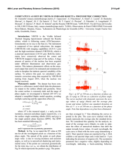
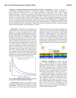
© Copyright 2026