1. Art and Diseño

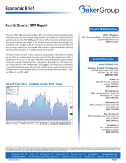
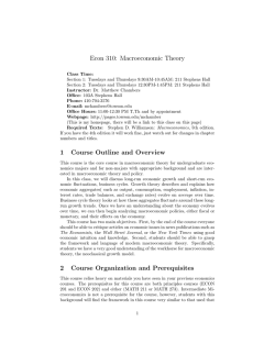
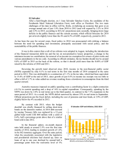
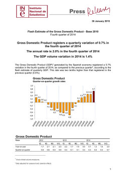
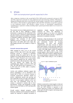
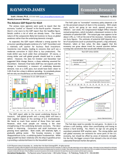
Discussion Paper
Deutsche Bundesbank
No 46/2014
Banking market structure and
macroeconomic stability:
are low-income countries special?
Franziska Bremus
(German Institute for Economic Research (DIW Berlin))
Claudia M. Buch
(Deutsche Bundesbank)
Discussion Papers represent the authors‘ personal opinions and do not
necessarily reflect the views of the Deutsche Bundesbank or its staff.
Editorial Board:
Daniel Foos
Thomas Kick
Jochen Mankart
Christoph Memmel
Panagiota Tzamourani
Deutsche Bundesbank, Wilhelm-Epstein-Straße 14, 60431 Frankfurt am Main,
Postfach 10 06 02, 60006 Frankfurt am Main
Tel +49 69 9566-0
Please address all orders in writing to: Deutsche Bundesbank,
Press and Public Relations Division, at the above address or via fax +49 69 9566-3077
Internet http://www.bundesbank.de
Reproduction permitted only if source is stated.
ISBN 978–3–95729–112–7 (Printversion)
ISBN 978–3–95729–113–4 (Internetversion)
Non-technical summary
Research Question
The structure of banking markets in low-income countries differs from that in higher-income
economies. Banking systems in low-income countries are typically smaller and less open.
Consequently, access to finance is more limited. Moreover, the effects of volatility on growth
and welfare are more pronounced. One reason for differences in macroeconomic stability
between low- and higher-income economies could be differences in the structure of banking
markets.
Contribution
In this paper, we investigate whether banking market structures affect macroeconomic
volatility and whether this link differs in low-income countries. Based on micro- and macrolevel data, we explore the channels through which the structure of banking markets impacts
macroeconomic stability. A special focus lies on low-income countries. Using a panel-dataset
that covers the period 1997-2011 and 89 countries, of which 13 are classified as “lowincome” economies, we analyze the role of banking sector risk, banking sector size, and
financial openness for the volatility of GDP per capita growth.
Results
The regression results reveal that bank-level risk as measured by bank-specific volatility can
have an impact on macroeconomic volatility. Countries with more risky or more volatile
banking systems tend to experience higher macroeconomic volatility in the longer term.
Moreover, the larger a country’s banking system is in terms of the ratio of credit to GDP, the
stronger are macroeconomic fluctuations in the short run. The impact of international
financial integration is mixed. We find that a higher degree of cross-border asset holdings can
increase GDP-volatility in low-income countries. Yet, reducing capital controls, and hence a
higher degree of de jure financial openness, enhances macroeconomic stability.
Nicht-technische Zusammenfassung
Fragestellung
Die Struktur des Bankensektors ist in Entwicklungsländern anders als in Industrie- und
Schwellenländern. So ist das Bankensystem in Entwicklungsländern typischerweise kleiner
und weniger stark international vernetzt. Folglich ist der Zugang zu Finanzierungsquellen
begrenzter. Außerdem sind die negativen Auswirkungen gesamtwirtschaftlicher
Schwankungen auf Wachstum und Wohlstand ausgeprägter. Ein Grund für die Unterschiede
zwischen Entwicklungsländern und fortgeschrittenen Volkswirtschaften mit Blick auf die
gesamtwirtschaftliche Volatilität könnten unterschiedliche Marktstrukturen im Bankensektor
sein.
Beitrag
Das vorliegende Diskussionspapier untersucht, ob die Struktur des Bankensektors eine Rolle
für die gesamtwirtschaftliche Stabilität spielt und ob sich dieser Zusammenhang in
Entwicklungsländern und fortgeschrittenen Volkswirtschaften unterschiedlich darstellt. Wir
analysieren verschiedene Wirkungskanäle, über die sich Marktstrukturen im Bankensektor
auf die gesamtwirtschaftliche Stabilität auswirken können. Der Fokus liegt dabei auf
Entwicklungsländern. Anhand von mikro- und makroökonomischen Daten für den Zeitraum
1997-2011 und 89 Länder, unter denen 13 als Entwicklungsländer klassifiziert werden,
untersuchen wir, welche Rolle Risiko, Größe und Offenheitsgrad des Bankensystems für die
Volatilität des Pro-Kopf-Wachstums einer Volkswirtschaft spielen.
Ergebnisse
Die Regressionsergebnisse zeigen, dass bankspezifisches Risiko die gesamtwirtschaftliche
Volatilität beeinflussen kann. In Ländern mit einem risikoreicheren Bankensektor ist die
gesamtwirtschaftliche Volatilität langfristig tendenziell höher. Außerdem zeigt sich, dass die
Größe von Bankensystemen – gemessen am Verhältnis von Kreditvolumen zu
Bruttoinlandsprodukt – die Stabilität der Gesamtwirtschaft in der kurzen Frist beeinträchtigen
kann. Die Auswirkungen der internationalen Finanzmarktoffenheit sind gemischt. Wir finden,
dass ein höherer Bestand an grenzüberschreitenden Aktiva die gesamtwirtschaftliche
Volatilität in Entwicklungsländern erhöht. Eine Verringerung von Kapitalverkehrskontrollen
kann die makroökonomische Stabilität allerdings fördern.
BUNDESBANK DISCUSSION PAPER NO 46/2014
Banking Market Structure and Macroeconomic Stability: Are
Low-Income Countries Special?1
Franziska Bremus
Claudia M. Buch
DIW Berlin
Deutsche Bundesbank
Abstract
Does the structure of banking markets affect macroeconomic volatility and, if yes, is this link different
in low-income countries? Banking markets in low-income countries differ from those in developed
market economies. Banking systems in lower-income countries are typically smaller and less open. In
this paper, we explore the channels through which the structure of banking markets affects
macroeconomic volatility. Our research has three main findings. First, we study the relevance of
granular effects: if the degree of market concentration in the banking sector is sufficiently high,
idiosyncratic volatility at the bank-level can impact aggregate volatility. We find weak evidence for a
link between granular banking sector volatility and macroeconomic fluctuations. Second, a higher
share of domestic credit to GDP coincides with higher volatility in the short run. Third, a higher level
of cross-border asset holdings, i.e. a higher degree of de facto financial integration, increases volatility
in low-income countries.
Keywords: bank market structure, financial integration, granularity, macroeconomic volatility, lowincome countries
JEL-Classification: G21, E32
1
Contact address: Franziska Bremus, German Institute for Economic Research (DIW Berlin), Mohrenstraße 58,
10117 Berlin, Germany. Phone: +49 30 89789590. E-Mail: [email protected]. Discussion Papers represent the
authors' personal opinions and do not necessarily reflect the views of the Deutsche Bundesbank or its staff. This
paper is part of a research project on macroeconomic policy in low-income countries supported by the U.K.’s
Department for International Development (DFID). Franziska Bremus acknowledges funding from the DFID.
The paper was presented at the Conference on “Macroeconomic Challenges Facing Low-Income Countries:
New Perspectives” (Washington, DC, January 30–31, 2014). The views expressed herein are those of the
authors and should not be attributed to the IMF, its Executive Board, or its management, to DFID, or to the
Deutsche Bundesbank. We thank two anonymous referees, César Calderón, Atilim Seymen and the conference
participants for helpful comments and suggestions. Hanna Schwank provided very valuable research assistance.
All remaining errors or inconsistencies are our own.
1 Motivation
Negative effects of macroeconomic volatility on growth and welfare can be particularly
pronounced in low-income countries (Calderon and Yeyati 2009, Loayza et al. 2007, Pallage
and Robe 2003). Shocks are more frequent and larger. Moreover, structural characteristics of
low-income economies like a low degree of diversification can amplify the effect of shocks
(Acemoglu and Zilibotti 1997, Koren and Tenreyro 2007, 2013). Given that real and financial
cycles are closely related (Claessens et al. 2011, 2012), an additional reason for differences
between high- and low-income countries in terms of macroeconomic stability could be
differences in the structure of banking systems. The banking systems in low-income countries
in fact differ in numerous aspects from those in higher-income economies. Banking systems
in low-income countries are typically smaller and less open than those in developed
economies. Access to finance is thus more limited.
In this paper, we explore the channels through which the structure of banking markets affects
macroeconomic instability as measured by the volatility of GDP per capita.2 We particularly
focus on low-income countries. We use a linked micro-macro panel-dataset including low-,
middle-, and high-income countries. Bank-level data are taken from Bankscope. We
investigate the impact of three structural characteristics of banking systems. First, we link
annual GDP-volatility to microeconomic risk at the bank-level by drawing on the concept of
granularity (Gabaix 2011). Second, we evaluate how the size of the banking sector impacts
macroeconomic instability. Third, we analyze the effect of the degree of financial openness
on aggregate volatility.
Recent research shows how heterogeneous size distributions of firms can affect
macroeconomic volatility (Gabaix 2011). If firm sizes follow a fat-tailed power law
distribution so that market concentration is high, shocks to large firms (or banks) do not
cancel out across a large number of firms as they would under normally distributed firm
sizes. In this case, macroeconomic volatility is proportional to the product of firm-specific
volatility and the Herfindahl index of concentration – “granular volatility”. The link between
asset growth fluctuations at the bank-level and aggregate fluctuations gets stronger as market
2
Instability refers to higher volatility here. Other reasons for macroeconomic instability are not analyzed in this
paper.
1
concentration and/or idiosyncratic bank-level volatility increase – even when abstracting
from the issue of interconnectedness between large banks. Using matched bank-firm loan
data for Japan, Amiti and Weinstein (2013) find that idiosyncratic loan growth shocks at the
bank-level can explain about 40 percent of the variation in aggregate credit and investment
growth. Based on industry-level data, Carvalho and Gabaix (2013) show that part of the
recent increase in macroeconomic volatility can be attributed to the raising importance of the
financial industry.
A priori, the link between bank-specific and macroeconomic fluctuations should be stronger
if the banking sector is more concentrated. Even though banking market concentration is high
in both low- and higher-income countries (Figure 1), our results in this paper show that it is
difficult to relate macroeconomic volatility to fluctuations at the bank-level. The relation
between macroeconomic volatility and “banking granular volatility” – a weighted sum of
bank-specific asset growth volatility where each bank’s weight is given by its squared market
share – is mostly insignificant. Yet, as opposed to the link between volatilities at the microand macroeconomic level, the relationship between bank-specific credit growth shocks and
aggregate growth has been shown to be positive and significant in previous work (Amiti and
Weinstein 2013, Bremus et al. 2013, Buch and Neugebauer 2011).
While low-income countries do not necessarily have a more concentrated banking market
structure, banking sector size as measured by domestic credit to GDP is much smaller in lowthan in high-income countries (Figure 1).
The expected impact of credit to GDP on
macroeconomic volatility is not clear a priori: In the literature, credit to GDP is often used as
a proxy for financial development. Our results show a consistently positive effect of credit to
GDP on macroeconomic volatility in the short run though. This hints at the destabilizing
effects of high leverage in an economy; higher credit implies larger multiplier effects and
hence higher volatility for a given shock. Yet, in the long run, we find that a higher level of
credit to GDP can reduce volatility.
The effect of financial openness on macroeconomic stability is a priori unclear. On the one
hand, a low degree of financial openness in low-income countries (Figure 1) may shield these
economies from shocks originating abroad. Moreover, capital inflows are pro-cyclical and
volatile in low-income economies (Lane 2014). While low-income economies tend to borrow
in good times, they face credit constraints in bad times (Gavin and Perotti 1997), meaning
that they have to pay back their debt in times of unfavorable economic conditions. This can
prevent countercyclical fiscal policies and exacerbate macroeconomic volatility (Kaminsky et
2
al. 2005). On the other hand, countries which are less open financially may experience higher
macroeconomic volatility because of less international risk-sharing. Recent studies indeed
find little consistent evidence on the link between output volatility and financial openness
(Kose et al. 2003, 2009). This could be due to threshold effects (Kose et al. 2011): at low
levels of institutional or financial development, financial integration may increase volatility
on financial markets. At high levels of institutional development, financial integration would
lead to stronger fluctuations.
Figure 1: Banking Market Structures
Herfindahl index (assets)
.1
.2
.4
.15
.6
.2
.8
.25
.3
1 1.2
Domestic credit / GDP
1995
2000
years
2005
Low
2010
1995
2000
Middle
2005
Low
High
2010
Middle
High
(Foreign assets + liabilities)/GDP
De jure openness
0
.5
1
1.5
2
1 1.5 2 2.5 3 3.5
years
1995
2000
years
Low
2005
2010
1995
Middle
2000
years
Low
High
2005
2010
Middle
High
The two graphs at the top show the evolution of banking sector size and concentration by income groups. The
graphs give the median values for each income group. The two graphs at the bottom show the evolution of total
foreign assets and liabilities relative to GDP (median for each income group) and a de jure measure of financial
openness, the Chinn-Ito index of capital controls (mean for each income group).
Table 1 illustrates institutional and regulatory differences between the financial systems in
low- versus higher-income countries (i.e. middle- and high-income economies). Regarding
institutional development, the quality and range of available information about borrowers is
much lower in low-income countries. The “depth of credit information index” from the
World Bank’s Doing Business Indicators reflects the scope and accessibility of credit
information available from public or private credit registries. It ranges from 0 to 6 with higher
3
values indicating a better availability of credit information. In low-income countries, this
index is just half as high as in higher-income economies with an average of 2.15. The
differences in the coverage of private credit registries is particularly pronounced: While, on
average, 36.6 percent of the adult population are covered by private credit registries in
higher-income economies, this figure is much lower (2.5 percent) in low-income countries.
As a consequence, information asymmetries between banks and borrowers are more
pronounced. This can translate into less efficient and more risky lending in low-income
countries – both for domestic and foreign banks. In addition, deposit insurance schemes are
much less common in these countries than in higher-income economies (Barth et al. 2013).
This can cause financial instability due to bank runs, and, in turn, increase macroeconomic
volatility.
Table 1: Indicators of Institutional Development in the Banking Sector
Low-income countries
Higher-income countries
Obs
Mean
SD
Min
Max
Obs
Mean
SD
Min
Max
Depth of credit information
72
2.15
1.85
0
6
454
4.47
1.44
0
6
Public registry coverage (% of adults)
Private registry coverage (% of
adults)
Deposit insurance funds relative to
total bank asset
Percent of 10 biggest banks rated
by international rating agencies
72
3.56
6.45
0
26.4
454
8.47
16.84
0
100
72
2.48
7.63
0
33.9
454
36.56 35.27
0
100
29
11.4
19.5
0
57.2
380
35.25 28.31
0
100
48
22.1
38.9
0
100
714
69.04 32.54
0
100
66
0.39
0.22
0.06
0.84
732
0.35
0.30
0
1
66
0.15
0.19
0
0.70
750
0.16
0.20
0
0.80
Share of foreign-owned banks
Share of total bank assets that are
government-owned
These descriptive statistics are based on the baseline regression sample (Table 3, column 1). The index of the
depth of credit information, as well as public and private registry coverage are available from the Doing
Business Indicators by the World Bank. The remaining information is taken from Barth et al. (2013). Definitions
and sources of each indicator can be found in the Appendix. Higher-income economies include middle- and
high-income countries.
In terms of the effects of financial openness on macroeconomic volatility, we find differences
according to the measure of financial openness used. Higher de jure openness in the sense of
weaker controls on cross-border capital flows has a stabilizing effect. Higher de facto
openness measured through foreign assets and liabilities relative to GDP, has a volatilityenhancing effect in low-income countries. These differences point to the importance of
managing international financial integration and strengthening institutions when opening up
for foreign capital.
In the following Part 2, we describe our data. Part 3 presents the regression model and the
results, while Part 4 concludes.
4
2 Data and Measurement of Volatility
2.1
Macroeconomic and Bank-Level Data
The macroeconomic data used in this paper are taken from the World Development
Indicators (WDI) by the World Bank. Details on the measurement and the data sources are
given in the Appendix; Table 2 shows descriptive statistics for the baseline regression
sample.
We start from a dataset which includes a large variety of countries, and we keep those with
complete strings of observations of at least ten years for key variables, including GDP per
capita growth and domestic credit relative to GDP. This sample includes 89 countries for 15
years (1997-2011). Due to the unbalanced nature of the panel, the maximum number of
country-year observations is 1106 if we include control variables.
Our country sample includes 13 low-income countries. We define the group of low-income
economies following the classification of the Poverty Reduction and Growth Trust (PRGT)eligible countries from the IMF. In our sample, these are Bangladesh, Bolivia, Cote d’Ivoire,
Kenya, Kyrgyz Republic, Malawi, Moldova, Mongolia, Nepal, Tanzania, Uganda, Vietnam,
and Zambia. In terms of macroeconomic data, we could use a larger country sample, but the
binding constraint is finding low-income countries with a sufficiently large number of banks.
We keep only those countries which contribute at least two observations to the baseline
regressions.
Our source for bank-level data is Bankscope, a commercial database provided by Bureau van
Dijck which provides income statements and balance sheets for banks worldwide. In
Bankscope, we have banking data for more than these 13 low-income countries, but the
number of banks for many of the low-income countries is less than five per year.
A number of screens are imposed on the banking data in order to eliminate errors due to
misreporting. We exclude the bottom 1% of the observations for total assets, and we drop
observations where the loans-to-assets or the equity-to-assets ratio is larger than one. We also
drop banks with negative equity, assets, or loans. This reduces the sample size by about 5%.
5
Table 2: Descriptive Statistics
These descriptive statistics are based on the baseline regression sample (Table 3, column 1).
Full Sample
Macroeconomic volatility
GDP per capita growth (squared residuals)
Banking sector structure
Domestic credit to the private sector / GDP
HHI (assets)
Market capitalization of listed companies / GDP
Banking granular volatility (assets)
Banking granular volatility (assets, time-invariant variance)
Mean banking sector risk (assets)
Mean banking sector risk (assets, time-invariant variance)
Macroeconomic control variables
Real private consumption per capita (USD)
Inflation (consumer prices, annual)
(Exports + Imports) / GDP
Volatility of Terms of Trade (absolute residuals)
M2 / GDP
Volatility of M2 / GDP (absolute residuals)
Government final consumption expenditure / GDP
Share of government-owned banks
Banking sector openness
(Total foreign assets + liabilities) / GDP
Chinn-Ito index of capital controls
Low-income countries
Macroeconomic volatility
GDP per capita growth (squared residuals)
Banking sector structure
Domestic credit to the private sector / GDP
HHI (assets)
Market capitalization of listed companies / GDP
Banking granular volatility (assets)
Banking granular volatility (assets, time-invariant variance)
Mean banking sector risk (assets)
Mean banking sector risk (assets, time-invariant variance)
Macroeconomic control variables
Real private consumption per capita (USD)
Inflation (consumer prices)
(Exports + Imports) / GDP
Volatility of Terms of Trade (absolute residuals)
M2 / GDP
Volatility of M2 / GDP (absolute residuals)
Government final consumption expenditure / GDP
Share of Government-owned banks
Banking sector openness
(Total foreign assets + liabilities) / GDP
Chinn-Ito index of capital controls
6
Obs.
Mean
Std. Dev.
Min.
Max.
1106
0.02
0.02
0.00
0.19
1106
1106
1106
1106
1106
1106
1106
0.72
0.24
0.54
0.05
0.08
0.02
0.04
0.55
0.18
0.66
0.04
0.05
0.03
0.03
0.02
0.01
0.00
0.00
0.02
0.00
0.00
2.84
1.00
6.06
0.47
0.40
0.33
0.21
1106 7537.45 8132.34 184.26 32011.91
1106 0.07
0.33
-0.04
10.58
1106 0.91
0.61
0.16
4.46
982
0.05
0.05
0.00
0.36
1106 0.78
0.55
0.09
3.28
1106 0.04
0.04
0.00
0.28
1106 0.16
0.05
0.05
0.30
816
0.16
0.20
0.00
0.80
1106
1106
2.83
1.00
3.83
1.52
0.38
-1.86
33.34
2.44
Obs.
Mean
Std. Dev.
Min.
Max.
130
0.02
0.02
0.00
0.11
130
130
130
130
130
130
130
0.29
0.23
0.14
0.05
0.08
0.02
0.03
0.23
0.17
0.12
0.04
0.04
0.03
0.02
0.04
0.07
0.00
0.00
0.04
0.00
0.01
1.25
1.00
0.51
0.33
0.21
0.19
0.09
130 448.81
130 0.09
130 0.73
128 0.06
130 0.41
130 0.03
130 0.12
66
0.15
130
130
1.23
0.27
214.38
0.07
0.33
0.06
0.23
0.03
0.05
0.19
0.65
1.45
184.26 1108.32
-0.00
0.39
0.32
1.78
0.00
0.27
0.11
1.25
0.00
0.19
0.05
0.21
0.00
0.70
0.42
-1.86
3.47
2.44
In order to eliminate large (absolute) growth rates that might be due to bank mergers, we
winsorize growth rates at the top or bottom percentile, i.e. the growth rates are replaced with
the respective percentiles. In terms of specializations of banks, we keep bank holding
companies, commercial banks, cooperative banks, and savings banks.3
2.2
Measuring Macroeconomic Volatility
The dependent variable of interest is the volatility of GDP per capita growth. Many previous
studies use the standard deviation of GDP growth rates as a measure of (aggregate) volatility,
where the standard deviation is calculated over a certain window of observations of five or
ten years. The disadvantage of this method is that the choice of the time window is somewhat
arbitrary and, perhaps more importantly, that the dependent variable is autocorrelated by
construction. This autocorrelation needs to be taken into account when estimating the
determinants of volatility by, for instance, estimating a dynamic panel model. Yet, dynamic
panel models are sensitive to the choice of the instruments.
For these reasons, we resort to a simple alternative measure of volatility, which has been used
in recent work by Kalemli-Ozcan et al. (2010), Loutskina and Strahan (2014) or Morgan,
Rime and Strahan (2004). To calculate the volatility of house prices, Loutskina and Strahan
(2014) use the absolute deviation of house price growth after removing time and regional
fixed effects. Applying their methodology, we regress the growth of GDP per capita on
country-fixed effects and time-fixed effects
ln GDP , ‐ ln GDP
where
and
,‐
Δ ln GDP ,
α
γ
GDPShock
,
(1)
are time- and country-fixed effects, respectively. The residual of this
regression informs us about how much GDP per capita growth in country c differs from the
average GDP-growth rate in this year across all countries and from average growth of country
c. The absolute value of this growth shock captures GDP-growth fluctuations in each country
and year. The volatility of GDP growth is thus given by
,
, . In
order to prevent large outliers from affecting the results, large growth rates in the top and
bottom percentile are winsorized. This measure of volatility can be interpreted as the annual
3
In low-income countries, public banks may play a different role for macroeconomic stability than in advanced
economies. The Bankscope data used in our regressions include information on partially publicly-owned banks.
Yet, analyzing the effects of bank-level volatility separately for private and public banks is not feasible because
we do not have consistent ownership data for all banks.
7
equivalent to the standard deviation of GDP-growth of each country across time. Figure 2
shows that macroeconomic volatility, measured by absolute residuals, has increased across all
income groups during the global financial crisis and has subsequently fallen.
Figure 2: Aggregate and Idiosyncratic Volatility
.01
.02
.03
.04
Volatility of GDP / capita (absolute residuals)
1995
2000
years
Low
High
2010
Middle
Banking granular volatility (assets)
Banking granular volatility (loans)
0
0
.02
.02
.04
.04
.06
.06
.08
.1
.08
2005
1995
2000
years
2005
2010
1995
Low
High
2000
years
2005
2010
Middle
This figure plots the volatility of growth in real GDP per capita and idiosyncratic volatility in the banking sector.
All graphs give the median values for different income groups. “absolute residuals” are the absolute values of
residuals of a regression of GDP per capita growth rates on time and country fixed effects. Banking granular
volatility is computed as described in the main body of the text, using idiosyncratic asset (loan) volatility and
squared market shares of each bank. Asset (loan) volatility is computed as the squared absolute value of
residuals of a regression of bank-level asset (loan) growth on a set of country-and-year-fixed effects.
8
2.3
Banking Granular Volatility
In addition, we need a measure of the volatility at the bank-level. Using a discrete choice
model with heterogeneous banks, Bremus et al. (2013) theoretically show that bank-specific
assets growth shocks can translate into fluctuations of aggregate credit in highly concentrated
markets, and hence into aggregate investment and output fluctuations. To compute banking
granular volatility (BGV), i.e. the weighted sum of idiosyncratic asset growth volatility at the
bank-level in each country and year, we proceed in two steps. Let
be bank i’s assets (or
,
loans) at time t where bank i is located in country c. In a first step, we regress the growth of
bank assets on fixed effects, and we retain the residuals:
ln
where
,
ln
,
Δ ln
,
,
,
is a set of country-and-year fixed effects4 and Δ ln
,
,
(2)
is the log growth rate of
bank i’s assets. The residual of equation (2) is a measure for idiosyncratic shocks at the banklevel, which is purged from macroeconomic and common banking factors.
In a second step, we compute banking granular volatility following Gabaix (2011) and
Carvalho and Gabaix (2013). These authors show that, if granularity holds, macroeconomic
volatility is proportional to the product of firm-level volatility and market concentration:
/
where
represents firm i’s sales and
is the variance of sales at the firm-level,
is
total output at time t. Applying this concept to the banking sector, we calculate BGV based
on the squared absolute values of the resulting residual growth rate of bank assets from
equation (2). This gives the variance of idiosyncratic asset growth. To check the robustness of
our results, we also use loans.
We then multiply this residual volatility with the squared market share of each bank i, and we
sum across all banks per country and year. Hence, we construct a weighted measure of
idiosyncratic volatility at the bank-level:
/
,
∑
,
∙
,
,
(3)
4
This set of fixed effects includes country fixed effects, year fixed effects and the interactions between country
and year fixed effects.
9
where
denotes total assets of bank i in country c at time t, whereas
,
,
are aggregate
total bank assets in country c and year t.
Figure 2 shows that aggregate and bank-level volatility have different time patterns.
Aggregate volatility has shown distinct time trends – a “Great Moderation” before the crisis,
followed by a spike in volatility at the time of crisis. Bank-level volatility has, if anything,
tended to decline over time. In terms of differences across countries, banking granular
volatility – be it based on loans or on total assets – was higher in low-income countries than
in high-income countries.
To interpret our results, it is useful to decompose banking granular volatility into different
components.5 In order to simplify notation, we rewrite BGV as
,
where
is bank-specific volatility and
,
,
,
,
is the squared market share of bank i
in country c at time t. Following Di Giovanni et al. (2012), BGV can be split up in the
following way:
ε, ∑ s
BGV ,
where ∑
∑
,
,
2s̅
,
,
∑ s ε
,
∑ s
,
‐s̅
∑ s
,
‐s̅
,
‐ε
,
‐const
(4)
is the Herfindahl index in country c’s banking sector at time t and
country c’s banking sector. The weights for bank risk
,
ε
reflects mean risk, i.e. the weighted average risk - as measured by volatility - of
,
share
,
,
are given by each bank’s market
.
,
ε
,
‐ε
,
is the “curvature”, that is the interaction between the Herfindahl
index of concentration and mean risk of the banking sector, where ε , denotes the average
variance of banks’ asset growth in country c at time t, s̅
on banks’ assets, and
,
is the average market share based
is a constant. A detailed derivation of this decomposition can be
found in the Appendix.
The curvature term has a very intuitive interpretation: If the curvature is positive, the banks
with the largest market shares,
5
,
, in country c’s banking sector are risky banks in the sense
We owe this point to our discussant César Calderón.
10
that they are more volatile than the average, ̅ , . If the curvature is negative, the largest banks
in country c are safer than average, i.e. volatility
,
of the most important banks is smaller
than ̅ , .
Figure 3 shows the median values for the three main components of banking granular
volatility (BGV). The top panel plots the medians of concentration, mean risk, and curvature
for the full sample, together with the 25-, 50-, and 75-% quantiles of BGV. In the full sample,
concentration is the most important part of BGV, followed by mean risk. Curvature is
negative across all quantiles. That is, BGV is mostly driven by high concentration and mean
risk, while the largest banks are, on average, less volatile than the average. This reduces the
size of banking granular volatility and hence the role of the banking system as a potential
source of aggregate volatility.
The bottom panel of Figure 3 divides the sample by income groups. The average riskiness of
the banking sector is the dominant component of banking sector volatility in low-income
countries. Also, the curvature term is only slightly negative, which means that the banks with
the largest market shares are relatively risky. For middle-income countries, the curvature term
is well below zero, indicating that the largest banks are safer than the average and reduce
banking granular volatility. Mean risk is less important but concentration is more important in
middle-income countries compared to low-income economies. Patterns are similar for highincome economies.
Decomposing banking granular volatility into its three main parts thus reveals that more
concentrated banking systems need not be necessarily the riskier ones. If banks with the
largest market shares are rather safe (less volatile than the average bank in the market), then
BGV can be low even if concentration is high. However, if the big banks are the risky ones in
the market, the curvature term of BGV can be positive. As a consequence, BGV is elevated
due to the compounding effect of concentration and high riskiness of the largest players in the
market. Given that the risk structure of banking sectors differs across countries, the
decomposition of BGV illustrates that banking systems with the same degree of concentration
can have different mean risk.
11
Figure 3: Decomposing Banking Granular Volatility (BGV)
BGV by quantile
.1
.05
0
.05
Concentration
Curvature
-.05
-.05
0
-.05
0
.05
.1
.05
0
-.05
75%-quantile
50%-quantile
.1
25%-quantile
.1
Full sample
Mean risk
BGV by income group
.05
-.05
0
-.05
0
.05
.1
0
-.05
.05
0
Concentration
Curvature
High inc
.1
Middle inc
.1
Low inc
-.05
.05
.1
Full sample
Mean risk
This figure shows the decomposition of BGV based on total assets as laid out in equation (4) in the text. The
first panel shows the median values for concentration, mean risk and curvature for the full sample and the three
quartiles. The second panel plots the median values for the full sample and for each income group. Note that the
“curvature” component is negative if larger banks are less volatile than the average. This reduces overall
banking sector volatility.
12
2.4
Banking Sector Size and Concentration
We measure the size of banking markets as the share of domestic credit to the private sector,
relative to GDP. Even though credit to GDP has increased in low-income countries during the
last years, it remains much lower than in advanced economies (Figure 1). Previous literature
has often interpreted the share of credit to GDP as a measure for financial development (Beck
et al. 2000, Levine et al. 2000). Yet, credit to GDP is also a measure for the degree of
leverage in an economy.
The concentration of banking markets, i.e. the dispersion of assets across banks, is measured
through the banking system’s Herfindahl index (HHI). The underlying data are taken from
Bankscope.6 The HHI is computed as the sum of banks’ squared market shares for each
country and year. We use this measure of concentration because the effects of idiosyncratic
shocks on aggregate developments, i.e. granular effects, tend to be stronger in more
concentrated markets.
Figure 1 reveals that banking market concentration has followed a downward trend in our
sample. The Herfindahl index tends to be higher in the most developed economies, which
may point to a larger role of granular effects for macroeconomic stability for this group of
countries.
2.5
Financial Openness
To measure the degree of financial openness, we use a de facto and a de jure measure. Our de
facto measure is taken from an updated and extended version of the external wealth dataset
constructed by Lane and Milesi-Ferretti (2007), which is available for the period 1970-2011.
In the international trade literature, the degree of trade openness is often measured as the sum
of imports and exports relative to GDP. In line with this, we use the sum of foreign assets and
foreign liabilities relative to GDP as a proxy for de facto financial integration. Note that this
measure of financial integration includes not only cross-border bank lending, but also foreign
direct investment (FDI) and portfolio investment. We opt for this broad measure of financial
integration because data on external “other investment” or “bank loans” are available for a
much smaller sample of low-income countries only.
6
Note that Bankscope does not cover all banks in a given country and year. Consequently, the Herfindahl index
computed from Bankscope is a proxy for concentration.
13
Information on capital controls as a de jure measure of financial openness comes from Chinn
and Ito (2006, 2008). These authors use the IMF’s Annual Report on Exchange Restrictions
and Regulations to construct a measure of capital account openness. The Chinn-Ito index is
based on dummy variables which codify restrictions on cross-border financial transactions.
The minimum number is -1.82 (financially closed), the maximum number is 2.46 (financially
open). Hence, both financial openness measures are scaled such that a higher number
indicates a more open financial system.
The bottom panel of Figure 1 shows our measures of de facto and de jure financial openness.
Low-income countries are generally less open than high-income countries. Financial
openness in low- and middle-income countries is similar. At the beginning of the sample
period, the ratio of foreign assets and liabilities to GDP was even higher in low- than in
middle-income economies. This is due to the fact that the official sector in low-income
countries holds high amounts of foreign reserves (Lane 2014). On the liability side, official
debt dominates. This leads to a relatively high ratio of foreign assets and liabilities to GDP in
low-income countries. In terms of de jure openness, low-income countries mostly have less
open capital accounts than middle-income economies.
3 Empirical Model and Results
With data on macroeconomic volatility and bank market structures at hand, we are now in the
position to answer our main research questions: Does the structure of banking markets affect
macroeconomic volatility and, if yes, is this link different in low-income countries?
3.1
Regression Model
As a baseline setup, we regress macroeconomic volatility on banking granular volatility, on
banking sector size, and on financial market integration. Hence, we estimate the following
equation:
,
where
,
,
is GDP-volatility,
macroeconomic factors,
,
,
,
is a vector of year-fixed effects capturing global
are country-fixed effects,
14
,
is banking granular volatility,
,
is the ratio of bank credit to GDP, and FI
,
includes de facto and de jure financial
market integration.
Second, we use the mean risk and the Herfindahl index of concentration as individual
regressors instead of BGV, so that the regression model becomes
,
where
,
,
,
,
,
is mean risk computed as the weighted average of bank-level asset growth
variances, the weights being each bank’s market share as described in section 2.3.
Our empirical analysis proceeds in the following steps: Table 3 presents the results for our
baseline regressions using the annual volatility of GDP per capita growth as the dependent
variable. In Table 4, we run the regressions for different income groups separately,
differentiating between low-income countries, i.e. countries classified by the IMF as Poverty
Reduction and Growth Trust (PRGT)-eligible, middle-, and high-income countries. Table 5
shows similar regressions for the full country sample, but including interaction terms between
the explanatory variables and a dummy variable for low-income countries which equals one
if a country is PRGT-eligible. The purpose of both sets of regressions is to analyze the
determinants of macroeconomic volatility while allowing for differences between lowincome countries and the remaining sample. Table 6 presents results from cross-sectional
regressions of the baseline specification to evaluate longer-term relationships between bank
market structures and macroeconomic stability. Finally, we show selected results from
robustness tests in Tables 7 and 8.
3.2
Determinants of Macroeconomic Stability
Banking granular volatility. Banking granular volatility does not significantly impact
aggregate stability (Table 3). Presumably, this is due to the high degree of variability in the
annual BGV. Concentration as measured by the Herfindahl index does not have a significant
impact on annual macroeconomic fluctuations either. When taking longer-term averages, as
is done in Table 6, countries with higher BGV experience higher aggregate volatility.
Intuitively, higher average risk in the banking system is related to higher GDP-volatility. If
the banking system is more risky, firms’ access to finance from banks gets more volatile so
that investment and output tend to fluctuate more. Higher banking sector concentration does
not significantly affect aggregate volatility in the longer-term.
15
Table 3: Determinants of the Volatility of GDP per Capita
(1)
Banking Granular Volatility (BGV)
BGV (assets)
0.006
(0.293)
HHI (assets)
(Foreign assets + liabilities) / GDP
Chinn-Ito index of capital controls
(4)
(5)
(6)
0.010
(0.518)
-0.004
(-0.153)
-0.005
(-0.882)
-0.005
(-0.240)
-0.010
(-1.220)
0.018*** 0.018*** 0.028*** 0.028*** 0.033** 0.033**
(2.680)
(2.762)
(2.672)
(2.680) (2.466) (2.499)
-0.000
-0.000
-0.000
-0.000
0.000
0.000
(-0.897)
(-0.898)
(-0.240)
(-0.273) (0.214) (0.140)
-0.004*** -0.004*** -0.004*** -0.003*** -0.003* -0.003*
(-3.107)
(-3.130)
(-2.914)
(-2.905) (-1.858) (-1.748)
Macroeconomic control variables
Market capitalization of listed companies / GDP
Private consumption per capita
Government consumption expenditure / GDP
Inflation (consumer prices)
Money and quasi money (M2) / GDP
Absolute residual of M2 / GDP
(Imports + Exports) / GDP
Share of government-owned banks
Observations
R²
Number of countries
(3)
0.007
(0.318)
-0.002
(-0.097)
-0.006
(-0.998)
Mean risk (assets)
Banking market structure
Domestic credit to private sector / GDP
(2)
1,106
0.110
89
1,106
0.111
89
-0.003
-0.003
-0.001 -0.001
(-0.821)
(-0.820) (-0.341) (-0.360)
-0.000
-0.000
-0.000 -0.000
(-0.124)
(-0.150) (-0.876) (-0.946)
0.020
0.024
0.080
0.083
(0.308)
(0.376) (1.178) (1.276)
0.003
0.003
0.048
0.051
(1.584)
(1.609) (1.510) (1.560)
-0.023*** -0.022** -0.024* -0.023*
(-2.659)
(-2.607) (-1.961) (-1.935)
0.026
0.026
0.019
0.019
(1.251)
(1.242) (0.776) (0.756)
0.011
0.011
0.013
0.013
(1.297)
(1.319) (1.111) (1.112)
-0.015 -0.013
(-1.615) (-1.541)
1,106
1,106
816
816
0.130
0.131
0.172
0.174
89
89
85
85
The dependent variable is macroeconomic volatility measured as the absolute value of the residual of a
regression of (log) growth in real GDP per capita on time and country fixed effects. Time and country fixed
effects are included in all regressions but are not reported. ***, **, * = significant at the 1%, 5%, 10% level.
Coming back to the panel-regressions, we find that the effect of BGV on GDP-volatility is
weakly significant and negative in low-income countries (Table 4). When including
interaction terms for low-income countries (Table 5), the effects of most explanatory
variables remain the same as in the baseline setup. The direct effect of BGV remains
insignificant. The interaction term itself is negative and significant, i.e. granular effects from
banking are weaker and even negative in low-income countries. Contrary to intuition, higher
banking sector risk reduces aggregate volatility in low-income countries. In countries where
16
access to finance is limited, more risky banking systems may enhance macroeconomic
stability if they provide more financial services and hence access to finance. Considering
mean risk and concentration as separate regressors, their effects are mostly insignificant for
macroeconomic volatility in our sample of low-income countries (Tables 4 and 5).
Table 4: Determinants of GDP Volatility by Income Group
Banking Granular Volatility (BGV)
BGV (assets)
Mean risk (assets)
(1)
(2)
Low-income
-0.074*
(-2.045)
HHI (assets)
Banking market structure
Domestic credit to private sector / GDP
(Foreign assets + liabilities) / GDP
Chinn-Ito index of capital controls
Macroeconomic control variables
Market capitalization / GDP
0.056*
(2.042)
0.012**
(2.316)
-0.006
(-0.944)
-0.003
(-0.199)
Private consumption per capita
0.000
(1.399)
Government consumption expenditure / GDP 0.186***
(3.175)
Inflation (consumer prices)
-0.034
(-0.797)
Money and quasi money (M2) / GDP
-0.084**
(-2.631)
Absolute residual of M2 / GDP
-0.022
(-0.587)
(Imports + Exports) / GDP
0.044
(1.452)
Observations
130
R²
0.356
Number of countries
13
-0.095
(-1.349)
0.002
(0.150)
(3)
(4)
Middle-income
0.038
(0.716)
0.031
(0.655)
0.000
(0.022)
(5)
(6)
High-income
0.006
(0.356)
-0.015
(-0.734)
-0.010
(-1.579)
0.061** 0.052** 0.051** 0.016*
0.016*
(2.284)
(2.683)
(2.592) (1.838) (1.891)
0.013*
-0.000
-0.000
0.000
0.000
(1.896)
(-0.016) (-0.003) (0.145) (0.082)
-0.006 -0.004*** -0.004** -0.005** -0.004**
(-0.900) (-2.724) (-2.704) (-2.269) (-2.180)
-0.003
(-0.189)
0.000
(1.105)
0.189**
(2.600)
-0.036
(-0.822)
-0.085**
(-2.455)
-0.020
(-0.502)
0.044
(1.421)
130
0.346
13
0.001
(0.094)
-0.000
(-1.476)
0.058
(0.704)
0.003
(1.430)
-0.020
(-1.087)
0.062
(1.391)
0.021
(1.117)
465
0.166
36
0.001
-0.004
-0.004
(0.098) (-1.074) (-1.028)
-0.000
-0.000
-0.000
(-1.423) (-0.299) (-0.357)
0.056
-0.014
-0.008
(0.670) (-0.094) (-0.059)
0.003
0.019
0.022
(1.431) (1.161) (1.409)
-0.019 -0.022** -0.020**
(-0.982) (-2.693) (-2.552)
0.061
0.014
0.014
(1.358) (0.508) (0.504)
0.022
-0.005
-0.006
(1.148) (-0.679) (-0.682)
465
511
511
0.164
0.172
0.176
36
40
40
The dependent variable is macroeconomic volatility measured as the absolute residual of a regression of growth
in log real GDP per capita on time and country fixed effects. Time and country fixed effects are included in all
regressions but are not reported. ***, **, * = significant at the 1%, 5%, 10% level.
Banking sector size. Macroeconomic fluctuations are higher in countries with a high level of
credit to GDP and thus a large banking sector (Tables 3 and 4). If credit to GDP was an
indicator of financial development, higher credit should lead to lower macroeconomic
volatility (Aghion et al. 1999, Easterly et al. 2001). The positive coefficient instead suggests a
destabilizing effect of higher credit. Interestingly, it is the volume of credit, not of bank
17
liabilities that has a destabilizing effect. As in previous studies (Kose et al. 2003), a higher
ratio of money supply (M2) relative to GDP decreases macroeconomic volatility, and this
effect matters especially in low-income countries.
Our findings regarding the impact of credit to GDP are in line with the results by Loayza and
Ranciere (2006) who show that the link between finance and growth varies across different
time horizons. While higher credit can support growth in the long run, a larger financial
sector can exacerbate the impact of shocks in the short run. Our cross-sectional regression
results for data averaged across the entire sample period (Table 6) confirm this interpretation:
In this long-term setup, a higher ratio of credit to GDP can reduce macroeconomic volatility.
Financial openness. De jure financial openness as measured by the Chinn-Ito index of
capital controls mitigates aggregate volatility in the full sample (Table 3). Economies with
weaker regulations on cross-border capital flows are thus more stable. A high de facto degree
of financial openness, however, can become destabilizing. The volatility of GDP growth is
higher in countries with higher foreign assets and liabilities relative to GDP, but only in the
sample of low-income countries (Tables 4 and 5). High de facto openness does not
significantly affect macroeconomic stability in the richer economies. The higher sensitivity in
low-income countries with respect to increases in de facto financial openness may be due to
the fact that institutional quality is poorer (Acemoglu et al. 2003), and financial development
is lower in low-income countries (Bekaert et al. 2006, Kose et al. 2011). As a consequence,
capital is used less efficiently.
Moreover, the portfolio of foreign assets and liabilities is more tilted towards debt than
towards equity holdings in low-income countries (Lane 2014), which can harm aggregate
stability. In the longer-term, the effects of both de jure and de facto financial openness are
insignificant in the full sample (Table 6).
Economic significance. In order to gauge the economic significance of the different
explanatory variables, we compute standardized beta-coefficients. We multiply the estimated
coefficients with the standard deviation of the explanatory variable (Table 2) and divide by
the standard deviation of the dependent variable, namely the volatility of GDP per capita
growth.
18
Table 5: Determinants of GDP-Volatility with Interaction Terms
Banking Granular Volatility (BGV)
BGV (assets)
BGV (assets) * Dummy(PRGT)
Mean risk (assets)
(1)
(2)
(3)
(4)
0.017
(0.728)
-0.090**
(-2.612)
0.017
(0.720)
-0.084**
(-2.275)
0.007
(0.294)
-0.094
(-1.526)
-0.007
(-1.096)
0.019*
(1.723)
0.007
(0.285)
-0.094
(-1.460)
-0.007
(-1.185)
0.010
(0.673)
0.028**
(2.612)
0.000
(0.013)
-0.000
(-0.307)
0.003
(0.596)
-0.004***
(-2.951)
0.000
(0.015)
0.028**
(2.612)
0.017
(0.515)
-0.000
(-0.175)
0.010*
(1.742)
-0.004***
(-2.879)
-0.001
(-0.215)
0.028**
(2.628)
0.010
(0.632)
-0.000
(-0.371)
0.002
(0.431)
-0.004***
(-2.942)
-0.000
(-0.054)
0.028***
(2.635)
0.018
(0.558)
-0.000
(-0.228)
0.009
(1.396)
-0.003***
(-2.842)
-0.001
(-0.146)
-0.003
(-0.833)
-0.003
(-0.801)
0.013
(1.119)
-0.000
(-0.094)
0.000***
(2.826)
0.008
(0.110)
0.164*
(1.700)
0.003
(1.542)
-0.028
(-0.990)
-0.022**
(-2.611)
-0.044
(-1.114)
0.029
(1.284)
-0.061
(-1.297)
0.009
(1.073)
0.035
(1.253)
1,106
0.139
89
-0.003
(-0.843)
-0.003
(-0.785)
0.015
(1.268)
-0.000
(-0.131)
0.000
(1.488)
0.013
(0.170)
0.174
(1.596)
0.003
(1.563)
-0.026
(-0.853)
-0.021**
(-2.527)
-0.040
(-0.901)
0.029
(1.268)
-0.063
(-1.330)
0.009
(1.090)
0.036
(1.269)
1,106
0.139
89
Mean risk (assets) * Dummy(PRGT)
HHI (assets)
HHI (assets) * Dummy(PRGT)
Banking market structure
Domestic credit to private sector / GDP
Credit/GDP * Dummy(PRGT)
(Foreign assets + liabilities) / GDP
FI * Dummy(PRGT)
Chinn-Ito index
Chinn-Ito * Dummy(PRGT)
Macroeconomic control variables
Market capitalization of listed companies / GDP
Market capitalization * Dummy(PRGT)
Private consumption per capita
-0.000
(-0.167)
Private consumption * Dummy(PRGT)
Government consumption expenditure / GDP
0.026
(0.385)
Government consumption * Dummy(PRGT)
Inflation (consumer prices)
0.003
(1.623)
Inflation * Dummy(PRGT)
M2 / GDP
-0.023***
(-2.679)
M2 / GDP * Dummy(PRGT)
Absolute residual of M2 / GDP
0.026
(1.262)
Absolute residual of M2/GDP * Dummy(PRGT)
(Imports + Exports) / GDP
0.011
(1.326)
(Imports + Exports) / GDP * Dummy(PRGT)
Observations
R²
Number of countries
1,106
0.134
89
-0.000
(-0.244)
0.030
(0.443)
0.003
(1.644)
-0.022**
(-2.581)
0.026
(1.225)
0.011
(1.362)
1,106
0.133
89
The dependent variable is macroeconomic volatility measured as the absolute residual of a regression of growth
in log real GDP per capita on time and country fixed effects. Time and country fixed effects are included in all
regressions but are not reported.
***, **, * =
significant at the 1%, 5%, 10% level.
19
Table 6: Cross-Sectional Baseline Regressions
(1)
Banking Granular Volatility
BGV (assets)
Mean risk (assets)
HHI (assets)
0.146**
(2.540)
(2)
0.219**
(2.416)
0.009
(1.028)
Banking market structure
Domestic credit to private sector / GDP -0.009*** -0.009***
(-3.619)
(-3.697)
0.000
0.000
(Foreign assets + liabilities) / GDP
(1.349)
(1.574)
0.001
0.001
Chinn-Ito index of capital controls
(0.904)
(0.916)
Macroeconomic control variables
Market capitalization / GDP
Private consumption per capita
Government consumption expenditure /
GDP
(3)
0.145***
(2.850)
(4)
0.243***
(2.648)
0.006
(0.662)
(5)
0.181***
(3.937)
(6)
0.310***
(3.592)
0.008
(0.957)
-0.006
(-1.130)
-0.001
(-0.785)
0.001
(1.086)
-0.007
(-1.340)
-0.001
(-0.842)
0.001
(1.061)
0.002
(0.522)
-0.000
(-0.746)
0.001
(1.072)
0.001
(0.149)
-0.000
(-0.895)
0.001
(1.046)
-0.005*
(-1.857)
-0.000
(-0.006)
-0.019
-0.005*
(-1.892)
0.000
(0.023)
-0.015
-0.003
(-1.261)
-0.000
(-1.066)
0.005
-0.003
(-1.386)
-0.000
(-1.114)
0.010
(-0.514)
0.013
(0.969)
0.002
(0.264)
0.092
(1.014)
0.006
(1.612)
(-0.403)
0.008
(0.570)
0.002
(0.280)
0.115
(1.162)
0.007
(1.614)
(0.171)
(0.367)
0.014
0.007
(1.025)
(0.508)
-0.007*
-0.007
Money and quasi money (M2) / GDP
(-1.802)
(-1.653)
0.113
0.149*
Absolute residual of M2 / GDP
(1.583)
(1.900)
0.007**
0.007**
(Imports + Exports) / GDP
(2.235)
(2.441)
0.009
0.009
Share of government-owned banks
(1.203)
(1.129)
89
89
89
89
85
85
Observations
0.142
0.144
0.237
0.244
0.315
0.334
R²
The dependent variable is macroeconomic volatility measured as the average of year-on-year GDP-volatility
across the sample period (1997-2011). ***, **, * = significant at the 1%, 5%, 10% level.
Inflation (consumer prices)
An increase in BGV by one standard deviation implies an increase of 0.01 standard
deviations in macroeconomic volatility in the full sample. De jure financial openness and
credit to GDP are economically much more important with standardized beta-coefficients of 0.3 and 0.8, respectively. For the sub-sample of low-income countries, the ranking is the
same as in the full sample: credit to GDP matters most for macroeconomic volatility,
followed by de facto financial openness. Banking granular volatility is economically much
less important.
20
However, an increase in financial openness and credit to GDP leads to higher macroeconomic
volatility in low- than in high-income countries. When estimating the model separately by
income group (Table 4), credit to GDP has a higher economic significance for the lowincome than for the high-income countries: The standardized beta-coefficients reveal that an
increase in credit to GDP by one standard deviation increases macroeconomic volatility by
0.7 standard deviations in low-income countries. In high-income economies, a one standard
deviation increase in credit to GDP raises macroeconomic volatility by 0.45 standard
deviations only. Again, weaker institutions in low-income countries may explain the
difference. In the cross-sectional regressions, the economic significance of BGV is as high as
the economic significance of credit to GDP with a standardized beta coefficient of 0.3.
3.3
Robustness Tests
In order to test the robustness of our results, we have run several alternative regressions. First,
we have used banking granular volatility and its components based on loans instead of assets
as an alternative specification of banking sector volatility.7 The results remain broadly the
same. Moreover, following Carvalho and Gabaix (2013), we have computed BGV using
(time-invariant) standard deviations for each bank across the sample period instead of the
time-varying squared absolute values of bank-specific shocks. This allows us to concentrate
on the effects of market structure by abstracting from changes in annual bank-specific
volatilities. Table 7 reveals that this alternative measure of granular effects from the banking
sector does not affect the results for the full sample. In the sample of low-income countries,
the negative effect of BGV turns insignificant if BGV is based on time-invariant volatility
(not reported).
Second, in order to test how our results are influenced by the global financial crisis, we
interact all variables of interest with a banking-crisis dummy which is available from Laeven
and Valencia (2012). Again, the results remain broadly unchanged. The effect of the
Herfindahl index on GDP-volatility turns negative when including an interaction with the
crisis-dummy. As expected, volatility is higher in times of crisis. Hence, higher banking
sector concentration increases volatility in crisis times while it stabilizes output in normal
times.
7
The regression results are available upon request.
21
Table 7: Baseline Regressions with Time-Invariant Bank-Level Volatility
(1)
Banking Granular Volatility
BGV (assets, time-inv. var.)
Mean risk (assets, time-inv. var.)
HHI (assets)
Banking market structure
Domestic credit to private sector / GDP
(Foreign assets + liabilities) / GDP
Chinn-Ito index of capital controls
0.007
(0.323)
(2)
0.089
(1.655)
-0.009
(-1.309)
(3)
(4)
0.008
(0.394)
0.077
(1.556)
-0.007
(-1.188)
0.018*** 0.018*** 0.028*** 0.027***
(2.676)
(2.904)
(2.674)
(2.708)
-0.000
-0.001
-0.000
-0.000
(-0.935)
(-1.065)
(-0.266)
(-0.399)
-0.004*** -0.004*** -0.004*** -0.004***
(-3.105)
(-3.149)
(-2.904)
(-2.921)
Macroeconomic control variables
Market capitalization / GDP
Private consumption per capita
Government consumption expenditure /
GDP
-0.003
(-0.837)
-0.000
(-0.132)
0.020
-0.002
(-0.759)
-0.000
(-0.173)
0.027
(0.316)
0.003
(1.598)
-0.023***
(-2.645)
0.026
(1.274)
0.011
(1.289)
(0.445)
0.003*
(1.769)
-0.021**
(-2.560)
0.026
(1.260)
0.010
(1.225)
(5)
0.017
(0.533)
(6)
0.085
(1.174)
-0.010
(-1.375)
0.033**
(2.470)
0.000
(0.169)
-0.003*
(-1.858)
0.033**
(2.525)
0.000
(0.040)
-0.003*
(-1.861)
-0.001
(-0.358)
-0.000
(-0.842)
0.083
-0.001
(-0.310)
-0.000
(-0.963)
0.086
(1.229)
(1.335)
0.047
0.049
(1.494)
(1.501)
-0.024*
-0.021*
Money and quasi money (M2) / GDP
(-1.950)
(-1.890)
0.020
0.019
Absolute residual of M2 / GDP
(0.811)
(0.785)
0.013
0.012
(Imports + Exports) / GDP
(1.117)
(1.031)
-0.014
-0.012
Share of government-owned banks
(-1.587)
(-1.413)
1,106
1,106
1,106
1,106
816
816
Observations
0.110
0.116
0.130
0.134
0.172
0.177
R²
89
89
89
89
85
85
Number of countries
The dependent variable is macroeconomic volatility measured as the absolute residual of a regression of growth
in log real GDP per capita on time and country fixed effects. BGV is computed based on the time-invariant
variances of bank assets as described in the main body of the text. Time and country fixed effects are included in
all regressions but are not reported. ***, **, * = significant at the 1%, 5%, 10% level.
Inflation (consumer prices)
Third, we interact credit to GDP and de facto financial openness with variables measuring
institutional quality in order to account for possible threshold effects in the relation between
financial system size (both domestic and international) and macroeconomic volatility. We
measure institutional quality using different variables from the Doing Business Indicators and
from the World Bank Governance Indicators and include interaction terms in the regressions
for the full sample and for the sub-sample of low-income countries.
22
Table 8: Instrumental Variables Regressions
(1)
Banking Granular Volatility
BGV (assets)
-0.003
(-0.286)
Mean risk (assets)
HHI (assets)
Banking market structure
Domestic credit to private sector / GDP
0.010**
(2.207)
-0.000
(-0.198)
-0.000
(-0.225)
(Foreign assets + liabilities) / GDP
Chinn-Ito index of capital controls
Macroeconomic control variables
Market capitalization / GDP
(2)
-0.003
(-0.286)
-0.006
(-1.504)
0.011**
(2.519)
-0.000
(-0.564)
-0.001
(-1.104)
-0.002
-0.001
(-1.290)
(-0.951)
Private consumption per capita
0.147***
0.164***
(4.474)
(5.364)
Government consumption expenditure / GDP
0.009
0.010*
(1.532)
(1.742)
Inflation (consumer prices)
-0.000
-0.000
(-0.687)
(-0.096)
Money and quasi money (M2) / GDP
-0.009***
-0.009***
(-3.405)
(-3.624)
Absolute residual of M2 / GDP
0.046***
0.047***
(4.012)
(5.457)
(Imports + Exports) / GDP
-0.000
-0.007*
(-0.031)
(-1.974)
Observations
912
912
R²
0.045
0.051
Number of countries
85
85
p-value of Hansen j-statistic
0.583
0.351
Hansen j-statistic
21.94
34.46
The dependent variable is macroeconomic volatility measured as the absolute residual of a regression of growth
in log real GDP per capita on time and country fixed effects. Time and country fixed effects are included in all
regressions but are not reported. ***, **, * = significant at the 1%, 5%, 10% level.
The interactions between institutional quality indicators and credit to GDP or financial
openness are mostly insignificant. Exceptions are the interactions between an indicator for
government effectiveness and for the control of corruption and credit to GDP: The more
effective the government or the better the control of corruption, the weaker is the volatilityenhancing effect of credit to GDP. The remaining effects are broadly unchanged if we
include interaction terms between the size of the banking sector and institutional variables in
the full sample.
Interestingly, the effect of BGV gets more statistically significant and positive in some of the
regression models which include (insignificant) measures of institutional quality. This is due
to the different sample compositions: Most of the institutional variables are available for
23
shorter time periods or fewer countries than in our baseline sample. Hence, depending on the
sample composition, the significance of granular effects from the banking sector is more or
less pronounced.
Table 8 presents results for instrumental variables regressions. Even though BGV is
exogenous by construction, the other explanatory variables of interest may be endogenous.
For example, domestic credit may drop due to a decline in credit demand during bad times,
and financial markets may close down in periods of high macroeconomic instability.
We use the second lag of the Herfindahl index, domestic credit to GDP, and de facto and de
jure financial openness as instruments for their contemporaneous counterparts. In order to
increase efficiency of the instrumental variable regressions and to be able to run SarganHansen tests of orthogonality conditions, we employ the methodology proposed by Lewbel
(2012). This approach allows constructing heteroscedasticity-based instruments as simple
functions of the regressors. Additional external instruments can be obtained from auxiliary
(first-stage) regressions, where each endogenous variable is regressed on all exogenous
variables. The generated instruments are then obtained by multiplying the residuals from the
auxiliary regressions with the demeaned exogenous variable. Identification is achieved by
having regressors that are uncorrelated with the heteroscedastic error terms (Baum and
Schaffer 2012).
The results support our previous findings that a higher ratio of credit to GDP increases
macroeconomic volatility. When instrumenting the regressors, the effect of de jure financial
openness turns insignificant though.
4 Summary
In this paper, we study the impact of banking market structure on macroeconomic volatility
with a focus on low-income countries. Compared to higher-income countries, low-income
countries are characterized by higher average banking sector risk, lower degrees of
international integration, and smaller overall banking systems. The degree of concentration in
banking markets is similar. Our study has three main findings.
First, idiosyncratic risk at the bank-level has no strong impact on year-to-year
macroeconomic volatility. Cross-sectional regressions show that a high degree of mean risk
24
in banking markets increases aggregate volatility. Hence, we find evidence for a positive link
between bank-level and macroeconomic volatility in the longer term.
Second, a higher ratio of bank credit relative to GDP increases macroeconomic volatility,
also in low-income countries. This destabilizing effect of banking sector size occurs,
however, in the short run only. Our results point to possible volatility-reducing effects of
credit to GDP in the long run.
Third, increased financial integration is a double-edged sword. Reducing capital controls –
and thus a higher degree of de jure openness – has a stabilizing effect. High ratios of foreign
assets and liabilities relative to GDP increase macroeconomic instability in low-income
countries, in contrast.
In terms of policy implications, our results imply that there are different channels through
which macroeconomic volatility can potentially be reduced: by limiting the excessive
expansion of domestic and foreign credit in an economy, and by reducing idiosyncratic and
thus bank-level volatility. We have also shown that the impact of financial openness on
macroeconomic volatility depends on the openness measure chosen.
25
References
Acemoglu, D. and F. Zilibotti (1997) “Was Prometheus Unbound by Chance? Risk,
Diversification, and Growth,” Journal of Political Economy 105, 709-751.
Acemoglu, D., Johnson, S., Robinson, J., and Y. Thaicharoen (2003) “Institutional causes,
macroeconomic symptoms: volatility, crises and growth,” Journal of Monetary
Economics 50, 49-123.
Aghion, P., Banerjee, A., and T. Piketty (1999) “Dualism and macroeconomic volatility,”
Quarterly Journal of Economics 114, 1359-1397.
Amiti, M. and D.E. Weinstein (2013) “How much do bank shocks affect investment?
Evidence from matched bank-firm loan data,” NBER Working Paper No. 18890,
National Bureau of Economic Research, Cambridge, MA.
Barth, J. R., Caprio, G., and R. Levine (2013) “Bank Regulation and Supervision in 180
Countries from 1999 to 2011,” Journal of Financial Economic Policy 5, 111-219.
Baum, C.F. and M.E. Schaffer (2012) “IVREG2H: Stata module to perform instrumental
variables estimation using heteroskedasticity-based instruments,” Statistical Software
Components, Department of Economics, Boston College.
Beck, T., Demirgüç-Kunt, A. and R. Levine (2000) “A New Database on Financial
Development and Structure,” World Bank Economic Review 14, 597-605.
Bekaert, G., Harvey, C.R., and C. Lundblad (2006) “Growth volatility and financial
liberalization,” Journal of International Money and Finance 25, 370-403.
Bremus, F., Buch, C.M., Russ, K.N., and M. Schnitzer (2013) “Big Banks and
Macroeconomic Outcomes Theory and Cross-Country Evidence of Granularity”,
NBER Working Paper No. 19093, National Bureau of Economic Research,
Cambridge, MA.
Buch, C.M. and K. Neugebauer (2011) “Bank-specific shocks and the real economy,” Journal
of Banking and Finance 35, 2179-2187.
Calderon, C. and E.L. Yeyati (2009) “Zooming in: from aggregate volatility to income
distribution,” Policy Research Working Paper Series 4895, The World Bank,
Washington D.C.
26
Carvalho, V.M. and X. Gabaix (2013) “The Great Diversification and its Undoing,”
American Economic Review 103, 1697-1727.
Chinn, M.D. and H. Ito (2006) “What Matters for Financial Development? Capital Controls,
Institutions, and Interactions,” Journal of Development Economics 81, 163-192.
Chinn, M.D. and H. Ito (2008) “A New Measure of Financial Openness,” Journal of
Comparative Policy Analysis 10, 309-322.
Claessens, S., Kose, M.A., and M.E. Terrones (2011) “Recessions and Financial Disruptions
in Emerging Markets: A Bird’s Eye View,” in: Cespedes, L., R. Chang, and D.
Saravia (eds.) Monetary Policy Under Financial Turbulence, Central Bank of Chile.
Claessens, S., Kose, M.A., and M.E. Terrones (2012) “How do business and financial cycles
interact?” Journal of International Economics 87, 178-190.
Di Giovanni, J., Levchenko, A.A., and R. Rancière (2012) “The Risk Content of Exports: A
Portfolio View of International Trade,” NBER International Seminar on
Macroeconomics, University of Chicago Press 8, 97-151.
Easterly, W., Islam, R., and J. Stiglitz (2001) “Volatility and macroeconomic paradigms for
rich and poor countries,” in: Dreze, J. (Ed.), Advances in Macroeconomic Theory.
Palgrave, New York.
Gavin, M. and R. Perotti (1997) “Fiscal policy in Latin America,” NBER Macroeconomics
Annual 12, Cambridge, MA: MIT Press, 11-61.
Gabaix, X. (2011) “The Granular Origins of Aggregate Fluctuations,” Econometrica 79, 733772.
Kalemli-Ozcan, S., Sørensen, B.E., and V. Volosovych (2010) “Deep Financial Integration
and Volatility,” NBER Working Paper No. 15900, National Bureau of Economic
Research, Cambridge, MA.
Kaminsky, G.L., Reinhart, C.M., and C.A. Végh (2005) “When It Rains, It Pours: Procyclical
Capital Flows and Macroeconomic Policy,” in: Gertler, M., and K. Rogoff (eds.)
NBER Macroeconomics Annual 2004, Cambridge, MA: MIT Press.
Kose, M.A., Prasad, E.S., and M.E. Terrones (2003) “Financial Integration and
Macroeconomic Volatility,” IMF Working Paper No. 03/50, International Monetary
Fund, Washington, D.C.
27
Kose, M.A., Prasad, E.S., Rogoff, K., and S.-J. Wei (2009) “Financial Globalization: A
Reappraisal,” IMF Staff Papers 56, 8-62.
Kose, M.A., Prasad, E.S., and A.D. Taylor (2011) “Threshold Effects in the Process of
International Financial Integration,” Journal of International Money and Finance 30,
147-179.
Koren, M. and S. Tenreyro (2007) “Volatility and Development,” Quarterly Journal of
Economics 122, 243-287.
Koren, M. and S. Tenreyro (2013), “Technological Diversification,” American Economic
Review 103, 378-414.
Laeven, L. and F. Valencia (2012) “Systemic Banking Crises Database: An Update,” IMF
Working Paper No. 12/163, International Monetary Fund, Washington, D.C.
Lane, P.R. and G.M. Milesi-Ferretti (2007) “The External Wealth of Nations Mark II,”
Journal of International Economics 73, 223-250.
Lane, P.R. (2014) “Capital Flows in Low-Income Countries”, Paper presented at the
Conference on “Macroeconomic Challenges Facing Low-Income Countries”,
International Monetary Fund, Washington, D.C.
Levine, R., Loayza, N., and T. Beck (2000) “Financial intermediation and growth: Causality
and causes,” Journal of Monetary Economics 46, 31-77.
Lewbel, A. (2012) “Using Heteroscedasticity to Identify and Estimate Mismeasured and
Endogenous Regressor Models,” Journal of Business and Economic Statistics 30, 6780.
Loayza, N. and R. Ranciere (2006) “Financial Development, Financial Fragility, and
Growth,” Central Bank of Chile Working Papers No. 145, Central Bank of Chile.
Loayza, N.V., Rancière, R., Servén, L., and J. Ventura (2007) “Macroeconomic Volatility
and Welfare in Developing Countries: An Introduction,” World Bank Economic
Review 21, 343-357.
Loutskina, E. and P.E. Strahan (2014) “Financial Integration, Housing and Economic
Volatility,” forthcoming: Journal of Financial Economics, University of Virginia and
Boston College.
28
Morgan, D., Rime, B., and P.E. Strahan (2004) “Bank Integration and State Business
Cycles,” Quarterly Journal of Economics 119, 1555-85.
Pallage, S. and M.A. Robe (2003) “On the Welfare Cost of Economic Fluctuations in
Developing Countries”, International Economic Review 44, 677-698.
29
Appendix
1 Data Definition and Sources
Income groups: The group of low-income countries follows the classification of the Poverty
Reduction and Growth Trust (PRGT)-eligible countries from the IMF/WEO. The group of
middle-income countries includes countries which are classified as middle-income countries
by the World Bank, but without PRGT-eligible countries. High-income countries are
classified according to the World Bank.
List of countries (PRGT-eligible countries are in italics): Argentina, Armenia, Australia,
Austria, Bangladesh, Belgium, Bolivia, Botswana, Brazil, Bulgaria, Canada, Chile, China,
Colombia, Costa Rica, Cote d'Ivoire, Croatia, Cyprus, Czech Republic, Denmark, Ecuador,
Egypt, El Salvador, Estonia, Finland, France, Germany, Greece, Guatemala, Hong Kong,
Hungary, India, Indonesia, Ireland, Israel, Italy, Japan, Jordan, Kazakhstan, Kenya, Korea.
Rep., Kyrgyz Republic, Latvia, Lebanon, Lithuania, Macedonia, Malawi, Malaysia, Malta,
Mexico, Mongolia, Moldova, Morocco, Namibia, Nepal, Netherlands, New Zealand, Norway,
Pakistan, Panama, Paraguay, Peru, Philippines, Poland, Portugal, Qatar, Romania, Russian
Federation, Singapore, Slovak Republic, Slovenia, South Africa, Spain, Swaziland, Sweden,
Switzerland, Tanzania, Thailand, Trinidad and Tobago, Tunisia, Turkey, Uganda, Ukraine,
United Arab Emirates, United Kingdom, United States, Uruguay, Venezuela, Vietnam,
Zambia.
Banking granular volatility: To compute banking granular volatility as described in the text,
we use bank-level data on total net loans and total assets from the Bankscope database for the
period 1997-2011. In Bankscope, we keep observations with the consolidation codes C1
(consolidated and companion is not on the disc), C2 (consolidated and companion is on the
disc), U1 (unconsolidated and companion is not on the disc or the bank does not publish
consolidated accounts), and A1 (aggregated statements with no companion), so that doublecountings are eliminated.
Bank-level volatility: Computed as the squared absolute residual of a regression of bank-level
assets (loan) growth on country-year-fixed effects using the Bankscope dataset.
Capital controls: We use the Chinn-Ito index as a de jure measure for financial openness.
This variable measures a country’s degree of capital account openness and is available for the
period 1970-2011 and 182 countries. It ranges from -1.82 to 2.46 with a sample mean of zero.
The smaller the Chinn-Ito Index, the lower (de jure) financial openness.
Concentration: As a measure of concentration in the banking sector, we compute Herfindahlindexes for each country and year based on net loans and assets from Bankscope.
Credit to GDP: Credit to the private sector in percent of GDP is taken from the World
Development Indicators.
Deposit insurance funds relative to total bank asset: This information is available from Barth
et al. (2013).
Depth of credit information: Scope and accessibility of credit information provided by public
or private credit registries. This index ranges from 0 to 6 with higher values indicating better
availability of credit information and thus facilitated lending decisions for banks. The index is
available from the Doing Business Indicators by the World Bank.
GDP per capita growth: We compute growth as the log-difference in constant 2005 USDollars. The data on GDP per capita come from the World Development Indicators.
30
Government consumption expenditure / GDP: Data on general government final consumption
expenditure in percent of GDP (in constant 2005 USD) is taken from the World Development
Indicators.
Inflation (consumer prices, annual %): World Development Indicators.
Market capitalization of listed companies (relative to GDP): The data is taken from the World
Development Indicators.
Mean banking sector risk: We compute mean risk as the weighted sum of the squared
absolute value of idiosyncratic bank-level asset growth, where the weights are given by each
bank’s market share (see equation (4) in the main text).
M2 / GDP: Money and quasi money (M2) relative to GDP is retrieved from the World
Development Indicators.
Percent of 10 biggest banks rated by international rating agencies: This information is
available from Barth et al. (2013).
Private registry coverage (% of adults): Percentage of the adult population that is covered by
private credit bureaus. We take this information from the Doing Business Indicators by the
World Bank.
Public registry coverage (% of adults): Percentage of the adult population that is covered by
public credit registries. We take this information from the Doing Business Indicators by the
World Bank.
Real private consumption per capita (USD): Data on real private consumption and on total
population come from the World Development Indicators.
Share of foreign-owned banks: The information is available from Barth et al. (2013).
Share of total bank assets that are government-owned: The information is available from
Barth et al. (2013).
Total foreign assets and liabilities relative to GDP: We use data on total foreign assets and
liabilities in US-Dollars from the updated database by Lane and Milesi-Feretti (2007) which
is available for the period 1970-2011 for 178 countries. GDP-data is taken from the WDI.
Trade openness: We take exports and imports relative to GDP from the World Development
Indicators.
Volatility of M2 / GDP: We compute absolute residuals from a regression of M2 / GDP on
country- and time-fixed effects.
31
2 Decomposition of Banking Granular Volatility (BGV)
Following Di Giovanni et al. (2012), Banking Granular Volatility can be decomposed as
follows:
∑
∑
∑
.
Writing out the expression explicitly and simplifying, it can be shown that this decomposition
is equivalent to BGV as defined in equation (2) in the main text:
,
⇒
/
32