1. Art and Diseño

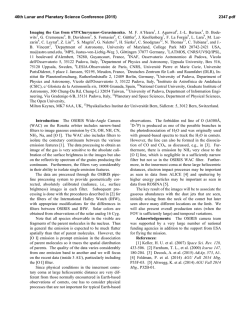
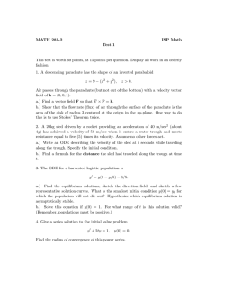
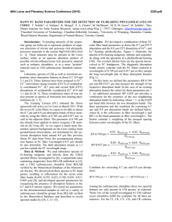
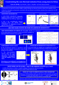
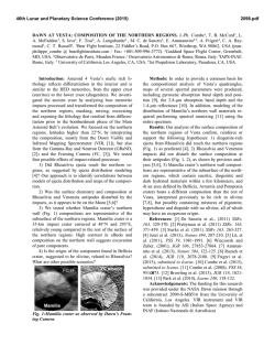
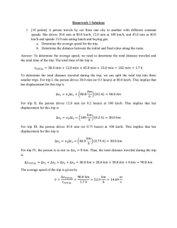
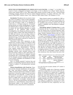
Draft version January 30, 2015
Preprint typeset using LATEX style emulateapj v. 5/2/11
A SEMI–ANALYTICAL LINE TRANSFER (SALT) MODEL TO INTERPRET THE SPECTRA OF GALAXY
OUTFLOWS
C. Scarlata1 and N. Panagia2,3,4
arXiv:1501.07282v1 [astro-ph.GA] 28 Jan 2015
Draft version January 30, 2015
ABSTRACT
We present a Semi–Analytical Line Transfer model, SALT, to study the absorption and re–emission
line profiles from expanding galactic envelopes. The envelopes are described as a superposition of
shells with density and velocity varying with the distance from the center. We adopt the Sobolev
approximation to describe the interaction between the photons escaping from each shell and the
remaining of the envelope. We include the effect of multiple scatterings within each shell, properly
accounting for the atomic structure of the scattering ions. We also account for the effect of a finite
circular aperture on actual observations. For equal geometries and density distributions, our models
reproduce the main features of the profiles generated with more complicated transfer codes. Also, our
SALT line profiles nicely reproduce the typical asymmetric resonant absorption line profiles observed
in starforming/starburst galaxies whereas these absorption profiles cannot be reproduced with thin
shells moving at a fixed outflow velocity. We show that scattered resonant emission fills in the resonant
absorption profiles, with a strength that is different for each transition. Observationally, the effect
of resonant filling depends on both the outflow geometry and the size of the outflow relative to the
spectroscopic aperture. Neglecting these effects will lead to incorrect values of gas covering fraction
and column density. When a fluorescent channel is available, the resonant profiles alone cannot be
used to infer the presence of scattered re–emission. Conversely, the presence of emission lines of
fluorescent transitions reveals that emission filling cannot be neglected.
Subject headings: galaxies: ISM — ISM: structure
1. INTRODUCTION
The mechanical and radiative energy (from massive
star winds and supernova explosions) injected in the interstellar medium (ISM) of galaxies is expected to drive
gas outflows around regions of active star–formation.
These outflows are indeed observed both on the scale
of individual H II regions as well as on full-galaxy
scales. Outflows are currently invoked as the principal mechanism regulating the galactic baryonic cycle
(i.e., the balance between the gas accretion rate and
the star-formation rate) in state-of-the-art galaxy formation models (e.g. Oppenheimer et al. 2010; Dav´e et al.
2011; Lilly et al. 2013). Whether or not the observed
outflows are actually able to do the job is, however,
still unclear. In fact, although outflow-regulated models
are able to broadly reproduce some of the fundamental
correlations observed in massive galaxies, recent studies
have pointed out the existence of a fundamental problem with the evolution of low mass (M∗ < 109.5 M⊙ )
galaxies (Weinmann et al. 2012). This difficulty appears
to indicate that crucial feedback processes are modeled
incorrectly, since it is precisely in this low-mass regime
that feedback-induced outflows are expected to have the
strongest impact.
What is lacking at this point are robust observational
1 Minnesota Institute for Astrophysics, School of Physics and
Astronomy, University of Minnesota, 316 Church str SE, Minneapolis, MN 55455,USA
2 Space Telescope Science Institute, 3700 San Martin Drive,
Baltimore, MD 21218, USA, [email protected]
3 INAF–NA, Osservatorio Astronomico di Capodimonte,
Salita Moiariello 16, 80131 Naples, Italy
4 Supernova Ltd, OYV #131, Northsound Rd., Virgin Gorda
VG1150, Virgin Islands, UK
constraints on the physical properties of galaxy outflows and how these depend on the galaxy star–formation
rates, stellar masses, and so on. In order to characterize
how effective feedback is in quenching the star–formation
(by, e.g., heating the gas and/or completely remove it
from a galaxy dark matter halo) we need to be able to
probe the kinematics of the outflows, their density structure, and their extent. Absorption line studies against
the strong UV continuum produced in the star-forming
regions can probe the neutral and ionized components of
the outflows, with numerous resonant transitions in low
and high ionization metals (such as, Si II, C II, Mg II,
C III, Fe II, andC IV; e.g., Rupke et al. 2005; Martin
2005; Sato et al. 2009; Weiner et al. 2009; Rubin et al.
2010; Steidel et al. 1996; Shapley et al. 2003).
Recent studies show that outflowing gas moving with
velocities up to several hundreds of km s−1 is common
in star–forming galaxies (e.g., Pettini et al. 2002; Martin
2005). Generally, these studies use standard absorption–
line analysis (e.g Savage & Sembach 1991), where the velocity of the outflowing material is determined by the
amount of blueshift observed in the resonant absorption
lines (typically UV lines, but absorption of Na–D lines
has been used). Recent observations, however, have revealed the presence of numerous resonant and fluorescent
emission lines associated with the blueshifted resonant
absorptions (e.g., Weiner et al. 2009; France et al. 2010;
Rubin et al. 2011; Jones et al. 2012; Erb et al. 2012;
Martin et al. 2012, 2013; Kornei et al. 2013). Although
originally interpreted as the result of photoionization by
weak AGNs (e.g., Weiner et al. 2009), these lines are now
believed to be the result of scattered resonant photons
in an expanding envelope around galaxies (Rubin et al.
2
Scarlata & Panagia
Fig. 1.— Side view of the outflow model. We consider a spherical galaxy (with radius RSF ) surrounded by an expanding envelope with
a velocity increasing radially with the distance from the center. For r > RW the gas velocity is v∞ . The shaded yellow area shows the size
of the aperture of radius Raper . The dotted vertical line indicates the edge-on view of the plane with constant observed velocity (vobs ).
2011; Erb et al. 2012; Martin et al. 2013).
The scattered re–emission into the line of sight affects
the velocity measurements based on pure absorption lines
analysis, as well as mimic a partial covering fraction of
the outflowing gas (e.g., Prochaska et al. 2011). In these
cases, it is crucial to be able to consistently model both
the resonant absorption as well as the associated resonant and (if present) fluorescent emission originating
from the same ionic species. Steps in this direction have
been taken by Rubin et al. (2011), who pioneered the
study of outflows in emission using resonantly-scattered
MgII, and Fe lines. Prochaska et al. (2011) used Monte
Carlo radiative transfer techniques to study the nature of
resonant absorption and emission for winds, accounting
for the effects of resonant scattering and fluorescence.
In this paper we go a step forward and develop a Semi–
Analytical Line Transfer (hereafter referred to as SALT)
model to interpret the absorption/scattered emission line
profiles resulting from extended galactic outflows. We
assume that the Sobolev approximation holds, and we
account for multiple scattering within the outflow with
a simple statistical approach. As an example of an application of the model, we apply SALT to multiple transitions in the Si+ ion observed in the stack spectrum of
z ∼ 0.3 Lyα emitters. We show how our model is able to
consistently reproduce the profiles of both the absorption
and resonant and fluorescent emission lines and thus constrain the outflow velocity– and density–fields. Although
rather simplified, the SALT model can be used to gain
a more physical understanding of the outflowing gas, in
both local and high redshift galaxies. We focus here on
a few specific lines of Si+ ion, however, the models are
readily applicable to any other ions.
The paper is organized as follows. In Section 2 we
present the derivation of the semi analytical line profile
for an outflowing spherical shell. The model is compared
with the observed stacked spectrum in Section 3, and the
results are discussed in Section 4. We offer our conclusions in Section 5.
2. P-CYGNI PROFILE FROM A SPHERICAL EXPANDING
ENVELOPE
In spherical outflows, such as those produced in winds
from early type stars, resonant lines are characterized
by the well understood P–Cygni profile (e.g., Castor
1970; Castor & Lamers 1979). The profile shows both
an emission and an absorption component. The absorption is created in the material between the source and
3
the observer, while the emission is produced by scattering photons into the line of sight. For spherical outflows,
the velocity profile of the absorption component will be
blueshifted relative to the systemic velocity of the source
and will depend on the density and velocity fields of the
absorbing material. Because of the spherically symmetric geometry, the emission component will be centered
at the systemic velocity of the source and thus will contribute to fill in the absorption at negative velocities.
This effect, well known in the context of stellar winds,
has generally been neglected in the context of absorption line studies of galaxies. Recently, however, a few
studies have emphasized the importance of properly accounting for scattered re-emission in studies of galaxy
absorption line spectra. These studies have also highlighted how the emission line features can be used as
powerful diagnostics of the geometry and physical conditions of galaxy outflows both in the local and high–
redshift Universe (Rubin et al. 2011; Prochaska et al.
2011; Erb et al. 2012; Martin et al. 2013).The goal of
this paper is to present a semi-analytical line transfer
(SALT) model that can be used to consistently interpret
the absorption and emission line profiles of both resonant and fluorescent transmissions observed in galactic
spectra. The line profiles are modeled for outflow geometries similar to those introduced by the recent works
of Rubin et al. (2011); Prochaska et al. (2011); Erb et al.
(2012); Martin et al. (2013).
In this Section we first describe the basic assumptions
to derive the line profiles in single scattering approximation Scuderi et al. (following 1992). We then modify
the wind model to include a more realistic description
of the scattering process by relaxing the single scattering approximation. We also include the possibility of
re-emission in the fluorescent channel, different envelope
geometries and effect of a finite aperture.
introduce
p the normalized radial coordinate ̺ = r/RSF
(̺ = ξ 2 + s2 /RSF ). A given point P in the envelope is
identified by the pair of coordinates ̺, θ, where θ is the
angle between the direction of r and the line of sight to
the observer.
2.1. The basic model
v = v∞ for r ≥ RW ;
To build our SALT model we start with the simplest
description for the gas/star configuration. We approximate a galaxy as a spherical source of UV radiation with
radius RSF (i.e., where the bulk of star-formation occurs), surrounded by an expanding envelope of gas, extending to RW . In the following we will refer to the expanding envelope as the “galactic wind”. Prochaska et al.
(2011) use a Monte Carlo radiative transfer technique to
derive the absorption line profiles resulting from similar
galactic winds. In what follows, we simplify their calculations by computing semi-analytical expressions for the
line profiles (including the effects of fluorescent emission
and spectroscopic aperture size). Martin et al. (2013)
use a similar outflow model to study the extended scattered emission from galactic outflows at z ∼ 1, considering the effects of a clumpy expanding medium on the
derived mass outflow rate. Here, we build upon these
works, and we develop a semi-analytical algorithm to
simply but accurately calculate the expected line profiles originating in extended outflows. Our results can
be used to easily model galactic extended outflows commonly observed in local and high redshift galaxies.
In Figure 1 we show the geometry of the wind and the
definition of the coordinate system. The coordinates ξ
and s are given in units of RSF , so that in Figure 1 the
dashed line tangential to the galaxy has ξ = 1. We also
where v0 is the wind velocity at the surface of the starforming region (i.e., at RSF ), and v∞ is the terminal
velocity of the wind at RW .
When the velocity gradient in the expanding envelope
is large, photons will interact with the outflowing material only where the absorbing ions are exactly “at resonance” due to their Doppler shift (this is a condition also
known as “Sobolev’ approximation”, e.g., Grinin 2001).
In this case, the radiative transport of the line photons
Fig. 2.— Iso-velocity contours of observed velocity for a shell
moving at radial velocity v. The observed velocity ranges from
vobs = v at the center of the shell, to vobs = 0 at the edge.
We consider a velocity field where the velocity (v) increases with r as a power law of exponent γ:
v = v0
v 1/γ
r γ
∞
for r ≤ RW = RSF
;
RSF
v0
Fig. 3.— Energy levels of Si+ .
(1)
(2)
4
Scarlata & Panagia
can be reduced to a local problem, and the optical depth
for absorption (τ ) can be evaluated at the interaction
surface, which is defined in terms of the velocity as:
v = −c
∆ν
;
ν0
(3)
where ν0 is the resonance frequency of the line. The
numerical results of Prochaska et al (2011) show that for
the physical conditions of typical galaxy outflows, the
Sobolev approximation is a justified assumption.
The wind optical depth at the interaction surface, can
be written as a function of wavelength, wind parameters, and atomic constants, as follows (e.g., Castor 1970):
h
πe2
nu gl i r/v
τ (r) =
;
flu λlu nl (r) 1 −
mc
nl gu 1 + σµ2
(4)
where ful and λlu are the oscillator strength and wavelength, respectively, for the ul transition, µ = cos(θ),
+
atomic data).
and σ = dd ln(v)
ln(r) − 1 (see Table 1 for Si
The expression for the optical depth can be simplified
by assuming that 1) it does not depend on the angle
θ between a radius and the line of sight, 2) the above
velocity
3) stimulated emission is negligible
h law holds,
i
(i.e., 1 − nnul ggul = 1), and 4) the mass outflow rate is
constant, so that nl (r) ∝ (vr2 )−1 . For γ = 1, and with
these assumptions, we can write:
τ (r) =
3
RSF
r
r
v
3
RSF
= τ0
r
πe2
flu λlu n0
mc
(5)
(6)
Globally the shell will absorb a fraction E(v) = [1 −
exp (−τ (v))] of the energy that, in terms of observed velocities (vobs = v cos θ), will be redistributed evenly over
the velocity interval (vmin , v). Here vmin is the projection of the shell velocity along the line of sight tangential
to the galaxy (i.e., at ξ = 1). Following Scuderi et al.
(1992), we can compute vmin as:
vmin = v cos θ = v
s(̺(v))
.
̺(v)
(8)
Or, setting y = v/v0 , as:
ymin = y (γ−1)/γ (y 2/γ − 1)1/2 .
(9)
Only shells with intrinsic radial velocities in the range
from vobs and v1 = vobs / cos θ (for ξ = 1) can contribute
to the absorption at vobs . Setting x = vobs /v0 , y1 =
v1 /v0 can be computed by solving the equation:
−2/γ
y12 (1 − y1
) = x2 .
(10)
Thus, we can write the absorption component of the
profile, in units of the stellar continuum as:
Z y1
1 − e−τ (y)
dy.
(11)
Iabs,blue (x) =
max(x,1) y − ymin
Surfaces of constant observed velocity can be described
by the equation:
γ
r
vobs = v0
cos θ.
(12)
RSF
For the particular case of γ = 1, this equation describes
cos θ from the
parallel planes at distance r = RSF vvobs
0
center of the emitting region (see Figure 1).
2.1.1. Single scattering approximation
and
τ0 =
πe2
RSF
;
flu λlu n0
mc
v0
(7)
where n0 is the gas density at RSF (for γ = 1, nl (r) =
−3
r
).
n0 RSF
Now consider a thin shell located at a distance r =
RSF ( vv0 )1/γ , moving with an intrinsic radial velocity v.
The velocity measured by the observer, i.e. the component of the radial velocity along the line of sight to the
observer (vobs = v cos θ) will depend on the position on
the shell and in particular on the projected distance to
the center. This is shown in Figure 2, where we plot contours of constant observed (i.e., projected) velocity from
a shell moving outward with radial velocity v. For the
sake of clarity, we show only the half of the shell moving
toward the observer. The observed velocities range from
−v at the projected center of the envelope (where the
gas is moving directly toward us) to 0 at the projected
distance r = rv (where the shell is moving on the plane
of the sky). Obviously, only the portion of the shell in
front of the continuum disk (hatched area in Figures 2)
will produce a net absorption in the spectrum (blueward
of the line center) by scattering photons out of the line
of sight.
Resonant photons absorbed in the envelope can be detected when re–emitted toward the observer. Assuming
that a re-emitted photon escapes a given shell without
further interactions, we can compute the emission component of the line profile as follows. If the photons are re–
emitted isotropically, then they will uniformly cover the
range of projected velocities between ±v. To describe the
profile of this emission component, we divide the range
of observed velocities into blueward and redward of the
systemic velocity. The blue side of the emission profile
originates in the half of the envelope approaching the
observer (i.e., s ≥ 0). For a given observed velocity, the
emission will come from all shells with v > vobs , and we
can write:
Z y∞
1 − e−τ (y)
dy.
(13)
Iem,blue (x) =
2y
max(x,1)
The red side of the profile is produced in the unocculted, receding portion of the envelope. Because of the
occultation, however, only shells with velocities larger
than vmin (see Eq. 9) will contribute to a given observed
receding velocity:
Z y∞
1 − e−τ (y)
dy.
(14)
Iem,red(x) =
2y
y1
5
Finally, the resulting P-Cyg profile for the ideal spherical outflows can be computed as:
I(x) = 1 − Iabs,blue + Iem,blue + Iem,red .
(15)
outflow, where the density is highest. We account for
multiple scatterings within a single shell, as follows.
We define the photon’s escape probability from a shell
of optical depth τ (v) as (e.g., Mathis 1972):
β = (1 − e−τ )/τ,
2.1.2. Fluorescent emission in single scattering
approximation
Depending on the energy levels of the particular ionic
species, the absorption of a resonant photon can result
in the production of a fluorescent photon. This occurs
when the electron decays into an excited ground level5 .
As an example, figure 3 shows the energy level diagram
of the λ 1190.42 and 1193.28˚
A Si+ doublet. Resonant
and fluorescent transitions are marked with dashed and
dotted lines, respectively. We account for the fluorescent
channel in the modeling of the line profile as follows.
For a bound electron, the probability of decaying
P into
the lower level l is proportional to pul = Aul / i Aui ,
where Aui is the spontaneous decay probability from the
upper level u to the lower level i. Relevant Aui values are
given in Table 1. In the single scattering approximation,
the resulting line profile accounting for the emission in
the fluorescent channel becomes:
(17)
Thus, for a shell with velocity v, a photon has a probability β of escaping the shell, and therefore –because
of the underlying Sobolev approximation– escaping the
outflow. Of all photons absorbed at resonance by the
moving shell, a fraction pF will be re-emitted in the fluorescent channel and escape. Of the fraction pR of the
photons re-emitted at resonance, a faction 1 − β will be
absorbed again before they are able to escape the shell.
Of these [pR (1 − β)], a fraction pF will be converted
into fluorescent photons and escape [i.e., pF pR (1 − β)].
Again, out of the resonantly re–emitted photons, a fraction 1−β will be re–absorbed within the shell, contribute
to the fluorescent re–emission and escape the outflow. It
can be easily shown that, for each shell, the fraction of
absorbed photons converted into fluorescent photons is
given by:
FF (τ ) = pF
∞
X
[pR (1 − β)]n ,
(18)
n=0
I(x) = 1−Iabs,blue +pR (Iem,blue +Iem,red)+pF (Iem,blue +Iem,red),
while the fraction of absorbed photons that are able to
(16)
escape will be:
where pR and pF are the probabilities that a photon is
re–emitted in the resonant and the fluorescent channels,
∞
X
respectively. When only one fluorescent channel is availFR (τ ) = pR β
[pR (1 − β)]n .
(19)
able, as in the cases considered here, pR + pF = 1. The
n=0
left panel in Figure 4 shows how the line profiles of the
Si II doublet generated in an outflowing envelope change
Because pR (1 − β) < 1, the summation of the geometric
when the fluorescent channels are taken into account.
series in Equations 18 and 19 converges, and
When a fraction of the photons are re–emitted in the
fluorescent transition, the filling effect of the resonant
FF = pF /[1 − pR (1 − β)]
(20a)
absorption due to photons scattered in the wind is substantially reduced for the 1190˚
A transition. It is only
FR = β pR /[1 − pR (1 − β)].
(20b)
minimally reduced for the transition at 1193˚
A due to
Figure 5 shows the fraction of absorbed photons that
contamination from the fluorescent re-emitted photons
escape
in the fluorescent channel as a function of the shell
˚
at 1194.5A (see Table 1). Because of the re–emission in
optical depth for three representative values of pF . Analthe fluorescent channel, the total equivalent width of the
ogously to Eqns 13 and 14, the blue and red resonantresonant P-Cygni profile (i.e., including both the absorpemission components become:
tion and emission components) is negative (net absorption).
Z y∞
1 − e−τ (y)
dy (21a)
F
(y)
I
(x)
=
R
em,blue,MS
2.1.3. Accounting for multiple scatterings
2y
max(x,1)
Z y∞
More realistically, a photon re-emitted with the reso1 − e−τ (y)
nant energy will likely interact with the ions in the shell
FR (y)
Iem,red,MS(x) =
dy,
(21b)
2y
where it was created, resulting in multiple scattering
y1
events of a single photon within a given shell. Multiwhile the blue and red fluorescent components can be
ple scatterings will not change the shape of the absorpwritten as:
tion profile (Iabs,blue ), but will reduce the contribution
of the re–emission in the resonant line, while enhancZ y∞
ing the re–emission in the fluorescent channel (when this
1 − e−τ (y)
dy (22a)
FF (y)
Iem,blue,MS,F(x) =
is available). The number of scatterings will clearly be
2y
max(x,1)
a function of the ion density at any given point in the
Z y∞
outflow. Thus, for our assumed density profile, this pro1 − e−τ (y)
dy.
(22b)
FF (y)
I
(x)
=
em,red,MS,F
cess will be more important in the internal regions of the
2y
y1
5 In what follows, fluorescent transitions will be indicated with
an ∗.
In the right panel of Figure 4 we show the effect of accounting for multiple scatterings on the line profiles of the
6
Scarlata & Panagia
Fig. 4.— Left: Effect of fluorescent channel on the resonant P-Cygni profile. The Si+ doublet line profiles are shown with and without
the inclusion of the fluorescent emission (dashed and solid line respectively) for the single-scattering approximation. The pure absorption
component of the profile is also shown for reference (dotted line). Right: Si+ doublet profiles computed with single scattering approximation
(black) and multiple scatterings (red).
Fig. 5.— The fraction of absorbed resonant photons re-emitted in
the fluorescent channel after multiple scatterings depends on the
gas column density as well as on the transition probability. We
show the calculations for three transitions of Si+ , as indicated in
the label.
SiII doublet. As expected, the re-scattered emission component at resonance is reduced significantly compared to
the single-scattering approximation resulting in an increased intensity of the fluorescent lines. We note that
this effect enhances the contamination of the SiII 1193˚
A
absorption component from re–emitted fluorescent photons from the SiII 1190˚
A transmission. This enhancement is particularly prevalent in low resolution spectra.
2.2. Spherical envelope observed with a circular finite
aperture
If the spectroscopic observations are made using an
aperture that does not include the full extent of the scattering envelope, then the observed line profile can change
dramatically. To illustrate the consequences, we consider
here the case of a spherical envelope observed with a circular aperture larger than the central source but smaller
than the entire envelope, i.e., with Raper ≥ RSF and
Raper ≤ RW . We also restrict our analysis to γ = 1.
Clearly, the blueshifted absorption component of the
Fig. 6.— The P-Cygni line profile changes as function of size
of spectroscopic aperture, from a pure absorption profile (Raper =
RSF ), to a classic P-Cyg profile (Raper = RW ). The profiles where
computed assuming a spherical expanding envelope, γ = 1, τ = 60,
v0 = 25 km s−1 and v∞ = 450 km s−1 (we consider here a line
with no fluorescent transition, such as, e.g., SiIII λ = 1260).
profile will remain unchanged due to the presence of the
aperture. The blue and red scattered emission, however,
will change. In fact, for a shell of intrinsic velocity v, the
aperture will block those photons scattered at velocities
smaller than vaper = v cos(θaper ), where θaper is such that
sin(θaper) = Raper /rv . Clearly, see Figure 1, each shell
will correspond to a different θaper .
In Figure 1 we show the edge-on view of a plane of
constant vobs (dotted line). As we saw earlier, only layers with v ≥ vobs will contribute to the emission at vobs .
Figure 1 shows that the effect of adding a circular aperture is to remove the contribution at vobs from all shells
with v > vup , where:
vup =
vobs
.
cosθaper
In terms of v0 , and after a little algebra, we get:
(23)
7
2
yup
2
=x +
Raper
RSF
2
.
(24)
aper
Thus, Iem,blue
(x) (see Eq. 13) can be written here as:
Iem,blue (x)aper =
Z
yup
max(x,1)
1 − e−τ (y)
dy;
2y
aper
Analogously, Iem,red
(x) will be:
Z yup
1 − e−τ (y)
aper
Iem,red (x)
=
dy;
2y
y1
(25)
(26)
In Figure 6 we show how the P-Cygni profile changes
with the ratio Raper /RSF . In the extreme case of
Raper /RSF = 1 (dotted line), i.e., when the aperture
is only as large as the source of continuum, the line is
observed only in absorption, and blueshifted relative to
the systemic velocity of the galaxy. A component of
scattered re–emitted photons coming from the absorbing material is contributing to the blue side of the line,
but no re–emitted photons are detected on the red side,
because of both the effect of the aperture, and the -often
neglected- occultation by the galaxy.
As the ratio Raper /RSF increases, fewer photons scattered toward the observer are blocked by the aperture.
As a result, the emission component of the profile (centered at the systemic velocity) becomes more and more
pronounced. The shape of the absorption profile also
changes because of the increasing contribution of photons
scattered by material moving toward the observer. It is
also evident from Figure 6 that the velocity at maximum
absorption shifts toward higher blueshifted velocities as
the the contribution from scattered emission increases
(i.e., as Raper /RSF increases).
3. APPLICATION TO REAL SPECTRA
As an example of its flexibility, we apply the SALT
model to resonant line profiles observed in a stacked
spectrum of Lyα emitting galaxies. We first summarize the data and the measurements (Section 3.1) and
then discuss the properties of that outflow that can be
inferred from the absorption line analysis performed with
the SALT model.
3.1. Data and measurements
The average spectrum modeled in this section was
created by stacking Cosmic Origin Spectrograph (COS
Green et al. 2012) medium-resolution spectra of a sample of 25 known z ∼ 0.3 Lyα emitters (Deharveng et al.
2008; Cowie et al. 2010). The details of the data reduction and spectral extraction are presented in Scarlata et
al. (2014). For each galaxy, we have accurate redshift
measurements obtained from the Hα emission line profiles (Cowie et al. 2011).
To create the stacked spectrum, we first blueshift the
observed spectra of individual galaxies into the restframe using the measured Hα velocities. Then, at each
wavelength we compute a flux-weighted average and a
standard deviation. The mean stacked UV spectrum
(shown after a box-car smoothing of 0.85˚
A) is shown
in Figure 7, where the shaded gray area corresponds to
± one weighted standard deviation. In Figure 7, the
top panel shows the number of galaxies that entered the
stack at each wavelength. In the stacked spectrum we are
able to clearly identify and reliably measure the features
presented in Tables 2 and 3 and marked in Figure 7.
The list includes five absorption lines and four fluorescent emission lines. The list also includes the C iii λ1175
absorption line, which is mainly produced in the stellar
photospheres.
If we assume that lines are pure absorption and pure
emission we could measure the bulk velocity of the gas
from the peak velocity of the lines. We derive the peak
positions by fitting Gaussian line profiles to the observed
absorption/emission lines. When two lines of a given
multiplet/ion are blended, we fit them simultaneously
constraining the width of the Gaussian function to be
the same for both lines. In Figure 8 we zoom–in on the
spectral regions around different transitions in the Si+
and Si++ ions and plot the resulting best-fit Gaussian
models. The errors on the peak wavelength were computed with a Monte Carlo simulation. We created 1000
realizations of the stacked spectrum by changing the flux
at each wavelength within ±1 σ. The new profiles were
fitted with a Gaussian, and the error on the peak wavelength was computed as the standard deviation of the
1000 best–fit peak wavelengths.
In Tables 2 and 3 we report the vacuum wavelength
of the considered transitions, the observed peak wavelength of the profiles, as well as the velocity shift between the galaxy’s rest frame velocity (computed from
the Hα) and the peak velocity of the profiles. The stellar C III velocity is consistent with the systemic velocity computed from the Hα emission line profiles. Note
that the peak/trough velocities obtained from the Gaussian fits offer an easy mathematical representation of
the data but do not add immediate physical meaning.
The velocity profiles shown in Figure 8 are typical of
star forming galaxies at both high and low redshifts (e.g.
Shapley et al. 2003; Steidel et al. 2011; Jones et al. 2012;
Heckman et al. 2011; Wofford et al. 2013), where they
are usually interpreted as originating in a gas outflow
probably driven by the current episode of star-formation.
The results of the Gaussian fits presented in Figure 8 would indicate that the gas is moving toward
the observers with velocities –as measured at the maximum absorption/emission– ranging between −160 and
−220km s−1 . The average velocity computed in this way
from all absorption lines is −185 ± 25 km s−1 . The profiles in Figure 8 also show absorption at velocities as high
as −500km s−1 , indicating the presence of multiple velocity components and/or a velocity gradient in the outflowing gas. All detected fluorescent emission lines are
blueshifted with respect to the systemic Hα velocity with
peak velocities ranging between −88 and −137km s−1 .
With an average outflow velocity of −100 ± 22km s−1 ,
the fluorescent emission components appear to have a
systematically-lower velocity shift than the resonant absorption lines.
Resonant photons can be either re–emitted at resonance, or in the fluorescent channel, when available.
Thus, the two lines originate in the same gas and will
share the same kinematical properties. Naively, the measured systematic difference in the bulk velocities of the
8
Scarlata & Panagia
Fig. 7.— Composite rest-frame UV spectrum of 25 z ∼ 0.3 Lyα-emitting galaxies. Multiple absorption features are identified with vertical
lines. Solid lines indicate stellar photospheric absorptions, dotted and dashed lines indicates resonant absorption originating in the galaxy’s
ISM, with dotted and dashed showing low– and high– ionization metal lines, respectively. The top panel shows the number of galaxies
used to compute the average spectrum at each wavelength.
9
absorption and fluorescent emission lines could then be
interpreted as an indication that these lines formed in
two kinematically–distinct components. In the following
section, we use SALT to consistently model the scattering from the outflowing gas, and show how the systematic
velocity difference can be the result of a non-symmetric
outflow.
3.2. Modeling the line profiles
Here we use SALT to model the observed absorption/emission profiles observed in the stacked spectrum.
The free parameters for the models are τ0 , v0 , and v∞
for the spherical outflow, and τ0 , v0 , v∞ and Raper , for
the spherical outflow plus aperture. These parameters
fully describe the density and velocity field of the galactic outflow, and do not depend on the particular transition within a given ionic species. We therefore constrain
the model’s free parameters by simultaneously fitting
the four radiative transitions of Si+ , observed around
λ = 1190˚
A. We chose this spectral region because it
shows the highest S/N of the stacked spectrum, and because of the presence of both two resonant absorption
and the corresponding fluorescent emission lines. To
model the observed line profiles we use equation 22b,
which accounts multiple scattering within each shell as
explained in section 2.
We derive the best-fit parameters for the symmetric
outflow model with and without a view-limiting aperture, by performing a χ2 minimization on the entire doublet profile, including both absorption and emission lines.
The models were computed on the same velocity vector
as the data, and then box-car smoothed with the same
kernel, before proceeding to the computation and minimization of the χ2 . The best–fit line profiles for the SiII
doublet are shown in Figure 9, and the parameter values
are given in Table 4. The blue and red curves show the
best fit for the spherical outflow with and without the
spectroscopic aperture, respectively.
The simplest spherical models (with or without aperture) well reproduce the depth, shape and central velocities of the blueshifted absorption components of the
resonant doublet. This indicates that our simple assumptions for the density and velocity fields of the scattering
material are adequate representation of the Si+ distribution. On the other hand, the spherical model with no
limiting aperture fails to reproduce the observed profiles
in two key aspects: 1) it substantially overproduces the
amount of scattered emission, and 2), due to the symmetry in the considered configuration, it predicts that
the emission component of the P-Cygni profile should
be centered at the systemic velocity, while the observations shows that the peaks of the fluorescent emission are
clearly blueshifted.
As we discussed in Section 2.2, the effect of a spectroscopic aperture is to selectively decrease the number of
scattered photons that are able to reach the observer. As
Figure 9 shows (blue curve), adding an aperture alleviates the first of the two discrepancies. However, because
of the intrinsic symmetry of the outflow model, the scattered re–emission is still centered at zero velocity, and
therefore the model still fails in fully reproducing the
observed features. A blueshift in the scattered emission
component originating in outflowing material can be obtained if the outflow is not spherically symmetric with
respect to the central source. A simple way to implement this, is by differentially weighting the contribution
to the final profile from different portions of the envelope. Thus, we introduce a scaling factor – fobsc – to
the red component of the scattered profile (Eqn 14); i.e.,
the radiation scattered in the half sphere moving away
from the observer). Physically, the parameter fobsc can
be used to mimic a face-on galaxy, where the disk is absorbing part of the radiation emitted by the outflowing
material (see Section 4). The profile can now be written
as:
I(x)asy = 1 − Iabs + Iemi,blue + fobsc × Iemi,red.
(27)
fobsc , represents the fraction of Iemi,red that is allowed to
reach the observer. We refer to the above profile as the
“asymmetric model”, to indicate that the receding half
of the expanding envelope is seen less easily than the approaching front part. The best fit asymmetric outflow
model is shown in Figure 9 with the yellow line. This
model is clearly able to simultaneously reproduce the relative intensity of the fluorescent emission and resonant
absorption lines, as well as their systematically different
peak positions.
We can test our results using a different resonant transition in Si+. The resonant line at λ = 1260.42 is ideal
for this purpose. As Figure 8 shows, we detect both the
resonant absorption and the corresponding fluorescent
emission. This absorption originates in the same material where the Si iiλ1190 doublet is produced and is thus
perfect to test the parameters of the outflow model (i.e.,
the density, velocity field, and geometry). In Figure 10
we show the observed Si iiλ1260 profile, together with the
model profile computed using the best-fit outflow parameters derived from our analysis of the 1190–1193˚
A doublet (i.e., changing only the transition dependent parameters in the profile equations). Figure 10 shows that the
model optimized to fit the Si II doublet fully reproduces
the observed Si iiλ1260 profile as well. In particular, it
reproduces both the blueshifted absorption component
as well as the intensity and peak wavelength of the fluorescent emission. We stress again that the parameters of
the outflow are kept fixed to the best-fit values given in
Table 4.
4. DISCUSSION
Near and far–UV spectra include numerous resonant
metal absorption lines that, combined with the appropriate theoretical tools, provide powerful diagnostics for
galactic outflows. High–quality rest–frame UV spectra are currently available for nearby individual galaxies (e.g., with data from the Hubble Space Telescope),
and stacked spectra of high–redshift galaxies (with data
from 8m class telescopes). Soon, with the planned 30m
telescopes, we will be able to study at high resolution
absorption line spectra in individual objects up to the
highest redshifts.
Resonant blue–shifted UV absorption features are
commonly modeled as originating in a thin shell
of gas moving at the outflow velocity (as measured from the centroids of resonant absorption lines,
e.g., Verhamme et al. 2006; Schaerer & Verhamme 2008;
Verhamme et al. 2008; Schaerer et al. 2011). Substantial evidence, however, suggests that this description is
10
Scarlata & Panagia
Fig. 8.— Zoom in on the spectral regions around the absorption and emission line features considered in this work. In each panel, the
dashed vertical lines show the vacuum wavelength of each transition (as indicated by each label). The orange line shows the sum of the
best-fit Gaussian profiles, while the dot-dashed line shows the continuum level.
that the re–emission component from the outflowing gas
cannot be neglected, particularly in compact galaxies or
galaxies at high–z, where the spectroscopic aperture may
include a substantial fraction of the extended scattering outflow. Neglecting possible contribution from re–
emitted photons may have important consequences for
the determination of the gas column density and/or covering fraction, as recently noted by, e.g., Prochaska et al.
(2011).
The SALT model discussed in this paper provides a
simple analytical description of the line profiles originating in the expanding envelopes around galaxies, that
properly account for multiple scattering of resonant photons, scattered re-emission, and observational aperture
effects.
4.1. On the use of the absorption profiles as indication
Fig. 9.— The absorption and re–emission profiles of the Si ii doublet are well reproduced with an asymmetric model and accounting
for the effect of the finite COS aperture size. Best fit model profiles
to the Si ii 1190–1193˚
A doublet are shown for different outflow geometries, as indicated in the label. All models shown in this Figure
include multiple scattering within each shell.
too simplistic, as noted already by, e.g., Pettini et al.
(2002). First of all, when the absorption lines are observed at high enough spectral resolution, they show
asymmetric profiles covering a broad range of velocities
(up to as much as -1000 km s−1 , Tremonti et al. 2007;
Diamond-Stanic et al. 2012; Sell et al. 2014). This indicates that the gas is not confined to a thin shell, but
rather is distributed in an extended envelope, with velocity and density changing with the distance from the
galaxy. More realistic models of extended outflows, with
velocity and density gradients have been proposed (e.g.,
Prochaska et al. 2011; Rubin et al. 2011; Martin et al.
2013), and highlight the importance of properly accounting for the geometry of the outflowing material.
Second, well defined P–Cigny profiles from resonant
transitions of MgII, as well as the detection of fluorescent emission associated with resonant transitions of
Si II, and FeII, are commonly observed (Shapley et al.
2003; France et al. 2010; Rubin et al. 2011), indicating
of covering fraction
In the approximation of pure absorption and with well
resolved line profiles, the gas apparent optical depth at
a given velocity τ (v) is often used to derive the apparent column density profile (−ln(I(v)/I0 (v)) = τ (v) ∝
f λN (v), e.g. Pettini et al. 2002). However, it is well
known that the apparent column density obtained from
line profiles can be underestimated if undetected saturated components contribute at some velocities. When
two or more transitions of a given species differing only in
the product of f λ are available, then information about
line saturation can be inferred from the comparison of
the apparent optical depth profiles (that should be identical within the observational errors). If saturation is
present, the line with the highest oscillator strength will
result in a lower apparent column density. The previous
reasoning is correct only if the absorbing gas fully covers the continuum source. If this is not the case, the line
profile will also depend on the gas covering fraction (fC ),
as well as the optical depth (i.e., I/I0 = 1−fC (1−e−τ )).
Various works have used absorption-line profiles to determine the gas fC , under the assumption that absorption
lines are saturated (i.e., e−τ → 0 in I/I0 , e.g. Jones et al.
2013; Martin & Bouch´e 2009). When the scattering envelope is included in the spectroscopic aperture, however,
11
this approach cannot be used: the resonant scattered
re–emission affects substantially the residual intensity at
line center, in different ways depending on the atomic
level structure and the spontaneous transition probabilities..
We show this point in Figure 11, where we present
the resonant absorption profiles originating in an outflowing envelope with fc = 1, for three transitions of
Si+ . The top panel shows the absorption component
only of the profile: when only absorption is considered,
the three profiles scales as expected, according to the
value of f λ for each transition. This is not true anymore
when the resonant scattered and fluorescent re-emission
are included (middle panel): close to the maximum absorption, in fact, the transmission with the lowest value
of f λ is in fact the deepest! This is simply due to the relative value of the branching ratios for the resonant and
fluorescent channels for these particular transitions. At
the largest velocities, where the filling from scattered radiation is less important and the optical depth is smaller,
the absorption profiles are again proportional to f λ.
In the bottom panel of Figure 11 we simulate the line
profiles as they would be observed with COS, assuming
a spectral resolution of 30km s−1 , and a noise of 10%.
Because of the resolution and S/N ratio, the three lines
are identical close to the core, and barely distinguishable at the largest velocities. We note, however, that we
did not account for uncertainties in the normalization of
the spectra, which may affect the profiles, particularly
at the largest velocities. The simulated lines also show
that from the resonant profiles alone it is hard to identify the presence of scattered re–emission: because at
least 50% of the photons are re–emitted in the fluorescent line, for all the transitions considered. However, the
presence of the fluorescent emission is a clear sign–post
that the absorption profiles will be affected by emission
filling. Because the strength of the filling depends on the
branching ratio for the fluorescent transitions, it is not
correct to average together profiles of different lines of
the same ion. Moreover, the effect of the filling of the
absorption lines will also depend on the geometry of the
outflow (see Section 3.2) as well as the the relative size of
the scattering outflow region and the spectroscopic aperture..
As an example of what can be achieved by modeling
absorption profiles with SALT, we have modeled the UV
stacked spectrum of 25 Lyα emitters in the nearby Universe. The spectrum shows a number of resonant absorption and fluorescent emission lines generating in the
Si+ in the galaxy’s gaseous medium. The profiles of the
resonant absorption lines are systematically blueshifted
with respect to the systemic velocity, with an average
gas velocity at maximum absorption of −185 ± 25 km
s−1 . The peak velocity of the fluorescent emission lines,
however, is systematically lower than the outflow velocity obtained from the absorption profiles (−100 ± 22 km
s−1 ). We showed with SALT how simple symmetric models fail to reproduce this velocity difference, and asymmetry in the gas distribution needs to be present. Our
best fit model with fobsc = 0.1 describes a geometry in
which the half a sphere receding from the observer contributes only 10% to the fluorescent emission, which is
then dominated by the emission from the half a sphere
approaching the observer. Physically, this simple model
can be used to describe the outflow from a disk galaxy
seen approximately face–on, where the radiation scattered from the half–sphere receding from the observer
has to go through the opaque disk, that will have an
optical depth τ = −ln(1 − fobsc ) = 2.3.
The sample of galaxies that entered the stacked analysis is not randomly selected among starforming objects,
but rather it comprises only galaxies showing Lyα in
emission. The conditions that allow more Lyα radiation
to escape from a galaxy are still highly debated, with
some authors suggesting that age is a dominant factor
(e.g., Cowie et al. 2011), while others advocating for dust
extinction (e.g. Hayes et al. 2013; Atek et al. 2014). Our
result seems to indicate that, on average, Lyα-emitters
are able to escape more easily in the direction perpendicular to the galaxy disk, than along the disk, suggesting that the viewing angle is also an important factor
in determining the Lyα escape/visibility. This result is
not unexpected, since the direction perpendicular to the
galactic disk is also the one that offers the minimum column density of diffuse material, and, thus, of neutral gas
(e.g., see Verhamme et al. 2012, for results of radiative
transfer simulations of Lyα photons in a realistic spiral
galaxy). In support of our findings, a recent structural
analysis of hundreds of Lyα emitters at z ∼ 2.2 showed
that Lyα emitters tend to have smaller ellipticity than
galaxies at similar redshift with no Lyα emission, reinforcing the idea that Lyα photons escape more easily in
the direction of minimum optical depth, i.e., minimum
hydrogen column density (Shibuya et al. 2014).
Fig. 10.— Si iiλ1260 absorption line profile and corresponding fluorescent emission, together with the models computed using
the best-fit outflow parameters derived from the Si II 1190–1193˚
A
doublet.
5. CONCLUSIONS
In this work we have presented and discussed a simple
Semi–Analytical Line Transfer model, SALT, to describe
the expected absorption and re–emission line profile generated in a spherical outflow surrounding a galaxy with a
finite size (RSF ), under the Sobolev approximation. We
derive the analytical profiles computed for the velocity
field with the velocity increasing with distance from the
galaxy (v ∝ rγ ), and the densitity radial profile obtained
12
Scarlata & Panagia
Fig. 11.— Neglecting emission filling of the absorption profiles
can cause erroneous conclusions regarding the gas covering fraction.
Top: absorption-only components of three resonant transitions of
Si+, as indicated in the legend. The model correspond to a spherical envelope with v0 = 35km/s, v∞ = 450km/s, and τ
˚ = 30.
1190A
When only the absorption components are considered, the profiles
scale according to the value of f λ. Middle: full line profiles including the scattered re–emission component. Particularly at velocities
close to zero, the profiles do not scale as f λ anymore. Bottom:
simulated spectrum with 10% errors, and resolution of 30km/s.
assuming a constant mass outflow rate (nl (r) ∝ (vr2 )−1 ).
We include the effect of multiple scatterings properly accounting for the atomic structure of the scattering ions.
We also discuss how the line profile changes due to the
effect of a circular spectroscopic aperture that does not
cover the full extent of the outflow (Section 3), and the
case in which part of the outflow is obscured.
Our analysis reproduces the main features observed in
the profiles generated with more complex radiative transfer codes applied to gaseous outflows with the same geometry (Prochaska et al. 2011). Namely, we show how
-for a spherically symmetric outflow- the scattered re–
emission is centered at zero velocity and thus alters the
shape of the pure absorption component generated in the
material in front of the emitting galaxy. Outflow velocities computed from the wavelength of the absorption line
trough do not include this effect. Such an analysis results
in an overestimate of the outflow velocity. The intensity
of the emission component of the line profile depends not
only on the spectroscopic aperture used for the observations, but also on the atomic structure of the particular
ion used in the analysis and the spontaneous transition
probabilities. In the case of the Si+ 1190–1193˚
A doublet,
a photon absorbed in the 1190˚
A transition has a higher
chance of being re–emitted in the fluorescent transition
to the 2P 0 3/2 level, thus somewhat limiting the “filling”
effect on the absorption component.
We have considered the resonance absorption and fluorescent emission profiles observed in the average UV
spectrum of 25 z ∼ 0.3 Lyα emitters. With a simplistic
Gaussian profile fit one would find that the average velocities computed from the trough (−185±25 km s1 ) and
the peak wavelengths (−100 ± 22 km s1 ) of the profiles
systematically differ, with the absorption-derived velocity being more negative than the emission-derived velocity. Regardless of the size of the spectroscopic aperture,
a symmetric outflow of an arbitrary shape produces a
profile with the emission component centered at the systemic velocity of the galaxy, and so cannot explain the
systematic difference between the emission and absorption velocities. On the other hand, we used SALT to
show that this shifts comes naturally if most of the radiation scattered by the receding half of the outflow is
obscured from view. This model can be interpreted as a
simple representation of a disk galaxy observed face–on,
where the thick disk acts as a semi–transparent screen
for the backscattered radiation. This result thus indicates that, on average, galaxies tend to show Lyα in
emission more frequently when observed face–on. This
idea is supported both by recent observations of high–
redshift Lyα–emitting galaxies (Shibuya et al. 2014), as
well as high–resolution radiative transfer simulation of
Lyα photons in disk galaxies (Verhamme et al. 2012).
To conclude, by simultaneously reproducing both the
resonant absorption and the associated resonant and
fluorescent emission, the line profiles computed with
our SALT model are more far-reaching than a simple
absorption–line based analysis. This is especially true
when the data show evidence (e.g., the presence of a PCygni profile and/or fluorescent emission lines) of scattered re–emission from the galaxy wind. The formalism developed here can be easily extended to other geometries, to account for clumpiness of the outflowing gas
(Card et al., in prep), and to different ions/transitions.
We wish to thank our referee for valuable comments
that helped us to improve the presentation of our work.
CS acknowledges Alaina Henry, Crystal Martin, Dawn
Erb, Marc Dijkstra for stimulating discussions. CS acknowledges partial support by HST-GO-12269.01 grant.
NP acknowledges partial support by STScI–DDRF grant
D0001.82435. CS acknowledges M. Bagley for a careful
reading of the manuscript (and pointing out the randomness in the use of commas).
13
TABLE 1
Atomic data for Si II and Si III ions. Data taken from the NIST Atomic Spectra Databasea .
Ion
Vac. Wavelength
˚
A
Aul
s−1
flu
El − Eu
eV
gl − gu
Lower level
Conf.,Term, J
Upper level
Conf.,Term, J
Si II
1190.42
1193.28
1194.50
1197.39
1260.42
1264.73
6.53×108
2.69×109
3.45×109
1.40×109
2.57×109
3.04×109
2.77×10−1
5.75×10−1
7.37×10−1
1.50×10−1
1.22
1.09
0.0 − 10.41520
0.0 − 10.39012
0.035613 − 10.41520
0.035613 − 10.39012
0.0 − 9.836720
0.035613 − 9.838768
2−4
2−2
4−4
4−2
2−4
4−6
3s2 3p 2P 0 1/2
3s2 3p 2P 0 1/2
3s2 3p 2P 0 3/2
3s2 3p 2P 0 3/2
3s2 3p 2P 0 1/2
3s2 3p 2P 0 3/2
3s3p2 2P 3/2
3s3p2 2P 1/2
3s3p2 2P 3/2
3s3p2 2P 1/2
3s2 3d 2D 3/2
3s2 3d 2D 5/2
a http://www.nist.gov/pml/data/asd.cfm
b http://www.nist.gov/pml/data/asd.cfm
TABLE 2
Absorption lines measured in the stacked spectrum.
Species
Formation
Si ii
Si ii
Si ii
C ii
Si iii
C iii
ISM
ISM
ISM
ISM
ISM
Photo
λvac
˚
A
λobs
˚
A
1190.42
1193.29
1260.42
1334.53
1206.50
1175.53
1189.83 ±0.09
1192.60 ±0.09
1259.56±0.08
1333.81 ±0.10
1205.75 ±0.08
1175.42±0.1
∆v
a
–160 ± 25
–174 ± 24
–218 ±21
–164± 24
–188±20
–28 ±25
a
Velocity shift of the absorption trough with respect to the Hα
emission line systemic velocity.
TABLE 3
Fluorescent emission lines measured in the
stacked spectrum.
Species
Formation
Si ii∗
Si ii∗
Si ii∗
C ii∗
ISM
ISM
ISM
ISM
λvac
˚
A
λobs
˚
A
1194.50
1197.39
1265.00
1335.71
1194.10
1197.04
1264.42
1334.53
∆v
a
–100.2
–88.2
–137.5
–55.7
a
Velocity shift of the absorption trough with respect
to the Hα emission line systemic velocity.
TABLE 4
Best fit values for the Si II lambda1190 − 1193 doublet.
Model
v0
[km s−1 ]
v∞
[km s−1 ]
τ0
Raper
RSF
fobsc
Spherical model full view
Spherical model – limited view
Asymmetric model – limited view
38
40
55
425
426
425
160
120
45
...
2
3
...
...
0.1
REFERENCES
????
08. 1
Atek, H., Kunth, D., Schaerer, D., et al. 2014, A&A, 561, A89
Castor, J. I. 1970, MNRAS, 149, 111
Castor, J. I., & Lamers, H. J. G. L. M. 1979, ApJS, 39, 481
Cowie, L. L., Barger, A. J., & Hu, E. M. 2010, ApJ, 711, 928
—. 2011, ApJ, 738, 136
Dav´
e, R., Oppenheimer, B. D., & Finlator, K. 2011, MNRAS,
415, 11
Deharveng, J.-M., Small, T., Barlow, T. A., et al. 2008, ApJ, 680,
1072
Diamond-Stanic, A. M., Moustakas, J., Tremonti, C. A., et al.
2012, ApJ, 755, L26
Erb, D. K., Quider, A. M., Henry, A. L., & Martin, C. L. 2012,
ApJ, 759, 26
France, K., Nell, N., Green, J. C., & Leitherer, C. 2010, ApJ, 722,
L80
Green, J. C., Froning, C. S., Osterman, S., et al. 2012, ApJ, 744,
60
Grinin, V. P. 2001, Astrophysics, 44, 402
¨
Hayes, M., Ostlin,
G., Schaerer, D., et al. 2013, ApJ, 765, L27
Heckman, T. M., Borthakur, S., Overzier, R., et al. 2011, ApJ,
730, 5
Jones, T., Stark, D. P., & Ellis, R. S. 2012, ApJ, 751, 51
14
Scarlata & Panagia
Jones, T. A., Ellis, R. S., Schenker, M. A., & Stark, D. P. 2013,
ApJ, 779, 52
Kornei, K. A., Shapley, A. E., Martin, C. L., et al. 2013, ApJ,
774, 50
Lilly, S. J., Carollo, C. M., Pipino, A., Renzini, A., & Peng, Y.
2013, ApJ, 772, 119
Martin, C. L. 2005, ApJ, 621, 227
Martin, C. L., & Bouch´
e, N. 2009, ApJ, 703, 1394
Martin, C. L., Shapley, A. E., Coil, A. L., et al. 2012, ApJ, 760,
127
—. 2013, ApJ, 770, 41
Mathis, J. S. 1972, ApJ, 176, 651
Oppenheimer, B. D., Dav´
e, R., Kereˇs, D., et al. 2010, MNRAS,
406, 2325
Pettini, M., Rix, S. A., Steidel, C. C., et al. 2002, ApJ, 569, 742
Prochaska, J. X., Kasen, D., & Rubin, K. 2011, ApJ, 734, 24
Rubin, K. H. R., Prochaska, J. X., M´
enard, B., et al. 2011, ApJ,
728, 55
Rubin, K. H. R., Weiner, B. J., Koo, D. C., et al. 2010, ApJ, 719,
1503
Rupke, D. S., Veilleux, S., & Sanders, D. B. 2005, ApJS, 160, 115
Sato, T., Martin, C. L., Noeske, K. G., Koo, D. C., & Lotz, J. M.
2009, ApJ, 696, 214
Savage, B. D., & Sembach, K. R. 1991, ApJ, 379, 245
Schaerer, D., de Barros, S., & Stark, D. P. 2011, A&A, 536, A72
Schaerer, D., & Verhamme, A. 2008, A&A, 480, 369
Scuderi, S., Bonanno, G., di Benedetto, R., Spadaro, D., &
Panagia, N. 1992, ApJ, 392, 201
Sell, P. H., Tremonti, C. A., Hickox, R. C., et al. 2014, MNRAS,
441, 3417
Shapley, A. E., Steidel, C. C., Pettini, M., & Adelberger, K. L.
2003, ApJ, 588, 65
Shibuya, T., Ouchi, M., Nakajima, K., et al. 2014, ArXiv e-prints,
arXiv:1401.1209
Steidel, C. C., Bogosavljevi´
c, M., Shapley, A. E., et al. 2011, ApJ,
736, 160
Steidel, C. C., Giavalisco, M., Pettini, M., Dickinson, M., &
Adelberger, K. L. 1996, ApJ, 462, L17
Tremonti, C. A., Moustakas, J., & Diamond-Stanic, A. M. 2007,
ApJ, 663, L77
Verhamme, A., Dubois, Y., Blaizot, J., et al. 2012, A&A, 546,
A111
Verhamme, A., Schaerer, D., Atek, H., & Tapken, C. 2008, A&A,
491, 89
Verhamme, A., Schaerer, D., & Maselli, A. 2006, A&A, 460, 397
Weiner, B. J., Coil, A. L., Prochaska, J. X., et al. 2009, ApJ, 692,
187
Weinmann, S. M., Pasquali, A., Oppenheimer, B. D., et al. 2012,
MNRAS, 426, 2797
Wofford, A., Leitherer, C., & Salzer, J. 2013, ApJ, 765, 118