
THE WELFARE STATE AND ECONOMIC PERFORMANCE
THE WELFARE STATE
AND ECONOMIC
PERFORMANCE
A.B. ATKINSON*
ern world. In the United States, the
movement to halt and, if possible, reverse the upward trend of government
spending has gathered strength in recent years.
. In Great Britain [the
Thatcher government] has committed
itself to a gradual reduction in the share
of national income taken by public expenditure.
. . Pressures to restrain the
growth of government spending . .
seem to be intensifying in other European countries too” (Morris Beck, Preface to Government
Spending,
1981, p.
ix).
Abstract
- The Welfare
State has come under attack from economists,
particularly in
Western
Europe,
who argue
that it is responsible
for poor economic
performance,
and that public
spending
should
be reduced.
The present
paper seeks to clarify
the nature
of the charges leveled
against
the We/fare
State and the mechanisms
by
which
it may adversely
affect
economic
performance.
The first section
considers
the aggregate empirical
evidence.
Not
only is the evidence
mixed,
but also such
an argument is difficult to establish. The
second
section
of the paper
describes
a
number
of the problems
with aggregate
cross-country
evidence.
In particular,
the
interpretation
depends
on the underlying
theoretical
framework.
The third and
fourth
sections
of the paper
examine
a
selection
of the theoretical
mechanisms,
distinguishing
between
those that affect
the level of output,
taking
a model
of the
labor market,
and those that influence
the rate of growth,
drawing
on recent
developments
in growth
theory.
An important
role is played
by the institutional
structure
of benefits,
which
can significant/y change
their impact
on economic
behavior.
INTRODUCTION
What Morris Beck wrote remains as valid
today as it was 15 years ago, and in no
field of public spending is the pressure
for reductions greater than that of the
Welfare State. In many OECD countries
there are calls for the Welfare State to
be scaled down. It is argued that the
size of transfer programs is responsible
for a decline in economic performance,
and that cuts in spending are a prerequisite for a return to the golden age of
full employment and economic growth.
“The size of government has become a
major issue in many parts of the West-
The critique of government spending has
been especially forceful in Europe, where
*Nuffleld College, Oxford, United Kingdom, OX1 1NF
171
the Welfare State has traditionally played
a major social role. In Sweden, the Economics Commission, chaired by Assar
Lindbeck and including distinguished
economists from other Nordic countries,
has referred to “the crisis of the Swedish model,” arguing that it has
They conclude
that
“the agenda should be to make the
Welfare State leaner and more efficient” (Dreze and Malinvaud, 1994, p.
82).
While recognizing the diversity of national circumstances within Europe, and
that in sorne countries spending may be
too low, their overall recbmmendation
is
to
“resulted in institutions and structures
that today constitute an obstacle to
economic
efficiency and economic
growth because of their lack of flexibility and the/r one-sided concerns for income safety and distribution, with limited concern for economic incentives”
(Lindbeck ef a/., 1994, p 17).
“reduce expenditure in some countries,
perhaps by 2 percent of GDP or so”
(Dreze and Malinvaud, 1’994, p 98).
They seek cuts in social security benefit
levels in order that
The present paper does not attempt ‘to
determine whether or ndt spending
should be cut. The aim is rather to clarify the nature of the charges leveled
against the Welfare State, and specifically against social transfers, and the
mechanisms by which it may adversely
affect economic performance.
I consider
in the first section of the paper the aggregate empirical evidence which appears to underlie much of the case
against the Welfare State,. Countries
with high spending, it is alleged, have a
poorer economic performance.
However,
not only is the evidence mixed, but also,
such an argument is more difficult to establish than it may at first appear: the
second section of the paper describes a
number of the problems with aggregate
cross-country evidence. In particular, the
interpretatilon of such stubies depends
on the underlying theoretical framework.
Aggregate empirics of the relation be-tween the Welfare State and economic
performance are open to ‘the objection
of being “measurement
without theory.” The third and fourth sections of
the paper examine a selection of the
theoretical mechanisms, distinguishing
between those that affect the level of
output and those that influence the rate
of growth.
“the social-security (or social insurance)
system should not overburden
the
economy through distorted incentives
or large deficits” (Llndbeck et al., 1993,
p. 238).
In the European Union, a particularly infliuential document has been the paper
om “Growth and Employment: The
Scope for a European Initiative,” prepared by Jacques Dreze and Edmond
Nlalinvaud, on the basis of discussions
with a group of Belgian and French
economists. This report emphasises the
positive functions of the Welfare State
but lists three major objections:
“(i) measures of income protection or
social insurance introduce undesired
rigidities in the functionng
of labour
markets;
(ii) welfare programmes increase the size
of government at a risk of inefficiency;
their funding enhances the amount of
revenue to be raised, and so the magnitude of tax distortions;
(iii)
. welfare programrnes may lead
to cumulative deficits and mounting
public debts” (D&e and Malinvaud,
1994, p. 95).
172
I
THE WELFARE STATE AND ECONOMIC
PERFORMANCE
I should stress at the outset that my
concern in this paper is with the impact
of the Welfare State on economic performance and not with the success of
social transfers in meeting the objectives
which they are intended to perform,
such as the alleviation of poverty, the redistribution of income across the life
cycle, and the provision of a sense of security. The positive contribution
of the
Welfare State clearly forms part of the
overall balance sheet. A cut in government spending may well reduce the extent to which social objectives are
achieved, but here I am concentrating
on what may be the “cost” of the Welfare State in terms of reduced economic
success.
It should also be noted that I concentrate solely on social transfers (social security and welfare) and do not consider
other elements of the Welfare State
such as education or health care. In view
of the direct role that the latter may
play in human capital formation, I am
intentionally tackling the areas where
the critique seems most likely to apply.
AGGREGATE
EMPIRICS
It has been argued that a large Welfare
State has depressed economic performance, causing output to fall below potential or for the annual growth rate to
be lower than in countries without such
a level of transfers. This argument is
often supported by reference to measures of the size of the Welfare State,
typically measured as a proportion
of
Gross Domestic Product (GDP), as illus-.
trated in Figure 1, which shows the ratio
to GDP of spending on social security
transfers.’ For the United States, the ratio in 1990 was around ten percent; in
Sweden it was twice that amount.
Transfers increased as a percentage of
GDP in all countries shown in Figure 1,
although the rate of increase differed
noticeably between countries: in 1960
West Germany had the highest spending
of the countries shown, but it was overtaken by Sweden around 1975.
The availability of such aggregate data
on a comparable basis for different
countries means that it is tempting to
see how far there is an association with
differences in economic performance.
It
would be possible to regress the level of
GDP, denoted below by V, on the size
of the welfare state, relative to GDP, denoted by WS. This kind of relationship is
referred to below as a levels equation.
Alternatively, the rate of growth of GDP,
denoted by g,, could be regressed on
VVS. This kind of relationship is referred
to as a growth-rate
equation. [The distinction between these two hypotheses
is discussed by Bourguignon
(1993), who
shows graphically the difference.]
There have been many such empirical inquiries. Some simply carry out a bivariate
analysis of economic performance
against the size of the Welfare State. For
example, the European Commission has
examined the relationship between
growth and social protection expenditure
(percent of GDP) in the 12 member
states. On the basis of a graphical plot
of the change in employment
between
1980 and 1990 and the average social
protection expenditure
1980-91 (alternatively, the change in social protection
expenditure), they conclude that
“It is clear that there is little sign of social protectton having a negative effect
on employment creation. The graph
shows a wide variety of combinations
between employment growth and level
of social protection . . . The same lack
of relationship is also apparent if the
change in social expenditure is taken”
(European Commission, 1993, p. 86).
In a much earlier study, Smith (1975)
found that the growth rate of real GDP
FIGURE 1. Social Security Transfers
25
20
r
as Percent GDP
--
5
0
1960
Note: linear interpolation
1970
19x0
1990
before 1980.
cial security or other government transfer payments; it should be stressed that
the authors crted are noti concerned
solely with the impact of social transfers,
and that in some cases it represents only
a minor part of their results.
per capita 1961--72 was negatively related to public spending excluding transfers but that the effect was smaller and
less significant when public spending included transfers:
“it is less economically harmful for the
state to raise taxes and make transfer
payments than to consume resources
directly” (1975, p. 29).
The results of this kind of aggregate
analysis are mixed. Of the nine studies
shown in Table 1, two (Landau, 1985;
Hansson and Henrekson, 1994) find an
insignificant effect of the Welfare State
variable on annual growth rates, four
(Weede, 1986; Weede, li991; Nordstrom, 1992; Persson and Tabellini,
1994) find that transfers are negatively
associated with average
rowth, and
three studies (Korpi, 198 “5; Castles and
Dowric:k, 1990; McCallum and Blais,
1987) find a positive sign1 to the coefficient of WS, although the last of these
authors finds evidence ofIa nonmonotonic relationship.
Other investigators have argued that we
need to control for other influences on
economic performance,
embedding the
statistical analysis within a fuller model,
as in the work on growth empirics by
Barro (1991) and Mankiw et al. (1992).
There have been a number of studies
examining the role of social transfers,
and a selection are summarized in Table
1. The table shows that part of the findings of these studies that relates to so174
J
on WS
error)
Coefficient
(standard
Effect of five percentage
reduction
in WS
of WS variable
method
Definition
Estimation
point
Measured
OLS
unweighted
at five
percent
catchup
variable
of period)
0.9 percentage
point reduction
annual growth
rate
with
Similar
Not significant
C
Table
1, panel
1950-73:
0.193 (0.050)
Table 2, equation
1
1973-g:
0.182 (0.064)
Table 5, equation
2
(UVS measured
at start
points
expenditure/GDP
in percentage
security
0.004 OLS unweighted
(0.031)
or
0.012 IV, HS corrected
(0.037)
or
0.054 OLS weighted
(0.035)
points
Japan)
and subperiods
67-73, 73-9
section
(1985)
in
Total effect, but controls
for percent
labor force in agriculture
or GDP per
capita (catchup
variable)
Measured
in percentage
GDP
series/cross
17 OECD (excl
IL0 social
level
time
capita
TRANSFERS
Korpi
SOCIAL
Period 1950-73
1950-9,
60-6,
Mixed
Real per
TABLE 1
RATE AND
General government
transfers
(OECD national
accounts)/GDP
(different
deflators)
IV and HS corrected;
weighted
and unweighted
population
by
Controls for investment
and
education.
GDP, terms of trade,
country
intercepts
and variables
section
Model
(incl Japan)
rates
series/cross
GDP
16 OECD
growth
time
capita
Countries
Pooled
Real per
(1985)
Annual
1952-76
variable
Landau
Period
Dependent
Study
STUDIES OF GROWTH
Weede
time
series/cross
section
(incl Japan)
4, col 2
point
rate
points
increase
and Switzerland
in percentage
One percentage
annual growth
Table
-0.21
(n/a)
or
-0.19
(n/a)
excl Japan
Measured
in
of period.
and
for percent
GDP
OECD social security
transfers/GDP
(from historical
statistics)
OLS; WS measured
at start
Also applies Cochrane-Orcutt
Hildreth-Liu.
Total effect, but controls
agricultural
employment.
Age of democracy
19 OECD
Period 1960-82
and subperiods
1960-8,
68-73, 73-9, 79-82
Pooled
capita
(1986)
Real GDP and real per
National Tax Journal
Vol. 48, no. 2, (June, 1995), pp. 171-98
Effect of five percentage
reduction
in WS
on WS
error)
of WS variable
Definition
Coefficient
(standard
method
point
67-73,
growth
73-9,
endogeneity
sclerosis,
for
1960-
zero at WS = 16.8 percent
83 estimates
with
in
1
points
0.5 percentage
point reduction
annual growth
rate (1960-79
estimate)
Table
ws*
in percentage
1960-79
0.31 ws - 0.0092
(0.0031)
(0.09)
for 1960-83
(0.03)
012
estimate
exct Japan
inv
of GDP
emp and
Controlled
estimates:
0.3-0.4
percentage
point reduction
in
annual growth
rate of total factor
productivity
Tabte 5, second
1960-8
Not controlling
-1.01 or 1.93
(3.74)
(3.45)
Controlling
fo:
5.24 or 7.45
(3.54)
(3.53)
as fraction
Measured
OLS and test for
capita),
Measured
of period.
Catchup (log GDP per
subperiod
dummies
and
74-9,80-S
section
(1990)
OECD social expenditure
less health
and education
at constant
1970
prices, extended
1982-5 using OECD
national
accounts
at start
exp/
Controls
for investment
employment
(or not)
18 OECD
69-73,
series/cross
1960-8,
or 17 exe! Japan
time
Subperiods
Dowrick
GDP
and
OECD social security
transfers/GDP
(from historical
statistics)
adjusted
for percent aged 65t
OLS; WS measured
Catchup (log GDP per capita),
modernization,
growth
of govt
GDP, subperiod
dummies
employment
incl Japan
Controls
Model
for
17 OECD
Countries
time
1960-7,
Estimation
Castles
CONTINUED
Pooled
1
Pooled
(IV)
TABLE
Real per capita
section
Blais (1987)
Real GDP
series/cross
and
Subperiods
79-83
variable
McCallum
Period
Dependent
Study
Weede
19 DECD
employment,
per
73-9,
section
per
age
(n/a)
points
0.5 percentage
point increase in
annual growth
rate of productivity
resuits:
in percentage
-0.084
(n/a)
excl Japan
0:
-0.11
Productivity
Measured
OECD social security transfers/GDP
(from historical
statistics)
OLS; WS measured
at start of period.
Also Cochrane-Orcutt
and HildrethLiu
Percent agricultural
of democracy
Total effect and productivity
person employed
68-73,
GDP, and
(1991)
series/cross
1960-8,
inch Japan
time
Subperiods
79-85
Pooled
Real GDP, per capita
person employed
National Tax Journal
Vol. 48, no. 2, (June, 1995), pp. 171-98
on WS
error)
Definition
Coefficient
(standard
Effect of five percentage
reduction
in WS
method
of WS variable
Estimation
and variables
point
as fraction
other
excl Japan
for
of GDP
0.6 percentage
point increase
annual growth
rate
-0.119
(0.039)
Table 2, col 2
-0.120
(0.034)
Table 1, col 2
(and similar results
specifications)
Measured
types
of period
in
in OECD
at start
Other current
transfers
National Accounts
OLS; WS measured
Growth
rate related to different
of government
spending/GDP
effect
Total
Model
variable
investment
and
in percentage
points
Not significant
at five percent
level
(but significant
negative
coefficient
for total transfers)
-0.063
(0.036)
Table 4, equation
xi for WS average
1965-82
or
-0.050
(0.035)
equation
xii for WS average
197087
Measured
OECD social security
transfers/GDP
(from historical
statistics)
OLS
Catchup
Controls
for
employment
incl Japan
14 OECD
or 13 excl Japan
1970-87
incl Japan
(1994)
in 14 industry/
Henrekson
14 OECD
and
1977-89
Dependent
Countries
Hansson
CONTINUED
Period
1
Cross-country/cross-industry
TABLE
Cross section
(1992)
Real private output
service sectors
variable
Nordstrom
Real GDP
Study
Persson
GDP
and Tabellini
effect
(1994)
Table
iii
of GDP
8, equation
as fraction
0.3 percentage
point increase
annual growth
rate
- 6.723
(5.396)
Measured
in
OECD social expenditure
series/GDP
(pensions
plus unemployment
camp.
plus other social exp)
IV unweighted
GDP per capita (catchup
variable),
percent attending
primary
school
Total
13 OECD excl Japan
1960-85
Cross section
Real per capita
National Tax Journal
Vol. 48, no. 2, (June, 1995), pp. 171-98
The most recent (Persson and Tabellinl)
study is primarily concerned with the relation between income inequality (and
growth, but the authors also examine
the relation between average growth
(percentage points) In real GDP per capil’a 1960-85.
denoted by GROWTH, and
social transfers (fraction of GDP), denoted by TRANSF, in 13 OECD countries
They conclude that there is
“some weak evidence of a negative effect from TSANSF on GROWTH” (‘1994,
p. 617).
This is based on an instrumental variables estimate of the coefficient on
TRANSF of - 6.7 with a t-statistic Iof
-- 1.2, which is not significant at the five
percent level The point estimate implies
that a reduction in spending from 20
percent to ten percent of GDP, approximately equal to the difference between
Sweden and the United States, would
increase the annual growth rate by
about 0.7 percentage points, but the 95
percent confidence Interval is from --0.4
to + 1.7 percentage points. In contrast,
the earlier study by Korpi (1985), not
dissimilar in structure, but covering the
period 1950-- 79, concludes that
“social securtty expenditures . . . show
positive and significant rel,ationships with
economic growth” (19851, p. 108).
This is based on an estimated coefficient
on the WS variable of around 19.0 (rn
terms of percentage points) with a
t-statistic of 3.9. This implies that a reduction in spending from 20 percent to
ten percent of GDP would reduce the
annual growth rate by 1 8 percentage
points, with a 95 percent confidence interval of 1 .O to 2.9 percentage points.
There are a number of reasons for such
discrepancies Several authors have
sought to reconcile the differences in
findings, including Korpi (1985), Saunders (1986), McCallum and Blais (1987),
Castles and Dowrick (1990), and Weede
(1 991).2 Among the points identified are
the following:
(1) sensitivity in some, but not all, cases
to the country coverage, notably the inclusion or exclusion of Japan,
(2) differences of view as to whether it
ns appropriate to include dummy variables shifting the intercept for different
subperiods,
(3) different definitions of the WS variable, in particular the inclusion in some
cases of other government transfers
apart from social security,3
(4) distinction between studies seeking
to explain the total growth rate, and
those explaining the growth of factor
productivity, controlling for the contrnbution of factor input growth (investment
and employment),
and
(5) different right-hand variables apart
from WS, and factor input growth, including the age of democracy or ‘“institutional sclerosis” variables.
The next generation of aggregate empirical studies will no doubt build on this
earlier work, and a systematic exploration of the different dimensions should
reduce the degree of variety in the results. At the same time, there are potentially problems with any empirical analysis of this kind.
PROBLEMS WITH AGGREGATE
EMPIRICAL EVIDENCE
Aggregative
empirical evidence may be
questioned in principle on a number of
grounds, as illustrated by the following.
Causahty
As it was put in an OECD study,
“in the assessment of the relationship
between the public sector and economuc performance, it might be thought
useful to investigate whether or not
THE WELFARE STATE AND ECONOMIC
PERFORMANCE
Dynamic
[country differences] bear any systematic relation to differences in the size and
growth of public sector activity. It is difficult to believe, however, that analysis
undertaken at this level of aggregation
will shed much light on what are clearly
very complex underlying relationships.
. . . statistical correlations between economic performance indicators and public sector involvement are not likely to
be easy to establish, and even harder to
ascribe to underlying causal mechanisms” (Saunders and Klau, 1985, p.
122).
Specification
The potential difficulties in interpreting
the findings have been recognized in a
number of the studies, which have applied a variety of solutions. Some use
the initial period value of the WS variable (see Table 1) on the grounds that
regressions of growth rates of GDP on
initial levels of WS would not be subject
to simultaneity. This, however, raises a
fundamental
issue concerning the dynamic specification of the estimated relationship. Suppose that there is a negative relationship between social transfers
(measured by WS) and the level of GDP.
In an econometric equation with GDP as
the left-hand variable, we might want to
include both current and lagged values
of the WS variable in order to allow for
delayed responses to changes. For instance, if higher pensions were to reduce aggregate savings, then the capital
stock, and hence output, would fall
gradually to its new long-run level. But
what long-run restrictions do we want
to impose on the estimated relationship?
As has been stressed in time-series
econometrics, it is here that economic
theory has an important role to play.
It may be poor economic performance
that leads to high Welfare State spending, rather than vice versa. Slow growth,
or output below trend, may cause reduced employment and hence higher
spending on unemployment
benefit and
other transfers. Alternatively, it may be
successful countries, with high income
per head, that can “afford”
a more generous social security system. Or it may
be that industrialization
of the economy
leads both to higher living standards and
to the need for social security. The modern employment
relationship, with its
risk of catastrophic income loss, creates
the role for social insurance. We might
therefore expect more advanced countries to have larger Welfare States. This
would predict a positive relation between Yand INS, although again the
causation would run in the reverse
direction.
There are indeed two different theoretical predictions. The first is that described
above as the levels equation, where GDP
depends on the size of the Welfare
State. A cut in social spending induces a
temporary rise in the growth rate, as
GDP rises to its new equilibrium
level,
but there is no permanent increase in
the rate of growth. Cast in growth-rate
terms, the growth rate is related to the
change
in the level of WS. The alternative theoretical model is that where the
/eve/ of transfers affects the long-run
rate of growth, referred to above as the
growth-rate
equation. In this case, a cut
in the Welfare State is predicted to raise
the growth rate permanently.
The same applies to the growth rate version of the relationship. Suppose that
the growth rate is fastest during the industrialization
period, approaching
its
steady-state value from above (as predicted by a number of growth models),
and that state spending grows as the
social insurance scheme matures. The
higher level of Welfare State spending is
then associated with a slowing of aggregate growth, again without there being
any causal connection.
These two kinds of equation
179
have quite
different
implications.
Figure
1 shows
social transfers
(as percent
of GDP) as
being
broadly
similar
in Sweden
and
West Germany
in 1975.
In the next 15
years, they did not change
greatly
in
VVest Germany,
but they increased
in
Sweden.
Suppose
that in the 1990s
transfers
stabilize
in Sweden
at a higher
(constant)
percentage
than in Germany.
On the basis of the levels equation,
we
predict
that GDP in Sweden
would,
when
the adjustment
is complete,
grow
at the same
rate as in Germany.
The
growth-rate
equation,
on the other
hand,
predicis
that growth
in Sweden
would
be lower
forever.
Most
of the
elmpirical
studies
are concerned
with the
growth-rate
version
but the frequent
references
to “leaky
buckets”
(loss of efficiency)
appear
to have in mind a levels
irlterpretatior?.4
Measuring
State
spending/GDP
(average
x (average
=
benefit/aver+ge
wage/GDt
wage)
per worker)
x (recipients/workers)
The first term
is usually
rkferred
to as
the replacement
rate, thd second
is the
wage
share,
and the thirb
is the dependency
ratio. Therefore,
a Ispending
ratio
of 15 percent
of GDP m+y correspond
to a replacement
rate of ‘75 percent
with a wage
share
of 60’ percent
and a
dependency
ratio of oneithird
or to a
replacement
rate of 30 piercent
with a
wage
share of 75 percenk
and a dependency
ratio of two thirds!
Put another
way,
countries
may differ
in the extent
of needs:
one may have ia high spending ratio on account
of ai large dependent population,
not on &count
of a
generous
social security
qrogram.
This is
relevant
if it is the generbsity
of benefit
levels that is believed
to have an adverse
impact
on economic
beh.&ior,
since a
high level of WS does not necessarily
imply a high level of generosity.”
the Size of the Welfare
A third problem
concerns
the rneasurement of the size of the Welfare
State, a
question
that has been extensively
discussed
in the literature
on “welfare
effort.”
Writers
on soc:ial policy
have
sought
to relate this vanable
to the success of different
countries
in reducing
poverty
or income
inequality
(for example, Mitchell,
1991);
writers
on political
science
have attempted
to explain
differences
in the ratio of transfer
spencling
to GDP by the existence
of governments
of different
political
complexions
and
other
variables
(see Wilensky,
1975,
and
the subsequent
literature).
Of course,
it rnay not be the amount
of
benefit
per recipient
with which
we are
concerned;
it may be the1 cost per contributor
which
is considerpd
the relevant
variable.
It may simply
be’the
total cost
of the Welfare
State that is a burden.
But in this case, a second1 objection
comes
into play, which
is that the effective cost to contributors
i the net effect
4
after allowing
for taxatioi.
In many
countries,
part or all of sqcial transfers
are subject
to income
tax1 and while
many
beneficiaries
may bf below
the tax
threshold,
some
part of the gross outlay
returns
to the government
via increased
income
tax receipts-to
d~ifferent
degrees
in different
countrie/s.
But, it has been recognized
in this literature that there
are serious
problems
with
measures
of the size of the Welfare
State. Statistics
like those
shown
in Figure 1 can be quite
misleading.
To begin
wlith, the level of spending
relative
to
GDP does not necessarily
provide
an indication
of the level of benefit
per recipient, as is demonstrated
in the following
decomposition:
Taxation
account
180
also comes
into
of tax expenditur@.
\he
picture
on
Allowances
1
IHt WtLkAKt
>IAlt
ANU tCuNuMI~
rtnrunwwCt
against income taxation may play the
same role as cash transfers. A higher tax
exemption for the elderly transfers income to those above a certain age with
the same effect (although a different
distribution) as a pension scheme. Replacing child income-tax allowances by a
cash child benefit may leave the net financial position of a family unchanged.
This is a further reason for considering
the net position, and a number of studies have added tax expenditures to direct
social security payments when calculating welfare effort (Gilbert and Moon,
1988). Moreover, we may want to take
account of other “off-budget
activities”
(Saunders, 1986) such as the regulation
of the private sector or minimum-wage
legislation.
the person is making genuine efforts to
seek employment. Benefit may be refused where the person entered unemployment voluntarily or as a result of industrial misconduct, and a person may
be disqualified for refusing job offers.
Not only do these conditions reduce the
coverage of unemployment
insurance,
but also they affect the relationship between transfers and the working of the
economy. The standard job-search
model, for example, assumes that workers can reject job offers that offer less
than a specified wage. Such a reservation wage strategy may, however, lead
to their being disqualified from benefit.
This institutional feature needs to be incorporated and may change the predicted impact. A second example is provided by the contribution
conditions,
which may induce people to take jobs in
order to requalify for subsequent benefit. Again these are often neglected.
What both of these examples demonstrate is the need to consider the purpose for which the WS variable is to be
used.
Need
to Examine
the Fine
Disregard of institutional detail may of
course be justified when it has no real
consequence. Thus it may be argued
that the limited duration of unemployment insurance is irrelevant in many European countries, since the person simply moves on to unemployment
assistance. However, unemployment
insurance differs from assistance in important ways, such as the role of the contributory principle in providing an
incentive for people to take insured employment. Another difference is that receipt of assistance depends on the income of other household members. This
means that assistance payments affect
the incentives not just of the unemployed person but also of his or her
partner. Where a person moves from insurance to assistance benefit, there may
be little financial advantage in the partner continuing to work.
Structure
The welfare effort literature has equally
argued that the effectiveness of social
transfers depends on the form of the
programs, and that one cannot base the
analysis on a single aggregate spending
variable. Reduction of poverty depends
on the distribution of social spending,
and the same is true if our concern is
with the impact of transfers on economic performance.
We have therefore to examine the fine
structure of social transfers, to which
economists have in the past paid too little attention. Unemployment
benefit
provides an illustration, where economic
models regularly assume that the only
relevant condition for the receipt of benefit is that of being unemployed.
In fact,
in the typical unemployment
insurance
program, benefit is subject to contribution conditions, is paid for a limited duration, and is monitored to check that
The significance of the fine structure is
that the same level of social transfers
181
may have quite different economic: implications depending on the form of the
transfer programs. Just what the relevant differences are depends in turn on
the determinants of economic behavior.
tionshlps. In this section, I explore a selection of models of the determination
of the level of output.
The simplest model of transfer payments
is perhaps that of a recipient group,
fixed in size, and a working population
on whose earnings is leviled an employer
payroll tax at rate t in orjier to finance
the transfer. Firms produce a single output, and for purposes of illustration, I
take the Cobb-Douglas
production
function:
Conclusion
In his review of the lessons to be drawn
from the aggregate empirics research for
the future of the Swedish Welfare State,
Klevmarken concludes that
“regardless of what result a crosssectional regression would arrive at, it
does not say much about how changes
in the size of the public sector would
affect growth in Sweden . . . it must be
difficult to see different countries as experimental units which can provide information about one and the same process. At any rate, comparability must be
clarified on a considerably more detailed level” (1994, p. 16).
where K denotes capital, I! labor, and A
the level of labor productivity, both K
and A assumed constant lat present, and
p is the (constant) competitive share of
capital. The price of the output is taken
as unity. Firms employ people up to the
point where the value m#ginal product
is equal to the wage cost (w[l + t]),
which generates a labor demand functron :
It is, however, not just the cross-section,
but also the time-series, analysis which is
open to the objections sketched in this
section.
In my view, we have to look inside the
“black box” and provide an explicit theoretical structure and sufficient institutional detail. Without such1 a framework,
it is not possible to interpret observed
aggregate relationships. Theory is necessary to specify the form of econometric
relationships; the choice of indicators of
the scale of the Welfare State depends
on the purpose for which they are to be
used; and it is theoretical models of
economic behavior that identify the relevant institutional features of the transfer
system.
where
c is a constant.
Workers are all equally productive in
market work but differ in their productivity in horne employment (home output is valued at the same, price as market output). There is a maximum total
WELFARE STATE AND THE LEVEL OF
OUTPUT
In considering the theoretical structure, I
foAlow the distinction drawn earlier between levels and rate of growth
rela182
1 THE WELFARE STATE AND ECONOMIC
PERFORMANCE
In this situation, we have a simple supply and demand model of the aggregate
labor market-see
Figure 2. The effect
of the social security payroll tax is to
shift the demand curve to the left at
every wand there is a fall in the equilibrium level of market employment, and
hence output (the same would happen if
the tax were levied on the employee).
An increase in the transfer to the dependent population (whether on account of
a rise in the replacement rate or a rise in
the dependency ratio), which raises the
necessary tax rate, leads to a fall in
measured output. In this case, we have
a negative levels relationship between
INS and GDP.
duction. The Scandinavian professors
who paint their own houses rather than
write books are still contributing
to output. This is not just an accounting point.
Much of public debate confuses the potential damage that taxes may do by (1)
distorting the working of the market
and by (2) reducing output (or employment, or investment, or some other target economrc variable). The distortion
arises, in the simple model set out
above, from the “wedge”
between the
cost of labor to the employer (41 + t])
and the opportunity
cost to the employee (h). Distortion would be eliminated if t were zero. On the other hand,
this would not maximize market output.
It may be convenient to use observed
GDP as an aggregate indicator of wellbeing, ignoring nonlabor time, but the
distinction is important. If it is being argued that the Welfare State is driving
It is of course open to question whether
GDP is really the appropriate
measure in
this context. Along with the reduced labor supply comes increased home pro-
FIGURE
2. Competitive
Labor Market
and Payroll Tax
market employment
183
people
out 01 Ihe market
economy,
then
we should
be told whether
this is undesirable
because
it leads to an inefficient
allocation
of resources
or because
It reduces
GDP. The numerical
measure
of
the cost may be very different
(the distortionary
loss from
a small tax, for example,
is only second
order,
whereas
the
output
effect
is first order).
This
example
is highly
stylized
but
penditures
were
contracted.
A tax
concession
to encourage
private
pension
provision
may have the sdme consequences
for the public-sector
deficit
as
the direct
payment
of pefisions.
A switch
from
state to private
protiision
would
in
this case have no impact.
‘More
interesting
in the pttesent
context
are arguments
pointing
to specific
features of Welfare
State spending
that
have an impact
on economic
performance,
as Illustrated
by l+ze
and Malinvaud’s
first criticism
of the Welfare
State that
cap-
tures,
I believe,
the kind of relationship
that people
have in mind when
considering the economic
burden
of the Welfare State. At the sarne time,
it raises a
number
of issues,
in addition
to the obvious
one of the quantitatfve
magnitude
of the costs.
“(i) measures
of income
protection
or
social
insurance
introduce
undesired
rigidities
In the functionling
of labour
markets”
(1994,
p. 95).
Tax Cost versus Specific Impact
We are now concerned
with the relative
desirability
Iof different
types of government spencling.
The quesdion
is one of
differential expenditure arjalysis,
to use
Musgrave’s
terminology
(Musgrave,
1959).
First, the cost in lost output,
or reduced
welfare,
arises in the model
described
on
account
of the existence
of taxation.
The
fact that the lax is necessary
to finance
transfers
is not, as such, material.
The
Welfare
State may represent
a partlcularly large item in the budget,
but the
tax cost is the same dollar for dollar as if
the spending
were on overseas
aid or
defence.
In order
to explore
such specific
features
of social transfers,
we need to elaborate
the model.
Suppose
that the size of the
dependent
population
is now influenced
by the payment
of the transfer.
More
precisely,
let us suppose
that a fraction
of people
c’an receive
the transfer
while
engaged
in home
productlion.
(As already
emphasized,
the rules of transfer
programs
may place obstacles
in the
way of such behavior.)
As a result,
the
supply
curve shifts
to the left, the level
of rnarket
output
falls further
than if
there
were simply
the tax cost. The
wedge
between
the value
of market
output
and the net benefit
to the
worker
widens
for those
able to claim
while
working
at home,
and there
is a
further
cost in reduced
welfare.
It IIS important
to distinguish
this general
tax cost argument
from
arguments
that
are specific
to the particular
form
of
spending.
Going
back to the quotation
from DrPze and Malinvaud
at the start
of this paper,
we car1 see that their second criticism
of Welfare
State programs
IS that they
“increase
risk of
hances
raised”
the size of government
at a
inefficiency;
their
funding
enthe amount
of revenue
to be
(1994,
p. 95)
(and that the third is that they increase
public
deficits).
Cuts in benefits
would
allow the tax t-ate to be reduced,
but
the same would
be true if other
forms
of government
expenditure
or tax ex-
As soon,
however,
as we begin to
lyze the speciftc
impact
of transfer
grams,
we discover
the inadequacy
184
anaproof
1 THE WELFARE STATE AND ECONOMIC
PERFORMANCE
the economic model for the task since it
does not incorporate the contingencies
toward which transfers are directed.
Benefit is indeed paid to people of
working age but in order to provide for
sickness, disability, unemployment,
and
other contingencies, none of which are
modeled. The whole purpose of such
provision is missing from the theoretical
framework. This is related to a second
objection to the theoretical model-that
it incorporates none of the imperfections
that characterize actual economies. The
simple model is a miniature ArrowDebreu general equilibrium system in
which the no-government
state corresponds to a first-best situation. The Welfare State must necessarily have an economic cost since it has only a distributive
function to perform. The choice of
model itself precludes the possibility that
social transfers may be justified on efficiency grounds. This is a major limitation
on much welfare economic discussion of
the redistributive role of the state.
An imperfect
Labor Market
Let us now introduce two features that
have so far been missing from the story:
unemployment,
which provides a rationale for social insurance, and trade
unions, who represent a departure from
the assumption of perfect competition.
The assumed structure is necessarily
highly simplified. Unemployment
takes
one of two forms: frictional unemployment resulting from imperfect matching
of jobs and vacancies, and wait unemployment as people queue for jobs at
the union wage rate. Trade unions have
a stylized objective function, and bargaining is assumed to take a specific
form. Nevertheless, the model is undoubtedly closer to a real-world labor
market.
Unions and employers bargain over the
wage rate, w, in the market economy,
in the knowledge that the labor demand
function is given by equation 3. (This is
a “right to manage” model where firms
determine employment.) At the same
time, unions look further ahead than the
wage; they recognize that there is a
probability, S, that a job will be involuntarily terminated. The value of a job, denoted by a,, takes account therefore of
the probability that the worker will become unemployed. Workers are assumed
to be risk neutral and to have an infinite
horizon (both unsatisfactory assumptions) and to discount future income at
an exogenously fixed interest rate, r. In a
stationary equilibrium, the expected
present value of a job paying wage w is
such that
q
ro, = w - s(n, - 0,)
where 0, is the value placed on the
state of being unemployed. Equation 5
shows that the value of a job is attenuated by the risk of job termination.
If not in market work, the person may
be engaged in home production or may
be unemployed.
In order to simplify the
analysis, strong (and not necessarily realistic) assumptions are made about the
possible labor market transitions. It is assumed that recruitment by firms takes
place only from the stock of unemployed; there is no recruitment of those
engaged in home production (who are
out of the labor force). People may
move out of home production into unemployment, so that the present value
of home production (equal to w,,/r in
stationary state for the marginal person)
is equal to the value placed on being
unemployed :
R” = WJf
The value of being unemployed,
in the
absence of unemployment
benefit, is the
expectation of being recruited into a
market job at the union wage. There is
equilibrium wait unemployment.
The
probability of moving from unemployment to paid work is equal for all unemployed and depends on the number of
vacancies and on the matching of the
unemployed to vacant jobs, which is assumed to be imperfect so that not all
jobs are filled instantaneously.
I assume
that the matching function, with U unernployed and V vacancies, takes the
special form such that the number of
matches is
market, which affects the extent of friction.
The wage differential itself is the subject
of bargaining. Following the standard
assumption in the labor economics literature (for example, Booth, 1995, p.
125), the outcome is assumed to be the
generalized Nash bargaining solution,
where employers and unions maximize
81
H = Z7” {L(i), - Q,)}
where T denotes profits and 8 is a positive parameter measurings the relative
bargaining power of the employers, and
where the union maximizbs the difference in total expected present value
from the employment of 1 workers at
wage W, compared with their being unemployed. From this, one~obtains the
first-order condition (it m+y be verified
that the second-order conditions are satisfied)
q
M = m d(W)
so that the rate of outward
flow is
M/U = m v(V/U>
It follows that in stationary equilibrium
the valuation placed on the state of unemployment is
m
w/(w-. w/J= 1 /p
rf&, = [LJ, - Q,] m v( V/U)
+ I9 (1 - /w/3
(see Booth, 1995, p. 1 25,i and using the
Cobb-Douglas
production function). This
can be rewritten
The probability of getting a union job is
the only reward at this stage for the unemployed (unemployment
benefit is introduced below).
m
w = Wb [I -t (P/(1 - p)>/(l
From the three equations 15, 6, and 9,
we can obtain the relationship which
must hold in equilibrium
between the
wage rate and the marginal value of
home productlon,
wb (eliminating f2, and
fA,> :
+ e)]
so that the negotiated differential is, as
we might expect, larger, the larger is the
share of capital (/3> and the smaller is
the relative strength of employers (0).
In equilibrium,
the U/V ra/io must be
such that (combining equations 10 and
13)
w = wb[l + ((r -t- @/m)v(U/V)]
m
VW/V>
=m/k
+
The necessary wage differential depends
on the degree of pressure in the labor
S)(p/(l - @)I/( 1 + 0) = A
186
I THE WELFARE STATE AND ECONOMIC
PERFORMANCE
Since in equilibrium the number of vacancies is equal to the number of job
terminations, 6L, we can express U as a
proportion of L (8 times the square of
the right-hand side of equation 14). This
gives the augmented labor demand
curve, including the queue unemployment, shown by L + U in Figure 3.6
There is an equilibrium with employment
in both market and home production
lower than if the labor market cleared
without friction and there were no
union power.
Institutional
The standard labor economics textbook
treatment of unemployment
benefit assumes that it is paid unconditionally,
so
that we simply add the benefit, b, to
the right-hand side of equation 9 for the
valuation placed on the state of unemployment. If the replacement rate is p,
so that the benefit received is pw, then
equation 9 becomes
r.f2, = [cl, - n,] m A&/U) + pw
The model described above serves to illustrate how even a relatively limited
modification of the assumptions introduces significant complexity. It is, however, the greater richness of the model
that allows us to examine the impact of
social transfers in a way that recognizes
their key institutional characteristics.
FIGURE 3. Union Bargaining
Structure
We now obtain
wll + (dr + ~)lm)~WlV)l
= wi# + ((r+ s)lm4u/v)l
and Wait Unemployment
market employment
187
As one might expect, the existence of
unemployment
benefit makes waiting
more attractive. The introduction
of benefit of this form shifts the “total” demand curve including those In the
queue. The equilibrium value of U/V
rises. Employment in the market sector is
reduced, as is home production.
is equal to the marginal value of home
production. Ftnally, there is the question
as to whether it is 0, or & that enters
the union objective function. Any shortterm reduction in labor force may give
rise to benefit entitlement,
but in the
long term it is achieved by natural wastage, and the size of the,insured labor
force is scaled down. In \ivhat follows, I
assume that the fallback iposition has
value &, as before.
However, as has been stressed in the
previous section, the typical unemployrnent insurance benefit does not take
the form assumed above. Unemployment insurance is subject to contribution
conditions, is paid for a limited duration,
and is monitored to limit coverage to involuntary job loss. In order to incorporate these institutional features, we need
toI distinguish between insured and uninsured unemployment,
the value of these
two states being denoted by LJ, and 0,,.
People working in the market sector
whose jobs are terminated are assumed
to be entitled to benefit on the basis of
past contributions,
so that they enter the
state of insured unernployment
This
means that the value of a job in the
market sector becomes
If we write the replacement rate as p”,
then solving equations 5’, 6, 9, and 15
for a,, L?,, and &, we arrive at
vvfl + ISp’/(r + mV(V/U) + $1
= WJl + ((r + s>/m>tl(u/v>J
Qualitatively, the effect of unemployment insurance works in the same direction, making (Insured) unemployment
more attractive, and raising the equilibrium U/V ratio. But the qluantitative impact is potentially quite different. The
key difference is in the extent to which
benefits make working in the market
sector more attractive, which is given by
the square brackets on the left-hand
side of equation 10” for unemployment
insurance and of equation 10’ for the
hypothetical benefit imagined by economists. Suppose that the o 1 tflow rate is
25 percent per quarter, that the job loss
rate is five Ipercent and thk interest rate
five percent. A replacement rate of 50
percent then raises the square bracket in
equation 10’ from 1, with no benefit, to
1.2; the sarne replacemenlt rate with the
insurance scheme, and an outflow rate
from insuraince of 20 percent, raises the
square bracket from 1 to 1.05. The disincentive effect of the ins rance benefit
Y
is less serious because it is tied to previous ernployment record.” The fine
structure can make a considerable quantitative difference,, and needs to be
At the same time, those in receipt of
thle insurance benefit face a probability y
that the benefit expires. This means that
in stationary equilibrium thie valuation
placed on the state of insured unernployment is
where it is assumed that the rate of
flow out of unemployment
is the same
for the insured unemployed as for the
uninsured (again a strong assumption).
R,, gives the valuation of the state Iof
uninsured unemployment,
and again this
188
THE WELFARE STATE AND ECONOMIC PERFORMANCE
rate (there is no home production) and
to be growing over time at rate n. In
growth rate form, we have
taken into account when specifying
econometric relationships. At an aggregate level, account has to be taken not
just of replacement rates but also of the
extent of benefit coverage; in microeconometric studies, individual benefit
entitlement and conditions need to be
modeled.
gv = PgK+ (1 -- PQIA+ 4
where gx denotes the proportionate
growth rate of the variable X.
It is not within the scope of this paper
to examine the redistributive benefits of
the Welfare State, but it should be
noted that the institutional features just
considered turn on benefit coverage
being less than complete. The contribution conditions associated with unemployment insurance reduce its effectiveness as a social safety net. At the same
time, it is not a simple equity/efficiency
trade-off. For instance, disqualification
provisions for job refusal may deter such
refusal without anyone actually being
disqualified, so that benefit coverage remains complete.
How may the Welfare State affect the
growth rate? The first possible mechanism is via a reduction in savings and
the rate of capital accumulation.8
However, as is well known, in the (Solow)
neoclassical growth model a reduction in
saving would lower the level of output,
but not affect the steady-state rate of
growth. The steady-state growth rate at
which output and capital are growing at
the same rate is equal to the rate of
population growth plus the rate of technical progress (setting gv = gK in equation 16). In the long run (and the speed
of convergence may be slow), any decline in savings induced by the Welfare
State does not affect the growth rate.
This may be seen by rewriting equation
16 as
WELFARE STATE AND ECONOMIC
GROWTH
I turn now to the possibility that the
Welfare State may adversely affect the
rate of growth of the economy: to provide theoretical justification for the
growth-rate
hypothesis, in contrast to
the levels hypothesis of the previous section. The competitive general equilibrium
model used at the beginning of that
section may be given a dynamic interpretation, with a full set of futures markets, but this neither coincides with the
reality of existing markets nor captures
the interesting features of a dynamic
economy. Here, I start instead from the
theory of economic growth, in which
there has been a resurgence of interest
in the past decade.
gv = pwvlKl~>
+ (1 - p)(gA + d
where 5 denotes aggregate savings, assumed equal to investment. If S/Y were
to fall, then over time the capital output
ratio falls and in steady state the fall in
(K/Y) fully offsets the fall in the savings
ratio, leaving the growth rate unchanged.
If, however, the rate of technical progress is treated as endogenous,
rather
than exogenous, then the transfer system may affect the long-run growth
rate. Suppose that we take the simple
version of the Arrow (1962) learning by
doing model where productivity A depends on experience, which is propor-
The point of departure is again the aggregate production function equation 1,
although the labor supply is now assumed to be unaffected by the wage
189
tional to cumulated past investment, or
K. This gives a production function for
the economy as a whole (the unsatisfactory features of this formulation
are
clearly brought out by Solow, 1994):
Y=aK
and the economy is in instantaneous
steady growth at rate
gy = gK = S/K
where 5 denotes net savings. A rise in
the savings rate leads to a permanently
increased rate of growth, with the rate
of technical progress being correspondingly increased. On this steady growth
path, the private competitive return to
capital, r, is equal to a&’
In this endogenous growth model, can
social transfers reduce the long-run rate
of growth? In particular, does the existence of a state pay-as-you-go pension
scheme reduce the growth rate, as commionly alleged? To consider this, we
need to investigate the determinants of
saving behavior. Muc:h of recent growth
theory assumes that this can be modeled
in terms of a representative agent maximizing the integral of discounted utility
over an infinite horizon. This “Ramsey”
formulation
requires that the rate of
growth of consumption,
and hence the
steady-state growth rate of caprtal,
equals
If we follow the herd in making this assumption, then the impact of social
transfers can only operate via the net
rate of return (bearing in mind that the
gross rate of return is fixed at ap). The
payment of a state pension financed by
a payroll tax which does not affect r,,
has no impact on desired~ growth rate of
capital. In this respect, it ~resembles the
extreme Kaldorian model ~(Kaldor, 1956),
where savings are proportionate
to capital income, and the rate of growth of
capital is equal to the savings rate times
the rate of return.
Neither the Ramsey nor the extreme Kaldorian models seem partikularly appealing as explanations of savings in modern
economies. More commonly used in
studies of the impact of @ensions have
been models of life-cycle ~savings with a
finite lifetime and no bequests (so that
there is no Ricardian equivalence). One
such is the discrete time model of Diamond (1965), where peoqle, identical in
all respects apart from their date of
birth, live for two periods working for a
wage w during the first aind living off
their savings in the secono.‘” Capital
available to the next generation is equal
to the savings of the preceding generation of workers. Suppose ~that they
choose to c:onsume in the first period a
fraction (1 - U) of their net present discounted receipts, which are equal to the
wage net of payroll tax at rate t plus the
pension received next per od discounted
by (1 -t- r), since the net I ,eturn is equal
to the gross return. This may be seen as
the result of maximizing the CobbDouglas utility function
m
U(c,, CJ = c/l-“) c;
where r, is the return to rndividuals net
of any taxes, p is the rate of discount,
and 1 /E the rate of intertemporal
substitution in the utility function.
(where 0 < CT < 1) subject to the budget constraint
I
Cl
THE WELFARE STATE AND ECONOMIC PERFORMANCE
+
c*/(l
+
r)
=
= w - tw(r
w
-
tw
- g)/(l
tw(1
+
g)/(l
+
+
adverse impact on the long-run growth
rate. There are, however, a number of
important considerations that are missing. As in the previous section, neither
the economic model nor the treatment
of the Welfare State is wholly satisfactory.
r)
+ r)
The pension scheme is assumed to be in
steady state with a constant tax rate, so
that the pension received per head is
the contribution
of the current generation (tw) increased by a factor (1 + g)
since the wage bill is higher by this
amount. As is well known (Aaron,
1966), the pay-as-you-go scheme makes
people worse or better off according to
whether the rate of interest obtainable
on private savings is greater or less than
the rate of growth. It follows that the
capital carried forward is
SW’ w(1 - t) -
(1
-
= [CT- t +
(1
- &o -
&I41
- rtrg)/(l
g)/(l
Institutional
First, we need again to examine the institutional fine structure, as becomes apparent when we consider the alternatives to the pay-as-you-go state pension
analyzed above. Those advocating cuts
in state pensions do not usually propose
that nothing take its place. Critics wish
to see either a better targeting of state
spending, for example with universal
pensions being replaced by incometested benefits, or state provision being
replaced by private pensions. Both of
these changes in policy would, however,
have economic consequences.
+ dl
+ r)lw
Combined with the learning by doing
model used above, this yields a rate of
growth [using the fact that w = (1 -
Suppose first that the level of state pension provided to those with no other resources is left unchanged but that the
state benefit is withdrawn
progressively
from those with other sources of income. The pension ceases to be universal and becomes an “assistance pension.” In a limiting case, the state
benefit represents a minimum income
guarantee, and is reduced dollar for dollar of other resources. Such a reform
promises to reduce total public expenditure while still meeting the antipoverty
objective (providing the guarantee is set
at a sufficient level). But the test of resources changes the inter-temporal budget constraint faced by the individual.
People who prior to retirement foresee
that increased savings lead to a reduced
state transfers may adjust their savings
behavior. In the case of the minimum income guarantee, they in effect face an
either/or choice. Either they save sufficient to be completely independent
in
PWI
(1 + g) = s(l
Structure
- p)a
(It may be noted that g appears on the
right-hand side of equation 24 via s.) If
we were to start from a position where
the rate of growth equals the rate of return, then from equation 23 we can see
that the payroll tax would have a pure
pay-as-you-go effect, with state contributions displacing private savings dollar
for dollar, and hence reduce the rate of
growth. Where the initial rate of growth
is less than the rate of return, the effect
is smaller, but the savings rate is still
reduced.
We have therefore described a situation
in which the Welfare State can have an
191
old age or they reduce their savings to
zero and rely solely on the state benefit.
pares the highest level of utility obtainable on AB with that obtainable at point
0 consuming the entire het wage in the
first period and the minimum pension in
the second. From the utility function
equation 21, we can calculate that the
minimum pension is preferable where
Such a policy move toward assistance
pensions, while it would reduce total
LYelfare State spending, creates a “savings trap.” The potential impact may be
seen in the earlier Diamond model. Figure 4 shows the choice now faced by
the individual when there is a minimum
income guarantee. Suppose that the
minimum guarantee is set at the level of
the previous pay-as-you-go pension,
tw,,(l + g): i.e., a proportion
t of the
average wage, allowing for the fact that
this rises at rate (1 + g). The switch to
an assistance pension allows the tax rate
levied on earnings, T, to be less than the
previous value t, since the guarantee is
paid to only a fraction of pensioners. As
shown in Figure 4, the opportunity
set is
now nonconvex, and the consumer com-
FiGURE
4. Budget
Constlalnt
with
Mintmum
w<
t/(1
-- T)‘w,,h*(l
where h is a constant
+ g)/(l
+ r)
greater
than 1.
In order to understand the implications
of this proposal, we can no longer rely
on the assumption of representative
identical individuals but have to treat explicitly distributional
differences. For people with wage rates above the critical
Ivalue in equation 25, savings rise Ion
two counts. First, the tax rate is lower.
Pension
consumption
192
in first period
I
THE WELFARE STATE AND ECONOMIC PERFORMANCE
Second, the contribution
is a pure tax,
so that they reduce present consumption: the savings rate is reduced not by
but by UT. On the other hand, for those
with wage rates below the critical value,
savings are reduced to zero. Whether or
not aggregate savings increase depends
on the number of people above and below the cutoff, their relative wages, and
the other parameters. The net impact is
unclear.
we need to distinguish between the rate
of interest, here denoted i, and the rate
of profit, denoted by r as before.
t
Consideration
of the nature of the investment function leads naturally to the
introduction
of the corporate sector. As
suggested in Atkinson (1994), it may be
useful to view the investment rate in an
endogenous growth model as being
governed by the choice of growth rate
by firms that face costs of adjustment.
This draws on the early literature on the
growth of the firm (Penrose, 1959; Marris, 1964) and follows the work of
Uzawa (1969) on the Penrose effect and
of Odagiri (1981) on corporate growth.
Those making private provision for old
age may do so through individual savings but in many cases there are special
private pension institutions, and this introduces a further institutional feature
that is often ignored in the theoretical
analysis. In order to qualify (for example
for reduction in state contributions),
private provision typically has to be in
some protected form, either an occupational scheme or one operated by a pension institution. Employer-operated
schemes may affect the financing of the
company sector, since the employer is liable for any deficit. Pension institutions
acquire substantial weight in the capital
market, and again may influence the
working of the company sector. We
cannot simply suppose that a switch to
private pension provision would be neutral as far as the capital market is concerned. A situation where savings are in
the hands of pension funds is different
from one where they belong to individual savers. However, in order to explore
the implications, we need to enrich the
treatment of the capital market.
Investment
The key element in the growth theory of
the firm is the stock market valuation, V,
which is assumed to equal the present
value of future dividend payments,
where the discount rate is equal to the
interest rate i (possibly plus a risk premium, although uncertainty is not
treated explicitly). Assuming that all investment is financed out of retained
earnings, dividends are equal to profit
less the cost of expansion at rate g,
given by c(g)K, so that
v = [rK- c(g)K]/(i- g)
since dividends
grow at rate g.
The firm may maximize its stock market
value, in which case the desired growth
rate depends on i and on the internal
costs of expansion. Equilibrium of savings, which depend also on i, and investment is achieved by variation in the
rate of interest. In Figure 5 the investment function for a firm maximizing
stock market value is shown by the
curve labeled I, and the savings rate is
assumed to be proportional
to the interest rate, generating the equilibrium
before any change marked by the dot. Alternatively, in the managerial version,
and Firm Behavior
To this point, it has been supposed that
changes in savings are automatically
translated into changes in investment. It
is assumed that investment can be carried out of an amount equal to the level
of savings, without consideration of the
underlying mechanism. As noted by
Hahn and Matthews (1964, pp. 1 l-l 5)
193
FIGURE
5. Caprtal Market
and Effect of Increase
in Savings
rate of interest
firms maximize the rate of growth subject to a takeover constralint. The constraint may take the form of limiting the
stock markel value to some fraction of
the “break-up”
value of the assets:
move from state to private pensions. The
first effect is an upward shift in the savings function, as analyzed above. This
tends to raise the equilibrium
rate of
growth, for both profit-maximizing
and
growth-maximizing
firms, as shown in
Figure 5.
VL
There is, however, a second possible ef.fect. As already noted, private pension
.funds come to play a more important
role in the capital market. In the case of
Sweden, such a development
is welcomed by the Lindbeck Commission:
mK
In this case, managers choose the highest rate of growth consistent with this
constraint, which yields a different,
higher equilibrium
rate of growth (and
interest rate). This is shown in Figure 5
by the intersection, marked by a cross,
of the “5 before” line with the IM
curve.
Capital Mad-ets
and the Welfare
“It is also important tQ stimulate the
emergence of a larger number of institutions that not only hold shares, but
are also willing to play Ian active Iownership role” (1994, p. 96).
State
The elaboration of the capital market
model allows us to see that impact of a
The precise nature of the takeover constraint, equation 27, has not been
194
I THE WELFARE STATE AND ECONOMIC
PERFORMANCE
spelled out, but there are good reasons
to expect that the larger the fraction of
shares owned by pension funds, the
tighter is likely to be the constraint. (An
argument may be developed along the
lines of the shirking models in the labor
market.) If this is the case, then a switch
in pension from unfunded state to
funded private may lead to a rise in the
savings rate but a fall in the desired
growth rate of managerially controlled
firms. The net effect may be to either
raise or lower the rate of growth, or to
leave it the same, as illustrated in Figure
6, where the IM curve shifts from “IM
before” to “IM after.”
considerable concern about the influence
of financial institutions on investment
decisions. In the United Kingdom, the
Goode Committee noted that there had
been’ ’
“widespread
discussion of the ‘shorttermism’ of pension funds. Those who
identified this as a problem saw it as
making long-term investment decisions
in research and development or capital
projects impossible for company managements to pursue”(l993,
p. 159).
They went on to point out that
“Perhaps it did not matter whether the
institutions were ‘short-termist’ or not;
the critical question was whether it
changed the behaviour of company
management to the detriment of the
long-term prospects of the economy as
a consequence of the mere belief that
The existence of such an effect operating in the opposite direction from that
usually treated may be considered by
some readers to be mere academic
theorizing. There has, however, been
FIGURE 6. Effect of Move to Private Penslon
rate of interest
195
institutions
manner”
were
(1993,
likely to behave
p. 159).
in this
private
provision
may replace
one set of
disinc:entives
by another.
Economists
cannot
ignore
what
may appear
to be
Issues of detail.
Conclusions
From this paper,
lrnay be drawn:
three
main
conclusions
ENDNOTES
‘1 Study
of the aggregate
relationship
between
economic
performance
and the
size of the Welfare
State is unlikely
to
yield conclusive
evidence.
While
popular
argument
often
refers in a casual
way to
the experience
of Sweden
or other
countries
with sizeable
levels of spending, the results
of econometric
studies
are mixed,
and provide
no overwhelming
evidence
that high spending
on social
transfers
leads to lower
growth
rates.
Nor is it evident
that firm conclusions
could
be drawn
from
such an approach,
which
poses serious
problems
of Interpretation.
’
* In order
to understand
the relationship
between
the Welfare
State and economic
performance,
the theoretical
framework
needs
to be set out explicitly.
I have given
examples
where,
to explore
the implications
of existing
social transfers, and of possible
reforms,
we need
to enrich
the model
to Introduce
the
considerations
that are central
to the
policy
issue. At the same time,
the
rnodels
used are far from
fully satisfactory and are in need of development.
Ilnderstanding
the impact
of the Welfare State is a challenge
to economic
theory
and not just to applied
econometricians.
’
An important
role is played
by the institutional
structure
of the Welfare
State.
The form
of benefits,
and the conditions
under
which
they may be claimed,
can
c:hange
their impact
on economic
behavior. The same level of total spending
rnay have different
implic:ations
for the
level of GDP or the long-run
growth
rate
depending
on the entitlement
structure.
Switching
to “targeted”
benefits
or to
l
3
‘*
196
Paper prepared in memory of Morris Beck I
am grateful to the Editor, Joel Slemrod, and
to I’rat-qois Bourguignon,
John Hills, and Anders Klevmarken
for their very helpful comments on the first version of this essay. I
would also like to thank Steve Dowrick,
Magnus Henrekson,
Walter Kqrpi, Dan Landau,
H&an Nordstriim,
Torsten Persson, Guido Tabellini and Erich Weede for information
about
the studies quoted in Table 1. None of the
above is to be held in any way responsible
for
the opinions expressed in ‘the paper.
There is 3 profusion of statistics comparing
social transfer spending in different
countries.
The figures in Figure 1 are from the OECD
Hislorical Statistics (OECD, 1992, Table 6.3, p.
67) and relate only to social security transfers,
excluding other government
transfer payments. They are broadly similar to the figures
for “cash benefits”
published by the IL0 in
The Cost of Social Security (1992).
On the other hand, the figures in Figure 1
differ from the statistics for income transfers
also produced by the OECD (see, for example,
Barr, 1994, Table l-3), which include, in the
case of the United Kingdam, payments under
private occupational
pensipn schemes. The
figures in Figure 1 differ allso from those for
social protection
expenditvre
published by Eurostat (for example, Europiean Commlssion,
1993, p. 42) which includb benefits in kind
and expenditure
on publid health services.
The choilze between these different statistics
depends on the purpose for which they are
to be used- a point develioped below.
See also two reviews in Swedish, which reach
rather different
conclusions
from each other:
SiSderstrOm et al. (1994) alnd Agell, Lindh,
and Ohlsson (1994). I owe these references to
Klevmarken
(1994).
Hansson and Henrekson
(1994), for example,
find a significant
negative coefficient
on total
transfers but a smaller anal less significant
coefficient
for social security alone. Since total
transfers include subsidies to firms and interest payments on the natioinal debt, this seems
a less rellevant variable for the present purpose.
Hansson and Henrekson
(1994) try also entering both level and change in total transfer
payments.
THE WELFARE STATE AND ECONOMIC PERFORMANCE
McCallum and Blais (1987) adjust total social
security spending to allow for differences
between countries in the proportion
of population aged 65 and over.
Denoting the right-hand
side of equation 14
by A, the equilibrium
condition is
L[l + 6h2] = Nqwh)
where
wh is obtained
from
equation
13.
For fuller analysis of these institutional
details,
in a different model, see Atkinson (1992); for
a more general discussion of the actual features of schemes, see Atkinson
and Micklewright (1991).
In terms of the earlier discussion of the empirical literature,
this would show up as an effect on the total rate of growth,
not on factor productivity.
The competitive
share of capital is /3, and the
output-capital
ratio is a.
Labor supply in the first period is assumed to
be fixed. The model may be extended to allow for variation in the date of retirement
(which may be affected by the pension)-see
Feldstein (1976). Another version has been
used by Blanchard (1985), where there is a
constant probability
of death and wages decline exponentially
over the lifetime. This has
been used by Saint-Paul (1992) to argue that
an unfunded
social security system reduces
the growth rate.
I was a member of this committee,
but did
not write this passage!
REFERENCES
Aaron, Henry. “The Social Insurance Paradox.”
Canadian Journal of Economics and Political Science 32 (1966): 37 l-4.
Agell, Jonas, Thomas
Lindh, and Henry Ohlsson. “Tillvaxt och Offentlig Sektor.”
fkonomisk
Debatt 22 (1994): 373-85.
Arrow,
Kenneth
J. “The Economic Implications
of Learning by Doing.” Review of Economic
Studies 29 (1962): 155-73.
Features of
Atkinson,
Anthony
6. “Institutional
Unemployment
Insurance and the Working
of
the Labor Market.”
In Economic Analysis of Markets and Games, edited by Partha Dasgupta,
Douglas Gale, Eric Maskin, and Oliver Hart. Cambridge, MA: MIT Press, 1992.
Atkinson,
Anthony
B. “What has Happened to
the Macro-economic
Theory of Distribution?”
Gaffe Lectures. University of Rome La Sapienza,
1994.
Atkinson,
Anthony
B. and John Micklewright.
“Unemployment
Compensation
and La-
bor Market Transitions:
A Critical Review.” Journal of Economic
Literature 29 (1991):
16791727.
Barr, Nicholas.
Labor Markets and Social Policy
in Central and Eastern Europe. Oxford: Oxford
University
Press, 1994.
Barro, Robert J. “Economic
Growth in a Cross
Section of Countries.”
Quarter/y Journal of Economrcs 706 (1991): 407-43.
Beck, Morris.
Government
Spending. New York:
Praeger, 1981.
Blanchard,
Olivier.
“Debts, Deficits, and Finite
Horizons.”
Journal of Political Economy 93
(1985): 223-47.
Booth, Alison L. The Economics of the Trade
Union. Cambridge:
Cambridge
University Press,
1995.
Bourguignon,
Francois.
“Growth,
Distribution
and Human Resources: A Cross-country
Analysis.” DELTA Document
93-13. 1993.
Castles,
Francis G. and Steve Dowrick.
“The
Impact of Government
Spending Levels on Medium-term
Economic Growth in the OECD,
1960-85.”
Journal of Theoretical Politics 2
(1990): 173-204.
Diamond,
Peter A. “National
Debt in a Neoclassical Growth Model.” American
Economic Review 55 (1965): 1126-50.
D&e,
Jacques H. and Edmond
Malinvaud.
“Growth
and Employment:
The Scope for a European Initiative.”
European Economy No. 1
(1994): 77-106.
European
Commission.
Social Protection
in furope. Brussels: European Commission,
1993.
Feldstein,
Martin
5. “Social Security and Saving: The Extended Life Cycle Theory.”
American
Economic Review 66 (1976): 76-86.
Gilbert,
Neil, and Ailee Moon. “Analyzing
Welfare Effort: An Appraisal of Comparative
Methods.”
Journal of Policy Analysis and Management 7 (1988): 326-340.
Goode, Roy. Pension Law Reform. London:
HMSO, 1993.
Hahn, Frank H. and Robin C. 0. Matthews.
“The Theory of Economic Growth.”
Economic
Journal 74 (1964): 779-902.
Hansson,
Par and Magnus
Henrekson.
“A
New Framework
for Testing the Effect of Government Spending on Growth and Productivity.”
Public Choice 8 7 (1994): 381-40 1.
ILO. The Cost of Social Security. Geneva: ILO,
1992.
Kaldor, Nicholas.
“Alternative
Theories of Distribution.”
Review of Economic Studies 23 (1956):
83-100.
Klevmarken,
Anders.
“Economic
Astrology
or
Empincal Science?” Inaugural Lecture, Depart-
National Tax Journal
Vol. 48, no. 2, (June, 1995), pp. 171-98
ment of Economics,
Uppsala
Report 1994, 11-22.
IJniversity,
Annual
Korpi, Walter.
“Economic
Growth and the Welfare System: Leaky Bucket or Irrigation System?”
European Sociological
Review 1 (1985): 97-l 18.
Landau, Daniel L. “Government
Expenditure
and Economic Growth in the Developed Countries: 1952-76.”
Public Choice 47 (1985): 459-.77.
Lindbeck,
Assar, Per Molander,
Torsten
Persson, Olof Petersson,
Agnar Sandmo,
Birgitta
Swedenborg,
and Niels Thygesen.
“Options
for Economic and Political Reform in Sweden.”
Economic Policy 7 7 (1993): 2 19-64.
Lindbeck,
Assar, Per Molander,
Torsten
Persson, Olof Petersson,
Agnar Sandmo,
Birgitta
Swedenborg,
and Niels Thygesen.
Turning
Sweden Around. Cambridge:
MIT Press, 1994.
Mankiw,
N. Gregory,
David Romer, and
David N. Weil. “A Contribution
to the Empirics
of Economic Growth.”
Quarter/y Journal of Eco/JO/-d
107 (1992): 407-37.
Marris,
Robin. The Economic Theory of “Managerial” Capitalism. London: Macmillan,
‘I 964.
McCallum,
John and Andre Blais. “Government, Special Interest Groups, and Economic
Growth.”
Pub//c Choice 54 (1987): 3- 18.
Mitchell,
Deborah.
income ‘liansfers In Ten
We/fare States. Aldershot:
Avebury,
1991.
Musgrave,
Richard A. The Theory of Public Finance. New York: McGraw-Hill,
1959.
Nordstrom,
Hlkan.
“Studies in Trade Policy and
Economic Growth.”
Monograph
No. 20, Stockholm: Institute for International
Economrc Studies, 1992.
Odagiri,
Hiroyuki.
Corporate
Economy.
versity Press, 1981.
The Theory
Cambridge:
of Growth In a
Cambridge
Uni-
OECD. Historical Statistics 196O- 1990. Paris:
OECD, 1992.
Penrose,
Edith T. The Theov of the Growth of
the Firm. Oxford:
Basil Blackwell, 1959.
Persson,
Torsten,
and Gui o Tabellini.
“Is Inequality Harmful for Growth “, ” American
Economic Review 84 (1994): 601) -2 1.
Saint-Paul,
Gilles. “Fiscal Policy in an Endogenous Growth Model.”
Quarter/y Journal of Economics 107 (1992): 1243-59.
Saunders,
Peter. “What Can We Learn from Iniernational
Comparisons
of Public Sector Size
and Economic Performance?”
European Sociological Review 2 (1986): 52-160.
Saunders,
Peter and Friedrich
Klau. “The Role
of the Public Sector.” OECD ~Economic .Studies
No. 4 (1985): 6-239.
Smith, David. “Public Consumption
and Economic Performance.”
Nation@ Westminster
Bank
Quarterly
Review (November,
1975): 17--30.
Soderstrom,
H. Wf;irds/and
i Of;irdst/d.
Stockholm: SNS Ftjrbg, 1994.
Solow, Robert M. “Perspectives
on Growth
Theory,” Journal of Economit
Perspectives
8
(1994): 45554
Uzawa,
Hirofumi.
“Time Preference and the
Penrose Effect In a Two-class Model of Economic
Growth.”
Journal of Political,Economy
77
(1969): 628-52.
Weede,
Erich. “Sectoral
Re Ilocation, Drstributional Coalitions and the We I fare State as Determinants of Economic Growth
Rates in Industrialtsed Democracies.”
Europedn Journal of
Political Research 14 (1986): ~501-19.
Weede,
Erich. “The Impact pf State Power on
Economic Growth Rates in OKD Countries.”
Qua/Q/ and Quantity 25 (19gl):
421.-38.
Wilensky,
IHarold. The Welfare State and Equalfry. University of California Press, Berkeley, 1975.

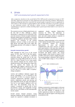
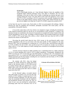
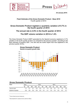


© Copyright 2026