1. Art and Diseño

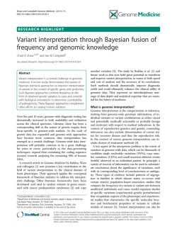
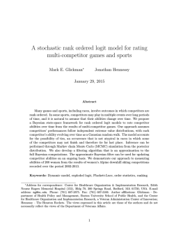
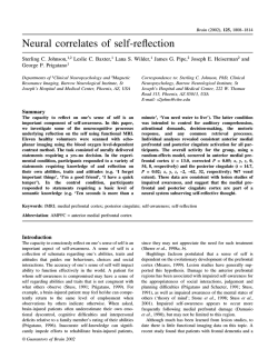
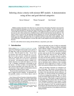
Belief Flows for Robust Online Learning
Pedro A. Ortega
Koby Crammer
Daniel D. Lee
School of Engineering
and Applied Sciences
University of Pennsylvania
Philadelphia, PA 19104, USA
Email: [email protected]
Department of
Electrical Engineering
The Technion
Haifa, 32000 Israel
Email: [email protected]
School of Engineering
and Applied Sciences
University of Pennsylvania
Philadelphia, PA 19104, USA
Email: [email protected]
Abstract— This paper introduces a new probabilistic model
for online learning which dynamically incorporates information
from stochastic gradients of an arbitrary loss function. Similar
to probabilistic filtering, the model maintains a Gaussian belief
over the optimal weight parameters. Unlike traditional Bayesian
updates, the model incorporates a small number of gradient evaluations at locations chosen using Thompson sampling, making it
computationally tractable. The belief is then transformed via a
linear flow field which optimally updates the belief distribution
using rules derived from information theoretic principles. Several
versions of the algorithm are shown using different constraints
on the flow field and compared with conventional online learning
algorithms. Results are given for several classification tasks
including logistic regression and multilayer neural networks.
I. I NTRODUCTION
An number of problems in artificial intelligence must cope
with continual learning tasks involving very large datasets or
even data streams which have become ubiquitous in application domains such as life-long learning, computer vision,
natural language processing, bioinformatics and robotics. As
these big-data problems demand richer models, novel online
algorithms are needed that scale efficiently both in accuracy
and computational resources. Recent work have shown that
complex models require regularization to avoid local minima
and overfitting—even when the data is abundant [1].
The aim of our work is to formulate an efficient online
learning approach that leverages the advantages of stochastic
gradient descent (SGD) [2] and Bayesian filtering [3]. Many
learning tasks can be cast as optimization problems, and SGD
is simple, scalable and enjoys strong theoretical guarantees in
convex problems [4], [5] but tends to overfit if not properly
regularized. On the other hand, Bayesian filtering methods
track belief distributions over the optimal parameters to avoid
overfitting, but are typically computationally prohibitive for
rich models. To combine these two approaches, we had to
address two questions.
The first question is how to update a global belief distribution over optimal parameters from a local update prescribed
by SGD. In other words, rather than calculating the posterior
using a likelihood function, we take gradients as directly
specifying the velocity field—or flow field—of belief updates.
As shown in Figure 1, this can be viewed as tracking an
ensemble of models under the dynamics induced by the
expected prediction error. We answer this question by using
a)
b)
c)
Fig. 1. Schematic comparison of learning dynamics in (a) stochastic gradient
descent, (b) Bayesian filtering, and (c) belief flows.
the principle of minimum information discrimination (MID)
[6] to choose the most conservative posterior belief that is
consistent with the gradient measurement and assumptions on
the flow field.
The second question is how to generate predictions without
integrating over the parameter uncertainty. Calculating the
optimal belief update would require estimating the expected
SGD update at every point in parameter space, which is
prohibitive. To overcome this problem, a natural choice is to
use Thompson sampling, i.e. sampling parameters from the
posterior according to the probability of being optimal [7]. As
is well known in the literature in Bayesian optimization [8],
optimizing the parameters of an unknown and possibly nonconvex error function requires dealing with the explorationexploitation trade-off, which is precisely where Thompson
sampling has been shown to outperform most state-of-the-art
methods [9].
Here, we illustrate this modelling approach by deriving the
update rules for Gaussian belief distributions over the optimal
parameter. By assuming that observations generate linear flow
fields, we furthermore show that the resulting update rules
have closed-form solutions. Because of this, the resulting
learning algorithms are online, permitting training examples
to be discarded once they have been used.
II. G AUSSIAN B ELIEF F LOWS
We focus on prediction tasks with parameterized models,
each denoted by Fw (x) with inputs x ∈ Rp and parameters
w ∈ Rd . At each round n = 1, 2, . . . the algorithm maintains a
belief distribution Pn (w) over the optimal parameters. Here we
choose Pn (w) to be represented by a d-dimensional Gaussian
with mean µn and covariance Σn :
Pn (w) = N (w; µn , Σn )
1
1
T −1
exp − (w − µn ) Σn (w − µn ) .
=p
2
(2π)d detΣn
In each round, the algorithm samples a parameter vector
wn from the distribution Pn (w). The components of wn
are then used as parameters in a classification or regression
machine for a given input xn . For example, we can consider
logistic regression where wn are the parameters of the logistic
function. Or we can use deep networks, where wn specifies
the synaptic weights of the different layers of the network.
Without loss of generality, this yields a prediction yˆn for the
particular input xn :
yˆn = Fwn (xn ).
A supervised output signal yn is also provided, and we wish
to minimize the loss between the true output and predicted
output:
`(yn , yˆn ).
To improve the loss on the current example, SGD then updates
the parameter as:
∂
`(yn , yˆn )|w=wn ,
(1)
∂w
where η > 0 is a learning rate which may vary as the number
of rounds increase. For the case of a multilayer perceptron,
this gradient can be efficiently computed by the well-known
backpropagation algorithm in a single backwards pass.
wn0 = wn − η ·
A. Full Flow
Knowing that the sampled parameter vector wn needs to be
modified to wn0 , how do we choose the posterior Pn+1 (w)? To
answer this question, we assume that the update results from
a linear flow field, i.e. each w ∈ Rd is updated as
0
w = Aw + b
d×d
where A ∈ R
is an affine transformation matrix and b ∈ Rd
is a translational offset. The main advantage of a linear flow is
that Gaussian distributions remain Gaussian under such a field
[10]. In particular, we choose the flow parameters to match the
SGD update (1):
wn0 = Awn + b.
(2)
Under this linear flow, the new belief distribution is
Pn+1 (w) = N (Aµn + b, AΣn AT ) = N (µn+1 , Σn+1 )
where the mean is shifted to µn+1 = Aµn + b and the
covariance is scaled to Σn+1 = AΣn AT . There are many
potential A and b which satisfy the flow constraint in (2), so
we need a way to regularize the ensuing distribution Pn+1 (w).
We utilize the Kullback-Leibler divergence
Z
Pn+1 (w)
min DKL [Pn+1 kPn ] = min Pn+1 (w) log
dw.
A,b
A,b
Pn (w)
(3)
subject to the constraint wn0 = Awn + b. This is an application
of the principle of MID [6], an extension of the maximum
entropy principle [11], and governs the updates of exponential
family distributions [12]. The next theorem (see the S.M. for
the proof) shows that this problem has a closed-form solution.
Theorem 1: Let Σn = Un Dn UnT be the eigendecomposition of the covariance matrix. Let
1
uˆ
µ = √ UnT (wn − µn )
Dn
1
vk µ
ˆ + v⊥ νˆ = √ UnT (wn0 − µn )
Dn
be the transformed (whitened) differences between the sampled parameter vector and the mean before and after the update
respectively, expressed in terms of the 2-D basis spanned by
the unitary orthogonal vectors µ
ˆ and νˆ. Then, the solution A∗
to (3) is
T p
1
µ
ˆ
√ UnT
ˆ νˆ (A2×2 − I2×2 )
Id×d + Un Dn µ
νˆT
Dn
where the 2-D transformation matrix A2×2 is given by
 q 2 2
q
2
2
u
1

q

2
2
vk + v⊥
u
vk +v⊥ +δ1
4+u2 (4+vk +v⊥ )
2)
2(1+u
q
q
2 +δ
2 )
vk2 +v⊥
4+u2 (4+vk2 +v⊥
1
2(1+u2 )
vk
v⊥

−δ2 v⊥ 

+δ2 vk
δ1 , δ2 ∈ {−1, +1}. The hyperparameters of the posterior
distribution are then equal to
Σn+1 = A∗ Σn A∗T
µn+1 = A∗ (µn − wn ) + wn0 .
There are actually four discrete solution to (3), one for each
combination of δ1 and δ2 . If we assume that the SGD learning
rate is small, then wn0 − µn ≈ wn − µn . In this case, we
should choose the solution A∗ ≈ Id×d obtained by selecting
δ1 = δ2 = 1.
B. Diagonal and Spherical Flows
We now consider two special cases: flows with diagonal and
spherical transformation matrices, i.e. of the form
A = diag(a1 , a2 , . . . , ad ) and A = aU,
where diag(v) denotes the square diagonal matrix with the elements of the vector v on the main diagonal and U is a unitary
(rotation) matrix. We match these flow types with multivariate
Gaussians having diagonal and spherical covariance matrices.
Let N (µ, Σ) be the prior and N (µ0 , Σ0 ) be the posterior at
round n, and let subindices denote vector components in the
following.
a) Diagonal:: For the diagonal case, the multivariate
distribution N (µ, Σ) factorizes into d univariate Gaussians
N (µi , σi2 ) that can be updated independently under flow fields
of the form
wi0 = ai wi + bi .
(4)
Under these constraints, it can be shown (see S.M.) that the
optimal transformation is given by
p
ui vi + δi 4 + u2i (4 + vi2 )
∗
ai =
,
2(1 + u2i )
where ui = (wi − µi )/σi , vi = (wi0 − µi )/σi are the i-th
component of the normalized sampled parameter before and
after updating and δi ∈ {−1, +1}. Similarly to the general
case, we choose the solution closer to the identity when ui ≈
vi by picking δi = +1. The posterior hyperparameters are
σi0 = a∗i σi
µ0i
µ0i = a∗i (µi − wi ) + wi0 .
(5)
σi0
where
and
are the new mean and standard deviation of
the i-th component.
b) Spherical:: For the spherical case, the flow field that
preserves the spherical distribution is of the form A = aU ,
where a > 0 is a scalar and U is a unitary matrix such that
A(w − µ) and (w0 − µ) are colinear; that is, A rotates and
scales (w − µ) to align it to (w0 − µ). The update is
w0 = aw + b,
(6)
that is, similar to (4) but with an isotropic scaling factor a.
The optimal scaling factor is then given by
p
uv + δ 4 + u2 (4 + v 2 )
∗
,
a =
2(1 + u2 )
0
where u = (kw − µk)/σ, v = (kw − µk)/σ, where
δ ∈ {−1, +1} is choosen as δ = 1 for the near-identity
transformation.
C. Non-Expansive Flows
The previously derived update rules allow flow fields to
be expansive, producing posterior distributions having larger
differential entropy than the prior. Such flow fields are needed
when the error landscape is dynamic, e.g. when the data is
nonstationary. However, for faster convergence with stationary
distributions, it is desirable to restrict updates to non-expansive
flows. Such flow fields are obtained by limiting the singular
values of the transformation matrix A to values that are smaller
or equal than one.
D. Implementation
The pseudocode of a typical gradient-based online learning
procedure is listed in Algorithm 1. For a d-dimensional
multivariate Gaussian with diagonal and spherical covariance
matrix, the update has time complexity O(d), while for an
unconstrained covariance matrix, this update is O(d3 ) in a
naive implementation performing a spectral decomposition in
each iteration. The complexity of the unconstrained covariance
implementation can be reduced using low-rank techniques as
described in [13]. Numerically, it is important to maintain the
positive semidefiniteness of the covariance matrix. One simple
way to achieve this is by constraining its eigenvalues to be
larger than a predefined minimum.
III. P ROPERTIES
A. Comparison
The full optimal transformation will include rotations in the
2-D subspace spanned by the sampled and learned parameter
vectors. In contrast, the diagonal transformation will only
scale and translate each basis direction independently, and
Algorithm 1 BFLO Pseudo-Code
Input: µ1 , Σ1 , hyperparameters
for n = 1, 2, . . . , N do
Get training example (xn , yn ).
Calculate output:
Sample wn ∼ N (µn , Σn )
Set zn ← Fw (xn )
Local flow:
Calculate new weights using e.g. gradient descent,
∂`
(yn , zn )|wn
wn0 ← wn − η ∂w
Global flow:
Calculate flow matrix A? (full, diagonal or spherical).
Update hyperparameters:
Σn+1 ← A? Σn A?T
µn+1 ← A? (µn − wn ) + wn0
(Optional) perform numerical correction.
end for
Return (µN , ΣN )
the spherical transformation acts on the radial parameter only.
Since rotations allow for more flexible transformations, the
full flow update will keep the belief distribution relatively
unchanged, while the diagonal and spherical flows will force
the belief distribution to shift and compress more. The update
that is better at converging to an optimal set of weights is
problem dependent. The three update types are shown in
Figure 2a.
B. Update Rule
To strenghten the intuition, we briefly illustrate the nontrivial effect that the update rule has on the belief distribution.
Figure 2b shows the values of the posterior hyperparameters
of a one-dimensional standard Gaussian as a function of ∆ =
(w − µ) and ∆0 = (w0 − µ), that is, the difference of the
sampled weight and the center of the prior Gaussian before
and after the update.
Roughly, there are three regimes, which depend on the
displacement ∆0 − ∆ = w0 − w. First, when the displacement
moves towards the prior mean without crossing it, then the
variance decreases. This occurs when 0 ≤ ∆0 ∆ ≤ ∆2 , that is,
below the diagonal in the first quadrant and above the diagonal
in the third quadrant. Second, if the displacement crosses the
prior mean, then the flow field is mainly explained in terms
of a linear translation of the mean. This corresponds to the
second and fourth quadrants. Finally, when the displacement
moves away from the prior mean, the posterior mean follows
the flow and the variance increases. This corresponds to the
regions where ∆2 < ∆0 ∆, i.e. above the diagonal in the first
and below the diagonal in the third quadrant.
Note that the diagonal ∆0 = ∆ leaves the two hyperparameters unchanged, and that the vertical ∆ = 0 does not lead to a
change of the variance. Figure 2c illustrates the change of the
prior into a posterior belief. The left panel shows the update of
a sampled weight equal to the standard deviation, and the right
panel show the update for a sampled weight equal to one-fifth
a)
Full Flow
b)
Spherical Flow
Diagonal Flow
2
5
5
2.5
5
0
1.5
1.5
-5
1
0.5
0.5
0
0
0
−0.5
−1
−1.5
−2
−2
−1
0
1
2
−2
−1
0
1
−2
2
−1
0
1
2
-5
-5
0
5
-5
-5
0
5
c)
1
1
0.8
0.8
0.6
0.6
0.4
0.4
0.2
0.2
0
-5
0
5
0
-5
0
5
Fig. 2. a) Comparison of different flow types. b) 1-D Update of the mean µ = 0 and standard deviation σ = 1 as a function of ∆ = (w − µ) and
∆0 = (w0 − µ). b) The two panels illustrate the posterior beliefs (red) resulting from updating a 1-D prior (black) by moving a sampled weight through
displacements in {−4, −2, +2, +4}. The prior and posterior positions of the sampled weight are indicated with dashed vertical lines.
50 Rounds
2
1
1
0.5
0.5
ift
dr
0
-0.5
-0.5
-1
-1
-1.5
-1.5
-2
-2
(subtraction) of datapoints that attract (repel) the mean shown
in black by relocating the center of mass. In the figure,
blue and red correspond to added and subtracted datapoints
respectively, and the circular areas indicate their precision,
i.e. ρn = 1/λn , where λn ∈ R is the unique eigenvalue of
R at round n. The convergence of the belief distribution to a
particular point z ∈ Rd can thus be analyzed in terms of the
convergence of the weighted average of the P
pseudo datapoints
to z and accumulation of precision, that is n ρn → +∞.
1.5
1.5
0
300 Rounds
2
optimum
-1
0
Fig. 3.
1
2
-2
-2
optimum
-1
0
1
2
Evolution of Pseudo Dataset
of the standard deviation. Here, it is seen that if the sampled
weight is closer to the mean, then the update is reflected in a
mean shift with less change in the variance.
C. Pseudo Datasets
The belief updates can be related to Bayesian updates
through (pseudo) datapoints that would yield the same posterior. Since a belief flow update ensures that the posterior
stays within the Gaussian family, it is natural to relate it
to Bayesian estimation of an unknown mean (but known
covariance) under the self-conjugate Gaussian family. More
precisely, let P (w) = N (w; µ, Σ) and P 0 (w) = N (w; µ0 , Σ0 )
denote the prior and the posterior of a belief flow update. Then,
it is easily verified that this is equivalent to conditioning a
prior P (w) = N (w; µ, Σ) on a point u ∈ Rd with likelihood
function P (x|w) = N (x; w, R), where
x = (Σ0−1 − Σ−1 )−1 (Σ0−1 µ0 − Σ−1 µ),
0−1
R = (Σ
−Σ
−1 −1
)
.
(7)
(8)
The matrix R is symmetric but not necessarily positive
semidefinite unless we use non-expansive flows. A negative
eigenvalue λ of R then indicates an increase of the variance
along the direction of its eigenvector vλ ∈ Rd . From a
Bayesian point of view, this implies that the pseudo datapoint
was removed (or forgotten), rather than added, along the
direction of vλ . We have already encountered this case in the
1-D case in Section III-B when the posterior variance increases
due to a displacement that points away from the mean.
Figure 3 shows the pseudo dataset for a sequence of updates
of a spherical belief flow. The temporal dynamics of the
belief distribution can be thought of as driven by the addition
IV. E MPIRICAL E VALUATION
We evaluated the diagonal variant of Gaussian belief flows
(BFLO) on a variety of classification tasks by training logistic regressors and multilayer neural networks. These results
were compared to several baseline methods, most importantly
stochastic gradient descent (SGD). Our focus in these experiment was not to show better performance to existing learning
approaches, but rather to illustrate the effect of different regularization schemes over SGD. Specifically, we were interested
in the transient and steady-state regimes of the classifiers to
measure the online and generalization properties respectively.
Here we summarize the main results and refer the reader to
the S.M. for further details.
A. Logistic Regression
For this model, we compared Gaussian belief flows (BFLO)
on several binary classification datasets and compared its performance to three learning algorithms: AROW [14], stochastic
gradient descent (SGD) and Bayesian Langevin dynamics
(BLANG) [1]. With the exception of AROW, which combines
large margin training and confidence weighting, these are
all gradient-based learning algorithms. The algorithms were
used to train a logistic regressor described as follows. The
probability of the output y ∈ {0, 1} given the corresponding
input x ∈ R2 is modelled as
P (y = 1|x) = σ(wT x),
(9)
1
where w ∈ R2 is a parameter vector and σ(t) = 1+exp(−t)
is the logistic sigmoid. When used in combination with the
binary KL-divergence1
`(z, y) = y log
y
(1 − y)
+ (1 − y) log
z
(1 − z)
(10)
1 Equivalently, one can use the binary cross-entropy defined as `(y, z) =
−y log z − (1 − y) log(1 − z).
TABLE II
MNIST C LASSIFICATION R ESULTS
as the error function, the error gradients become:
∂`
= (z − y)x.
∂w
(11)
We measured the online and generalization performance in
terms of the number of mistakes made in a single pass through
80% of the data and the average classification error without
updating on the remaining 20% respectively. Additionally, to
test robustness to noise, we repeated the experiments, but
inverting the labels on 20% of the training examples (the
evaluation was still done against the true labels).
To test the performance in the online setting, we selected
well-known binary classification datasets having a large number of instances, summarized as follows. MUSHROOM:
Physical characteristics of mushrooms, to be classified into
edible or poisonous. This UCI dataset contains 8124 instances
with 22 categorical attributes each that have been expanded
to a total of 112 binary features2 . COVTYPE: 581,012 forest
instances described by 54 cartographic variables that have to
be classified into 2 groups of forest cover types [15]. IJCNN:
This is the first task of the IJCNN 2001 Challenge [16]. We
took the winner’s preprocessed dataset [17], and balanced
the classes by using only a subset of 27,130 instances of
22 features. EEG: This nonstationary time series contains a
recording of 14,980 samples of 14 EEG channels. The task
is to discriminate between the eye-open and eye-closed state3 .
A9A: This dataset, derived from UCI Adult [18], consists of
32,561 datapoints with 123 features from census data where
the aim is to predict whether the income exceeds a given
threshold.
We used grid search to choose simple experimental parameters that gave good results for SGD, and used them
on all datasets and gradient-based algorithms to isolate the
effect of regularization. In particular, we avoided using popular
tricks such as “heavy ball”/momentum [19], minibatches, and
scheduling of the learning rate. SGD and BLANG were
initialized with parameters drawn from N (0, σ 2 ) and BFLO
with a prior equal to N (0, σ 2 ), where σ = 0.2. The learning
rate was kept fixed at η = 0.001. For the AROW parameter
we chose r = 10. With the exception of EEG, all datasets
were shuffled at the beginning of a run.
Table I summarizes our experimental results averaged over
10 runs. The online classification error is given within a
standard error σerr < 0.01. The last column lists the mean
rank (out of 4, over all datasets), with 1 indicating an algorithm
attaining the best classification performance. BFLO falls short
in convergence speed due to its exploratory behavior in the
beginning, but then outperforms the other classifiers in its
generalization ability. Compared to the other methods, it
comes closest to the performance of BLANG, both in the
transient and in the steady-state regime, and in the remarkable
robustness to noise. This may be because both methods use
Monte Carlo samples of the posterior to generate predictions.
2 http://www.csie.ntu.edu.tw/
Online Classification Error in %
RANDOM
0.96
IMAGES
1.16
Rank
max{σerr }
PLAIN
0.07
SGD
DROPOUT
BFLO
11.25
9.84
11.01
89.14
52.87
37.94
72.41
50.68
47.71
3.0
1.6
1.3
RANDOM
3.33
IMAGES
6.05
Rank
max{σerr }
PLAIN
0.44
SGD
DROPOUT
BFLO
7.01
5.52
5.00
89.17
53.42
29.11
65.17
46.67
41.55
3.0
2.0
1.0
Final Classification Error in %
B. Feedforward Neural Networks
This experiment investigates the application of Belief Flows
to learn the parameters of a more complex learning machine—
in this case, a feedforward neural network with one hidden
layer. We compared the online performance of Gaussian belief
flows (BFLO) to two learning methods: plain SGD and SGD
with dropout [20]. As before, our aim was to isolate the effect
of the regularization methods on the online and test performance by choosing a simple experimental setup with shared
global parameters, avoiding architecture-specific optimization
tricks.
We tested the learning algorithms on the well-known
MNIST4 handwritten digit recognition task (abbreviated here
as BASIC), plus two variations derived in [21]: RANDOM:
MNIST digits with a random background, where each random
pixel value was drawn uniformly; IMAGES: a patch from a
black and white image was used as the background for the digit
image. All datasets contained 62,000 grayscale, 28 × 28-pixel
images (totalling 784 features). We split each dataset into an
online training set containing 80% and a test set having 20%
of the examples.
To attain converging learning curves in the (single-pass)
online setting, we have chosen a modest architecture of 784
inputs, 200 hidden units and 10 outputs with aggressive
updates. All units have a logistic sigmoid activation function,
and error gradients were evaluated on the binary KullbackLeibler divergence function averaged over the outputs. At the
beginning of each run, the examples were shuffled and the
training initialized with weights either drawn independently
from a normal N (0, σ 2 ) (SGD and dropout) or by setting
the prior to N (0, σ 2 ) (BFLO), where σ = 0.1. Throughout
the online learning phase, the learning rate was kept fixed at
η = 0.2 and we applied 5 update iterations on each example
before discarding it.
We report the results in Table II which were averaged
over 5 runs. As the level of noise increased, all the classifiers
declined in performance, with PLAIN being the easiest and
RANDOM being the hardest to learn. SGD had a particularly
poor behavior relative to the regularized learners with their
cjlin/libsvmtools/datasets/binary.html
3 https://archive.ics.uci.edu/ml/datasets/EEG+Eye+State
4 http://yann.lecun.com/exdb/mnist/index.html
TABLE I
B INARY C LASSIFICATION R ESULTS FOR N OISE L EVELS 0%/20%
Online Classification Error in %
MUSHR.
COVTYPE
IJCNN
EEG
A9A
Rank
5.32/11.05
11.86/11.05
14.44/14.35
14.30/15.34
22.58/23.10
28.03/28.18
29.30/29.44
28.14/28.39
8.44/17.38
9.01/9.87
12.86/12.06
10.34/11.52
43.59/45.11
43.39/44.22
43.71/44.20
44.07/44.37
17.79/20.95
18.62/18.48
20.51/20.20
19.03/19.04
1.2/2.8
1.8/1.6
3.2/2.8
3.8/2.8
COVTYPE
0.12/0.40
IJCNN
0.26/1.23
EEG
0.69/1.26
A9A
0.08/0.12
Rank
max{σerr }
MUSHR.
0.23/0.32
AROW
SGD
BLANG
BFLO
9.59/13.77
5.35/10.78
1.16/0.34
1.79/0.65
37.18/38.11
37.45/38.36
38.39/39.09
37.03/37.69
20.10/20.28
19.10/26.52
15.97/14.60
16.92/16.67
65.38/63.09
60.57/61.24
64.85/66.68
62.76/62.35
15.85/17.56
17.45/19.32
17.68/19.58
17.00/16.69
3.0/2.8
2.6/2.8
2.6/2.8
1.8/1.6
AROW
SGD
BLANG
BFLO
Final Classification Error in %
built-in mechanisms to avoid local minima. BFLO attained
the lowest error rates both online and in generalization.
Interestingly, it copes better with the RANDOM than with
the IMAGES dataset. This could be because Monte Carlosampling smoothens the gradients within the neighborhood.
future theoretical work includes analyzing regret bounds, and a
more in-depth investigation of the relation between stochastic
approximation, reinforcement learning and Bayesian methods
that are synthesized in a belief flow model.
R EFERENCES
V. D ISCUSSION AND F UTURE W ORK
Our experiments indicate that Belief Flows methods are
suited for difficult online learning problems where robustness
is a concern. Gaussian belief flows may be related to ensemble
learning methods in conjunction with locally quadratic cost
functions. A continous ensemble of predictors that is trained
under gradient descent follows a linear velocity field when
the objective function is a quadratic form. Under such flow
fields, the Gaussian family is a natural choice for modelling
the ensemble density since it is invariant to linear velocity
fields. An iteration of the update rule then infers the dynamics
of the whole ensemble from a single sample by conservatively
estimating the ensemble motion in terms of the KullbackLeibler divergence.
Following the Bayesian rationale, the resulting predictor
is an ensemble rather than a single member. Any strategy
deciding which one of them to use in a given round must
deal with the exploration-exploitation dilemma; that is, striking
a compromise between minimizing the prediction error and
trying out new predictions to further increase knowledge [22].
This is necessary to avoid local minima–here we sample a
predictor according to the probability of it being the optimal
one, a strategy known as Thompson sampling [7], [23], [24].
The maintainence of a dynamic belief in this manner allows
the method to outperform algorithms that maintain only a
single estimate in complex learning scenarios.
The basic scheme presented here can be extended in many
ways. Some possibilities include the application of Gaussian belief flows in conjunction with kernel functions and
gradient acceleration techniques, and in closed-loop setups
such as in active learning. Furthermore, linear flow fields can
be generalized by using more complex probabilistic models
suitable for other classes of flow fields following the same
information-theoretic framework outlined in our work. Finally,
[1] M. Welling and Y.-W. Teh, “Bayesian Learning via Stochastic Gradient
Langevin Dynamics,” in ICML, 2011.
[2] H. Robbins and S. Monro, “A Stochastic Approximation Method,”
Annals of Mathematical Statistics, vol. 22, no. 3, pp. 400–407, 1951.
[3] S. S¨arkk¨a, Bayesian Filtering and Smoothing, ser. Institute of Mathematical Statistics Textbooks. Cambridge University Press, 2013.
[4] L. Bottou, “Large-scale machine learning with stochastic gradient descent,” in Proceedings of COMPSTAT’2010. Springer, 2010, pp. 177–
186.
[5] F. Bach and E. Moulines, “Non-Asymptotic Analysis of Stochastic
Approximation Algorithms for Machine Learning,” in NIPS, 2011.
[6] S. Kullback, Information Theory and Statistics. New York: Wiley, 1959.
[7] W. Thompson, “On the likelihood that one unknown probability exceeds
another in view of the evidence of two samples,” Biometrika, vol. 25,
no. 3/4, pp. 285–294, 1933.
[8] J. Mockus, “Bayesian Approach to Global Optimization: Theory and
Applications,” 2013.
[9] O. Chapelle and L. Li, “An Empirical Evaluation of Thompson Sampling,” in NIPS, 2011.
[10] K. Crammer and D. D. Lee, “Learning via Gaussian Herding,” in NIPS,
2010, pp. 451–459.
[11] E. Jaynes, “Information Theory and Statistical Mechanics,” Physical
Review. Series II, vol. 106, no. 4, pp. 620–630, 1957.
[12] I. Csisz´ar and P. Shields, Information Theory and Statistics: A Tutorial.
Now Publishers Inc, 2004.
[13] J. R. Bunch, C. P. Nielsen, and D. C. Sorensen, “Rank-one modification
of the symmetric eigenproblem,” Numerische Mathematik, vol. 31, no. 1,
pp. 31–48, 1978.
[14] K. Crammer, A. Kulesza, and M. Dredze, “Adaptive Regularization of
Weighted Vectors,” in NIPS, 2009.
[15] R. Collobert, S. Bengio, and Y. Bengio, “A parallel mixture of SVMs
for very large scale problems,” Neural Computation, vol. 14, no. 05, pp.
1105–1114, 2002.
[16] D. Prokhorov, “IJCNN 2001 neural network competition,” 2001.
[17] C.-C. Chang and C.-J. Lin, “IJCNN 2001 challenge: Generalization
ability and text decoding,” in IJCNN. IEEE, 2001.
[18] C.-J. Lin, R. C. Weng, and S. S. Keerthi, “Trust region Newton
method for large-scale logistic regression,” Journal of Machine Learning
Research, vol. 9, pp. 627—–650, 2008.
[19] B. T. Polyak, “Some methods of speeding up the convergence of iteration
methods,” Zh. Vychisl. Mat. Mat. Fiz., vol. 4, no. 5, pp. 791–803, 1964.
[20] G. E. Hinton, N. Srivastava, A. Krizhevsky, I. Sutskever, and R. R.
Salakhutdinov, “Improving neural networks by preventing co-adaptation
of feature detectors,” arXiv:1207.0580, 2012.
[21] H. Larochelle, D. Erhan, A. Courville, B. J., and Y. Bengio, “An
empirical evaluation of deep architectures on problems with many
factors of variation,” in ICML 2007, 2007.
[22] R. Sutton and A. Barto, Reinforcement Learning: An Introduction.
Cambridge, MA: MIT Press, 1998.
[23] M. Strens, “A Bayesian framework for reinforcement learning,” in
ICML, 2000.
[24] P. A. Ortega and D. A. Braun, “A minimum relative entropy principle for
learning and acting,” Journal of Artificial Intelligence Research, vol. 38,
pp. 475–511, 2010.