1. Art and Diseño

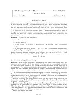
Correlated equilibria in homogenous good Bertrand
competition∗
Ole Jann and Christoph Schottmu
¨ller†
January 29, 2015
Abstract
We show that there is a unique correlated equilibrium, identical to the unique
Nash equilibrium, in the classic Bertrand oligopoly model with homogenous goods
and identical marginal costs. This provides a theoretical underpinning for the socalled “Bertrand paradox” as well as its most general formulation to date. Our
proof generalizes to asymmetric marginal costs and arbitrarily many players in
the following way: The market price cannot be higher than the second lowest
marginal cost in any correlated equilibrium.
JEL: C72, D43, L13
Keywords: Bertrand paradox, correlated equilibrium, price competition
1. Introduction
A substantial body of theory in industrial organization and other fields of economics is
built on the idea that there are no equilibria with positive expected profits in a simple
Bertrand competition model with homogenous goods and symmetric firms—in other
∗
The authors would like to thank one anonymous referee and the editor (Atsushi Kajii) for helpful
suggestions. We have also benefitted from comments by Jan Boone, Gregory Pavlov and Peter Norman
Sørensen.
†
Address to both authors: Department of Economics, University of Copenhagen, Øster Farimagsgade 5, Building 26, DK-1353 Copenhagen K, Denmark; email:
[email protected].
1
[email protected] and
words, that there are no profitable cartels and that price competition between n > 1
firms will drive prices down to marginal cost in one-shot price competition. The fact
that price competition between two firms is equivalent to perfect competition is often
referred to as the “Bertrand paradox”.
Yet the theoretical foundation for this idea is not fully clear, especially where correlated equilibria are concerned. In a correlated equilibrium, players can construct a
correlation device which gives each player a private recommendation before the players
choose their actions. In correlated equilibrium, the device is such that it is an equilibrium
for the players to follow the recommendation. Every (mixed strategy) Nash equilibrium
is a correlated equilibrium where the recommendations are independent. Players can
in many games achieve higher payoffs in correlated equilibrium than in Nash equilibrium because the device is able to correlate recommendations; see Aumann (1974). In
Bertrand competition, it is conceivable that players could correlate their prices in such
a way as to achieve high prices while still (through the shape of the joint price distribution) making sure that none of them wants to deviate. We show that this is not possible,
although the argument is somewhat subtle.
More precisely, we show that no correlated equilibrium (and hence also no mixed
Nash equilibrium) with positive expected profits can exist in a symmetric Bertrand game
with homogenous products and bounded monopoly profits.1 This is the most general
formulation of the Bertrand paradox yet. Our result is certainly desirable because
a statement like the Bertrand paradox – implying that zero profits are inevitable in a
price competition setting – should naturally be shown using an equilibrium concept that
is “permissive”, i.e. a solution concept that allows the players to coordinate as much as
possible within the paradigm of a one-shot, non-cooperative game. This is exactly what
correlated equilibrium does.2 Our result is not obvious given that the set of rationalizable
1
Wu (2008) claims to prove a similar theorem for symmetric linear costs and linear demand. Note,
however, that he does not provide a proof for the central second case in his case distinction and
implicitly limits his analysis to a finite action space which is incompatible with the standard version of
the Bertrand game.
2
Correlated equilibrium has been shown to have many other attractive properties as well: For
example, several simple learning procedures converge to correlated equilibria, see for example Foster
and Vohra (1997), Fudenberg and Levine (1999), Hart and Mas-Colell (2000), and unique correlated
equilibria are robust to introducing incomplete information, see Kajii and Morris (1997). It should,
2
actions is large: In symmetric, homogenous good Bertrand competition all non-negative
prices are rationalizable.3 This is, for example, in stark contrast to Bertrand games
with differentiated products: Milgrom and Roberts (1990) show for a large class of
demand functions that there is a unique rationalizable action in a differentiated goods
Bertrand game. This clearly implies that there is a unique Nash equilibrium and also
a unique correlated equilibrium in these games. Their reasoning, however, applies only
to supermodular games. A Bertrand game with homogenous goods is not supermodular
since the profit functions (i) do not have increasing differences and (ii) are not order
upper semi-continuous in the firm’s price.
Our proof is by contradiction: We show that if there was a correlated equilibrium in
which prices higher than marginal cost were played with positive probability, then there
would be an interval of recommendations in which each player prefers to deviate downwardly from his recommendation. This interval consists of the highest recommendations
that a player might get (with positive probability) in the assumed equilibrium.
The contribution of this paper lies in the proof that in Bertrand games with arbitrary
demand functions (in which the set of rationalizable actions is infinite), the Bertrand
Nash equilibrium is the unique correlated equilibrium.
Apart from that, it is also a generalization (by different methods) of results of Baye
and Morgan (1999) and Kaplan and Wettstein (2000) on mixed-strategy equilibria in
Bertrand games. Baye and Morgan (1999) show that if monopoly profits are unbounded,
any positive finite payoff vector can be achieved in a symmetric mixed-strategy Nash
equilibrium, and Kaplan and Wettstein (2000) prove that unboundedness of monopoly
profits is both necessary and sufficient for the existence of such mixed-strategy Nash
equilibria. These insights have led Klemperer (2003, section 5.1) to conclude that “there
are other equilibria with large profits, for some standard demand curves.” We show that
expected profits in any correlated equilibrium (and therefore in any mixed Nash equilibrium) are zero if demand is such that monopoly profits are bounded. Finally, unlike the
cited results, our proof is generalizable to games with asymmetric costs and arbitrarily
many players: We show that the highest market price in any correlated equilibrium
however, be noted that these papers limit themselves to finite games for technical reasons.
3
Every pi ∈ R+ is in our model rationalizable because pi is – assuming zero marginal costs – a best
response to pj = 0 which is the Bertrand equilibrium price and therefore itself rationalizable.
3
equals the second lowest marginal cost. This establishes an (outcome) equivalence of
Nash and correlated equilibria also in this more general setup.
A related result is derived in Liu (1996). Liu shows that the unique Nash equilibrium
in Cournot competition with linear demand and constant marginal costs is also the
unique correlated equilibrium.
This paper is organized as follows. The next section introduces the Bertrand model
with two symmetric firms as well as the concept of correlated equilibrium. Section 3
derives our result. This result is generalized for the case of n non-symmetric firms in
section 4. Section 5 concludes.
2. Model
There are two firms with constant marginal costs which are normalized to zero. Firms
set prices simultaneously. The price of firm i is denoted by pi . If pi < pj , consumers buy
quantity D(pi ) of the good from firm i (and 0 units from firm j). If both firms quote
the same price p0 , consumers buy D(p0 )/2 from each firm. D(p) denotes market demand
where D : R+ → R+ is a (weakly) decreasing, measurable function and R+ denotes the
non-negative real numbers. We assume that the demand function is such that a strictly
positive monopoly price arg maxp pD(p) exists. We define pmon as the supremum of
all prices maximizing pD(p) and assume that pmon is finite. Firms maximize expected
profits.
A correlated equilibrium in this game is a probability distribution F on R+ × R+ .
This probability distribution is interpreted as a correlation device. The correlation
device sends recommended prices (r1 , r2 ) to the two firms. Each firm i observes ri but
does not observe the other firm’s recommendation rj . F (p1 , p2 ) is the probability that
(r1 , r2 ) ≤ (p1 , p2 ). Roughly speaking, a distribution F is called a correlated equilibrium
if both firms find it optimal to follow the recommendation.
To be more precise denote the profits of firm i given prices pi and pj with i, j ∈ {1, 2}
4
and i 6= j as



pi D(pi )



πi (pi , pj ) = pi D(pi )/2





0
if pi < pj
if pi = pj
(1)
else.
Note that we define the profit function such that the own price is the first argument,
i.e. the first argument of π2 is p2 .
A strategy for firm i is a mapping from “recommendations” to prices. Both recommendations and prices are in R+ . Hence, a strategy is a measurable function ζi : R+ →
R+ . The identity function represents the strategy of following the recommendation. F
is a correlated equilibrium if no firm can gain by unilaterally deviating from a situation
where both firms use ζi = identity function. More formally, we follow the definition of
correlated equilibrium for infinite games given in Hart and Schmeidler (1989) and also
used in Liu (1996): A correlated equilibrium is a distribution F on R+ × R+ such that
for all measurable functions ζi : R+ → R+ and all i ∈ {1, 2} and i 6= j ∈ {1, 2} the
following inequality holds:
Z
πi (pi , pj ) − πi (ζi (pi ), pj ) dF (p1 , p2 ) ≥ 0.
(2)
R+ ×R+
In words, a distribution F is a correlated equilibrium if no player can achieve a higher
expected payoff by unilaterally deviating to a strategy ζi instead of simply following the
recommendation. Last, we define a symmetric correlated equilibrium as a correlated
equilibrium F in which F (p1 , p2 ) = F (p2 , p1 ) for all (p1 , p2 ) ∈ R+ × R+ .
It is well known that both firms set prices equal to zero in the unique Nash equilibrium
of this game (usually this is called “Bertrand equilibrium”); see, for example, Kaplan
and Wettstein (2000).
3. Analysis and Result
We start the analysis by noting that whenever there is a correlated equilibrium F then
there is a symmetric correlated equilibrium G in which the aggregated expected profits
are the same as in F . This result is, of course, due to the symmetry of our setup. It
5
will allow us later on to focus on symmetric correlated equilibria.4
Lemma 1. Let F be a correlated equilibrium. Then there exists a symmetric correlated
equilibrium G such that
Z
Z
π1 (p1 , p2 ) + π2 (p2 , p1 ) dF (p1 , p2 ) =
R+ ×R+
π1 (p1 , p2 ) + π2 (p2 , p1 ) dG(p1 , p2 ).
R+ ×R+
Proof. Let F be a correlated equilibrium. Define F˜ (p1 , p2 ) = F (p2 , p1 ). Then, F˜ is
also a correlated equilibrium as for any measurable function ζ : R+ → R+
Z
πi (pi , pj ) − πi (ζ(pi ), pj ) dF˜ (p1 , p2 )
ZR+ ×R+
πi (pj , pi ) − πi (ζ(pj ), pi ) dF (p1 , p2 )
=
R+ ×R+
Z
=
πj (pj , pi ) − πj (ζ(pj ), pi ) dF (p1 , p2 ) ≥ 0
R+ ×R+
where the first equality holds by the definition of F˜ , the second holds by the symmetry
of the setup, i.e. π1 (x, y) = π2 (x, y), and the inequality holds as F is a correlated
equilibrium.
Define G(p1 , p2 ) = 21 F (p1 , p2 ) + 12 F˜ (p1 , p2 ). Then G is a correlated equilibrium as for
any measurable function ζ : R+ → R+
Z
πi (pi , pj ) − πi (ζ(pi ), pj ) dG(p1 , p2 )
R+ ×R+
Z
1
=
πi (pi , pj ) − πi (ζ(pi ), pj ) dF (p1 , p2 )
2 R+ ×R+
Z
1
1
1
+
πi (pi , pj ) − πi (ζ(pi ), pj ) dF˜ (p1 , p2 ) ≥ 0 + 0 = 0
2 R+ ×R+
2
2
where the equality follows from the definition of G and the inequality follows from the
fact that F and F˜ are correlated equilibria. Clearly, G is symmetric as G(p1 , p2 ) =
1
F (p1 , p2 )
2
4
+ 12 F˜ (p1 , p2 ) = 12 F (p1 , p2 ) + 12 F (p2 , p1 ) = 12 F˜ (p2 , p1 ) + 21 F (p2 , p1 ) = G(p2 , p1 )
Intuitively, we make use of the fact that the set of correlated equilibria in this game is convex—as
could be shown by generalizing the following lemma with arbitrary weights instead of
6
1
2
and 12 .
by the definition of G and F˜ . Finally, expected profits under F and G are the same as
Z
π1 (p1 , p2 ) + π2 (p2 , p1 ) dG(p1 , p2 )
R+ ×R+
Z
Z
1
1
=
π1 (p1 , p2 ) + π2 (p2 , p1 ) dF (p1 , p2 ) +
π1 (p2 , p1 ) + π2 (p1 , p2 ) dF (p1 , p2 )
2 R+ ×R+
2 R+ ×R+
Z
Z
1
1
=
π1 (p1 , p2 ) + π2 (p2 , p1 ) dF (p1 , p2 ) +
π2 (p2 , p1 ) + π1 (p1 , p2 ) dF (p1 , p2 )
2 R+ ×R+
2 R+ ×R+
Z
π1 (p1 , p2 ) + π2 (p2 , p1 ) dF (p1 , p2 )
=
R+ ×R+
where the first equality follows from the definition of G and F˜ and the second equality
follows from the symmetry of setup, i.e. π1 (x, y) = π2 (x, y).
Let F be a symmetric correlated equilibrium. Define p¯ := inf{p0 :
R
(p0 ,∞)2
dF (p1 , p2 ) =
0}. Intuitively, p¯ is the price such that (i) the probability that the market price is greater
than pˆ is strictly positive for any pˆ < p¯ and (ii) the probability that the market price is
greater than pˆ is zero for any pˆ > p¯. That is, if we consider the distribution of prices
that consumers pay in the correlated equilibrium F , p¯ is the essential supremum of this
“market price distribution”. The following lemma establishes that p¯ exists by showing
R
that (pmon ,∞)2 dF (p1 , p2 ) = 0 in any correlated equilibrium F . This implies p¯ ≤ pmon
and consequently a finite p¯ exists. The intuitive reason for lemma 2 is that setting prices
above pmon is a weakly dominated strategy.
Lemma 2. In a correlated equilibrium F ,
R
(pmon ,∞)2
dF (p1 , p2 ) = 0.
Proof. Consider the strategy
ζ1 (r1 ) =


r1
if r1 ≤ pmon

p ∗
if r1 > pmon ,
where p∗ ∈ arg maxp∈R+ pD(p), i.e. p∗ ≤ pmon is an arbitrary monopoly price. Firm 1’s
payoff difference between following the recommendation and using the deviation strategy
ζ1 is
Z
∗
Z
∗
[π1 (p1 , p2 ) − p D(p )] dF (p1 , p2 ) +
(pmon ,∞)×(p∗ ,∞)
−p∗ D(p∗ )/2 dF (p1 , p2 ).
(pmon ,∞)×{p∗ }
The integrand of the first integral is strictly negative as p∗ D(p∗ ) = maxp∈R+ pD(p) and
larger than the profit at any price above pmon . The second integral is non-positive. ConR
sequently, F can only be a correlated equilibrium, i.e. satisfy (2), if (pmon ,∞)×(p∗ ,∞) dF (p1 , p2 ) =
R
0 which implies (pmon ,∞)2 dF (p1 , p2 ) = 0 by p∗ ≤ pmon .
7
Before we proceed, it is useful to define the following sets which will serve as the
domain of integration multiple times in the following proofs. For some pˆ ∈ (0, p¯) and
ε ∈ (0, 1), define the sets
A(ˆ
p) = {(p1 , p2 ) : p1 ∈ (ˆ
p, p¯] and p2 ∈ [p1 , p¯]}
B(ˆ
p) = {(p0 , p0 ) : pˆ < p0 ≤ p¯}
C(ˆ
p, ε) = {(p1 , p2 ) : p1 ∈ (ˆ
p, p¯] and p2 ∈ [εp1 , p¯]}
E(ˆ
p) = {(p1 , p2 ) : p1 ∈ (ˆ
p, p¯] and p2 ∈ [ˆ
p, p¯]}
E 0 (ˆ
p) = {(p1 , p2 ) : p1 ∈ (ˆ
p, p¯] and p2 ∈ (ˆ
p, p¯]}.
Figure 1 depicts the sets.
p2
p¯
p2
p2
p¯
p¯
A(ˆ
p)
E(ˆ
p)
pˆ
pˆ
p1
p¯
pˆ
pˆ
3
C(ˆ
p, 10
)
pˆ
p¯
p1
pˆ
p¯
Figure 1: A(ˆ
p) is shown in panel 1, while B(ˆ
p) is simply the diagonal between (ˆ
p, pˆ) and
(¯
p, p¯), including the latter but not the former point. Panel 2 shows C(ˆ
p, 0.3). Panel 3
0
shows E(ˆ
p); E (ˆ
p) is identical to E(ˆ
p) except that the border where p2 = pˆ is not part
of the set.
It follows immediately from the definition of p¯ and the symmetry of the setup that
R
A(ˆ
p)
dF (p1 , p2 ) > 0 for any pˆ ∈ (0, p¯).5 That is, a firm deviating by charging pˆ < p¯
given any recommendation will sell with positive probability. This observation will be
important later on.
The following lemma shows that there is no probability mass on the diagonal of
the distribution F above (ˆ
p, pˆ) if F is a symmetric correlated equilibrium. This is
5
To be precise, note that
R
p1 ∈(p,
ˆ p),
¯ p2 >p¯
dF (p1 , p2 ) = 0 in any correlated equilibrium F : Otherwise,
firm 2 could profitably deviate by setting p2 = pˆ whenever receiving a recommendation above p¯ (while
following recommendations below p¯).
8
p1
quite intuitive: The diagonal represents situations in which both firms get the same
recommendation. Hence, each firm could discontinuously increase its profits by lowering
the price only slightly (thereby capturing all instead of half of the demand) in this
situation. If the event that both firms get the same recommendation above pˆ had
positive probability mass, each firm could therefore gain by deviating to a price slightly
below its recommendation whenever it receives a recommendation above pˆ.
Lemma 3. Let F be a symmetric correlated equilibrium. Then,
R
B(ˆ
p)
dF (p1 , p2 ) = 0 for
any pˆ ∈ (0, p¯).
Proof. The proof is by contradiction. Suppose to the contrary that
R
B(ˆ
p)
dF (p1 , p2 ) >
0. Recall that π1 is discontinuous at points on the diagonal of the (p1 , p2 ) plane. Therefore, (2) is violated for
ζ ε (r1 ) =


r1
if r1 6∈ (ˆ
p, p¯]

εr1
if r1 ∈ (ˆ
p, p¯]
for ε ∈ (0, 1) sufficiently close to 1: Firm 1’s payoff difference between following the
recommendation and playing ζ ε can be written as
Z
Z
π1 (εp1 , p2 ) dF (p1 , p2 )
π1 (p1 , p2 ) dF (p1 , p2 ) −
∆ =
C(ˆ
p,ε)
A(ˆ
p)
Z
Z
−π1 (εp1 , p2 ) dF (p1 , p2 )
π1 (p1 , p2 ) − π1 (εp1 , p2 ) dF (p1 , p2 ) +
=
C(ˆ
p,ε)\A(ˆ
p)
A(ˆ
p)\B(ˆ
p)
Z
p1 D(p1 )
− εp1 D(εp1 ) dF (p1 , p2 ).
+
2
B(ˆ
p)
The first term continuously approaches 0 as ε % 1. To see this, note that the first
R
term is (weakly) less than (1 − ε) A(ˆp)\B(ˆp) π1 (p1 , p2 )dF (p1 , p2 ) because p1 < p2 in A(ˆ
p) \
B(ˆ
p). The second term is non-positive and the third term is strictly negative and
R
bounded away from 0 as ε % 1 because B(ˆp) dF (p1 , p2 ) > 0. Consequently, ∆ < 0 for
sufficiently high ε < 1. This contradicts that F is a correlated equilibrium and therefore
R
dF (p1 , p2 ) = 0 has to hold.
B(ˆ
p)
After this auxiliary result, we come to the main result: In any correlated equilibrium,
both firms set prices equal to zero with probability 1 and therefore make zero profits.
That is, every correlated equilibrium is essentially equivalent to the Bertrand Nash
equilibrium.6
6
The qualifier “essentially” stems from the definition of correlated equilibrium in infinite games: A
9
The intuition behind this result is the following: Take a symmetric correlated equilibrium and suppose that p¯ > 0. Take some pˆ ∈ (0, p¯). If a firm, say firm 1, deviates by
charging pˆ instead of its recommendation whenever firm 1 receives a recommendation
above pˆ, there are two effects of the deviation: If r1 > r2 > pˆ, firm 1 gains pˆ because it
sells while it would not have sold by following the recommendation. If r2 > r1 > pˆ, firm
1 loses r1 − pˆ by deviating because it would have sold at the higher price r1 if it followed
the recommendation. In a symmetric equilibrium both events are equally likely.7 If one
chooses pˆ sufficiently high, the deviation is therefore profitable as then pˆ > p¯− pˆ > r1 − pˆ.
Theorem 1. In every correlated equilibrium F , p¯ = 0. That is, p1 = p2 = 0 with
probability 1 in every correlated equilibrium.
Proof. By lemma 1, it is sufficient to show that in any symmetric correlated equilibrium F , we have p¯ = 0. Therefore, we concentrate on symmetric F in the remainder
of the proof.
The proof is by contradiction. Suppose to the contrary that p¯ > 0. Define pˆ = 34 p¯. As
F is a correlated equilibrium, player 1 must get a higher expected payoff from following
the recommendation r1 than from following the deviation strategy


r1 if r1 ∈
6 (ˆ
p, p¯]
ζ(r1 ) =

pˆ
if r1 ∈ (ˆ
p, p¯].
Making use of the sets E(ˆ
p) and E 0 (ˆ
p) as defined above, the difference between the
expected payoff when following the recommendation and the expected payoff under ζ is
Z
Z
∆ =
π1 (p1 , p2 ) dF (p1 , p2 ) −
π1 (ˆ
p, p2 ) dF (p1 , p2 )
A(ˆ
p)
E(ˆ
p)
Z
Z
≤
D(ˆ
p)p1 dF (p1 , p2 ) −
π1 (ˆ
p, p2 ) dF (p1 , p2 )
A(ˆ
p)
E 0 (ˆ
p)
Z
Z
= D(ˆ
p)
(p1 − pˆ) dF (p1 , p2 ) − D(ˆ
p)ˆ
p
dF (p1 , p2 )
A(ˆ
p)
E 0 (ˆ
p)\A(ˆ
p)
Z
Z
p1 − pˆ
dF (p1 , p2 ) −
dF (p1 , p2 )
= D(ˆ
p)ˆ
p
pˆ
A(ˆ
p)
A(ˆ
p)
strategy ζi that differs from the identity function on a set of points that has zero probability under F
is also an equilibrium strategy.
7
Note that we do not have to consider the case r1 = r2 because of the previous lemma.
10
where the last equality follows from the symmetry of F and lemma 3 (which states that
R
p, p¯]. Therefore,
dF (p1 , p2 ) = 0). By the definition of pˆ = 43 p¯, p1pˆ−ˆp < 1 for all p1 ∈ (ˆ
B(ˆ
p)
Z
Z
p1 − pˆ
dF (p1 , p2 ) <
dF (p1 , p2 )
(3)
pˆ
A(ˆ
p)
A(ˆ
p)
R
as A(ˆp) dF (p1 , p2 ) 6= 0 by the definition of p¯ and pˆ < p¯. Note that (3) implies ∆ < 0
which contradicts that F is a correlated equilibrium.
4. The General Case
Consider the general case of asymmetric marginal costs ci and n firms. The main idea
of our proof also applies in this case, and we can show that the market price paid by
consumers is less or equal to the second lowest marginal costs with probability one in
every correlated equilibrium. Hence, correlated equilibrium is essentially equivalent to
the Bertrand Nash equilibrium also in this more general framework.
The setup of this more general model is as follows: Market demand is, as before,
D(p) where D : R+ → R+ is a weakly decreasing, measurable function. There are n
firms. All firms have constant marginal costs ci , i ∈ {1, . . . , n}, where – without loss of
generality – we assume c1 ≤ c2 ≤ . . . . ≤ cn . Firms set prices simultaneously. If pi < pj
for all j 6= i, consumers buy quantity D(pi ) units of the good from firm i (and 0 units
from the other firms).
If k ≥ 2 firms post the same lowest price p0 = min{p1 , . . . , pn }, we assume that
consumers do the following: The firms with the lowest marginal costs among those
k firms quoting p0 share the demand D(p0 ) equally. More formally, denote the k firms
quoting p0 as {m1 , . . . , mk } and let – without loss of generality – the ordering be such that
cm1 ≤ cm2 ≤ · · · ≤ cmk . Define k˜ as maxj∈{1,...,k} {j : cm1 = cmj }. Then firms m1 to mk˜
sell D(p0 )/k˜ units and all other firms sell zero units. We assume that the demand is such
that pmon = max{pmon
, . . . , pmon
}, where pmon
is the supremum of arg maxp (p − ci )D(p),
1
n
i
is finite and strictly positive.
The assumption that all consumers buy from the low cost firms in case several firms
charge the same price deserves some comment. We make this assumption to ensure the
existence of the standard Bertrand Nash equilibrium. If c2 is lower than the (lowest)
monopoly price of firm 1, this well known equilibrium postulates that p1 = p2 = c2
11
(and arbitrary pi ≥ ci for i ∈ {3, . . . , n}). This is indeed a Nash equilibrium with our
tie-breaking rule above but can fail to be an equilibrium with other tie-breaking rules.
If, for example, c1 < c2 and a mass of consumers does not buy from firm 1 whenever
p1 = p2 , then p1 = p2 = c2 is not an equilibrium as firm 1 could increase its profits by
decreasing its price by a sufficiently small amount. Assuming a tie-breaking rule such
that a Nash equilibrium exists has two advantages: First, it gives us a benchmark to
which we can compare correlated equilibria. Second, as every Nash equilibrium can be
interpreted as a correlated equilibrium, we know that a correlated equilibrium exists.8
Note also that the behavior of the consumers that corresponds to this assumption is
optimal, and that the Nash equilibrium would therefore also be a Nash equilibrium of
the wider game in which a group of consumers acts as players.
An alternative to our “buy from the low cost firm” assumption would be to assume
that all k firms that charge the same lowest price p0 sell the same quantity D(p0 )/k
(“equal splitting”). Blume (2003) shows that a Nash equilibrium in mixed strategies
exists with equal splitting if D is continuously differentiable. Since we did not assume
differentiability of D (and as it is unclear whether Blume’s result holds without differentiability), we do not go this path. However, it should be noted that – with some minor
modifications – all proofs would go through with the alternative assumptions of equal
splitting and continuously differentiable demand.
Our setup gives therefore the following profits for firm i at a price vector p =
(p1 , . . . , pn ):




(pi − ci )D(pi )







(pi − ci )D(pi )







πi (p) =



(pi − ci )D(pi )/k˜













0
if pi < pj for all j 6= i
if pi = pm1 = · · · = pmk < pj for all j 6∈ {i, m1 , . . . , mk }
and ci < cl for all l ∈ {m1 , . . . , mk }
if pi = pm1 = · · · = pmk < pj for all j 6∈ {i, m1 , . . . , mk }
and ci = cm1 = · · · = cmk˜ < cmk+1
≤ · · · ≤ cmk
˜
else.
As before, a strategy for firm i is a measurable function pi : R+ → R+ and a
8
It should be noted that the equal sharing assumption (in case k˜ > 1) is not important for our
analysis and any other rule would work as well.
12
distribution F on Rn+ is a correlated equilibrium if it satisfies (2) for all firms and all
deviation strategies. We obtain our main theorem:
Theorem 2. Let F be a correlated equilibrium. Then, p¯ = inf{p0 :
R
(p0 ,∞)n
dF (p) =
0} ≤ c2 .
The proof, which is similar to the proof of theorem 1 though without using the
shortcut of symmetry, is relegated to the appendix.
5. Conclusion
We have shown that marginal cost pricing is the unique correlated equilibrium in a
symmetric Bertrand game with homogenous products and constant marginal costs. This
establishes the well-known Bertrand paradox in its most general form. The idea of the
Bertrand paradox is that the perfectly competitive outcome is unavoidable if two firms
compete in prices (in a market for homogenous products). The set of correlated equilibria
establishes – in an equilibrium sense – the set of payoffs that players can achieve noncooperatively. It might allow for forms of (self-enforcing) coordination and cooperation
that are unattainable in other equilibrium concepts, e.g. Nash equilibrium. Therefore
it is the natural solution concept to state an unavoidability-result like the Bertrand
paradox.
We have also shown that the result generalizes to Bertrand settings with n firms and
non-identical marginal costs. In this case, the market price paid by consumers is less
or equal to the second lowest marginal costs with probability one in every correlated
equilibrium, making correlated equilibrium equivalent to Bertrand Nash equilibrium also
in this more general framework.
The key ingredients in our proof are (i) the discontinuities in the payoff functions
that are typical for the Bertrand model and (ii) boundedness of possible equilibrium
prices (induced by a bounded monopoly price). Loosely speaking, firm 1 sets prices
above its costs only if firm 2 is sufficiently likely to set even higher prices. In a symmetric correlated equilibrium, ingredient (ii) gives us an essential supremum on the price
distribution p¯. Whenever firm 2 receives a recommendation very close to p¯, it must
therefore be sure that — when following the recommendation — there is a sufficiently
13
high chance of firm 1 getting a recommendation that is even closer to p¯. Both firms,
however, know that there is a significant chance that the other firm will just undercut
them — otherwise the other firm would not follow such high recommendations! Since
the marginal loss in lowering the price to some p¯ − ε when getting a recommendation
in (¯
p − ε, p¯) is minimal while the upside of possibly undercutting the other firm is immense (the all-or-nothing nature of Bertrand competition, ingredient i), such deviations
increase profits and contradict the existence of correlated equilibria with prices above
costs.
The discontinuities of the profit functions explain also why our proof is unrelated to
proofs of (essential) uniqueness of correlated equilibrium in other industrial organization
models, e.g. Cournot competition (Liu, 1996) or price competition with differentiated
goods (Milgrom and Roberts, 1990). Our proof does not work in these models because
they have no payoff discontinuity. Vice versa, their proofs will not work for homogenous
good Bertrand competition since it is not a supermodular game.9 We conjecture that
similar arguments as in our paper would also hold in other games that share the two
ingredients mentioned above: (i) a threshold (depending on the other players’ actions)
such that player i’s payoff discontinuously decreases from a positive value to zero when
passing the threshold and (ii) an upper bound on actions possible in equilibrium.
9
Liu (1996) considers an n-firm game that is not supermodular. However, the first step of his proof
shows that the non profitability of not deviating to the Nash equilibrium output already implies that
the market quantity equals the Nash equilibrium quantity in any correlated equilibrium. No such result
obtains in our model as deviating to marginal cost pricing is never strictly profitable and therefore
cannot restrict potential correlated equilibria (in a symmetric Bertrand model).
14
References
Aumann, R. J. (1974). Subjectivity and correlation in randomized strategies. Journal
of Mathematical Economics 1 (1), 67–96.
Baye, M. R. and J. Morgan (1999). A folk theorem for one-shot Bertrand games.
Economics Letters 65 (1), 59–65.
Blume, A. (2003). Bertrand without fudge. Economics Letters 78 (2), 167–168.
Foster, D. P. and R. V. Vohra (1997). Calibrated learning and correlated equilibrium.
Games and Economic Behavior 21 (1), 40–55.
Fudenberg, D. and D. K. Levine (1999). Conditional universal consistency. Games and
Economic Behavior 29 (1), 104–130.
Hart, S. and A. Mas-Colell (2000). A simple adaptive procedure leading to correlated
equilibrium. Econometrica 68 (5), 1127–1150.
Hart, S. and D. Schmeidler (1989). Existence of correlated equilibria. Mathematics of
Operations Research 14 (1), 18–25.
Kajii, A. and S. Morris (1997). The robustness of equilibria to incomplete information.
Econometrica 65 (6), 1283–1309.
Kaplan, T. R. and D. Wettstein (2000). The possibility of mixed-strategy equilibria with
constant-returns-to-scale technology under Bertrand competition. Spanish Economic
Review 2 (1), 65–71.
Klemperer, P. (2003). Why every economist should learn some auction theory. In
M. Dewatripont, L. Hansen, and S. Turnovsky (Eds.), Advances in Economics and
Econometrics: Invited Lectures to 8th World Congress of the Econometric Society,
pp. 25–55. Cambridge University Press.
Liu, L. (1996). Correlated equilibrium of Cournot oligopoly competition. Journal of
Economic Theory 68 (2), 544–548.
Milgrom, P. and J. Roberts (1990). Rationalizability, learning, and equilibrium in games
with strategic complementarities. Econometrica 58 (6), 1255–1277.
15
Wu, J. (2008). Correlated equilibrium of Bertrand competition. In C. Christos Papadimitriou and S. Zhang (Eds.), Internet and Network Economics, Volume 5385, pp.
166–177.
16
Appendix: Proof of Theorem 2
Given a correlated equilibrium F , we define p¯ ∈ R+ in the following way: p¯ = inf{p0 :
R
dF (p) = 0} where p = (p1 , . . . , pn ). Intuitively, p¯ is the price such that (i) the
(p0 ,∞)n
probability that the market price is greater than pˆ is strictly positive for any pˆ < p¯ and
(ii) the probability that the market price is greater than pˆ is zero for any pˆ > p¯. That is,
if we consider the distribution of prices that consumers pay in the correlated equilibrium
F , p¯ is the essential supremum of this “market price distribution”.
is the supremum
} and pmon
, . . . , pmon
p¯ is weakly below pmon where pmon = max{pmon
i
n
1
of arg maxp (p − ci )D(p): If p¯ > pmon , the event that all firms charge a price above
pmon would have positive probability. Hence, at least one firm i would – with positive
. For this firm, it would be a profitable
probability – sell goods at a price higher than pmon
i
deviation to charge p∗ ∈ arg maxp (p − ci )D(p) whenever receiving a recommendation ri
. This can be shown more formally as in lemma 2 in the main text. The
above pmon
i
R
main point is that p¯ ≤ pmon exists because (pmon ,∞)n dF (p) = 0.
Define the following sets analogously to the main text (again p denotes a vector
of prices): A(ˆ
p) = {p : p1 ∈ (ˆ
p, p¯] and p1 ≤ pi for all i = 1, 2, . . . , n} is the set of
price vectors for which firm 1 sells with a price between pˆ and p¯; K(ˆ
p) = {p : p2 ∈
(ˆ
p, p¯] and p2 ≤ pi for all i = 2, . . . , n and p2 < p1 } is the set of price vectors where
firm 2 sells at a price between pˆ and p¯ (and firm 1 does not sell). Furthermore, define
B(ˆ
p) = {p : p1 ∈ (ˆ
p, p¯] and p1 = p2 ≤ pi for all i = 1, . . . , n}, i.e. B is the set of price
vectors where firm 1 and 2 charge both the same price above pˆ and all other firms set
weakly higher prices.
Lemma 4. Let F be a correlated equilibrium and suppose p¯ = inf{p0 :
R
0} > c2 . Then, B(ˆp) dF (p) = 0 for any pˆ ∈ (c2 , p¯).
R
Proof. Suppose to the contrary that there exists a pˆ < p¯ such that
R
(p0 ,∞)n
B(ˆ
p)
dF (p) =
dF (p) > 0.
We will show that it is then profitable for firm 2 to use the following deviation strategy
for ε > 0 sufficiently small
ζ2ε (r2 ) =


r2
if r2 6∈ (ˆ
p, p¯]

(1 − ε)r2
if r2 ∈ (ˆ
p, p¯].
17
The profit difference of firm 2 between sticking to the recommendation and using ζ2ε is
Z
Z
ε
∆2 =
π2 (p) dF (p) −
π2 (p1 , (1 − ε)p2 , p3 , . . . , pn ) dF (p)
K(ˆ
p)∪B(ˆ
p)
[(1−ε)ˆ
p,∞)×(ˆ
p,¯
p]×[(1−ε)ˆ
p,∞)n−2
Z
π2 (p) − π2 (p1 , (1 − ε)p2 , p3 , . . . , pn ) dF (p)
≤
K(ˆ
p)
Z
π2 (p) − π2 (p1 , (1 − ε)p2 , p3 , . . . , pn ) dF (p)
+
B(ˆ
p)
Z
Z
D((1 − ε)p2 )εp2 dF (p) +
π2 (p) − π2 (p1 , (1 − ε)p2 , p3 , . . . , pn ) dF (p)
≤
K(ˆ
p)
B(ˆ
p)
Z
D((1 − ε)p2 )p2 dF (p)
≤ ε
K(ˆ
p)
Z
D(p2 )(p2 − c2 )
+
− D((1 − ε)p2 )((1 − ε)p2 − c2 ) dF (p).
2
B(ˆ
p)
Note that the first integral in the last line continuously converges to 0 as ε → 0. The
second integral in the last line is, however, negative and bounded away from 0: First, we
2 −c2 )
show that the integrand is strictly negative and bounded away from zero. D(p2 )(p
−
2
−c2
D((1 − ε)p2 )((1 − ε)p2 − c2 ) < D((1 − ε)p2 ) −(p22−c2 ) + εp2 which for ε < p24¯
is less
p
than D((1 − ε)p2 ) −(p24−c2 ) < D(¯
p) −(ˆp4−c2 ) . Hence, the integrand is bounded from above
−c2
2
2
2
by −D(¯
p) pˆ−c
< 0 if ε ∈ (0, pˆ−c
) because pˆ−c
< p24¯
for all elements of B(ˆ
p). By
4
4¯
p
4¯
p
p
R
assumption, B(ˆp) dF (p) > 0 which implies that the second integral is bounded from
R
2
2
above by −D(¯
p) pˆ−c
dF (p) < 0 for ε ∈ (0, pˆ−c
). Consequently, ∆ε2 < 0 for ε > 0
4
4¯
p
B(ˆ
p)
small enough which contradicts that F is a correlated equilibrium.
We need one further auxiliary result. Roughly speaking, the result says that in a
correlated equilibrium firm 1 will sell at a price in (ˆ
p, p¯] with positive probability for any
pˆ < p¯. Given the definition of p¯, this should be hardly surprising.
Lemma 5. Let F be a correlated equilibrium such that p¯ = inf{p0 :
R
0} > c2 . Then, A(ˆp) dF (p) > 0 for any pˆ ∈ (c2 , p¯).
Proof. Take an arbitrary pˆ ∈ (c2 , p¯). First, we show that
R
(p0 ,∞)n
R
p1 ∈(ˆ
p,¯
p], pi >¯
p ∀i6=1
dF (p) =
dF (p) = 0.
Suppose otherwise. Then firm 2 receiving recommendation r2 can profitably deviate by
playing
ζ2 (r2 , pˆ) =


r2
if r2 ≤ p¯

pˆ
if r2 > p¯.
This is a profitable deviation as it increases firm 2’s profits by at least
18
R
p1 ∈(ˆ
p,¯
p], pi >¯
p ∀i6=1
(ˆ
p−
c2 )D(ˆ
p)dF (p) > 0. Hence,
R
p1 ∈(ˆ
p,¯
p], pi >¯
p ∀i6=1
never sell at a price in (ˆ
p, p¯] if
R
A(ˆ
p)
dF (p) = 0. This means that firm 1 would
dF (p) was zero.
Second, consider the following deviation strategy for firm 1:


r1 if r1 6∈ (ˆ
p, p¯]
ζ1 (r1 , pˆ) =

pˆ
if r1 ∈ (ˆ
p, p¯].
The payoff difference between sticking to the recommendation and using ζ1 is10
Z
Z
∆=
π1 (p) − pˆD(ˆ
p) dF (p) +
−π1 (ˆ
p, p−1 ) dF (p).
(ˆ
p,¯
p]×[ˆ
p,∞)n−1 \A(ˆ
p)
A(ˆ
p)
By the definition of p¯,
R
dF (p) > 0 (recall that firm 1 never wants to set a
R
price above p¯ as the probability of selling at such a price is zero). If A(ˆp) dF (p) = 0,
(ˆ
p,¯
p]×[ˆ
p,∞)n−1
this would imply that the second integral in ∆ is strictly negative while the first integral
R
in ∆ would be zero. Hence, ζ1 is a profitable deviation if A(ˆp) dF (p) = 0 contradicting
that F is a correlated equilibrium.
The following observation is related to lemma 5: For any pˆ < p¯, a firm i using the
strategy
ζi (ri , pˆ) =


ri
if ri 6∈ (ˆ
p, p¯]

pˆ
if ri ∈ (ˆ
p, p¯]
will sell D(ˆ
p) units at price pˆ with positive probability: By the definition of p¯, the event
that all firms get a recommendation above pˆ has positive probability. Hence, firm i sells
with positive probability at price pˆ when using the strategy ζi .
Using lemma 4, we can now show the main result: In any correlated equilibrium,
p¯ ≤ c2 . This means that the price that consumers pay will be weakly less than c2 with
probability 1. Consequently, the expected profits for firms 2, . . . , n are zero and the
expected profits of firm 1 are bounded from above by D(c2 )(c2 − c1 ) in any correlated
equilibrium (assuming that c2 is lower than the lowest monopoly price of firm 1; otherwise, firm 1’s monopoly profits are, of course, the upper bound of firm 1’s equilibrium
profits).
Suppose to the contrary p¯ > c2 in a correlated equilibrium F . Let pˆ = 14 c2 + 34 p¯ and
distinguish the two cases
1.
10
R
K(ˆ
p)
dF (p) ≥
R
A(ˆ
p)
dF (p)
We use p−1 = p2 , . . . , pn to denote the prices of all firms but firm 1.
19
2.
R
K(ˆ
p)
dF (p) <
R
A(ˆ
p)
dF (p).
In the first case, the profit difference of firm 1 from using ζ1 (r1 , pˆ) (see above) and from
following the recommendation is
Z
Z
∆1 =
π1 (p1 , p−1 ) dF (p) −
π1 (ˆ
p, p−1 ) dF (p)
A(ˆ
p)
(ˆ
p,¯
p]×[ˆ
p,∞)n−1
Z
Z
D(ˆ
p)(p1 − c1 ) dF (p) −
D(ˆ
p)(ˆ
p − c1 ) dF (p)
≤
A(ˆ
p)
(ˆ
p,¯
p ]n
Z
Z
p1 − pˆ
= D(ˆ
p)(ˆ
p − c1 )
dF (p) −
dF (p)
ˆ − c1
A(ˆ
p) p
(ˆ
p,¯
p]n \A(ˆ
p)
Z
Z
p1 − pˆ
≤ D(ˆ
p)(ˆ
p − c1 )
dF (p) −
dF (p) .
ˆ − c1
A(ˆ
p) p
K(ˆ
p)
By pˆ = 14 c2 + 34 p¯,
p1 −ˆ
p
pˆ−c1
∈ (0, 1) for all p1 ∈ (ˆ
p, p¯]. Therefore,
Z
Z
p1 − pˆ
dF (p)
(4)
dF (p) <
ˆ − c1
A(ˆ
p) p
K(ˆ
p)
R
R
because 0 < A(ˆp) dF (p) ≤ K(ˆp) dF (p) by the definition of case 1 and lemma 5. Note
that (4) implies ∆1 < 0 which contradicts that F is a correlated equilibrium.
In the second case, the profit difference of firm 2 from using ζ2 (r2 , pˆ) and from
following the recommendation is
Z
Z
∆2 =
π2 (p2 , p−2 ) dF (p) −
π2 (ˆ
p, p−2 ) dF (p)
K(ˆ
p)∪B(ˆ
p)
[ˆ
p,∞)×(ˆ
p,¯
p]×[ˆ
p,∞)n−2
Z
Z
≤
π2 (p2 , p−2 ) dF (p) −
π2 (ˆ
p, p−2 ) dF (p)
K(ˆ
p)
[ˆ
p,¯
p]×(ˆ
p,¯
p]×[ˆ
p,¯
p]n−2
Z
Z
≤
D(ˆ
p)(p2 − c2 ) dF (p) −
π2 (ˆ
p, p−2 ) dF (p)
K(ˆ
p)
A(ˆ
p)∪K(ˆ
p)
Z
Z
=
D(ˆ
p)(p2 − pˆ) dF (p) −
D(ˆ
p)(ˆ
p − c2 ) dF (p)
K(ˆ
p)
A(ˆ
p)
Z
Z
p2 − pˆ
= D(ˆ
p)(ˆ
p − c2 )
dF (p) −
dF (p) .
ˆ − c2
K(ˆ
p) p
A(ˆ
p)
Note that the step from the first to the second line uses lemma 4. The step from the
second to the third line uses the fact that the intersection of A(ˆ
p) and the set of price
vectors with p2 > p¯ has zero probability in a correlated equilibrium F : Otherwise, firm
2 could profitably deviate to pˆ whenever receiving a recommendation above p¯.
−ˆ
p
Now, pˆ = 14 c2 + 34 p¯ implies that ppˆ2−c
∈ (0, 1) for all p2 ∈ (ˆ
p, p¯]. The definition of case
2
R
R
R
−ˆ
p
2 therefore implies 0 ≤ K(ˆp) ppˆ2−c
dF (p) ≤ K(ˆp) dF (p) < A(ˆp) dF (p). Hence, ∆2 < 0
2
which contradicts that F is a correlated equilibrium.
20