1. Art and Diseño

PDF hosted at the Radboud Repository of the Radboud University
Nijmegen
The version of the following full text has not yet been defined or was untraceable and may
differ from the publisher's version.
For additional information about this publication click this link.
http://hdl.handle.net/2066/18725
Please be advised that this information was generated on 2015-02-06 and may be subject to
change.
DEPARTMENT OF MATHEMATICS
UNIVERSITY OF NIJMEGEN The Netherlands
Consistent solution rules
for
standard tree enterprises
J.R.G. van Gellekom and J.A .M . Potters
Report No. 9919 (April 1999)
DEPARTMENT OF MATHEMATICS
UNIVERSITY OF NIJMEGEN
Toernooiveld
6525 ED NIJMEGEN
The Netherlands
Consistent solution rules for standard tree enterprises
J.R.G. van Gellekom and J.A.M. Potters
A b s tra c t
T his paper studies solution concepts for th e problem of cost sharing on a fixed
tree w ith costs on th e edges. A list of properties of solution rules is introduced
of which th e m ost im p o rtan t one is ‘«/-consistency’. A one-param eter family o a
(a € [0,1]) of solution rules satisfying ‘«/-consistency’ is characterized. For every
tree, a related TU -gam e is defined. It appears th a t th e reduced situation w .r.t.
‘«/-consistency’ coincides w ith th e reduced game introduced by Davis-M aschler
(1965). T he solution rule o a coincides w ith th e nucleolus if a = 1 an d w ith th e
constrained egalitarian solution introduced by D u tta an d Ray (1989) if a = 0.
T he rules o a are core selectors for all a € [0,1] and th ey satisfy population
monotonicity.
1
Introduction
Consider the following situation: a network of cables connects a number of villages
with a central supplier. Some villages are directly connected to the supplier, other via
other villages. The positions of the cables are fixed and the cables have maintenance
costs which have to be divided among the inhabitants of the villages. The question
is how to divide them in a ‘fair’ way. This situation can be modeled with a ‘standard
tree enterprise’: the villages are represented by the nodes of the tree, the cables by
the edges and the central supplier is situated in the root.
Several solution concepts for the problem of cost allocation on a fixed tree have
been studied in the literature (Megiddo (1978), Galil (1980), G ranot et al. (1996))
and also the special case th a t the tree is a chain (airport problem, Littlechild (1974),
Littlechild and Thompson (1977), Dubey (1982)). In most papers solution rules are
not defined on a tree, but on the related ‘tree gam e’ (N, C), a concave game, in which
C (S ) is equal to the minimal to tal costs of the edges necessary to connect all members
of S with the root.
P otters and Sudholter (1995) have studied a consistency property of solution rules,
‘^-consistency’, on the class of airport problems. The idea of ^-consistency is the
following: suppose th a t inhabitant i leaves after paying his am ount <7, according to a
solution rule a. The costs of the tree are decreased by subtracting this am ount from
the costs on the edges of the (unique) path from the village where i lives towards
the root of the tree. First the costs of the edge closest to the village where i lives
are decreased until <7, is subtracted or the costs have become 0. Then the costs of
the next edge on the path to the root are decreased and so on. The solution rule a
1
satisfies ^-consistency if the remaining players have to pay the same am ount before
and after the departure of i. In this paper we study a one-param eter family a a
(a G [0,1]) of solution rules defined on the class of standard tree enterprises, which all
satisfy V-consistency’. It appears th a t the standard tree game related to the reduced
standard tree enterprise coincides with the Davis-Maschler reduced game (1965) of
the standard tree game related to the original tree.
The one-param eter family a a coincides, for some a, with well-known solution
concepts for standard tree games. For a = 1 the solution rule a a coincides with
the nucleolus of the associated standard tree game (Megiddo (1978)) and for a = 0
it coincides with the constrained egalitarian solution introduced by D u tta and Ray
(1989). For all a G [0,1], a a is an element of the core of the associated standard tree
game. We show by examples th a t the Shapley value and the r-value do not satisfy
^-consistency, so they do not belong to this one-param eter family. Sonmez (1994)
has shown th a t the nucleolus is population monotonic on the class of airport games,
but this is not the case on the whole class of concave games. We show th a t the rules
cra are population monotonic on the class of standard tree games for all a G [0,1]. In
particular the nucleolus is population monotonic on the whole class of standard tree
games (cf. Maschler et al. (1995)).
Section 2 repeats the concept of standard tree enterprise. Section 3 introduces
properties of solution rules and in Section 4 the solution rules a a are defined. Section
5 studies the solution rules a a , both w.r.t. the properties of Section 3 and w.r.t.
solution rules on standard tree games. Section 6 shows th a t the solution rules a a are
the only solution rules on the class of standard tree enterprises satisfying all properties
defined in Section 3.
2
Prelim inaries
D e f in it io n 2 .1 : A standard tree enterprise F := ( ( V , E ) , r , c , ( N p )pe v ) consists of
the following components:
• (V , E) is an undirected tree (a tree is a connected graph w ithout cycles) with
node set (or vertex set) V and edge set E. The tree describes the network of
cables. V is non-empty and finite,
• r G V is a special node called the root (the central supplier is situated here),
• c : E —¥ R+ is a cost function on the edges of the tree (maintenance costs),
• for every p G V there is a finite (possibly empty) set N p (the inhabitants of
village p) with the property N p n N q = 0 Vp, q G V, p + q.
o
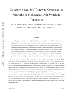
Figure 2.1 gives an example of a standard tree enterprise. Since (V,E) is a tree
there is, for every p G V, exactly one path p 0 = r , p 1, . . . , p t = p from the root
to p, such th a t {Pi ,Pi +1 } G E for all t, with the convention th a t the path consists
2
of r only if p = r . Define the predecessor of p G Vr\{ r} by n(p) := p t _i_. The edge
{ 7 r(p), p} is denoted by ep and the costs of this edge by cp , hence cp := c({n(p),p}).
For practical use we define cr := 0. Note th a t the m ap n and the set of nodes V
together determine the structure of the tree.
We define a partial ordering on the set of nodes V by:
p <q
the (unique) path from the root r to q contains p.
A trunk of (V, E) is a non-empty set of nodes T C V with the property: if p G T and
q < p then also q G T. In particular every tru n k contains the root r. Let p G V.
The branch o f p , B p , is the following subset of V: B p := { q G V | p < q).
For U C V define N ( U ) := {Jp€U N p , the set of players in U (we use this term
instead of ‘inhabitants’) and n(U) := \N(U)\, the number of players in U. Further let
N := N ( V ) and n := |iV|, the set and the num ber of players in the tree respectively.
If there is no node q G V such th a t n(q) = p then p is called a leaf. If, in addition,
n p = 1 then p is called a lonely leaf. (We write n p instead of n({p}). ) The costs of
an arb itrary subset U of nodes are defined by c(U) := ^2p€U cp and the costs of the
standard tree enterprise by c(F) := c(V). The problem we consider is how to share
c(F) among the players. This is in general not im mediately clear, as the edges are
used by different players.
Figure 2.1: Example of a standard tree enterprise. The numbers in the nodes denote
the numbers of inhabitants. Some nodes can be ordered w.r.t. <, e.g. r < p \ <
P 2 ^ Pb, but e.g. P 2 and p$ cannot be compared. The nodes P 4 , p$ and p g are
leaves and p?, is the only lonely leaf. The tree can also be described by the map n:
n( p4) = ir(p5) = P 2 ,7 t(P 6 ) = P 3 , t t ( P 2) = ?r(P 3 ) = Pi and n( pt ) = r. The set of
nodes T = { r , p i , p 2 , p 3 , p 5 } is an example of a trunk and B P2 = { p 2 , P 4 ,Pb} is the
branch of p^.
We only consider the following subset of standard tree enterprises:
T := {F | cp > 0 Vp
G
V, n (V ) > 1 and Vp
3
G
V : [n ( B p ) = 0
c(Bp ) = 0]}.
The subset of T with n players is denoted by T (n ). The set T contains standard
tree enterprises with non-negative costs, such th a t the costs of every branch without
players is 0. Note th a t em pty nodes are allowed and in particular em pty leaves. In
addition, it is allowed to have players in the root and to have more than one outgoing
edge of the root. Let p G V with n(p) = r. The standard tree enterprise with node
set B p U { r } is called a component of F. Usually we call elements of T ‘trees’ for short.
The set T is rather large. The reason th a t we have chosen such a large set is th a t
we stay in this set when we perform some operations on trees, like with ^-consistency
(see Section 3). The following subset of T contains trees with strictly positive costs
on the edges, no empty leaves and no ‘empty villages along the road’. In fact, this is
the class in which we are interested.
To := {F
G
T | Vp
G
Vr\{ r } : cp > 0 and [np = 0 =£- \{q
G
V | tt(q) = p}\ > 1]}.
A single valued solution rule on T is a m ap a which assigns to every F G T a
vector <r(F) in RN . The value <7j(F) denotes the am ount of money th a t player i has to
pay. The restriction of <r(F) to the players in iV\{*} is denoted by <7_,(F). Solution
rules for cost allocation on a fixed tree can be obtained by considering for every F G T
a corresponding cost game:
D e fin itio n 2.2: Let F := ((V , E ) , r , c , ( N p )pev ) G T . The corresponding standard
tree game is a pair (N, C ) where the cost function C : 2N
R is defined as follows:
C ( S ) is equal to the minimal to tal costs of the edges necessary to connect all members
of S with the root.
o
The proof of the following proposition can be found in G ranot et al. (1996).
P r o p o sitio n 2.1: Standard tree games are concave games.
A solution rule on standard tree games can be considered to be a solution rule
on T . This paper initially studies solution rules on standard tree enterprises apart
from standard tree games, although im portant relations will be mentioned. The next
section introduces a num ber of properties of solution rules on T . The last property,
^-consistency, is the most im portant one for this paper.
3
Properties of solution rules on trees
This section introduces properties of solution rules on trees. It will appear th a t the
properties are not logically independent. Let a be a single valued solution rule on T .
Let F := ((V, E ) , r , c , ( N p )p€V) G T .
Efficiency (E f f ) Efficiency means th a t the players pay together exactly the costs of
the edges: ' E i €N rTi(T ) = c(r ) = E p ev cv
Contraction ( Contr) Let p G Vr\{ r } such th a t cp = 0. C ontraction of edge ep
means identifying nodes p and ir(p). A solution rule satisfies Contraction if
every player has to pay the same am ount before and after the contraction. Note
th a t contraction of a zero-edge does not influence the related standard tree
game. Let us give an example:
4
Figure 3.1: Example of a contraction: edge eP2 has costs 0. Nodes p \ and P 2 are
contracted to a new node p r .
Deletion (Del) Let p G Vr\{ r} be an em pty village ‘along the road’, (i.e. n p = 0 and
|{<7 G V | 7r (q) = p ) | = 1). Let F' denote the tree obtained by deleting node p,
where the cost function c' is given by
c'q '■= c p + cq if 7T(q) = P and c'q := cq otherwise.
The solution rule a satisfies Deletion if ct(F) = a(T'). Again (N , C ) does not
change. Every game-theoretical solution rule satisfies Contraction and Deletion.
Figure 3.2 gives an example.
Figure 3.2: Deletion of the em pty node p%.
Homogeneity (Horn) A solution a is called Homogeneous if for every A > 0 we have
<r(F) = Act(F), where f := ( ( V , E ) , r , c , (Np )p e \z) and c (e ) := Ac(e) Ve G E. In
5
words, if the costs of all edges are multiplied by the same constant A > 0, then
all coordinates of <r(F) are multiplied by A.
Reasonableness (Reas) The stand alone costs of player i G N p are equal to sa,(F) :=
qfzpGg, where P is the path from the root r to node p. Note th a t sa,(F) =
C(i). The m arginal costs of i, m cj(F), are equal to mc,(F) = C ( N ) —C ( N \ { i } ) .
A solution rule a is called Reasonable if m c,(F) < <7, (F) < sa, (F) Vi G N . So
every player pays at least his marginal costs and at most his stand alone costs.
In particular <7, (F) = 0 if i G N r because sa, (F) = mc, (F) = 0 for such a player.
Milnor (1952) has studied reasonable outcomes for n-person games. Figure 3.3
gives an example.
Figure 3.3: I f i G N Pl then m c,(F) = 0 and sa,(F) = 10. I f i G N P2 then these
amounts are equal to 0 and 17 respectively. Finally if i G N P3 then mcj(F) =
3, sa,(F) = 13.
Fair ranking (F R ) Fair ranking says th a t players living closer to the root pay weakly
less than players who live farther away. More precisely, a satisfies Fair ranking
if
p < q.i (r Xp. j (r Xq
;■ o-j(F) < CTj(F).
In particular two players living in the same village pay the same (take q = p).
So Fair ranking implies ‘equal treatm ent of equals’.
Cost-monotonicity ( CostMon) This property says th a t players do not pay less, when
the costs of an edge are increased. Let p G Vr\{ r} such th a t n ( B p ) > 0.
Let F' := (V, E , r , c ' , (Np )p e v ) G T be the standard tree enterprise obtained byincreasing the costs of edge ep by 6 > 0, i.e. c'p := cp + 6 and c'q := cq otherwise.
A solution a satisfies Cost-monotonicity if <7,(r') > <7,(r) for all i G N .
Population-monotonicity (PopMon) This property has to do with the departure of
a player w ithout paying. Nobody pays less in the reduced situation. We have
to be careful with defining the reduced situation, because if e.g. the player who
leaves is a lonely leaf with positive marginal costs, then just deleting this player
from its village gives a tree which is not an element of T . If a player leaves then
6
the edges which are not used by the remaining players are no longer needed.
Therefore we do not only delete a player i from node p. but we also delete
the p art of the path from p to the root r which is used by player i only. In
other words, if the m arginal costs of player i are 0, then no edges are deleted,
otherwise the edges who determ ine the m arginal costs are deleted. In this way
the reduced tree F' is an element of T . For example if the player in p 6 of Figure
3.2 leaves then both edge ePe and eP3 are deleted. The solution rule a satisfies
Population-monotonicity if <7j(F) < <7j (F') for all i, j € N , where F' as described
above and n > 2.
v-Consistency (v-Cons) In the literature several notions of consistency on the class
of TU-games have been studied. The central idea is th a t a solution rule assigns
to a ‘reduced problem ’ with less players the restriction of the outcome of the
original problem. The question is how to define the ‘reduced problem ’. For trees
there are different possibilities. In this paper we study one of the possibilities.
Let n > 2, p € V, i € N p , x := <7j(F). Suppose th a t player i pays x and leaves.
In the reduced situation the remaining m aintenance costs c(F) —x have to be
shared among the other players. We want the reduced situation to be a tree in
T which differs from the original one only w.r.t. player i and the costs. To get
a tree with costs c(F) —x the am ount x has to be subtracted somewhere from
the costs of the edges. As i only uses the edges of the p ath P from p to the root
r it seems natural to subtract x from the costs of P; i pays only for edges he
uses. In the case of ^-consistency the costs are subtracted in the following way:
decrease the costs of the edges of the path P, starting in p and going towards
the root r. First the costs of the edge closest to the village where i lives are
decreased until x is subtracted or the costs have become 0. Then the costs of
the next edge on the path to the root are decreased and so on. Figure 3.4 gives
an example.
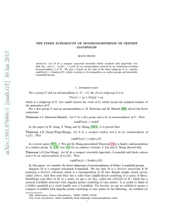
Figure 3.4: Example of ^-consistency: suppose th a t one of the players in p 2) say i,
leaves and th a t x := o f (F) = 9. Then we first subtract 7 from the costs of eP2, which
becomes 0. The remaining 2 are subtracted from the costs of edge ePl .
Subtracting costs in this way may cause problems, namely if x < mc, (F) or x >
sa,(F). Therefore we assume for v-Consistency th a t a satisfies Reasonableness.
7
The reduced standard tree enterprise with respect to player i is denoted by F* i
where x := <Tj(F). Reasonableness of a implies th a t F *j f T . A solution a
satisfies v-Consistency if V* € N: <7(F*j) = <7_j(F), where x := <7j(F). Note
th a t the reduced tree with respect to a player in the root is obtained by just
deleting this player. Let (N, C ) and (N , C) be the standard tree game associated
with F and F* i respectively. It is not difficult to show th a t
C(S) =
m in {C 7 (S ),
C( S
U { * } ) - æ j.
So the standard tree game associated with the reduced tree is exactly the
Davis-Maschler reduced game of the game associated with the original tree.
The term V-consistency’ is introduced in P otters and Sudhôlter (1995). The v
has been chosen because the nucleolus satisfies this kind of consistency. They
also study another kind of consistency on airport games, which they call i[iconsistency’ and which is satisfied by the ‘modified nucleolus’, introduced by
Sudhôlter (1997). In the case of [¿-consistency, costs are subtracted from the
path from the root to the node where a player lives, starting in the root. It can
be shown th a t there is no solution on T satisfying [¿-consistency, Reas and FR.
The properties we introduced are not logically independent. We have e.g.
P r o p o sitio n 3.1: Let a be a solution rule on T ­
a. I f a satisfies Reas and v-Cons then a also satisfies Eff.
b
I f a satisfies Contr, Reas, v-Cons and CostMon, then a also satisfies PopMon.
Proof:
a The proof is by induction to the num ber of players. Suppose th a t a satisfies Reas
and v-Cons. If n = 1 then c(F) is equal to the costs of the path from the root
r to the node where the player lives, i.e. c(F) = sai(F ) = m ci(F). By Reas we
have m ci(F) < <7i(F) < sai(F ). So <7i(F) = c(F) and efficiency follows.
Now suppose th a t a is efficient if the num ber of players is at most n — 1 (n > 2).
Take a tree F € T (n ). Choose a player, say i, and let x := <Tj(F). Applying vCons with respect to player i gives a tree F* t with n — 1 players. The induction
hypothesis together with v-Cons gives
E
jeN \i
CTi(r ) =
E
^•(r îi) = c(rîi) = c (r )- a: = c (r )- <7i(r),
jeN \i
from which it follows th a t a is efficient.
b
Suppose th a t a satisfies Contr, Reas, v-Cons and CostMon. Let T £ T , i £ N,
n > 2 . Player i and some edges, say E', are deleted giving a tree F '. Note th a t
E' = 0 if mcj(F) = 0. Applying v-Cons w.r.t. player i gives a tree F *j. Let
F" be the tree obtained by deleting E' from F*
Then CostMon, Contr and
v-Cons give th a t for all j G Ar\{ i} : <Tj(F') > <7y(F") = <7y(r*j) = <7y(F).
□
8
The next proposition says th a t a solution rule on T can be uniquely extended if
we know it for standard tree enterprises with 1 or 2 players and if it satisfies Reas,
v-Cons and CostMon. This is im portant for the characterization in Section 6.
P r o p o sitio n 3.2: Let a , r be two solution rules o n T . I f a and r both satisfy Reas,
v-Cons, CostMon and if a = t if n < 2, then a = r.
P roof: Suppose th a t a and r both satisfy Reas, v-Cons, CostMon, th a t a = t if
n < 2 and th a t a ^ r. Let F be a tree with a minimal number of players for which
a ^ t . Then n > 3.
Let i £ N such th a t <7j(F) > r, (F) (i exists because a and r satisfy E ff by Lemma
3.1). Then from v-Cons, CostMon and the definition of F we get
a-i(T) =
< a(TT_ l P ) = r ( r l f }) = r_ j(F ).
(3.1)
Now take a j £ Ar\{ i} . Again v-Cons and CostMon and the definition of F give
a - j (F) = a ( F ^ (r)) > a (F r_ f ^ = r ( F ^ r ) ) = r_ j(F ).
(3.2)
Next let k £
Then ct^F ) = ^ ( F ) by (3.1) and (3.2). So by v-Cons and the
definition of F we have (using x := ak( T) = Tk(T))
a _ fc(F) = a(T*_k) =
from which it follows th a t
ct(F)
t (T*_k)
= r - k (T),
= r(F ), a contradiction.
□
We now want to answer the question ‘Can we find solution rules satisfying the
properties of Section 3?’. We sta rt with a sub-question ‘Can we find solution rules
satisfying v-Cons?’. This is not immediately clear. The next section gives a oneparam eter family a a , a £ [0,1] of solution rules on T which all satisfy v-Cons.
In Section 5 we show th a t a a satisfies all properties introduced in Section 3 for all
a G [0,1],
4
D efinition of th e solution rules <ra
For every a £ [0,1] we define a solution rule on T . The com putation of a a consists of
com puting trunks with minimal ‘weights’. We sta rt - more general - with introducing
weights for connected parts of a tree.
4.1
Prelim inaries
Let a £ [0,1], F G T. We only compute weights in trees w ithout players in the root.
Therefore we assume in this subsection th a t N r = 0. Let Q C V be a nonemptyconnected set of nodes, Q ^ {r}. The degree of Q, d(Q), is the num ber of ‘outgoing’
edges of Q used by at least one player and not starting in the root:
d(Q) := |{p £ V \ Q | tr(p)
9
G
Q \ { r } , N ( B P) # 0}|.
The num ber i(Q) counts the ‘incoming’ edges of Q used by a t least one player and
not starting in the root. If Q U {r} is connected or Q is contained in a branch w ithout
players then i (Q) = 0; otherwise i ( Q) = 1. Consider for example the left tree of
Figure 3.1. For Q i = { p 2 , P 4 ,Pb} we have d(Qi) = 0, i(Qi) = 1. For Q2 = {P i , P 3 }
these numbers are 2 and 0 respectively. The grade of Q is defined by
ga(Q) : = n ( Q ) + a ( d ( Q ) - i ( Q ) ) Then g a (Q) > 0, because assuming th a t ga (Q) < 0 implies i (Q) = 1, d(Q) = 0
and n(Q) = 0 which is impossible (because n ( Q ) = d(Q) = 0 implies i(Q) = 0).
Note th a t, for Q i and Q 2 as defined above, we have g a (Q 1 U Q 2 ) = 8 + a ( l —0) =
4 + a(0 —1) + 4 + a (2 —0) = g a (Qi) + g a (Q 2 )- This property always holds if Qi U Q 2
is connected and Qi n Q 2 Q {t1}, because the number of players is additive and there
is at most one edge which connects Q 1 and Q 2 , which cancels.
The weight of Q is defined by
f jig iy
w a (Q) := < 00
[0
i f .?»(«) > 0
if g a (Q) = 0 and c(Q) > 0
if g (Q) = 0 and c(Q) = 0 .
We are in fact interested in pairs (c(Q),ga (Q)), but we use the function w a to order
the pairs in R+ U {00}. Therefore it is not allowed to simplify the fractions.
The following lemma will be used often in Section 5, in particular when Q2 is a
trunk:
L em m a 4.1: Let Q 1 and Q 2 be connected subsets o f V with QiC]Q 2 C {r} and such
that Q 1 U Q 2 is again connected. Then
w a (Q1) < w a (Q2) <=> w a (Q1) < w a (Q! U Q2) < w a (Q2)
and
w a (Qi) < w a (Q2) <=> w a (Q1) < w a (Q! U Q2) < w a (Q2).
Proof: The proof is straightforw ard and mainly based on the following relation:
m
,
rac'i
a+ c
rac'i
m
< ----- - < m a x < - , - >
lb d) ~ b + d ~
lb d)
b,d>0.
□
Now let T be a trunk. We have g a (T) = n (T ) + ad(T) > 0 and g a (T) = 0 implies
n(T ) = 0 and ad (T ) = 0. As there is at least one player outside the root, there is
always a tru n k for which ga (T) > 0, i.e. with finite weight. Therefore
w“(r) :=
min{wa (T) | T tru n k of T , T
10
^ {r}}
is finite. If a is fixed then we omit it in the notations.
Consider the tree in Figure 2.1. For a = 1 we have
_
10 17 20 22 21 24 26 22 25 27 26 29 31 13 15
15
and there is one trunk with minimal weight: T* = { r , p \ , p z , p o } .
4.2
D efin ition o f
cra
Let a G [0,1]. The idea of the solution rule a a is th a t villages closest to the central
supplier choose some neighbouring villages with which they want to cooperate. They
pay a part of the costs of the edges they use themselves and the remaining costs
are paid by villages further away. The value a determines which part of the costs is
‘shifted’.
We define the solution rule a a by an algorithm. The algorithm consists of com­
puting repeatedly the maximal (w.r.t. the num ber of nodes) tru n k Tm with minimal
weight wm(F). The players in Tm each have to pay wm(F). Then these players leave
and Tm is ‘contracted to the ro o t’. The costs of every outgoing edge of Tm, i.e. the
edges which d(Tm) counts, are increased by a w m (T). The following algorithm gives
the details. We use the fact th a t the function n determines the tree.
C o m p u ta tio n o f cra
Take F € T, a G [0,1].
S tep 1: P u t a f (F) := 0
Vi G N r and delete the players in the root.
S tep 2: Com pute wm(F) := min{w(T) | T tru n k of T , T ^ { r }} and let Tm be the
maximal tru n k with minimal weight.
S tep 3: P u t a f (F) := wm(F) for all i G N ( T m);
Com pute the tree where Tm is contracted:
V : r' U V \ 7 ,1,: N r, = 0;
p) := i r'
if Av) e Tm,
\ n(p) otherwise;
cP := cp + a w m (T) if n(p) G Tm\ { r } and N ( B p ) ± 0;
7r := 7r'; r := r':
N := N \ N ( T m);
S tep 4: R epeat Steps 2 and 3 until there are no players left.
The num ber of trunks is finite, so there is a trunk with minimal weight, but
there can be more than one tru n k with minimal weight. Lemma 4.2 shows th a t ‘the
maximal tru n k with minimal weight’ is a correct definition. In every iteration, the
num ber of remaining nodes strictly decreases, hence the algorithm stops after finitely
many iterations.
11
L em m a 4.2: Let a G [0,1] be fixed.
a I f Ti and T2 are both trunks with minimal weight, then the union Ti U T2 has also
minimal weight.
b I f T is a trunk with minimal weight and T = Ti UT2 with Ti C\T2 = {r }, then both
Ti and T2 have minimal weight.
P roof:
a Suppose th a t Ti and T2 are two trunks with minimal weight. The statem ent follows
immediately if Ti C T2 or T2 C Ti, so we suppose th a t this is not the case. The
proof consists of applying Lemma 4.1 a num ber of times. Let S := Ti fl T2. If
S = {r} then (in particular) w(Ti) < w(T2), hence w(Ti) < w(T\ UT2) < w(T2)
and it follows th a t Ti UT2 has also minimal weight. If S ^ {r} then w ( T i \ T 2) <
w(S) (because if w(S) < w (Ti \ T 2) then w(S) < w ( S U (T i\T 2)) = w(Ti) which
gives a contradiction because S is also a trunk). So w (Ti \ T 2) < w ((T i \ T 2) U
S) = w(Ti) = w (T2) and w(T±\T2) < w ((T i \ T 2) U T2) = w(T± U T2) < w(T2).
Therefore w(Ti U T2) = w(T2).
b Suppose th a t T is a trunk with minimal weight and T = Ti UT2 with Ti fiT2 = {r}.
If w (Ti) ^ w(T2) then by Lemma 4.1 m in{w(Ti), w(T2)} < w (T), contradicting
th a t T has minimal weight. So w(T\) = w(T2) and, again by Lemma 4.1,
w (Ti) = w (T) = w (T2).
□
R em ark: From b it follows th a t if there is more than one edge starting in the root,
then we can split the problem and compute a a for the components of F.
We shall now compute a a for the tree in Figure 2.1 for different values of a. We
sta rt with a = 1. We have already seen th a t T* = { r , p i , p s , p Q } is the unique tru n k
with minimal weight wm(F) = y-. So a f (F) = y- for all i G N(T*). C ontraction
of T* gives the left tree of Figure 4.1. Now we find th a t T* = { r , p 2 } is the unique
tru n k with minimal weight wm(F) = 3^-, hence the player in p 2 pays this amount.
C ontraction of T* gives the right tree of Figure 4.1. Now we find immediately th a t
a f (F) = 3 | j for the players in p 4 and a f (F) = 8 ^ for the player in p 5. We can
summarize this as ( 2 y ,3 ^ j-,2 y ,3 |j,8 ^ j- ,2 |), where the i-th coordinate is the am ount
th a t a player in node pi has to pay. In the same way we find for a = \ the am ounts
(2i| , 3 | f , 2 i| , 3 f , 6 ^ , 2 ^ ) and for a = 0 we find ( 2 | , 3 | , 2 | , 3 | , 5 ,2 f).
We defined solution rules a a for a G [0,1]. In the same way we can define solution
rules for a > 1. It will appear th a t such rules do not satisfy all properties introduced
in the previous section.
12
P4
3 ) ï*5
P4
©
r
Figure 4.1: Trees in the com putation of a 1 for the tree in Figure 2.1.
P roperties o f the solution rules <ra
5
This section studies two kinds of properties of the solution rules a a . Section 5.1
shows th a t a a satisfies the properties as introduced in Section 3. Section 5.2 studies
the relationship between the solution rules a a (a £ [0,1]) and well-known solution
concepts for (standard tree) games.
5.1
P rop erties o f solu tion rules
In the proofs we use several times two trees F and F'. The weights w.r.t. F (F') are
denoted by w (w ' ) and the maximal trunk with minimal weight is denoted by Tm
(T4). The costs and grades w.r.t. F (F') are denoted by c and g (c' and g').
P r o p o sitio n 5.1: The solution rule a a satisfies Ef f for all a £ [0,1].
P roof: E f f follows from the fact th a t the costs of every trunk Tm are paid
• partly by the players in Tm: „(Tj f f ”] (Tm) c(Tm),
• partly by shifting costs: n^ a)+ad(T )c(^m)-
□
P r o p o sitio n 5.2: The solution rule a a satisfies Contr for all a £ [0,1].
P roof: Let F £ T and let p £ Vr\{ r } such th a t cp = 0. If p is the only node besides
the root, then a a assigns 0 to all players before and after contraction. Otherwise let F'
be the tree after contraction of edge ep . There is a one-to-one correspondence between
trunks T ' in F' and trunks T in F with p £ T or n(p)
T such th a t corresponding
trunks have equal weights. If T is a trunk in F with it(p) £ T and p $ T , then
w (T U p ) < w (T) (use w(p) = 0 and apply Lemma 4.1). So to find a tru n k with
minimal weight in F, it is sufficient to consider only trunks with p £ T or it(p) T.
As a consequence we can contract in F and F' corresponding trunks Tm and T ^ and
wm(F) = «4 (r')13
If p £ Tm, the trees after contraction of Tm and T^ are the same and a a is the same
for the remaining players. If p $ Tm then n(p)
Tm and we have after contraction
of Tm a tree in which edge ep still has costs zero. Induction to the num ber of nodes
completes the proof.
□
P r o p o sitio n 5.3: The solution rule a a satisfies Del for all a £ [0,1].
Proof: Let F £ T and let p G Vr\{ r } such th a t n p = 0 and # { q G V | n(q) = p ) =
1. Let q be the unique node with n (q) = p and F' the tree obtained by deletion
of p. The proof is very similar to the proof of Contr. As a a satisfies Contr we
may assume th a t the costs on the edges are strictly positive. There is a one-to-one
correspondence between trunks T ' in F' and trunks T in F with q G T or p
T
such th a t corresponding trunks have the same weight. If T is a tru n k in F with
p G T and q $ T , then w (T \{p}) < w (T) because cp > 0. So to find a tru n k with
minimal weight in F, it is sufficient to consider only trunks with q G T or p £ T.
As a consequence we can contract in F and F' corresponding trunks Tm and T‘'m and
w m(F) = w'm(T').
If q G Tm, the trees after contraction of Tm and T ^ are the same and a a is the
same for the remaining players. If q Tm then p $ Tm and we have after contraction
of Tm a tree in which node p can be deleted. Induction to the num ber of nodes
completes the proof.
□
R em ark: as a a satisfies Contr and Del we assume from now on th a t T £ To- In
particular, costs on the edges are strictly positive and, as a consequence, weights of
trunks are strictly positive.
P r o p o sitio n 5.4: The solution rule a a satisfies Horn for all a £ [0,1].
P roof: If the costs of all edges are multiplied by the same A > 0, then all weights are
multiplied by A; and m ultiplication by A and taking the minimum can be interchanged,
because A is positive. So a a satisfies Horn.
□
P r o p o sitio n 5.5: The solution rule a a satisfies FR for all a £ [0,1].
Let p , q £ V, p < q. The rule u a divides the set of nodes V in groups, such
th a t <7° is constant for players in nodes in the same group. These groups correspond
with maximal trunks with minimal weights in subsequent iterations. If p and q are
in the same group, then FR immediately follows. For the other case, it is sufficient
to show th a t wm increases in subsequent iterations in the com putation of a a . This is
done in Lemma 5.6. In addition, the lemma shows th a t we can, in the com putation
of <7°, contract an arbitrary tru n k with minimal weight, instead of the maximal one,
w ithout changing the output of the algorithm.
L em m a 5.6: Let a £ [0,1] be fixed, T £%■ Let T* be a trunk of (V, E) with minimal
weight wm(F) =
and let T be an arbitrary trunk with T* c T . Let F' be the
tree after contraction of T* and let T ' := T \T * U {r'}. Then w '(T') > wm(F) and
equality holds if and only if w (T) = wm(F). A s a consequence w'm (T') > wm (T).
P roof: Let d := \{p £ T \ T * | n(p) £ T * \{r } }|, the number of edges in T which
14
costs are increased when T* is contracted. The following equalities hold:
• c'(T ') = c(T) - c(T*) + a w m (T)d,
• n '( T ') = n ( T ) - n ( T * ) ,
• d '(T ') = d(T) ^ d ( T * ) + d.
Using
Wm(r) < w(T) =
cm
(5.1)
we get
, , _ c(T) - c(T*) + a w m (T)d
W( } ~
g(T) - g(T*) + a d
>
~
=
wm(T)g(T) - wm (T)g(T*) + aw m(r)d
g(T ) - g(T*) + ad
wm(T).
(5.2)
Equality in (5.2) holds if and only if equality in (5.1) holds, i.e. if and only if
w(T) = wm(F). An arbitrary tru n k in F' can be seen as the result, after contraction
of T * , of a tru n k in F which contains T*. So w'(T') > wm(F) for all trunks T ' of F'.
Hence w'm(T') > wm(F).
□
P r o p o sitio n 5.7: The solution rule a a satisfies CostMon for all a G [0,1].
P roof: Let a G [0,1]. We use induction to the number of nodes. The case \V\ = 2
follows immediately. Take F G % with \V\ > 2. Let p G Vr\{ r} such th a t n ( B p ) > 0
and let 6 > 0. Let F' = (V, E, r, c', (Nq)qev) be the tree with cost function c'p := cp +6
and c'q := cq otherwise. We distinguish between two cases:
1. Suppose th a t there is a trunk T with w(T) = wm(F) and p T. Then w(T) <
w{TL) < w '( r4 ) < w'(T). Now p $ T implies w(T) = w'( T) hence w'(T) =
w '(T 4). So in both F and F' we can contract T. Then <7a (F) and a a (T') coincide
on N ( T ) and the shifted am ounts are equal (aw(T) = aw'( T) ). Hence, by­
induction, we have a a (T') > o-a (F).
2. Suppose th a t p G T for every trunk T with w(T) = wm(F). We increase the
costs of cp gradually. Define for every e > 0 the cost function c6 : V —¥ R+ by:
Cp := Cp + e and cq := cq otherwise. Let F e be the corresponding tree and let
be the maximal tru n k of Fe with minimal weight » ^ (F ). Define
:= m a x ji <
6 | there exists a trunk T with w(T) = wm(F), w l (T) = w ^F * )} . There exists
a tru n k Ti which has minimal weight with respect to both F and F 51. Then
wSl (Ti) > w(Ti) and in both cases contraction of Ti gives <jf (F51) > <jf (F) for
all i G N ( T i \ { r } ) . By induction we have <7a ( r 51) > o-a (F). We are done if
5 = S1. T i S 1 < S then let T* # Ti be such th a t w Sl (T*) = w Sl (Ti). If p $ T*
then we contract T* in F 51 and we are in case 1: we can increase cp arbitrarily.
If p G T' for all trunks T ' with w Sl ( T r) = w Sl (Ti) then we define d2 := m a x ji <
6 | there exists a tru n k T with w Sl(T) = w ^ (F ), w*(T) = w ^ F * )} . Now we
can repeat the procedure on F 51 and F 52. This procedure ends after finitely
many steps because the num ber of trunks is finite.
□
15
P r o p o s itio n 5.8: The solution rule a a satisfies Reas for all a £ [0,1].
P ro o f: Let T £ To, a £ [0,1]. If i £ N r then, clearly, Reas is satisfied. First the
marginal costs: take p £ V and i £ N p .
• If p is not a lonely leaf, then toc, (F) = 0 < a f (F) because weights of trunks are
nonnegative.
• If p is a lonely leaf then t o c , ( F ) = cp . If a trunk with minimal weight is
contracted, then nonnegative costs are shifted. So it is sufficient to show th a t
i pays at least his m arginal costs in a tree with p £ Tm. If Tm = { p , r } then i
pays cp . Now suppose th a t Tm ^ {p, r} and let T := Tm\{p}. If w(Tm) < cp
;
P
e (T )+ C p
n(T ) + l + a ( d ( T ) - l )
^
t h p n _______ C( T )_______ s ' r.
Cn
CP U l e U n ( T ) + a ( d ( T ) - l ) ^ CP ’ DU
W(T ) = ______ C(^) + CP_________
(
n(T ) + 1 + a(d( T) ^ 1)
______ C(^)_______ > W(T)
n ( T ) + a(d( T) - 1) 1 >
contradicting the fact th a t Tm has minimal weight. So o f (F) = w(Tm) > cp .
The proof for the stand alone costs is by induction to the number of nodes. The
case \V\ = 2 follows immediately. Now suppose \V\ > 2. We first show th a t a f (F) <
sa,(F) for all i £ N ( T m). Let p £ Tm\ { r } ,i £ N p . Let P be the unique path from p
towards the root r. As P is also a trunk we have
o'“ (F) = w(Tm) < w(P)
rU^ < c(P) = sa,(F).
g(P)
(5.3)
Let i N ( T m) and let F' be the tree after contraction of Tm. It is sufficient to show
th a t sa,(F) > sa,(F ') (induction completes the proof). To prove this inequality let q
be the first node in Tm on the path from p to r (in F). It is sufficient to show th a t
a w ( T m) < c(P) where P is the p ath from the root r to node q. The inequality follows
immediately if a = 0 and if a > 0 then g(P) > 0 and we can apply Formula (5.3). □
P r o p o s itio n 5.9: The solution rule a a satisfies v-Cons for all a £ [0,1]
Let F £ To, p £ V, i £ N p and define x := a f (F). Let F* i be the reduced standard
tree enterprise, i.e. i is removed and the costs of the path from p to the root r are
diminished with x, starting in p (see also the definition of v-Cons). We have to show
th a t <7a (r * j) = <7“ j(F). This trivially holds if i £ N r , so we assume th a t p ^ r. In
addition we assume th a t N r = 0 (otherwise first apply v-Cons w.r.t. the players in
the root), th a t there is exactly one node q such th a t n(q) = r (w.l.o.g. by Lemma 4.2)
and th a t n > 2 . Let w be the weight with respect to F* i , w m the minimal weight and
let T m be the maximal tru n k with minimal weight w.r.t. F* We write w m instead
of wm(F).
We first consider the case p £ Tm and g(Tm) = 1. Then a = 0 and Tm is a path,
which costs are entirely paid by i. Then v-Cons with respect to player i followed
by Contr applied on Tm is exactly one iteration in the algorithm to compute a a (T),
hence ^ “ ¿(r) = <7a (r* j).
16
The proof of the case g(Tm) > 1 consists of a num ber of steps. We first show th a t
the weight of the minimal trunk does not change: w m = wm. We finish the proof th a t
cra satisfies v-Cons by induction to the num ber of nodes.
L e m m a 5.10: w m < wm .
P ro o f: We distinguish between some cases:
• Suppose th a t p £ Tm. Then we have w(Tm) =
we have w(Tm) = w(Tm) = wm. Therefore w m < wm.
As w(Tm) =
= x,
• Suppose th a t p $ T m and g(P) > 1, where P is the path from p to Tm.
— If x < c(P) then w m < w(Tm) = w(Tm) = wm.
- If x > c(P) then uJm < w(Tm UP) = g(r” )+g(p)Ii < fofel = W(T™) =
• Suppose th a t p $ Tm and g(P) < 1 i.e. n(P ) + a(d(P ) — 1) < 1, which is onlypossible if d(P) = 0,n (P ) = 1 and a > 0 (because i £ N ( P ) , so n(P ) > 1).
Then P = {p} and N p = {*} because we have assumed th a t there are no
em pty leaves and no em pty villages along the road. After contraction of Tm in
F the costs of edge ep are increased by a w m and we have x = aw (T m) + c(P).
Therefore wm < w(Tm) =
= w(Tm) = wm. (Note th a t there is no
division by zero, because if g(Tm) = a , then n(T m) = 0 and d(Tm) = 1. This is
impossible, since n(p) would be an em pty village along the road.)
□
Let S := Tm fi T m ^ {r}. We write T m = S U Q i U . . . U Qt . The sets Qt are
pairwise disjoint and each of them contains exactly one node qt such th a t 7r(qt ) £ S.
L e m m a 5.11: The following inequalities hold
w (Q t ) < w ( T m) < w(Tm) < w (Qt ).
P ro o f: Suppose th a t w (Q t ) > w ( T m). Then w ( Q t ) > w ( T m\ Q t ), because if w(Qt ) <
w ( T m\ Q t ) then w ( Qt ) < w ( T m) by Lemma 4.1. Applying Lemma 4.1 again gives
w ( T m\ Q t ) < w ( T m), which contradicts the definition of T m. The second inequality
is exactly the previous lemma. Now suppose th a t w (Q t ) < w(Tm). Then Tm U Qt is
a b etter candidate for Tm because w(Tm U Qt ) < w(Tm) by Lemma 4.1.
□
L e m m a 5.12: We have £ < 1 and if 1 = 1 then p £ Q 1 =: Q.
P roof: If p £ Tm we find w(Qt ) = w (Q t ) and therefore (by Lemma 5.11) £ = 0. If
p $ Tm, then there is at most one index t with Qt n P ^ 0, where P is the path from p
to Tm. Therefore £ < 1. Let us suppose th a t £ = 1 and th a t p $ Q. Let P denote the
path from p to Q. Note th a t x > c(P) (otherwise w (Q t ) = w (Q t j). So w(P) = 0 and
T m U P is a better candidate for T m for the tru n k is larger and w ( T m U P ) < w ( T m)
by Lemma 4.1.
□
17
We continue by distinguishing between some cases with respect to g(Q). Lemma
5.13 considers three cases which can all occur. Initially the cases of Lemma 5.14
cannot be excluded, bu t they all give a contradiction.
L em m a 5.13:
1. I f £ = 0 then wm = wm .
2. I f £ = 1 and g(Q) < 1 then wm = wm .
3. I f £ = 1, a = 0 and n(Q) = 1 (i.e. g(Q) = 1) then wm = w m.
P roof:
1. In this case T m C Tm.
• If p G T m then p G Tm and x = wm; therefore we have
—
c(T m) x _ c( Tm) wm
g ( T m)wm wm _
Wm ~ g ( T m) - 1 “ g ( T m) - 1 "
g ( T m) - 1
“
• If p T m then let P denote the path from p to T m. In this case x < c(P)
(because if x > c(P) then w(P) = 0 and T m U P is a better candidate for
T m by Lemma 4.1). So w m = w ( T m) = w ( T m) > w (Tm) = wm.
2. Note th a t g(Q) < 1
d(Q) = 0 , a > 0 and n(Q) = 1. So if g(Q) < 1 then
Q = {p} and P is a lonely leaf. Then x = cp + a w m and
_
wm =
c(S) + c(Q) — x
c(S) — a w m
g (T m)=——1 TcFs------------------------------------^
g(S) - a
-----------i —
g(S)w m — a w m
g(S) - a
3. In this case Q is a path. By Reas in the tree obtained by contraction of Tm we
have x < c(Q). Hence wm < w(S) =
□
L em m a 5.14: The remaining cases all give a contradiction:
1. n(Q) = 2,d(Q) = 0 and a = 1, (i.e. g(Q) = 1)
2. n(Q) = 1,d(Q) = 1 and a > 0, (i.e. g(Q) = I)
3. g(Q) > 1.
P roof: 1. First note th a t if n(Q) = 2,d(Q) = 0 and a = 1 then Q = {p,ir(p) =: q}
because the other three possibilities for Q give a contradiction immediately:
• Q = {p}- Then x > c(Q) otherwise S' is a better candidate for T m. Further
c(Q)+wm = x
implies w(Q) = c(Q) < wm and Tm U Q is a better
candidate for Tm.
18
• Q = {P-,q} with 7t(q) = P■ Now S U {p} is a better candidate for T m because
cq > 0.
• Q = {P)Q)Q}(7r(Q) = tt(p) = <?)• As cq > 0 we find th a t S U {p, q} is a better
candidate for T m.
C ontracting Tm in F and computing a a in the component which contains p gives
x = cp + 7j(cq + wm). As .)■ > c(Q) (because otherwise S' is a better candidate for T m)
we have eq < wm, which implies w({q}) < wm and Tm U {q} is a better candidate for
Tm. Contradiction.
2/3. We prove 2 and 3 partly simultaneously. We first show, by induction to
the num ber of nodes, th a t wm = w m. The case \V\ = 2 follows immediately. Let
F € To, i € N , be a counterexample with \V\ as small as possible. Let p be such th a t
i £ N p . Let F be the tree obtained by performing one iteration in the com putation
of <7a (r ) such th a t Tm is contracted. Let F 1 be the com ponent of F containing p.
Then F has less nodes than F and <jf (F) = x. Let
be the largest trunk of F 1
with minimal weight
We have w m <
(Lemma 5.6). We shall show th a t
w := wm((F1)*j) < wJjj which gives a tree with less nodes than F for which the
minimal weight strictly decreases when i leaves.
2. Suppose th a t n(Q) = 1,d(Q) = 1 and a > 0. In this case there are two
possibilities: Q = {p} or Q = {p, ir(p)}. In both cases we have x > c(Q), because
otherwise S' is a better candidate for T m. Now we get a contradiction:
W <
c(Q) + a w m - x
a
1
----------- < W m < W m .
3. Now suppose th a t g(Q) > 1. Using c(S) > g (S )w m and wm = g [s)+ g @ -i we
find c(Q) - x < w m (g(Q) - 1) < wm(g(Q) - 1). So
c(Q) + a w m - x
W < ------T= T ------ — --------- < W m < W m .
g(Q) - 1 + a
Conclusion: in all cases w m = wm- We shall now show th a t Tm U T ^ \{ f} is a
better candidate for Tm, from which it follows th a t the last two cases of this lemma
can not occur.
2. If n(Q) = 1, d(Q) = 1 and a > 0 then we have
w(Tm)
=
-
r r i\
Wm ( F
) = W <
c(Q ) + a w m - i
-------------------------------- < W m < W
i\
(Tm)
=
c (f^ ) + aw m
where the last inequality follows from FR. Now we find w (T^) = g^ r^ a = wm and
by Lemma 4.1: w(Tm U T ^ \{ f} ) < w(Tm).
3. Finally if g(Q) > 1 then we find:
r r i\
W (T J = Wm(F ) =
W
c{Q) + a w m - x
.
< -----=----- —------ < Wm < w(Tm)
g( Q ) - l + a
19
and again Tm U T ^ \{ f} is a better candidate for Tm.
□
Now we can finish the proof th a t a a satisfies v-Cons by induction to the number
of nodes. If \V\ = 2 then v-Cons follows immediately. Now suppose th a t \V\ > 2.
From Lemma 5.13 (and 5.14) we learn th a t w m = wm. If we go through the proof of
Lemma 5.10 we see th a t w(Tm) = w ( T m), i.e. Tm has minimal weight with respect to
w and therefore Tm C T m. We distinguish between the same cases as in Lemma 5.13:
•
If £ = 0 then Tm = T m and
uJm =
wm so
(F)
=
<7“ (F* t) for all j
G
N ( T m).
If p G Tm then we find after one iteration in the algorithm the same tree for
F and F *j. So we also have u f ( T ) = <t“ (F*j) if j
N ( T m). If p $ Tm then
x < c(P) and one iteration in the algorithm applied on F and F* t respectively
gives again a tree F 1 and its reduced tree (F1) ^ . We can proceed by induction.
• If £ = 1 and g(Q) < 1 then T m = Tm U {p} and N p = {i } , d ( Q ) = 0 , a > 0.
C ontraction of Tm gives a tree F for which {p, r } is a trunk. We first contract
{p, r }. Then we get the same tree as the one obtained by applying one iteration
of the algorithm on F* i , such th a t T m is contracted.
• l i £ = \ , a = Q and n(Q) = 1 then T m = Tm U Q and Q is a path. One iteration
in the algorithm applied on F and T* such th a t in both cases Tm is contracted,
gives a tree F 1 and its reduced tree (F1)** and induction completes the proof.
5.2
G am e-th eoretical properties
The first question we ask is whether there is an a G [0,1] such th a t a a is equal to
well-known solution concepts for standard tree games. The answer is affirmative in
case of the nucleolus and the constrained egalitarian solution as Theorem 5.15 shows:
T h e o r e m 5.15:
• I f a = 1 then a a coincides with the nucleolus (Meggido (1978)).
• I f a = 0 then a a coincides with the constrained egalitarian solution (Dutta and
Ray (1989)).
For the Shapley value (Shapley (1953)) and the r-value (Tijs (1981)) we get nega­
tive answers, because both solution concepts do not satisfy v-Cons as the following
example shows:
E x a m p le 5.1: Consider the standard tree enterprise F as indicated in Figure 5.1.
The Shapley value of the standard tree game (N, C ) related to F is given by
$¿((7) = y + ^ = 9 | i f i G N q , $¿((7) = y = 2 | if * G N p . Reduction with respect
to a player in node q gives the tree F. Now we have $¿((7) = ^ ^ <£*(C') if i G N p .
The r-value of (N , C ) becomes r,((7) = 9 if i G N q and r,((7) = 3 if i G N p .
Reduction with respect to a player in node q yields the tree F'. Then r, (C") = 4 ^ ^
Tj (C) if i G Np.
o
20
20
(I) P
10
11
10
-LUg
­
CD P
10
0
p
10
Figure 5.1: Standard tree enterprises F, F and F' respectively.
The next proposition shows th a t a a is a core element of the related standard tree
game for all a £ [0,1].
P r o p o sitio n 5.16: Let a be a solution rule on T satisfying Reas and v-Cons. Then
Corel .Y. C) := {y G R ^ | y ( N ) = C (N ), y(S) < C (S) V S C N } for all
c t(F ) g
F G r.
P roof: The proof is by induction to the num ber of players. If n = 1 then <r(F) =
c(P) = C (N ), where P is the path from the root r to the node the player lives in.
Let F g T with n > 1, x := <t(F), i £ N . Let (N , C ) be the game related to F ^.
i.e. N = i V \ { i } , C ( S ) = m in{C'(S'U { ¿ }) —X i , C ( S ) } VS C N. By v-Cons with
respect to player i and the induction hypothesis we get
<7_j(r) = f ^ r ^ )
G
Corel .Y. C).
So x ( N ) = C ( N ) and x (S ) < C ( S ) for all S C N . From x* > me, = C (N ) — C ( N )
and x ( N ) = C (N ) it follows th a t x ( N ) = C (N ) + X i = min{(7(iV) —x*, C (N )} + X i =
C (N ).
_
Now let S C N . If * G S then x ( S \ i ) < C ( S \ i ) < C (S) — x , and therefore
x(S ) < C(S). H i ^ S then x (S ) < C (S ) < C(S). So x £ Corel Y .C).
□
6
C haracterization of th e solution rules cra
We shall now prove the main theorem of this paper.
T h e o r e m 6.1: Let a be a solution rule on T- Then a satisfies Horn, Reas, Del,
Contr, FR, CostMon and v-Cons if and only if there exists a parameter a £ [0,1]
such that a = a a .
We have already shown in the previous section th a t a a satisfies the seven prop­
erties. We shall now prove the ‘only if’ part. Suppose th a t a satisfies the seven
properties. Note th a t a also satisfies E f f by Proposition 3.1. We have, according to
Proposition 3.2, only to consider the cases n = 1 and n = 2. The case n = 1 follows
21
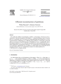
from Reas. Now let F G T , n = 2, say N =
It is sufficient to consider the four
classes of trees as indicated in Figure 6.1: T(2 , equal), T ( 2, separated), T(2, airport)
with cp > 0 and T (2, empty) with cp ,cq, cs > 0.
NP = {i,j}
T (2, equal)
©
N p = {*}
Q ) N q = {j }
T (2, airport)
Figure 6.1: Trees with two players.
On T (2,equal) we have <7j(F) = <7j(F) = cp / 2 = o f (F) = <t“ (F) for all a G [0,1]
by E ff and FR. On T ( 2 ,separated) we have, by Reas, <7j(F) = cp = <7f(F) and
<7j(r) = cq = <t“ (F) for all a G [0,1]. The next two subsections consider the other
two cases.
6.1
7~(2, airport)
This case is much more complicated. By Horn we may assume th a t cp = 1. Now <7,
and (7j are functions of x := cq. Consider the following function ƒ : R+
R, f ( x ) :=
Oi(T(x)), where T(x) as in Figure 6.2. So f ( x ) is the am ount th a t player i pays if
cp = 1 and cq = x. Then player i pays x + 1 — f ( x ) by E f f . For the <ra -rules, ƒ “
becomes: f a (x) = x + 1 — m i n j j ^ , =^1^} = m a x j ^ j i + 1,
So we want to
show th a t f ( x ) = m a x jl + f i x , for some ¡3 G [0, |] .
The seven properties of a put some restrictions on ƒ. We mention
• ^ ( x + 1) < f ( x )
Va; G R +
We write U := {x
G R+
• 1 < f ( x ) < 1 + \ x Vx
G
(FR).
| f ( x ) = ^ (x + 1)},
R + , in particular ƒ (0) = 1.
The first inequality follows from Reas. For the second one consider the tree F of
T (2, airport) in Figure 6.1 where cp := 0 and cq := x. In this tree both players
22
pay \ x by Contr, Ef f and FR. By CostMon we find x + 1 — f ( x ) > \ x , i.e.
f ( x ) < 1 + \ x . If f ( x ) = 1 + \ x on R+ then ƒ = ƒ “ for a = 1 and we are done.
So we assume from now on th a t f ( x ) < 1 + \ x for some
Let V : = { i e l ( . | f ( x ) = 1 + \ x } . Note th a t 0
• The function x 1—>■
G
V and U fi V = 0.
1 (x > 0) is (weakly) increasing.
Let x > 0, y > 1 and consider the tree F of T (2, airport) of Figure 6.1 where
cp := y, cq := x. By CostMon and Horn we find y ( | + 1
> * + 1 —f ( x ) ,
as was to be shown.
Suppose th a t f ( x i) = f ( x 2), where 0 < x \ < x 2- Then
1 <
1,
which implies f ( x i) = f ( x 2 ) = 1. As f ( x 2 ) > \ { x 2 + 1) we have x 2 < 1. In
particular ƒ is strictly monotonic on [l,oo).
• For every 6 > 0 : f ( x + (5) — f ( x ) < 6 Vx G R+ ( CostMon) and continuity of
ƒ follows. Note th a t V ^ R+, /( x ) > |( x + 1) and continuity of ƒ imply th a t
there exists a num ber x G R+ \ I / such th a t f ( x ) > 1. We use this later on.
a( x , y) ( T ) N p = {*}
1
f(x)
® i V p = {i}
b(x,y) (t ) N q = {j }
x + 1 - f(x)(Y) Nq = { j }
c ( x , y ) Q ) N s = {k}
X
X
© r
© r
Figure 6.2: The trees F(x) and T (x, y).
The property v-Cons with respect to i and j does not give extra conditions on
ƒ. We get new conditions if we consider the airport problem T ( x, y ) with 3 players
(Figure 6.2). Define the functions a, b, c :
—¥ R by: a( x, y) := Oi (T(x,y)),b(x, y) :=
Oj (T (x ,y) ) ,c (x, y) := Ok(T(x,y)). The conditions on a put conditions on a, b,c and
ƒ. For all (x, y) G R^_ we have
• a(x, y) + b(x, y) + c(x, y) = x + y + 1
• 1 < a(x, y) < x + y + 1
0 < b(x, y) < x + y
0 < c(x, y) < x.
(Reas)
23
(Eff ).
• 0 < c(x,y) < b(x,y) < a( x, y)
(F R ).
• Let 8 > 0. By CostMon: a( x, y) < a(x + 6,y + 6) and the same inequality holds
for b and c. By Eff: a(x + 6,y + 6) — a(x, y) + b(x + 6,y + 6) — b(x, y) + c(x +
6,y + 6) — c(x, y) = 28. So a(x + 6, y + 6) — a(x, y) < 28 and a is continuous.
Similarly b and c are continuous.
The conditions concerning v-Cons are more complicated:
• v-Cons(c) (i.e. v-Cons w.r.t. player k ) (Del):
a( x, y) = f ( x + y - c(x,y)).
(6.1)
• v-Cons(b):
— if b(x,y) < y then (Horn, Del)
T
(l + y - b ( x , y ) ) f ( — ------ --------) = a(x, y),
1+y-b{x,y)
(6.2)
— if b(x,y) > y then ( Contr)
a( x, y) = f ( x + y - b ( x , y ) ) .
(6.3)
• v-Cons (a):
— if a( x, y) < 1 + y then (Horn, Contr)
T
(1 + y - a ( x , y ) ) f ( — -------- ----- -) = b(x,y).
1+y-a{x,y)
(6.4)
— if a( x, y) > l + y then (Contr)
b(x,y) = c(x,y).
(6.5)
From now on, we only consider points (x, y) G
with y = x + 1 —f ( x ) . Therefore
we write a(x) instead of a(x, y) etc.
As f ( x ) > ƒ(0) = 1 for all x G R+, we have U C [l,oo). The following lemma
shows th a t U is an unbounded interval.
L e m m a 6.2: There exists a number u 0 > 1 such that U = [uq, og).
P ro o f: Take a: G K + \V such th a t f ( x ) > 1. Let y := x + 1 —f( x) and s := x + y —c(x).
From v-Cons(c) and E f f we get the following equalities:
a(x)
b(x)
c(x)
=
=
=
f(s),
s + 1 —f ( s ),
x + y — s.
We shall first show th a t s = x. From
s + 1 —ƒ (s) = b(x) > c(x) = 2ar + 1 —f ( x ) — s
24
we get s > x (FR and monotonicity of the function t
2t + 1 — f (t )) . Then
b(x) = s + 1 —f ( s ) > x + 1 —f ( x ) = y. So (by v-Cons(b) and v-Cons(c)) f ( x + y —
b(xj) = a(x) = f ( x + y —c(x)). If s > x then b(x) > c(x) which implies th a t a(x) = 1,
because ƒ is strictly monotonic on [1, oo). As a consequence f ( x ) < ƒ (s) = a(x) = 1,
contradicting f ( x ) > 1. Conclusion: s = x.
We further have a(x) < y + 1 (because if a(x) > y + 1, then f ( x ) = f ( s ) = a(x) >
y + 1 = x + 2 — f ( x ) gives 2f ( x ) > x + 2, i.e. x € V). Hence v-Cons(a) gives
(1 + y - a ( x ) )f (t (x ) ) = b(x), where t(x) := 1+yl a(x) = 2+a- 2f(x) - So
= x
+ 2
- 2f( x) =
+
Le'
^
€
U‘
So for x
V, f ( x ) > 1, we have t(x) G U. If x € U then t(x) = x and if x
U
then t(x) > x. Let uq be the smallest num ber in U (exists because U is nonempty,
closed and U C [l,oo)). Suppose th a t there exists a num ber x \ such th a t x \ > uq
and x \
U. We may assume th a t V fl (uq, x \) = 0, because one can always choose
x \ G («o, Vo), where vq := inf(Vr n [«o, oo)). Let x 2 be the largest num ber in U smaller
th an x \ . As x 2 € U we have i(x 2) = x2. If x2 < z < x i then z V, f ( z ) > |( z + 1) >
\ { uq + 1) > 1, so t(z) is well defined, t(z) G U and t(z) > z. B ut (x2,x i) fl U = 0
from which we get t(z) > X\ for all z € (x2,x i) . So i(x 2) > X\ (by continuity of t)
contradicting x 2 < x \ .
□
C o ro lla ry 6.3:
a) V = {0}.
b) I f ƒ is not strictly monotonic, then f ( x ) = m a x jl, ^ ( x + 1)} = f a (x) for a = 0.
P ro o f: a) Suppose v G F \{ 0 } . Take x > v, x > u q . Then | =
, i.e.
x e v n u = 0.
b)
Suppose th a t 0 < x\ < x 2 and f ( x i) = / ( x 2). We have already seen th a t
this implies f ( x i) = / ( x 2) = 1 and x 2 < 1. Let x := max{z G R+ | f ( z ) = 1}.
We follow more or less the proof of Lemma 6.2. Consider the point (x,y) where
y := x + 1 — f ( x ) = x and let s := x + y — c(x). Again, we have s > x (FR) and
b(x,y) > y (CostMon). Now v- Con s(6) gives a(x, y) = f ( x + y —b(x)) = f ( 2 x —b(x)).
From b(x) > y = x it follows th a t 2x — b(x) < x, so a(x) = ƒ (2x — b(xj) = 1.
Applying v-Cons(c) gives 1 = a(x) = ƒ (2x — c(xj), from which we get 2x — c(x) < x,
i.e. c(x) > x. This together with Reas gives c(x) = x and b(x) = x (E f f ). Finally,
a(xs) = 1 < 1 + y, so u-Cons (a) gives x f ( ' f ) = b(x) = x, i.e. / ( I ) = 1. Hence x = 1
and also uq = 1.
□
L e m m a 6.4: I f ƒ is strictly monotonic then for all x
G
(0, uq)
f ( x ) ^ 1 = f ( u o) - 1 =X
Uq
Note that ƒ is completely determined and 0 < (i <
P ro o f: Let x G (0 ,« o). Then /(^ 1 < ii'u^ 1 ■ Consider the point ( x,y) :=
(x, x + 1 —f ( x j). As f ( x ) > ƒ(0) = 1 and x
V, we get from the proof of Lemma
25
6.2 th a t a(x) < 1 + y and b(x) = y. Applying v-Cons(a) and v-Cons(b) gives
(1 + y — a (x ))f(t(x )) = b(x)
As t(x)
G
X
and
a(x) = f ( x ) , where t(x) := -----------1 y Qiixj
U (see again the proof of Lemma 6.2) we have
f ( x ) - 1 = f ( t ( x ) ) - 1 > ƒ (Up) - 1
X
t(x)
~
«0
So
f ( x ) - 1 = f ( u o) - 1
X
Uq
□
6.2
7”(2, em p ty)
We first consider the class T (3, nonem pty), consisting of trees like in T (2, empty) (see
Figure 6.1), but now there is one player in node s, say N s = {fc} and cs = 1, cp , cq > 0.
According to the previous section, there exists a num ber a G [0,1] such th a t a = o a
on T (2 ,airp o rt).
L em m a 6.5: On T (3 ,nonem pty), a = o a .
P roof: Take F G T (3, nonempty) and define x := cp , y := cq, a ( x , y ) := <7,(F),
b(x,y) := <Tj(r) and c(x,y) := a k (F).
From Reas we get a ( x , y ) > x and therefore applying v-Cons(a) and Horn gives
b(x,y) = y - f a {x+1^ y <
':X}V)). Similarly (v-Cons(b) and Horn) a(x, y)=x- f a ( y+1^ ( x,y) ^
As f a (z) = m a x jjq ^ z + 1, ^jp-}, the following equalities m ust hold:
i
a{x,y)
i/
\
b(x,y)
\
=
r a
t , i
u
w ,
x + y + 1 ^ b(x,y)
max{y-j—^ ( y + 1 —b(x,y)) + x , -------------------------}
=
r a /
/
w
x + y + 1 - a(x,y),
m ax{——- (x + 1 —a(x, y)) + y , -------------------------}.
1+ a
2
By distinguishing between four cases, in fact corresponding with four trunks of F,
it can be shown th a t a (x ,y ) = o f (F), b(x,y) = crf(T) and c(x,y) = crf(T).
□
L em m a 6.6: On T (2, em pty), o = o a .
Proof: Let F G T (2, empty). Define x := cp , y := cq. We may assume th a t cs = 1
(Horn). We construct a tree F' G T (3,nonem pty) with costs cp = x 1, cq = y 1 and
cs = 1, where x' and y' are defined later. Then we show th a t ct(F) = <7a (F) using
v-Cons(c).
We distinguish four cases, again corresponding with four trunks of F.
26
In this case o f (F) = \ + x,
j q T h e n we have
a fc(F') = a fca (F') = min{
(F) = | + y. Define
1
1 + 2a 2 —n
2 —n
o
1 + 2i i
Then ct^F') =
+ x',aj(T') =
+ y ' . Applying v-Cons(c) gives a
tree F" G T ( 2 ,empty) and <7,(F") = <7j(F'),<7j(F") = <7y(F'). By Horn we
have <7j(F) = 1j^2ag;(F ") = 1j^2ag;(F ') = x + | = erf (F). And similarly
(r ) =
( n
=
( n
= y + 1 =
(f).
For the next three cases we only give x' and y ' . The proofs are similar.
3+ x+ y'
□
References
[1] D a v is and M . M aschler (1965) The kernel of a cooperative game. Naval
Research Logistics Q uarterly 12, 223-259.
[2] D u b ey , P. (1982) The Shapley value as aircraft landing fees - revisited. M an­
agement Science 28, 869-874.
[3] D u tta , B . and D . R ay (1989) A Concept of Egalitarianism under Participa­
tion Constraints. Econom etrica 3, 615-635.
[4] G alil, Z. (1980) Applications of efficient mergeable heaps for optimization prob­
lems on trees. A cta Inform atica 13, 53-58.
[5] G ran ot, D ., M . M asch ler, G . O w en and W . Zhu (1996) The Ker ­
nel/Nucleolus of a Standard Tree Game. International journal of game theory25, 219-244.
[6] L ittlech ild , S .C . (1974) A Simple Expression for the Nucleolus in a Special
Case. International journal of game theory 3, 21-29.
[7] L ittlech ild , S .C . and G .F . T h o m p so n (1977) Aircraft landing fees: a game
theory approach. Bell Journal of Economics 8, 186-204.
[8] M aschler M ., J. A . M . P o tte r s and J. H . R eijn ierse (1995) Monotonicity
properties of the nucleolus of standard tree games. R eport 9556, University of
Nijmegen, The Netherlands.
27
[9] M eg id d o , N . (1978) Computational complexity of the game theory approach to
cost allocation for a tree. M athem atics of O perations Research 3, 189-196.
[10] M iln or, J .W . (1952) Reasonable outcomes for n-person games. The R and Cor­
poration 196.
[11] P o tte r s, J .A .M . and P. S u d h olter (1 9 9 9 ). Airport Problems and Consistent
Allocation Rules. Forthcoming in M athem atical Social Sciences.
[12] Shapley, L.S. (1953) A value for N-person games. C ontributions to the theory
of games II, H.W. Kuhn and A.W. Tucker eds. Princeton: Princeton University
Press, 307-317
[13] S on m ez, T . (1994) Population monotonicity of the nucleolus on a class of
public good problems. Mimeo University of Rochester
[14] S u d h olter P. (1 9 9 7 ). The modified nucleolus: properties and axiomatizations.
International journal of game theory 26, 147-182.
[15] T ijs, S .H . (1981) Bounds for the core of a game and the r-value Game Theory
and M athem atical Economics, eds. O. Moeschlin and D. Pallaschke, Amsterdam,
N orth Holland, 123-132
28