1. Art and Diseño

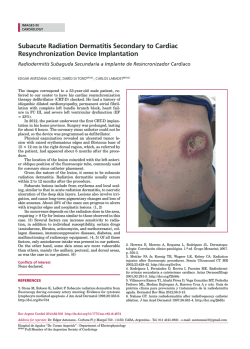
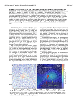
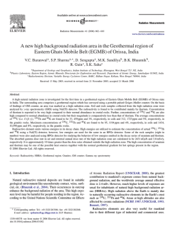
Hydrol. Earth Syst. Sci., 19, 601–613, 2015
www.hydrol-earth-syst-sci.net/19/601/2015/
doi:10.5194/hess-19-601-2015
© Author(s) 2015. CC Attribution 3.0 License.
Estimates of global dew collection potential on artificial surfaces
H. Vuollekoski1 , M. Vogt1,2 , V. A. Sinclair1 , J. Duplissy1 , H. Järvinen1 , E.-M. Kyrö1 , R. Makkonen1 , T. Petäjä1 ,
N. L. Prisle1 , P. Räisänen3 , M. Sipilä1 , J. Ylhäisi1 , and M. Kulmala1
1 University
of Helsinki, Department of Physics, Helsinki, Finland
Institute for Air Research, Oslo, Norway
3 Finnish Meteorological Institute, Helsinki, Finland
2 Norwegian
Correspondence to: H. Vuollekoski ([email protected])
Received: 24 June 2014 – Published in Hydrol. Earth Syst. Sci. Discuss.: 12 August 2014
Revised: 4 December 2014 – Accepted: 29 December 2014 – Published: 29 January 2015
Abstract. The global potential for collecting usable water
from dew on an artificial collector sheet was investigated by
utilizing 34 years of meteorological reanalysis data as input to a dew formation model. Continental dew formation
was found to be frequent and common, but daily yields were
mostly below 0.1 mm. Nevertheless, some water-stressed areas such as parts of the coastal regions of northern Africa
and the Arabian Peninsula show potential for large-scale dew
harvesting, as the yearly yield may reach up to 100 L m−2 for
a commonly used polyethylene foil. Statistically significant
trends were found in the data, indicating overall changes in
dew yields of between ±10 % over the investigated time period.
1
Introduction
The increasing concern over the diminishing and uneven distribution of fresh water resources affects the daily life and
even survival of billions of people. The United Nations Development Programme (2006) estimated that there were already 1.1 billion people in developing countries lacking adequate access to water, a figure that is expected to climb to
3 billion by 2025 due to the increasing population particularly in the most water-stressed parts of the planet.
On the other hand, water exists everywhere in one form
or another: ground water, rivers, lakes, seas, glaciers, snow,
ice caps, clouds, soil, and as air moisture. In particular, air
moisture is present everywhere; even the driest of deserts
have some, and warm air can contain more humidity than
cold air. The absolute quantities of water by volume of air are
of course very small (of the order of grams or some tens of
grams per cubic metre), and harvesting it may be expensive
or technologically demanding – factors that are rarely met
in the areas of most immediate need for sustainable sources
of water. Nevertheless, if no other sources of usable water
exist nearby, harvesting water from the air might provide an
economically sound supply of water for both drinking and
agriculture.
Harvesting moisture from the air has two potential pathways: fog and dew. Fog is a highly local phenomenon that
occurs, for example, when moist air is cooled by the emission of long-wave radiation or by forced ascent up a mountain slope: the decrease in temperature causes supersaturation
and the formation of fog. The droplets may then be harvested
by artificial structures resembling tennis nets equipped with
rain gutters as has been investigated in many previous studies
(e.g. Schemenauer and Cereceda, 1991; Klemm et al., 2012;
Fessehaye et al., 2014).
The formation of dew occurs when the temperature of a
surface is below the dew point temperature, and water vapour
condenses onto the surface. In this study, the surface is assumed to be a macroscopic, artificial structure. Since only a
thin layer of air over the surface reaches supersaturation, by
volume the formation of dew is a very slow process compared to the formation of fog. Nevertheless, the formation
and collection of dew has been studied and has been found to
be feasible in several locations around the world (e.g. Nilsson, 1996; Zangvil, 1996; Kidron, 1999; Jacobs et al., 2000;
Beysens et al., 2005; Lekouch et al., 2012). Additionally, material design can affect the characteristics of the condensing
surface and improve its efficiency for dew collection. For example, the higher the emissivity of the surface, the higher its
rate of cooling by radiation. During nights with clear skies,
Published by Copernicus Publications on behalf of the European Geosciences Union.
602
H. Vuollekoski et al.: Dew collection potential
when both sunlight and thermal radiation from clouds are absent, the incoming radiation may be exceeded by the device’s
own out-going thermal radiation, resulting in a net cooling.
In this global modelling study we focus on the formation
of dew onto an artificial surface, and investigate the potential
for its collection. This seemingly arbitrary limitation is based
on the following facts: (a) the potential for dew formation is
almost ubiquitous regardless of orographic features or presence of water in other forms, (b) the formation of dew can be
artificially enhanced with relatively minor efforts, (c) the formation of dew is a well-defined mathematical problem suitable for computer modelling at global scales, and (d) we are
unaware of any such previous studies.
This paper describes the implementation of a model for
dew formation onto an artificial surface, which is upscaled
with meteorological input from a long-term reanalysis data
set that spans the years 1979–2012. Modelling 34 years of
dew formation ensures that the results are statistically robust.
Our approach is based on an energy balance model similar
to those in e.g. Nilsson (1996), Madeira et al. (2002), Beysens et al. (2005), Jacobs et al. (2008), Richards (2009) and
Maestre-Valero et al. (2011), who have demonstrated that
their models are able to predict the measured dew yields
within reasonable accuracy.
The dew formation model, forced with reanalysis data,
provides spatially coarse (80 km) estimates of dew collection
yields for given sheet technologies along with the temporal
evolution of dew formation. Therefore, the model output allows global maps of dew formation to be produced and areas
with potential for large-scale dew collection to be identified.
The modelled dew collection estimates can be used as firstorder estimates by those who are planning local feasibility
studies that include additional factors such as lakes, rivers,
and road access. The long time series of our study provides
information about the seasonal variation of dew formation as
well as long-term trends in dew yield, which could be associated with climate change.
2
Methods
In order to form global estimates of dew collection potential, we combined a computationally efficient dew formation
model with historical, global meteorological reanalysis data
spanning 34 years. The offline model was run on a computer
cluster with 128 cores, which allowed global model runs with
different parameterizations to be run in approximately 24 h
each.
The program source code, written in Python and Cython,
is available at https://github.com/vuolleko/dew_collection/.
2.1
Model description
In implementing the model that describes the formation of
dew (represented by mass yield of either liquid water or ice),
Hydrol. Earth Syst. Sci., 19, 601–613, 2015
Table 1. Some parameters used in the model, unless specified otherwise. The properties of the foil are for common low-density
polyethylene with composition according to Nilsson et al. (1994)
and radiative properties as found by Clus (2007).
Parameter
Value
Sheet density ρc
Sheet thickness δc
Sheet specific heat capacity Cc
Sheet IR emissivity e
Sheet short-wave albedo a
Time step
920 kg m−3
0.39 mm
2300 J kg−1 K−1
0.94
0.84
10 s
we followed the approach presented by Pedro and Gillespie
(1982) and Nikolayev et al. (1996), which has been found to
agree reasonably well with empirical measurements of dew
collection (e.g. Nilsson, 1996; Beysens et al., 2005; Jacobs
et al., 2008; Richards, 2009; Maestre-Valero et al., 2011).
The algorithm integrates the prognostic equations for the
mass and heat balance by turns, thereby describing the temperature of the condenser and the resulting condensation rate
onto it. As the model is global and thus incorporates both
polar regions, we include the dynamics of water changing
phase between liquid and solid. However, for simplicity, here
we refer to both phase changes of vapour-to-liquid (condensation) and vapour-to-ice (desublimation) as condensation,
and to both liquid and solid phases as water, unless specified otherwise. In our model we consider dew only and the
occurrence of precipitation or fog are unaccounted for apart
from their potential indirect effects included within the input
reanalysis data.
The condenser in our model is a horizontally aligned sheet
of some suitable material, such as low-density polyethylene
(LDPE) or polymethylmethacrylate (PMMA), and is thermally insulated from the ground at a height of 2 m. Unless
specified otherwise, the particular parameter values used in
the model (listed in Table 1) match those of the inexpensive LDPE foil used by e.g. the International Organization
for Dew Utilization, whose foil composition follows Nilsson
et al. (1994).
The heat equation can be written as
dTc
(Cc mc +Cw mw +Ci mi ) = Prad +Pcond +Pconv +Plat , (1)
dt
where Tc , Cc , and mc are the condenser’s temperature, specific heat capacity and mass, respectively. The condenser’s
mass is given by mc = ρc Sc δc , where ρc , Sc and δc are its
density, surface area (here 1 m2 ) and thickness (see Table 1).
Cw and mw are the specific heat capacity and mass of liquid water, representing the cumulative mass of water that has
condensed onto the sheet, whereas Ci and mi are the respective values for ice.
The right-hand side of Eq. (1) describes the powers involved in the heat exchange processes. The radiation term,
www.hydrol-earth-syst-sci.net/19/601/2015/
H. Vuollekoski et al.: Dew collection potential
603
Table 2. The data acquired from the ECMWF’s ERA-Interim
database.
Original parameter
Derived model input
10 metre U wind component
10 metre V wind component
Forecast surface roughness
Wind speed
2 metre temperature
2 metre dew point temperature
Surface solar radiation downwards
Surface thermal radiation downwards
Air temperature
Dew point
Short-wave radiation in
Long-wave radiation in
Prad , consists of three parts:
Prad = (1 − a)Sc Rsw + εc Sc Rlw − Pc ,
(2)
where Rsw and Rlw are the solar and thermal components of
the incoming radiation from the input reanalysis data (see Table 2), a is the sheet’s albedo and εc its emissivity (i.e. the absorbed fraction of radiation) in the infra-red band. Note that
the effect of cloudiness is indirectly included via the input
radiation terms. The outgoing radiative power, Pc , is given
by the Stefan–Boltzmann law,
Pc = Sc εc σ Tc4 ,
(3)
where σ is the Stefan–Boltzmann constant.
Returning to Eq. (1), the term Pcond describes the conductive heat exchange between the condenser surface and the
ground. For simplicity, we assume perfect insulation, and the
term vanishes.
The convective heat-exchange term, Pconv , is given by
Pconv = Sc h(Ta − Tc ),
(4)
where Ta is the 2 m ambient air temperature and h is the heat
transfer coefficient, estimated by a semi-empirical equation
(Richards, 2009):
h = 5.9 + 4.1u
511 + 294
511 + Ta
(5)
in units W K−1 m−2 , where u is the prevailing 2 m horizontal wind speed. However, for convenience, the model accepts
any parameterization of the heat transfer coefficient (in functional form) as a model input parameter. Please see Sect. 2.3
for more details on the heat transfer coefficient.
The final term in Eq. (1), Plat , represents the latent heat
released by the condensation/desublimation of water
Plat =
w
Lvw dm
dt
if Tc ≥ 0◦ C
i
Lvi dm
dt
if Tc < 0◦ C,
(6)
where Lvw and Lvi are the specific latent heat of vaporization
and desublimation for water, the appropriate one selected
www.hydrol-earth-syst-sci.net/19/601/2015/
based on whether the temperature of the condenser is above
or below the freezing point of water. The algorithm imposes a
similar condition for dynamically changing the phase of preexisting water or ice on the condenser sheet: if liquid water
exists (i.e. mw > 0) while Tc < 0 and the sheet is losing energy (i.e. the right-hand side of Eq. 1 is negative), instead of
solving Eq. (1), the model will keep Tc constant and solve
Lwi
dmw
= Prad + Pconv + Plat ,
dt
(7)
where Lwi is the latent heat of fusion. The mass of lost (i.e.
frozen) water is added to the cumulated mass of ice. A similar equation is solved for mi in situations when there is ice
present on the condenser but the temperature of the condenser is above zero degrees Celsius. Note that Eq. (7) is
unrelated to condensation, and only describes the phase transition of already condensed water or ice.
For the rate of condensation (independent of Eq. 7) we can
write a mass balance equation
dm
= max(0, Sc k(psat (Td ) − pc (Tc ))),
dt
(8)
where m represents either mi or mw depending on whether
Tc < 0◦ C or not, psat (Td ) is the saturation pressure at the
dew point temperature, pc (Tc ) is the vapour pressure over
the condenser sheet and k is the mass transfer coefficient, defined through the heat transfer coefficient (Eq. 5)
k=
h
Lvw γ
=
0.622h
,
Ca p
(9)
where γ is the psychrometric constant, p is the atmospheric
air pressure and Ca is the specific heat capacity of air. Note
that Eq. (8) assumes irreversible condensation, i.e. there is no
evaporation or sublimation during daytime even when Tc >
Ta . This assumption simulates the daily manual collection
of the condensed water around sunrise, soon after which the
temperature of the sheet often increases above the dew point
temperature. In the model we reset the cumulated values for
water and ice at local noon, and take the preceding maximum
value of mw + mi as the representative daily yield.
In our model we approximate the vapour pressure pc (Tc )
in Eq. (8) by the saturation pressure of water at temperature
Tc . In reality, the wettability of the surface affects the vapour
pressure pc directly above it: a wetted surface decreases the
vapour pressure, and condensation may take place even if
Tc > Td (Beysens, 1995). Beysens et al. (2005) accounted for
this effect by including an additional empirical parameter, T0 ,
such that pc (Tc ) = psat (Tc +T0 ), and found the optimal value
of T0 to be −0.35 K. However, Beysens et al. (2005) used a
collector with a different design to that assumed in this study,
a more expensive, 5 mm thick PMMA plate, and we were unable to find a reference value for T0 valid for LDPE. We thus
set T0 = 0. This simplification causes a small underestimation of the condensation rate calculated by Eq. (8).
Hydrol. Earth Syst. Sci., 19, 601–613, 2015
604
H. Vuollekoski et al.: Dew collection potential
Figure 1. An example of modelled dew formation events on two
consecutive days in September 2000 in Helsinki, Finland. The
short-wave and long-wave radiation, wind speed, air temperature
and dew point are input from the ERA-Interim data set. Note that
the cumulated amount of dew (vertical bars) is reset daily at local
noon (dashed vertical lines). All data are in 3 h resolution.
The model reads all input data for a given grid point and
solves Eqs. (1), (7) and (8) using a fourth-order Runge–Kutta
algorithm with a 10 s time step. An example case spanning
two consecutive days is presented in Fig. 1, which shows the
long- and short-wave radiation components, wind speed, air
temperature, dew point temperature as well as the modelled
sheet temperature and cumulated dew. During daytime, the
incoming short-wave radiation from the sun as well as the
atmospheric long-wave radiation act to increase the temperature of the condenser sheet. In contrast, during dark periods,
the outgoing thermal radiation exceeds the atmospheric longwave radiation, the latter of which is greatly influenced by
cloudiness: the thermal emission by clouds, especially low
clouds, increases the incoming thermal radiation at the surface. As condensation occurs when the temperature of the
condenser sheet is below the dew point temperature (Eq. 8),
significant dew cumulation can only occur during night-time.
The daily collection of dew occurs at noon, depicted by the
dashed vertical lines.
2.2
Meteorological input data
The meteorological input data for the dew formation model
is obtained from the European Centre for Medium Range
Weather Forecasts (ECMWF) Interim Reanalysis (ERAInterim, Dee et al., 2011). Such reanalysis data sets are produced by combining historical observations from multiple
sources with a comprehensive numerical model of the atmosphere using data assimilation systems. As numerical models of the atmosphere are constantly evolving, reanalysis data
sets are more appropriate for long-term studies than operational analyses as a fixed numerical model is used. NumerHydrol. Earth Syst. Sci., 19, 601–613, 2015
ous different global reanalysis data sets are available, for
example NASA MERRA (Rienecker et al., 2011), JRA-25
(Onogi et al., 2007) and NCEP-CFSR (Saha et al., 2010),
and many inter-comparison studies between the different reanalysis data sets have been conducted (e.g. Lorenz and Kunstmann, 2012; Willett et al., 2013; Simmons et al., 2014).
ERA-Interim was selected for this study primarily because it
is the only available reanalysis which assimilates two-metre
temperature and therefore has a lower two-metre temperature bias than any other available re-analysis (Decker et al.,
2012).
ERA-Interim is ECMWF’s current global reanalysis data
set spanning 1979–present which has a horizontal resolution
of 0.75◦ (approximately 80 km) and 60 levels in the vertical. We use 34 years (1979–2012) of ERA-Interim data and
the variables extracted from ERA-Interim to be applied in
the dew formation model are listed in Table 2. The data for
wind speed, temperature and dew point temperature originate from reanalysis fields valid at 00:00, 06:00, 12:00 and
18:00 UTC, while the data valid at 03:00 and 09:00 UTC
(15:00 and 21:00 UTC) are forecast fields based on the reanalysis of 0:00 UTC (12:00 UTC). The radiative parameters
are purely forecast fields and are cumulative over the forecast period; in this study we derive a simple average from
the difference between adjacent cumulative values to obtain
instantaneous values.
The dew formation model requires the wind speed at a
height of two metres, whereas only the 10 m wind speed
is available in the ERA-Interim reanalysis data set. Therefore, the 2 m wind speed is estimated using the logarithmic
wind profile (e.g. Seinfeld and Pandis, 2006) in the positivedefinite form
u=
log((2 + z0 )/z0 )
u210,x + u210,y ,
log((10 + z0 )/z0 )
(10)
where z0 is the forecast surface roughness taken from the
ERA-interim reanalysis data set and u10,x and u10,y are the
10 m horizontal wind speed components.
Even by combining the ERA-Interim forecast fields with
the analyses fields, the temporal resolution of the meteorological input data is only 3 hours. In contrast, the numerical dew formation model requires meteorological input every
time step (10 s). Therefore, the 3-hourly ERA-Interim data is
linearly interpolated to 10 s time resolution. This is a disadvantage of using reanalysis data compared to using more frequent observations. However, we believe that this disadvantage is considerably outweighed by the advantages of using
reanalysis data – the long time series and the uniform global
coverage. Finally, it should be emphasized that in addition to
their relatively low resolution, reanalysis data sets have inherent uncertainties and they must not be regarded as exact
representations of reality.
www.hydrol-earth-syst-sci.net/19/601/2015/
H. Vuollekoski et al.: Dew collection potential
605
Table 3. A selection of the various parameterizations for the heat
transfer coefficient found in the literature. The first three are studies
on dew formation. Here, u and Ta are the horizontal wind speed and
air temperature at 2 m height, and D is the characteristic length of
the condenser (e.g. 1 m).
Figure 2. Sensitivity of the model to the heat transfer coefficient.
The dashed lines represent heat transfer coefficients for different
parameterizations as functions of wind speed. The triangles represent annual mean daily yields of dew using one year of ERA-Interim
data for the grid point closest to the Negev Desert, Israel (30.75◦ N,
34.5◦ E) in 1992 (here plotted against the annual mean wind speed).
The solid lines are the same, but the wind speed has been fixed according to x axis.
2.3
Transfer coefficients
In the model, the heat transfer coefficient determines how effectively the surrounding air heats or cools the condenser surface. During dew formation the surface must be cooler than
the air surrounding it, which means that a high heat transfer coefficient impedes dew formation. On the other hand,
the mass transfer coefficient is proportional to the heat transfer coefficient, and determines the efficiency of water vapour
molecules condensing on the condenser surface. The net effect of a high heat transfer coefficient is therefore ambiguous.
The mentioned transfer phenomena can be divided into
free and forced (e.g. wind-driven) convection. In wind-driven
atmospheric conditions the heat transfer coefficient is often
parameterized as
h = a + bun ,
(11)
where a, b and n are empirical constants (possibly related
to some other parameters). The constant a can be thought
to correspond to free convection, although absent in some
parameterizations.
Various such parameterizations (with somewhat differing assumptions) for the heat transfer coefficients can be
found in the literature; Table 3 lists a few of them. Figure 2 presents these heat transfer coefficients as functions of
wind speed (dashed lines). Clearly, the variance is large, especially at larger wind speeds. It should be noted that the
authors of these semi-empirical parameterizations have typically assumed a quite narrow range of validity in regard to
wind speed. For example, the parameterization by Richards
(2009), based on McAdams (1954), is said to be valid for
wind speeds u < 5 m s−1 . However, 3 h average wind speeds
www.hydrol-earth-syst-sci.net/19/601/2015/
Source
Equation
Richards (2009); this study
Beysens et al. (2005)
Maestre-Valero et al. (2011)
h = 5.9 + 4.1u 511+294
511+Ta
√
h = 4 u/D
h = 7.6 + 6.6u 511+294
511+T
Jürges (1924)
Watmuff et al. (1977)
Test et al. (1981)
Kumar et al. (1997)
Sharples and Charlesworth (1998)
h = 5.7 + 3.8u
h = 2.8 + 3u
h = 8.55 + 2.56u
h = 10.03
√ + 4.687u
h = 9.4 u
a
at 2 m derived from the ERA-Interim data set rarely exceed
this value over continental areas.
The mass transfer coefficient is defined through the heat
transfer coefficient according to Eq. (9). As noted, the effects
of heat and mass transfer are opposite during dew formation.
In order to gain some estimates of the model sensitivity to the transfer coefficients, we performed several series
of model runs with different parameterizations. Figure 2
presents the annual mean of the daily yield of dew in 1992
for the grid point closest to the Negev Desert, Israel. For each
parameterization, the model was run once with the ERAInterim data for the year 1992 (triangles). Next, the same
model run was repeated so that the wind speed was fixed to
one value for the entire year; this was repeated for all wind
speeds between 0 and 7 m s−1 in 0.1 m s−1 resolution (solid
lines). Altogether Figure 2 therefore presents 1 + 71 years
of simulations for each parameterization. Clearly, the difference in dew yields between the parameterizations is less
pronounced than in the heat transfer coefficients alone. Nevertheless, the difference is significant, and suggests that the
choice of transfer coefficients is important for model performance. Note especially the behaviour of parameterizations by Sharples and Charlesworth (1998) and Beysens et al.
(2005) for pure forced convection at wind speeds close to
zero.
The same test was performed for 10 locations globally (not
shown), and the general characteristics are similar to those
in Fig. 2, albeit a larger mean wind speed did cause more
deviation in some cases.
For the global runs presented in this paper, we chose the
parameterization used by Richards (2009), as this heat coefficient is close to the average presented in the literature
and is well behaved also at very low wind speeds, see Fig. 2.
Additionally, the study was also dedicated to dew, although
the condensing surface was an asphalt-shingle roof. The dew
study by Maestre-Valero et al. (2011) used the same type of
foil as our virtual condenser, albeit inclined at 30◦ , which
Hydrol. Earth Syst. Sci., 19, 601–613, 2015
606
Figure 3. Sensitivity of the model to the emissivity, albedo and heat
capacity of the condenser sheet as well as to the wind speed and
time step of the model (×10 in figure). The heat capacity is defined
here as Cc ρc Sc δc , i.e. its variation corresponds to varying any of
these factors. The input data correspond to Table 1 and the first day
of Fig. 1, where applicable. The vertical bars represent these default
values.
may be the reason for their significantly higher heat transfer
coefficient.
For convenience, our model accepts any functional form of
the heat transfer coefficient as input to the model, and several
are available built-in.
3
Results and discussion
Figure 3 illustrates the sensitivity of the modelled dew yield
to changes in the emissivity, albedo, and heat capacity of
the sheet as well as to the wind speed and the time step of
the model. The dew yield increases almost linearly with the
sheet’s emissivity, and the emissivity seems to be the most
important factor to consider when designing condenser materials (besides economic factors). The albedo of the sheet
has a smaller effect as it only affects the sheet’s temperature
during sunlit hours, when the sheet is anyhow heated convectively by high air temperatures (see Fig. 1). The sheet’s heat
capacity does not significantly affect the dew yield unless it is
either very low or very high (note the logarithmic scale). Interestingly, the issue of heat capacity may have been the key
limiting factor in massive ancient dew collection infrastructure (Nikolayev et al., 1996). Note that for the simulated horizontal plane, current technologies already lie close to optima.
The model time step was chosen to be 10 s as this keeps the
model stable even in the very-high-yield scenario of Fig. 3.
Finally, the effect of wind speed is more complex: decreasing the wind speed reduces the mass flow towards the condenser, whereas increasing the wind speed increases convective heating. It should be noted that the model formulation
used in this study assumes a constant supply of atmospheric
Hydrol. Earth Syst. Sci., 19, 601–613, 2015
H. Vuollekoski et al.: Dew collection potential
moisture defined by the dew point temperature. In a more realistic scenario, the layer of air directly above the surface of
the condenser should eventually dry if both vertical mixing
and the horizontal wind speed were small, which may become important for very large collectors. On the other hand,
the potential for dew collection still exists, and when designing large-scale dew collection, passive air-mixers should be
introduced to ensure a supply of moist air. For model sensitivity regarding wind speed, see also Sect. 2.3 and Fig. 2.
The following results originate from a series of global simulations. The model simulations differ only by the parameters of albedo and emissivity that describe the ability of the
condenser’s sheet to emit and absorb energy by radiation.
Recall that the spatial resolution of the meteorological input
data is relatively coarse, 0.75◦ × 0.75◦ (up to 80 km, depending on latitude), which does limit the model’s ability to capture small-scale phenomena such as those caused by local
topography. Therefore, this limitation should be considered
when interpreting the model results.
Furthermore, Beysens et al. (2005) introduced additional
site-specific parameters to the heat and mass transfer coefficients (Eqs. 5, 9) to accommodate for differences in environmental conditions between the condenser surface and the
meteorological instruments, as well as a correction in Eq. (8)
to account for surface wetting. In our study the difference
between the reanalysis data and any real physical location
within the area represented by the grid point could arguably
be much greater than the differences considered in Beysens
et al. (2005), but as we see no means to tailor the model separately for each grid point, we use the theoretical formulation as it is. This assumption will inevitably cause some error
in the dew yield estimates, although the large-scale average
should be reasonably well predicted.
3.1
Occurrence of dew
First and foremost, it is important to gain insight into how
frequently dew forms onto the artificial surface in different
areas around the world. Our model results suggest that dew
formation is both global and common in continental areas,
with surprisingly little seasonal variation in most areas. Figure 4 presents the mean seasonal fraction of days during
which the formation of dew onto the collector occurs (i.e.
the yield is positive). Apart from very warm and dry deserts,
the meteorological conditions on almost all continental areas
favour the formation of dew onto the collector.
The lack of dew formation is generally caused by inefficient nocturnal cooling of the surface as a result of high
incoming long-wave radiation, which occurs due to a high
cloud fraction and high humidity in the atmosphere (although
high humidity at surface level favours dew formation).
Perhaps somewhat counter-intuitively, in general the artificial surfaces over oceans do not collect dew as regularly as
those over land areas. The lack of oceanic dew formation is
probably caused by higher wind speeds and the weaker diurwww.hydrol-earth-syst-sci.net/19/601/2015/
H. Vuollekoski et al.: Dew collection potential
607
Figure 4. Seasonal occurrence of dew as a fraction of days (%).
Figure 5. Seasonal occurrence of dew as a fraction of days (%) with a threshold of 0.1 mm d−1 .
nal cycle in air temperature, denser average cloud cover (e.g.
King et al., 2013) and higher humidity compared to land areas, resulting in amplified long-wave radiation downwards,
and therefore weaker cooling.
In most dew events represented by Fig. 4, the cumulated amount of water is insignificant (see Sect. 3.2). Figure 5 shows a similar seasonal occurrence of dew as fraction
of days, but only during which more than 0.1 mm d−1 (i.e.
0.1 L m−2 d−1 ) can be collected. The contrast between the
two figures is notable, as in the latter the seasonal variation
www.hydrol-earth-syst-sci.net/19/601/2015/
is higher and dew formation occurs regularly in far fewer areas, most of which do not have a water shortage problem.
However, in some water-stressed areas, such as the coastal
regions of North Africa and the Arabian Peninsula, dew collection may be an alternative source of water worth investigating further.
Hydrol. Earth Syst. Sci., 19, 601–613, 2015
608
H. Vuollekoski et al.: Dew collection potential
Figure 6. Mean seasonal formation of dew (mm d−1 ).
Figure 7. Standard deviation of the seasonal formation of dew (mm d−1 ).
3.2
Yield of dew
Given the occurrence of dew formation events as presented in
Sect. 3.1, we subsequently calculated the mean seasonal values for the actual daily amounts of dew cumulated on the collector sheet. The reported values represent the liquid waterequivalent volumes of the sum of liquid water and ice. For
the condenser parameters shown in Table 1, this dew potential is presented in Fig. 6. Unsurprisingly, the global distribution of dew potential closely resembles Fig. 5 and indicates
Hydrol. Earth Syst. Sci., 19, 601–613, 2015
that most areas with the potential to harvest non-negligible
quantities of dew are also those with sufficient other sources
of water. Note the high seasonal variation especially in equatorial Africa, Southeast Asia and southern Australia.
The standard deviation of the seasonal formation of dew
is presented in Fig. 7. The variation is surprisingly zonal
compared to Fig. 6. On the other hand, the highest variation is found in regions with the highest dew yields as might
be expected. In particular, dew yields in the aforementioned
coastal regions of northern Africa and the Arabian Peninwww.hydrol-earth-syst-sci.net/19/601/2015/
H. Vuollekoski et al.: Dew collection potential
609
Figure 8. Time series of the modelled dew yield from one grid point, 30.75◦ N, 34.5◦ E, located in the Negev desert, Israel: (a) the monthly
means over the whole data set, as well as a linear fit to the data; (b) the monthly means as well as daily values for the year 1992.
Figure 9. The fractional increase in the seasonal occurrence of dew (%) with a threshold of 0.1 mm d−1 , when the emissivity of the condenser
is increased from 0.94 to 0.999, and the albedo from 0.84 to 0.999.
sula exhibit high standard deviations, suggesting that if largescale dew collection in these areas was planned, varying dew
yields should be expected.
Figure 8 presents a time series of dew yield in the Negev
desert, Israel, where natural dew collection has been studied by several authors (e.g. Evenari, 1982; Zangvil, 1996;
www.hydrol-earth-syst-sci.net/19/601/2015/
Kidron, 1999; Jacobs et al., 2000). The values from our
model are significantly higher than most of the reported values in other studies. However, this is expected since the majority of studies report yields of natural dew, which artificial
surfaces typically outperform. In any case the coarse resolution of our data, as well as the differences in the collection
Hydrol. Earth Syst. Sci., 19, 601–613, 2015
610
H. Vuollekoski et al.: Dew collection potential
Figure 10. The absolute increase in the mean seasonal formation of dew (mm d−1 ), when the emissivity of the condenser is increased from
0.94 to 0.999, and the albedo from 0.84 to 0.999.
Figure 11. The total change (%) in the mean seasonal formation of dew (mm d−1 ) over the years 1979–2012 as predicted by the Theil–Sen
estimator. Only locations with a statistically significant trend (p < 0.05) are shown.
methods, make direct comparison with measurements difficult. Note the decreasing trend in the modelled dew yields in
Fig. 8.
3.3
Increase of dew
The data presented in Fig. 5 are for a sheet emissivity of
0.94 and albedo of 0.84, both of which can possibly be imHydrol. Earth Syst. Sci., 19, 601–613, 2015
proved by means of material science. If both the emissivity
and the albedo were hypothetically increased to an extreme
value of 0.999, the occurrence of dew would increase as presented in Fig. 9. Although this ideal collector scenario is exaggerated, these model results suggest that improvements in
the emissivity and albedo could have a significant effect on
the sheet’s ability to condense water, and thus the cost of a
high-performance sheet material may be justified. It should
www.hydrol-earth-syst-sci.net/19/601/2015/
H. Vuollekoski et al.: Dew collection potential
be noted that besides increasing the emissivity and the albedo
of the sheet, other means of enhancing the condenser’s performance exist as well. For example, Beysens et al. (2013)
reported an increase in dew yields of up to 400 % for origamishaped collectors compared to a planar condenser inclined at
an angle of 30◦ .
In general, the ideal condenser scenario suggests that
enhancing the properties of the condenser would increase
the occurrence of dew most significantly over the summertime Northern Hemisphere. In Antarctica and Greenland,
the summer-time dew yields increase significantly over the
subjective 0.1 mm d−1 limit in the ideal condenser scenario,
which results in these regions being highlighted in Fig. 9.
The absolute increase in the mean seasonal formation of
dew is presented in Fig. 10, suggesting that the dew yield
can be more than doubled in some areas in this extreme
scenario. In general, however, the increase in the absolute
dew yield is relatively small even in areas where enhancing
the condenser’s properties significantly increases dew occurrence. This implies that the relative importance of different
factors affecting dew formation varies globally, and that radiative cooling is the main limiting factor, for example, in the
Mediterranean Sea.
3.4
Trend of dew
With the projected changes in climate and potentially increasing occurrences of drought (Stocker et al., 2013), we
investigated the existence of temporal trends in the modelled
dew yields. Trends were calculated by applying the Mann–
Kendall (i.e. Kendall Tau-b) trend test (e.g. Agresti, 2010)
on seasonal means of yearly data. Unsurprisingly, the statistical significance of the trends varies non-uniformly across
the globe. Nevertheless, in many regions a statistically significant trend (p < 0.05) is found.
Figure 11 presents the overall change in the mean seasonal
formation of dew. Only statistically significant (p < 0.05)
changes are shown, with the trend being equal to the Theil–
Sen estimator (Theil, 1950; Sen, 1968). Interestingly, the
general trend appears to indicate a decrease in dew potential in most water-stressed areas. The changes appear in large
and roughly uniform areas, suggesting that the phenomenon
cannot be entirely attributed to noise. A significant decreasing trend is also visible in the case study presented in Fig. 8.
In addition, a decreasing trend is also visible in parts of the
coastal regions of northern Africa and the Arabian Peninsula,
which we identified as regions of high dew collection potential (see previous sections).
4
Conclusions
The global potential for collecting dew on artificial surfaces
was investigated by implementing a dew formation model
based on solving the heat and mass balance equations. As
www.hydrol-earth-syst-sci.net/19/601/2015/
611
meteorological input, 34 years of global reanalysis data from
ECMWF’s ERA-Interim archive was used.
Dew formation was found to be common and frequent,
though mostly over land areas where other sources of water exist. Nevertheless, some water-stressed areas, especially
parts of the coastal regions of northern Africa and the Arabian Peninsula, might be suitable for economically viable
large-scale dew collection, as the yearly yield of dew may
reach up to 100 L m−2 for a commonly used LDPE foil. For
these locations, more accurate regional modelling and field
experiments should be conducted.
The long time series provides some statistical confidence
in conducting a trend analysis, and it suggests significant
changes in dew yields in some areas up to and exceeding
±10 % over the investigated time period.
It should be noted that the real-life usefulness of the results
presented in this paper depends on several factors not accounted for in this study, such as other sources of water (precipitation, lakes, rivers, desalination of seawater), pipelines,
and road access to the location for transportation of water by
trucks, as well as financial and technological considerations.
Additionally, the uncertainties related to the transfer coefficients, the reanalysis data set and its near-surface application
as well as the inherent uncertainties in any global modelling
approaches should be acknowledged, and all numbers presented here are rough estimates only.
Acknowledgements. Funding from the Academy of Finland is
gratefully acknowledged (Development of cost-effective fog and
dew collectors for water management in semiarid and arid regions
of developing countries (DF-TRAP), project No. 257382, as well as
Centre of Excellence, project No. 272041). We acknowledge CSC
– IT Center for Science Ltd for the allocation of computational
resources. Technical support and performance tips with large
NetCDF files from Russell Rew at Unidata is acknowledged.
Edited by: A. Gelfan
References
Agresti, A.: Analysis of ordinal categorical data, Vol. 656, John Wiley & Sons, New York, 2010.
Beysens, D.: The formation of dew, Atmos. Res., 39, 215–237,
1995.
Beysens, D., Muselli, M., Nikolayev, V., Narhe, R., and Milimouk,
I.: Measurement and modelling of dew in island, coastal and
alpine areas, Atmos. Res., 73, 1–22, 2005.
Beysens, D., Brogginib, F., Milimouk-Melnytchoukc, I., Ouazzanid, J., and Tixiere, N.: New Architectural Forms to Enhance
Dew Collection, Chem. Eng., 34, 79–84, 2013.
Clus, O.: Condenseurs radiatifs de la vapeur d’eau atmosphérique
(rosée) comme source alternative d’eau douce, PhD thesis, Université Pascal Paoli, 2007.
Decker, M., Brunke, M. A., Wang, Z., Sakaguchi, K., Zeng, X., and
Bosilovich, M. G.: Evaluation of the reanalysis products from
Hydrol. Earth Syst. Sci., 19, 601–613, 2015
612
GSFC, NCEP, and ECMWF using flux tower observations, J. Climate, 25, 1916–1944, 2012.
Dee, D. P., Uppala, S. M., Simmons, A. J., Berrisford, P., Poli,
P., Kobayashi, S., Andrae, U., Balmaseda, M. A., Balsamo, G.,
Bauer, P., Bechtold, P., Beljaars, A. C. M., van de Berg, L., Bidlot, J., Bormann, N., Delsol, C., Dragani, R., Fuentes, M., Geer,
A. J., Haimberger, L., Healy, S. B., Hersbach, H., Hólm, E. V.,
Isaksen, L., Kållberg, P., Köhler, M., Matricardi, M., McNally,
A. P., Monge-Sanz, B. M., Morcrette, J.-J., Park, B.-K., Peubey,
C., de Rosnay, P., Tavolato, C., Thépaut, J.-N., and Vitart, F.: The
ERA-Interim reanalysis: configuration and performance of the
data assimilation system, Q. J. Roy. Meteorol. Soc., 137, 553–
597, 2011.
Evenari, M.: The Negev: the challenge of a desert, Harvard University Press, 1982.
Fessehaye, M., Abdul-Wahab, S. A., Savage, M. J., Kohler, T.,
Gherezghiher, T., and Hurni, H.: Fog-water collection for community use, Renew. Sustain. Energy Rev., 29, 52–62, 2014.
Jacobs, A., Heusinkveld, B., and Berkowicz, S.: Passive dew collection in a grassland area, the Netherlands, Atmos. Res., 87, 377–
385, 2008.
Jacobs, A. F., Heusinkveld, B. G., and Berkowicz, S. M.: Dew measurements along a longitudinal sand dune transect, Negev Desert,
Israel, Int. J. Biometeorol., 43, 184–190, 2000.
Jürges, W.: Der Wärmeüubergang an Einer Ebenen Wand, Beihefte
zum Gesundheits-Ingenieur, 1, 1227–1249, 1924.
Kidron, G. J.: Altitude dependent dew and fog in the Negev Desert,
Israel, Agr. Forest Meteorol., 96, 1–8, 1999.
King, M. D., Platnick, S., Menzel, W. P., Ackerman, S. A., and
Hubanks, P. A.: Spatial and Temporal Distribution of Clouds Observed by MODIS Onboard the Terra and Aqua Satellites, Geoscience and Remote Sensing, IEEE Trans.. 51, 3826–3852, 2013.
Klemm, O., Schemenauer, R. S., Lummerich, A., Cereceda, P., Marzol, V., Corell, D., van Heerden, J., Reinhard, D., Gherezghiher,
T., Olivier, J., Osses, P., Sarsour, J., Frost, E., Estrela, M. J., Valiente, J. A., and Fessehaye, G. M.: Fog as a fresh-water resource:
overview and perspectives, Ambio, 41, 221–234, 2012.
Kumar, S., Sharma, V., Kandpal, T., and Mullick, S.: Wind induced
heat losses from outer cover of solar collectors, Renew. Energy,
10, 613–616, 1997.
Lekouch, I., Lekouch, K., Muselli, M., Mongruel, A., Kabbachi,
B., and Beysens, D.: Rooftop dew, fog and rain collection in
southwest Morocco and predictive dew modeling using neural
networks, J. Hydrol., 448, 60–72, 2012.
Lorenz, C. and Kunstmann, H.: The hydrological cycle in three
state-of-the-art reanalyses: intercomparison and performance
analysis, J. Hydrometeorol., 13, 1397–1420, 2012.
Madeira, A., Kim, K., Taylor, S., and Gleason, M.: A simple cloudbased energy balance model to estimate dew, Agr. Forest Meteorol., 111, 55–63, 2002.
Maestre-Valero, J., Martinez-Alvarez, V., Baille, A., MartínGórriz, B., and Gallego-Elvira, B.: Comparative analysis of two
polyethylene foil materials for dew harvesting in a semi-arid climate, J. Hydrol., 410, 84–91, 2011.
McAdams, W.: Heat Transmission, McGraw-Hill, New York, 1954.
Nikolayev, V., Beysens, D., Gioda, A., Milimouk, I., Katiushin, E.,
and Morel, J.: Water recovery from dew, J. Hydrol., 182, 19–35,
1996.
Hydrol. Earth Syst. Sci., 19, 601–613, 2015
H. Vuollekoski et al.: Dew collection potential
Nilsson, T.: Initial experiments on dew collection in Sweden and
Tanzania, Solar Energy Mater. Solar Cells, 40, 23–32, 1996.
Nilsson, T., Vargas, W., Niklasson, G., and Granqvist, C.: Condensation of water by radiative cooling, Renew. Energy, 5, 310–317,
1994.
Onogi, K., Tsutsui, J., Koide, H., Sakamoto, M., Kobayashi, S., Hatsushika, H., Matsumoto, T., Yamazaki, N., Kamahori, H., Takahashi, K., Kadokura, S., Wada, K., Kato, K., Oyama, R., Ose, T.,
Mannoji, N., and Taira, R.: The JRA-25 reanalysis, J. Meteorol.
Soc. JPN Ser. II, 85, 369–432, 2007.
Pedro, M. J. and Gillespie, T. J.: Estimating Dew Duration .1. Utilizing Micrometeorological Data, Agr. Meteorol., 25, 283–296,
1982.
Richards, K.: Adaptation of a leaf wetness model to estimate dewfall amount on a roof surface, Agr. Forest Meteorol., 149, 1377–
1383, 2009.
Rienecker, M. M., Suarez, M. J., Gelaro, R., Todling, R., Bacmeister, J., Liu, E., Bosilovich, M. G., Schubert, S. D., Takacs,
L., Kim, G.-K., Bloom, S., Chen, J., Collins, D., Conaty, A.,
da Silva, A., Gu, W., Joiner, J., Koster, R. D., Lucchesi, R.,
Molod, A., Owens, T., Pawson, S., Pegion, P., Redder, C. R., Reichle, R., Robertson, F. R., Ruddick, A. G., Sienkiewicz, M., and
Woollen, J.: MERRA: NASA’s Modern-Era Retrospective Analysis for Research and Applications, J. Climate, 24, 3624–3648,
2011.
Saha, S., Moorthi, S., Pan, H.-L., Wu, X., Wang, J., Nadiga, S.,
Tripp, P., Kistler, R., Woollen, J., Behringer, D., Liu, H., Stokes,
D., Grumbine, R., Gayno, G., Wang, J., Hou, Y.-T., Chuang, H.Y., Juang, H.-M. H., Sela, J., Iredell, M., Treadon, R., Kleist,
D., Van Delst, P., Keyser, D., Derber, J., Ek, M., Meng, J., Wei,
H., Yang, R., Lord, S., Van Den Dool, H., Kumar, A., Wang,
W., Long, C., Chelliah, M., Xue, Y., Huang, B., Schemm, J.-K.,
Ebisuzaki, W., Lin, R., Xie, P., Chen, M., Zhou, S., Higgins, W.,
Zou, C.-Z., Liu, Q., Chen, Y., Han, Y., Cucurull, L., Reynolds,
R. W., Rutledge, G., and Goldberg, M.: The NCEP climate forecast system reanalysis, B. Am. Meteorol. Soc., 91, 1015–1057,
2010.
Schemenauer, R. S. and Cereceda, P.: Fog-Water Collection in Arid
Coastal Locations, Ambio, 20, 303–308, 1991.
Seinfeld, J. H. and Pandis, S. N.: Atmospheric Chemistry and
Physics, John Wiley & Sons, New York, 2006.
Sen, P. K.: Estimates of the regression coefficient based on
Kendall’s tau, J. Am. Stat. Assoc., 63, 1379–1389, 1968.
Sharples, S. and Charlesworth, P.: Full-scale measurements of
wind-induced convective heat transfer from a roof-mounted flat
plate solar collector, Sol. Energy, 62, 69–77, 1998.
Simmons, A. J., Poli, P., Dee, D. P., Berrisford, P., Hersbach,
H., Kobayashi, S., and Peubey, C.: Estimating low-frequency
variability and trends in atmospheric temperature using ERAInterim, Q. J. Roy. Meteorol. Soc., 140, 329–353, 2014.
Stocker, T. F., Qin, D., Plattner, G.-K., Tignor, M., Allen, S. K.,
Boschung, J., Nauels, A., Xia, Y., Bex, V., and Midgley, P. M.:
Climate change 2013: The physical science basis, Intergovernmental Panel on Climate Change, Working Group I Contribution
to the IPCC Fifth Assessment Report (AR5) (Cambridge Univ
Press, New York), 2013.
Test, F., Lessmann, R., and Johary, A.: Heat transfer during wind
flow over rectangular bodies in the natural environment, J. Heat
Transf., 103, 262–267, 1981.
www.hydrol-earth-syst-sci.net/19/601/2015/
H. Vuollekoski et al.: Dew collection potential
Theil, H.: A rank-invariant method of linear and polynomial regression analysis, Part 3, Proceedings of Koninalijke Nederlandse
Akademie van Weinenschatpen A, 53, 1397–1412, 1950.
United Nations Development Programme: Human Development
Report 2006, Beyond scarcity: Power, poverty and the global water crisis, Palgrave Macmillan, New York, 2006.
Watmuff, J., Charters, W., and Proctor, D.: Solar and wind induced
external coefficients-solar collectors, Cooperation Mediterraneenne pour l’Energie Solaire, 1, 56, 1977.
www.hydrol-earth-syst-sci.net/19/601/2015/
613
Willett, K. M., Dolman, A. J., Hall, B. D., and Thorne, P. W. (Eds.):
State of the climate in 2012, Vol. 94, Chap. Global Climate, S7–
S46, B. Am. Meteorol. Soc., 2013.
Zangvil, A.: Six years of dew observations in the Negev Desert,
Israel, J. Arid Environ., 32, 361–371, 1996.
Hydrol. Earth Syst. Sci., 19, 601–613, 2015