1. Ingeniería

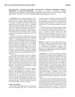
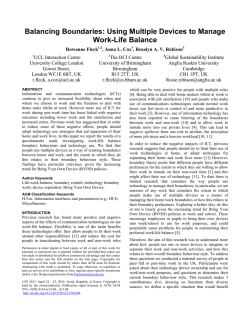
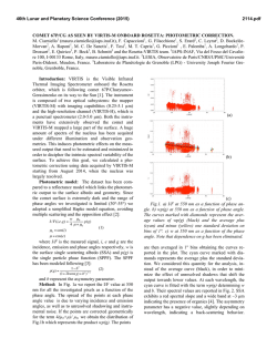
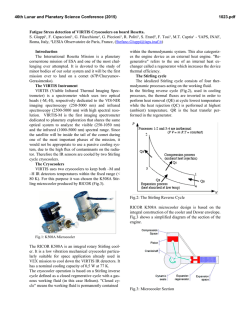
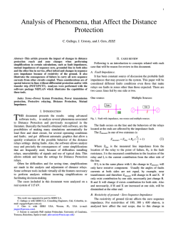
SLAC-PUB-15231
Surface Impedance Formalism for a Metallic
Beam Pipe with Small Corrugations
G. Stupakov, K. L. F. Bane
SLAC
Abstract
A metallic pipe with wall corrugations is of special interest in light of recent proposals to use
such a pipe for the generation of terahertz radiation and for energy dechirping of electron bunches
in free electron lasers. In this paper we calculate the surface impedance of a corrugated metal wall
and show that it can be reduced to that of a thin layer with dielectric constant and magnetic
permeability µ. We develop a technique for the calculation of these constants, given the geometrical
parameters of the corrugations. We then calculate, for the specific case of a round metallic pipe
with small corrugations, the frequency and strength of the resonant mode excited by a relativistic
beam. Our analytical results are compared with numerical simulations, and are shown to agree
well.
Work supported by US Department of Energy contract DE-AC02-76SF00515.
SLAC National Accelerator Laboratory, Menlo Park, CA 94025
I.
INTRODUCTION
Calculation of the impedance due to beam interaction with the walls of a vacuum chamber
is an important part of the design of modern accelerators. In some cases the elements of the
vacuum chamber that generate the beam impedance are small and uniformly distributed over
the surface of the wall. One example of such an impedance is that due to surface roughness,
which may be important, for example, in undulator vacuum chambers of modern x-ray
free electron lasers [1–4]. Another example is a vacuum chamber surface with many small,
approximately uniformly distributed holes [5, 6]. While exact calculation of the impedance
in such cases can be extremely difficult or may even be impossible due to the smallness of
the individual perturbations and their large number, the combined effect on the beam can
often be represented by a so-called surface impedance. The situation here is analogous to
the effective boundary condition introduced in electrodynamics when the skin depth in the
metal (at a given frequency) is much smaller than the thickness of the metal wall and the
wavelength of the electromagnetic field—the so-called Leontovich boundary condition [7].
In the accelerator context the surface impedance was previous employed by Balbekov for
the treatment of small obstacles in a vacuum chamber [8, 9]. For a rough surface it was
introduced by M. Dohlus [10] and also studied in [6].
The subject of this paper is how to use a surface impedance formalism to represent the
beam-cavity interaction of a metal wall with small corrugations. A metallic pipe with wall
corrugations is of special interest in light of recent proposals to use pipes with corrugated
surfaces for the generation of terahertz radiation [11], and for energy dechirping of electron
bunches in free electron lasers [12]. Following these papers, we will focus on the case of
r
b
z
FIG. 1. A round pipe of radius b with rectangular corrugations in the wall.
2
azimuthally symmetric, rectangular corrugations in a round pipe as shown in Fig 1. Note,
however, that the surface impedance method of representing boundary corrugations is applicable more generally to geometries that are not round.
This paper is organized as follows: In Section II we show how a corrugated wall can
be replaced by an equivalent thin layer which has a dielectric constant and a magnetic
permeability µ, and connect the values of and µ to the properties of the corrugations. While
µ can easily be calculated for given parameters of the corrugations, finding requires the
solution of a two-dimensional electrostatic problem. The solution to this problem is obtained
in Section III. In Section IV we reformulate the boundary condition on the wall in the more
general terms of a surface impedance. Using the derived boundary condition, in Section V,
we calculate, for the case of a corrugated waveguide in round geometry, the frequency and
strength of the resonant mode that is excited by a relativistic beam. In Section VI we
compare the theoretical results with simulations, and in Section VII we discuss our main
results. The derivation in the main text of the surface boundary conditions is somewhat
intuitive in nature; in Appendix A we give a more formal derivation. Finally, in Appendix B
we derive properties of the resonant mode in a round metallic pipe with a thin dielectricmagnetic liner.
Throughout this paper we work in Gaussian units.
II.
METAL SURFACE WITH PERIODIC RECTANGULAR CORRUGATIONS
We consider a metal surface with periodic corrugations of period p, depth h and width
g. As was shown in [13], an electromagnetic field interacting with a small indentation in a
metal wall induces electric and magnetic dipoles that are proportional to the strength of the
electric field at the location of the indentation. Treating a corrugated wall as a sequence
of indentations, we expect that it can be characterized by magnetic and electric moments
per unit area. When the size of the corrugations is much smaller than the reduced wavelength of the electromagnetic field, λ = λ/2π, its electrodynamic properties can effectively
be described by the averaged values of these moments. Since a thin layer which possesses
dielectric and magnetic properties acquires electric and magnetic moments in an external
electromagnetic field, we can equivalently replace the corrugations with such a layer, characterizing it by a dielectric constant and a magnetic permeability µ (see Fig. 2). In this
3
Section we will show how to connect the values of and µ to the geometrical shape of the
corrugations.
For our geometry, we expect the dielectric-magnetic model to be applicable when the
corrugation period is much smaller than the reduced wavelength of the electromagnetic
field,
p λ.
(1)
In what follows, we will also assume that all dimensions of the corrugations are much smaller
than the pipe radius b,
p, h b,
(2)
which will allow us to treat the corrugated surface as locally flat. The coordinate y is
y
B
p-g
C
y
F
D
Ε ,Μ
h
x
g
A
G
FIG. 2. Corrugated surface and the equivalent dielectric-magnetic layer that replaces it in the
effective boundary condition.
perpendicular to the surface, directed to vacuum and is measured from the bottom of the
corrugations, as shown in Fig. 2.
We assume that the magnetic induction B0 is perpendicular to the plane x, y in Fig. 2 and,
being tangential to the metal surface, freely penetrates between the corrugation teeth. The
effective magnetic permeability µ of the equivalent layer is easy to find using the following
argument. Consider the region 0 < y < h of the corrugations and calculate the volume
averaged magnetic induction hBi in it. Because the magnetic field is expelled from the
metal of the teeth,
g
hBi = B0 .
p
(3)
For a magnetic layer with the magnetic permeability µ the relation between the tangential
component of the magnetic induction in the layer Bl and the magnetic field Hl is Bl = µHl .
4
Due to continuity of vector H on the boundary between the layer and vacuum, it is equal to
the magnetic induction B0 outside of the layer, Hl = B0 , and hence Bl = µB0 . The quantity
Bl inside the layer is to be associated with the averaged value of the magnetic field hBi
inside the corrugated area, Bl → hBi. Using (3) we then find that the effective permeability
of the corrugated surface is equal to the fraction of the area not occupied by the metal
g
µ= .
p
(4)
We see that µ does not depend on depth h; note also that µ < 1.
To calculate the effective dielectric constant we need to find the electric field in the
vicinity of (and inside) the corrugations. Due to the condition (1), in a small region near
the wall, |x|, y λ, one can neglect the time dependence and consider the electric field as
static, governed by an electrostatic potential φ(x, y), with E = −∇φ, which satisfies the
Laplace equation. Compared to a flat metal surface where the boundary condition requires
the electric field to be directed perpendicular to the surface, in case of corrugations, the
electric field deviates from the normal direction at y ∼ h. At a large distance from the
corrugated surface, however, where y h (but still y b), E is almost parallel to the
ˆ . Mathematically it means that the electrostatic potential φ satisfies the
y axis, E → E0 y
boundary condition at infinity:
φ → −E0 y + φ0 , when y → ∞.
(5)
The other boundary condition for φ is φ = 0 on the surface of the metal.
The value of the constant φ0 in (5) is directly related to of the equivalent dielectric
layer. Indeed, the electric field inside the dielectric layer is equal to E0 /, with E0 the normal
electric field outside of the layer. Given φ = 0 at y = 0 we find that the potential drop in
the layer is −hE0 / and hence the potential outside of the layer is φ = −hE0 / − E0 (y − h).
Equating this expression to (5) we find
1−
1
φ0
=
.
hE0
(6)
In the next Section we will show how to calculate φ0 using the conformal mapping technique,
and thus express in terms of the geometric parameters g, h and p.
Our main results equations (4) and (6) can be also derived in a more formal way from
Maxwell’s equations. Such a derivation is given in Appendix A.
5
III.
SOLVING THE LAPLACE EQUATION AND CALCULATING THE DIELEC-
TRIC CONSTANT
We need to solve the Laplace equation
∂ 2φ ∂ 2φ
+
= 0,
∂x2 ∂x2
(7)
with the boundary condition φ = 0 on the surface of the metal and the asymptotic relation (5) at infinity. The function φ is periodic along x with the period p, and symmetric
with respect to the vertical symmetry lines of the corrugation pattern (two such lines, AB
and CD, are shown in Fig. 2). Given the symmetry of the boundary, it is sufficient to find
the solution of (7) in the domain shown in Fig. 3. The boundary conditions for φ in this
B
C
F
D
y
A
G
x
FIG. 3. The domain of solution of equation (7) is bounded by the red line (the letters along the
line establish the correspondence with the area ABCDFG depicted in Fig. 2). Also shown is the
local coordinate system x, y with the origin located at point A.
domain are φ = 0 on lines AG, GF and FD (metal surfaces) and ∂φ/∂x = 0 on AB and CD
(symmetry lines).
One can find the solution of (7) in the domain shown in Fig. 3 with the help of the conformal mapping technique using the Schwartz-Christoffel integral [14]. For this we introduce
the dimensionless complex variables w = ψ¯ + iφ¯ and z = y¯ + i¯
x, where
x¯ =
2x
,
p
y¯ =
2y
,
p
2φ
φ¯ = −
,
pE0
(8)
with x and y the local coordinates shown in Fig. 3, and ψ¯ an auxiliary function which we
¯ the asymptotic
will not use in what follows. Note that with these definitions of y¯ and φ,
6
dependence (5) is cast into φ¯ = y¯ + φ¯0 with φ¯0 = −2φ0 /pE0 . The required conformal
map, z = f (w), is defined by a complex analytical function f whose inverse, f −1 , gives the
¯ x, y¯) = Imf −1 (¯
normalized potential, φ(¯
y + i¯
x). Omitting the derivation, we present here the
expression for f (w) [15]:
s
u−A
B(A − 1)
A−1
B(A − 1)
2
(B − A)F µ,
+ (1 − B)Π
, µ,
,
f=
π (A − B)(A − u)
(A − B)
A−B
(A − B)
(9)
where u = 14 e−πw (1 + eπw )2 , and
s
µ = arcsin
(A − B)(1 − u)
(A − 1)(B − u)
!
.
(10)
Here F (µ, τ ) is the elliptic integral of the first kind, Π(ξ, µ, τ ) is the incomplete elliptic
integral of the third kind [16], and A and B (A < B) are numbers related to the geometric
parameters p, g and h. These numbers are found from the following two equations:
g
Im lim f (w) = ,
w→A
p
Re lim f (w) = −
w→A
2h
.
p
(11)
While the equation for f seems complicated, it can easily be solved with modern computational software programs such as Mathematica [17].
As a practical example we consider parameters of the corrugations considered in Ref. [12]:
h = 0.45 mm, p = 1 mm, g = 0.75 mm. Solving equations (11) one finds A = 0.430,
B = 0.965. Equipotential lines derived from Eq. (9) are shown in Fig. 4 and the dependence
¯ y ) at x¯ = 0 is shown in Fig. 5. One can see that as y¯ → ∞, the dependence φ(¯
¯ y ) indeed
φ(¯
approaches a linear profile φ¯ = y¯ + φ¯0 , in agreement with (5). The numerical value of the
¯ we find that
constant φ¯0 = −0.7. Recalling the definition (8) of the normalized variable φ,
φ0 /E0 p = 0.35 which gives for the value of in (6), = 4.5. The value of µ for this case is
µ = g/p = 0.75.
IV.
SURFACE IMPEDANCE
Having replaced the corrugations by a thin layer with dielectric and magnetic properties
we can now derive an effective boundary condition on the surface of the metal due to the
layer. For this we assume that the electric field in the system lies in the x, y plane and
7
1.4
1.2
2y/p
1.0
0.8
0.6
0.4
0.2
0.0
0.0 0.2 0.4 0.6 0.8 1.0
2x/p
FIG. 4. Equipotential lines (blue) in a half-cell of the corrugations.
3.0
2.5
_
Φ
2.0
1.5
1.0
0.5
0.0
0
1
2
3
_
y
FIG. 5. Dimensionless potential φ¯ versus y¯ for x = 0 (solid line). The broken line is φ¯ = y¯. The
vertical distance between the two lines for large values of y¯ is equal to φ¯0 .
the magnetic field is directed along z. We will also assume that all the fields depend on
time and coordinate x through the factor e−iωt+ikx . These assumptions are adequate for
calculation of the longitudinal impedance of a beam propagating along the axis of the pipe
with a corrugated wall.
8
It follows from Maxwell’s equations that inside the layer Ex satisfies the following equation
ω k 2 c2 −1
∂Ex
=i
− µ Hz .
(12)
∂y
c
ω2
Because the layer is thin, we can integrate this equation using the boundary condition on
the surface of the metal, Ex |y=0 = 0, and assuming that the magnetic field is approximately
constant within the layer,
Ex |y=h
ω
≈ ih
c
k 2 c2 −1
− µ Hz .
ω2
(13)
This relation can be considered as an effective boundary condition at y = h.
If we now consider the axisymmetric geometry of the pipe shown in Fig. 1, and use the
cylindrical coordinate system r, θ, z, then the boundary condition (13) is set at r = b−h ≡ a.
Replacing the local components of the fields in (14) by the corresponding components in the
cylindrical system, Ex → Ez and Hz → −Hθ , we arrive at the following boundary condition
Ez |r=a = −ζHθ |r=a ,
where we have introduced the surface impedance ζ,
ω k 2 c2 −1
−µ .
ζ(ω, k) = ih
c
ω2
(14)
(15)
In the particular case of waves propagating with the speed of light along the axis of the pipe
ω = kc, Eq. (15) simplifies to
ζ = ih
ω −1
−µ .
c
(16)
In this form the expression for ζ was introduced in [6].
Note the similarity of (14) with the so-called Leontovich boundary condition on the
surface of a good conductor [7] which for our case will have the same form as (14), but with
p
ζ = (1 − i) ω/8πσ, where σ is the conductivity of the metal.
V.
BEAM IMPEDANCE AND SYNCHRONOUS MODE
Given the boundary condition (14) one can solve Maxwell’s equations for a relativistic
beam propagating along the axis of the pipe and find the longitudinal impedance. This
problem has been addressed in several papers in the past [6, 18–20]. Here we summarize the
9
main results of such analysis. For completeness, a detailed derivation of the resonant mode
is given in Appendix B.
A round pipe with a thin magnetic-dielectric layer supports the propagation of an axisymmetric mode with the phase velocity equal to the speed of light, i.e., ω = kc. The
frequency of this mode ω0 is given by
s
ω0 = c
2
.
ah(µ − −1 )
(17)
Such a mode resonantly interacts with a relativistic beam and generates a wake field (for a
point charge) equal to
w(s) = 2κloss cos(ω0 s/c),
(18)
where κloss is the loss factor associated with the mode. In the lowest approximation the loss
factor is given by (see derivation in Appendix B)
κloss =
2
.
a2
(19)
The group velocity of the mode vg (an important parameter when considering the pipe as a
terahertz source [11]) is close to the speed of light, and given by (see Appendix B)
1 − βg = 4
h
µ − −1 ,
a
(20)
where βg ≡ vg /c. For completeness we should also mention that, because of the finite
resistivity of the walls, resistive wall heating will accompany the mode. The analytical
calculation of this effect can be found in Ref. [11] and will not be discussed further here.
Note that an expression for the mode frequency obtained in Ref. [20] neglects the term
−1 in (17) and is obtained from that equation in the limit −1 → 0, if one uses (4) for µ.
As an illustration, we can now evaluate the frequency and the loss factor of the synchronous mode for a corrugated structure of Ref. [12]. The parameters are: h = 0.45 mm,
p = 1 mm, g = 0.75 mm, b = 3.45 mm (and hence a = 3 mm). Taking = 4.5 and µ = 0.75
as calculated in the previous section and using (17) we find for the wavelength of the mode
λ = 2πc/ω0 = 3.8 mm. Simulations reported in [12] give λ = 4.4 mm, in satisfactory
agreement with our theory. Note that for this case the period p is actually larger than the
reduced wavelength λ/2π, so a noticeable deviation of the analytical λ from the simulated
one is not surprising. For the loss factor Eq. (19) predicts κloss = 1 MV/(nC·m) while the
simulations give κloss = 1.36 MV/(nC·m).
10
VI.
COMPARISON WITH SIMULATIONS
To compare our analytical results with the direct solution of Maxwell’s equation we
calculated the wavelength and the loss factors for several cases of small corrugations. All
have the same values p = 1 mm, g = 0.75 mm and b = 3.45 mm, with h varying from
75 to 225 µm. Numerical results were obtained by running the computer code KN7C, a
program that uses field matching to find the longitudinal modes in a periodic, disk-loaded
structure [21].
Figure 6 compares the frequency of the resonant mode for five different values of h. There
is good agreement between theory and simulation at larger values of h, with a discrepancy
at the level of 10% for the smallest h. This is expected because the ratio λ/p decreases with
decreasing h from 0.92 at h = 225 µm to 0.43 at h = 75 µm, and hence (1) is violated more
at smaller h.
æ
240
220
æ
f (GHz)
200
180
æ
æ
160
æ
æ
140
120
æ
æ
æ
æ
80
100
120
140
160
180
200
220
h (Μm)
FIG. 6. Frequency of the resonant modes for five different values of h indicated by dots. Red color
shows the theoretical values, blue color is simulations with KN7C.
Figure 7 compares the theoretical and numerical loss factors. We see that the loss factor
is more sensitive to the marginal fulfillment of condition (1); the theoretical result exceeds
the simulated one by 30-40%.
11
2.0
Κ (MV/nC/m)
1.5
æ
æ
æ
æ
æ
æ
æ
æ
æ
æ
1.0
0.5
0.0
80
100
120
140
160
180
200
220
h (Μm)
FIG. 7. The dependence of the loss factors versus h. Red color shows the theoretical values
computed with Eq. (19), blue color is simulations with KN7C.
VII.
DISCUSSION
Our theoretical approach developed in Sections II and III can be generalized to other
shapes of corrugations. While the magnetic permeability is easily calculated as a relative
area of vacuum region in the corrugations, the electrostatic part of the problem involves
the solution of Laplace’s equation for the given shape. For some shapes (for examples
triangular corrugations) the solution can again be found with the help of the conformal
mapping technique, while for more complicated shapes it can be found numerically. In any
case, the derived values of µ and can then be substituted into the boundary condition (14)
and (15) and used in the calculation of wakefields.
One advantage of our theory is that it allows for direct comparison with metallic tubes
lined with a thin dielectric layer, another approach for generating terahertz radiation [22].
Indeed, the main characteristic of the radiation—its frequency—is expressed by Eq. (17)
through the effective values of and µ. For a pipe with wall corrugations these parameters
are calculated as described in this paper, for the dielectric structure is just the electric
permeability for the dielectric (e.g., = 3.8 for the fused silica used in [22]), and µ is typically
close to 1.
While our emphasis in this paper has been on pipes with round geometry, one can also
12
use the effective boundary condition (13) for pipes of different cross sections. As was pointed
out in [12], for an adjustable dechirper, one can consider using parallel metallic plates
with corrugations, which makes the cross section of the pipe rectangular. Electromagnetic
propertied of such a structure were analyzed in Ref. [23] through a mode matching technique;
the method developed in this paper offers an alternative, easier approach to the problem.
VIII.
ACKNOWLEDGEMENTS
This work was supported by US DOE contracts DE-AC03-76SF00515.
[1] K. L. F. Bane, C. K. Ng, and A. W. Chao, Estimate of the impedance due to wall surface
roughness, Report SLAC-PUB-7514 (SLAC, 1997).
[2] A. Novokhatski and A. Mosnier, in Proceedings of the 1997 Particle Accelerator Conference
(IEEE, Piscataway, NJ, 1997) pp. 1661–1663.
[3] G. V. Stupakov, Phys. Rev. ST Accel. Beams 1, 064401 (1998).
[4] K. L. F. Bane and A. Novokhatskii, The Resonator impedance model of surface roughness
applied to the LCLS parameters, Tech. Rep. SLAC-AP-117 (SLAC, 1999).
[5] S. Petracca, Tech. Rep. CERN-SL-99-003, (CERN, 1999).
[6] G. V. Stupakov, in Workshop on Instabilities of High Intensity Hadron Beams in Rings, AIP
Conference Proceedings No. 496, edited by T. Roser and S. Y. Zhang (American Institute of
Physics, Upton, New York, 1999) pp. 341–350.
[7] L. D. Landau and E. M. Lifshitz, Electrodynamics of Continuous Media, 2nd ed., Course of
Theoretical Physics, Vol. 8 (Pergamon, London, 1960) (Translated from the Russian).
[8] V. I. Balbekov, On using equivalent circuits for calculation of longitudinal beam coupling
impedance of a ring accelerator. I. A single insertion, (in Russian), Tech. Rep. IFVE-93-55
(Inst. for High Energy Physics, Protvino, Russia, 1993).
[9] V. I. Balbekov, On using equivalent circuits for calculation of longitudinal beam coupling
impedance of a ring accelerator. II. Symmetric system, (in Russian), Tech. Rep. IFVE-93-56
(Inst. for High Energy Physics, Protvino, Russia, 1993).
[10] M. Dohlus, (1999), private communications.
13
[11] K. L. F. Bane and G. Stupakov, Nuclear Instruments and Methods in Physics Research Section
A: Accelerators, Spectrometers, Detectors and Associated Equipment 677, 67 (2012).
[12] K. Bane and G. Stupakov, Nuclear Instruments and Methods in Physics Research Section A:
Accelerators, Spectrometers, Detectors and Associated Equipment 690, 106 (2012).
[13] S. S. Kurennoy and G. V. Stupakov, Particle Accelerators 45, 95 (1994).
[14] C. Ruel V and J. W. Brown, Complex variables and applications, 5th ed. (McGraw-Hill, 1989).
[15] K. Bane and G. Stupakov, in Proceedings of the 28th International Free Electron Laser Conference (FEL 2006) (Edinburgh, UK, 2006) p. THPCH076.
[16] F. W. J. Olver, D. W. Lozier, R. F. Boisvert, and C. W. Clark, eds., ”NIST Handbook of
Mathematical Functions” (Cambridge University Press, 2010).
[17] Wolfram Research, Inc., Mathematica, version 8.0 ed. (Wolfram Research, Inc., 2011).
[18] A. V. Burov and A. V. Novokhatskii, The Device for Bunch Self-Focussing, Tech. Rep.
BUDKERINP-90-28 (Budker Inst. of Nucl. Physics, Novosibirk, Russia, 1990).
[19] K.-Y. Ng, Part. Accel. 25, 153 (1990).
[20] K. Bane and G. Stupakov, in 20th International Linac Conference (Linac 2000), Vol. 1 (Monterey, California, 2000) pp. 92–94.
[21] E. Keil, Nucl. Instr. Meth. 100, 419 (1972).
[22] A. M. Cook et al., Phys. Rev. Lett. 103, 095003 (2009).
[23] K. L. F. Bane and G. V. Stupakov, Phys. Rev. ST Accel. Beams 6, 024401 (2003).
Appendix A: Formal derivation of boundary conditions
We consider the plane geometry shown in Fig. 2 and assume the time dependence e−iωt
for Ex , Ey and Hz , which are functions of x and y. Our goal is to solve Maxwell’s equations
in the vicinity of the corrugations and obtain asymptotic expressions for the fields in the
limit y h. Given condition (1) we consider the wave number k and the ratio ω/c (assumed
of the same order), as small parameters in the theory, and put a formal smallness factor ς
in front of them. This allows us to easily track the relative orders of magnitude of various
terms in equations. In the final result we will set ς = 1.
The two Maxwell equations for the electric field in vacuum which we need for the deriva14
tion are
ω
(∇ × E)z = iς Hz ,
c
∇ · E = 0.
(A1)
The equation for the magnetic field ∇ × H = −iςωE/c shows that the change in Hz is
of the first order and since Hz enters into (A1) multiplied by the smallness parameter ς,
account of its variation results in the second order terms which we neglect. Hence Hz can
be considered as locally constant in the equations.
At large distance from the corrugations, formally when y → ∞, the fields should match
those in a wave traveling along x with wavenumber k. This requirement suggests the following form for the fields
Hz = H0 eiςkx ,
ˆ × ∇χ)eiςkx ,
E = (−∇φ + ς z
(A2)
where φ(x, y) and χ(x, y) are periodic functions in x with the period p. Note that we assign
the smallness parameter ς to the solenoidal part of the field in (A2) in comparison with
the potential term −∇φ. We will see that equations support this scaling. Since we neglect
variations of the magnetic field, H0 is a constant in our approximation.
Substituting (A2) into ∇ · E = 0 we obtain
∇ · E = −eiςkx ∆φ − iςk
∂φ iςkx
e
+ O(ς 2 ) = 0.
∂x
(A3)
In the lowest order approximation (A3) reduces to
∆φ = 0,
(A4)
with the boundary conditions φ = 0 at the surface of the metal and (5) at y → ∞.
Substituting (A2) into the first equation in (A1) and neglecting second order terms we
obtain
ω
∂φ
∆χ = i Hz + ik .
c
∂y
(A5)
The boundary condition for χ is the vanishing normal derivative, ∂χ/∂n = 0, at the surface
of the metal. At large distance from the corrugations, y → ∞, the derivative −∂χ/∂y tends
to a constant value equal to the electric field Ex induced by the corrugation. It turns out
however that one does not need to solve (A5) in order to find the x component of the electric
field Ex far from the corrugations. For this one needs to integrate (A5) over the vacuum
15
area Σ limited by the metal surface on one side and by a straight line y = y0 with y0 h
on the other. We will assume that this area extends along x from x = 0 to x = l where l is
equal to an integer number of periods, l = N p. We have
Z
Z
ω
dx dy + iklφy=y0 ,
∆χdx dy = i Hz
c
Σ
Σ
(A6)
where in the last term on the right hand side we used the boundary condition on the metal
φ = 0 and took into account that at y = y0 according to (5) φ does not depend on x.
Using Green’s identity, periodicity of χ along x, and the boundary condition ∂χ/∂n = 0
on the metal, it is easy to show that the integral on the left hand side of (A6) is equal to
l∂χ/∂y|y=y0 = −(l/ς)Ex |y=y0 (Ex at large y does not depend on x). Also noting that the
R
area Σ dx dy = l[y0 − h(1 − g/p)] and φy=y0 = −y0 E0 + φ0 we obtain
ω
g
−Ex |y=y0 = iς H0 y0 − h 1 −
+ iςk(−y0 E0 + φ0 ).
(A7)
c
p
Note that E0 and H0 , being fields in a plane electromagnetic wave, are related through
E0 = kcH0 /ω casting (A7) into
−Ex |y=y0
ω
k 2 c2
g
= iς H0 y0 1 − 2 − h 1 −
+ iςkφ0 .
c
ω
p
(A8)
Eq. (A8) should be understood as a matching condition between the region near the
corrugations and the field far from the wall. The value of y0 can be chosen arbitrarily in
the region h y0 b. We can also treat (A8) as a formal boundary condition setting, for
example, y0 = h. While this choice of y0 is inconsistent with the exact field distribution at
y0 = h, considered as a boundary condition, it will correctly define the fields far from the
corrugations. Setting y0 = h in (A8) and ς = 1 we obtain
ω
g k 2 c2
−Ex |y=h = ih H0
− 2 + ikφ0 .
c
p
ω
With a formal definition of and µ according to (4) and (6), Eq. (A9) reduces to
ω
k 2 c2 −1
−Ex |y=h = ih H0 µ − 2 ,
c
ω
(A9)
(A10)
in agreement with (14).
Appendix B: Resonant modes in a pipe coated with dielectric-magnetic layer
In this Appendix we study resonant modes propagating with the phase velocity equal
to the speed of light in a round pipe coated with a thin layer which is characterized by a
16
dielectric constant and a magnetic permeability µ. We will assume a vacuum region at
0 < r < a and the layer at a < r < b with the layer thickness h = b − a a. The metal
wall is located at r = b.
We start from Maxwell’s equations in vacuum,
∇×H =
1 ∂E
,
c ∂t
∇×E =−
1 ∂H
.
c ∂t
(B1)
Assuming Eθ , Hr , Hz = 0, and all non-zero components of the fields ∝ e−iωt+ikz , we arrive
at the wave equation for Ez
1 ∂ ∂Ez
r
+
r ∂r ∂r
ω2
2
− k Ez = 0.
c2
(B2)
The solution of (B2) in the region 0 < r < a is
Ez = AJ0 (κr),
with κ =
p
(B3)
ω 2 /c2 − k 2 . For Hθ in vacuum we find
c
Hθ = −i
ω
−1
∂Ez
k 2 c2
ω
−1
= −i AJ1 (κr).
2
ω
∂r
κc
(B4)
Using (B3) and (B4) and the boundary condition (14) we arrive at the dispersion relation
for the mode
h
J0 (κa) =
κ
ω2
2 −1
µ−k J1 (κa).
c2
(B5)
Note that for a resonant mode ω = kc and κ = 0. In this case one has to take the limit
limκ→0 κ−1 J1 (κa) = a/2 on the right hand side of (B5) which gives the dispersion relation
iωa
ζ(ω, ω/c) = 1.
2c
(B6)
The solution to this equation ω = ω0 is given by (17). The electromagnetic field in the
resonant mode can be shown to be (see, e.g., [6])
r
Er = Hθ = E0 e−iω0 t+ikz ,
a
Ez = E0
2i −iω0 t+ikz
e
,
ka
(B7)
with E0 the wave amplitude.
To find the loss factor κloss for the mode we will use the formula from [23],
κloss =
2
Ez0
(1 − βg )−1 ,
4u
17
(B8)
where u is the electromagnetic energy per unit length in the mode, Ez0 is the amplitude of
the longitudinal electric field on axis, and βg = vg /c, with vg = dω/dk the group velocity.
The group velocity is computed by differentiating the dispersion relation (B5) which can be
written as
J0 (κa) =
iω
ζ(ω, k)J1 (κa).
cκ
(B9)
The calculations are simplified if we note that we need the dispersion relation close to the
point κ = 0 and expand (B9) assuming that κa 1:
1
J0 (κa) ≈ 1 − κ2 a2 ,
4
J1 (κa)
1
1
≈ − κ2 a2 ,
κa
2 16
(B10)
1 2 2
1 iωa
1 iωa
ζ(ω, k) = κ a 1 −
ζ(ω, k) .
1−
2 c
4
4 c
(B11)
and rewriting (B9) as
Because the right hand side of this equation is of the second order in κa we can replace
ζ(ω, k) there by ζ(ω, ω/c) which can then be eliminated with the help of (B6):
1 iωa
1 2 ω2
2
1−
ζ(ω, k) = a
−k .
2 c
8
c2
(B12)
Differentiating (B12) with respect to k and setting in the result ω = ck we obtain
1
−h vg µ − c−1 = a (vg − c) .
4
(B13)
Because we assume h small, vg on the left hand side can be replaced by c and the equation
solved for vg ,
1 − βg = 4
h
µ − −1 .
a
(B14)
From this solution we see that indeed vg is close to the speed of light.
To calculate the energy in the mode u we use Eqs. (B7) in which we drop the exponential
factor e−iω0 t+ikz , and set a unit field amplitude, E0 = 1,
r
Er0 = Hφ0 = ,
a
Ez0 =
2ic
.
ω0 a
(B15)
To the lowest approximation the energy in the mode is computed by integrating the energy
density in the vacuum region
1
u=
16π
Z
a
2
2πrdr(Er0
0
18
+
2
Hφ0
)
a2
= ,
16
(B16)
(an additional factor
1
2
in this equation comes from the averaging over time). Note that we
neglected the Ez field in (B16) because it is much smaller than Er and Eφ . Substituting (B14)
and (B16) into (B8) we obtain
κloss =
where we also used (17).
19
2
,
a2
(B17)