
Riemannian Manifolds: An Introduction to Curvature
Graduate Texts in Mathematics
TAKE~~~~AIUNG.
Introduction to
Axiomatic Set Theory. 2nd ed.
OXTOBY.Measure and Category. 2nd ed.
SCHAEFER.Topological Vector Spaces.
HILTONISTAMMBACH.
A Course in
Homological Algebra. 2nd ed.
MACLANE.Categories for the Working
Mathematician.
HUGWPPER.Projective Planes.
SERRE.A C o m e in Arithmetic.
TAKE~~~~AIUNG.
Axiomatic Set Theory.
HUMPHREYS.Introduction to Lie Algebras
and Representation Theory.
COHEN.A Course in Simple Homotopy
Theory.
CONWAY.
Functions of One Complex
Variable I. 2nd ed.
B'EALS. Advanced Mathematical Analysis.
ANDERSON/FWLLER.
Rings and Categories
of Modules. 2nd ed.
G O L U B ~ ~ S K YStable
/ G ~Mappings
.
and Their Singularities.
BERBERIAN.
Lectures in Functional
Analysis and Operator Theory.
W m . The Structure of Fields.
ROSENBLATT.
Random Processes. 2nd ed.
HALMos. Measure Theory.
HALMos. A Hilbert Space Problem Book.
2nd ed.
HUSEMOLLER.
Fibre Bundles. 3rd ed.
HUMPHREYS.
Linear Algebraic Groups.
B A R N ~ M A CAn
K . Algebraic Introduction
to Mathematical Logic.
GREUB.Linear Algebra. 4th ed.
HOLIUIES.
Geometric Functional Analysis
and Its Applications.
HEW~~~/STROMBERG.
Real and Abstract
Analysis.
MANES.Algebraic Theories.
KFLLEY. General Topology.
ZARISKI~SAMIJEL. Commutative Algebra.
V0l.I.
ZAR~SKJISAMLEL.Commutative Algebra.
v01.n.
JACOBSON.
Lectures in Abstract Algebra I.
Basic Concepts.
JACOBSON.
Lectures in Abstract Algebra
II. Linear Algebra.
JACOBSON.
Lectures in Abstract Algebra
III. Theory of Fields and Galois Theory.
HIRSCH.Differential Topology.
SP~IZER.
Principles of Random Walk.
2nd ed.
WERMER.Banach Algebras and Several
Complex Variables. 2nd ed.
KELLEY/NAMIoKAet d. Linear
Topological Spaces.
MONK.Mathematical Logic.
GRAUERT/FRI~ZSCHE.
Several Complex
Variables.
An Invitation to C-Algebras.
ARVESON.
KEMENYISNELLJKNAPP.
Denumerable
Markov Chains. 2nd ed.
APOSTOL.Modular Functions and
Dichlet Series in Number Theory.
2nd ed.
SERRE.Linear Representations of Finite
Groups.
G W J E R I S O N Rings
.
of Continuous
Functions.
KENDIG. Elementary Algebraic Geometry.
LoiVE. Probability Theory I. 4th ed.
LOEVE.Probability Theory II. 4th ed.
MOISE.Geometric Topology in
Dimensions 2 and 3.
S ~ m s M r u General
.
Relativity for
Mathematicians.
L i a r Geometry.
GRUENBER~~WEIR.
2nd ed.
EDWARDS.
Fennat's Last Theorem.
KLJNGENBERG.
A Course in Differential
Geometry.
HARTSHORNE.
Algebraic Geometry.
MANIN.A Course in Mathematical Logic.
G R A W A T K I N SCombinatorics
.
with
Emphasis on the Theory of Graphs.
BROWNJPEARCY.
Introduction to Operator
Theory I: Elements of Functional
Analysis.
MASSEY.Algebraic Topology: An
Introduction.
CROWELLJFOX.Introduction to Knot
Theory.
K O B L ~p-adic
.
Numbers, padic
Analysis, and Zeta-Functions. 2nd ed.
LANG.Cyclotomic Fields.
ARNOLD.Mathematical Methods in
Classical Mechanics. 2nd ed.
continued afer index
John M. Lee
Riemannian Manifolds
An Introduction to Curvature
With 88 Illustrations
Springer
John M. Lee
Department of Mathematics
University of Washington
Seattle, W A 981 95-4350
USA
Editorial Board
S. Axler
Department of
Mathematics
Michigan State University
East Lansing, M I 48824
USA
F.W. G e k n g
P.R. Halmos
Department of
Mathematics
University of Michigan
Ann Arbor, MI 48109
USA
Department of
Mathematics
Santa Clara University
Santa Clara, C A 95053
USA
Mathematics Subject Classification (1991): 53-01, 53C20
Library of Congress Cataloging-in-Publication Data
Lee, John M., 1950Reimannian manifolds : an introduction to curvature I John M. Lee.
cm. - (Graduate texts in mathematics ; 176)
p.
Includes index.
ISBN 0-387-98271-X (hardcover : alk. paper)
1. Reimannian manifolds. I. Title. 11. Series.
QA649.L397 1997
516.3'734~21
O 1997 Springer-Verlag New York, Inc.
All rights reserved. This work may not be translated or copied in whole or in part without the written
permission of the publisher (Springer-Verlag New York, Inc., 175 Fifth Avenue, New York, NY
10010, USA), except for brief excerpts in connection with reviews or scholarly analysis. Use in connection with any form of information storage and retrieval, electronic adaptation, computer software,
or by similar or dissimilar methodology now known or hereafter developed is forbidden.
The use of general descriptive names, trade names, trademarks, etc., in this publication, even if the
former are not especially identified, is not to be taken as a sign that such names, as understood by the
Trade Marks and Merchandise Marks Act, may accordingly be used freely by anyone.
ISBN 0-387-98271-X Springer-Verlag New York Berlin Heidelberg SPIN 10630043 (hardcover)
ISBN 0-387-98322-8 Springer-Verlag New York Berlin Heidelberg SPIN 10637299 (softcover)
To my family:
Pm, Nathan, and Jeremy Weizenbaum
Preface
This book is designed as a textbook for a one-quarter or one-semester graduate course on Riemannian geometry, for students who are familiar with
topological and differentiable manifolds. It focuses on developing an intimate acquaintance with the geometric meaning of curvature. In so doing, it
introduces and demonstrates the uses of all the main technical tools needed
for a careful study of Riemannian manifolds.
I have selected a set of topics that can reasonably be covered in ten to
fifteen weeks, instead of making any attempt to provide an encyclopedic
treatment of the subject. The book begins with a careful treatment of the
machinery of metrics, connections, and geodesics, without which one cannot
claim to be doing Riemannian geometry. It then introduces the Riemann
curvature tensor, and quickly moves on to submanifold theory in order to
give the curvature tensor a concrete quantitative interpretation. From then
on, all efforts are bent toward proving the four most fundamental theorems
relating curvature and topology: the Gauss–Bonnet theorem (expressing
the total curvature of a surface in terms of its topological type), the Cartan–
Hadamard theorem (restricting the topology of manifolds of nonpositive
curvature), Bonnet’s theorem (giving analogous restrictions on manifolds
of strictly positive curvature), and a special case of the Cartan–Ambrose–
Hicks theorem (characterizing manifolds of constant curvature).
Many other results and techniques might reasonably claim a place in an
introductory Riemannian geometry course, but could not be included due
to time constraints. In particular, I do not treat the Rauch comparison theorem, the Morse index theorem, Toponogov’s theorem, or their important
applications such as the sphere theorem, except to mention some of them
viii
Preface
in passing; and I do not touch on the Laplace–Beltrami operator or Hodge
theory, or indeed any of the multitude of deep and exciting applications
of partial differential equations to Riemannian geometry. These important
topics are for other, more advanced courses.
The libraries already contain a wealth of superb reference books on Riemannian geometry, which the interested reader can consult for a deeper
treatment of the topics introduced here, or can use to explore the more
esoteric aspects of the subject. Some of my favorites are the elegant introduction to comparison theory by Jeff Cheeger and David Ebin [CE75]
(which has sadly been out of print for a number of years); Manfredo do
Carmo’s much more leisurely treatment of the same material and more
[dC92]; Barrett O’Neill’s beautifully integrated introduction to pseudoRiemannian and Riemannian geometry [O’N83]; Isaac Chavel’s masterful
recent introductory text [Cha93], which starts with the foundations of the
subject and quickly takes the reader deep into research territory; Michael
Spivak’s classic tome [Spi79], which can be used as a textbook if plenty of
time is available, or can provide enjoyable bedtime reading; and, of course,
the “Encyclopaedia Britannica” of differential geometry books, Foundations of Differential Geometry by Kobayashi and Nomizu [KN63]. At the
other end of the spectrum, Frank Morgan’s delightful little book [Mor93]
touches on most of the important ideas in an intuitive and informal way
with lots of pictures—I enthusiastically recommend it as a prelude to this
book.
It is not my purpose to replace any of these. Instead, it is my hope
that this book will fill a niche in the literature by presenting a selective
introduction to the main ideas of the subject in an easily accessible way.
The selection is small enough to fit into a single course, but broad enough,
I hope, to provide any novice with a firm foundation from which to pursue
research or develop applications in Riemannian geometry and other fields
that use its tools.
This book is written under the assumption that the student already
knows the fundamentals of the theory of topological and differential manifolds, as treated, for example, in [Mas67, chapters 1–5] and [Boo86, chapters
1–6]. In particular, the student should be conversant with the fundamental
group, covering spaces, the classification of compact surfaces, topological
and smooth manifolds, immersions and submersions, vector fields and flows,
Lie brackets and Lie derivatives, the Frobenius theorem, tensors, differential forms, Stokes’s theorem, and elementary properties of Lie groups. On
the other hand, I do not assume any previous acquaintance with Riemannian metrics, or even with the classical theory of curves and surfaces in R3 .
(In this subject, anything proved before 1950 can be considered “classical.”) Although at one time it might have been reasonable to expect most
mathematics students to have studied surface theory as undergraduates,
few current North American undergraduate math majors see any differen-
Preface
ix
tial geometry. Thus the fundamentals of the geometry of surfaces, including
a proof of the Gauss–Bonnet theorem, are worked out from scratch here.
The book begins with a nonrigorous overview of the subject in Chapter
1, designed to introduce some of the intuitions underlying the notion of
curvature and to link them with elementary geometric ideas the student
has seen before. This is followed in Chapter 2 by a brief review of some
background material on tensors, manifolds, and vector bundles, included
because these are the basic tools used throughout the book and because
often they are not covered in quite enough detail in elementary courses
on manifolds. Chapter 3 begins the course proper, with definitions of Riemannian metrics and some of their attendant flora and fauna. The end of
the chapter describes the constant curvature “model spaces” of Riemannian
geometry, with a great deal of detailed computation. These models form a
sort of leitmotif throughout the text, and serve as illustrations and testbeds
for the abstract theory as it is developed. Other important classes of examples are developed in the problems at the ends of the chapters, particularly
invariant metrics on Lie groups and Riemannian submersions.
Chapter 4 introduces connections. In order to isolate the important properties of connections that are independent of the metric, as well as to lay the
groundwork for their further study in such arenas as the Chern–Weil theory
of characteristic classes and the Donaldson and Seiberg–Witten theories of
gauge fields, connections are defined first on arbitrary vector bundles. This
has the further advantage of making it easy to define the induced connections on tensor bundles. Chapter 5 investigates connections in the context
of Riemannian manifolds, developing the Riemannian connection, its geodesics, the exponential map, and normal coordinates. Chapter 6 continues
the study of geodesics, focusing on their distance-minimizing properties.
First, some elementary ideas from the calculus of variations are introduced
to prove that every distance-minimizing curve is a geodesic. Then the Gauss
lemma is used to prove the (partial) converse—that every geodesic is locally minimizing. Because the Gauss lemma also gives an easy proof that
minimizing curves are geodesics, the calculus-of-variations methods are not
strictly necessary at this point; they are included to facilitate their use later
in comparison theorems.
Chapter 7 unveils the first fully general definition of curvature. The curvature tensor is motivated initially by the question of whether all Riemannian metrics are locally equivalent, and by the failure of parallel translation
to be path-independent as an obstruction to local equivalence. This leads
naturally to a qualitative interpretation of curvature as the obstruction to
flatness (local equivalence to Euclidean space). Chapter 8 departs somewhat from the traditional order of presentation, by investigating submanifold theory immediately after introducing the curvature tensor, so as to
define sectional curvatures and give the curvature a more quantitative geometric interpretation.
x
Preface
The last three chapters are devoted to the most important elementary
global theorems relating geometry to topology. Chapter 9 gives a simple
moving-frames proof of the Gauss–Bonnet theorem, complete with a careful treatment of Hopf’s rotation angle theorem (the Umlaufsatz). Chapter
10 is largely of a technical nature, covering Jacobi fields, conjugate points,
the second variation formula, and the index form for later use in comparison theorems. Finally in Chapter 11 comes the d´enouement—proofs of
some of the “big” global theorems illustrating the ways in which curvature
and topology affect each other: the Cartan–Hadamard theorem, Bonnet’s
theorem (and its generalization, Myers’s theorem), and Cartan’s characterization of manifolds of constant curvature.
The book contains many questions for the reader, which deserve special
mention. They fall into two categories: “exercises,” which are integrated
into the text, and “problems,” grouped at the end of each chapter. Both are
essential to a full understanding of the material, but they are of somewhat
different character and serve different purposes.
The exercises include some background material that the student should
have seen already in an earlier course, some proofs that fill in the gaps from
the text, some simple but illuminating examples, and some intermediate
results that are used in the text or the problems. They are, in general,
elementary, but they are not optional—indeed, they are integral to the
continuity of the text. They are chosen and timed so as to give the reader
opportunities to pause and think over the material that has just been introduced, to practice working with the definitions, and to develop skills that
are used later in the book. I recommend strongly that students stop and
do each exercise as it occurs in the text before going any further.
The problems that conclude the chapters are generally more difficult
than the exercises, some of them considerably so, and should be considered
a central part of the book by any student who is serious about learning the
subject. They not only introduce new material not covered in the body of
the text, but they also provide the student with indispensable practice in
using the techniques explained in the text, both for doing computations and
for proving theorems. If more than a semester is available, the instructor
might want to present some of these problems in class.
Acknowledgments: I owe an unpayable debt to the authors of the many
Riemannian geometry books I have used and cherished over the years,
especially the ones mentioned above—I have done little more than rearrange their ideas into a form that seems handy for teaching. Beyond that,
I would like to thank my Ph.D. advisor, Richard Melrose, who many years
ago introduced me to differential geometry in his eccentric but thoroughly
enlightening way; Judith Arms, who, as a fellow teacher of Riemannian
geometry at the University of Washington, helped brainstorm about the
“ideal contents” of this course; all my graduate students at the University
Preface
xi
of Washington who have suffered with amazing grace through the flawed
early drafts of this book, especially Jed Mihalisin, who gave the manuscript
a meticulous reading from a user’s viewpoint and came up with numerous
valuable suggestions; and Ina Lindemann of Springer-Verlag, who encouraged me to turn my lecture notes into a book and gave me free rein in deciding on its shape and contents. And of course my wife, Pm Weizenbaum,
who contributed professional editing help as well as the loving support and
encouragement I need to keep at this day after day.
Contents
Preface
vii
1 What Is Curvature?
The Euclidean Plane . . . . . . . . . . . . . . . . . . . . . . . . .
Surfaces in Space . . . . . . . . . . . . . . . . . . . . . . . . . . .
Curvature in Higher Dimensions . . . . . . . . . . . . . . . . . .
2 Review of Tensors, Manifolds, and Vector Bundles
Tensors on a Vector Space . . . . . . . . . . . . . . . . . .
Manifolds . . . . . . . . . . . . . . . . . . . . . . . . . . .
Vector Bundles . . . . . . . . . . . . . . . . . . . . . . . .
Tensor Bundles and Tensor Fields . . . . . . . . . . . . .
1
2
4
8
.
.
.
.
11
11
14
16
19
.
.
.
.
.
23
23
27
30
33
43
4 Connections
The Problem of Differentiating Vector Fields . . . . . . . . . . .
Connections . . . . . . . . . . . . . . . . . . . . . . . . . . . . . .
Vector Fields Along Curves . . . . . . . . . . . . . . . . . . . . .
47
48
49
55
.
.
.
.
.
.
.
.
.
.
.
.
3 Definitions and Examples of Riemannian Metrics
Riemannian Metrics . . . . . . . . . . . . . . . . . . . . . . . .
Elementary Constructions Associated with Riemannian Metrics
Generalizations of Riemannian Metrics . . . . . . . . . . . . . .
The Model Spaces of Riemannian Geometry . . . . . . . . . . .
Problems . . . . . . . . . . . . . . . . . . . . . . . . . . . . . .
xiv
Contents
Geodesics . . . . . . . . . . . . . . . . . . . . . . . . . . . . . . .
Problems . . . . . . . . . . . . . . . . . . . . . . . . . . . . . . .
58
63
5 Riemannian Geodesics
The Riemannian Connection . . . . . . . . . . .
The Exponential Map . . . . . . . . . . . . . . .
Normal Neighborhoods and Normal Coordinates
Geodesics of the Model Spaces . . . . . . . . . .
Problems . . . . . . . . . . . . . . . . . . . . . .
.
.
.
.
.
.
.
.
.
.
.
.
.
.
.
.
.
.
.
.
.
.
.
.
.
.
.
.
.
.
.
.
.
.
.
.
.
.
.
.
.
.
.
.
.
6 Geodesics and Distance
Lengths and Distances on Riemannian Manifolds
Geodesics and Minimizing Curves . . . . . . . . .
Completeness . . . . . . . . . . . . . . . . . . . .
Problems . . . . . . . . . . . . . . . . . . . . . .
.
.
.
.
.
.
.
.
.
.
.
.
.
.
.
.
.
.
.
.
.
.
.
.
.
.
.
.
.
.
.
.
91
. 91
. 96
. 108
. 112
7 Curvature
Local Invariants . . . . . . . . . . . .
Flat Manifolds . . . . . . . . . . . .
Symmetries of the Curvature Tensor
Ricci and Scalar Curvatures . . . . .
Problems . . . . . . . . . . . . . . .
.
.
.
.
.
.
.
.
.
.
.
.
.
.
.
.
.
.
.
.
.
.
.
.
.
.
.
.
.
.
.
.
.
.
.
.
.
.
.
.
.
.
.
.
.
115
115
119
121
124
128
8 Riemannian Submanifolds
Riemannian Submanifolds and the Second Fundamental Form
Hypersurfaces in Euclidean Space . . . . . . . . . . . . . . . .
Geometric Interpretation of Curvature in Higher Dimensions
Problems . . . . . . . . . . . . . . . . . . . . . . . . . . . . .
.
.
.
.
.
.
.
.
131
132
139
145
150
9 The Gauss–Bonnet Theorem
Some Plane Geometry . . . . . .
The Gauss–Bonnet Formula . . .
The Gauss–Bonnet Theorem . .
Problems . . . . . . . . . . . . .
.
.
.
.
.
.
.
.
.
.
.
.
.
.
.
.
.
.
.
.
.
.
.
.
.
.
.
.
.
.
.
.
.
.
.
.
.
.
.
.
.
.
.
.
10 Jacobi Fields
The Jacobi Equation . . . . . . . . . . . . .
Computations of Jacobi Fields . . . . . . .
Conjugate Points . . . . . . . . . . . . . . .
The Second Variation Formula . . . . . . .
Geodesics Do Not Minimize Past Conjugate
Problems . . . . . . . . . . . . . . . . . . .
.
.
.
.
.
.
.
.
.
.
.
.
.
.
.
65
65
72
76
81
87
.
.
.
.
.
.
.
.
.
.
.
.
.
.
.
.
.
.
.
.
.
.
.
.
.
.
.
.
.
.
.
.
.
.
.
.
155
156
162
166
171
. . . .
. . . .
. . . .
. . . .
Points
. . . .
.
.
.
.
.
.
.
.
.
.
.
.
.
.
.
.
.
.
.
.
.
.
.
.
.
.
.
.
.
.
.
.
.
.
.
.
.
.
.
.
.
.
.
.
.
.
.
.
173
174
178
181
185
187
191
.
.
.
.
.
.
.
.
.
.
.
.
11 Curvature and Topology
193
Some Comparison Theorems . . . . . . . . . . . . . . . . . . . . 194
Manifolds of Negative Curvature . . . . . . . . . . . . . . . . . . 196
Contents
xv
Manifolds of Positive Curvature . . . . . . . . . . . . . . . . . . . 199
Manifolds of Constant Curvature . . . . . . . . . . . . . . . . . . 204
Problems . . . . . . . . . . . . . . . . . . . . . . . . . . . . . . . 208
References
209
Index
213
1
What Is Curvature?
If you’ve just completed an introductory course on differential geometry,
you might be wondering where the geometry went. In most people’s experience, geometry is concerned with properties such as distances, lengths,
angles, areas, volumes, and curvature. These concepts, however, are barely
mentioned in typical beginning graduate courses in differential geometry;
instead, such courses are concerned with smooth structures, flows, tensors,
and differential forms.
The purpose of this book is to introduce the theory of Riemannian
manifolds: these are smooth manifolds equipped with Riemannian metrics (smoothly varying choices of inner products on tangent spaces), which
allow one to measure geometric quantities such as distances and angles.
This is the branch of modern differential geometry in which “geometric”
ideas, in the familiar sense of the word, come to the fore. It is the direct
descendant of Euclid’s plane and solid geometry, by way of Gauss’s theory
of curved surfaces in space, and it is a dynamic subject of contemporary
research.
The central unifying theme in current Riemannian geometry research is
the notion of curvature and its relation to topology. This book is designed
to help you develop both the tools and the intuition you will need for an indepth exploration of curvature in the Riemannian setting. Unfortunately,
as you will soon discover, an adequate development of curvature in an
arbitrary number of dimensions requires a great deal of technical machinery,
making it easy to lose sight of the underlying geometric content. To put
the subject in perspective, therefore, let’s begin by asking some very basic
questions: What is curvature? What are the important theorems about it?
2
1. What Is Curvature?
In this chapter, we explore these and related questions in an informal way,
without proofs. In the next chapter, we review some basic material about
tensors, manifolds, and vector bundles that is used throughout the book.
The “official” treatment of the subject begins in Chapter 3.
The Euclidean Plane
To get a sense of the kinds of questions Riemannian geometers address
and where these questions came from, let’s look back at the very roots of
our subject. The treatment of geometry as a mathematical subject began
with Euclidean plane geometry, which you studied in school. Its elements
are points, lines, distances, angles, and areas. Here are a couple of typical
theorems:
Theorem 1.1. (SSS) Two Euclidean triangles are congruent if and only
if the lengths of their corresponding sides are equal.
Theorem 1.2. (Angle-Sum Theorem) The sum of the interior angles
of a Euclidean triangle is π.
As trivial as they seem, these two theorems serve to illustrate two major
types of results that permeate the study of geometry; in this book, we call
them “classification theorems” and “local-global theorems.”
The SSS (Side-Side-Side) theorem is a classification theorem. Such a
theorem tells us that to determine whether two mathematical objects are
equivalent (under some appropriate equivalence relation), we need only
compare a small (or at least finite!) number of computable invariants. In
this case the equivalence relation is congruence—equivalence under the
group of rigid motions of the plane—and the invariants are the three side
lengths.
The angle-sum theorem is of a different sort. It relates a local geometric
property (angle measure) to a global property (that of being a three-sided
polygon or triangle). Most of the theorems we study in this book are of
this type, which, for lack of a better name, we call local-global theorems.
After proving the basic facts about points and lines and the figures constructed directly from them, one can go on to study other figures derived
from the basic elements, such as circles. Two typical results about circles
are given below; the first is a classification theorem, while the second is a
local-global theorem. (It may not be obvious at this point why we consider
the second to be a local-global theorem, but it will become clearer soon.)
Theorem 1.3. (Circle Classification Theorem) Two circles in the Euclidean plane are congruent if and only if they have the same radius.
The Euclidean Plane
3
111
000
000
111
000
000
111
γ˙ 111
R
000
111
000
111
000
111
000
111
000
111
p
FIGURE 1.1. Osculating circle.
Theorem 1.4. (Circumference Theorem) The circumference of a Euclidean circle of radius R is 2πR.
If you want to continue your study of plane geometry beyond figures
constructed from lines and circles, sooner or later you will have to come to
terms with other curves in the plane. An arbitrary curve cannot be completely described by one or two numbers such as length or radius; instead,
the basic invariant is curvature, which is defined using calculus and is a
function of position on the curve.
Formally, the curvature of a plane curve γ is defined to be κ(t) := |¨
γ (t)|,
the length of the acceleration vector, when γ is given a unit speed parametrization. (Here and throughout this book, we think of curves as parametrized by a real variable t, with a dot representing a derivative with respect
to t.) Geometrically, the curvature has the following interpretation. Given
a point p = γ(t), there are many circles tangent to γ at p—namely, those
circles that have a parametric representation whose velocity vector at p is
the same as that of γ, or, equivalently, all the circles whose centers lie on
the line orthogonal to γ˙ at p. Among these parametrized circles, there is
exactly one whose acceleration vector at p is the same as that of γ; it is
called the osculating circle (Figure 1.1). (If the acceleration of γ is zero,
replace the osculating circle by a straight line, thought of as a “circle with
infinite radius.”) The curvature is then κ(t) = 1/R, where R is the radius of
the osculating circle. The larger the curvature, the greater the acceleration
and the smaller the osculating circle, and therefore the faster the curve is
turning. A circle of radius R obviously has constant curvature κ ≡ 1/R,
while a straight line has curvature zero.
It is often convenient for some purposes to extend the definition of the
curvature, allowing it to take on both positive and negative values. This
is done by choosing a unit normal vector field N along the curve, and
assigning the curvature a positive sign if the curve is turning toward the
4
1. What Is Curvature?
chosen normal or a negative sign if it is turning away from it. The resulting
function κN along the curve is then called the signed curvature.
Here are two typical theorems about plane curves:
Theorem 1.5. (Plane Curve Classification Theorem) Suppose γ and
γ˜ : [a, b] → R2 are smooth, unit speed plane curves with unit normal vector fields N and N , and κN (t), κN˜ (t) represent the signed curvatures at
γ(t) and γ˜ (t), respectively. Then γ and γ˜ are congruent (by a directionpreserving congruence) if and only if κN (t) = κN˜ (t) for all t ∈ [a, b].
Theorem 1.6. (Total Curvature Theorem) If γ : [a, b] → R2 is a unit
speed simple closed curve such that γ(a)
˙
= γ(b),
˙
and N is the inwardpointing normal, then
b
a
κN (t) dt = 2π.
The first of these is a classification theorem, as its name suggests. The
second is a local-global theorem, since it relates the local property of curvature to the global (topological) property of being a simple closed curve.
The second will be derived as a consequence of a more general result in
Chapter 9; the proof of the first is left to Problem 9-6.
It is interesting to note that when we specialize to circles, these theorems
reduce to the two theorems about circles above: Theorem 1.5 says that two
circles are congruent if and only if they have the same curvature, while Theorem 1.6 says that if a circle has curvature κ and circumference C, then
κC = 2π. It is easy to see that these two results are equivalent to Theorems 1.3 and 1.4. This is why it makes sense to consider the circumference
theorem as a local-global theorem.
Surfaces in Space
The next step in generalizing Euclidean geometry is to start working
in three dimensions. After investigating the basic elements of “solid
geometry”—points, lines, planes, distances, angles, areas, volumes—and
the objects derived from them, such as polyhedra and spheres, one is led
to study more general curved surfaces in space (2-dimensional embedded
submanifolds of R3 , in the language of differential geometry). The basic
invariant in this setting is again curvature, but it’s a bit more complicated
than for plane curves, because a surface can curve differently in different
directions.
The curvature of a surface in space is described by two numbers at each
point, called the principal curvatures. We define them formally in Chapter
8, but here’s an informal recipe for computing them. Suppose S is a surface
in R3 , p is a point in S, and N is a unit normal vector to S at p.
Surfaces in Space
5
Π
N
p
γ
FIGURE 1.2. Computing principal curvatures.
1. Choose a plane Π through p that contains N . The intersection of Π
with S is then a plane curve γ ⊂ Π passing through p (Figure 1.2).
2. Compute the signed curvature κN of γ at p with respect to the chosen
unit normal N .
3. Repeat this for all normal planes Π. The principal curvatures of S at
p, denoted κ1 and κ2 , are defined to be the minimum and maximum
signed curvatures so obtained.
Although the principal curvatures give us a lot of information about the
geometry of S, they do not directly address a question that turns out to
be of paramount importance in Riemannian geometry: Which properties
of a surface are intrinsic? Roughly speaking, intrinsic properties are those
that could in principle be measured or determined by a 2-dimensional being
living entirely within the surface. More precisely, a property of surfaces in
R3 is called intrinsic if it is preserved by isometries (maps from one surface
to another that preserve lengths of curves).
To see that the principal curvatures are not intrinsic, consider the following two embedded surfaces S1 and S2 in R3 (Figures 1.3 and 1.4). S1
is the portion of the xy-plane where 0 < y < π, and S2 is the half-cylinder
{(x, y, z) : y 2 + z 2 = 1, z > 0}. If we follow the recipe above for computing
principal curvatures (using, say, the downward-pointing unit normal), we
find that, since all planes intersect S1 in straight lines, the principal cur-
6
1. What Is Curvature?
z
z
y
y
π
x
1
x
FIGURE 1.3. S1 .
FIGURE 1.4. S2 .
vatures of S1 are κ1 = κ2 = 0. On the other hand, it is not hard to see
that the principal curvatures of S2 are κ1 = 0 and κ2 = 1. However, the
map taking (x, y, 0) to (x, cos y, sin y) is a diffeomorphism between S1 and
S2 that preserves lengths of curves, and is thus an isometry.
Even though the principal curvatures are not intrinsic, Gauss made the
surprising discovery in 1827 [Gau65] (see also [Spi79, volume 2] for an
excellent annotated version of Gauss’s paper) that a particular combination
of them is intrinsic. He found a proof that the product K = κ1 κ2 , now called
the Gaussian curvature, is intrinsic. He thought this result was so amazing
that he named it Theorema Egregium, which in colloquial American English
can be translated roughly as “Totally Awesome Theorem.” We prove it in
Chapter 8.
To get a feeling for what Gaussian curvature tells us about surfaces, let’s
look at a few examples. Simplest of all is the plane, which, as we have
seen, has both principal curvatures equal to zero and therefore has constant Gaussian curvature equal to zero. The half-cylinder described above
also has K = κ1 κ2 = 0 · 1 = 0. Another simple example is a sphere of
radius R. Any normal plane intersects the sphere in great circles, which
have radius R and therefore curvature ±1/R (with the sign depending on
whether we choose the outward-pointing or inward-pointing normal). Thus
the principal curvatures are both equal to ±1/R, and the Gaussian curvature is κ1 κ2 = 1/R2 . Note that while the signs of the principal curvatures
depend on the choice of unit normal, the Gaussian curvature does not: it
is always positive on the sphere.
Similarly, any surface that is “bowl-shaped” or “dome-shaped” has positive Gaussian curvature (Figure 1.5), because the two principal curvatures
always have the same sign, regardless of which normal is chosen. On the
other hand, the Gaussian curvature of any surface that is “saddle-shaped”
Surfaces in Space
FIGURE 1.5. K > 0.
7
FIGURE 1.6. K < 0.
is negative (Figure 1.6), because the principal curvatures are of opposite
signs.
The model spaces of surface theory are the surfaces with constant Gaussian curvature. We have already seen two of them: the Euclidean plane
R2 (K = 0), and the sphere of radius R (K = 1/R2 ). The third model
is a surface of constant negative curvature, which is not so easy to visualize because it cannot be realized globally as an embedded surface in R3 .
Nonetheless, for completeness, let’s just mention that the upper half-plane
{(x, y) : y > 0} with the Riemannian metric g = R2 y −2 (dx2 +dy 2 ) has constant negative Gaussian curvature K = −1/R2 . In the special case R = 1
(so K = −1), this is called the hyperbolic plane.
Surface theory is a highly developed branch of geometry. Of all its results,
two—a classification theorem and a local-global theorem—are universally
acknowledged as the most important.
Theorem 1.7. (Uniformization Theorem) Every connected 2-manifold is diffeomorphic to a quotient of one of the three constant curvature
model surfaces listed above by a discrete group of isometries acting freely
and properly discontinuously. Therefore, every connected 2-manifold has a
complete Riemannian metric with constant Gaussian curvature.
Theorem 1.8. (Gauss–Bonnet Theorem) Let S be an oriented compact 2-manifold with a Riemannian metric. Then
K dA = 2πχ(S),
S
where χ(S) is the Euler characteristic of S (which is equal to 2 if S is the
sphere, 0 if it is the torus, and 2 − 2g if it is an orientable surface of genus
g).
The uniformization theorem is a classification theorem, because it replaces the problem of classifying surfaces with that of classifying discrete
groups of isometries of the models. The latter problem is not easy by any
means, but it sheds a great deal of new light on the topology of surfaces
nonetheless. Although stated here as a geometric-topological result, the
uniformization theorem is usually stated somewhat differently and proved
8
1. What Is Curvature?
using complex analysis; we do not give a proof here. If you are familiar with
complex analysis and the complex version of the uniformization theorem, it
will be an enlightening exercise after you have finished this book to prove
that the complex version of the theorem is equivalent to the one stated
here.
The Gauss–Bonnet theorem, on the other hand, is purely a theorem of
differential geometry, arguably the most fundamental and important one
of all. We go through a detailed proof in Chapter 9.
Taken together, these theorems place strong restrictions on the types of
metrics that can occur on a given surface. For example, one consequence of
the Gauss–Bonnet theorem is that the only compact, connected, orientable
surface that admits a metric of strictly positive Gaussian curvature is the
sphere. On the other hand, if a compact, connected, orientable surface
has nonpositive Gaussian curvature, the Gauss–Bonnet theorem forces its
genus to be at least 1, and then the uniformization theorem tells us that
its universal covering space is topologically equivalent to the plane.
Curvature in Higher Dimensions
We end our survey of the basic ideas of geometry by mentioning briefly how
curvature appears in higher dimensions. Suppose M is an n-dimensional
manifold equipped with a Riemannian metric g. As with surfaces, the basic geometric invariant is curvature, but curvature becomes a much more
complicated quantity in higher dimensions because a manifold may curve
in so many directions.
The first problem we must contend with is that, in general, Riemannian
manifolds are not presented to us as embedded submanifolds of Euclidean
space. Therefore, we must abandon the idea of cutting out curves by intersecting our manifold with planes, as we did when defining the principal curvatures of a surface in R3 . Instead, we need a more intrinsic way
of sweeping out submanifolds. Fortunately, geodesics—curves that are the
shortest paths between nearby points—are ready-made tools for this and
many other purposes in Riemannian geometry. Examples are straight lines
in Euclidean space and great circles on a sphere.
The most fundamental fact about geodesics, which we prove in Chapter
4, is that given any point p ∈ M and any vector V tangent to M at p, there
is a unique geodesic starting at p with initial tangent vector V .
Here is a brief recipe for computing some curvatures at a point p ∈ M :
1. Pick a 2-dimensional subspace Π of the tangent space to M at p.
2. Look at all the geodesics through p whose initial tangent vectors lie in
the selected plane Π. It turns out that near p these sweep out a certain
2-dimensional submanifold SΠ of M , which inherits a Riemannian
metric from M .
Curvature in Higher Dimensions
9
3. Compute the Gaussian curvature of SΠ at p, which the Theorema
Egregium tells us can be computed from its Riemannian metric. This
gives a number, denoted K(Π), called the sectional curvature of M
at p associated with the plane Π.
Thus the “curvature” of M at p has to be interpreted as a map
K : {2-planes in Tp M } → R.
Again we have three constant (sectional) curvature model spaces: Rn
with its Euclidean metric (for which K ≡ 0); the n-sphere SnR of radius R,
with the Riemannian metric inherited from Rn+1 (K ≡ 1/R2 ); and hyperbolic space HnR of radius R, which is the upper half-space {x ∈ Rn : xn > 0}
with the metric hR := R2 (xn )−2 (dxi )2 (K ≡ −1/R2 ). Unfortunately,
however, there is as yet no satisfactory uniformization theorem for Riemannian manifolds in higher dimensions. In particular, it is definitely not
true that every manifold possesses a metric of constant sectional curvature.
In fact, the constant curvature metrics can all be described rather explicitly
by the following classification theorem.
Theorem 1.9. (Classification of Constant Curvature Metrics) A
complete, connected Riemannian manifold M with constant sectional curvature is isometric to M /Γ, where M is one of the constant curvature
model spaces Rn , SnR , or HnR , and Γ is a discrete group of isometries of
M , isomorphic to π1 (M ), and acting freely and properly discontinuously
on M .
On the other hand, there are a number of powerful local-global theorems,
which can be thought of as generalizations of the Gauss–Bonnet theorem in
various directions. They are consequences of the fact that positive curvature
makes geodesics converge, while negative curvature forces them to spread
out. Here are two of the most important such theorems:
Theorem 1.10. (Cartan–Hadamard) Suppose M is a complete, connected Riemannian n-manifold with all sectional curvatures less than or
equal to zero. Then the universal covering space of M is diffeomorphic to
Rn .
Theorem 1.11. (Bonnet) Suppose M is a complete, connected Riemannian manifold with all sectional curvatures bounded below by a positive constant. Then M is compact and has a finite fundamental group.
Looking back at the remarks concluding the section on surfaces above,
you can see that these last three theorems generalize some of the consequences of the uniformization and Gauss–Bonnet theorems, although not
their full strength. It is the primary goal of this book to prove Theorems
10
1. What Is Curvature?
1.9, 1.10, and 1.11; it is a primary goal of current research in Riemannian geometry to improve upon them and further generalize the results of
surface theory to higher dimensions.
2
Review of Tensors, Manifolds, and
Vector Bundles
Most of the technical machinery of Riemannian geometry is built up using tensors; indeed, Riemannian metrics themselves are tensors. Thus we
begin by reviewing the basic definitions and properties of tensors on a
finite-dimensional vector space. When we put together spaces of tensors
on a manifold, we obtain a particularly useful type of geometric structure
called a “vector bundle,” which plays an important role in many of our
investigations. Because vector bundles are not always treated in beginning
manifolds courses, we include a fairly complete discussion of them in this
chapter. The chapter ends with an application of these ideas to tensor bundles on manifolds, which are vector bundles constructed from tensor spaces
associated with the tangent space at each point.
Much of the material included in this chapter should be familiar from
your study of manifolds. It is included here as a review and to establish
our notations and conventions for later use. If you need more detail on any
topics mentioned here, consult [Boo86] or [Spi79, volume 1].
Tensors on a Vector Space
Let V be a finite-dimensional vector space (all our vector spaces and manifolds are assumed real). As usual, V ∗ denotes the dual space of V —the
space of covectors, or real-valued linear functionals, on V —and we denote
the natural pairing V ∗ × V → R by either of the notations
(ω, X) → ω, X
or
(ω, X) → ω(X)
12
2. Review of Tensors, Manifolds, and Vector Bundles
for ω ∈ V ∗ , X ∈ V .
A covariant k-tensor on V is a multilinear map
F : V × · · · × V → R.
k copies
Similarly, a contravariant l-tensor is a multilinear map
F : V ∗ × · · · × V ∗ → R.
l copies
We often need to consider tensors of mixed types as well. A tensor of type
k
l , also called a k-covariant, l-contravariant tensor, is a multilinear map
F : V ∗ × · · · × V ∗ × V × · · · × V → R.
l copies
k copies
Actually, in many cases it is necessary to consider multilinear maps whose
arguments consist of k vectors and l covectors, but not necessarily in the
order implied by the definition above; such an object is still called a tensor
of type kl . For any given tensor, we will make it clear which arguments
are vectors and which are covectors.
The space of all covariant k-tensors on V is denoted by T k (V ), the space
of contravariant l-tensors by Tl (V ), and the space of mixed kl -tensors by
Tlk (V ). The rank of a tensor is the number of arguments (vectors and/or
covectors) it takes.
There are obvious identifications T0k (V ) = T k (V ), Tl0 (V ) = Tl (V ),
1
T (V ) = V ∗ , T1 (V ) = V ∗∗ = V , and T 0 (V ) = R. A less obvious, but
extremely important, identification is T11 (V ) = End(V ), the space of linear
endomorphisms of V (linear maps from V to itself). A more general version
of this identification is expressed in the following lemma.
Lemma 2.1. Let V be a finite-dimensional vector space. There is a natk
(V ) and the space of
ural (basis-independent) isomorphism between Tl+1
multilinear maps
V ∗ × · · · × V ∗ × V × · · · × V → V.
l
k
Exercise 2.1. Prove Lemma 2.1. [Hint: In the special case k = 1, l = 0,
consider the map Φ : End(V ) → T11 (V ) by letting ΦA be the 11 -tensor
defined by ΦA(ω, X) = ω(AX). The general case is similar.]
There is a natural product, called the tensor product, linking the various
tensor spaces over V ; if F ∈ Tlk (V ) and G ∈ Tqp (V ), the tensor F ⊗ G ∈
k+p
(V ) is defined by
Tl+q
F ⊗ G(ω 1 , . . . , ω l+q , X1 , . . . , Xk+p )
= F (ω 1 , . . . , ω l , X1 , . . . , Xk )G(ω l+1 , . . . , ω l+q , Xk+1 , . . . , Xk+p ).
Tensors on a Vector Space
13
If (E1 , . . . , En ) is a basis for V , we let (ϕ1 , . . . , ϕn ) denote the corresponding dual basis for V ∗ , defined by ϕi (Ej ) = δji . A basis for Tlk (V ) is
given by the set of all tensors of the form
Ej1 ⊗ · · · ⊗ Ejl ⊗ ϕi1 ⊗ · · · ⊗ ϕik ,
(2.1)
as the indices ip , jq range from 1 to n. These tensors act on basis elements
by
Ej1 ⊗ · · · ⊗ Ejl ⊗ ϕi1 ⊗ · · · ⊗ ϕik (ϕs1 , . . . , ϕsl , Er1 , . . . , Erk )
= δjs11 · · · δjsll δri11 · · · δrikk .
Any tensor F ∈ Tlk (V ) can be written in terms of this basis as
...jl
Ej1 ⊗ · · · ⊗ Ejl ⊗ ϕi1 ⊗ · · · ⊗ ϕik ,
F = Fij11...i
k
(2.2)
where
...jl
Fij11...i
= F (ϕj1 , . . . , ϕjl , Ei1 , . . . , Eik ).
k
In (2.2), and throughout this book, we use the Einstein summation convention for expressions with indices: if in any term the same index name
appears twice, as both an upper and a lower index, that term is assumed to
be summed over all possible values of that index (usually from 1 to the dimension of the space). We always choose our index positions so that vectors
have lower indices and covectors have upper indices, while the components
of vectors have upper indices and those of covectors have lower indices.
This ensures that summations that make mathematical sense always obey
the rule that each repeated index appears once up and once down in each
term to be summed.
If the arguments of a mixed tensor F occur in a nonstandard order, then
the horizontal as well as vertical positions of the indices are significant and
reflect which arguments are vectors and which are covectors. For example,
if B is a 21 -tensor whose first argument is a vector, second is a covector,
and third is a vector, its components are written
B i j k = B(Ei , ϕj , Ek ).
(2.3)
We can use the result of Lemma 2.1 to define a natural operation called
trace or contraction, which lowers the rank of a tensor by 2. In one special
case, it is easy to describe: the operator tr : T11 (V ) → R is just the trace
of F when it is considered as an endomorphism of V . Since the trace of
an endomorphism is basis-independent, this is well defined. More generally,
k+1
(V ) → Tlk (V ) by letting tr F (ω 1 , . . . , ω l , V1 , . . . , Vk ) be
we define tr : Tl+1
the trace of the endomorphism
F (ω 1 , . . . , ω l , ·, V1 , . . . , Vk , ·) ∈ T11 (V ).
14
2. Review of Tensors, Manifolds, and Vector Bundles
In terms of a basis, the components of tr F are
...jl
...jl m
(tr F )ji11...i
= Fij11...i
.
k
km
Even more generally, we can contract a given tensor on any pair of indices
as long as one is contravariant and one is covariant. There is no general
notation for this operation, so we just describe it in words each time it
arises. For example, we can contract the tensor B with components given
by (2.3) on its first and second indices to obtain a covariant 1-tensor A
whose components are Ak = B i i k .
Exercise 2.2. Show that the trace on any pair of indices is a well-defined
k+1
linear map from Tl+1
(V ) to Tlk (V ).
A class of tensors that plays a special role in differential geometry is that
of alternating tensors: those that change sign whenever two arguments
are interchanged. We let Λk (V ) denote the space of covariant alternating
k-tensors on V , also called k-covectors or (exterior ) k-forms. There is a
natural bilinear, associative product on forms called the wedge product,
defined on 1-forms ω 1 , . . . , ω k by setting
ω 1 ∧ · · · ∧ ω k (X1 , . . . , Xk ) = det( ω i , Xj ),
and extending by linearity. (There is an alternative definition of the wedge
product in common use, which amounts to multiplying our wedge product by a factor of 1/k!. The choice of which definition to use is a matter
of convention, though there are various reasons to justify each choice depending on the context. The definition we have chosen is most common
in introductory differential geometry texts, and is used, for example, in
[Boo86, Cha93, dC92, Spi79]. The other convention is used in [KN63] and
is more common in complex differential geometry.)
Manifolds
Now we turn our attention to manifolds. Throughout this book, all our
manifolds are assumed to be smooth, Hausdorff, and second countable;
and smooth always means C ∞ , or infinitely differentiable. As in most parts
of differential geometry, the theory still works under weaker differentiability assumptions, but such considerations are usually relevant only when
treating questions of hard analysis that are beyond our scope.
We write local coordinates on any open subset U ⊂ M as (x1 , . . . , xn ),
(xi ), or x, depending on context. Although, formally speaking, coordinates
constitute a map from U to Rn , it is more common to use a coordinate
chart to identify U with its image in Rn , and to identify a point in U with
its coordinate representation (xi ) in Rn .
Manifolds
15
For any p ∈ M , the tangent space Tp M can be characterized either as the
set of derivations of the algebra of germs at p of C ∞ functions on M (i.e.,
tangent vectors are “directional derivatives”), or as the set of equivalence
classes of curves through p under a suitable equivalence relation (i.e., tangent vectors are “velocities”). Regardless of which characterization is taken
as the definition, local coordinates (xi ) give a basis for Tp M consisting of
the partial derivative operators ∂/∂xi . When there can be no confusion
about which coordinates are meant, we usually abbreviate ∂/∂xi by the
notation ∂i .
On a finite-dimensional vector space V with its standard smooth manifold structure, there is a natural (basis-independent) identification of each
tangent space Tp V with V itself, obtained by identifying a vector X ∈ V
with the directional derivative
Xf =
d
dt
f (p + tX).
t=0
In terms of the coordinates (xi ) induced on V by any basis, this is just the
usual identification (x1 , . . . , xn ) ↔ xi ∂i .
In this book, we always write coordinates with upper indices, as in (xi ).
This has the consequence that the differentials dxi of the coordinate functions are consistent with the convention that covectors have upper indices.
Likewise, the coordinate vectors ∂i = ∂/∂xi have lower indices if we consider an upper index “in the denominator” to be the same as a lower index.
If M is a smooth manifold, a submanifold (or immersed submanifold ) of
M is a smooth manifold M together with an injective immersion ι : M →
M . Identifying M with its image ι(M ) ⊂ M , we can consider M as a subset
of M , although in general the topology and smooth structure of M may
have little to do with those of M and have to be considered as extra data.
The most important type of submanifold is that in which the inclusion
map ι is an embedding, which means that it is a homeomorphism onto its
image with the subspace topology. In that case, M is called an embedded
submanifold or a regular submanifold.
Suppose M is an embedded n-dimensional submanifold of an mdimensional manifold M . For every point p ∈ M , there exist slice coordinates (x1 , . . . , xm ) on a neighborhood U of p in M such that U ∩ M is
given by {x : xn+1 = · · · = xm = 0}, and (x1 , . . . , xn ) form local coordinates for M (Figure 2.1). At each q ∈ U ∩ M , Tq M can be naturally
identified as the subspace of Tq M spanned by the vectors (∂1 , . . . , ∂n ).
Exercise 2.3.
Suppose M ⊂ M is an embedded submanifold.
(a) If f is any smooth function on M , show that f can be extended to a
smooth function on M whose restriction to M is f . [Hint: Extend f locally in slice coordinates by letting it be independent of (xn+1 , . . . , xm ),
and patch together using a partition of unity.]
16
2. Review of Tensors, Manifolds, and Vector Bundles
xn+1 , . . . , xm
U
U∩M
x2 , . . . , xn
x1
FIGURE 2.1. Slice coordinates.
(b) Show that any vector field on M can be extended to a vector field on
M.
(c) If X is a vector field on M , show that X is tangent to M at points
of M if and only if Xf = 0 whenever f ∈ C ∞ (M ) is a function that
vanishes on M .
Vector Bundles
When we glue together the tangent spaces at all points on a manifold M ,
we get a set that can be thought of both as a union of vector spaces and
as a manifold in its own right. This kind of structure is so common in
differential geometry that it has a name.
A (smooth) k-dimensional vector bundle is a pair of smooth manifolds E
(the total space) and M (the base), together with a surjective map π : E →
M (the projection), satisfying the following conditions:
(a) Each set Ep := π −1 (p) (called the fiber of E over p) is endowed with
the structure of a vector space.
(b) For each p ∈ M , there exists a neighborhood U of p and a diffeomorphism ϕ : π −1 (U ) → U × Rk (Figure 2.2), called a local trivialization
Vector Bundles
π −1 (U )
17
U × Rk
ϕ
π
π1
U
U
=
FIGURE 2.2. A local trivialization.
of E, such that the following diagram commutes:
ϕ
π −1 (U ) −−−−→ U × Rk
π
π
1
U
U
(where π1 is the projection onto the first factor).
(c) The restriction of ϕ to each fiber, ϕ : Ep → {p} × Rk , is a linear
isomorphism.
Whether or not you have encountered the formal definition of vector
bundles, you have certainly seen at least two examples: the tangent bundle
T M of a smooth manifold M , which is just the disjoint union of the tangent
spaces Tp M for all p ∈ M , and the cotangent bundle T ∗ M , which is the
disjoint union of the cotangent spaces Tp∗ M = (Tp M )∗ . Another example
that is relatively easy to visualize (and which we formally define in Chapter
8) is the normal bundle to a submanifold M ⊂ Rn , whose fiber at each
point is the normal space Np M , the orthogonal complement of Tp M in Rn .
It frequently happens that we are given a collection of vector spaces, one
for each point in a manifold, that we would like to “glue together” to form a
18
2. Review of Tensors, Manifolds, and Vector Bundles
vector bundle. For example, this is how the tangent and cotangent bundles
are defined. There is a shortcut for showing that such a collection forms
a vector bundle without first constructing a smooth manifold structure on
the total space. As the next lemma shows, all we need to do is to exhibit
the maps that we wish to consider as local trivializations and check that
they overlap correctly.
Lemma 2.2. Let M be a smooth manifold, E a set, and π : E → M a
surjective map. Suppose we are given an open covering {Uα } of M together
with bijective maps ϕα : π −1 (Uα ) → Uα × Rk satisfying π1 ◦ ϕα = π, such
that whenever Uα ∩ Uβ = ∅, the composite map
k
k
ϕα ◦ ϕ−1
β : Uα ∩ Uβ × R → Uα ∩ Uβ × R
is of the form
ϕα ◦ ϕ−1
β (p, V ) = (p, τ (p)V )
(2.4)
for some smooth map τ : Uα ∩ Uβ → GL(k, R). Then E has a unique
structure as a smooth k-dimensional vector bundle over M for which the
maps ϕα are local trivializations.
Proof. For each p ∈ M , let Ep = π −1 (p). If p ∈ Uα , observe that the
map (ϕα )p : Ep → {p} × Rk obtained by restricting ϕα is a bijection. We
can define a vector space structure on Ep by declaring this map to be
a linear isomorphism. This structure is well defined, since for any other
set Uβ containing p, (2.4) guarantees that (ϕα )p ◦ (ϕβ )−1
= τ (p) is an
p
isomorphism.
Shrinking the sets Uα and taking more of them if necessary, we may
assume each of them is diffeomorphic to some open set Uα ⊂ Rn . Following
ϕα with such a diffeomorphism, we get a bijection π −1 (Uα ) → Uα × Rk ,
which we can use as a coordinate chart for E. Because (2.4) shows that the
ϕα s overlap smoothly, these charts determine a locally Euclidean topology
and a smooth manifold structure on E. It is immediate that each map ϕα
is a diffeomorphism with respect to this smooth structure, and the rest of
the conditions for a vector bundle follow automatically.
The smooth GL(k, R)-valued maps τ of the preceding lemma are called
transition functions for E.
As an illustration, we show how to apply this construction to the tangent bundle. Given a coordinate chart (U, (xi )) for M , any tangent vector
V ∈ Tx M at a point x ∈ U can be expressed in terms of the coordinate
basis as V = v i ∂/∂xi for some n-tuple v = (v 1 , . . . , v n ). Define a bijection
ϕ : π −1 (U ) → U × Rn by sending V ∈ Tx M to (x, v). Where two coordixi ) overlap, the respective coordinate basis vectors
nate charts (xi ) and (˜
are related by
∂x
˜j ∂
∂
=
,
∂xi
∂xi ∂ x
˜j
Tensor Bundles and Tensor Fields
19
and therefore the same vector V is represented by
V = v˜j
∂
˜j ∂
i ∂
i ∂x
=
v
=
v
.
∂x
˜j
∂xi
∂xi ∂ x
˜j
˜j /∂xi , so the corresponding local trivializations
This means that v˜j = v i ∂ x
ϕ and ϕ are related by
ϕ ◦ ϕ−1 (x, v) = ϕ(V ) = (x, v˜) = (x, τ (x)v),
where τ (x) is the GL(n, R)-valued function ∂ x
˜j /∂xi . It is now immediate
from Lemma 2.2 that these are the local trivializations for a vector bundle
structure on T M .
It is useful to note that this construction actually gives explicit coordinates (xi , v i ) on π −1 (U ), which we will refer to as standard coordinates for
the tangent bundle.
If π : E → M is a vector bundle over M , a section of E is a map F : M →
E such that π ◦ F = IdM , or, equivalently, F (p) ∈ Ep for all p. It is said to
be a smooth section if it is smooth as a map between manifolds. The next
lemma gives another criterion for smoothness that is more easily verified
in practice.
Lemma 2.3. Let F : M → E be a section of a vector bundle. F is smooth
...jl
if and only if the components Fij11...i
of F in terms of any smooth local
k
frame {Ei } on an open set U ∈ M depend smoothly on p ∈ U .
Exercise 2.4.
Prove Lemma 2.3.
The set of smooth sections of a vector bundle is an infinite-dimensional
vector space under pointwise addition and multiplication by constants,
whose zero element is the zero section ζ defined by ζp = 0 ∈ Ep for all
p ∈ M . In this book, we use the script letter corresponding to the name
of a vector bundle to denote its space of sections. Thus, for example, the
space of smooth sections of T M is denoted T(M ); it is the space of smooth
vector fields on M . (Many books use the notation X(M ) for this space, but
our notation is more systematic, and seems to be becoming more common.)
Tensor Bundles and Tensor Fields
On a manifold M , we can perform the same linear-algebraic constructions
on each tangent space Tp M that we perform on any vector space, yielding
tensors at p. For example, a kl -tensor at p ∈ M is just an element of
Tlk (Tp M ). We define the bundle of kl -tensors on M as
Tlk M :=
Tlk (Tp M ),
p∈M
20
2. Review of Tensors, Manifolds, and Vector Bundles
where
denotes the disjoint union. Similarly, the bundle of k-forms is
Λk M :=
Λk (Tp M ).
p∈M
There are the usual identifications T1 M = T M and T 1 M = Λ1 M = T ∗ M .
To see that each of these tensor bundles is a vector bundle, define the
projection π : Tlk M → M to be the map that simply sends F ∈ Tlk (Tp M )
to p. If (xi ) are any local coordinates on U ⊂ M , and p ∈ U , the coordinate
vectors {∂i } form a basis for Tp M whose dual basis is {dxi }. Any tensor
F ∈ Tlk (Tp M ) can be expressed in terms of this basis as
...jl
∂j1 ⊗ · · · ⊗ ∂jl ⊗ dxi1 ⊗ · · · ⊗ dxik .
F = Fij11...i
k
Exercise 2.5. For any coordinate chart (U, (xi )) on M , define a map ϕ
k+l
from π −1 (U ) ⊂ Tlk M to U × Rn
by sending a tensor F ∈ Tlk (Tx M ) to
k+l
j1 ...jl
n
. Show that Tlk M can be made into a smooth vec(x, (Fi1 ...ik )) ∈ U × R
tor bundle in a unique way so that all such maps ϕ are local trivializations.
A tensor field on M is a smooth section of some tensor bundle Tlk M ,
and a differential k-form is a smooth section of Λk M . To avoid confusion
between the point p ∈ M at which a tensor field is evaluated and the
vectors and covectors to which it is applied, we usually write the value of a
tensor field F at p ∈ M as Fp ∈ Tlk (Tp M ), or, if it is clearer (for example if
F itself has one or more subscripts), as F |p . The space of kl -tensor fields
is denoted by Tlk (M ), and the space of covariant k-tensor fields (smooth
sections of T k M ) by T k (M ). In particular, T 1 (M ) is the space of 1-forms.
We follow the common practice of denoting the space of smooth real-valued
functions on M (i.e., smooth sections of T 0 M ) by C ∞ (M ).
Let (E1 , . . . , En ) be any local frame for T M , that is, n smooth vector
fields defined on some open set U such that (E1 |p , . . . , En |p ) form a basis
for Tp M at each point p ∈ U . Associated with such a frame is the dual
coframe, which we denote (ϕ1 , . . . , ϕn ); these are smooth 1-forms satisfying
ϕi (Ej ) = δji . In terms of any local frame, a kl -tensor field F can be written
...jl
in the form (2.2), where now the components Fij11...i
are to be interpreted
k
as functions on U . In particular, in terms of a coordinate frame {∂i } and
its dual coframe {dxi }, F has the coordinate expression
...jl
Fp = Fij11...i
(p) ∂j1 ⊗ · · · ⊗ ∂jl ⊗ dxi1 ⊗ · · · ⊗ dxik .
k
(2.5)
Exercise 2.6. Let F : M → Tlk M be a section. Show that F is a smooth
tensor field if and only if whenever {Xi } are smooth vector fields and
{ω j } are smooth 1-forms defined on an open set U ⊂ M , the function
F (ω 1 , . . . , ω l , X1 , . . . , Xk ) on U , defined by
F (ω 1 , . . . , ω l , X1 , . . . , Xk )(p) = Fp (ωp1 , . . . , ωpl , X1 |p , . . . , Xk |p ),
is smooth.
Tensor Bundles and Tensor Fields
21
An important property of tensor fields is that they are multilinear over
the space of smooth functions. Given a tensor field F ∈ Tlk (M ), vector
fields Xi ∈ T(M ), and 1-forms ω j ∈ T 1 (M ), Exercise 2.6 shows that the
function F (X1 , . . . , Xk , ω 1 , . . . , ω l ) is smooth, and thus F induces a map
F : T 1 (M ) × · · · × T 1 (M ) × T(M ) × · · · × T(M ) → C ∞ (M ).
It is easy to check that this map is multilinear over C ∞ (M ), that is, for
any functions f, g ∈ C ∞ (M ) and any smooth vector or covector fields α,
β,
F (. . . , f α + gβ, . . . ) = f F (. . . , α, . . . ) + gF (. . . , β, . . . ).
Even more important is the converse: as the next lemma shows, any such
map that is multilinear over C ∞ (M ) defines a tensor field.
Lemma 2.4. (Tensor Characterization Lemma) A map
τ : T 1 (M ) × · · · × T 1 (M ) × T(M ) × · · · × T(M ) → C ∞ (M )
is induced by a kl -tensor field as above if and only if it is multilinear over
C ∞ (M ). Similarly, a map
τ : T 1 (M ) × · · · × T 1 (M ) × T(M ) × · · · × T(M ) → T(M )
k
-tensor field as in Lemma 2.1 if and only if it is
is induced by a l+1
∞
multilinear over C (M ).
Exercise 2.7.
Prove Lemma 2.4.
3
Definitions and Examples of
Riemannian Metrics
In this chapter we officially define Riemannian metrics and construct some
of the elementary objects associated with them. At the end of the chapter, we introduce three classes of highly symmetric “model” Riemannian
manifolds—Euclidean spaces, spheres, and hyperbolic spaces—to which we
will return repeatedly as our understanding deepens and our tools become
more sophisticated.
Riemannian Metrics
Definitions
A Riemannian metric on a smooth manifold M is a 2-tensor field g ∈
T 2 (M ) that is symmetric (i.e., g(X, Y ) = g(Y, X)) and positive definite
(i.e., g(X, X) > 0 if X = 0). A Riemannian metric thus determines an inner
product on each tangent space Tp M , which is typically written X, Y :=
g(X, Y ) for X, Y ∈ Tp M . A manifold together with a given Riemannian
metric is called a Riemannian manifold. We often use the word “metric”
to refer to a Riemannian metric when there is no chance of confusion.
Exercise 3.1. Using a partition of unity, prove that every manifold can
be given a Riemannian metric.
Just as in Euclidean geometry, if p is a point in a Riemannian manifold
(M, g), we define the length or norm of any tangent vector X ∈ Tp M to be
|X| := X, X 1/2 . Unless we specify otherwise, we define the angle between
24
3. Definitions and Examples of Riemannian Metrics
two nonzero vectors X, Y ∈ Tp M to be the unique θ ∈ [0, π] satisfying
cos θ = X, Y /(|X| |Y |). (Later, we will further refine the notion of angle
in special cases to allow more general values of θ.) We say that X and Y
are orthogonal if their angle is π/2, or equivalently if X, Y = 0. Vectors
E1 , . . . , Ek are called orthonormal if they are of length 1 and pairwise
orthogonal, or equivalently if Ei , Ej = δij .
If (M, g) and (M , g˜) are Riemannian manifolds, a diffeomorphism ϕ from
M to M is called an isometry if ϕ∗ g˜ = g. We say (M, g) and (M , g˜) are
isometric if there exists an isometry between them. It is easy to verify
that being isometric is an equivalence relation on the class of Riemannian
manifolds. Riemannian geometry is concerned primarily with properties
that are preserved by isometries.
An isometry ϕ : (M, g) → (M, g) is called an isometry of M . A composition of isometries and the inverse of an isometry are again isometries, so
the set of isometries of M is a group, called the isometry group of M ; it is
denoted I(M ). (It can be shown that the isometry group is always a finitedimensional Lie group acting smoothly on M ; see, for example, [Kob72,
Theorem II.1.2].)
If (E1 , . . . , En ) is any local frame for T M , and (ϕ1 , . . . , ϕn ) is its dual
coframe, a Riemannian metric can be written locally as
g = gij ϕi ⊗ ϕj .
The coefficient matrix, defined by gij = Ei , Ej , is symmetric in i and j
and depends smoothly on p ∈ M . In particular, in a coordinate frame, g
has the form
g = gij dxi ⊗ dxj .
(3.1)
The notation can be shortened by introducing the symmetric product of
two 1-forms ω and η, denoted by juxtaposition with no product symbol:
ωη := 12 (ω ⊗ η + η ⊗ ω).
Because of the symmetry of gij , (3.1) is equivalent to
g = gij dxi dxj .
Exercise 3.2. Let p be any point in a Riemannian n-manifold (M, g).
Show that there is a local orthonormal frame near p—that is, a local frame
E1 , . . . , En defined in a neighborhood of p that forms an orthonormal basis
for the tangent space at each point. [Hint: Use the Gram–Schmidt algorithm.
Warning: A common mistake made by novices is to assume that one can find
coordinates near p such that the coordinate vector fields ∂i are orthonormal.
Your solution to this exercise does not show this. In fact, as we will see in
Chapter 7, this is possible only when the metric is flat, i.e., locally isometric
to the Euclidean metric.]
Riemannian Metrics
25
Examples
One obvious example of a Riemannian manifold is Rn with its Euclidean
metric g¯, which is just the usual inner product on each tangent space Tx Rn
under the natural identification Tx Rn = Rn . In standard coordinates, this
can be written in several ways:
dxi dxi =
g¯ =
i
(dxi )2 = δij dxi dxj .
(3.2)
i
The matrix of g¯ in these coordinates is thus g¯ij = δij .
Many other examples of Riemannian metrics arise naturally as submanifolds, products, and quotients of Riemannian manifolds. We begin with
submanifolds. Suppose (M , g˜) is a Riemannian manifold, and ι : M → M
is an (immersed) submanifold of M . The induced metric on M is the 2tensor g = ι∗ g˜, which is just the restriction of g˜ to vectors tangent to M .
Because the restriction of an inner product is itself an inner product, this
obviously defines a Riemannian metric on M . For example, the standard
metric on the sphere Sn ⊂ Rn+1 is obtained in this way; we study it in
much more detail later in this chapter.
Computations on a submanifold are usually most conveniently carried
out in terms of a local parametrization: this is an embedding of an open
subset U ⊂ Rn into M , whose image is an open subset of M . For example,
if X : U → Rm is a parametrization of a submanifold M ⊂ Rm with the
induced metric, the induced metric in standard coordinates (u1 , . . . , un ) on
U is just
m
m
(dX i )2 =
g=
i=1
i=1
∂X i j
du
∂uj
2
.
Exercise 3.3. Let γ(t) = (a(t), b(t)), t ∈ I (an open interval), be a smooth
injective curve in the xz-plane, and suppose a(t) > 0 and γ(t)
˙
= 0 for all
t ∈ I. Let M ⊂ R3 be the surface of revolution obtained by revolving the
image of γ about the z-axis (Figure 3.1).
(a) Show that M is an immersed submanifold of R3 , and is embedded if
γ is an embedding.
(b) Show that the map ϕ(θ, t) = (a(t) cos θ, a(t) sin θ, b(t)) from R × I to
R3 is a local parametrization of M in a neighborhood of any point.
(c) Compute the expression for the induced metric on M in (θ, t) coordinates.
(d) Specialize this computation to the case of the doughnut-shaped torus
of revolution given by (a(t), b(t)) = (2 + cos t, sin t).
Exercise 3.4. The n-torus is the manifold Tn := S 1 ×· · ·×S 1 , considered
as the subset of R2n defined by (x1 )2 + (x2 )2 = · · · = (x2n−1 )2 + (x2n )2 =
1. Show that X(u1 , . . . , un ) = (cos u1 , sin u1 , . . . , cos un , sin un ) gives local
26
3. Definitions and Examples of Riemannian Metrics
z
γ(t)
θ
y
x
FIGURE 3.1. A surface of revolution.
parametrizations of Tn when restricted to suitable domains, and that the
induced metric is equal to the Euclidean metric in (ui ) coordinates.
Next we consider products. If (M1 , g1 ) and (M2 , g2 ) are Riemannian manifolds, the product M1 × M2 has a natural Riemannian metric g = g1 ⊕ g2 ,
called the product metric, defined by
g(X1 + X2 , Y1 + Y2 ) = g1 (X1 , Y1 ) + g2 (X2 , Y2 ),
(3.3)
where Xi , Yi ∈ Tpi Mi under the natural identification T(p1 ,p2 ) M1 × M2 =
Tp1 M1 ⊕ Tp2 M2 .
Any local coordinates (x1 , . . . , xn ) for M1 and (xn+1 , . . . , xn+m ) for M2
give coordinates (x1 , . . . , xn+m ) for M1 ×M2 . In terms of these coordinates,
the product metric has the local expression g = gij dxi dxj , where (gij ) is
the block diagonal matrix
(gij ) =
(g1 )ij
0
0
.
(g2 )ij
Elementary Constructions Associated with Riemannian Metrics
27
Exercise 3.5. Show that the induced metric on Tn described in Exercise
3.4 is the product metric obtained from the usual induced metric on S1 ⊂
R2 .
Our last class of examples is obtained from covering spaces. Suppose
π : M → M is a smooth covering map. A covering transformation (or deck
transformation) is a smooth map ϕ : M → M such that π ◦ ϕ = π. If g is
a Riemannian metric on M , then g˜ := π ∗ g is a Riemannian metric on M
that is invariant under all covering transformations. In this case g˜ is called
the covering metric, and π is called a Riemannian covering.
The following exercise shows the converse: Any metric on M that is
invariant under all covering transformations descends to M .
Exercise 3.6. If π : M → M is a smooth covering map, and g˜ is any
metric on M that is invariant under all covering transformations, show that
there is a unique metric g on M such that g˜ = π ∗ g.
Exercise 3.7. Let Tn ⊂ R2n denote the n-torus. Show that the map
X : Rn → Tn of Exercise 3.4 is a Riemannian covering.
Later in this chapter, we will undertake a much more detailed study of
three important classes of examples of Riemannian metrics, the “model
spaces” of Riemannian geometry. Other examples, such as metrics on Lie
groups and on complex projective spaces, are introduced in the problems
at the end of the chapter.
Elementary Constructions Associated with
Riemannian Metrics
Raising and Lowering Indices
One elementary but important property of Riemannian metrics is that they
allow us to convert vectors to covectors and vice versa. Given a metric g
on M , define a map called flat from T M to T ∗ M by sending a vector X
to the covector X defined by
X (Y ) := g(X, Y ).
In coordinates,
X = g X i ∂i , · = gij X i dxj .
It is standard practice to write X in coordinates as X = Xj dxj , where
Xj := gij X i .
28
3. Definitions and Examples of Riemannian Metrics
One says that X is obtained from X by lowering an index. (This is why
the operation is designated by the musical notation = “flat.”)
The matrix of flat in terms of a coordinate basis is therefore the matrix
of g itself. Since the matrix of g is invertible, so is the flat operator; we
denote its inverse by (what else?) ω → ω # , called sharp. In coordinates,
ω # has components
ω i := g ij ωj ,
where, by definition, g ij are the components of the inverse matrix (gij )−1 .
One says ω # is obtained by raising an index.
Probably the most important application of the sharp operator is to
extend the classical gradient operator to Riemannian manifolds. If f is a
smooth, real-valued function on a Riemannian manifold (M, g), the gradient
of f is the vector field grad f := df # obtained from df by raising an index.
Looking through the definitions, we see that grad f is characterized by the
fact that
df (Y ) = grad f, Y
for all Y ∈ T M ,
and has the coordinate expression
grad f = g ij ∂i f ∂j .
The flat and sharp operators can be applied to tensors of any rank, in
any index position, to convert tensors from covariant to contravariant or
vice versa. For example, if B is again the 3-tensor with components given
by (2.3), we can lower its middle index to obtain a covariant 3-tensor B
with components
Bijk := gjl B i l k .
In coordinate-free notation, this is just
B (X, Y, Z) := B(X, Y , Z).
(Of course, if a tensor has more than one upper index, the flat notation
doesn’t tell us which one to lower. In such cases, we have to explain in
words what is meant.)
Another important application of the flat and sharp operators is to extend the trace operator introduced in Chapter 2 to covariant tensors. We
consider only symmetric 2-tensors here, but it is easy to extend these results
to more general tensors.
If h is a symmetric 2-tensor on a Riemannian manifold, then h# is a 11 tensor and therefore tr h# is defined. We define the trace of h with respect
to g as
trg h := tr h# .
Elementary Constructions Associated with Riemannian Metrics
29
(Because h is symmetric, it doesn’t matter which index is raised.) In terms
of a basis, this is
trg h = hi i = g ij hij .
In particular, in an orthonormal basis this is the ordinary trace of a matrix.
Inner Products of Tensors
A metric is by definition an inner product on tangent vectors. As the following lemma shows, it determines an inner product (and hence a norm)
on all tensor bundles as well. First a bit of terminology: If E → M is a
vector bundle, a fiber metric on E is an inner product on each fiber Ep
that varies smoothly, in the sense that for any (local) smooth sections σ, τ
of E, the inner product σ, τ is a smooth function.
Lemma 3.1. Let g be a Riemannian metric on a manifold M . There is
a unique fiber metric on each tensor bundle Tlk M with the property that
if (E1 , . . . , En ) is an orthonormal basis for Tp M and (ϕ1 , . . . , ϕn ) is the
corresponding dual basis, then the collection of tensors given by (2.1) forms
an orthonormal basis for Tlk (Tp M ).
Exercise 3.8. Prove Lemma 3.1 by showing that in any local coordinate
system, the required inner product is given by
j ...j
...sl
.
F, G = g i1 r1 · · · g ik rk gj1 s1 · · · gjl sl Fi11...ikl Gsr11 ...r
k
Show moreover that if ω, η are covariant 1-tensors, then
ω, η = ω # , η # .
The Volume Element and Integration
The final general construction we will study before looking at specific examples of metrics is the volume element.
Lemma 3.2. On any oriented Riemannian n-manifold (M, g), there is a
unique n-form dV satisfying the property that dV (E1 , . . . , En ) = 1 whenever (E1 , . . . , En ) is an oriented orthonormal basis for some tangent space
Tp M .
This n-form dV (sometimes denoted dVg for clarity) is called the (Riemannian) volume element.
Exercise 3.9. Prove Lemma 3.2, and show that the expression for dV
with respect to any oriented local frame {Ei } is
dV =
det(gij ) ϕ1 ∧ · · · ∧ ϕn ,
where gij = Ei , Ej are the coefficients of g and {ϕi } is the dual coframe.
30
3. Definitions and Examples of Riemannian Metrics
The significance of the Riemannian volume element is that it allows us
to integrate functions, not just differential forms. If f is a smooth, compactly supported function on an oriented Riemannian n-manifold (M, g),
then f dV is a compactly supported n-form. Therefore the integral M f dV
makes sense, and we define it to be the integral of f over M . Similarly, the
volume of M is defined to be M dV = M 1 dV .
Generalizations of Riemannian Metrics
There are other common ways of measuring “lengths” of tangent vectors on
smooth manifolds. Let’s digress briefly to mention three that play important roles in other branches of mathematics: pseudo-Riemannian metrics,
sub-Riemannian metrics, and Finsler metrics. Each is defined by relaxing
one of the requirements in the definition of Riemannian metric: a pseudoRiemannian metric is obtained by relaxing the requirement that the metric
be positive; a sub-Riemannian metric by relaxing the requirement that it
be defined on the whole tangent space; and a Finsler metric by relaxing
the requirement that it be quadratic on each tangent space.
Pseudo-Riemannian Metrics
A pseudo-Riemannian metric (occasionally also called a semi-Riemannian metric) on a smooth manifold M is a symmetric 2-tensor field g that
is nondegenerate at each point p ∈ M . This means that the only vector
orthogonal to everything is the zero vector. More formally, g(X, Y ) = 0
for all Y ∈ Tp M if and only if X = 0. If g = gij ϕi ϕj in terms of a local
coframe, nondegeneracy just means that the matrix gij is invertible. If g is
Riemannian, nondegeneracy follows immediately from positive-definiteness,
so every Riemannian metric is also a pseudo-Riemannian metric; but in
general pseudo-Riemannian metrics need not be positive.
Given a pseudo-Riemannian metric g and a point p ∈ M , by a simple extension of the Gram–Schmidt algorithm one can construct a basis
(E1 , . . . , En ) for Tp M in which g has the expression
g = −(ϕ1 )2 − · · · − (ϕr )2 + (ϕr+1 )2 + · · · + (ϕn )2
(3.4)
for some integer 0 ≤ r ≤ n. This integer r, called the index of g, is equal
to the maximum dimension of any subspace of Tp M on which g is negative
definite. Therefore the index is independent of the choice of basis, a fact
known classically as Sylvester’s law of inertia.
By far the most important pseudo-Riemannian metrics (other than the
Riemannian ones) are the Lorentz metrics, which are pseudo-Riemannian
metrics of index 1. The most important example of a Lorentz metric is the
Generalizations of Riemannian Metrics
31
Minkowski metric; this is the Lorentz metric m on Rn+1 that is written in
terms of coordinates (ξ 1 , . . . , ξ n , τ ) as
m = (dξ 1 )2 + · · · + (dξ n )2 − (dτ )2 .
(3.5)
In the special case of R4 , the Minkowski metric is the fundamental invariant
of Einstein’s special theory of relativity, which can be expressed succinctly
by saying that in the absence of gravity, the laws of physics have the same
form in any coordinate system in which the Minkowski metric has the
expression (3.5). The differing physical characteristics of “space” (the ξ
directions) and “time” (the τ direction) arise from the fact that they are
subspaces on which g is positive definite and negative definite, respectively.
The general theory of relativity includes gravitational effects by allowing
the Lorentz metric to vary from point to point.
Many aspects of the theory of Riemannian metrics apply equally well to
pseudo-Riemannian metrics. Although we do not treat pseudo-Riemannian
geometry directly in this book, we will attempt to point out as we go along
which aspects of the theory apply to pseudo-Riemannian metrics. As a
rule of thumb, proofs that depend only on the invertibility of the metric
tensor, such as existence and uniqueness of the Riemannian connection and
geodesics, work fine in the pseudo-Riemannian setting, while proofs that use
positivity in an essential way, such as those involving distance-minimizing
properties of geodesics, do not.
For an introduction to the mathematical aspects of pseudo-Riemannian
metrics, see the excellent book [O’N83]; a more physical treatment can be
found in [HE73].
Sub-Riemannian Metrics
A sub-Riemannian metric (also sometimes known as a singular Riemannian
metric or Carnot–Carath´eodory metric) on a manifold M is a fiber metric
on a smooth distribution S ⊂ T M (i.e., a k-plane field or sub-bundle of
T M ). Since lengths make sense only for vectors in S, the only curves whose
lengths can be measured are those whose tangent vectors lie everywhere
in S. Therefore one usually imposes some condition on S that guarantees
that any two nearby points can be connected by such a curve. This is, in
a sense, the opposite of the Frobenius integrability condition, which would
restrict every such curve to lie in a single leaf of a foliation.
Sub-Riemannian metrics arise naturally in the study of the abstract models of real submanifolds of complex space Cn , called CR manifolds. (Here
CR stands for “Cauchy–Riemann.”) CR manifolds are real manifolds endowed with a distribution S ⊂ T M whose fibers carry the structure of complex vector spaces (with an additional integrability condition that need not
concern us here). In the model case of a submanifold M ⊂ Cn , S is the set
√ of
vectors tangent to M that remain tangent after multiplication by i = −1
32
3. Definitions and Examples of Riemannian Metrics
in the ambient complex coordinates. If S is sufficiently far from being integrable, choosing a fiber metric on S results in a sub-Riemannian metric
whose geometric properties closely reflect the complex-analytic properties
of M as a subset of Cn .
Another motivation for studying sub-Riemannian metrics arises from
control theory. In this subject, one is given a manifold with a vector field
depending on parameters called controls, with the goal being to vary the
controls so as to obtain a solution curve with desired properties, often
one that minimizes some function such as arc length. If the vector field is
everywhere tangent to a distribution S on the manifold (for example, in
the case of a robot arm whose motion is restricted by the orientations of
its hinges), then the function can often be modeled as a sub-Riemannian
metric and optimal solutions modeled as sub-Riemannian geodesics.
A useful introduction to the geometry of sub-Riemannian metrics is provided in the article [Str86].
Finsler Metrics
A Finsler metric on a manifold M is a continuous function F : T M → R,
smooth on the complement of the zero section, that defines a norm on
each tangent space Tp M . This means that F (X) > 0 for X = 0, F (cX) =
|c|F (X) for c ∈ R, and F (X + Y ) ≤ F (X) + F (Y ). Again, the norm
function associated with any Riemannian metric is a special case.
The inventor of Riemannian geometry himself, G. F. B. Riemann, clearly
envisaged an important role in n-dimensional geometry for what we now
call Finsler metrics; he restricted his investigations to the “Riemannian”
case purely for simplicity (see [Spi79, volume 2]). However, only very recently have Finsler metrics begun to be studied seriously from a geometric
point of view—see [Che96] for a survey of recent progress in the differentialgeometric investigation of Finsler metrics.
The recent upsurge of interest in Finsler metrics has been motivated
largely by the fact that two different Finsler metrics appear very naturally
in the theory of several complex variables: at least for bounded strictly
convex domains in Cn , the Kobayashi metric and the Carath´eodory metric are intrinsically defined, biholomorphically invariant Finsler metrics.
Combining differential-geometric and complex-analytic methods has led to
striking new insights into both the function theory and the geometry of
such domains. We do not treat Finsler metrics further in this book, but
you can consult one of the recent books on the subject (e.g. [AP94, JP93])
or the references cited in [Che96].
The Model Spaces of Riemannian Geometry
33
The Model Spaces of Riemannian Geometry
Before we delve into the general theory of Riemannian manifolds, let’s
give it some substance by introducing three classes of highly symmetric
“model spaces” of Riemannian geometry—Euclidean space, spheres, and
hyperbolic spaces. For much more information on the material covered in
this section, see [Wol84].
Euclidean Space
The simplest and most important model Riemannian manifold is of course
Rn itself, with the Euclidean metric g¯ given by (3.2). More generally, if V is
any n-dimensional vector space endowed with an inner product, we can set
g(X, Y ) = X, Y for any X, Y ∈ Tp V = V . Choosing an orthonormal basis
(E1 , . . . , En ) for V defines a map from Rn to V by sending (x1 , . . . , xn ) to
xi Ei ; this is easily seen to be an isometry of (V, g) with (Rn , g¯).
Spheres
Our second model space is the sphere of radius R in Rn+1 , denoted SnR ,
◦
with the metric g R induced from the Euclidean metric on Rn+1 , which we
call the round metric of radius R. (When R = 1, this is simply called the
◦
round metric, and we’ll use the notations Sn and g.)
One of the first things one notices about the spheres is that they are
highly symmetric. To describe the symmetries of the sphere, we introduce
some standard terminology. Let M be a Riemannian manifold. First, M
is a homogeneous Riemannian manifold if it admits a Lie group acting
smoothly and transitively by isometries. Second, given a point p ∈ M , M
is isotropic at p if there exists a Lie group G acting smoothly on M by
isometries such that the isotropy subgroup Gp ⊂ G (the subgroup of elements of G that fix p) acts transitively on the set of unit vectors in Tp M
(where g ∈ Gp acts on Tp M by g∗ : Tp M → Tp M ). Clearly a homogeneous
Riemannian manifold that is isotropic at one point is isotropic at every
point; in that case, one says M is homogeneous and isotropic. A homogeneous Riemannian manifold looks geometrically the same at every point,
while an isotropic one looks the same in every direction.
We can immediately write down a large group of isometries of SnR by
observing that the linear action of the orthogonal group O(n + 1) on Rn+1
preserves SnR and the Euclidean metric, so its restriction to SnR acts by
isometries of the sphere. (Later we’ll see in fact that this is the full isometry
group, but we don’t need that fact now.)
Proposition 3.3. O(n + 1) acts transitively on orthonormal bases on SnR .
More precisely, given any two points p, p˜ ∈ SnR , and orthonormal bases {Ei }
34
3. Definitions and Examples of Riemannian Metrics
∂n+1
N
11
00
ϕ
11
00
p
pˆ
FIGURE 3.2. Transitivity of O(n + 1) on orthonormal bases.
˜i } for Tp˜Sn , there exists ϕ ∈ O(n + 1) such that ϕ(p) = p˜
for Tp SnR and {E
R
˜
and ϕ∗ Ei = Ei . In particular, SnR is homogeneous and isotropic.
Proof. It suffices to show that given any p ∈ SnR and any orthonormal
basis {Ei } for Tp SnR , there is an orthogonal map that takes the “north
pole” N = (0, . . . , 0, R) to p and the standard basis {∂i } for TN SnR to {Ei }.
To do so, think of p as a vector of length R in Rn+1 , and let pˆ = p/R
denote the corresponding unit vector (Figure 3.2). Since the basis vectors
{Ei } are tangent to the sphere, they are orthogonal to pˆ, so (E1 , . . . , En , pˆ)
is an orthonormal basis for Rn+1 . Let α be the matrix whose columns
are these basis vectors. Then α ∈ O(n + 1), and by elementary linear
algebra α takes the standard basis vectors (∂1 , . . . , ∂n+1 ) to (E1 , . . . , En , pˆ).
In particular, α(0, . . . , 0, R) = p. Moreover, since α acts linearly on Rn+1 ,
its push-forward is represented in standard coordinates by the same matrix,
so α∗ ∂i = Ei for i = 1, . . . , n, and α is the desired orthogonal map.
The Model Spaces of Riemannian Geometry
35
Another important feature of the sphere—one that is much less evident
than its symmetry—is that it is locally conformally equivalent to Euclidean
space, in a sense that we now describe. Two metrics g1 and g2 on a manifold
M are said to be conformal to each other if there is a positive function
f ∈ C ∞ (M ) such that g2 = f g1 . Two Riemannian manifolds (M, g) and
(M , g˜) are said to be conformally equivalent if there is a diffeomorphism
ϕ : M → M such that ϕ∗ g˜ is conformal to g.
Exercise 3.10.
(a) Show that two metrics are conformal if and only if
they define the same angles but not necessarily the same lengths.
(b) Show that a diffeomorphism is a conformal equivalence if and only if
it preserves angles.
A conformal equivalence between Rn and the sphere SnR ⊂ Rn+1 minus
a point is provided by stereographic projection from the north pole. This is
the map σ : SnR − {N } → Rn that sends a point P ∈ SnR − {N } ⊂ Rn+1 ,
written P = (ξ 1 , . . . , ξ n , τ ), to u ∈ Rn , where U = (u1 , . . . , un , 0) is the
point where the line through N and P intersects the hyperplane {τ = 0} in
−→
−→
Rn+1 (Figure 3.3). Thus U is characterized by the fact that N U = λ N P
for some nonzero scalar λ. Writing N = (0, R), U = (u, 0), and P = (ξ, τ ) ∈
Rn+1 = Rn × R, this leads to the system of equations
ui = λξ i ,
−R = λ(τ − R).
(3.6)
Solving the second equation for λ and plugging it into the first equation,
we get the formula for stereographic projection
σ(ξ, τ ) = u =
Rξ
.
R−τ
(3.7)
Clearly σ is defined and smooth on all of SnR − {N }. The easiest way to
see that it is a diffeomorphism is to compute its inverse. Solving the two
equations of (3.6) for τ and ξ i gives
ξi =
ui
,
λ
τ =R
λ−1
.
λ
(3.8)
The point P = σ −1 (u) is characterized by these equations and the fact that
P is on the sphere. Thus, substituting (3.8) into |ξ|2 + τ 2 = R2 gives
2
|u|2
2 (λ − 1)
+
R
= R2 ,
λ2
λ2
from which we conclude
λ=
|u|2 + R2
.
2R2
36
3. Definitions and Examples of Riemannian Metrics
τ
11
00
N
11
00
00
11
P
ξ2, . . . , ξn
11
00
00
11
ξ1
U
FIGURE 3.3. Stereographic projection.
Inserting this back into (3.8) gives the formula
σ −1 (u) = (ξ, τ ) =
2R2 u
|u|2 − R2
,
R
|u|2 + R2
|u|2 + R2
,
(3.9)
which by construction maps Rn back to SnR − {N } and shows that σ is a
diffeomorphism.
Lemma 3.4. Stereographic projection is a conformal equivalence between
SnR − {N } and Rn .
Proof. The inverse map σ −1 is a local parametrization, so we will use it to
compute the pullback metric. Consider an arbitrary point q ∈ Rn and a
vector V ∈ Tq Rn , and compute
◦
◦
(σ −1 )∗ g R (V, V ) = g R (σ∗−1 V, σ∗−1 V ) = g¯(σ∗−1 V, σ∗−1 V ),
where g¯ denotes the Euclidean metric on Rn+1 . Writing V = V i ∂i and
σ −1 (u) = (ξ(u), τ (u)), the usual formula for the push-forward of a vector
The Model Spaces of Riemannian Geometry
37
can be written
∂ξ j ∂
∂τ ∂
+Vi i
∂ui ∂ξ j
∂u ∂τ
∂
∂
= V ξj j + V τ .
∂ξ
∂τ
σ∗−1 V = V i
Now
2R2 uj
|u|2 + R2
2R2 V j
4R2 uj V, u
=
−
;
|u|2 + R2
(|u|2 + R2 )2
|u|2 − R2
Vτ =V R 2
|u| + R2
2R V, u
2R(|u|2 − R2 ) V, u
=
−
|u|2 + R2
(|u|2 + R2 )2
3
4R V, u
=
,
(|u|2 + R2 )2
V ξj = V
where we have used the notation V (|u|2 ) = 2
fore,
k
V k uk = 2 V, u . There-
n
g¯(σ∗−1 V, σ∗−1 V ) =
(V ξ j )2 + (V τ )2
j=1
4R4 |V |2
16R4 V, u 2
16R4 |u|2 V, u
−
+
2
2
2
2
2
3
(|u| + R )
(|u| + R )
(|u|2 + R2 )4
16R6 V, u 2
+
(|u|2 + R2 )4
4R4 |V |2
=
.
(|u|2 + R2 )2
2
=
In other words,
◦
(σ −1 )∗ g R =
4R4
g¯,
(|u|2 + R2 )2
(3.10)
where now g¯ represents the Euclidean metric on Rn , and so σ is a conformal
equivalence.
It follows immediately from this lemma that the sphere is locally conformally flat; i.e., each point p ∈ SnR has a neighborhood that is conformally
equivalent to an open set in Rn . Stereographic projection gives such an
equivalence for a neighborhood of any point except the north pole; applying a suitable rotation and then stereographic projection (or stereographic
projection from the south pole), we get such an equivalence for a neighborhood of the north pole as well.
38
3. Definitions and Examples of Riemannian Metrics
Hyperbolic Spaces
Our third class of model Riemannian manifolds is the hyperbolic spaces
of dimension n. For each R > 0 we will describe a homogeneous, isotropic
Riemannian manifold HnR , called hyperbolic space of radius R, analogous to
the sphere of radius R. The special case R = 1 is denoted Hn and is called
simply hyperbolic space. There are three equivalent models of the hyperbolic
spaces, each of which is useful in certain contexts. We’ll introduce all of
them and show that they are isometric.
Proposition 3.5. For any fixed R > 0, the following Riemannian manifolds are all mutually isometric.
(a) (Hyperboloid model) HnR is the “upper sheet” {τ > 0} of the twosheeted hyperboloid in Rn+1 defined in coordinates (ξ 1 , . . . , ξ n , τ ) by
the equation τ 2 − |ξ|2 = R2 , with the metric
h1R = ι∗ m,
where ι : HnR → Rn+1 is inclusion, and m is the Minkowski metric
(3.5) on Rn+1 .
´ ball model) BnR is the ball of radius R in Rn , with the
(b) (Poincare
metric given in coordinates (u1 , . . . , un ) by
h2R = 4R4
(du1 )2 + · · · + (dun )2
.
(R2 − |u|2 )2
´ half-space model) UnR is the upper half-space in Rn
(c) (Poincare
defined in coordinates (x1 , . . . , xn−1 , y) by {y > 0}, with the metric
h3R = R2
(dx1 )2 + · · · + (dxn−1 )2 + dy 2
.
y2
Proof. We begin by giving a geometric construction of a diffeomorphism
π : HnR → BnR
from the hyperboloid to the ball, which we call hyperbolic stereographic
projection, and which turns out to be an isometry between the two metrics
given in (a) and (b).
Let S ∈ Rn+1 denote the point S = (0, . . . , 0, −R). For any P =
1
(ξ , . . . , ξ n , τ ) ∈ HnR ⊂ Rn+1 , set π(P ) = u ∈ BnR , where U = (u, 0) ∈
Rn+1 is the point where the line through S and P intersects the hyper−→
−→
plane {τ = 0} (Figure 3.4). U is characterized by SU = λ SP for some
nonzero scalar λ, or
ui = λξ i ,
R = λ(τ + R).
(3.11)
The Model Spaces of Riemannian Geometry
1100
39
P
0110
U
11
00
00
11
S
FIGURE 3.4. Hyperbolic stereographic projection.
These equations can be solved in the same manner as in the spherical case
to yield
π(ξ, τ ) = u =
Rξ
,
R+τ
and its inverse map
π −1 (u) = (ξ, τ ) =
2R2 u
R2 + |u|2
,
R
R2 − |u|2
R2 − |u|2
.
We will show that (π −1 )∗ h1R = h2R . As before, let V ∈ Tq BnR and compute
(π −1 )∗ h1R (V, V ) = h1R (π∗−1 V, π∗−1 V ) = m(π∗−1 V, π∗−1 V ).
40
3. Definitions and Examples of Riemannian Metrics
The computation proceeds just as before. In this case, the relevant equations are
2R2 V j
4R2 uj V, u
+ 2
;
2
2
R − |u|
(R − |u|2 )2
4R3 V, u
;
Vτ =
(R2 − |u|2 )2
V ξj =
n
m(π∗−1 V, π∗−1 V ) =
(V ξ j )2 − (V τ )2
j=1
=
4R4 |V |2
(R2 − |u|2 )2
= h2R (V, V ).
Incidentally, this argument also shows that h1R is positive definite, and
thus is indeed a Riemannian metric, a fact that was not evident from the
defining formula due to the fact that m is not positive definite.
Next we consider the Poincar´e half-space model, by constructing an explicit diffeomorphism
κ : BnR → UnR .
In this case it is more convenient to write the coordinates on the ball as
(u1 , . . . , un−1 , v) = (u, v). In the 2-dimensional case, κ is easy to write
down in complex notation w = u + iv and z = x + iy. It is a variant of the
classical Cayley transform:
κ(w) = z = −iR
w + iR
.
w − iR
(3.12)
It is shown in elementary complex analysis courses that this is a complexanalytic diffeomorphism taking B2R onto U2R . Separating z into real and
imaginary parts, this can also be written in real terms as
κ(u, v) = (x, y) =
2R2 u
R2 − |u|2 − v 2
,
R
|u|2 + (v − R)2
|u|2 + (v − R)2
.
This same formula makes sense in any dimension, and obviously maps the
ball {|u|2 + v 2 < R2 } into the upper half-space. It is straightforward to
check that its inverse is
κ−1 (x, y) = (u, v) =
2R2 x
|x|2 + |y|2 − R2
,
R
|x|2 + (y + R)2
|x|2 + (y + R)2
,
so κ is a diffeomorphism, called the generalized Cayley transform. The
verification that κ∗ h3R = h2R is basically a long calculation, and is left to
the reader.
The Model Spaces of Riemannian Geometry
41
Exercise 3.11. Prove that κ∗ h3R = h2R . Here are three different ways you
might wish to proceed:
(i) Compute h3R (κ∗ V, κ∗ V ) directly, as in the proof of Proposition 3.5.
(ii) Show that κ is the restriction to the ball of the map σ ◦ ρ ◦ σ −1 , where
n
n
n
◦
σ : Sn
R → R is stereographic projection and ρ : SR → SR is the 90
rotation
ρ(ξ 1 , . . . , ξ n−1 , ξ n , τ ) = (ξ 1 , . . . , ξ n−1 , −τ, ξ n ),
taking the hemisphere {τ < 0} to the hemisphere {ξ n > 0}. This
shows that κ is a conformal map, and therefore it suffices to show that
h3R (κ∗ V, κ∗ V ) = h2R (V, V ) for a single strategically chosen vector V at
each point. Do this for V = ∂/∂v.
(iii) If you know some complex analysis, first do the 2-dimensional case
using the complex form (3.12) of κ: Compute the pullback in complex
notation, by noting that
h3R = R2
dz d¯
z
,
(Im z)2
h2R = 4R4
dw dw
¯
,
(R2 − |w|2 )2
and using the fact that a holomorphic diffeomorphism z = F (w) is a
conformal map with F ∗ (dz d¯
z ) = |F (w)|2 dw dw.
¯ Then show that the
computation of h3R (κ∗ V, κ∗ V ) in higher dimensions can be reduced to
the 2-dimensional case, by conjugating κ with a suitable orthogonal
transformation in n − 1 variables.
We often use the generic notation HnR to refer to any one of the manifolds of Proposition 3.5, and hR to refer to the corresponding metric, using
whichever model is most convenient for the application we have in mind. For
example, the form of the metric in either the ball model or the half-space
model makes it clear that the hyperbolic metric is locally conformally flat;
indeed, in either model, the identity map gives a global conformal equivalence with an open subset of Euclidean space.
The symmetries of HnR are most easily seen in the hyperboloid model. Let
O(n, 1) denote the group of linear maps from Rn+1 to itself that preserve
the Minkowski metric. (This is called the Lorentz group in the physics
literature.) Note that each element of O(n, 1) preserves the set {τ 2 − |ξ|2 =
R2 }, which has two components determined by {τ > 0} and {τ < 0}. We
let O+ (n, 1) denote the subgroup of O(n, 1) consisting of maps that take the
component {τ > 0} to itself. Clearly O+ (n, 1) preserves HnR , and because
it preserves m it acts on HnR as isometries.
Proposition 3.6. O+ (n, 1) acts transitively on the set of orthonormal
bases on HnR , and therefore HnR is homogeneous and isotropic.
Proof. The argument is entirely analogous to the proof of Proposition 3.3,
so we give only a sketch. If p ∈ HnR and {Ei } is an orthonormal basis for
Tp HnR , an easy computation shows that {E1 , . . . , En , En+1 = p/R} is a
42
3. Definitions and Examples of Riemannian Metrics
En+1
p
ϕ
0110
N
FIGURE 3.5. O+ (n, 1) acts transitively on orthonormal bases on Hn
R.
basis for Rn+1 such that m has the following expression in terms of the
dual basis:
m = (ϕ1 )2 + · · · + (ϕn )2 − (ϕn+1 )2 .
It follows easily that the matrix whose columns are the Ei s is an element
of O+ (n, 1) sending N = (0, . . . , 0, R) to p and ∂i to Ei (Figure 3.5).
◦
Exercise 3.12. The spherical and hyperbolic metrics come in families g R ,
hR , parametrized by a positive real number R. We could have also defined
a family of metrics on Rn by
g¯R = R2 δij dxi dxj .
Why did we not bother?
Problems
43
Problems
3-1. Suppose (M , g˜) is a Riemannian m-manifold, M ⊂ M is an embedded
n-dimensional submanifold, and g is the induced Riemannian metric
on M . For any point p ∈ M , show that there is a neighborhood U of p
in M and a smooth orthonormal frame (E1 , . . . , Em ) on U such that
(E1 , . . . , En ) form an orthonormal basis for Tq M at each q ∈ U ∩ M .
Any such frame is called an adapted orthonormal frame. [Hint: Apply
the Gram–Schmidt algorithm to the coordinate frame {∂i } in slice
coordinates.]
3-2. Suppose g is a pseudo-Riemannian metric on an n-manifold M . For
any p ∈ M , show there is a smooth local frame (E1 , . . . , En ) defined
in a neighborhood of p such that g can be written locally in the form
(3.4). Conclude that the index of g is constant on each component of
M.
3-3. Let (M, g) be an oriented Riemannian manifold with volume element
dV . The divergence operator div : T(M ) → C ∞ (M ) is defined by
d(iX dV ) = (div X)dV,
where iX denotes interior multiplication by X: for any k-form ω, iX ω
is the (k − 1)-form defined by
iX ω(V1 , . . . , Vk−1 ) = ω(X, V1 , . . . , Vk−1 ).
(a) Suppose M is a compact, oriented Riemannian manifold with
boundary. Prove the following divergence theorem for X ∈
T(M ):
div X dV =
M
X, N dV ,
∂M
where N is the outward unit normal to ∂M and dV is the Riemannian volume element of the induced metric on ∂M .
(b) Show that the divergence operator satisfies the following product
rule for a smooth function u ∈ C ∞ (M ):
div(uX) = u div X + grad u, X ,
and deduce the following “integration by parts” formula:
M
grad u, X dV = −
u div X dV +
M
u X, N dV .
∂M
44
3. Definitions and Examples of Riemannian Metrics
3-4. Let (M, g) be a compact, connected, oriented Riemannian manifold
with boundary. For u ∈ C ∞ (M ), the Laplacian of u, denoted ∆u, is
defined to be the function ∆u = div(grad u). A function u ∈ C ∞ (M )
is said to be harmonic if ∆u = 0.
(a) Prove Green’s identities:
u∆v dV +
M
grad u, grad v dV =
M
M
u N v dV .
∂M
(u∆v − v∆u) dV =
∂M
(u N v − v N u)dV .
(b) If ∂M = ∅, and u, v are harmonic functions on M whose restrictions to ∂M agree, show that u ≡ v.
(c) If ∂M = ∅, show that the only harmonic functions on M are the
constants.
3-5. Let M be a compact oriented Riemannian manifold (without boundary). A real number λ is called an eigenvalue of the Laplacian if
there exists a smooth function u on M , not identically zero, such
that ∆u = λu. In this case, u is called an eigenfunction corresponding to λ.
(a) Prove that 0 is an eigenvalue of ∆, and that all other eigenvalues
are strictly negative.
(b) If u and v are eigenfunctions corresponding to distinct eigenvalues, show that M uv dV = 0.
3-6. Consider Rn as a Riemannian manifold with the Euclidean metric.
(a) Let E(n) be the set of (n + 1) × (n + 1) real matrices of the form
A
0
b
,
1
where A ∈ O(n) and b ∈ Rn (considered as a column vector).
Show that E(n) is a closed Lie subgroup of GL(n + 1, R), called
the Euclidean group or the group of rigid motions.
(b) Define a map E(n) × Rn → Rn by identifying Rn with the
subset
S = {(x, 1) ∈ Rn+1 : x ∈ Rn }
of Rn+1 and restricting the linear action of E(n) on Rn+1 to S.
Show that this is a smooth action of E(n) on Rn by isometries
of the Euclidean metric.
Problems
45
(c) Show that E(n) acts transitively on Rn , and takes any orthonormal basis to any other one, so Euclidean space is homogeneous and isotropic.
3-7. Let U2 denote the hyperbolic plane, i.e., the upper half-plane in R2
with the metric h = (dx2 + dy 2 )/y 2 . Let SL(2, R) denote the group
of 2 × 2 real matrices of determinant 1.
(a) Considering U2 as a subset of the complex plane with coordinate
z = x + iy, let
A·z =
az + b
,
cz + d
A=
a b
c d
∈ SL(2, R).
Show that this defines a smooth action of SL(2, R) on U2 by
isometries of the hyperbolic metric.
(b) We have seen that O+ (2, 1) also acts on U2 by isometries. Show
that SL(2, R)/{±I} ∼
= SO+ (2, 1), where SO+ (2, 1) = O+ (2, 1)∩
SL(3, R).
3-8. Suppose M and M are smooth manifolds, and p : M → M is a surjective submersion. For any y ∈ M , the fiber over y, denoted My , is
the inverse image p−1 (y) ⊂ M ; it is a closed, embedded submanifold
by the implicit function theorem. If M has a Riemannian metric g˜,
at each point x ∈ M the tangent space Tx M decomposes into an
orthogonal direct sum
Tx M = H x ⊕ V x ,
where Vx := Ker p∗ = Tx Mp(x) is the vertical space and Hx := Vx⊥ is
the horizontal space. If g is a Riemannian metric on M , p is said to
be a Riemannian submersion if g˜(X, Y ) = g(p∗ X, p∗ Y ) whenever X
and Y are horizontal.
(a) Show that any vector field W on M can be written uniquely as
W = W H + W V , where W H is horizontal, W V is vertical, and
both W H and W V are smooth.
(b) If X is a vector field on M , show there is a unique smooth
horizontal vector field X on M , called the horizontal lift of X,
that is p-related to X. (This means p∗ Xq = Xp(q) for each q ∈
M .)
(c) Let G be a Lie group acting smoothly on M by isometries of g˜,
and suppose that p ◦ ϕ = p for all ϕ ∈ G and that G acts transitively on each fiber My . Show that there is a unique Riemannian
metric g on M such that p is a Riemannian submersion. [Hint:
First show that ϕ∗ Vx = Vϕ(x) for any ϕ ∈ G.]
46
3. Definitions and Examples of Riemannian Metrics
3-9. The complex projective space of dimension n, denoted CPn , is defined
as the set of 1-dimensional complex subspaces of Cn+1 . Let π : Cn+1 −
{0} → CPn denote the quotient map.
(a) Show that CPn can be uniquely given the structure of a smooth,
compact, real 2n-dimensional manifold on which the Lie group
U (n + 1) acts smoothly and transitively.
(b) Show that the restriction of π to S2n+1 ⊂ Cn+1 is a surjective
submersion.
(c) Using Problem 3-8, show that the round metric on S2n+1 descends to a homogeneous and isotropic Riemannian metric on
CPn , called the Fubini–Study metric.
3-10. Let G be a Lie group with Lie algebra g. A Riemannian metric g on G
is said to be left-invariant if it is invariant under all left translations:
L∗p g = g for all p ∈ G. Similarly, g is right-invariant if it is invariant
under all right translations, and bi-invariant if it is both left- and
right-invariant.
(a) Show that a metric g is left-invariant if and only if the coefficients
gij := g(Xi , Xj ) of g with respect to any left-invariant frame
{Xi } are constants.
(b) Show that the restriction map g → g|Te G gives a bijection between left-invariant metrics on G and inner products on g.
3-11. Suppose G is a compact, connected Lie group with a left-invariant
metric g, and let dV denote the Riemannian volume element of g.
Show that dV is bi-invariant. [Hint: Show that Rp∗ dV is left-invariant
and positively oriented, and is therefore equal to ϕ(p)dV for some
positive number ϕ(p). Show that ϕ : G → R+ is a Lie group homomorphism, so its image is a compact subgroup of R+ .]
3-12. If G is a Lie group and p ∈ G, conjugation by p gives a Lie
group automorphism Cp : G → G, called an inner automorphism,
by Cp (q) = pqp−1 . Let Adp := (Cp )∗ : g → g be the induced Lie algebra automorphism. It is easy to check that Cp1 ◦ Cp2 = Cp1 p2 , so
Ad : G × g → g is a representation of G, called the adjoint representation.
(a) Show that an inner product on g induces a bi-invariant metric
on G as in Problem 3-10 if and only if it is invariant under the
adjoint representation.
(b) Show that every compact, connected Lie group admits a biinvariant Riemannian metric. [Hint: Start with an arbitrary inner product ·, · on g and integrate the function f defined by
f (p) := Adp X, Adp Y over the group. You will need to use the
result of Problem 3-11.]
4
Connections
Before we can define curvature on Riemannian manifolds, we need to study
geodesics, the Riemannian generalizations of straight lines. It is tempting
to define geodesics as curves that minimize length, at least between nearby
points. However, this property turns out to be technically difficult to work
with as a definition, so instead we’ll choose a different property of straight
lines and generalize that.
A curve in Euclidean space is a straight line if and only if its acceleration
is identically zero. This is the property that we choose to take as a defining
property of geodesics on a Riemannian manifold. To make sense of this
idea, we’re going to have to introduce a new object on manifolds, called a
connection—essentially a coordinate-invariant set of rules for taking directional derivatives of vector fields.
We begin this chapter by examining more closely the problem of finding
an invariant interpretation for the acceleration of a curve, as a way to
motivate the definitions that follow. We then give a rather general definition
of a connection, in terms of directional derivatives of sections of vector
bundles. The special case in which the vector bundle is the tangent bundle
is called a “linear connection,” and it is on this case that we focus most
of our attention. After deriving some basic properties of connections, we
show how to use one to differentiate vector fields along curves, to define
geodesics, and to “parallel translate” vector fields along curves.
48
4. Connections
θ
y
γ˙
γ˙
γ¨
0110
r
x
FIGURE 4.1. Euclidean coordinates.
FIGURE 4.2. Polar coordinates.
The Problem of Differentiating Vector Fields
To see why we need a new kind of differentiation operator, consider a
submanifold M ⊂ Rn with the induced Riemannian metric, and a smooth
curve γ lying entirely in M . We want to think of a geodesic as a curve in M
that is “as straight as possible.” An intuitively plausible way to measure
straightness is to compute the Euclidean acceleration γ¨ (t) as usual, and
orthogonally project γ¨ (t) onto the tangent space Tγ(t) M . This yields a
vector γ¨ (t) tangent to M , the tangential acceleration of γ. We could then
define a geodesic as a curve in M whose tangential acceleration is zero.
This definition is easily seen to be invariant under rigid motions of Rn ,
although at this point there is little reason to believe that it is an intrinsic
invariant of M (one that depends only on the Riemannian geometry of M
with its induced metric).
On an abstract Riemannian manifold, for which there is no “ambient
Euclidean space” in which to differentiate, this technique is not available.
Thus we have to find some way to make sense of the acceleration of a curve
in an abstract manifold. Let γ : (a, b) → M be such a curve. As you know
from your study of smooth manifold theory, the velocity vector γ(t)
˙
has
a coordinate-independent meaning for each t ∈ M , and its expression in
any coordinate system matches the usual notion of velocity of a curve in
˙
= (γ˙ 1 (t), . . . , γ˙ n (t)). However, unlike the velocity, the acceleration
Rn : γ(t)
vector has no such coordinate-invariant interpretation. For example, consider the parametrized circle in the plane given in Euclidean coordinates by
(x(t), y(t)) = (cos t, sin t) (Figure 4.1). Its acceleration at time t is the unit
Connections
49
γ(t
˙ 0)
γ(t)
˙
FIGURE 4.3. γ(t
˙ 0 ) and γ(t)
˙
lie in different vector spaces.
vector (¨
x(t), y¨(t)) = (− cos t, − sin t). But in polar coordinates, the same
curve is described by (r(t), θ(t)) = (1, t) (Figure 4.2). In these coordinates,
¨
the acceleration vector is (¨
r(t), θ(t))
= (0, 0)!
The problem is this: If we wanted to make sense of γ¨ (t0 ) by differentiating γ(t)
˙
with respect to t, we would have to write a difference quotient
involving the vectors γ(t)
˙
and γ(t
˙ 0 ); but these live in different vector spaces
(Tγ(t) M and Tγ(t0 ) M respectively), so it doesn’t make sense to subtract
them (Figure 4.3).
The velocity vector γ(t)
˙
is an example of a “vector field along a curve,” a
concept for which we will give a rigorous definition presently. To interpret
the acceleration of a curve in a manifold, what we need is some coordinateinvariant way to differentiate vector fields along curves. To do so, we need a
way to compare values of the vector field at different points, or, intuitively,
to “connect” nearby tangent spaces. This is where a connection comes in:
it will be an additional piece of data on a manifold, a rule for computing
directional derivatives of vector fields.
Connections
It turns out to be easiest to define a connection first as a way of differentiating sections of vector bundles. Later we will adapt the definition to the
case of vector fields along curves.
Let π : E → M be a vector bundle over a manifold M , and let E(M )
denote the space of smooth sections of E. A connection in E is a map
∇ : T(M ) × E(M ) → E(M ),
written (X, Y ) → ∇X Y , satisfying the following properties:
(a) ∇X Y is linear over C ∞ (M ) in X:
∇f X1 +gX2 Y = f ∇X1 Y + g∇X2 Y
for f, g ∈ C ∞ (M );
50
4. Connections
(b) ∇X Y is linear over R in Y :
∇X (aY1 + bY2 ) = a∇X Y1 + b∇X Y2
for a, b ∈ R;
(c) ∇ satisfies the following product rule:
∇X (f Y ) = f ∇X Y + (Xf )Y
for f ∈ C ∞ (M ).
The symbol ∇ is read “del,” and ∇X Y is called the covariant derivative of
Y in the direction of X.
Although a connection is defined by its action on global sections, it follows from the definitions that it is actually a local operator, as the next
lemma shows.
Lemma 4.1. If ∇ is a connection in a bundle E, X ∈ T(M ), Y ∈ E(M ),
and p ∈ M , then ∇X Y |p depends only on the values of X and Y in an
arbitrarily small neighborhood of p. More precisely, if X = X and Y = Y
on a neighborhood of p, then ∇X Y |p = ∇X Y |p .
Proof. First consider Y . Replacing Y by Y − Y , it clearly suffices to show
that ∇X Y |p = 0 if Y vanishes on a neighborhood U of p.
Choose a bump function ϕ ∈ C ∞ (M ) with support in U such that ϕ(p) =
1. The hypothesis that Y vanishes on U implies that ϕY ≡ 0 on all of M ,
so ∇X (ϕY ) = ∇X (0 · ϕY ) = 0∇X (ϕY ) = 0. Thus for any X ∈ T(M ), the
product rule gives
0 = ∇X (ϕY ) = (Xϕ)Y + ϕ(∇X Y ).
(4.1)
Now Y ≡ 0 on the support of ϕ, so the first term on the right is identically
zero. Evaluating (4.1) at p shows that ∇X Y |p = 0. The argument for X is
similar but easier.
Exercise 4.1. Complete the proof of Lemma 4.1 by showing that ∇X Y
and ∇X Y agree at p if X = X on a neighborhood of p.
The preceding lemma tells us that we can compute ∇X Y at p knowing
only the values of X and Y near p. In fact, as the next lemma shows, we
need only know the value of X at p itself.
Lemma 4.2. With notation as in Lemma 4.1, ∇X Y |p depends only on the
values of Y in a neighborhood of p and the value of X at p.
Proof. By linearity, it suffices to show that ∇X Y |p = 0 whenever Xp =
0. Choose a coordinate neighborhood U of p, and write X = X i ∂i in
coordinates on U , with X i (p) = 0. Then, for any Y ∈ E(M ),
∇X Y |p = ∇X i ∂i Y |p = X i (p)∇∂i Y |p = 0.
In the first equality, we used Lemma 4.1, which allows us to evaluate ∇X Y |p
by computing locally in U ; in the second, we used linearity of ∇X Y over
C ∞ (M ) in X.
Connections
51
Because of Lemma 4.2, we can write ∇Xp Y in place of ∇X Y |p . This can
be thought of as a directional derivative of Y at p in the direction of the
vector Xp .
Linear Connections
Now we specialize to connections in the tangent bundle of a manifold. A
linear connection on M is a connection in T M , i.e., a map
∇ : T(M ) × T(M ) → T(M )
satisfying properties (a)–(c) in the definition of a connection above.
A linear connection on M is often simply called a connection on M . (The
term affine connection is also frequently used synonymously with linear
connection, although some authors make a subtle distinction between the
two terms; cf., for example, [KN63, volume 1].)
Although the definition of a linear connection resembles the characterization of 21 -tensor fields given by the tensor characterization lemma (Lemma
2.4), a linear connection is not a tensor field because it is not linear over
C ∞ (M ) in Y , but instead satisfies the product rule.
Next we examine how a linear connection appears in components. Let
{Ei } be a local frame for T M on an open subset U ⊂ M . We will usually
work with a coordinate frame Ei = ∂i , but it is useful to start by doing the
computations for more general frames. For any choices of the indices i and
j, we can expand ∇Ei Ej in terms of this same frame:
∇Ei Ej = Γkij Ek .
(4.2)
This defines n3 functions Γkij on U , called the Christoffel symbols of ∇ with
respect to this frame. The following lemma shows that the action of the
connection ∇ on U is completely determined by its Christoffel symbols.
Lemma 4.3. Let ∇ be a linear connection, and let X, Y ∈ T(U ) be expressed in terms of a local frame by X = X i Ei , Y = Y j Ej . Then
∇X Y = (XY k + X i Y j Γkij )Ek .
Proof. Just use the defining rules for a connection and compute:
∇X Y = ∇X (Y j Ej )
= (XY j )Ej + Y j ∇X i Ei Ej
= (XY j )Ej + X i Y j ∇Ei Ej
= XY j Ej + X i Y j Γkij Ek .
Renaming the dummy index in the first term yields (4.3).
(4.3)
52
4. Connections
Existence of Connections
So far, we have studied properties of connections, but have not produced
any, so you might be wondering if they are plentiful or rare. In fact, they are
quite plentiful, as we will show shortly. Let’s begin with a trivial example:
on Rn , define the Euclidean connection by
∇X Y j ∂j = (XY j )∂j .
(4.4)
In other words, ∇X Y is just the vector field whose components are the
ordinary directional derivatives of the components of Y in the direction X.
It is easy to check that this satisfies the required properties for a connection,
and that its Christoffel symbols in standard coordinates are all zero. In fact,
there are many more connections on Rn , or indeed on any manifold covered
by a single coordinate chart; the following lemma shows how to construct
all of them explicitly.
Lemma 4.4. Suppose M is a manifold covered by a single coordinate
chart. There is a one-to-one correspondence between linear connections on
M and choices of n3 smooth functions {Γkij } on M , by the rule
∇X Y = X i ∂i Y k + X i Y j Γkij ∂k .
(4.5)
Proof. Observe that (4.5) is equivalent to (4.3) when Ei = ∂i is a coordinate
frame, so for every connection the functions {Γkij } defined by (4.2) satisfy
(4.5). On the other hand, given {Γkij }, it is easy to see by inspection that
(4.5) is smooth if X and Y are, linear over R in Y , and linear over C ∞ (M )
in X, so only the product rule requires checking; this is a straightforward
computation left to the reader.
Exercise 4.2.
Complete the proof of Lemma 4.4.
Proposition 4.5. Every manifold admits a linear connection.
Proof. Cover M with coordinate charts {Uα }; the preceding lemma guarantees the existence of a connection ∇α on each Uα . Choosing a partition
of unity {ϕα } subordinate to {Uα }, we’d like to patch the ∇α s together by
the formula
ϕ α ∇α
X Y.
∇X Y =
(4.6)
α
Again, it is obvious by inspection that this expression is smooth, linear over
R in Y , and linear over C ∞ (M ) in X. We have to be a bit careful with
the product rule, though, since a linear combination of connections is not
necessarily a connection. (You can check, for example, that if ∇1 and ∇2
Connections
are connections, neither
direct computation,
1 1
2∇
53
nor ∇1 + ∇2 satisfies the product rule.) By
ϕ α ∇α
X (f Y )
∇X (f Y ) =
α
ϕα ((Xf )Y + f ∇α
XY )
=
α
ϕα ∇α
XY
= (Xf )Y + f
α
= (Xf )Y + f ∇X Y.
Covariant Derivatives of Tensor Fields
By definition, a linear connection on M is a way to compute covariant
derivatives of vector fields. In fact, any linear connection automatically
induces connections on all tensor bundles over M , and thus gives us a way
to compute covariant derivatives of any tensor field.
Lemma 4.6. Let ∇ be a linear connection on M . There is a unique connection in each tensor bundle Tlk M , also denoted ∇, such that the following
conditions are satisfied.
(a) On T M , ∇ agrees with the given connection.
(b) On T 0 M , ∇ is given by ordinary differentiation of functions:
∇X f = Xf.
(c) ∇ obeys the following product rule with respect to tensor products:
∇X (F ⊗ G) = (∇X F ) ⊗ G + F ⊗ (∇X G).
(d ) ∇ commutes with all contractions: if “ tr” denotes the trace on any
pair of indices,
∇X (tr Y ) = tr(∇X Y ).
This connection satisfies the following additional properties:
(i ) ∇ obeys the following product rule with respect to the natural pairing
between a covector field ω and a vector field Y :
∇X ω, Y = ∇X ω, Y + ω, ∇X Y .
54
4. Connections
(ii ) For any F ∈ Tlk (M ), vector fields Yi , and 1-forms ω j ,
(∇X F )(ω 1 , . . . , ω l , Y1 , . . . , Yk ) = X(F (ω 1 , . . . , ω l , Y1 , . . . , Yk ))
l
F (ω 1 , . . . , ∇X ω j , . . . , ω l , Y1 , . . . , Yk )
−
j=1
(4.7)
k
F (ω 1 , . . . , ω l , Y1 , . . . , ∇X Yi , . . . , Yk ).
−
i=1
Exercise 4.3. Prove Lemma 4.6. [Hint: Show that the defining properties
imply (i) and (ii); then use these to prove existence.]
Exercise 4.4. Let ∇ be a linear connection. If ω is a 1-form and X a
vector field, show that the coordinate expression for ∇X ω is
∇X ω = X i ∂i ωk − X i ωj Γjik dxk ,
where {Γkij } are the Christoffel symbols of the given connection ∇ on T M .
Find a coordinate formula for ∇X F , where F ∈ Tlk (M ) is a tensor field of
any rank.
Because the covariant derivative ∇X Y of a vector field (or tensor field)
Y is linear over C ∞ (M ) in X, it can be used to construct another tensor
field called the total covariant derivative, as follows.
Lemma 4.7. If ∇ is a linear connection on M , and F ∈ Tlk (M ), the map
∇F : T 1 (M ) × · · · × T 1 (M ) × T(M ) × · · · × T(M ) → C ∞ (M ), given by
∇F (ω 1 , . . . , ω l , Y1 , . . . , Yk , X) = ∇X F (ω 1 , . . . , ω l , Y1 , . . . , Yk ),
defines a
k+1
l
-tensor field.
Proof. This follows immediately from the tensor characterization lemma:
∇X F is a tensor field, so it is multilinear over C ∞ (M ) in its k+l arguments;
and it is linear over C ∞ (M ) in X by definition of a connection.
The tensor field ∇F is called the total covariant derivative of F . For
example, let u be a smooth function on M . Then ∇u ∈ T 1 (M ) is just the
1-form du, because both tensors have the same action on vectors: ∇u, X =
∇X u = Xu = du, X . The 2-tensor ∇2 u = ∇(∇u) is called the covariant
Hessian of u.
Exercise 4.5.
Show that for any u ∈ C ∞ (M ) and X, Y ∈ T(M ),
∇2 u(X, Y ) = Y (Xu) − (∇Y X)u.
(4.8)
Vector Fields Along Curves
55
When we write the components of a total covariant derivative in terms
of coordinates, we use a semicolon to separate indices resulting from differentiation from the preceding indices. Thus, for example, if Y is a vector
field written in components as Y = Y i ∂i , the components of the 11 -tensor
field ∇Y are written Y i ;j , so that
∇Y = Y i ;j ∂i ⊗ dxj ,
with
Y i ;j = ∂j Y i + Y k Γijk .
More generally, the next lemma gives a formula for the components of
covariant derivatives of arbitrary tensor fields.
Lemma 4.8. Let ∇ be a linear connection. The components of the total
covariant derivative of a kl -tensor field F with respect to a coordinate
system are given by
...jl
Fij11...i
k ;m
=
...jl
∂m Fij11...i
k
Exercise 4.6.
l
+
s=1
...p...jl js
Fij11...i
Γmp
k
k
−
s=1
...jl
Fij11...p...i
Γp .
k mis
Prove Lemma 4.8.
Vector Fields Along Curves
Without further qualification, a curve in a manifold M always means for
us a smooth, parametrized curve; that is, a smooth map γ : I → M , where
I ⊂ R is some interval. Unless otherwise specified, we won’t worry about
whether the interval is open or closed, bounded or unbounded. A curve
segment is a curve whose domain is a closed, bounded interval [a, b] ⊂ R.
If γ : I → M is a curve and the interval I has an endpoint, smoothness
of γ means by definition that γ extends to a smooth curve defined on some
open interval containing I. It can be shown (though we will not do so)
that this notion of smoothness is equivalent to the component functions γ i
in any local coordinates having one-sided derivatives of all orders at the
endpoint, or having derivatives of all orders that extend continuously to
the endpoint. When working with a smooth curve γ defined on an interval
that has one or two endpoints, we can always extend γ to a smooth curve
on a slightly larger open interval, work with that curve, and restrict back
to the original interval; the values on I of any continuous function of the
derivatives of γ are independent of the extension. Thus in proofs we can
assume whenever convenient that γ is defined on an open interval.
56
4. Connections
FIGURE 4.4. Extendible vector
field.
FIGURE 4.5. Nonextendible vector
field.
Let γ : I → M be a curve. At any time t ∈ I, the velocity γ(t)
˙
of γ is
invariantly defined as the push-forward γ∗ (d/dt). It acts on functions by
γ(t)f
˙
=
d
(f ◦ γ)(t).
dt
As mentioned above, this corresponds to the usual notion of velocity in
coordinates. If we write the coordinate representation of γ as γ(t) =
(γ 1 (t), . . . , γ n (t)), then
γ(t)
˙
= γ˙ i (t)∂i .
(4.9)
(A dot always denotes the ordinary derivative with respect to t.)
A vector field along a curve γ : I → M is a smooth map V : I → T M
such that V (t) ∈ Tγ(t) M for every t ∈ I. We let T(γ) denote the space of
vector fields along γ. The most obvious example of a vector field along a
curve γ is its velocity vector: γ(t)
˙
∈ Tγ(t) M for each t, and the coordinate
expression (4.9) shows that it is smooth. Here is another example: If γ is
˙
where J is counterclockwise rotation by
a curve in R2 , let N (t) = J γ(t),
π/2, so N (t) is normal to γ(t).
˙
In components, N (t) = (−γ˙ 2 (t), γ˙ 1 (t)), so
N is a smooth vector field along γ.
A large class of examples is provided by the following construction: Suppose γ : I → M is a curve, and V ∈ T(M ) is a vector field on M . For each
t ∈ I, let V (t) = Vγ(t) . It is easy to check in coordinates that V is smooth.
A vector field V along γ is said to be extendible if there exists a vector
field V on a neighborhood of the image of γ that is related to V in this
way (Figure 4.4). Not every vector field along a curve need be extendible;
for example, if γ(t1 ) = γ(t2 ) but γ(t
˙ 1 ) = γ(t
˙ 2 ) (Figure 4.5), then γ˙ is not
extendible.
Vector Fields Along Curves
57
Covariant Derivatives Along Curves
Now we can address the question that originally motivated the definition
of connections: How can we make sense of the directional derivative of a
vector field along a curve?
Lemma 4.9. Let ∇ be a linear connection on M . For each curve γ : I →
M , ∇ determines a unique operator
Dt : T(γ) → T(γ)
satisfying the following properties:
(a) Linearity over R:
for a, b ∈ R.
Dt (aV + bW ) = aDt V + bDt W
(b) Product rule:
Dt (f V ) = f˙V + f Dt V
for f ∈ C ∞ (I).
(c) If V is extendible, then for any extension V of V ,
Dt V (t) = ∇γ(t)
V.
˙
For any V ∈ T(γ), Dt V is called the covariant derivative of V along γ.
Proof. First we show uniqueness. Suppose Dt is such an operator, and let
t0 ∈ I be arbitrary. An argument similar to that of Lemma 4.1 shows that
the value of Dt V at t0 depends only on the values of V in any interval
(t0 − ε, t0 + ε) containing t0 . (If I has an endpoint, extend γ to a slightly
bigger open interval, prove the lemma there, and then restrict back to I.)
Choose coordinates near γ(t0 ), and write
V (t) = V j (t)∂j
near t0 . Then by the properties of Dt , since ∂j is extendible,
Dt V (t0 ) = V˙ j (t0 )∂j + V j (t0 )∇γ(t
˙ 0 ) ∂j
= V˙ k (t0 ) + V j (t0 )γ˙ i (t0 )Γkij (γ(t0 )) ∂k .
(4.10)
This shows that such an operator is unique if it exists.
For existence, if γ(I) is contained in a single chart, we can define Dt V by
(4.10); the easy verification that it satisfies the requisite properties is left
to the reader. In the general case, we can cover γ(I) with coordinate charts
and define Dt V by this formula in each chart, and uniqueness implies the
various definitions agree whenever two or more charts overlap.
58
4. Connections
Exercise 4.7. Improve Lemma 4.1 by showing that ∇Xp Y actually depends only on the values of Y along any curve tangent to Xp . More precisely, suppose that γ : (−ε, ε) → M is a curve with γ(0) = p and γ(0)
˙
= Xp ,
and suppose Y and Y are vector fields that agree along γ. Show that
∇ X p Y = ∇ Xp Y .
Geodesics
Armed with the notion of covariant differentiation along curves, we can
now define acceleration and geodesics.
Let M be a manifold with a linear connection ∇, and let γ be a curve
in M . The acceleration of γ is the vector field Dt γ˙ along γ. A curve γ is
called a geodesic with respect to ∇ if its acceleration is zero: Dt γ˙ ≡ 0.
Exercise 4.8. Show that the geodesics on Rn with respect to the Euclidean connection (4.4) are exactly the straight lines with constant speed
parametrizations.
Theorem 4.10. (Existence and Uniqueness of Geodesics) Let M be
a manifold with a linear connection. For any p ∈ M , any V ∈ Tp M , and
any t0 ∈ R, there exist an open interval I ⊂ R containing t0 and a geodesic
˙ 0 ) = V . Any two such geodesics agree
γ : I → M satisfying γ(t0 ) = p, γ(t
on their common domain.
Proof. Choose coordinates (xi ) on some neighborhood U of p. From (4.10),
a curve γ : I → U is a geodesic if and only if its component functions
γ(t) = (x1 (t), . . . , xn (t)) satisfy the geodesic equation
x
¨k (t) + x˙ i (t)x˙ j (t)Γkij (x(t)) = 0.
(4.11)
This is a second-order system of ordinary differential equations for the
functions xi (t). The usual trick for proving existence and uniqueness for a
second-order system is to introduce auxiliary variables v i = x˙ i to convert
it to the following equivalent first-order system in twice the number of
variables:
x˙ k (t) = v k (t),
v˙ k (t) = −v i (t)v j (t)Γkij (x(t)).
By the existence and uniqueness theorem for first-order ODEs (see, for
example, [Boo86, Theorem IV.4.1]), for any (p, V ) ∈ U × Rn , there exist
ε > 0 and a unique solution η : (t0 − ε, t0 + ε) → U × Rn to this system
satisfying the initial condition η(t0 ) = (p, V ). If we write the component
functions of η as η(t) = (xi (t), v i (t)), then we can easily check that the
Geodesics
59
γ(β)
γ(t0 )
FIGURE 4.6. Uniqueness of geodesics.
curve γ(t) = (x1 (t), . . . , xn (t)) in U satisfies the existence claim of the
lemma.
To prove the uniqueness claim, suppose γ, σ : I → M are geodesics de˙ 0 ) = σ(t
˙ 0 ). By the
fined on an open interval with γ(t0 ) = σ(t0 ) and γ(t
uniqueness part of the ODE theorem, they agree on some neighborhood of
t0 . Let β be the supremum of numbers b such that they agree on [t0 , b].
If β ∈ I, then by continuity γ(β) = σ(β) and γ(β)
˙
= σ(β),
˙
and applying
local uniqueness in a neighborhood of β, we conclude that they agree on
a slightly larger interval (Figure 4.6), which is a contradiction. Arguing
similarly to the left of t0 , we conclude that they agree on all of I.
It follows from the uniqueness statement in the preceding theorem that
for any p ∈ M and V ∈ Tp M , there is a unique maximal geodesic (one
that cannot be extended to any larger interval) γ : I → M with γ(0) = p
and γ(0)
˙
= V , defined on some open interval I; just let I be the union
of all open intervals on which such a geodesic is defined, and observe that
the various geodesics agree where they overlap. This maximal geodesic is
often called simply the geodesic with initial point p and initial velocity V ,
and is denoted γV . (The initial point p does not need to be specified in
the notation, because it can implicitly be recovered from V by p = π(V ),
where π : T M → M is the natural projection.)
Parallel Translation
One more construction involving covariant differentiation along curves that
will be useful later is parallel translation.
Let M be a manifold with a linear connection ∇. A vector field V along
a curve γ is said to be parallel along γ with respect to ∇ if Dt V ≡ 0. Thus
a geodesic can be characterized as a curve whose velocity vector field is
parallel along the curve. A vector field V on M is said to be parallel if it is
parallel along every curve; it is easy to check that V is parallel if and only
if its total covariant derivative ∇V vanishes identically.
60
4. Connections
V0
γ(t0 )
FIGURE 4.7. Parallel translate of V0 along γ.
Exercise 4.9. Let γ : I → Rn be any curve. Show that a vector field V
along γ is parallel with respect to the Euclidean connection if and only if its
components are constants.
The fundamental fact about parallel vector fields is that any tangent
vector at any point on a curve can be uniquely extended to a parallel
vector field along the entire curve.
Theorem 4.11. (Parallel Translation) Given a curve γ : I → M , t0 ∈
I, and a vector V0 ∈ Tγ(t0 ) M , there exists a unique parallel vector field V
along γ such that V (t0 ) = V0 .
The vector field asserted to exist in Theorem 4.11 is called the parallel
translate of V0 along γ (Figure 4.7). The proof of the theorem will use
the following basic fact about ordinary differential equations: it says that,
although in general we can only guarantee that solutions to ODEs exist for
a short time, solutions to linear equations always exist for all time.
Theorem 4.12. (Existence and Uniqueness for Linear ODEs) Let
I ⊂ R be an interval, and for 1 ≤ j, k ≤ n let Akj : I → R be arbitrary
smooth functions. The linear initial-value problem
V˙ k (t) = Akj (t)V j (t),
V k (t0 ) = B k
(4.12)
has a unique solution on all of I for any t0 ∈ I and any initial vector
(B 1 , . . . , B n ) ∈ Rn .
Geodesics
61
Exercise 4.10. Prove the following Escape Lemma: Let Y be a vector
field on a manifold M , and let γ : (α, β) → M be an integral curve of Y . If
β < ∞ and the image of γ is contained in some compact subset K ⊂ M ,
then γ extends to an integral curve on (α, β +ε) for some ε > 0. (See [Boo86,
Lemma IV.5.1].)
Exercise 4.11. Prove Theorem 4.12, as follows. Consider the vector field
Y on I × Rn given by
Y 0 (x0 , . . . , xn ) = 1,
Y k (x0 , . . . , xn ) = Akj (x0 )xj ,
k = 1, . . . , n.
(a) Show that any solution to (4.12) is the projection to Rn of an integral
curve of Y .
(b) For any compact subinterval K ⊂ I, show there exists a positive constant C such that every solution V (t) = (V 1 (t), . . . , V n (t)) to (4.12)
on K satisfies
d −Ct
(e
|V (t)|2 ) ≤ 0.
dt
(Here |V (t)| is just the Euclidean norm.)
(c) If an integral curve of Y is defined only on some proper subinterval of
I, use Exercise 4.10 above to derive a contradiction.
Proof of Theorem 4.11. First suppose γ(I) is contained in a single coordinate chart. Then, using formula (4.10), V is parallel along γ if and only
if
V˙ k (t) = −V j (t)γ˙ i (t)Γkij (γ(t)),
k = 1, . . . , n.
(4.13)
This is a linear system of ODEs for (V 1 (t), . . . , V n (t)). Thus Theorem 4.12
guarantees the existence and uniqueness of a solution on all of I with any
initial condition V (t0 ) = V0 .
Now suppose γ(I) is not covered by a single chart. Let β denote the
supremum of all b > t0 for which there is a unique parallel translate on
[t0 , b]. Clearly β > t0 , since for b close enough to t0 , γ[t0 , b] is contained
in a single chart and the above argument applies. Then a unique parallel
translate V exists on [t0 , β) (Figure 4.8). If β ∈ I, choose coordinates on an
open set containing γ(β −δ, β +δ) for some positive δ. (As usual, we assume
γ has been extended to an open interval if necessary.) Then there exists a
unique parallel vector field V on (β −δ, β +δ) satisfying the initial condition
V (β − δ/2) = V (β − δ/2). By uniqueness, V = V on their common domain,
and therefore V is an extension of V past β, which is a contradiction.
We conclude this chapter with an important remark. If γ : I → M is a
curve and t0 , t1 ∈ I, parallel translation defines an operator
Pt0 t1 : Tγ(t0 ) M → Tγ(t1 ) M
(4.14)
62
4. Connections
γ(t0 )
γ(β − 2δ )
γ(β)
FIGURE 4.8. Existence and uniqueness of parallel translates.
by setting Pt0 t1 V0 = V (t1 ), where V is the parallel translate of V0 along γ.
It is easy to check that this is a linear isomorphism between Tγ(t0 ) M and
Tγ(t1 ) M (because the equation of parallelism is linear). The next exercise
shows that covariant differentiation along γ can be recovered from this
operator. This is the sense in which a connection “connects” nearby tangent
spaces.
Exercise 4.12. Let ∇ be a linear connection on M . Show that covariant
differentiation along a curve γ can be recovered from parallel translation, by
the following formula:
Dt V (t0 ) = lim
t→t0
[Hint: Use a parallel frame along γ.]
Pt−1
V (t) − V (t0 )
0t
.
t − t0
Problems
63
Problems
4-1. Let ∇ be a connection on M . Suppose we are given two local frames
{Ei } and {Ej } on an open subset U ⊂ M , related by Ei = Aji Ej for
some matrix of functions (Aji ). Let Γkij and Γkij denote the Christoffel
symbols of ∇ with respect to these two frames. Compute a transformation law expressing Γkij in terms of Γkij and Aji .
4-2. Let ∇ be a linear connection on M , and define a map τ : T(M ) ×
T(M ) → T(M ) by
τ (X, Y ) = ∇X Y − ∇Y X − [X, Y ].
(a) Show that τ is a
2
1
-tensor field, called the torsion tensor of ∇.
(b) We say ∇ is symmetric if its torsion vanishes identically. Show
that ∇ is symmetric if and only if its Christoffel symbols with respect to any coordinate frame are symmetric: Γkij = Γkji . [Warning: They might not be symmetric with respect to other frames.]
(c) Show that ∇ is symmetric if and only if the covariant Hessian
∇2 u of any smooth function u ∈ C ∞ (M ) is a symmetric 2-tensor
field.
(d) Show that the Euclidean connection ∇ on Rn is symmetric.
4-3. In your study of differentiable manifolds, you have already seen another way of taking “directional derivatives of vector fields,” the Lie
derivative LX Y .
(a) Show that the map L : T(M ) × T(M ) → T(M ) is not a connection.
(b) Show that there is a vector field on R2 that vanishes along the
x1 -axis, but whose Lie derivative with respect to ∂1 does not
vanish on the x1 -axis. [This shows that Lie differentiation does
not give a well-defined way to take directional derivatives of
vector fields along curves.]
4-4. (a) If ∇0 and ∇1 are any two linear connections on M , show that
the difference between them defines a 21 -tensor field A by
A(X, Y ) = ∇1X Y − ∇0X Y,
called the difference tensor. Thus, if ∇0 is any linear connection
on M , the set of all linear connections is precisely {∇0 + A : A ∈
T12 (M )}.
(b) Show that ∇0 and ∇1 determine the same geodesics if and
only if their difference tensor is antisymmetric, i.e., A(X, Y ) =
−A(Y, X).
64
4. Connections
(c) Show that ∇0 and ∇1 have the same torsion tensor (Problem 4-2) if and only if their difference tensor is symmetric, i.e.,
A(X, Y ) = A(Y, X).
4-5. Let ∇ be a linear connection on M , let {Ei } be a local frame on some
open subset U ⊂ M , and let {ϕi } be the dual coframe.
(a) Show that there is a uniquely determined matrix of 1-forms ωi j
on U , called the connection 1-forms for this frame, such that
∇X Ei = ωi j (X)Ej
for all X ∈ T M .
(b) Prove Cartan’s first structure equation:
dϕj = ϕi ∧ ωi j + τ j ,
where {τ 1 , . . . , τ n } are the torsion 2-forms, defined in terms of
the torsion tensor τ (Problem 4-2) and the frame {Ei } by
τ (X, Y ) = τ j (X, Y )Ej .
5
Riemannian Geodesics
If we are to use geodesics and covariant derivatives as tools for studying
Riemannian geometry, it is evident that we need a way to single out a
particular connection on a Riemannian manifold that reflects the properties
of the metric. In this chapter, guided by the example of an embedded
submanifold of Rn , we describe two properties that determine a unique
connection on any Riemannian manifold. The first property, compatibility
with the metric, is easy to motivate and understand. The second, symmetry,
is a bit more mysterious.
After defining the Riemannian connection and its geodesics, we investigate the exponential map, which conveniently encodes the collective behavior of geodesics and allows us to study the way they change as the initial
point and initial vector vary. Having established the properties of this map,
we introduce normal neighborhoods and Riemannian normal coordinates.
Finally, we return to our model Riemannian manifolds and determine their
geodesics.
The Riemannian Connection
We are going to show that on each Riemannian manifold there is a natural connection that is particularly suited to computations in Riemannian
geometry. Since we get most of our intuition about Riemannian manifolds
from studying submanifolds of Rn with the induced metric, let’s start by
examining that case. As a guiding principle, consider the idea mentioned
66
5. Riemannian Geodesics
in the beginning of Chapter 4: A geodesic in a submanifold of Rn should
be “as straight as possible,” which we take to mean that its acceleration
vector field should have zero tangential projection onto T M .
To express this in the language of connections, let M ⊂ Rn be an embedded submanifold. Any vector field on M can be extended to a smooth
vector field on Rn by the result of Exercise 2.3(b). Define a map
∇ : T(M ) × T(M ) → T(M )
by setting
∇X Y := π (∇X Y ),
where X and Y are extended arbitrarily to Rn , ∇ is the Euclidean connection (4.4) on Rn , and for any point p ∈ M , π : Tp Rn → Tp M is the
orthogonal projection. As the next lemma shows, this turns out to be a
linear connection on M , called the tangential connection.
Lemma 5.1. The operator ∇
is well defined, and is a connection on M .
Proof. Since the value of ∇X Y at a point p ∈ M depends only on Xp ,
∇X Y is clearly independent of the choice of vector field extending X. On
the other hand, because of the result of Exercise 4.7, the value of ∇X Y at p
depends only on the values of Y along a curve whose initial tangent vector
is Xp ; taking the curve to lie entirely in M shows that ∇X Y depends only
on the original vector field Y ∈ T(M ). Thus ∇ is well defined. Smoothness
follows easily by expressing ∇X Y in terms of an adapted orthonormal frame
as in Problem 3-1.
It is obvious from the definition that ∇X Y is linear over C ∞ (M ) in X
and over R in Y , so to show that it is a connection, only the product rule
needs checking. Let f ∈ C ∞ (M ) be extended arbitrarily to Rn . Evaluating
along M , we get
∇X (f Y ) = π (∇X (f Y ))
= (Xf )π Y + f π (∇X Y )
= (Xf )Y + f ∇X Y.
Thus ∇
is a connection.
There is a celebrated (and hard) theorem of John Nash [Nas56] that
says any Riemannian metric on any manifold can be realized as the induced metric of some embedding in a Euclidean space. Thus, in a certain
sense, one would lose no generality by studying only submanifolds of Rn
with their induced metrics, for which the tangential connection would suffice. However, when one is trying to understand intrinsic properties of a
Riemannian manifold, an embedding introduces a great deal of extraneous
The Riemannian Connection
67
information, and in some cases actually makes it harder to discern which
geometric properties depend only on the metric. Our task in this chapter is
to distinguish some important properties of the tangential connection that
make sense for connections on an abstract Riemannian manifold, and to
use them to single out a unique connection in the abstract case.
The Euclidean connection on Rn has one very nice property with respect
to the Euclidean metric: it satisfies the product rule
∇X Y, Z = ∇X Y, Z + Y, ∇X Z ,
as you can verify easily by computing in terms of the standard basis. It is
almost immediate that the tangential connection has the same property, if
we now interpret all the vector fields as being tangent to M and interpret
the inner products as being taken with respect to the induced metric on
M (see Exercise 5.2 below).
This property makes sense on an abstract Riemannian manifold, and
seems so natural and desirable that it has a name. Let g be a Riemannian
(or pseudo-Riemannian) metric on a manifold M . A linear connection ∇ is
said to be compatible with g if it satisfies the following product rule for all
vector fields X, Y, Z.
∇X Y, Z = ∇X Y, Z + Y, ∇X Z .
Lemma 5.2. The following conditions are equivalent for a linear connection ∇ on a Riemannian manifold:
(a) ∇ is compatible with g.
(b) ∇g ≡ 0.
(c) If V, W are vector fields along any curve γ,
d
V, W = Dt V , W + V, Dt W .
dt
(d ) If V, W are parallel vector fields along a curve γ, then V, W is constant.
(e) Parallel translation Pt0 t1 : Tγ(t0 ) M → Tγ(t1 ) M is an isometry for each
t0 , t1 (Figure 5.1).
Exercise 5.1.
Prove Lemma 5.2.
Exercise 5.2. Prove that the tangential connection on any embedded submanifold of Rn is compatible with the induced Riemannian metric.
It turns out that requiring a connection to be compatible with the metric
is not enough to determine a unique connection, so we turn to another key
68
5. Riemannian Geodesics
FIGURE 5.1. Parallel translation is an isometry.
property of the tangential connection. This involves the torsion tensor of
the connection (see Problem 4-2), which is the 21 -tensor field τ : T(M ) ×
T(M ) → T(M ) defined by
τ (X, Y ) = ∇X Y − ∇Y X − [X, Y ].
A linear connection ∇ is said to be symmetric if its torsion vanishes identically, that is, if
∇X Y − ∇Y X ≡ [X, Y ].
Lemma 5.3. The tangential connection on an embedded submanifold M ⊂
Rn is symmetric.
Exercise 5.3. Prove Lemma 5.3. [Hint: If X and Y are vector fields on
Rn that are tangent to M at points of M , so is [X, Y ] by Exercise 2.3.]
Theorem 5.4. (Fundamental Lemma of Riemannian Geometry)
Let (M, g) be a Riemannian (or pseudo-Riemannian) manifold. There exists a unique linear connection ∇ on M that is compatible with g and symmetric.
This connection is called the Riemannian connection or the Levi–Civita
connection of g.
Proof. We prove uniqueness first, by deriving a formula for ∇. Suppose,
therefore, that ∇ is such a connection, and let X, Y, Z ∈ T(M ) be arbitrary
vector fields. Writing the compatibility equation three times with X, Y, Z
The Riemannian Connection
69
cyclically permuted, we obtain
X Y, Z = ∇X Y, Z + Y, ∇X Z
Y Z, X = ∇Y Z, X + Z, ∇Y X
Z X, Y = ∇Z X, Y + X, ∇Z Y .
Using the symmetry condition on the last term in each line, this can be
rewritten as
X Y, Z = ∇X Y, Z + Y, ∇Z X + Y, [X, Z]
Y Z, X = ∇Y Z, X + Z, ∇X Y + Z, [Y, X]
Z X, Y = ∇Z X, Y + X, ∇Y Z + X, [Z, Y ] .
Adding the first two of these equations and subtracting the third, we obtain
X Y, Z + Y Z, X −Z X, Y =
2 ∇X Y, Z + Y, [X, Z] + Z, [Y, X] − X, [Z, Y ] .
Finally, solving for ∇X Y, Z , we get
∇X Y, Z =
1
X Y, Z + Y Z, X − Z X, Y
2
− Y, [X, Z] − Z, [Y, X] + X, [Z, Y ] .
(5.1)
Now suppose ∇1 and ∇2 are two connections that are symmetric and
compatible with g. Since the right-hand side of (5.1) does not depend on
the connection, it follows that ∇1X Y − ∇2X Y, Z = 0 for all X, Y, Z. This
can only happen if ∇1X Y = ∇2X Y for all X and Y , so ∇1 = ∇2 .
To prove existence, we use (5.1), or rather a coordinate version of it. It
suffices to prove that such a connection exists in each coordinate chart,
for then uniqueness ensures that the connections constructed in different
charts agree where they overlap.
Let (U, (xi )) be any local coordinate chart. Applying (5.1) to the coordinate vector fields, whose Lie brackets are zero, we obtain
∇∂i ∂j , ∂l =
1
(∂i ∂j , ∂l + ∂j ∂l , ∂i − ∂l ∂i , ∂j ) .
2
(5.2)
Recall the definitions of the metric coefficients and the Christoffel symbols:
gij = ∂i , ∂j ,
∇∂i ∂j = Γm
ij ∂m .
Inserting these into (5.2) yields
Γm
ij gml =
1
(∂i gjl + ∂j gil − ∂l gij ) .
2
(5.3)
70
5. Riemannian Geodesics
Finally, multiplying both sides by the inverse matrix g lk and noting that
k
, we get
gml g lk = δm
Γkij =
1 kl
g (∂i gjl + ∂j gil − ∂l gij ) .
2
(5.4)
This formula certainly defines a connection in each chart, and it is evident
from the formula that Γkij = Γkji , so the connection is symmetric by Problem
4-2(b). Thus only compatibility with the metric needs to be checked. By
Lemma 5.2, it suffices to show that ∇g = 0. In terms of a coordinate frame,
the components of ∇g (see Lemma 4.8) are
gij;k = ∂k gij − Γlki glj − Γlkj gil .
Using (5.3) twice, we conclude
1
1
(∂k gij + ∂i gkj − ∂j gki ) + (∂k gji + ∂j gki − ∂i gkj )
2
2
= ∂k gij ,
Γlki glj + Γlkj gil =
which shows that gij;k = 0.
A bonus of this proof is that it gives us an explicit formula (5.4) for
computing the Christoffel symbols of the Riemannian connection in any
coordinate chart.
On any Riemannian manifold, we will always use the Riemannian connection from now on without further comment. Geodesics with respect to
this connection are called Riemannian geodesics, or simply geodesics, as
long as there is no risk of confusion.
One immediate consequence of the definitions is the following lemma. If
γ is a curve in a Riemannian manifold, the speed of γ at any time t is the
length of its velocity vector |γ(t)|.
˙
We say γ is constant speed if |γ(t)|
˙
is
independent of t, and unit speed if the speed is identically equal to 1.
Lemma 5.5. All Riemannian geodesics are constant speed curves.
Proof. Let γ be a Riemannian geodesic. Since γ˙ is parallel along γ, its
length |γ|
˙ = γ,
˙ γ˙ 1/2 is constant by Lemma 5.2(d).
Another consequence of the definition is that, because they are defined
in coordinate-invariant terms, Riemannian connections behave well with
respect to isometries.
Proposition 5.6. (Naturality of the Riemannian Connection) Suppose ϕ : (M, g) → (M , g˜) is an isometry.
The Riemannian Connection
71
(a) ϕ takes the Riemannian connection ∇ of g to the Riemannian connection ∇ of g˜, in the sense that
ϕ∗ (∇X Y ) = ∇ϕ∗ X (ϕ∗ Y ).
(b) If γ is a curve in M and V is a vector field along γ, then
ϕ∗ Dt V = Dt (ϕ∗ V ).
(c) ϕ takes geodesics to geodesics: if γ is the geodesic in M with initial
point p and initial velocity V , then ϕ ◦ γ is the geodesic in M with
initial point ϕ(p) and initial velocity ϕ∗ V .
Exercise 5.4.
Prove Proposition 5.6 as follows. For part (a), define a map
ϕ∗ ∇ : T(M ) × T(M ) → T(M )
by
(ϕ∗ ∇)X Y = ϕ−1
∗ (∇ϕ∗ X (ϕ∗ Y )).
Show that ϕ∗ ∇ is a connection on M (called the pullback connection), and
that it is symmetric and compatible with g; therefore ϕ∗ ∇ = ∇ by uniqueness of the Riemannian connection. You will have to unwind the definition
of the push-forward of a vector field very carefully. For part (b), define an
operator ϕ∗ Dt : T(γ) → T(γ) by a similar formula and show that it is equal
to Dt .
At this point, it is probably not clear why symmetry is a condition that
one would want a connection on a Riemannian manifold to satisfy. One
important feature that recommends it is the fact that the geodesics of the
Riemannian connection are locally minimizing (see Theorem 6.12 in the
next chapter). Indeed, the symmetry of the connection plays a decisive role
in the proof. However, this consideration alone does not force the connection to be symmetric, as you will show in Problem 6-1. A deeper reason
for singling out the symmetry condition is the fact that it is natural, in
the sense of Proposition 5.6. Moreover, since the tangential connection on
an embedded submanifold of Rn is symmetric and compatible with the
metric, the Riemannian connection must coincide with the tangential connection in that case. The real reason why this connection has been anointed
as “the” Riemannian connection is this: symmetry and compatibility are
invariantly-defined and natural properties that force the connection to coincide with the tangential connection whenever M is realized as a submanifold of Rn with the induced metric (which the Nash embedding theorem
[Nas56] guarantees is always possible).
72
5. Riemannian Geodesics
The Exponential Map
To further our understanding of Riemannian geodesics, we need to study
their collective behavior, and in particular, to address the following question: How do geodesics change if we vary the initial point and/or the initial vector? The dependence of geodesics on the initial data is encoded in
a map from the tangent bundle into the manifold, called the exponential
map, whose properties are fundamental to the further study of Riemannian
geometry.
In Chapter 4 we saw that any initial point p ∈ M and any initial velocity
vector V ∈ Tp M determine a unique maximal geodesic γV (see the remark
after Theorem 4.10). This implicitly defines a map from the tangent bundle
to the set of geodesics in M . More importantly, it allows us to define a map
from (a subset of) the tangent bundle to M itself, by sending the vector V
to the point obtained by following γV for time 1.
We note in passing that the results of this section apply with only minor
changes to pseudo-Riemannian metrics, or indeed to any linear connection.
Definition and Basic Properties
To be precise, define a subset E of T M , the domain of the exponential map,
by
E := {V ∈ T M : γV is defined on an interval containing [0, 1]},
and then define the exponential map exp : E → M by
exp(V ) = γV (1).
For each p ∈ M , the restricted exponential map expp is the restriction of
exp to the set Ep := E ∩ Tp M . (Some authors use the notation “Exp” to
distinguish the Riemannian exponential map from the exponential map of
a Lie group, but we follow the more common convention of writing both
maps with a lowercase “e,” since there will be very little opportunity to
confuse the two.)
Proposition 5.7. (Properties of the Exponential Map)
(a) E is an open subset of T M containing the zero section, and each set
Ep is star-shaped with respect to 0.
(b) For each V ∈ T M , the geodesic γV is given by
γV (t) = exp(tV )
for all t such that either side is defined.
(c) The exponential map is smooth.
The Exponential Map
73
(Recall that a subset S of a vector space is star-shaped with respect to
x ∈ S if whenever y ∈ S, so is the line segment from x to y.)
Before proving the proposition, it is useful to prove the following simple
rescaling property of geodesics.
Lemma 5.8. (Rescaling Lemma) For any V ∈ T M and c, t ∈ R,
γcV (t) = γV (ct),
(5.5)
whenever either side is defined.
Proof. It suffices to show that γcV (t) exists and (5.5) holds whenever the
right-hand side is defined, for then the converse statement follows by replacing V by cV , t by ct, and c by 1/c.
Suppose the domain of γV is the open interval I ⊂ R. For simplicity,
write γ = γV , and define a new curve γ˜ by γ˜ (t) = γ(ct), defined on c−1 I :=
{t : ct ∈ I}. We will show that γ˜ is a geodesic with initial point p and
initial velocity cV ; it then follows by uniqueness that it must be equal to
γcV .
It is immediate from the definition that γ˜ (0) = γ(0) = p. Writing γ(t) =
(γ 1 (t), . . . , γ n (t)) in any local coordinates, the chain rule gives
d
i
γ˜˙ (t) = γ i (ct)
dt
= cγ˙ i (ct).
In particular, it follows that γ˜˙ (0) = cγ(0)
˙
= cV .
Now let Dt and Dt denote the covariant differentiation operators along
γ and γ, respectively. Using the chain rule again in coordinates,
Dt γ˜˙ (t) =
d ˙k
i
j
γ (t))γ˜˙ (t)γ˜˙ (t) ∂k
γ˜ (t) + Γkij (˜
dt
= c2 γ¨ k (ct) + c2 Γkij (γ(ct))γ˙ i (ct)γ˙ j (ct) ∂k
= c2 Dt γ(ct)
˙
= 0.
Thus γ˜ is a geodesic, and so γ˜ = γcV as claimed.
Proof of Proposition 5.7. The rescaling lemma with t = 1 says precisely
that exp(cV ) = γcV (1) = γV (c) whenever either side is defined; this is (b).
Moreover, if V ∈ Ep , by definition γV is defined at least on [0, 1]. Thus for
0 ≤ t ≤ 1, the rescaling lemma says that
exp(tV ) = γtV (1) = γV (t)
is defined. This shows that Ep is star-shaped.
It remains to show that E is open and exp is smooth. To do so, we revisit
the proof of the existence and uniqueness theorem for geodesics (Theorem
74
5. Riemannian Geodesics
4.10) and reformulate it in a more invariant way. Let (xi ) be any local
coordinates on an open set U ⊂ M , and let (xi , v i ) denote the standard
coordinates for π −1 (U ) ⊂ T M constructed after the proof of Lemma 2.2.
Define a vector field G on π −1 (U ) by
G(x,v) = v k
∂
∂
− v i v j Γkij (x) k .
∂xk
∂v
(5.6)
The integral curves of G satisfy the system of ODEs
x˙ k (t) = v k (t),
v˙ k (t) = −v i (t)v j (t)Γkij (x(t)).
(5.7)
This is exactly the first-order system equivalent to the geodesic equation
under the substitution v k = x˙ k , as we observed in the proof of Theorem
4.10. Stated somewhat more invariantly, the integral curves of G on π −1 (U )
project to geodesics under the projection π : T M → M (which in these
coordinates is just π(x(t), v(t)) = x(t)); conversely, any geodesic γ(t) =
(x1 (t), . . . , xn (t)) lifts to an integral curve of G by setting v i (t) = x˙ i (t).
The importance of G stems from the fact that it actually extends to a
global vector field on the total space of the tangent bundle T M , called the
geodesic vector field. The key observation, to be proved below, is that for
any f ∈ C ∞ (T M ), G acts on f by
Gf (p, V ) =
d
dt
f (γV (t), γ˙ V (t)).
(5.8)
t=0
(Here and whenever convenient, we use the notations (p, V ) and V interchangeably for an element V ∈ Tp M , depending on whether we wish to
emphasize the point at which V is tangent.) Since this formula is independent of coordinates, it shows that the various definitions of G given by (5.6)
in different coordinate systems agree.
To prove that G satisfies (5.8), we write the components of the geodesic
γV (t) as xi (t) and those of its velocity vector field as v i (t) = x˙ i (t). Using
the chain rule and the geodesic equation in the form (5.7), the right-hand
side of (5.8) becomes
∂f
∂f
(x(t), v(t))x˙ k (t) +
(x(t), v(t))v˙ k (t)
∂xk
∂v k
t=0
∂f
∂f
k
=
(p, V )V − k (p, V )V i V j Γkij (p)
∂xk
∂v
= Gf (p, V ).
The standard results on global flows of vector fields [Boo86, Theorems
IV.4.3 and IV.4.5] show that there is an open neighborhood O of {0} × T M
in R×T M and a smooth map θ : O → T M such that each curve θ(p,V ) (t) =
The Exponential Map
R
75
R × TM
(p, 0)
M
TM
(p, V )
Tp M
FIGURE 5.2. E is open.
θ(t, (p, V )) is the integral curve of G starting at (p, V ), defined on an open
interval containing 0.
Now suppose (p, V ) ∈ E. This means that the geodesic γV is defined at
least on the interval [0, 1], and therefore so is the integral curve of G starting
at (p, V ) ∈ T M . Since (1, (p, V )) ∈ O, there is an open neighborhood of
(1, (p, V )) in R × T M on which the flow of G is defined (Figure 5.2). In
particular, this means there is an open neighborhood of (p, V ) on which
the flow exists for t ∈ [0, 1], and therefore on which the exponential map is
defined. This shows that E is open.
Finally, since geodesics are projections of integral curves of G, it follows
that the exponential map can be expressed as
exp(V ) = γV (1) = π ◦ θ(1, (p, V ))
wherever it is defined, and therefore exp is smooth.
The naturality of the Riemannian connection (Proposition 5.6) and
uniqueness of geodesics translate into the following important naturality
property of the exponential map:
76
5. Riemannian Geodesics
Proposition 5.9. (Naturality of the Exponential Map) Suppose that
ϕ : (M, g) → (M , g˜) is an isometry. Then, for any p ∈ M , the following
diagram commutes:
ϕ∗
Tp M −−−−→ Tϕ(p) M
expϕ(p)
expp
M
Exercise 5.5.
−−−−→
M
ϕ
Prove Proposition 5.9.
Normal Neighborhoods and Normal Coordinates
Recall that for any p ∈ M , the restricted exponential map expp maps the
open subset Ep of the tangent space Tp M into M .
Lemma 5.10. (Normal Neighborhood Lemma) For any p ∈ M , there
is a neighborhood V of the origin in Tp M and a neighborhood U of p in M
such that expp : V → U is a diffeomorphism.
Proof. This follows immediately from the inverse function theorem, once
we show that (expp )∗ is invertible at 0. Since Tp M is a vector space, there
is a natural identification T0 (Tp M ) = Tp M . Under this identification, we
will show that (expp )∗ : T0 (Tp M ) = Tp M → Tp M has a particularly simple
expression: it is the identity map!
To compute (expp )∗ V for an arbitrary vector V ∈ Tp M , we just need to
choose a curve τ in Tp M starting at 0 whose initial tangent vector is V ,
and compute the initial tangent vector of the composite curve expp ◦τ (t).
An obvious such curve is τ (t) = tV . Thus
(expp )∗ V =
d
dt
t=0
(expp ◦τ )(t) =
d
dt
t=0
expp (tV ) =
d
dt
γV (t) = V.
t=0
Any open neighborhood U of p ∈ M that is the diffeomorphic image
under expp of a star-shaped open neighborhood of 0 ∈ Tp M as in the
preceding lemma is called a normal neighborhood of p. If ε > 0 is such that
expp is a diffeomorphism on the ball Bε (0) ⊂ Tp M (where the radius of the
ball is measured with respect to the norm defined by g), then the image
set expp (Bε (0)) is called a geodesic ball in M . Also, if the closed ball B ε (0)
is contained in an open set V ⊂ Tp M on which expp is a diffeomorphism,
then expp (B ε (0)) is called a closed geodesic ball, and expp (∂B ε (0)) is called
a geodesic sphere.
Normal Neighborhoods and Normal Coordinates
77
γV (t)
∂
∂r
V
p
FIGURE 5.3. Riemannian normal coordinates.
An orthonormal basis {Ei } for Tp M gives an isomorphism E : Rn →
Tp M by E(x1 , . . . , xn ) = xi Ei . If U is a normal neighborhood of p, we can
combine this isomorphism with the exponential map to get a coordinate
chart
n
ϕ := E −1 ◦ exp−1
p : U→R .
Any such coordinates are called (Riemannian) normal coordinates centered
at p. Given p ∈ M and a normal neighborhood U of p, there is a one-to-one
correspondence between normal coordinate charts and orthonormal bases
at p.
In any normal coordinate chart centered at p, define the radial distance
function r by
(xi )2
r(x) :=
1/2
,
(5.9)
i
and the unit radial vector field ∂/∂r by
∂
xi ∂
.
:=
∂r
r ∂xi
(5.10)
(See Figure 5.3.) In Euclidean space, r(x) is the distance to the origin, and
∂/∂r is the unit vector field tangent to straight lines through the origin.
As the next proposition shows, they also have special geometric meaning
for any metric in normal coordinates. (We will strengthen these results
considerably in the next chapter.)
78
5. Riemannian Geodesics
Proposition 5.11. (Properties of Normal Coordinates) Let (U, (xi ))
be any normal coordinate chart centered at p.
(a) For any V = V i ∂i ∈ Tp M , the geodesic γV starting at p with initial
velocity vector V is represented in normal coordinates by the radial
line segment
γV (t) = (tV 1 , . . . , tV n )
(5.11)
as long as γV stays within U.
(b) The coordinates of p are (0, . . . , 0).
(c) The components of the metric at p are gij = δij .
(d ) Any Euclidean ball {x : r(x) < ε} contained in U is a geodesic ball in
M.
(e) At any point q ∈ U − p, ∂/∂r is the velocity vector of the unit speed
geodesic from p to q, and therefore has unit length with respect to g.
(f ) The first partial derivatives of gij and the Christoffel symbols vanish
at p.
Normal coordinates are a vital tool for calculations in Riemannian geometry, so you should make sure you thoroughly understand the properties
expressed in the preceding proposition. The proofs are all straightforward
consequences of the fact that geodesics starting at p have the simple formula (5.11) in normal coordinates. Because of this formula, the geodesics
starting at p and lying in a normal neighborhood of p are called radial geodesics. (But be warned that geodesics that do not pass through p do not
in general have a simple form in normal coordinates.)
Exercise 5.6.
Prove Proposition 5.11.
For later use in studying minimizing properties of geodesics, we need the
following refinement of the concept of normal neighborhoods. An open set
W ⊂ M is called uniformly normal if there exists some δ > 0 such that W
is contained in a geodesic ball of radius δ around each of its points (Figure
5.4).
The proof of the next lemma is fairly technical, thought not really hard.
You might wish to read the statement now, and come back to the proof
later.
Lemma 5.12. (Uniformly Normal Neighborhood Lemma) Given
p ∈ M and any neighborhood U of p, there exists a uniformly normal neighborhood W of p contained in U.
Normal Neighborhoods and Normal Coordinates
79
δ
δ
0110
01
p
q
W
FIGURE 5.4. Uniformly normal neighborhood.
Proof. Recall that the exponential map is defined on an open subset E of
T M . Define a new map F : E → M × M by
F (q, V ) = (q, expq V ).
Choose a normal coordinate chart (xi ) for M centered at p, and let (xi , v i )
denote the corresponding standard coordinates on T M . In these coordinates, the Jacobian matrix of F at (p, 0) can be written as
∂xi
∂xi
∂xj
∂v j
Id 0
,
F∗ =
=
∗ Id
∂ expi ∂ expi
∂xj
∂v j
which is invertible. Thus, by the inverse function theorem, F is a diffeomorphism from some neighborhood O of (p, 0) in T M to its image (Figure
5.5).
For any open set Y ⊂ M and any δ > 0, let Yδ denote the subset of T M
given by
Yδ = {(p, v) ∈ T M : p ∈ Y, |v| < δ},
where as usual | · | denotes the norm given by g. By writing the inequality
|v| < δ in any standard coordinates, it is easy to see that Yδ is open in
80
5. Riemannian Geodesics
Tp M
M
F
01
11
00
00
11
O
M
(p, 0)
TM
M
(p, p)
M ×M
FIGURE 5.5. F is a diffeomorphism near (p, 0).
the topology of T M . We will show that there is some set of the form Yδ
such that (p, 0) ∈ Yδ ⊂ O. Since the topology on T M is generated by
product open sets in local trivializations, there exists ε > 0 such that the
set X = {(x, v) : r(x) < 2ε, |v|g¯ < 2ε} is contained in O (Figure 5.6), where
| · |g¯ is the Euclidean norm in these coordinates. On the compact set K =
{(x, v) : r(x) ≤ ε, |v|g¯ = ε}, the g-norm is continuous and nonvanishing,
and therefore is bounded above and below by positive constants. Since
both norms are homogeneous in the sense that |λv| = λ|v| for any positive
constant λ, it follows that c|v|g¯ ≤ |v|g ≤ C|v|g¯ whenever v ∈ Tx M , r(x) ≤
ε.
Now let Y be the geodesic ball Y = {x : r(x) < ε} ⊂ M , and let δ = cε.
Whenever (x, v) ∈ Yδ , our choices guarantee that |v|g¯ ≤ (1/c)|v|g < ε, so
Yδ ⊂ X ⊂ O.
Since F is a diffeomorphism on Yδ and takes (p, 0) to (p, p), there is a
product open set W × W ⊂ M × M such that (p, p) ∈ W × W ⊂ F (Yδ ).
Shrinking W if necessary, we may also assume that W ⊂ Y. We make two
claims about the set W: for any q ∈ W, (1) expq is a diffeomorphism on
Bδ (0) ⊂ Tq M ; and (2) W ⊂ expq (Bδ (0)). It follows from these claims that
W is the required uniformly normal neighborhood of p.
To prove claim (1), observe first that for each q ∈ W, expq is at least defined on Bδ (0) ⊂ Tq M ; F is defined on the set Yδ , so F (q, V ) = (q, expq V ) is
defined whenever |V |g < δ. Because F has the form F (q, V ) = (q, expq V ),
its inverse has the similar form F −1 (q, y) = (q, ϕ(q, y)) for some smooth
map ϕ. Let’s use the notation ϕq (y) = ϕ(q, y). Then, because F −1 ◦ F is
the identity on Yδ , it follows that ϕq ◦ expq is the identity on Bδ (0) ⊂ Tq M
for each q ∈ W ⊂ Y. Similarly, F ◦F −1 = Id on F (Yδ ) implies that expq ◦ϕq
is the identity on expq (Bδ (0)), so claim (1) is proved.
Finally, we turn to claim (2). Let (q, y) ∈ W × W be arbitrary. Since
W × W ⊂ F (Yδ ), there is some V ∈ Bδ (0) ⊂ Tq M such that (q, y) =
Geodesics of the Model Spaces
81
v
O
X
Yδ
x
FIGURE 5.6. The sets Yδ ⊂ X ⊂ O.
F (q, V ) = (q, expq V ). This says precisely that y = expq V , which was to
be proved.
Geodesics of the Model Spaces
In this section we determine the geodesics of our three classes of model
Riemannian manifolds defined in Chapter 3.
Euclidean Space
On Rn with the Euclidean metric g¯, the metric coefficients are constants in
the standard coordinate system, so it follows immediately from (5.4) that
the Christoffel symbols are all zero in these coordinates. This means that
the Riemannian connection on Euclidean space is exactly the Euclidean
connection (4.4). Therefore, as one would expect, the Euclidean geodesics
82
5. Riemannian Geodesics
are straight lines, and constant-coefficient vector fields are parallel (Exercises 4.8 and 4.9).
Spheres
On the 2-sphere S2R of radius R, it is not terribly difficult to compute the
Christoffel symbols directly in, say, spherical coordinates, and to show that
the meridians (lines of constant longitude) are geodesics, as in the following
exercise.
Exercise 5.7. Define spherical coordinates (θ, ϕ) on the subset S2R −
{(x, y, z) : x ≤ 0, y = 0} of the sphere by
−π < θ < π, 0 < ϕ < π.
(x, y, z) = (R sin ϕ cos θ, R sin ϕ sin θ, R cos ϕ),
(These are a special case of the coordinates for surfaces of revolution constructed in Exercise 3.3.)
◦
(a) Show that the round metric of radius R is g R = R2 dϕ2 + R2 sin2 ϕ dθ2
in spherical coordinates.
◦
(b) Compute the Christoffel symbols of g R in spherical coordinates.
(c) Using the geodesic equation (4.11) in spherical coordinates, verify that
each meridian (θ(t), ϕ(t)) = (θ0 , t) is a geodesic.
As you can see from doing this exercise, even in a simple case like this,
verifying the geodesic equation directly can involve a rather large number
of calculations. When the metric is more complicated or the number of
dimensions is high (or even when we attempt to identify arbitrary geodesics
on the 2-sphere instead of just the “vertical” ones), this direct approach can
become prohibitively difficult, so we must often look for other techniques
to analyze geodesics.
Fortunately, the fact that the sphere is homogeneous and isotropic gives
us a much easier way to determine the geodesics in all dimensions.
Proposition 5.13. The geodesics on SnR are precisely the “great circles”
(intersections of SnR with 2-planes through the origin), with constant speed
parametrizations.
Proof. First we consider a geodesic γ(t) = (x1 (t), . . . , xn+1 (t)) starting
at the north pole N whose initial velocity V is a multiple of ∂1 . It is
intuitively evident by symmetry that this geodesic must remain along the
meridian x2 = · · · = xn = 0. To make this intuition rigorous, suppose
not; that is, suppose there were a time t0 such that xi (t0 ) = 0 for some
2 ≤ i ≤ n. The linear map ϕ : Rn+1 → Rn+1 sending xi to −xi and leaving
the other coordinates fixed is an isometry of the sphere that fixes N = γ(0)
and V = γ(0),
˙
and therefore it takes γ to γ. But ϕ(γ(t0 )) = γ(t0 ), a
contradiction (Figure 5.7).
Geodesics of the Model Spaces
83
xn+1
01
x2 , . . . , xn
00111100 01
10
ϕ(γ(t0 ))
γ(t0 )
x1
FIGURE 5.7. Identifying geodesics on S 2 by symmetry.
Since geodesics have constant speed, the geodesic with initial point N
and initial velocity c∂1 must therefore be the circle where SnR intersects the
(x1 , xn+1 )-plane, with a constant speed parametrization. Since there is an
orthogonal map taking any other initial point to N and any other initial
vector to one of this form, and since orthogonal maps take planes through
the origin to planes through the origin, it follows that the geodesics on SnR
are precisely the intersections of SnR with 2-planes through the origin.
Hyperbolic Spaces
The geodesics of HnR are easily determined using homogeneity and isotropy,
as in the case of the sphere.
Proposition 5.14. The geodesics on the hyperbolic spaces are the following curves, with constant speed parametrizations:
84
5. Riemannian Geodesics
FIGURE 5.8. Geodesics of the Poincar´e ball.
FIGURE 5.9. Geodesics of the Poincar´e half-space.
Hyperboloid model: The “great hyperbolas,” or intersections of HnR
with 2-planes through the origin.
Ball model: The line segments through the origin and the circular arcs
that intersect ∂BnR orthogonally (Figure 5.8).
Half-space model: The vertical half-lines and the semicircles with centers on the y = 0 hyperplane (Figure 5.9).
Proof. We begin with the hyperboloid model. As with the sphere, the geodesic starting at N with initial tangent vector parallel to ∂/∂ξ 1 must remain
in the (ξ 1 , τ ) plane by symmetry (Figure 5.10), and therefore must be a
constant speed parametrization of the hyperbola where this plane intersects
HnR . Since HnR is homogeneous and isotropic, and O+ (n, 1) takes 2-planes
through the origin to 2-planes through the origin, the result follows.
For the ball model, first consider the 2-dimensional case, and recall the
hyperbolic stereographic projection π : H2R → B2R constructed in Chapter
3:
π(ξ, τ ) = u =
Rξ
,
R+τ
π −1 (u) = (ξ, τ ) =
2R2 u
R2 + |u|2
,R 2
2
− |u|
R − |u|2
R2
.
A geodesic in the hyperboloid model is the set of points on H2R that solve
a linear equation αi ξ i + βτ = 0, with a constant speed parametrization.
In the special case β = 0, this hyperbola is mapped by π to a straight
line segment through the origin, as can easily be seen from the geometric
definition of π. If β = 0, we can divide through by −β and write the linear
Geodesics of the Model Spaces
85
τ
01
N
V
ξ2, . . . , ξn
ξ1
FIGURE 5.10. A great hyperbola.
equation as τ = αi ξ i = α, ξ (for a different covector α). Under π −1 , this
pulls back to the equation
R
2R2 α, u
R2 + |u|2
=
R2 − |u|2
R2 − |u|2
on the disk, which simplifies to
|u|2 − 2R α, u + R2 = 0.
Completing the square, we can write this as
|u − Rα|2 = R2 (|α|2 − 1).
(5.12)
If |α|2 ≤ 1 this locus is either empty or a point on ∂B2R , so it does not
define a geodesic. When |α|2 > 1, this is the circle with center Rα and
radius R |α|2 − 1. At a point u0 where the circle intersects ∂B2R , the
three points 0, u0 , and Rα form a triangle with sides |u0 | = R, |Rα|,
and |u0 − Rα| (Figure 5.11), which satisfy the Pythagorean identity by
(5.12); therefore the circle meets ∂B2R in a right angle. By the existence
and uniqueness theorem, it is easy to see that the line segments through
the origin and the circular arcs that intersect ∂B2R orthogonally are all the
geodesics.
86
5. Riemannian Geodesics
u0
|u0 − Rα|
R
|Rα|
Rα
0
FIGURE 5.11. Geodesics are arcs of circles orthogonal to the boundary.
In the higher-dimensional case, a geodesic on HnR is determined by a
2-plane. If the 2-plane contains the point N , the corresponding geodesic on
BnR is a line through the origin as before. Otherwise, we can conjugate with
an orthogonal transformation in the (ξ 1 , . . . , ξ n ) variables (which preserves
hR ) to move this 2-plane so that it lies in the (ξ 1 , ξ n+1 , τ ) subspace, and
then we are in the same situation as in the 2-dimensional case.
Now consider the upper half-space model. The 2-dimensional case is easiest to analyze using complex notation. It is straightforward to check that
the inverse of the complex Cayley transform (3.12) is
z − iR
.
z + iR
Substituting this into equation (5.12) and writing w = u+iv and α = a+ib
in place of u = (u1 , u2 ), α = (α1 , α2 ), we get
κ−1 (z) = w = iR
R2
|z − iR|2
z − iR
z¯ + iR
+ iR2 α
+ R2 |α|2 = R2 (|α|2 − 1).
− iR2 α
¯
|z + iR|2
z + iR
z¯ − iR
Multiplying through by (z + iR)(¯
z − iR)/2R2 and simplifying,
(1 − b)|z|2 − 2aRx + (b + 1)R2 = 0.
This is the equation of a circle with center on the x-axis, unless b = 1, in
which case the condition |α|2 > 1 forces a = 0, and then it is a straight
line x = constant. The other class of geodesics on the ball, line segments
through the origin, can be handled similarly.
In the higher-dimensional case, we just conjugate κ with a suitable orthogonal transformation in the first n − 1 variables, and apply the usual
symmetry arguments to show that the resulting geodesics remain in the
(u1 , v)- and (x1 , y)-planes.
Problems
87
Problems
5-1. Let ∇ be a linear connection on a Riemannian manifold (M, g). Show
that ∇ is compatible with g if and only if the connection 1-forms ωi j
(Problem 4-5) with respect to any local frame {Ei } satisfy
gjk ωi k + gik ωj k = dgij .
In particular, the matrix ωi j of connection 1-forms for the Riemannian connection with respect to any local orthonormal frame is skewsymmetric.
5-2. Let M ⊂ R3 be a surface of revolution, parametrized as in Exercise
3.3. It will simplify the computations if we assume that the curve γ
(called a generating curve for the surface) is unit speed.
(a) Compute the Christoffel symbols of the induced metric in (θ, t)
coordinates.
(b) Show that each “meridian” {θ = θ0 } is a geodesic on M .
(c) Determine necessary and sufficient conditions for a “latitude circle” {t = t0 } to be a geodesic.
5-3. Let HnR denote the n-dimensional hyperbolic space of radius R.
(a) Determine the unit speed parametrization of the geodesic in
the hyperboloid model starting at N = (0, . . . , R) with initial
tangent vector ∂/∂ξ 1 .
(b) Prove that each geodesic on HnR is defined for all t ∈ R, and
that the image of each geodesic is an entire branch of a great
hyperbola.
5-4. Recall that a vector field V is said to be parallel if ∇V ≡ 0.
(a) Let p ∈ Rn and Vp ∈ Tp Rn . Show that Vp has a unique extension
to a parallel vector field V on Rn .
(b) Let U be the open subset of the unit sphere S2 on which spherical
coordinates (θ, ϕ) are defined (see Exercise 5.7), and let V =
∂/∂ϕ in these coordinates. Compute ∇ ∂ V and ∇ ∂ V , and
∂θ
∂ϕ
conclude that V is parallel along the equator and along each
meridian θ = θ0 .
(c) Let p = (0, π/2) in spherical coordinates. Show that Vp has no
parallel extension to any neighborhood of p.
(d) Use (a) and (c) to show that no neighborhood of p is isometric
to an open subset of R2 .
88
5. Riemannian Geodesics
5-5. Let (M, g) be a Riemannian manifold. If f is a smooth function on
M such that | grad f | ≡ 1, show that the integral curves of grad f are
geodesics.
5-6. Let (M, g) be an oriented Riemannian manifold, and div the divergence operator defined in Problem 3-3.
(a) Show that if X = X i Ei in terms of some local frame, then div X
can be written in terms of covariant derivatives as
div X = X i ;i .
[Hint: Show that it suffices to prove the formula at the origin in
normal coordinates.]
(b) Now suppose M is a compact, oriented Riemannian manifold
with boundary. Extend the integration by parts formula of Problem 3-3 as follows: If ω is any k-tensor field and η any k+1-tensor
field,
M
∇ω, η dV = −
M
ω, trg ∇η dV +
∂M
ω ⊗ N, η dV ,
where the trace is on the last two indices of ∇η. This is often
written in the suggestive but not-quite-rigorous notation
M
ωi1 ...ik ;j η i1 ...ik j dV
=−
M
ωi1 ...ik η i1 ...ik j ;j dV +
∂M
ωi1 ...ik η i1 ...ik j Nj dV .
5-7. If (M, g) and (M , g˜) are Riemannian manifolds, a map ϕ : M → M
is a local isometry if each point p ∈ M has a neighborhood U such
that ϕ|U is an isometry onto an open subset of M . Suppose M is
connected, and suppose ϕ, ψ : M → M are local isometries such that
for some point p ∈ M , ϕ(p) = ψ(p) and ϕ∗ = ψ∗ at p. Show that
ϕ ≡ ψ.
5-8. Let E(n) be the Euclidean group described in Problem 3-6.
(a) Show that I(Rn ) = E(n), I(HnR ) = O+ (n, 1), and I(SnR ) =
O(n + 1).
(b) Strengthen the result above by showing that if M is one of our
model Riemannian manifolds (M = Rn , HnR , or SnR ), U, V are
connected open subsets of M , and ϕ : U → V is an isometry,
then ϕ is the restriction to U of an element of I(M ).
Problems
89
5-9. Suppose p : (M , g˜) → (M, g) is a Riemannian submersion (Problem
3-8). A vector field on M is said to be horizontal or vertical if its
value is in the horizontal or vertical space at each point, respectively.
(a) For any vector fields X, Y ∈ T(M ), show that
X, Y = p∗ X, Y ;
[X, Y ]H = [X, Y ];
[X, W ] is vertical if W is vertical.
(b) Let ∇ and ∇ denote the Riemannian connections of g˜ and g,
respectively. For any vector fields X, Y ∈ T(M ), show that
1
∇X Y = ∇X Y + [X, Y ]V .
2
(5.13)
[Hint: Let Z be a horizontal lift and W be a vertical vector field
on M , and compute ∇X Y , Z and ∇X Y , W using formula
(5.1).]
5-10. Suppose G is a Lie group with Lie algebra g, and let (X1 , . . . , Xn ) be
any basis of g. Define the structure constants ckij by
ckij Xk .
[Xi , Xj ] =
k
For an arbitrary left-invariant metric g on G, compute the Christoffel
symbols of the Riemannian connection (with respect to the basis
{Xi }) in terms of ckij and gij .
5-11. Let G be a Lie group and g its Lie algebra, and let g be a bi-invariant
metric on G (see Problems 3-10 and 3-12).
(a) For any X, Y, Z ∈ g, show that
[X, Y ], Z = − Y, [X, Z] .
[Hint: Let γ(t) = exp(tX) (here exp denotes the Lie group exponential map, not the Riemannian one), and compute the tderivative of Adγ(t) Y, Adγ(t) Z at t = 0, using the facts that
Adγ(t) = (Rγ(−t) )∗ (Lγ(t) )∗ and that Rγ(−t) is the flow of −X.]
(b) Show that
1
[X, Y ]
2
whenever X and Y are left-invariant vector fields on G.
(c) Show that the geodesics of g starting at the identity are exactly
the one-parameter subgroups, so the Lie group exponential map
coincides with the Riemannian exponential map at the identity.
∇X Y =
6
Geodesics and Distance
In this chapter, we study in detail the relationships among geodesics,
lengths, and distances on a Riemannian manifold. A primary goal is to
show that all length-minimizing curves are geodesics, and that all geodesics are length minimizing, at least locally. A key ingredient in the proofs
is the symmetry of the Riemannian connection. Later in the chapter, we
study the property of geodesic completeness, which means that all maximal geodesics are defined for all time, and prove the Hopf–Rinow theorem,
which states that a Riemannian manifold is geodesically complete if and
only if it is complete as a metric space.
Throughout this chapter, M is a smooth n-manifold endowed with a
fixed Riemannian metric g. All covariant derivatives and geodesics are understood to be with respect to the Riemannian connection of g.
Most of the results of this chapter do not apply to pseudo-Riemannian
metrics, at least not without substantial modification. For a treatment of
lengths of curves in the pseudo-Riemannian setting, see [O’N83].
Lengths and Distances on Riemannian Manifolds
We are now in a position to introduce two of the most fundamental concepts
from classical geometry into the Riemannian setting: lengths of curves and
distances between points. We begin with lengths.
92
6. Geodesics and Distance
Lengths of Curves
If γ : [a, b] → M is a curve segment, we define the length of γ to be
b
L(γ) :=
a
|γ(t)|
˙
dt.
Sometimes, for the sake of clarity, we emphasize the dependence on the
metric by using the notation Lg instead of L.
The key feature of the length of a curve is that it is independent of
parametrization. To make this notion precise, we define a reparametrization
of γ to be a curve segment of the form γ˜ = γ ◦ ϕ, where ϕ : [c, d] → [a, b] is a
smooth map with smooth inverse. We say it is a forward reparametrization
if ϕ is orientation preserving, and a backward reparametrization if not.
Lemma 6.1. For any curve segment γ : [a, b] → M , and any reparametrization γ˜ of γ, L(γ) = L(˜
γ ).
Exercise 6.1.
Prove Lemma 6.1.
For measuring distances between points, it is useful to modify slightly the
class of curves we consider. A regular curve is a smooth curve γ : I → M
such that γ(t)
˙
= 0 for t ∈ I. Intuitively, this prevents the curve from having
“cusps” or “kinks.” More formally, because the tangent vector γ(t)
˙
is the
push-forward γ∗ (d/dt), a regular curve is an immersion of the interval I into
M . (If I has one or two endpoints, it has to be considered as a manifold
with boundary.) Note that geodesics are automatically regular, since they
have constant speed.
A continuous map γ : [a, b] → M is called a piecewise regular curve segment if there exists a finite subdivision a = a0 < a1 < · · · < ak = b such
that γ|[ai−1 ,ai ] is a regular curve for i = 1, . . . , k. All distances on a Riemannian manifold will be measured along such curve segments. For brevity,
we refer to a piecewise regular curve segment as an admissible curve. It’s
also convenient to allow a trivial constant curve γ : {a} → M , γ(a) = p, to
be considered an admissible curve.
The definition implies that an admissible curve must have well-defined,
nonzero, one-sided velocity vectors when approaching ai from either side,
but the two limiting velocity vectors need not be equal. We denote these
one-sided velocities by
˙
γ(a
˙ −
i ) := lim γ(t);
t
γ(a
˙ +
i )
ai
:= lim γ(t).
˙
t
ai
Let γ : [a, b] → M be an admissible curve, and a = a0 < a1 < · · · <
ak = b a subdivision as above. The length of γ is defined simply as the
sum of the lengths of the smooth subsegments γ|[ai−1 ,ai ] . We can broaden
Lengths and Distances on Riemannian Manifolds
93
the definition of reparametrization by defining a reparametrization of an
admissible curve γ : [a, b] → M to be an admissible curve of the form γ˜ =
γ ◦ ϕ, where ϕ : [c, d] → [a, b] is a homeomorphism whose restriction to
each subinterval [ci−1 , ci ] is smooth with smooth inverse, for some finite
subdivision c = c0 < c1 < · · · < ck = d of [c, d]. Then a straightforward
generalization of Lemma 6.1 shows that the length of an admissible curve
is also independent of parametrization.
The arc length function of an admissible curve γ : [a, b] → M is the
function s : [a, b] → R defined by
t
s(t) := L(γ|[a,t] ) =
a
|γ(u)|
˙
du.
It is an immediate consequence of the fundamental theorem of calculus that
s is smooth wherever γ is, and s(t)
˙
is equal to the speed |γ(t)|
˙
of γ.
Among all the possible parametrizations of a given curve, the unit speed
parametrizations are particularly useful. It is an important fact that every
admissible curve has such a parametrization, as the next exercise shows.
Exercise 6.2.
Let γ : [a, b] → M be an admissible curve, and set l = L(γ).
(a) Show that there exists a unique forward reparametrization γ˜ : [0, l] →
M of γ such that γ˜ is a unit speed curve.
(b) If γ˜ is any unit speed curve whose parameter interval is of the form
[0, l], show that the arc length function of γ is s(t) = t. For this reason,
such a curve is said to be parametrized by arc length.
If γ : [a, b] → M is any admissible curve, and f ∈ C ∞ [a, b], we define the
integral of f with respect to arc length, denoted γ f ds, by
b
f ds :=
a
γ
Exercise 6.3.
(a) Show that
f (t) |γ(t)|
˙
dt.
Let γ : [a, b] → M be an admissible curve, and f ∈ C ∞ [a, b].
γ
f ds is independent of parametrization.
(b) If γ is injective and smooth, show that C := γ[a, b] is an embedded
submanifold with boundary in M , and
f ds =
γ
C
(f ◦ γ −1 ) dV ,
where dV is the Riemannian volume element on C associated with the
induced metric and the orientation determined by γ.
A continuous map V : [a, b] → T M such that Vt ∈ Tγ(t) M for all t is
called a piecewise smooth vector field along γ if there is a (possibly finer)
˜1 < · · · < a
˜m = b such that V is smooth
finite subdivision a = a
˜0 < a
94
6. Geodesics and Distance
11
00
00 01
00111100 11
10 11
00
11
00
p
γ1
c
γ
p
q
FIGURE 6.1. Any two points can be
connected by an admissible curve.
q
γ2
r
FIGURE 6.2. The triangle inequality.
on each subinterval [˜
ai−1 , a
˜i ]. Given any vector Va ∈ Tγ(a) M , it is easy to
check that Va has a unique piecewise smooth parallel translate along all
of γ; simply parallel translate Va along the first smooth segment to γ(a1 ),
then parallel translate Va1 along the second smooth segment, and so on.
The parallel translate is smooth wherever γ is.
The Riemannian Distance Function
Suppose M is a connected Riemannian manifold. For any pair of points
p, q ∈ M , we define the Riemannian distance d(p, q) to be the infimum
of the lengths of all admissible curves from p to q. To check that this is
well defined, we need to verify that any two points can be connected by
an admissible curve. Since a connected manifold is path-connected, they
can be connected by a continuous path c : [a, b] → M . By compactness,
there is a finite subdivision of [a, b] such that c[ai−1 , ai ] is contained in a
single chart for each i. Then we may replace each such segment by a smooth
path in coordinates yielding an admissible curve γ between the same points
(Figure 6.1). Therefore d(p, q) is finite for each p, q ∈ M .
Lemma 6.2. With the distance function d defined above, any connected
Riemannian manifold is a metric space whose induced topology is the same
as the given manifold topology.
Proof. It is obvious from the definition that d(p, q) = d(q, p) ≥ 0 and
d(p, p) = 0. The triangle inequality follows from the fact that an admissible
curve from p to q can be combined with one from q to r (possibly changing
the starting time of the parametrization of the second) to yield one from p
to r whose length is the sum of the lengths of the two given curves (Figure
6.2). (This is one reason for defining distance using piecewise regular curves
instead of just regular ones.)
It remains to show that d(p, q) > 0 when p = q, and that the metric
topology is the same as the manifold topology. To do so, we need to compare
the Riemannian distance to the Euclidean distance in local coordinates. Let
Lengths and Distances on Riemannian Manifolds
95
Y
q
p
γ(t0 )
FIGURE 6.3. d(p, q) > 0.
p ∈ M , and let (xi ) be normal coordinates centered at p. Arguing as in the
proof of the uniformly normal neighborhood lemma (Lemma 5.12), there
exists a closed geodesic ball Y of radius ε around p and positive constants
c and C such that c|V |g¯ ≤ |V |g ≤ C|V |g¯ whenever V ∈ Tx M and x ∈ Y.
It follows immediately from the definition of length that for any admissible
curve γ whose image is contained in Y,
cLg¯(γ) ≤ Lg (γ) ≤ CLg¯(γ).
(6.1)
Now if q = p, we may shrink ε so that q ∈
/ Y. Then any admissible
curve γ : [a, b] → M from p to q must pass through the geodesic sphere ∂Y
(since the complement of the sphere is disconnected, and p, q lie in different
components). If we let t0 denote the first such time (Figure 6.3), it follows
that
d(p, q) ≥ Lg (γ) ≥ Lg (γ|[a,t0 ] ) ≥ cLg¯(γ|[a,t0 ] ) ≥ c dg¯(p, γ(t0 )) = cε > 0.
Thus d is a metric.
Finally, to compare the two topologies, just note that we can construct a
basis for the manifold topology from small Euclidean balls in open sets of
the form Y as above, and the metric topology is generated by small metric
balls. The discussion above shows that in any such set Y, the Euclidean
distance and the Riemannian distance are equivalent, so the basis open sets
in either topology are open in both. This shows that the two topologies are
the same.
96
6. Geodesics and Distance
Geodesics and Minimizing Curves
An admissible curve γ in a Riemannian manifold is said to be minimizing
if L(γ) ≤ L(˜
γ ) for any other admissible curve γ˜ with the same endpoints.
It follows immediately from the definition of distance that γ is minimizing
if and only if L(γ) is equal to the distance between its endpoints.
To show that all minimizing curves are geodesics, we will think of the
length function L as a functional on the set of admissible curves in M .
(Functions whose domains are themselves sets of functions are usually
called “functionals.”) From this point of view, the search for minimizing
curves can be thought of as searching for minima of this functional.
From calculus, we might expect that a necessary condition for a curve γ
to be minimizing would be that the “derivative” of L vanish at γ, in some
sense. This brings us to the brink of the subject known as the calculus of
variations: the use of calculus to identify and analyze extrema of functionals defined on spaces of functions or maps. In its fully developed state, the
calculus of variations allows one to apply all the usual tools of multivariable calculus in the infinite-dimensional setting of function spaces, such
as directional derivatives, gradients, critical points, local extrema, saddle
points, and Hessians. For our purposes, however, we do not need to formalize the theory of calculus in the infinite-dimensional setting. It suffices
to note that if γ is a minimizing curve, and Γs is a family of admissible
curves with the same endpoints such that L(Γs ) is a differentiable function
of s and Γ0 = γ, then by elementary calculus L(Γs ) must have vanishing
s-derivative at s = 0 because it attains a minimum there.
Admissible Families
To make this rigorous, we introduce some more definitions. An admissible
family of curves is a continuous map Γ : (−ε, ε) × [a, b] → M that is smooth
on each rectangle of the form (−ε, ε) × [ai−1 , ai ] for some finite subdivision
a = a0 < · · · < ak = b, and such that Γs (t) := Γ(s, t) is an admissible
curve for each s ∈ (−ε, ε) (Figure 6.4). If Γ is an admissible family, a
vector field along Γ is a continuous map V : (−ε, ε) × [a, b] → T M such
that V (s, t) ∈ TΓ(s,t) M for each (s, t), and such that V |(−ε,ε)×[˜ai−1 ,˜ai ] is
˜m = b.
smooth for some (possibly finer) subdivision a = a
˜0 < · · · < a
Any admissible family Γ defines two collections of curves: the main curves
Γs (t) = Γ(s, t) defined on [a, b] by setting s = constant, and the transverse
curves Γ(t) (s) = Γ(s, t) defined on (−ε, ε) by setting t = constant. The
transverse curves are smooth on (−ε, ε) for each t, while the main curves
are in general only piecewise regular. Wherever Γ is smooth, the tangent
vectors to these two families of curves are examples of vector fields along
Geodesics and Minimizing Curves
s
Γ
ε
−ε
97
t
a
a1
a2 b
FIGURE 6.4. An admissible family.
Γ; we denote them by
∂t Γ(s, t) :=
d
Γs (t);
dt
∂s Γ(s, t) :=
d (t)
Γ (s).
ds
In fact, ∂s Γ is always continuous on the whole rectangle (−ε, ε) × [a, b]: on
one hand, its value along the line segment (−ε, ε)×{ai } depends only on the
values of Γ on that segment, since the derivative is taken only with respect
to the s variable; on the other hand, it is continuous (in fact smooth) on
each subrectangle (−ε, ε) × [ai−1 , ai ] and (−ε, ε) × [ai , ai+1 ], so the righthanded and left-handed limits at t = ai must be equal. Therefore ∂s Γ is
always a vector field along Γ. (However, ∂t Γ is not usually continuous at
t = ai .)
If V is a vector field along Γ, we can compute the covariant derivative
of V either along the main curves or along the transverse curves, at least
where the former are smooth; the resulting vector fields along Γ are denoted
Dt V and Ds V respectively.
As mentioned earlier, a key ingredient in the proof that minimizing curves
are geodesics is the symmetry of the Riemannian connection. It enters into
our proofs in the form of the following lemma. (Although we state and use
this lemma only for the Riemannian connection, the proof shows that it is
actually true for any symmetric connection.)
Lemma 6.3. (Symmetry Lemma) Let Γ : (−ε, ε)×[a, b] → M be an admissible family of curves in a Riemannian (or pseudo-Riemannian) manifold. On any rectangle (−ε, ε) × [ai−1 , ai ] where Γ is smooth,
Ds ∂t Γ = Dt ∂s Γ.
Proof. This is a local question, so we may compute in coordinates (xi )
around any point Γ(s0 , t0 ). Writing the components of Γ as Γ(s, t) =
(x1 (s, t), . . . , xn (s, t)), we have
∂t Γ =
∂xk
∂k ;
∂t
∂s Γ =
∂xk
∂k .
∂s
98
6. Geodesics and Distance
V (t)
γ(t)
γ(a)
γ(b)
FIGURE 6.5. Every vector field along γ is the variation field of a variation
of γ.
Then, using the coordinate formula (4.10) for covariant derivatives along
curves,
Ds ∂t Γ =
∂ 2 xk
∂xi ∂xj k
+
∂k ;
Γ
∂s∂t
∂t ∂s ji
Dt ∂s Γ =
∂ 2 xk
∂xi ∂xj k
+
Γ
∂k .
∂t∂s
∂s ∂t ji
Reversing the roles of i and j in the second line above, and using the symmetry condition Γkji = Γkij , we see immediately that these two expressions
are equal.
If γ : [a, b] → M is an admissible curve, a variation of γ is an admissible family Γ such that Γ0 (t) = γ(t) for all t ∈ [a, b]. It is called a
proper variation or fixed-endpoint variation if in addition Γs (a) = γ(a)
and Γs (b) = γ(b) for all s. If Γ is a variation of γ, the variation field of Γ is
the vector field V (t) = ∂s Γ(0, t) along γ. A vector field V along γ is proper
if V (a) = V (b) = 0. It is clear that the variation field of a proper variation
is itself proper.
Lemma 6.4. If γ is an admissible curve and V is a vector field along γ,
then V is the variation field of some variation of γ. If V is proper, the
variation can be taken to be proper as well.
Proof. Set Γ(s, t) = exp(sV (t)) (Figure 6.5). By compactness of [a, b], there
is some positive ε such that Γ is defined on (−ε, ε) × [a, b]. Clearly Γ is
smooth on (−ε, ε) × [ai−1 , ai ] for each subinterval [ai−1 , ai ] on which V is
smooth, and is continuous on its whole domain. By the properties of the
exponential map, the variation field of Γ is V . Moreover, if V (a) = V (b) =
0, it is immediate that Γ(s, a) ≡ γ(a) and Γ(s, b) ≡ γ(b), so Γ is proper.
Geodesics and Minimizing Curves
99
γ(ai )
∆i γ˙
FIGURE 6.6. ∆i γ˙ is the “jump” in γ˙ at ai .
Minimizing Curves Are Geodesics
We can now compute an expression for the derivative of the length functional along a proper variation. Traditionally, the derivative of a functional
on a space of maps is called its first variation.
Proposition 6.5. (First Variation Formula) Let γ : [a, b] → M be any
unit speed admissible curve, Γ a proper variation of γ, and V its variation
field. Then
d
ds
k−1
b
s=0
L(Γs ) = −
a
V, Dt γ˙ dt −
V (ai ), ∆i γ˙ ,
(6.2)
i=1
where ∆i γ˙ = γ(a
˙ +
˙ −
˙ at
i ) − γ(a
i ) is the “jump” in the tangent vector field γ
ai (Figure 6.6).
Proof. For brevity, denote
T (s, t) = ∂t Γ(s, t),
S(s, t) = ∂s Γ(s, t).
On any subinterval [ai−1 , ai ] where Γ is smooth, since the integrand in
L(Γs ) is smooth and the domain of integration is compact, we can differentiate under the integral sign to obtain
d
L(Γs |[ai−1 ,ai ] ) =
ds
ai
ai−1
ai
=
ai−1
ai
=
ai−1
∂
T, T
∂s
1
T, T
2
1/2
−1/2
dt
2 Ds T , T dt
1
Dt S, T dt,
|T |
(6.3)
100
6. Geodesics and Distance
where we have used the symmetry lemma in the last line. Setting s = 0
and noting that S(0, t) = V (t) and T (0, t) = γ(t)
˙
(which has length 1),
d
ds
s=0
L(Γs |[ai−1 ,ai ] ) =
ai
ai−1
ai
Dt V , γ˙ dt
d
V, γ˙ − V, Dt γ˙
dt
=
ai−1
dt
˙ −
˙ +
= V (ai ), γ(a
i ) − V (ai−1 ), γ(a
i−1 )
−
ai
ai−1
V, Dt γ˙ dt.
Finally, summing over i and noting V (a0 ) = V (ak ) = 0 because Γ is a
proper variation, we obtain (6.2).
Because any admissible curve has a unit speed parametrization and
length is independent of parametrization, the requirement in the above
proposition that γ be unit speed is not a real restriction, but rather just a
computational convenience.
Exercise 6.4.
Let γ be a smooth, unit speed curve.
˙
is orthogonal to γ(t)
˙
for all t.
(a) Show that Dt γ(t)
(b) If Γ is a proper variation of γ such that for all s, Γs is a reparametrization of γ, show that the first variation of L(Γs ) vanishes.
Theorem 6.6. Every minimizing curve is a geodesic when it is given a
unit speed parametrization.
Proof. Suppose γ : [a, b] → M is minimizing and unit speed, and let a =
a0 < · · · < ak = b be a subdivision such that γ is smooth on [ai−1 , ai ]. If
Γ is any proper variation of γ, we conclude from elementary calculus that
dL(Γs )/ds = 0 when s = 0. Since every proper vector field along γ is the
variation field of some proper variation, the right-hand side of (6.2) must
vanish for every such V .
The first step is to show that Dt γ˙ = 0 on each subinterval [ai−1 , ai ], so
γ is a “broken geodesic.” Choose one such interval, and let ϕ ∈ C ∞ (R) be
a bump function such that ϕ > 0 on (ai−1 , ai ) and ϕ = 0 elsewhere. Then
(6.2) with V = ϕDt γ˙ becomes
0=−
ai
ai−1
2
ϕ |Dt γ|
˙ dt.
Since the integrand is nonnegative, this shows that Dt γ˙ = 0 on each such
subinterval.
Next we need to show that ∆i γ˙ = 0, which is to say that γ has no corners.
For any i between 0 and k, it is easy to use a bump function in a coordinate
Geodesics and Minimizing Curves
101
Dt γ˙
∆i γ˙
FIGURE 6.7. Deforming γ in the direction of its acceleration vector.
FIGURE 6.8. Rounding the corner.
chart to construct a vector field V along γ such that V (ai ) = ∆i γ˙ and
˙ 2 = 0.
V (aj ) = 0 for j = i. Then (6.2) reduces to −|∆i γ|
Finally, since the two one-sided velocity vectors of γ match up at each ai ,
it follows from uniqueness of geodesics that γ|[ai ,ai+1 ] is the continuation
of the geodesic γ|[ai−1 ,ai ] , and therefore γ is smooth.
The preceding proof has an enlightening geometric interpretation. Assuming Dt γ˙ = 0, the first variation with V = ϕDt γ˙ is negative, which
shows that deforming γ in the direction of its acceleration vector decreases
its length (Figure 6.7). Similarly, the length of a broken geodesic γ is
decreased by deforming it in the direction of a vector field V such that
V (ai ) = ∆i γ˙ (Figure 6.8). Geometrically, this corresponds to “rounding
the corner.”
The first variation formula actually tells us a bit more than is claimed in
Theorem 6.6. In proving that γ is a geodesic, we didn’t use the full strength
of the assumption that it is a minimizing curve—we used only the fact that
it is a critical point of L, which means that for any proper variation Γs of
γ, the derivative of L(Γs ) with respect to s is zero at s = 0. Therefore we
can strengthen Theorem 6.6 in the following way.
Corollary 6.7. A unit speed admissible curve γ is a critical point for L if
and only if it is a geodesic.
Proof. If γ is a critical point, the proof of Theorem 6.6 goes through without
modification to show that γ is a geodesic. Conversely, if γ is a geodesic,
then the first term in the second variation formula vanishes by the geodesic
equation, and the second term vanishes because γ˙ has no jumps.
The geodesic equation Dt γ˙ = 0 thus characterizes the critical points
of the length functional. In general, the equation that characterizes critical
points of a functional on a space of maps is called the variational equation or
the Euler–Lagrange equation of the functional. Many interesting equations
102
6. Geodesics and Distance
∂BR (0)
V
0
Tp M
W
expp
γ
M
q
p
X
γ(1)
˙
FIGURE 6.9. Proof of the Gauss lemma.
in differential geometry arise as variational equations. We touch briefly on
three others in this book: the Einstein equation (Chapter 7), the Yamabe
equation (Chapter 7), and the minimal surface equation (Chapter 8).
Geodesics Are Locally Minimizing
Next we turn to the converse of Theorem 6.6, and show that geodesics are
locally minimizing. The proof is based on the following deceptively simple
geometric fact.
Theorem 6.8. (The Gauss Lemma) Let U be a geodesic ball centered
at p ∈ M . The unit radial vector field ∂/∂r is g-orthogonal to the geodesic
spheres in U.
Proof. Let q ∈ U and let X ∈ Tq M be a vector tangent to the geodesic
sphere through q. Because expp is a diffeomorphism onto U, there is a vector
V ∈ Tp M such that q = expp V , and there is a vector W ∈ TV (Tp M ) =
Tp M such that X = (expp )∗ W (Figure 6.9). Then V ∈ ∂BR (0) and W ∈
TV ∂BR (0), where R = d(p, q). The radial geodesic from p to q is γ(t) =
expp (tV ), with tangent vector γ(t)
˙
= R∂/∂r. Thus we need to show that
X ⊥ γ(1)
˙
with respect to g.
Choose a curve σ : (−ε, ε) → Tp M lying in ∂BR (0) such that σ(0) = V
and σ(0)
˙
= W , and consider the variation Γ of γ (Figure 6.10) given by
Γ(s, t) = expp (tσ(s)).
Geodesics and Minimizing Curves
s
Γ
t
S
103
T
FIGURE 6.10. The variation Γ.
For each s ∈ (−ε, ε), σ(s) is a vector of length R, so Γs is a geodesic with
constant speed R. As before, let S = ∂s Γ and T = ∂t Γ. It follows from the
definitions that
d
ds
d
T (0, 0) =
dt
d
S(0, 1) =
ds
d
T (0, 1) =
dt
S(0, 0) =
s=0
t=0
s=0
t=1
expp (0) = 0;
expp (tV ) = V ;
expp (σ(s)) = (expp )∗ σ(0)
˙
= X;
expp (tV ) = γ(1).
˙
Therefore S, T is zero when (s, t) = (0, 0) and equal to X, γ(1)
˙
when
(s, t) = (0, 1), so to prove the theorem it suffices to show S, T is independent of t.
We compute
∂
S, T = Dt S, T + S, Dt T
∂t
= Ds T , T + 0
1 ∂
|T |2 = 0,
=
2 ∂s
where we have used (1) the symmetry lemma Dt S = Ds T , (2) the fact that
Dt T ≡ 0 since each Γs is a geodesic, and (3) the fact that |T | = |Γ˙ s | ≡ R
for all (s, t). This proves the theorem.
We will use the Gauss lemma primarily in the form of the next corollary.
Corollary 6.9. Let (xi ) be normal coordinates on a geodesic ball U centered at p ∈ M , and let r be the radial distance function as defined in (5.9).
Then grad r = ∂/∂r on U − {p}.
104
6. Geodesics and Distance
Y
X
α
q
∂
∂r
p
FIGURE 6.11. Decomposition of Y into tangential and normal components.
Proof. For any q ∈ U − {p} and Y ∈ Tq M , we need to show that
∂
,Y
∂r
dr(Y ) =
.
(6.4)
The geodesic sphere expp (∂BR (0)) through q is characterized in normal
coordinates by the equation r = R. Since ∂/∂r is transverse to this sphere,
we can decompose Y as α ∂/∂r +X for some constant α and some vector X
tangent to the sphere (Figure 6.11). Observe that dr(∂/∂r) = 1 by direct
computation in coordinates, and dr(X) = 0 since X is tangent to a level
set of r. (This has nothing to do with the metric!) Therefore the left-hand
side of (6.4) is
dr α
∂
+X
∂r
= α dr
∂
∂r
+ dr(X) = α.
On the other hand, by Proposition 5.11(e), ∂/∂r is a unit vector. Therefore, the right-hand side of (6.4) is
∂
∂
,α
+X
∂r ∂r
=α
∂
∂r
2
+
∂
,X
∂r
= α,
where we have used the Gauss lemma to conclude that X is orthogonal to
∂/∂r.
Geodesics and Minimizing Curves
105
σ(b0 )
p = σ(a0 )
q = σ(b)
SR
FIGURE 6.12. Radial geodesics are minimizing.
Proposition 6.10. Suppose p ∈ M and q is contained in a geodesic ball
around p. Then (up to reparametrization) the radial geodesic from p to q
is the unique minimizing curve from p to q in M .
Proof. Choose ε > 0 such that expp (Bε (0)) is a geodesic ball containing
q. Let γ : [0, R] → M be the radial geodesic from p to q parametrized by
arc length, and write γ(t) = expp (tV ) for some unit vector V ∈ Tp M .
Then L(γ) = R since γ has unit speed, so we need to show that any
other admissible curve from p to q has length strictly greater than R. Let
SR = expp (∂BR (0)) denote the geodesic sphere of radius R.
Let σ : [0, b] → M be such a curve, which we may assume to be parametrized by arc length as well. We begin by showing L(σ) ≥ L(γ).
Let a0 ∈ [a, b] denote the last time that σ(t) = p and b0 ∈ [a, b] the first
time after a0 that σ(t) ∈ SR (Figure 6.12). For any t ∈ (a0 , b0 ], we can
decompose σ(t)
˙
as
σ(t)
˙
= α(t)
∂
+ X(t),
∂r
where X(t) is tangent to the geodesic sphere through σ(t). By the Gauss
2
lemma, this is an orthogonal decomposition, so |σ(t)|
˙
= α(t)2 + |X(t)|2 ≥
106
6. Geodesics and Distance
α(t)2 . Moreover, by Corollary 6.9, α(t) = ∂/∂r, σ(t)
˙
= dr(σ(t)).
˙
Therefore
L(σ) ≥ L(σ|[a0 ,b0 ] )
b0
= lim
δ→0
≥ lim
δ→0
a0 +δ
b0
α(t) dt
a0 +δ
b0
= lim
δ→0
|σ(t)|
˙
dt
dr(σ(t))
˙
dt
a0 +δ
b0
= lim
δ→0
a0 +δ
(6.5)
d
r(σ(t)) dt
dt
= r(σ(b0 )) − r(σ(a0 ))
= R = L(γ).
Thus γ is minimizing.
Now suppose L(σ) = R. Then both inequalities in (6.5) are equalities.
Because we assume σ is a unit speed curve, the first equality implies that
a0 = 0 and b0 = b = R, since otherwise the segments of σ before t = a0 and
after t = b0 would contribute positive lengths. The second equality implies
that X(t) ≡ 0 and α(t) > 0, so σ(t)
˙
is a positive multiple of ∂/∂r. For σ to
have unit speed we must have σ(t)
˙
= ∂/∂r. Thus σ and γ are both integral
curves of ∂/∂r passing through q at time t = R, so σ = γ.
Corollary 6.11. Within any geodesic ball around p ∈ M , the radial distance function r(x) defined by (5.9) is equal to the Riemannian distance
from p to x.
Proof. The radial geodesic γ from p to x is minimizing by Proposition 6.10.
Since its velocity is equal to ∂/∂r, which is a unit vector in both the g norm
and the Euclidean norm in normal coordinates, the g-length of γ is equal
to its Euclidean length, which is r(x).
This corollary suggests a simplified notation for geodesic balls and
spheres in M . If U = expp (BR (0)) is a geodesic ball around p, Corollary
6.11 shows that U is equal to the metric ball of radius R around p. Similarly,
a geodesic sphere of radius R is the set of points whose distance from p is
exactly R. From now on, we will use the notations BR (p) = expp (BR (0)),
B R (p) = expp (B R (0)), and SR (p) = expp (∂BR (0)) for open and closed
geodesic balls and geodesic spheres, which are exactly those metric balls
and spheres that lie within a normal neighborhood of p.
We say a curve γ : I → M is locally minimizing if any t0 ∈ I has a
neighborhood U ⊂ I such that γ|U is minimizing between each pair of its
points. Note that a minimizing curve is automatically locally minimizing,
because it is minimizing between any two of its points.
Geodesics and Minimizing Curves
11
00
0
1
0
1
00 10 10
11
t1 t0 t2
U
107
0110
0110
11
00
q2
W
γ(t0 )
I
q1
δ
FIGURE 6.13. Geodesics are locally minimizing.
Theorem 6.12. Every Riemannian geodesic is locally minimizing.
Proof. Let γ : I → M be a geodesic, which we may assume to be defined on
an open interval, and let t0 ∈ I. Let W be a uniformly normal neighborhood
of γ(t0 ), and let U ⊂ I be the connected component of γ −1 (W) containing
t0 . If t1 , t2 ∈ U and qi = γ(ti ), the definition of uniformly normal neighborhood implies that q2 is contained in a geodesic ball around q1 (Figure
6.13). Therefore, by Proposition 6.10, the radial geodesic from q1 to q2 is
the unique minimizing curve between them. However, the restriction of γ
is a geodesic from q1 to q2 lying in the same geodesic ball, and thus γ must
itself be this minimizing geodesic.
It is interesting to note that the Gauss lemma and its corollary also yield
another proof that minimizing curves are geodesics, without using the first
variation formula. On the principle that knowing more than one proof of
an important fact always deepens our understanding of it, we present this
proof for good measure.
Another proof of Theorem 6.6. Suppose γ : [a, b] → M is any minimizing
curve segment. Just as in the preceding proof, for any t0 ∈ [a, b] we can
find a connected neighborhood U of t0 such that γ(U) is contained in a
uniformly normal neighborhood W. Then for any t1 , t2 ∈ U, the same
argument as above shows that the unique minimizing curve from γ(t1 ) to
γ(t2 ) is the radial geodesic joining them. Since the restriction of γ is such
a minimizing curve, it must coincide with this radial geodesic. Therefore γ
solves the geodesic equation in a neighborhood of t0 . Since t0 was arbitrary,
γ is a geodesic.
108
6. Geodesics and Distance
qj
01
W
γ(t
˙ j)
q
δ
0110
FIGURE 6.14. γ extends past q.
Completeness
A Riemannian manifold is said to be geodesically complete if every maximal
geodesic is defined for all t ∈ R. It is easy to construct examples of manifolds that are not geodesically complete; for example, in any proper open
subset of Rn with its Euclidean metric, there are geodesics that reach the
◦
boundary in finite time. Similarly, on Rn with the metric (σ −1 )∗ g obtained
from the sphere by stereographic projection, there are geodesics that escape
to infinity in finite time. The following theorem provides a simple criterion
for determining when a Riemannian manifold is geodesically complete.
Theorem 6.13. (Hopf–Rinow) A connected Riemannian manifold is
geodesically complete if and only if it is complete as a metric space.
Proof. Suppose first that M is complete as a metric space but not geodesically complete. Then there is some unit speed geodesic γ : [0, b) → M
that extends to no interval [0, b + ε) for ε > 0. Let {ti } be any increasing
sequence that approaches b, and set qi = γ(ti ). Since γ is parametrized by
arc length, the length of γ|[ti ,tj ] is exactly |tj − ti |, so d(qi , qj ) ≤ |tj − ti |
and {qi } is a Cauchy sequence in M . By completeness, {qi } converges to
some point q ∈ M .
Let W be a uniformly normal neighborhood of q, and let δ > 0 be chosen
so that W is contained in a geodesic δ-ball around each of its points. For
all large j, qj ∈ W (Figure 6.14), and by taking j large enough, we may
assume tj > b − δ. The fact that Bδ (qj ) is a geodesic ball means that every
geodesic starting at qj exists at least for time δ. In particular, this is true
˙
= γ(t
˙ j ). But by uniqueness of
of the geodesic σ with σ(0) = qj and σ(0)
geodesics, this must be simply a reparametrization of γ, so γ˜ (t) = σ(tj + t)
is an extension of γ past b, which is a contradiction.
Completeness
ε
γ
p
σ1
109
q
x
σ2
FIGURE 6.15. Proof that γ|[0,ε] aims at q.
To prove the converse, we will actually prove something stronger: If there
is one point p ∈ M such that expp is defined on the whole tangent space
Tp M , then M is a complete metric space.
Suppose p is such a point. We show first that given any other point
q ∈ M , there is a minimizing geodesic segment from p to q. If γ : [0, b] → M
is a geodesic segment, we say that γ aims at q if γ is minimizing and
d(γ(0), q) = d(γ(0), γ(b)) + d(γ(b), q).
(6.6)
(This, of course, would be the case if γ were an initial segment of a minimizing geodesic from γ(0) to q.) It will suffice to show that there is a geodesic
segment γ that begins at p, aims at q, and has length equal to d(p, q), for
then (6.6) says that
d(p, q) = d(p, q) + d(γ(b), q),
which implies γ(b) = q. Since γ is assumed to be minimizing, it is the
desired geodesic segment.
Choose ε > 0 such that B ε (p) is a closed geodesic ball around p. If
q ∈ B ε (p), there is a minimizing geodesic from p to q by Proposition 6.10,
and we have nothing more to prove. If q ∈
/ B ε (p), since the distance function
on any metric space is continuous there is a point x ∈ Sε (p) where d(x, q)
attains its minimum on the compact set Sε (p). Let γ be the unit speed
radial geodesic from p to x (Figure 6.15); by assumption, γ is defined for
all time.
We begin by showing that γ|[0,ε] aims at q. Since it is minimizing by
Proposition 6.10, we need only show that (6.6) holds with b = ε, or d(p, q) =
d(p, x) + d(x, q). By the triangle inequality, the only way for this to fail is
if d(p, q) < d(p, x) + d(x, q). Then there is a unit speed admissible curve σ
from p to q whose length is strictly less than d(p, x) + d(x, q). Let σ1 denote
the portion of σ inside B ε (p), and σ2 the rest (Figure 6.15). Then, since
L(σ1 ) ≥ ε,
d(p, x) + d(x, q) > L(σ)
≥ ε + L(σ2 )
= d(p, x) + L(σ2 ).
110
6. Geodesics and Distance
x = γ(ε)
γ(T )
y = γ(A)
δ
p
τ
z
q
FIGURE 6.16. Proof that A = T .
But this means L(σ2 ) < d(x, q), which contradicts our choice of x.
Let T = d(p, q) and
S = {b ∈ [0, T ] : γ|[0,b] aims at q}.
We have just shown that ε ∈ S. Let A = sup S > 0. By continuity of the
distance function, it is easy to see that S is closed, and therefore A ∈ S.
If A = T , then γ|[0,T ] is a geodesic of length T = d(p, q) that aims at q,
and by the remark above we are done. So we assume A < T and derive a
contradiction.
Let y = γ(A), and choose δ > 0 such that B δ (y) is a closed geodesic ball
(Figure 6.16). The fact that A ∈ S means
d(y, q) = d(p, q) − d(p, y) = T − A.
Let z ∈ Sδ (y) be a point where d(z, q) attains its minimum, and let
τ : [0, δ] → M be the radial geodesic from y to z. By exactly the same
argument as before, τ aims at q, so
d(z, q) = d(y, q) − d(y, z) = (T − A) − δ.
(6.7)
By the triangle inequality and (6.7),
d(p, z) ≥ d(p, q) − d(z, q)
= T − (T − A − δ) = A + δ.
Therefore, the admissible curve consisting of γ|[0,A] (of length A) followed
by τ (of length δ) is a minimizing curve from p to z. This means it has no
corners, so z must lie on γ, and in fact z = γ(A + δ). But then (6.7) says
d(p, q) = T = (A + δ) + d(z, q) = d(p, z) + d(z, q),
so γ|[0,A+δ] aims at q and A+δ ∈ S, which is a contradiction. This completes
the proof that there is a minimizing geodesic from p to q.
Finally, we need to show that Cauchy sequences converge. Let {qi } be a
Cauchy sequence in M . For each i, let γi (t) = expp (tVi ) be a unit speed minimizing geodesic from p to qi , and let di = d(p, qi ), so that qi = expp (di Vi )
Completeness
Tp M
111
di Vi
V
expp
qi
expp V
p
FIGURE 6.17. Cauchy sequences converge.
(Figure 6.17). The sequence {di } is bounded in R (because Cauchy sequences in any metric space are bounded), and the sequence {Vi } consists
of unit vectors in Tp M , so the sequence of vectors {di Vi } in Tp M is bounded.
Therefore a subsequence {dik Vik } converges to V ∈ Tp M . By continuity of
the exponential map, qik = expp (dik Vik ) → expp V , and since the original
sequence {qi } is Cauchy, it converges to the same limit. This completes the
proof of the Hopf–Rinow theorem.
Because of this theorem, a connected Riemannian manifold is simply
said to be complete if it is complete in either of the two equivalent senses
discussed above. Complete manifolds are the natural setting for global questions in Riemannian geometry.
Exercise 6.5.
n
Show that Rn , Hn
R , and SR are complete.
We conclude this chapter by stating three important corollaries, whose
proofs are immediate. The first two are corollaries of the proof of the Hopf–
Rinow theorem, while the last one follows from its statement. In all of these
corollaries, M is assumed to be a connected Riemannian manifold.
Corollary 6.14. If there exists one point p ∈ M such that the restricted
exponential map expp is defined on all of Tp M , then M is complete.
Corollary 6.15. M is complete if and only if any two points in M can be
joined by a minimizing geodesic segment.
Corollary 6.16. If M is compact, then every geodesic can be defined for
all time.
112
6. Geodesics and Distance
Problems
6-1. Define a connection on R3 by setting
Γ312 = Γ123 = Γ231 = 1,
Γ321 = Γ132 = Γ213 = −1,
and all other Christoffel symbols to zero. Show that this connection is
compatible with the Euclidean metric and has minimizing geodesics,
but is not symmetric.
6-2. We now have two kinds of “metrics” on a Riemannian manifold—the
Riemannian metric and the distance function. Correspondingly, there
are two definitions of “isometry” between Riemannian manifolds—a
Riemannian isometry is a diffeomorphism that pulls one Riemannian
metric back to the other, and a metric isometry is a homeomorphism
that pulls one distance function back to the other. Prove that these
two kinds of isometry are identical. [Hint: For the hard direction, first
use the exponential map to show the homeomorphism is smooth.]
6-3. Suppose M and M are Riemannian manifolds (not necessarily complete), and ϕi : M → M are Riemannian isometries that converge
uniformly to a map ϕ : M → M . (This means that for any ε > 0,
there exists I such that d(ϕi (p), ϕ(p)) < ε for all p ∈ M and all
i ≥ I.) Show that ϕ is a Riemannian isometry.
6-4. A subset U of a Riemannian manifold M is said to be convex if for
each p, q ∈ U, there is a unique (in M ) minimizing geodesic from p to q
lying entirely in U. Show that every point has a convex neighborhood,
as follows:
(a) Let p ∈ M be fixed, and let W be a uniformly normal neighborhood of p. For ε > 0 small enough that B2ε (p) ⊂ W, define a
subset Wε ⊂ T M × R by
Wε = {(q, V, t) ∈ T M × R :
q ∈ Bε (p), V ∈ Tq M, |V | = 1, |t| < 2ε}.
Define f : Wε → R by
f (q, V, t) = d(expq (tV ), p)2 .
Show that f is smooth. [Hint: Use normal coordinates centered
at p.]
(b) Show that if ε is chosen small enough, then ∂ 2 f /∂t2 > 0 on Wε .
[Hint: Compute f (p, V, t) explicitly and use continuity.]
Problems
113
(c) If q1 , q2 ∈ Bε (p) and γ is a minimizing geodesic from q1 to q2 ,
show that d(γ(t), p) attains its maximum at one of the endpoints
of γ.
(d) Show that Bε (p) is convex.
6-5. If M is a complete Riemannian manifold and N ⊂ M is a closed,
embedded submanifold with the induced Riemannian metric, show
that N is complete. [Warning: The distance function on N induced
from the metric space structure of M is not in general equal to the
Riemannian distance function of N .]
6-6. A curve γ : [0, b) → M (0 < b ≤ ∞) is said to converge to infinity if
for every compact set K ⊂ M , there is a time T ∈ [0, b) such that
γ(t) ∈
/ K for t > T . (This means that γ converges to the “point
at infinity” in the one-point compactification of M .) Prove that a
Riemannian manifold is complete if and only if every regular curve
that converges to infinity has infinite length. (The length of a curve
whose domain is not compact is just the supremum of the lengths of
its restrictions to compact subintervals.)
6-7. Show that any homogeneous Riemannian manifold is complete.
6-8. Suppose M is a complete Riemannian manifold that is isotropic at
each point (see page 33). Show that M is homogeneous. [Hint: Given
p, q ∈ M , consider the midpoint of a geodesic joining p and q.]
6-9. Generalize the first variation formula (Lemma 6.5) to the case of a
variation that is not proper.
6-10. Let N be a closed, embedded submanifold of a Riemannian manifold
M . For any point p ∈ M − N , we define the distance from p to N to
be
d(p, N ) := inf{d(p, x) : x ∈ N }.
If q ∈ N is a point such that d(p, q) = d(p, N ), and γ is any minimizing
geodesic from p to q, prove that γ intersects N orthogonally. [Hint:
Use Problem 6-9.]
6-11. Suppose M and M are Riemannian manifolds, and p : M → M is a
smooth covering map that is also a local isometry. If either M or M
is complete, show that the other is also.
7
Curvature
In this chapter, we begin our study of the local invariants of Riemannian metrics. Starting with the question of whether all Riemannian metrics
are locally isometric, we are led to a definition of the Riemannian curvature tensor as a measure of the failure of second covariant derivatives to
commute. Then we prove the main result of this chapter: A manifold has
zero curvature if and only if it is flat, that is, locally isometric to Euclidean
space. At the end of the chapter, we derive the basic symmetries of the curvature tensor, and introduce the Ricci and scalar curvatures. The results
of this chapter apply essentially unchanged to pseudo-Riemannian metrics.
Local Invariants
An important question about Riemannian manifolds is the following: Are
they all locally isometric (i.e., given Riemannian n-manifolds M, M and
points p ∈ M and p˜ ∈ M , is there necessarily an isometry from a neighborhood of p to a neighborhood of p˜)? Or are there nontrivial local invariants
that must be preserved by isometries? This is not an idle question, since
many interesting and useful structures in differential geometry do not have
local invariants. Some examples are as follows:
• Nonvanishing vector fields. In suitable coordinates, every nonvanishing vector field can be written locally as V = ∂/∂x1 , so they are all
locally equivalent.
116
7. Curvature
x2
Zp
p
x1
FIGURE 7.1. Result of parallel translation along the x1 -axis and the
x2 -coordinate lines.
• Riemannian metrics on a 1-manifold. If γ : I → M is a local unit
speed parametrization of a Riemannian 1-manifold, then s = γ −1
gives a coordinate chart in which the metric has the expression g =
ds2 . Thus every Riemannian 1-manifold is locally isometric to R.
• Symplectic forms. A symplectic form is a closed 2-form ω that is
nondegenerate, i.e., ω(X, Y ) = 0 for all Y ∈ Tp M only if X = 0. The
theorem of Darboux states that every symplectic form can be written
in suitable coordinates as
dxi ∧ dy i . Thus all symplectic forms on
2n-manifolds are locally equivalent.
On the other hand, you have shown in Problem 5-4 that the round 2sphere and the Euclidean plane are not locally isometric. The key idea of
that problem is that every tangent vector in the plane can be extended to
a parallel vector field, so any Riemannian manifold that is locally isometric
to R2 must have the same property locally.
Given a Riemannian 2-manifold M , there is an obvious way to attempt
to construct such an extension of a vector Zp ∈ Tp M . Choose any local
coordinates (x1 , x2 ) centered at p; first parallel translate Zp along the x1 axis, and then parallel translate the resulting vectors along the coordinate
lines parallel to the x2 -axis (Figure 7.1). The result is a vector field Z
that, by construction, is parallel along every x2 -coordinate line and along
the x1 -axis. The question is whether this vector field is parallel along x1 -
Local Invariants
117
coordinate lines other than the x1 -axis itself, or in other words, whether
∇∂1 Z ≡ 0. Observe that ∇∂1 Z vanishes when x2 = 0, so by uniqueness of
parallel translates it would suffice to show that
∇∂2 ∇∂1 Z = 0.
(7.1)
∇∂2 ∇∂1 Z = ∇∂1 ∇∂2 Z,
(7.2)
If we knew that
then (7.1) would follow immediately because ∇∂2 Z = 0 everywhere by
construction. Indeed, on R2 , direct computation shows
∇∂2 ∇∂1 Z = ∇∂2 ∂1 Z k ∂k
= ∂2 ∂1 Z k ∂k ,
and ∇∂1 ∇∂2 Z is equal to the same thing, because ordinary second partial derivatives commute. However, (7.2) might not hold for an arbitrary
Riemannian metric; indeed, it is precisely the noncommutativity of such
second covariant derivatives that forces this construction to fail on the
sphere. Lurking behind this noncommutativity is the fact that the sphere
is “curved.”
To express this noncommutativity in a coordinate-invariant way, let’s
look more closely at the quantity ∇X ∇Y Z − ∇Y ∇X Z. On the Euclidean
plane, we just showed that this always vanishes if X = ∂1 and Y = ∂2 ;
however, for arbitrary vector fields this may no longer be true. In fact, in
Rn with the Euclidean metric we have
∇X ∇Y Z = ∇X Y Z k ∂k = XY Z k ∂k ,
and similarly ∇Y ∇X Z = Y XZ k ∂k . The difference between these two expressions is (XY Z k − Y XZ k )∂k = ∇[X,Y ] Z. Therefore the following relation holds for all vector fields X, Y, Z on Rn :
∇X ∇Y Z − ∇Y ∇X Z = ∇[X,Y ] Z.
(7.3)
By naturality of the Riemannian connection, it must also hold on any
Riemannian manifold that is locally isometric to Rn . We’ll call (7.3) the
flatness criterion.
This motivates the following definition. If M is any Riemannian manifold,
the (Riemann) curvature endomorphism is the map R : T(M ) × T(M ) ×
T(M ) → T(M ) defined by
R(X, Y )Z = ∇X ∇Y Z − ∇Y ∇X Z − ∇[X,Y ] Z.
Proposition 7.1. The curvature endomorphism is a
3
1
-tensor field.
118
7. Curvature
Proof. By the tensor characterization lemma, we need only show that R
is multilinear over C ∞ (M ). It is obviously multilinear over R. For f ∈
C ∞ (M ),
R(X, f Y )Z = ∇X ∇f Y Z − ∇f Y ∇X Z − ∇[X,f Y ] Z
= ∇X (f ∇Y Z) − f ∇Y ∇X Z − ∇f [X,Y ]+(Xf )Y Z
= (Xf )∇Y Z + f ∇X ∇Y Z − f ∇Y ∇X Z
− f ∇[X,Y ] Z − (Xf )∇Y Z
= f R(X, Y )Z.
The same proof shows that R is linear over C ∞ (M ) in X, because
R(X, Y )Z = −R(Y, X)Z from the definition. The remaining case to be
checked is linearity over C ∞ (M ) in Z; this is left to the reader.
Exercise 7.1.
Prove that R(X, Y )(f Z) = f R(X, Y )Z.
As a 31 -tensor field, the curvature endomorphism can be written in
terms of any local frame with one upper and three lower indices. We adopt
the convention that the last index is the contravariant (upper) one. (This is
contrary to our default assumption that contravariant indices come first.)
Thus, for example, the curvature endomorphism can be written in terms
of local coordinates (xi ) as
R = Rijk l dxi ⊗ dxj ⊗ dxk ⊗ ∂l ,
where the coefficients Rijk l are defined by
R (∂i , ∂j ) ∂k = Rijk l ∂l .
We also define the (Riemann) curvature tensor as the covariant 4-tensor
field Rm = R obtained from the 31 -tensor field R by lowering the last
index. Its action on vector fields is given by
Rm(X, Y, Z, W ) = R(X, Y )Z, W ,
(7.4)
and in coordinates it is written
Rm = Rijkl dxi ⊗ dxj ⊗ dxk ⊗ dxl ,
where Rijkl = glm Rijk m .
It is appropriate to note here that there is much variation in the literature with respect to the sign conventions adopted in the definitions of the
Riemann curvature endomorphism and curvature tensor. While almost all
authors define the curvature endomorphism as we have, there are a few
(notably [dC92, GHL87]) whose definition is the negative of ours. There is
much less agreement on the sign of the curvature tensor: whichever sign is
Flat Manifolds
119
chosen for the curvature endomorphism, you will see the curvature tensor
defined as in (7.4) but with various permutations of (X, Y, Z, W ) on the
right-hand side. After applying the symmetries of the curvature tensor that
we will prove at the end of this chapter, however, all the definitions agree up
to sign. There are various arguments to support one choice or another; we
have made a choice that makes equation (7.4) easy to remember. You just
have to be careful when you begin reading any book or article to determine
the author’s sign convention.
One reason the curvature endomorphism and curvature tensor are interesting is shown by the following lemma.
Lemma 7.2. The Riemann curvature endomorphism and curvature tensor
are local isometry invariants. More precisely, if ϕ : (M, g) → (M , g˜) is a
local isometry, then
ϕ∗ Rm = Rm;
R(ϕ∗ X, ϕ∗ Y )ϕ∗ Z = ϕ∗ (R(X, Y )Z).
Exercise 7.2.
Prove Lemma 7.2.
Flat Manifolds
To give a qualitative geometric meaning to the curvature tensor, we will
show that it is precisely the obstruction to being locally isometric to Euclidean space. (In Chapter 8, after we have developed more machinery, we
will be able to give a far more detailed quantitative interpretation.)
A Riemannian manifold is said to be flat if it is locally isometric to
Euclidean space, that is, if every point has a neighborhood that is isometric
to an open set in Rn with its Euclidean metric.
Theorem 7.3. A Riemannian manifold is flat if and only if its curvature
tensor vanishes identically.
Proof. One direction is immediate: we showed above that the Euclidean
metric satisfies the flatness criterion (7.3). Thus its curvature endomorphism is identically zero, and hence so also is its curvature tensor. If (M, g)
is flat, in a neighborhood of any point there is an isometry ϕ to an open
set in (Rn , g¯), and Lemma 7.2 shows that the curvature tensor of g is the
pullback of that of g¯, and thus is zero.
Now suppose (M, g) has vanishing curvature tensor. This means that
the curvature endomorphism vanishes as well, so the flatness criterion (7.3)
holds for all vector fields on M . We begin by showing that g shares one
important property with the Euclidean metric: g admits a parallel orthonormal frame in a neighborhood of any point.
120
7. Curvature
xk+1
Ej
p
Ej |p
xk
x1
FIGURE 7.2. Proof that zero curvature implies flatness.
Let p ∈ M , and choose any orthonormal basis (E1 |p , . . . , En |p ) for Tp M .
Let (xi ) be any coordinates centered at p such that Ei |p = ∂i (for example,
normal coordinates would suffice). By shrinking the coordinate neighborhood if necessary, we may assume that the image of the coordinate chart
is a cube Cε = {x : |xi | < ε, i = 1, . . . , n}.
Begin by parallel translating each vector Ej |p along the x1 -axis; then
from each point on the x1 -axis, parallel translate along the coordinate line
parallel to the x2 -axis; then successively parallel translate along coordinate
lines parallel to the x3 through xn -axes (Figure 7.2). The result is n vector
fields (E1 , . . . , En ) defined in Cε . The fact that the resulting vector fields
are smooth follows from an inductive application of the theorem concerning smooth dependence of solutions to ODEs on initial conditions [Boo86,
Theorem IV.4.2]; the details are left to the reader.
Because parallel translation preserves inner products, it is easy to see
that the vector fields {Ej } form an orthonormal frame. Since ∇X Ej is
linear over C ∞ (M ) in X, to show that the frame is parallel it suffices to
show that ∇∂i Ej = 0 for each i and j.
Fix j. By construction, ∇∂1 Ej = 0 on the x1 -axis, ∇∂2 Ej = 0 on the
(x1 , x2 )-plane, and in general ∇∂k Ej = 0 on the slice Mk ⊂ Cε defined by
xk+1 = · · · = xm = 0. We prove the following fact by induction on k:
∇∂1 Ej = · · · = ∇∂k Ej = 0 on Mk .
(7.5)
For k = 1, this is true by construction, and for k = n, it means that Ej
is parallel on the whole cube Cε . So assume that (7.5) holds for some k.
On Mk+1 , ∇∂k+1 Ej = 0 by construction, and for i ≤ k, ∇∂i Ej = 0 on the
hyperplane where xk+1 = 0 by the inductive hypothesis. So it suffices to
show that ∇∂k+1 (∇∂i Ej ) ≡ 0. Since [∂k+1 , ∂i ] = 0, the flatness criterion
Symmetries of the Curvature Tensor
121
gives
∇∂k+1 (∇∂i Ej ) = ∇∂i (∇∂k+1 Ej ) = 0,
which completes the inductive step to show that the Ej s are parallel.
Because the Riemannian connection is symmetric, we have
[Ei , Ej ] = ∇Ei Ej − ∇Ej Ei = 0.
Thus the vector fields (E1 , . . . , En ) form a commuting orthonormal frame
on Cε . An important fact from elementary differential geometry is the
following “normal form for commuting vector fields”: If (E1 , . . . , En ) are
commuting independent vector fields on a neighborhood of p ∈ M , there
are coordinates (y i ) on a (possibly smaller ) neighborhood of p such that
Ei = ∂/∂y i . (See [Boo86, p. 161], where the proof of this normal form is a
key step in the proof of the Frobenius theorem.) In any such coordinates,
gij = g(∂i , ∂j ) = g(Ei , Ej ) = δij , so the map y = (y 1 , . . . , y n ) is an isometry
from a neighborhood of p to an open subset of Euclidean space.
Exercise 7.3. Prove that the vector fields {Ej } constructed in the preceding proof are smooth.
Exercise 7.4. Prove (or look up) the normal form theorem used in the
preceding proof.
Symmetries of the Curvature Tensor
The curvature tensor on a Riemannian manifold has a number of symmetries besides the obvious skew-symmetry in its first two arguments.
Proposition 7.4. (Symmetries of the Curvature Tensor) The curvature tensor has the following symmetries for any vector fields W , X, Y ,
Z:
(a) Rm(W, X, Y, Z) = −Rm(X, W, Y, Z).
(b) Rm(W, X, Y, Z) = −Rm(W, X, Z, Y ).
(c) Rm(W, X, Y, Z) = Rm(Y, Z, W, X).
(d ) Rm(W, X, Y, Z) + Rm(X, Y, W, Z) + Rm(Y, W, X, Z) = 0.
Before we begin the proof, a few remarks are in order. First, as the proof
will show, (a) is a trivial consequence of the definition of the curvature
endomorphism; (b) follows from the compatibility of the Riemannian connection with the metric; (d) follows from the symmetry of the connection;
and (c) follows from (a), (b), and (d). The symmetry expressed in (d) is
122
7. Curvature
called the algebraic Bianchi identity (or, more traditionally but less informatively, the first Bianchi identity). It is easy to show using (a)–(d) that a
three-term sum obtained by cyclically permuting any three indices of Rm
is also zero. Finally, it is useful to record the form of these symmetries in
terms of components with respect to any basis:
(a ) Rijkl = −Rjikl .
(b ) Rijkl = −Rijlk .
(c ) Rijkl = Rklij .
(d ) Rijkl + Rjkil + Rkijl = 0.
Proof of Proposition 7.4. Identity (a) is immediate from the obvious fact
that R(W, X)Y = −R(X, W )Y . To prove (b), it suffices to show that
Rm(W, X, Y, Y ) = 0 for all Y , for then (b) follows from the expansion
of Rm(W, X, Y + Z, Y + Z) = 0. Using compatibility with the metric, we
have
W X|Y |2 = W (2 ∇X Y, Y ) = 2 ∇W ∇X Y, Y + 2 ∇X Y, ∇W Y ;
XW |Y |2 = X(2 ∇W Y, Y ) = 2 ∇X ∇W Y, Y + 2 ∇W Y, ∇X Y ;
[W, X]|Y |2 = 2 ∇[W,X] Y, Y .
When we subtract the second and third equations from the first, the lefthand side is zero. The terms 2 ∇X Y, ∇W Y and 2 ∇W Y, ∇X Y cancel on
the right-hand side, giving
0 = 2 ∇W ∇X Y, Y − 2 ∇X ∇W Y, Y − 2 ∇[W,X] Y, Y
= 2 R(W, X)Y, Y
= 2Rm(W, X, Y, Y ).
Next we prove (d). From the definition of Rm, this will follow immediately from
R(W, X)Y + R(X, Y )W + R(Y, W )X = 0.
Using the definition of R and the symmetry of the connection, the left-hand
side expands to
(∇W ∇X Y − ∇X ∇W Y − ∇[W,X] Y )
+ (∇X ∇Y W − ∇Y ∇X W − ∇[X,Y ] W )
+ (∇Y ∇W X − ∇W ∇Y X − ∇[Y,W ] X)
= ∇W (∇X Y − ∇Y X) + ∇X (∇Y W − ∇W Y ) + ∇Y (∇W X − ∇X W )
− ∇[W,X] Y − ∇[X,Y ] W − ∇[Y,W ] X
= ∇W [X, Y ] + ∇X [Y, W ] + ∇Y [W, X]
− ∇[W,X] Y − ∇[X,Y ] W − ∇[Y,W ] X
= [W, [X, Y ]] + [X, [Y, W ]] + [Y, [W, X]].
Symmetries of the Curvature Tensor
123
This is zero by the Jacobi identity.
Finally, we show that identity (c) follows from the other three. Writing
the algebraic Bianchi identity four times with indices cyclically permuted
gives
Rm(W, X, Y, Z) + Rm(X, Y, W, Z) + Rm(Y, W, X, Z) = 0
Rm(X, Y, Z, W ) + Rm(Y, Z, X, W ) + Rm(Z, X, Y, W ) = 0
Rm(Y, Z, W, X) + Rm(Z, W, Y, X) + Rm(W, Y, Z, X) = 0
Rm(Z, W, X, Y ) + Rm(W, X, Z, Y ) + Rm(X, Z, W, Y ) = 0.
Now add up all four equations. Applying (b) four times makes all the
terms in the first two columns cancel. Then applying (a) and (b) in the last
column yields 2Rm(Y, W, X, Z)−2Rm(X, Z, Y, W ) = 0, which is equivalent
to (c).
There is one more identity that is satisfied by the covariant derivatives of
the curvature tensor on any Riemannian manifold. Classically, it is called
the second Bianchi identity, but modern authors tend to use the more
informative name differential Bianchi identity.
Proposition 7.5. (Differential Bianchi Identity) The total covariant
derivative of the curvature tensor satisfies the following identity:
∇Rm(X, Y, Z, V, W ) + ∇Rm(X, Y, V, W, Z) + ∇Rm(X, Y, W, Z, V ) = 0.
(7.6)
In components, this is
Rijkl;m + Rijlm;k + Rijmk;l = 0.
(7.7)
Proof. First of all, by the symmetries of Rm, (7.6) is equivalent to
∇Rm(Z, V, X, Y, W ) + ∇Rm(V, W, X, Y, Z) + ∇Rm(W, Z, X, Y, V ) = 0.
(7.8)
This can be proved by a long and tedious computation, but there is a
standard shortcut for such calculations in Riemannian geometry that makes
our task immeasurably easier. To prove (7.6) holds at a particular point
p, by multilinearity it suffices to prove the formula when X, Y, Z, V, W are
basis elements with respect to some frame. The shortcut consists of choosing
a special frame for each point p to simplify the computations there.
Let (xi ) be normal coordinates at p, and let X, Y, Z, V, W be arbitrary
coordinate basis vectors ∂i . These vectors satisfy two properties that simplify our computations enormously: (1) their commutators vanish identically, since [∂i , ∂j ] ≡ 0; and (2) their covariant derivatives vanish at p, since
Γkij (p) = 0 (Proposition 5.11(f)).
124
7. Curvature
Using these facts and the compatibility of the connection with the metric,
the first term in (7.8) evaluated at p becomes
∇W Rm(Z, V, X, Y ) = ∇W R(Z, V )X, Y
= ∇W ∇Z ∇V X − ∇W ∇V ∇Z X, Y .
Write this equation three times, with the vector fields W, Z, V cyclically
permuted. Summing all three gives
∇Rm(Z, V, X, Y, W ) + ∇Rm(V, W, X, Y, Z) + ∇Rm(W, Z, X, Y, V )
= ∇W ∇Z ∇V X − ∇W ∇V ∇Z X
+ ∇Z ∇V ∇W X − ∇Z ∇W ∇V X
+ ∇V ∇W ∇Z X − ∇V ∇Z ∇W X, Y
= R(W, Z)∇V X + R(Z, V )∇W X + R(V, W )∇Z X, Y
= 0,
where the last line follows because ∇V X = ∇W X = ∇Z X = 0 at p.
Ricci and Scalar Curvatures
Because 4-tensors are so complicated, it is often useful to construct simpler
tensors that summarize some of the information contained in the curvature
tensor. The most important such tensor is the Ricci curvature or Ricci
tensor, denoted Rc (or often Ric in the literature), which is the covariant
2-tensor field defined as the trace of the curvature endomorphism on its
first and last indices. The components of Rc are usually denoted Rij , so
that
Rij := Rkij k = g km Rkijm .
The scalar curvature is the function S defined as the trace of the Ricci
tensor:
S := trg Rc = Ri i = g ij Rij .
Lemma 7.6. The Ricci curvature is a symmetric 2-tensor field. It can be
expressed in any of the following ways:
Rij = Rkij k = Rik k j = −Rki k j = −Rikj k .
Exercise 7.5.
tensor.
Prove Lemma 7.6, using the symmetries of the curvature
Ricci and Scalar Curvatures
125
Lemma 7.7. (Contracted Bianchi Identity) The covariant derivatives
of the Ricci and scalar curvatures satisfy the following identity:
div Rc =
1
∇S,
2
where div is the divergence operator (Problem 3-3). In components, this is
Rij; j =
1
S;i .
2
(7.9)
Proof. Formula (7.9) follows immediately by contracting the component
form (7.7) of the differential Bianchi identity on the indices i, l and then
again on j, k, after raising one index of each pair.
It is important to note that if the sign convention chosen for the curvature
tensor is the opposite of ours, then the Ricci tensor must be defined as the
trace of Rm on the first and third (or second and fourth) indices. (Of course
the trace on the first two or last two indices is always zero by antisymmetry.)
The definition is chosen so that the Ricci and scalar curvatures have the
same meaning for everyone, regardless of the conventions chosen for the
full curvature tensor. So, for example, if a manifold is said to have positive
scalar curvature, there is no ambiguity as to what is meant.
A Riemannian metric is said to be an Einstein metric if its Ricci tensor
is a scalar multiple of the metric at each point—that is, for some function
λ, Rc = λg everywhere. Taking traces of both sides and noting that
trg g = gij g ji = δii = dim M,
we find that λ =
be written
1
nS
(where n = dim M ). Thus the Einstein condition can
1
Sg.
(7.10)
n
Proposition 7.8. If g is an Einstein metric on a connected manifold of
dimension n ≥ 3, its scalar curvature is constant.
Rc =
Proof. Taking the covariant derivative of each side of (7.10) and noting
that the covariant derivative of the metric is zero, we see that the Einstein
condition implies
1
S;k gij .
n
Tracing this equation on j and k, and comparing with the contracted
Bianchi identity (7.9), we conclude
Rij;k =
1
1
S;i = S;i .
2
n
When n > 2, this implies S;i = 0. But S;i is the component of ∇S = ds, so
connectedness of M implies S is constant.
126
7. Curvature
By an argument analogous to those of Chapter 5, Hilbert showed (see
[Bes87, Theorem 4.21]) that Einstein metrics are critical points for the total
scalar curvature functional S(g) := M S dV on the space of all metrics on
M with fixed volume. Thus Einstein metrics can be viewed as “optimal”
metrics in a certain sense, and as such they form an appealing higherdimensional analogue of the metrics of constant Gaussian curvature on
2-manifolds, with which one might hope to prove some sort of generalization of the uniformization theorem (Theorem 1.7 of Chapter 1). Although
the statement of such a theorem cannot be as elegant as that of its 2dimensional ancestor because there are known examples of smooth, compact manifolds that admit no Einstein metrics [Bes87, chapter 6], there is
still a reasonable hope that “most” higher-dimensional manifolds (in some
sense) admit Einstein metrics. This is an active and wide-open field of
current research. See [Bes87] for a sweeping survey of recent research on
Einstein metrics.
The term “Einstein metric” originated, as you might guess, in physics:
The central assertion of Einstein’s general theory of relativity is that physical space-time is modeled by a 4-manifold that carries a Lorentz metric
whose Ricci curvature satisfies the following Einstein field equation:
1
Rc − Sg = T,
2
(7.11)
where T is a certain symmetric 2-tensor (the stress-energy tensor ) that
describes the density, momentum, and stress of the matter and energy
present at each point in space-time. It is shown in physics books (e.g.
[HE73]) that (7.11) is the variational equation of a certain functional, called
the Hilbert action, on the space of all Lorentz metrics on a given 4-manifold.
Einstein’s theory can then be interpreted as the assertion that a physically
realistic space-time must be a critical point for this functional.
In the special case when T ≡ 0, (7.11) reduces to the vacuum Einstein
field equation Rc = 12 Sg. Taking traces of both sides and recalling that
trg g = dim M = 4, we obtain S = 2S, which implies S = 0. Therefore the
vacuum Einstein equation is equivalent to Rc = 0, which means that g is
a (pseudo-Riemannian) Einstein metric in the mathematical sense of the
word. (At one point in the development of the theory, Einstein considered
adding a term λg to the left-hand side of (7.11), where λ is a constant that
he called the cosmological constant. With this modification the vacuum
Einstein field equation would be exactly the same as the mathematicians’
Einstein equation. Einstein soon decided, however, that the cosmological
constant was a mistake on physical grounds.)
Other than these special cases and the obvious formal analogy between
(7.11) and (7.10), there is no direct connection between the physicists’
version of the Einstein equation and the mathematicians’ version. Mathematically, Einstein metrics are interesting not because of their relation
Ricci and Scalar Curvatures
127
to physics, but because of their potential applications to uniformization in
higher dimensions.
Another approach to generalizing the uniformization theorem to higher
dimensions is to search for metrics of constant scalar curvature. These are
also critical points of the total scalar curvature functional, but only with
respect to variations of the metric within a given conformal equivalence
class. Thus it makes sense to ask whether, given a metric g on a manifold
M , there exists a metric g˜ conformal to g that has constant scalar curvature. This is called the Yamabe problem, because it was first posed in
1960 by Hidehiko Yamabe, who claimed to have proved that the answer is
always “yes” when M is compact. Yamabe’s proof was later found to be in
error, and it was two dozen years before the proof was finally completed by
Richard Schoen; see [LP87] for an expository account of Schoen’s solution.
When M is noncompact, the issues are much subtler, and much current
research is focused on determining exactly which conformal classes contain
metrics of constant scalar curvature.
128
7. Curvature
Problems
7-1. Let M be a Riemannian manifold, and (xi ) any local coordinates on
M.
(a) Compute the components of the Riemann curvature tensor in
terms of the Christoffel symbols in coordinates.
(b) Now suppose (xi ) are normal coordinates centered at p ∈ M .
Show that the following holds at p:
Rijkl =
1
(∂j ∂l gik + ∂i ∂k gjl − ∂i ∂l gjk − ∂j ∂k gil ) .
2
7-2. Let ∇ be the Riemannian connection on a Riemannian manifold
(M, g), and let ωi j be its connection 1-forms with respect to a local frame {Ei } (Problem 4-5). Define a matrix of 2-forms Ωi j , called
the curvature 2-forms, by
Ωi j =
1
Rkli j ϕk ∧ ϕl .
2
Show that they satisfy Cartan’s second structural equation:
Ωi j = dωi j − ωi k ∧ ωk j .
[Hint: Expand R(Ek , El )Ei in terms of ∇ and ωi j .]
7-3. If η is a 1-form, let
ηi;jk dxi ⊗ dxj ⊗ dxk
be the local expression for ∇2 η. Prove the Ricci identity
ηi;jk − ηi;kj = Rjki l ηl .
[Hint: Instead of expanding out the components of ηi;jk in terms of the
Christoffel symbols, either try to find an expression for ∇2 η similar
to (4.8) and use the definition of the curvature endomorphism, or use
the result of Problem 7-2.]
7-4. Let ∇ be any linear connection on a manifold M . We can define
the curvature endomorphism of ∇ by the same formula as in the
Riemannian case; ∇ is said to be flat if R(X, Y )Z ≡ 0. Prove that
the following are equivalent:
(a) ∇ is flat.
(b) Near every point p ∈ M , there exists a parallel local frame.
(c) For all p, q ∈ M , parallel translation along a curve segment γ
from p to q depends only on the homotopy class of γ.
Problems
129
(d) Parallel translation around any sufficiently small closed curve is
the identity; that is, for any p ∈ M , there exists a neighborhood
U of p such that if γ : [a, b] → U is a smooth curve in U starting
and ending at p, then Pab : Tp M → Tp M is the identity map.
7-5. Let G be a Lie group with a bi-invariant metric g (see Problems 3-12
and 5-11). Show that the Riemannian curvature endomorphism of g
can be computed as follows:
R(X, Y )Z =
1
[Z, [X, Y ]]
4
whenever X, Y, Z are left-invariant vector fields on G.
8
Riemannian Submanifolds
This chapter has a dual purpose: first to develop the basic concepts of
the theory of Riemannian submanifolds, and then to use these concepts to
derive a quantitative interpretation of the curvature tensor.
After introducing some basic definitions and terminology concerning submanifolds, we define a tensor field called the second fundamental form,
which measures the way a submanifold curves within the ambient manifold. We then prove the fundamental relationships between the intrinsic
and extrinsic geometries of a submanifold: the Gauss formula relates the
Riemannian connection on the submanifold to that of the ambient manifold, and the Gauss equation relates their curvatures. We show how the
second fundamental form can be interpreted as a measure of the extrinsic
curvature of submanifold geodesics.
Using these tools, we focus on the special case of hypersurfaces in Rn+1 ,
and show how the second fundamental form is related to the principal curvatures and Gaussian curvature. We prove Gauss’s Theorema Egregium,
which shows that the Gaussian curvature of a surface in R3 can be computed from the intrinsic curvature tensor.
In the last section, we introduce the promised quantitative geometric
interpretation of the curvature tensor. It allows us to compute sectional
curvatures, which are just the Gaussian curvatures of 2-dimensional submanifolds swept out by geodesics tangent to 2-planes in the tangent space.
Finally, we compute the sectional curvatures of our model Riemannian
manifolds—Euclidean spaces, spheres, and hyperbolic spaces.
Caution must be exercised when applying the methods of this chapter to pseudo-Riemannian manifolds, because the restriction of a pseudo-
132
8. Riemannian Submanifolds
Riemannian metric to a submanifold might not be nondegenerate. (See
Problem 8-9, though.)
Riemannian Submanifolds and the Second
Fundamental Form
Definitions
Suppose (M , g˜) is a Riemannian manifold of dimension m, M is a manifold
of dimension n, and ι : M → M is an immersion. If M is given the induced
Riemannian metric g := ι∗ g˜, then ι is said to be an isometric immersion (or
an isometric embedding if ι happens to be an embedding). If in addition ι is
injective, so that M is an (immersed or embedded) submanifold of M , then
M is said to be a Riemannian submanifold of M . In all of these situations,
M is called the ambient manifold.
All the considerations of this chapter apply to any isometric immersion.
Since our computations are all local, and since any immersion is locally an
embedding, we may assume M is an embedded Riemannian submanifold,
possibly after shrinking M a bit. We usually proceed under such an assumption without further comment. Covariant derivatives and curvatures
with respect to (M, g) are written in the normal way, while those with
respect to (M , g˜) are written with tildes. We can unambiguously use the
inner-product notation X, Y to refer to either metric g or g˜, since g is
just the restriction of g˜ to T M .
It is easy to see that the set
T M |M :=
Tp M
p∈M
is a smooth vector bundle over M , with local trivializations provided, for
example, by the vector fields (∂1 , . . . , ∂m ) in any coordinate chart on M .
We call it the ambient tangent bundle over M . Any smooth vector field on
M clearly restricts to a smooth section of T M |M . Conversely, any smooth
section X of T M |M can be extended to a smooth section of T M by the
same method as in the proof of Exercise 2.3. When there is no risk of
confusion, we use the same letter to denote both a vector field or function
on M and its extension to M .
At each p ∈ M , the ambient tangent space Tp M splits as an orthogonal
direct sum Tp M = Tp M ⊕ Np M , where Np M := (Tp M )⊥ is the normal
space at p with respect to the inner product g˜ on Tp M (Figure 8.1). The
set
NM :=
Np M
p∈M
Riemannian Submanifolds and the Second Fundamental Form
133
Np M
M
Tp M
M
FIGURE 8.1. The normal space at p.
is called the normal bundle of M . To see that it is a smooth vector bundle
over M , we use the result of Problem 3-1: Given any point p ∈ M , there is
a neighborhood U of p in M and a smooth orthonormal frame (E1 , . . . , Em )
on U, called an adapted orthonormal frame, such that the restrictions of
(E1 , . . . , En ) to M form a local orthonormal frame for T M . Given any
such frame, the last m − n vectors (En+1 |p , . . . , Em |p ) form a basis for
Np M at each p ∈ M , and we can use the components of a normal vector
with respect to this basis to construct a local trivialization of NM . It is
straightforward to check that the transition functions are smooth, so NM
is a vector bundle by Lemma 2.2. The notations T(M |M ) and N(M ) denote
the spaces of smooth sections of T M |M and NM , respectively.
Projecting orthogonally at each point p ∈ M onto the subspaces Tp M
and Np M gives maps called the tangential and normal projections
π : T M |M → T M
π ⊥ : T M |M → NM .
In terms of an adapted orthonormal frame, these are just the usual projections onto span(E1 , . . . , En ) and span(En+1 , . . . , Em ) respectively, so both
projections map smooth sections to smooth sections. If X is a section of
T M |M , we often use the shorthand notations X := π X and X ⊥ := π ⊥ X
for its tangential and normal projections.
The Second Fundamental Form
Our first main task is to compare the Riemannian connection of M with
that of M . The starting point for doing so is the orthogonal decomposition
of sections of T M |M into tangential and orthogonal components as above.
If X, Y are vector fields in T(M ), we can extend them to vector fields on M ,
134
8. Riemannian Submanifolds
II (X, Y )
∇X Y
M
X
Y
M
FIGURE 8.2. The second fundamental form.
apply the ambient covariant derivative operator ∇, and then decompose at
points of M to get
∇X Y = (∇X Y ) + (∇X Y )⊥ .
(8.1)
We would like to interpret the two terms on the right-hand side of this
decomposition.
Let’s focus first on the normal component. We define the second fundamental form of M to be the map II (read “two”) from T(M ) × T(M ) to
N(M ) given by
II (X, Y ) := (∇X Y )⊥ ,
where X and Y are extended arbitrarily to M (Figure 8.2). Since π ⊥ maps
smooth sections to smooth sections, II (X, Y ) is a smooth section of NM .
The term “first fundamental form,” by the way, was used classically
to refer to the induced metric g on M . Although that usage has mostly
been replaced by more descriptive terminology, we seem unfortunately to
be stuck with the name “second fundamental form.” The word “form” in
both cases refers to bilinear form, not differential form.
Lemma 8.1. The second fundamental form is
(a) independent of the extensions of X and Y ;
(b) bilinear over C ∞ (M ); and
(c) symmetric in X and Y .
Proof. First we show that the symmetry of II follows from the symmetry
of the connection ∇. Let X and Y be extended arbitrarily to M . Then
II (X, Y ) − II (Y, X) = (∇X Y − ∇Y X)⊥ = [X, Y ]⊥ .
Riemannian Submanifolds and the Second Fundamental Form
135
Since X and Y are tangent to M at all points of M , so is their Lie bracket.
(This follows easily from Exercise 2.3.) Therefore [X, Y ]⊥ = 0, so II is
symmetric.
Because ∇X Y |p depends only on Xp , it is clear that II (X, Y ) is independent of the extension chosen for X, and that II (X, Y ) is linear over C ∞ (M )
in X. By symmetry, the same is true for Y .
We have not yet identified the tangential term in the decomposition of
∇X Y . The following theorem shows that it is nothing other than ∇X Y ,
the covariant derivative with respect to the Riemannian connection of g.
Therefore, we can interpret the second fundamental form as a measure of
the difference between the intrinsic Riemannian connection on M and the
ambient Riemannian connection on M .
Theorem 8.2. (The Gauss Formula) If X, Y ∈ T(M ) are extended
arbitrarily to vector fields on M , the following formula holds along M :
∇X Y = ∇X Y + II (X, Y ).
Proof. Because of the decomposition (8.1) and the definition of the second
fundamental form, it suffices to show that (∇X Y ) = ∇X Y at all points
of M .
Define a map ∇ : T(M ) × T(M ) → T(M ) by
∇X Y := (∇X Y ) ,
where X, Y are extended arbitrarily to M . We examined a special case
of this construction, in which g˜ is the Euclidean metric, in Lemma 5.1. It
follows exactly as in the proof of that lemma that ∇ is a connection on M .
Once we show that it is symmetric and compatible with g, the uniqueness
of the Riemannian connection on M shows that ∇ = ∇.
To see that ∇ is symmetric, we use the symmetry of ∇ and the fact
that [X, Y ] is tangent to M :
∇X Y − ∇Y X = (∇X Y − ∇Y X)
= [X, Y ] = [X, Y ].
To prove compatibility with g, let X, Y, Z ∈ T(M ) be extended arbitrarily
to M . Using compatibility of ∇ with g˜, and evaluating at points of M ,
X Y, Z = ∇X Y, Z + Y, ∇X Z
= (∇X Y ) , Z + Y, (∇X Z)
= ∇X Y, Z + Y, ∇X Z .
Therefore ∇
is compatible with g, so ∇ = ∇.
136
8. Riemannian Submanifolds
Although the second fundamental form is defined in terms of covariant
derivatives of vector fields tangent to M , it can also be used to evaluate
covariant derivatives of normal vector fields, as the following lemma shows.
Lemma 8.3. (The Weingarten Equation) Suppose X, Y ∈ T(M ) and
N ∈ N(M ). When X, Y, N are extended arbitrarily to M , the following
equation holds at points of M :
∇X N, Y = − N, II (X, Y ) .
Proof. Since N, Y vanishes identically along M and X is tangent to M ,
the following holds along M :
0 = X N, Y
= ∇X N, Y + N, ∇X Y
= ∇X N, Y + N, ∇X Y + II (X, Y )
= ∇X N, Y + N, II (X, Y ) .
In addition to describing the difference between the intrinsic and extrinsic
connections, the second fundamental form plays an even more important
role in describing the difference between the curvature tensors of M and M .
The explicit formula, also due to Gauss, is given in the following theorem.
Theorem 8.4. (The Gauss Equation) For any X, Y, Z, W ∈ Tp M , the
following equation holds:
Rm(X, Y, Z, W ) = Rm(X, Y, Z, W )
− II (X, W ), II (Y, Z) + II (X, Z), II (Y, W ) .
Proof. Let X, Y, Z, W be extended arbitrarily to vector fields on M , and
then to vector fields on M that are tangent to M at points of M . Along
M , the Gauss formula gives
Rm(X, Y, Z, W ) = ∇X ∇Y Z − ∇Y ∇X Z − ∇[X,Y ] Z, W
= ∇X (∇Y Z + II (Y, Z)) − ∇Y (∇X Z + II (X, Z))
− (∇[X,Y ] Z + II ([X, Y ], Z)), W .
Since the second fundamental form takes its values in the normal bundle
and W is tangent to M , the last II term is zero. Apply the Weingarten
equation to the other two terms involving II (with II (Y, Z) or II (X, Z)
Riemannian Submanifolds and the Second Fundamental Form
137
playing the role of N ) to get
Rm(X, Y, Z, W ) = ∇X ∇Y Z, W − II (Y, Z), II (X, W )
− ∇Y ∇X Z, W + II (X, Z), II (Y, W )
− ∇[X,Y ] Z, W .
Decomposing each term involving ∇ into its tangential and normal components, we see that only the tangential component survives. Using the Gauss
formula allows each to be rewritten in terms of ∇, giving
Rm(X, Y, Z, W ) = ∇X ∇Y Z, W − ∇Y ∇X Z, W − ∇[X,Y ] Z, W
− II (Y, Z), II (X, W ) + II (X, Z), II (Y, W )
= R(X, Y )Z, W
− II (X, W ), II (Y, Z) + II (X, Z), II (Y, W ) .
This proves the theorem.
Curvature of Curves
By studying the curvature of curves in Riemannian manifolds, we can give
a more geometric interpretation to the second fundamental form. If γ : I →
M is a unit speed curve in a Riemannian manifold, we define the (geodesic)
curvature of γ as the function κ : I → R given by
˙
.
κ(t) = |Dt γ(t)|
If γ is an arbitrary regular curve (not necessarily unit speed), we first
reparametrize it by arc length to get a unit speed curve, and then define
the curvature by this formula as a function of arc length. Clearly κ vanishes
identically if and only if γ is a geodesic, so it may be thought of as a
quantitative measure of how far γ deviates from being a geodesic. If M =
Rn with the Euclidean metric, this is the same as the classical notion of
curvature introduced in advanced calculus courses.
Exercise 8.1. If γ is a unit speed curve in Rn and κ(t0 ) = 0, show that
there is a unique unit speed parametrized circle c : R → Rn , called the
osculating circle at γ(t0 ), with the property that c and γ have the same
position, velocity, and acceleration at t = t0 . Show that κ(t0 ) = 1/R, where
R is the radius of the osculating circle.
Exercise 8.2. Suppose γ : I → M is a regular curve in a Riemannian
manifold, but not necessarily unit speed. Show that the curvature of γ at
γ(t) is
κ=
|Dt γ(t)|
˙
˙
γ(t)
˙
Dt γ(t),
−
.
2
3
|γ(t)|
˙
|γ(t)|
˙
138
8. Riemannian Submanifolds
If M → M is a Riemannian submanifold and γ is a curve in M , γ has two
distinct geodesic curvatures: its “intrinsic” curvature κ as a curve in M , and
its “extrinsic” curvature κ
˜ as a curve in M . The second fundamental form
can be used to compute the relationship between the two. First we need
another version of the Gauss formula, better suited to covariant derivatives
along curves.
Lemma 8.5. (The Gauss Formula Along a Curve) Let M be a Riemannian submanifold of M , and γ a curve in M . For any vector field V
tangent to M along γ,
Dt V = Dt V + II (γ,
˙ V ).
Proof. In terms of an adapted orthonormal frame, V can be written V (t) =
V i (t)Ei , where the sum is only over i = 1, . . . , n. Applying the product rule
and the Gauss formula, we get
Dt V = V˙ i Ei + V i ∇γ˙ Ei
= V˙ i Ei + V i ∇γ˙ Ei + V i II (γ,
˙ Ei )
= Dt V + II (γ,
˙ V ).
Applying this lemma to the special case in which V = γ,
˙ we obtain the
following formula for the acceleration of any curve in M :
˙ γ).
˙
Dt γ˙ = Dt γ˙ + II (γ,
If γ is a geodesic in M , this formula simplifies to
Dt γ˙ = II (γ,
˙ γ).
˙
Thus we obtain the following concrete geometric interpretation of the
second fundamental form: For any vector V ∈ Tp M , II (V, V ) is the g˜acceleration at p of the g-geodesic γV . If V is a unit vector, |II (V, V )| is
the g˜-curvature of γV at p. Note that the second fundamental form is symmetric and bilinear, so it is completely determined by its values of the form
II (V, V ) as V ranges over unit vectors tangent to M .
In the special case in which M is Rm with the Euclidean metric, we
can make this geometric interpretation even more concrete: II (V, V ) is the
ordinary Euclidean acceleration of the geodesic in M with initial velocity
V.
Exercise 8.3. Suppose M ⊂ Rm is a submanifold with the induced Riemannian metric, γ is a curve in M , and V is a vector field tangent to M
along γ.
Hypersurfaces in Euclidean Space
139
(a) Show that Dt V (t) is the orthogonal projection onto T M of the ordinary
Euclidean derivative V˙ (t).
(b) Show that γ is a geodesic in M if and only if its Euclidean acceleration
γ¨ is everywhere normal to M .
(c) Use this to give another proof that the geodesics on the n-sphere are
the great circles.
We say a Riemannian submanifold M ⊂ M is totally geodesic if for every
V ∈ T M , the g˜-geodesic γV lies entirely in M .
Exercise 8.4. Show that the following are equivalent for a Riemannian
submanifold M ⊂ M :
(a) M is totally geodesic.
(b) Every g-geodesic in M is also a g˜-geodesic in M .
(c) The second fundamental form of M vanishes identically.
Hypersurfaces in Euclidean Space
Now we specialize the preceding considerations to the case in which M
is a hypersurface (i.e., a submanifold of codimension 1) in Rn+1 with the
induced Riemannian metric. We denote the Euclidean metric as usual by
g¯. Covariant derivatives and curvatures associated with g¯ will be indicated
by a bar.
In this situation, at each point of M there are exactly two unit normal
vectors. If M is orientable (which we may assume by passing to a subset of
M ), we can use an orientation to pick out a unique normal. The resulting
vector field N is a smooth section of NM , as can be seen easily by noting
that in terms of any local adapted orthonormal frame (E1 , . . . , En+1 ), it
must be N = ±En+1 . We will address as we go along the question of how
various quantities depend on the choice of normal vector field.
The Scalar Second Fundamental Form and the Shape Operator
Given a unit normal vector field N , we can replace the vector-valued second
fundamental form II by a somewhat simpler scalar-valued form. The scalar
second fundamental form h is the symmetric 2-tensor on M defined by
h(X, Y ) = II (X, Y ), N .
Since N is a unit vector spanning NM at each point, this is equivalent to
II (X, Y ) = h(X, Y )N.
140
8. Riemannian Submanifolds
Note that the sign of h depends on which unit normal is chosen, but h is
otherwise independent of choices.
Raising one index of h, we get a tensor field s ∈ T11 (M ), which can also
be thought of as a field of endomorphisms of T M by Lemma 2.4, called the
shape operator of M . It is characterized by
X, sY = h(X, Y )
for all X, Y ∈ T(M ).
Because h is symmetric, s is a selfadjoint endomorphism of T M , that is,
sX, Y = X, sY
for all X, Y ∈ T(M ).
As with h, the sign of s depends on the choice of N .
In terms of the tensor fields h and s, the formulas of the last section can
be rewritten somewhat more simply. First, we have the Gauss formula for
Euclidean hypersurfaces:
∇X Y = ∇X Y + h(X, Y )N.
Second, the Weingarten equation can be written
∇X N, Y = −h(X, Y ) = − sX, Y .
(8.2)
Since ∇X N, N = 12 ∇X |N |2 = 0, it follows that ∇X N is tangent to M , so
(8.2) is equivalent to the Weingarten equation for Euclidean hypersurfaces:
∇X N = −sX.
(8.3)
Finally, since Rm = 0 on Rn+1 , the Gauss equation for Euclidean hypersurfaces is
Rm(X, Y, Z, W ) = h(X, W )h(Y, Z) − h(X, Z)h(Y, W ).
(8.4)
If γ is a curve in M , its Euclidean acceleration vector can be decomposed
into tangential and normal components in the usual way. By the Gauss
formula, they are
˙ γ)N.
˙
γ¨ = Dt γ˙ = Dt γ˙ + h(γ,
If γ is a unit speed geodesic in M , its intrinsic acceleration Dt γ˙ is zero. Its
Euclidean acceleration therefore has only a normal component,
γ¨ = h(γ,
˙ γ)N,
˙
and its Euclidean curvature is
κ = |¨
γ | = |h(γ,
˙ γ)|.
˙
Therefore h(γ,
˙ γ)
˙ = ±κ, with a positive sign if and only if γ¨ points in the
same direction as N . This shows that the scalar second fundamental form
has the following geometric interpretation: For any unit vector V ∈ Tp M ,
h(V, V ) is the signed Euclidean curvature at p of the M -geodesic γV (Figure
8.3), with a positive sign if γV is curving toward N at p and a negative sign
if it is curving away from N .
Hypersurfaces in Euclidean Space
141
N
V
γV
γ¨ = h(V, V )N
FIGURE 8.3. Geometric interpretation of h(V, V ).
Principal Curvatures
At any point p ∈ M , we have seen that the shape operator s is a selfadjoint
linear transformation on the tangent space Tp M . From elementary linear
algebra, any such operator has real eigenvalues κ1 , . . . , κn , and there is an
orthonormal basis (E1 , . . . , En ) for Tp M consisting of s-eigenvectors, so
that sEi = κi Ei (no summation). In this basis both h and s are diagonal,
and h has the expression
h(X, Y ) = κ1 X 1 Y 1 + · · · + κn X n Y n .
The eigenvalues of s are called the principal curvatures of M at p, and
the corresponding eigenspaces are called the principal directions. They are
independent of choice of basis, but the principal curvatures change sign
if we change the normal vector. The principal curvatures give a concise
description of the local shape of the embedded surface M , in a sense made
precise by the following exercise.
Exercise 8.5. Suppose M ⊂ Rn+1 is a hypersurface with the induced
metric. Let p ∈ M , and let κ1 , . . . , κn denote the principal curvatures of M
at p with respect to some choice of unit normal.
1. Show that M can be approximated locally by the quadratic polynomial
1
h, in the following sense: There are Euclidean coordinates (x, y) =
2
(x1 , . . . , xn , y) centered at p such that M is described locally by an
equation of the form y = f (x), where the second-order Taylor series of
f at the origin is
f (x) =
1
(κ1 (x1 )2 + · · · + κn (xn )2 ) + O(|x|3 ).
2
2. If n = 2, show that κ1 and κ2 are equal to the minimum and maximum
signed Euclidean curvatures of M -geodesics passing through p, and also
to the minimum and maximum signed Euclidean curvatures of plane
curves obtained by intersecting M with planes orthogonal to Tp M .
142
8. Riemannian Submanifolds
Gaussian and Mean Curvatures
There are two combinations of the principal curvatures that play particularly important roles for Euclidean hypersurfaces. The Gaussian curvature
is defined as K = det s, and the mean curvature as H = (1/n) tr s =
(1/n) trg h. Since the determinant and trace of a linear map are basisindependent, these are well defined. In terms of the principal curvatures,
they are
K = κ1 κ2 · · · κn ;
H=
1
(κ1 + · · · + κn ).
n
We know from Proposition 5.13 that the geodesics on the round 2-sphere
S2R of radius R are exactly the great circles of radius R. Since these have
Euclidean curvature 1/R, it is immediate that the principal curvatures at
2
any point are κ1 = κ2 = ±1/R. Therefore SR
has constant mean curvature
H = ±1/R and constant Gaussian curvature K = 1/R2 .
For other surfaces in R3 , the Gaussian and mean curvatures are usually
easiest to compute in terms of parametrizations. Let M ⊂ R3 be a smooth
surface, and let X : U → R3 be a local parametrization of M . The coordinates (u1 , u2 ) on U ⊂ R2 thus give local coordinates for M . The coordinate
vector fields ∂i = ∂/∂ui push forward to vectors X∗ ∂i = ∂i X (thinking of
X(u) = (X 1 (u), X 2 (u), X 3 (u)) as a vector-valued function of u) in R3 that
are tangent to M . Their ordinary cross product is therefore normal to M ,
so one choice of unit normal is
N=
∂ 1 X × ∂2 X
.
|∂1 X × ∂2 X|
We can then compute the shape operator using the Weingarten equation
for Euclidean hypersurfaces (8.3):
s∂i = −∇∂i N = −∂i N,
where again we think of N as a vector-valued function of u, and use the fact
that the directional derivative ∇∂i can be evaluated by differentiating along
the ui -coordinate curve in M . After expressing s∂1 and s∂2 in terms of the
basis vectors (∂1 X, ∂2 X), it is straightforward to compute the principal
curvatures. Problems 8-1, 8-2, and 8-3 will give you practice in carrying
out these computations for surfaces presented in various ways.
A hypersurface M with mean curvature identically equal to zero is called
minimal. The reason for this terminology is that, by an argument analogous to those of Chapter 6, one can show that H ≡ 0 is the variational
equation for the surface area functional A(M ) = M dV (where dV is the
Riemannian volume element for the induced metric g). Thus hypersurfaces
with mean curvature zero are precisely the critical points for the functional
A. In particular, any hypersurface that minimizes surface area among those
Hypersurfaces in Euclidean Space
143
with a fixed boundary has zero mean curvature, and a small enough piece
of every minimal hypersurface is area minimizing. We do not pursue the
subject any further in this book, but you can find a good introductory
account in [Law80].
Clearly the mean curvature of any hypersurface changes sign if we change
the sign of the normal vector field. If n is odd, the Gaussian curvature also
changes sign, but if n is even (in particular for surfaces in R3 ), the Gaussian
curvature is independent of the choice of N . In any case, both the Gaussian
and mean curvatures are defined in terms of a particular embedding of M
into Rn+1 , and there is little reason to suspect that they have much to do
with the intrinsic Riemannian geometry of M with its induced metric g.
The amazing discovery made by Gauss was that the Gaussian curvature
of a surface in R3 is actually an intrinsic invariant of the Riemannian
manifold (M, g).
Theorem 8.6. (Gauss’s Theorema Egregium) Let M ⊂ R3 be a 2dimensional submanifold and g the induced metric on M . For any p ∈ M
and any basis (X, Y ) for Tp M , the Gaussian curvature of M at p is given
by
K=
Rm(X, Y, Y, X)
.
|X|2 |Y |2 − X, Y 2
(8.5)
Therefore the Gaussian curvature is an isometry invariant of (M, g).
Proof. We begin with the special case in which (X, Y ) = (E1 , E2 ) is an
orthonormal basis for Tp M . In this case the denominator in (8.5) is equal
to 1. If we write hij = h(Ei , Ej ), then in this basis K = det s = det(hij ),
and the Gauss equation (8.4) reads
Rm(E1 , E2 , E2 , E1 ) = h11 h22 − h12 h21 = det(hij ) = K.
This is equivalent to (8.5).
Now let X, Y be any basis for Tp M . The Gram–Schmidt algorithm yields
an orthonormal basis as follows:
E1 =
E2 =
X
;
|X|
X
Y − Y, |X|
X
|X|
X
Y − Y, |X|
X
|X|
=
Y −
Y,X
|X|2
X
Y −
Y,X
|X|2
X
.
144
8. Riemannian Submanifolds
Then by the preceding computation, the Gaussian curvature at p is
K = Rm(E1 , E2 , E2 , E1 )
=
Rm X, Y −
Y,X
|X|2
X, Y −
|X|2 Y −
=
=
Y,X
|X|2
X
Y,X
|X|2
2
X, X
Rm(X, Y, Y, X)
|X|2
|Y |2 − 2
Y,X 2
|X|2
+
Y,X 2
|X|2
Rm(X, Y, Y, X)
.
|X|2 |Y |2 − X, Y 2
(In the third line, we used the fact that Rm(X, X, ·, ·) = Rm(·, ·, X, X) = 0
by the symmetries of the curvature tensor.) This proves the theorem.
Motivated by the Theorema Egregium, we define the Gaussian curvature
K of an abstract Riemannian 2-manifold (M, g), not necessarily embedded
in R3 , by formula (8.5) in terms of any local frame (X, Y ). In the special case in which M is a Riemannian submanifold of R3 , the Theorema
Egregium shows that this agrees with the extrinsic definition of K as the
determinant of the scalar second fundamental form.
Lemma 8.7. The Gaussian curvature of a Riemannian 2-manifold is related to the curvature tensor, Ricci tensor, and scalar curvature by the
formulas
Rm(X, Y, Z, W ) = K X, W Y, Z − X, Z Y, W ;
Rc(X, Y ) = K X, Y ;
(8.6)
S = 2K.
Thus K is independent of choice of frame, and completely determines the
curvature tensor.
Proof. Since both sides of the first equation are tensors, we can compute
them in terms of any basis. Let (E1 , E2 ) be any orthonormal basis for Tp M ,
and consider the components Rijkl = Rm(Ei , Ej , Ek , El ) of the curvature
tensor. In terms of this basis, (8.5) gives K = R1221 . By antisymmetry,
Rijkl vanishes whenever i = j or k = l, so the only nonzero components of
Rm are
R1221 = R2112 = −R1212 = −R2121 = K.
Comparing Rm(X, Y, Z, W ) with K( X, W Y, Z − X, Z Y, W ) when
each of X, Y, Z, W is either E1 or E2 proves the first equation of (8.6).
The components of the Ricci tensor in this basis are
Rij = R1ij1 + R2ij2 ,
Geometric Interpretation of Curvature in Higher Dimensions
145
Π
SΠ
FIGURE 8.4. A plane section.
from which it follows easily that
R12 = R21 = 0;
R11 = R22 = K,
which is equivalent to the second equation. Finally, the scalar curvature is
S = trg Rc = R11 + R22 = 2K.
Because the scalar curvature is independent of choice of frame, so is K.
Although the Ricci tensor always satisfies Rc = Kg on a 2-manifold, this
does not imply that K is constant in two dimensions, as you can see from
the proof of Proposition 7.8. Thus the notion of an Einstein metric is not
useful for 2-manifolds.
Exercise 8.6. Show that the hyperbolic plane H2R of radius R has constant Gaussian curvature K = −1/R2 . [Hint: Show that it suffices to compute K at one point; the coordinate computations are easiest at the origin
in the disk model.]
Geometric Interpretation of Curvature in Higher
Dimensions
Sectional Curvatures
Now we can give a quantitative geometric interpretation to the curvature
tensor in any dimension. Let M be a Riemannian n-manifold and p ∈ M . If
Π is any 2-dimensional subspace of Tp M , and V ⊂ Tp M is any neighborhood
of zero on which expp is a diffeomorphism, then SΠ := expp (Π ∩ V) is a
2-dimensional submanifold of M containing p (Figure 8.4), called the plane
section determined by Π. Note that SΠ is just the set swept out by geodesics
whose initial tangent vectors lie in Π.
146
8. Riemannian Submanifolds
We define the sectional curvature of M associated with Π, denoted K(Π),
to be the Gaussian curvature of the surface SΠ at p with the induced metric.
If (X, Y ) is any basis for Π, we also use the notation K(X, Y ) for K(Π).
Proposition 8.8. If (X, Y ) is any basis for a 2-plane Π ⊂ Tp M , then
K(X, Y ) =
Rm(X, Y, Y, X)
.
|X|2 |Y |2 − X, Y 2
(8.7)
Proof. For this proof, we denote the induced metric on SΠ by g˜, and continue to denote the metric on M by g. As in the first part of this chapter,
we use tildes to denote geometric quantities associated with g˜, but note
that now the roles of g and g˜ are reversed.
We claim first that the second fundamental form of SΠ vanishes at p. To
see why, let V ∈ Π ⊂ Tp M , and let γ = γV be the M -geodesic with initial
velocity V , which lies in SΠ by definition. By the Gauss formula for vector
fields along curves,
˙ γ).
˙
0 = Dt γ˙ = Dt γ˙ + II (γ,
Since the two terms in this sum are orthogonal, each must vanish identically.
Evaluating at t = 0 gives II (V, V ) = 0. Since V was an arbitrary element
of Tp M and II is symmetric, this shows that II = 0 at p. (We cannot in
general expect II to vanish at other points of SΠ —it is only at p that all
geodesics starting tangent to S remain in S.)
Now the Gauss equation tells us that the curvature tensors of SΠ and M
are related at p by
Rm(X, Y, Z, W ) = Rm(X, Y, Z, W )
whenever X, Y, Z, W ∈ Π. In particular, the Gaussian curvature of SΠ at p
is
K(Π) =
Rm(X, Y, Y, X)
Rm(X, Y, Y, X)
=
.
2
2
2
|X| |Y | − X, Y
|X|2 |Y |2 − X, Y 2
This is what was to be proved.
Thus one important class of quantitative information provided by the
curvature tensor is the sectional curvatures of all plane sections. It turns
out, in fact, that this is the only information contained in the curvature
tensor: as the following lemma shows, the sectional curvatures completely
determine the curvature tensor.
Lemma 8.9. Suppose R1 and R2 are covariant 4-tensors on a vector space
V with an inner product, and both have the symmetries of the curvature
Geometric Interpretation of Curvature in Higher Dimensions
147
tensor (as described in Proposition 7.4). If for every pair of independent
vectors X, Y ∈ V ,
R1 (X, Y, Y, X)
|X|2 |Y |2 − X, Y
=
2
R2 (X, Y, Y, X)
|X|2 |Y |2 − X, Y
2
,
then R1 = R2 .
Proof. Setting R = R1 −R2 , it suffices to show R = 0 under the assumption
that R(X, Y, Y, X) = 0 for all X, Y .
For any vectors X, Y, Z, since R also has the symmetries of the curvature
tensor,
0 = R(X + Y, Z, Z, X + Y )
= R(X, Z, Z, X) + R(X, Z, Z, Y ) + R(Y, Z, Z, X) + R(Y, Z, Z, Y )
= 2R(X, Z, Z, Y ).
From this it follows that
0 = R(X, Z + W, Z + W, Y )
= R(X, Z, Z, Y ) + R(X, Z, W, Y ) + R(X, W, Z, Y ) + R(X, W, W, Y )
= R(X, Z, W, Y ) + R(X, W, Z, Y ).
Therefore R is antisymmetric in any adjacent pair of arguments. Now the
algebraic Bianchi identity yields
0 = R(X, Y, Z, W ) + R(Y, Z, X, W ) + R(Z, X, Y, W )
= R(X, Y, Z, W ) − R(Y, X, Z, W ) − R(X, Z, Y, W )
= 3R(X, Y, Z, W ).
We can also give a geometric interpretation for the Ricci and scalar
curvatures. Given any unit vector V ∈ Tp M , choose an orthonormal basis
{Ei } for Tp M such that E1 = V . Then Rc(V, V ) is given by
n
n
Rc(V, V ) = R11 = Rk11 k =
Rm(Ek , E1 , E1 , Ek ) =
k=1
K(E1 , Ek ).
k=2
Therefore the Ricci tensor has the following interpretation: For any unit
vector V ∈ Tp M , Rc(V, V ) is the sum of the sectional curvatures of planes
spanned by V and other elements of an orthonormal basis. Since Rc is symmetric and bilinear, it is completely determined by its values of the form
Rc(V, V ) for unit vectors V .
Similarly, the scalar curvature is
n
S = Rj j =
n
Rc(Ej , Ej ) =
j=1
Rm(Ek , Ej , Ej , Ek ) =
j,k=1
K(Ej , Ek ).
j=k
148
8. Riemannian Submanifolds
Therefore the scalar curvature is the sum of all sectional curvatures of
planes spanned by pairs of orthonormal basis elements.
If the opposite sign convention is chosen for the curvature tensor, then
the right-hand side of formula (8.7) has to be adjusted accordingly, with
Rm(X, Y, X, Y ) taking the place of Rm(X, Y, Y, X). This is so that whatever sign convention is chosen for the curvature tensor, the notion of positive or negative sectional curvature has the same meaning for everyone.
Sectional Curvatures of the Model Spaces
We can now compute the sectional curvatures of our three families of homogeneous model spaces. Note first that each model space has an isometry
group that acts transitively on orthonormal frames, and so acts transitively
on 2-planes in the tangent bundle. Therefore each has constant sectional
curvature, which means that the sectional curvatures are the same for all
planes at all points.
First we consider the simplest case: Euclidean space. Since the curvature
tensor of Rn is identically zero, clearly all sectional curvatures are zero.
This is obvious geometrically, since each plane section is actually a plane,
which has zero Gaussian curvature.
Next consider the sphere SnR . We need only compute the sectional curvature for the plane Π spanned by (∂1 , ∂2 ) at the north pole. The geodesics
with initial velocity in Π are great circles in the (x1 , x2 , xn+1 ) subspace.
Therefore SΠ is isometric to the round 2-sphere of radius R embedded in
R3 . As we showed earlier in this chapter, S2R has Gaussian curvature 1/R2 .
Therefore SnR has constant sectional curvature equal to 1/R2 .
Finally we come to the hyperbolic spaces. It suffices to consider the
point N = (0, . . . , R) in the hyperboloid model, and the plane Π ⊂ TN HnR
spanned by ∂/∂ξ 1 , ∂/∂ξ 2 . The geodesics with initial velocities in Π are great
hyperbolas lying in the (ξ 1 , ξ 2 , τ ) subspace; they sweep out a 2-dimensional
hyperboloid that is easily seen to be isometric to H2R . By Exercise 8.6,
n
has constant sectional curvature −1/R2 .
therefore, K(Π) = −1/R2 , so HR
(See also Problem 8-9 for another approach.)
Exercise 8.7. Show that real projective space RPn has a metric of constant positive sectional curvature.
Since the sectional curvatures determine the curvature tensor, one would
expect to have an explicit formula for Rm when the sectional curvature is
constant. Such a formula is provided in the following lemma.
Lemma 8.10. Suppose (M, g) is any Riemannian n-manifold with constant sectional curvature C. The curvature endomorphism, curvature ten-
Geometric Interpretation of Curvature in Higher Dimensions
sor, Ricci tensor, and scalar curvature of g are given by the formulas
R(X, Y )Z = C Y, Z X − X, Z Y ;
Rm(X, Y, Z, W ) = C X, W Y, Z − X, Z Y, W ;
Rc = (n − 1)Cg;
S = n(n − 1)C.
In terms of any basis,
Rijkl = C(gil gjk − gik gjl );
Rij = (n − 1)Cgij .
Exercise 8.8.
Prove Lemma 8.10.
149
150
8. Riemannian Submanifolds
Problems
8-1. Let M ⊂ R3 be a surface of revolution as described in Exercise 3.3
and Problem 5-2.
(a) If the generating curve γ is unit speed, show that the Gaussian
curvature of M is −¨
a(t)/a(t).
(b) Show that there is a surface of revolution in R3 that has constant
Gaussian curvature equal to 1 but does not have constant mean
curvature.
8-2. Suppose Ω is an open set in Rn and f : Ω → R is a smooth function.
Let M = {(x, f (x)) : x ∈ Ω} ⊂ Rn+1 be the graph of f . Observe
that the map ϕ : Ω → M given by ϕ(u) = (u, f (u)) gives a global
parametrization of M ; the corresponding coordinates (u1 , . . . , un ) on
M are called graph coordinates.
(a) Let N be the upward-pointing unit normal vector field along
M . Compute the components of the shape operator in graph
coordinates, in terms of f and its partial derivatives.
(b) Let M ⊂ Rn+1 be the paraboloid defined as the graph of f (u) =
|u|2 . Compute the principal curvatures of M .
8-3. Let Ω ⊂ Rn+1 be an open set, F : Ω → R a smooth submersion, and
M = F −1 (0). (F is called a defining function for M .) Show that the
scalar second fundamental form of M with respect to the unit normal
vector field N = grad F/| grad F | is given by
h(V, W ) = −
∂i ∂j F V i V j
,
| grad F |2
where V = V i ∂i in Euclidean coordinates on Rn+1 . Derive formulas
for the Gaussian and mean curvatures of F in the case n = 2.
8-4. Let M ⊂ R3 be the catenoid, which is the surface of revolution obtained by revolving the curve x = cosh z around the z-axis. Show
that M is a minimal surface.
8-5. Suppose M ⊂ M is a compact, embedded, Riemannian submanifold.
For any ε > 0, let Nε denote the subset {V : |V | < ε} of the normal bundle NM , and Mε the set of points in M whose Riemannian
distance from M is less than ε.
(a) Prove the tubular neighborhood theorem: For ε sufficiently small,
the restriction to Nε of the exponential map of M is a diffeomorphism from Nε to Mε . Any open set Mε that is the image
of such a diffeomorphism is called a tubular neighborhood of M .
Problems
151
(b) If r(x) denotes the distance from x ∈ M to M , show that r2
is a smooth function on any tubular neighborhood Mε . Give an
example in which r2 is not smooth on all of M .
8-6. Let M ⊂ Rn+1 be a hypersurface with the induced metric and N a
smooth unit normal vector field along M . At each point p ∈ M , Np ∈
Tp Rn+1 can be thought of as a unit vector in Rn+1 and therefore
as a point in Sn . Thus each choice of normal vector field defines a
smooth map N : M → Sn , called the Gauss map of M . Show that
◦
◦
N ∗ dV = K dVg , where dV is the volume element of Sn with the
round metric, and K is the Gaussian curvature of M .
8-7. Suppose g = g1 ⊕ g2 is a product metric on M1 × M2 as in (3.3).
(a) Show that for each point pi ∈ Mi , the submanifolds M1 × {p2 }
and {p1 } × M2 are totally geodesic.
(b) If Π ⊂ T (M1 × M2 ) is a 2-plane spanned by X1 ∈ T M1 and
X2 ∈ T M2 , show that K(Π) = 0.
(c) Show that the product metric on S 2 × S 2 has nonnegative sectional curvature.
(d) Show that there is an embedding of T 2 in S 2 × S 2 such that the
induced metric is flat.
8-8. Consider the basis
X=
0 1
,
−1 0
Y =
0 i
,
i 0
Z=
i
0
0
−i
for the Lie algebra su(2). For each positive real number a, define a leftinvariant metric ga on the group SU (2) by declaring aX, Y, Z to be
an orthonormal frame. Compute the sectional curvatures with respect
to ga of the planes spanned by (X, Y ), (Y, Z), and (Z, X). [Remark:
SU (2) is diffeomorphic to S3 by the map that sends (α, β) ∈ S3 ⊂ C2
α β
to
∈ SU (2). These metrics are called the Berger metrics
−β¯ α
¯
on S3 .]
8-9. This problem outlines another proof that the sectional curvature of
HnR is −1/R2 .
(a) If M is a pseudo-Riemannian manifold, a submanifold ι : M →
M is called spacelike if ι∗ g is positive definite on M . Show that
the Gauss formula and the Gauss equation hold for spacelike
submanifolds.
(b) Prove that the sectional curvature of HnR is −1/R2 by applying
the Gauss equation to the hyperboloid model.
152
8. Riemannian Submanifolds
8-10. Suppose M is a connected n-dimensional Riemannian manifold, and
a Lie group G acts effectively on M by isometries. (A group action is
said to be effective if no element of G other than the identity acts as
the identity on M .) Show that dim G ≤ n(n + 1)/2, and that equality
is possible only if M has constant sectional curvature.
8-11. Let p : (M , g˜) → (M, g) be a Riemannian submersion (Problem 3-8).
Using the notation and results of Problem 5-9, show that the sectional
curvatures of g are related to those of g˜ by
K(X, Y ) = K(X, Y ) +
3
[X, Y ]V
4
2
,
for any pair X, Y of orthonormal vector fields on M .
8-12. Let p : S2n+1 → CPn be the Riemannian submersion described in
Problem 3-9. We identify Cn+1 with Rn+1 × Rn+1 by means of coordinates (x1 , . . . , xn+1 , y 1 , . . . , y n+1 ) defined by z j = xj + iy j .
(a) Show that the vector field
T = xj
∂
∂
− yj j
j
∂y
∂x
on Cn+1 is tangent to S2n+1 and spans the vertical space Vz at
each point z ∈ S2n+1 .
(b) If W, Z are horizontal vector fields on S2n+1 , show that
[W, Z]V = −dω(W, Z)T = 2 W, JZ T,
where ω is the 1-form on Cn+1 given by
xj dy j − y j dxj ,
ω=T =
j
and J : T Cn+1 → T Cn+1 is the orthogonal, real-linear map
J Xj
∂
∂
+Yj j
∂xj
∂y
= Xj
(This is just multiplication by i =
√
∂
∂
−Yj j.
∂y j
∂x
−1 in complex coordinates.)
(c) Let W, Z be orthonormal vectors in T CPn . Show that the sectional curvature K(W, Z) is
K(W, Z) = 1 + 3 W , J Z 2 .
(See Problem 8-11.)
Problems
153
(d) If n ≥ 2, show that at each point of CPn , the sectional curvatures take on all values between 1 and 4, inclusive. Compute the
Gaussian curvature of CP1 .
8-13. Suppose (M, g) is a 3-dimensional Riemannian manifold that is homogeneous and isotropic. Show that g has constant sectional curvature.
Show that the analogous result in dimension 4 is not true. [Hint: See
Problem 8-12.]
8-14. Let G be a Lie group with a bi-invariant metric g (see Problem 7-5).
(a) Show that the sectional curvatures of g are all nonnegative.
(b) If H ⊂ G is a Lie subgroup, show that H is totally geodesic.
(c) If H is connected, show that it is flat in the induced metric if
and only if it is Abelian.
9
The Gauss–Bonnet Theorem
We are finally in a position to prove our first major local-global theorem in
Riemannian geometry: the Gauss–Bonnet theorem. This is a local-global
theorem par excellence, because it asserts the equality of two very differently
defined quantities on a compact, orientable Riemannian 2-manifold M :
the integral of the Gaussian curvature, which is determined by the local
geometry of M ; and 2π times the Euler characteristic of M , which is a
global topological invariant. Although it applies only in two dimensions, it
has provided a model and an inspiration for innumerable local-global results
in higher-dimensional geometry, some of which we will prove in Chapter
11.
This chapter begins with some not-so-elementary notions from plane
geometry, leading up to a proof of Hopf’s rotation angle theorem, which
expresses the intuitive idea that the tangent vector of a simple closed curve,
or more generally of a “curved polygon,” makes a net rotation through
an angle of exactly 2π as one traverses the curve counterclockwise. Then
we investigate curved polygons on Riemannian 2-manifolds, leading to a
far-reaching generalization of the rotation angle theorem called the Gauss–
Bonnet formula, which expresses the relationship among the exterior angles,
the geodesic curvature of the boundary, and the Gaussian curvature in the
interior of a curved polygon. Finally, we use the Gauss–Bonnet formula to
prove the global statement of the Gauss–Bonnet theorem.
156
9. The Gauss–Bonnet Theorem
0110
γ(a)
˙
= γ(b)
˙
FIGURE 9.1. A closed curve with γ(a)
˙
= γ(b).
˙
Some Plane Geometry
Look back for a moment at the three local-global theorems about plane
geometry stated in Chapter 1: the angle-sum theorem, the circumference
theorem, and the total curvature theorem. When looked at correctly, these
three theorems all turn out to be manifestations of the same phenomenon:
as one traverses a simple closed plane curve in the counterclockwise direction, the tangent vector makes a net rotation through an angle of exactly
2π. Our task in the first part of this chapter is to make these notions precise.
Throughout this section, γ : [a, b] → R2 is a unit speed admissible curve
in the plane. We say γ is simple if it is injective on [a, b), and closed if
γ(b) = γ(a).
If γ is smooth, we can define the tangent angle θ(t) as the unique continuous map θ : [a, b] → R such that γ(t)
˙
= (cos θ(t), sin θ(t)) for all t ∈ [a, b],
and such that θ(a) ∈ (−π, π]. That such a continuous choice of angle exists
follows from the theory of covering spaces: since γ is unit speed, and the
tangent space to R2 is naturally identified with R2 itself, we can think of
γ˙ as a map from [a, b] to S1 . By the path-lifting property of covering maps
[Mas67, Lemma V.3.1], this map lifts to the universal covering π : R → S1
given by π(θ) = (cos θ, sin θ). Our tangent angle function θ is the unique
continuous lift with the additional property that θ(a) ∈ (−π, π]. Because
γ˙ : [a, b] → S1 is a smooth map, and the covering map π is a local diffeomorphism, it follows that θ is actually smooth.
If γ is a unit speed regular closed curve such that γ(a)
˙
= γ(b)
˙
(Figure
9.1), we define the rotation angle of γ to be Rot(γ) := θ(b) − θ(a), where θ
is the tangent angle function defined above. Clearly Rot(γ) is an integral
multiple of 2π, since θ(a) and θ(b) both represent the angle from the x-axis
to γ(a).
˙
(Note that our choice of normalization θ(a) ∈ (−π, π] is immaterial
here; we just chose it so that θ would be uniquely defined.)
Some Plane Geometry
157
γ(a+
i )
γ(ai )
0110
−π
εi
01
π
γ(a−
i )
FIGURE 9.3. A cusp.
FIGURE 9.2. An exterior angle.
We would also like to extend the definition of the rotation angle to certain
piecewise smooth closed curves. For this purpose, we have to take into
account the “jumps” in the tangent angle at corners. To do so, recall that
˙ −
γ has left-hand and right-hand tangent vectors at t = ai , denoted γ(a
i )
+
and γ(a
˙ i ), respectively. Define the exterior angle at ai to be the oriented
angle εi from γ(a
˙ −
˙ +
i ) to γ(a
i ), chosen to be in the interval [−π, π], with a
−
2
˙ +
positive sign if (γ(a
˙ i ), γ(a
i )) is an oriented basis for R , and a negative
−
+
˙ i ), γ has a “cusp” and there is
sign otherwise (Figure 9.2). (If γ(a
˙ i ) = −γ(a
no unambiguous way to choose between π and −π (Figure 9.3); for now we
leave it unspecified.) If γ is closed, define the exterior angle at γ(a) = γ(b)
to be the angle from γ(b)
˙
to γ(a),
˙
chosen in the interval [−π, π].
The curves we wish to consider are of the following type: A curved polygon
in the plane is a simple, closed, piecewise smooth, unit speed curve segment,
none of whose exterior angles is equal to ±π, that is the boundary of a
bounded open set Ω ⊂ R2 . If a = a0 < · · · < ak = b is a subdivision of
[a, b] such that γ is smooth on [ai−1 , ai ], the points γ(ai ) are called the
vertices of γ, and the curve segments γ|[ai−1 ,ai ] are called its edges or sides.
If γ is parametrized so that at points where γ is smooth, γ˙ is consistent
with the induced orientation on γ = ∂Ω in the sense of Stokes’s theorem,
we say γ is positively oriented (Figure 9.4). Intuitively, this just means that
γ is parametrized in the counterclockwise direction, or that Ω is always to
the left of γ.
Suppose γ is a curved polygon. We define the tangent angle θ : [a, b] → R
as follows (Figures 9.5 and 9.6): Beginning with θ(a) ∈ (−π, π], we define
θ(t) for t ∈ [a, a1 ) to be the unique continuous choice of angle from the
x-axis to γ(t)
˙
as above. At the first vertex γ(a1 ), let
θ(a1 ) = lim θ(t) + ε1 .
t
a1
158
11
00
00
11
9. The Gauss–Bonnet Theorem
11
00
00
11
11
00
γ
Ω
01
FIGURE 9.4. A positively oriented curved polygon.
θ(t)
11
00
2π
ε1
π
γ(a1 )
γ(a2 )
γ(a) = γ(b)
11
00
00
0110 11
a
FIGURE 9.5. Defining the tangent
angle at a vertex.
01
a1
t
a2
b
FIGURE 9.6. The tangent angle
function for the curve in Fig. 9.5.
(See Figure 9.5.) Then extend θ continuously on [a1 , a2 ), and continue by
induction, until finally
θ(b) = lim θ(t) + εk ,
t
b
where εk is the exterior angle at γ(b). We define the rotation angle of γ
to be Rot(γ) := θ(b) − θ(a). Rot(γ) is again an integral multiple of 2π,
because the definition ensures that θ(b) and θ(a) are both representations
of the angle from the x-axis to γ(a).
˙
The following theorem is due to Heinz Hopf [Hop35] (for a more accessible version of the proof, see [Hop83, formula (7.1)]). In the literature,
it is sometimes referred to by the German name given to it by Hopf, the
Umlaufsatz.
Some Plane Geometry
159
γ(a)
˙
FIGURE 9.7. The curve γ after changing the parameter interval and
translating γ(a) to the origin.
Theorem 9.1. (Rotation Angle Theorem) If γ is a positively oriented
curved polygon in the plane, the rotation angle of γ is exactly 2π.
Proof. Suppose first that all the exterior angles are zero. This means, in
particular, that γ˙ is continuous and γ(a)
˙
= γ(b).
˙
Since γ is closed, we can
extend it to a continuous map from R to R2 by requiring it to be periodic of
period b − a. Our hypothesis that γ(a)
˙
= γ(b)
˙
guarantees that the extended
map still has continuous first derivatives.
Rot(γ) is clearly unchanged if we consider γ as being defined on any
interval [˜
a, ˜b] of length b − a (this just changes the point at which we
start). Let’s choose our parameter interval [˜
a, ˜b] such that the y-coordinate
of γ achieves its minimum at t = a
˜; for convenience, we relabel the new
interval as [a, b]. Moreover, by a translation we may as well assume that
γ(a) is the origin. Then the image of γ remains in the upper half-plane,
and γ(a)
˙
= γ(b)
˙
= ∂/∂x (Figure 9.7).
Since γ˙ is continuous, so is the tangent angle function θ : [a, b] → R.
We will extend this function to a continuous secant angle function ϕ(t1 , t2 )
defined on the triangle T := {(t1 , t2 ) : a ≤ t1 ≤ t2 ≤ b} (Figure 9.8),
representing the angle between the x-axis and the vector from γ(t1 ) to
160
9. The Gauss–Bonnet Theorem
t2
y γ(t2 )
ϕ(t1 , t2 )
b
T
V (t1 , t2 )
γ(t1 )
x
a
t1
a
b
FIGURE 9.8. The domain of the secant angle function.
FIGURE 9.9. The secant angle.
γ(t2 ). To be precise, first define a map V : T → S1 by
γ(t2 ) − γ(t1 )
t1 < t2 and (t1 , t2 ) = (a, b);
|γ(t2 ) − γ(t1 )| ,
V (t1 , t2 ) = γ(t
˙ 1 ),
t1 = t2 ;
−γ(a),
˙
(t1 , t2 ) = (a, b).
V is continuous along the line t1 = t2 , because
γ(t2 ) − γ(t1 )
γ(t2 ) − γ(t1 )
=
lim
t2 − t1
(t1 ,t2 )→(t,t) |γ(t2 ) − γ(t1 )|
(t1 ,t2 )→(t,t)
lim
γ(t2 ) − γ(t1 )
t2 − t1
= γ(t)/|
˙
γ(t)|
˙
= V (t, t).
A similar argument shows that V is continuous at (a, b), using the fact that
γ(a)
˙
= γ(b).
˙
Since T is simply connected, the theory of covering spaces (cf.
[Mas67, Theorem V.5.1]) guarantees that V : T → S1 has a continuous lift
ϕ : T → R, which is unique if we require ϕ(a, a) = 0 (Figure 9.9). This is
our secant angle function.
We can write Rot(γ) = θ(b) − θ(a) = ϕ(b, b) − ϕ(a, a) = ϕ(b, b). Observe that, along the side of T where t1 = a and t2 ∈ [a, b], the vector
V has its tail at the origin and its head in the upper half-plane. Since we
stipulate that ϕ(a, a) = 0, we must have ϕ(a, t2 ) ∈ [0, π] on this segment.
By continuity, therefore, ϕ(a, b) = π (since ϕ(a, b) represents the angle of
−γ(a)
˙
= −∂/∂x). Similarly, on the side where t2 = b, V has its head at the
origin and its tail in the upper half-plane, so ϕ(t1 , b) ∈ [π, 2π]. Therefore,
since ϕ(b, b) represents the angle of γ(b)
˙
= ∂/∂x, we must have ϕ(b, b) = 2π.
This completes the proof for the case where γ˙ is continuous.
Now suppose γ has vertices. It suffices to show there is a curve with a
continuous tangent vector that has the same rotation angle as γ. We will
Some Plane Geometry
161
γ(a
˙ +
i )
γ(t2 )
r
θ(ai )
γ(a
˙ −
i )
θ(ai ) − εi
γ(ai )
γ(t1 )
FIGURE 9.10. Isolating the change in the tangent angle at a vertex.
construct such a curve by “rounding the corners” of γ. It will simplify the
proof somewhat if we choose the parameter interval [a, b] so that γ(a) =
γ(b) is not a vertex.
Let γ(ai ) be any vertex, and εi its exterior angle. Let α be a small positive
number depending on εi ; we will describe how to choose it later. Recall that
our definition of θ(t) guarantees that θ is continuous from the right, and
limt ai θ(t) = θ(ai ) − εi . Therefore, we can choose δ small enough that
|θ(t) − (θ(ai ) − εi )| < α when t ∈ (ai − δ, ai ), and |θ(t) − θ(ai )| < α when
t ∈ (ai , ai + δ).
The image under γ of [a, b] − (ai − δ, ai + δ) is a compact set disjoint
from γ(ai ), so we can choose r small enough that γ does not enter B r (γ(ai ))
except when t ∈ (ai −δ, ai +δ). Let t1 ∈ (ai −δ, ai +δ) denote the time when
γ enters B r (γ(ai )), and t2 the time when it leaves (Figure 9.10). By our
choice of δ, the total change in θ(t) is not more than α when t ∈ [t1 , ai ), and
again not more than α when t ∈ (ai , t2 ]. Therefore, if α is small enough, the
total change ∆θ in θ(t) during the time interval [t1 , t2 ] is between εi − 2α
and εi + 2α. If we choose α < 12 (π − |εi |), it satisfies −π < ∆θ < π.
Now we simply replace the portion of γ from time t1 to time t2 with a
smooth curve segment σ that is tangent to γ at γ(t1 ) and γ(t2 ), and whose
tangent angle increases or decreases monotonically from θ(t1 ) to θ(t2 ); an
arc of a hyperbola will do (Figure 9.11). Since the change in tangent angle
˙ 2 ),
of σ is between −π and π and represents the angle between γ(t
˙ 1 ) and γ(t
it must be exactly ∆θ. (The length of σ may not be the same as that of
the portion of γ being replaced, but we can simply reparametrize the new
curve by arc length.) Repeating this process for each vertex, we obtain a
new curve with a continuous tangent vector field whose rotation angle is
the same as that of γ, thus proving the theorem.
162
9. The Gauss–Bonnet Theorem
FIGURE 9.11. Rounding a corner.
Ω
γ
M
R2
FIGURE 9.12. A curved polygon on a surface.
From the rotation angle theorem, it is not hard to deduce the three localglobal theorems mentioned at the beginning of the chapter as corollaries.
(The angle-sum theorem is trivial; for the total curvature theorem, the trick
˙ is equal to the signed curvature of γ; the circumference
is to show that θ(t)
theorem follows from the total curvature theorem as mentioned in Chapter
1.) However, instead of proving them directly, we will prove a general formula, called the Gauss–Bonnet formula, from which these results and more
follow easily. You will easily see how the statement and proof of Theorem
9.3 below can be simplified in case the metric is Euclidean.
The Gauss–Bonnet Formula
We now direct our attention to the case of an oriented Riemannian 2manifold (M, g). In this setting, a unit speed curve γ : [a, b] → M is called
a curved polygon if γ is the boundary of an open set Ω with compact closure,
and there is a coordinate chart containing γ and Ω under whose image γ
is a curved polygon in the plane (Figure 9.12). Using the coordinates to
transfer γ, Ω, and g to the plane, we may as well assume that g is a metric
on some open subset U ⊂ R2 , and γ is a curved polygon in U.
The Gauss–Bonnet Formula
163
Ω
N (t)
11
00
γ(t)
˙
γ (t)
FIGURE 9.13. N (t) is the inward-pointing normal.
For a curved polygon γ in M , our previous definitions go through almost
unchanged. We say γ is positively oriented if it is parametrized in the
direction of its Stokes orientation as the boundary of Ω. We define the
exterior angle εi at a vertex γ(ai ) as the oriented angle from γ(a
˙ −
˙ +
i ) to γ(a
i )
with respect to the g-inner product and the given orientation of M , so it
˙ +
˙ −
satisfies cos εi = γ(a
i ), γ(a
i ) . Having chosen coordinates, we define the
tangent angle θ : [a, b] → R on segments where γ˙ is continuous as the unique
continuous choice of angle from ∂/∂x to γ,
˙ measured with respect to g, with
jumps at vertices as before. The rotation angle is Rot(γ) = θ(b) − θ(a).
Because of the role played by ∂/∂x in the definition, it is not clear yet that
the rotation angle has any coordinate-invariant meaning; however, we do
have the following easy consequence of the rotation angle theorem.
Lemma 9.2. If γ is a positively oriented curved polygon in M , the rotation
angle of γ is 2π.
Proof. If we use the given coordinate chart to consider γ as a curved polygon in the plane, we can compute its tangent angle function either with
respect to g or with respect to the Euclidean metric g¯. In either case, Rot(γ)
is an integral multiple of 2π because θ(a) and θ(b) both represent the same
g . By the same reasoning,
angle. Now for 0 ≤ s ≤ 1, let gs = sg + (1 − s)¯
the rotation angle Rotgs (γ) with respect to gs is also a multiple of 2π. The
function f (s) = (1/2π) Rotgs (γ) is therefore integer-valued, and is easily
seen to be continuous in s, so it must be constant.
There is a unique unit normal vector field along the smooth portions of
γ such that (γ(t),
˙
N (t)) is an oriented orthonormal basis for Tγ(t) M for
each t. If γ is positively oriented as the boundary of Ω, this is equivalent
to N being the inward-pointing normal to ∂Ω (Figure 9.13). We define the
signed curvature κN (t) at smooth points of γ by
κN (t) = Dt γ(t),
˙
N (t) .
164
9. The Gauss–Bonnet Theorem
2
By differentiating |γ(t)|
˙
≡ 1, we see that Dt γ(t)
˙
is orthogonal to γ(t),
˙
and
˙
= κN (t)N (t), and the (unsigned) curvature
therefore we can write Dt γ(t)
of γ is κ(t) = |κN (t)|. The sign of κN (t) is positive if γ is curving toward
Ω, and negative if it is curving away.
Theorem 9.3. (The Gauss–Bonnet Formula) Suppose γ is a curved
polygon on an oriented Riemannian 2-manifold (M, g), and γ is positively
oriented as the boundary of an open set Ω with compact closure. Then
K dA +
Ω
γ
κN ds +
εi = 2π,
(9.1)
i
where K is the Gaussian curvature of g and dA is its Riemannian volume
element.
Proof. Let a = a0 < · · · < ak = b be a subdivision of [a, b] into segments on
which γ is smooth. Using the rotation angle theorem and the fundamental
theorem of calculus, we can write
k
2π =
k
ai
i=1
ai−1
εi +
i=1
˙ dt.
θ(t)
(9.2)
˙ κN , and K.
To prove (9.1), we need to derive a relationship among θ,
We begin by constructing a specially adapted orthonormal frame. Let
(x, y) be oriented coordinates on an open set U containing γ and Ω. The
Gram–Schmidt algorithm applied to the frame (∂/∂x, ∂/∂y) yields an oriented orthonormal frame (E1 , E2 ) such that E1 is a positive multiple of
˙
it is
∂/∂x. Then, because θ(t) represents the g-angle between E1 and γ(t),
easy to see that the following hold at smooth points of γ:
γ(t)
˙
= cos θ(t)E1 + sin θ(t)E2 ;
N (t) = − sin θ(t)E1 + cos θ(t)E2 .
Differentiating γ˙ (and omitting the t dependence from the notation for
simplicity), we get
˙
˙
Dt γ˙ = −θ(sin
θ)E1 + (cos θ)∇γ˙ E1 + θ(cos
θ)E2 + (sin θ)∇γ˙ E2
˙
= θN + (cos θ)∇γ˙ E1 + (sin θ)∇γ˙ E2 .
(9.3)
Next we analyze the covariant derivatives of E1 and E2 . Because (E1 , E2 )
is an orthonormal frame, for any vector X we have
0 = ∇X |E1 |2 = 2 ∇X E1 , E1
0 = ∇X |E2 |2 = 2 ∇X E2 , E2
0 = ∇X E1 , E2 = ∇X E1 , E2 + E1 , ∇X E2 .
The Gauss–Bonnet Formula
165
The first two equations show that ∇X E1 is a multiple of E2 and ∇X E2 is
a multiple of E1 . Define a 1-form ω by
ω(X) := E1 , ∇X E2 = − ∇X E1 , E2 .
It follows that the covariant derivatives of the basis elements are given by
∇X E1 = −ω(X)E2 ;
∇X E2 = ω(X)E1 .
(9.4)
Thus the 1-form ω completely determines the connection in U. (In fact,
when the connection is expressed in terms of the local frame {Ei } as in
Problem 4-5, this computation shows that the connection 1-forms are just
ω2 1 = −ω1 2 = ω, ω1 1 = ω2 2 = 0.)
Using (9.3) and (9.4), we can compute
˙ N
κN = Dt γ,
˙ N + cos θ ∇γ˙ E1 , N + sin θ ∇γ˙ E2 , N
= θN,
˙ 1, N
= θ˙ − cos θ ω(γ)E
˙ 2 , N + sin θ ω(γ)E
= θ˙ − cos2 θ ω(γ)
˙ − sin2 θ ω(γ)
˙
= θ˙ − ω(γ).
˙
Therefore, (9.2) becomes
k
k
i=1
k
=
ai−1
i=1
εi +
i=1
k
ai
i=1
ai−1
ai
εi +
2π =
γ
κN (t) dt +
κN ds +
ω(γ(t))
˙
dt
ω.
γ
The theorem will therefore be proved if we can show that
ω=
K dA.
γ
(9.5)
Ω
If γ were a smooth closed curve, Stokes’s theorem would imply that the
left-hand side of (9.5) is equal to Ω dω. In fact, this is true anyway: by a
construction similar to that used in the proof of the rotation angle theorem,
we can approximate γ uniformly by a sequence of smooth curves γj whose
lengths approach that of γ, and that are boundaries of domains Ωj such that
the area between Ωj and Ω approaches zero. Applying Stokes’s theorem on
Ωj and taking the limit as j → ∞, we conclude that
k
2π =
εi +
i=1
γ
κN ds +
dω.
Ω
166
9. The Gauss–Bonnet Theorem
The last step of the proof is to show that dω = K dA. This follows from
the general formula relating the curvature tensor and the connection 1forms given in Problem 7-2; but in the case of two dimensions we can give an
easy direct proof. Since (E1 , E2 ) is an oriented orthonormal frame, it follows
by definition of the Riemannian volume element that dA(E1 , E2 ) = 1. Using
(9.4), we compute
K dA(E1 , E2 ) = K = Rm(E1 , E2 , E2 , E1 )
= ∇E1 ∇E2 E2 − ∇E2 ∇E1 E2 − ∇[E1 ,E2 ] E2 , E1
= ∇E1 (ω(E2 )E1 ) − ∇E2 (ω(E1 )E1 ) − ω[E1 , E2 ]E1 , E1
= E1 (ω(E2 ))E1 + ω(E2 )∇E1 E1 − E2 (ω(E1 ))E1
− ω(E1 )∇E2 E1 − ω[E1 , E2 ]E1 , E1
= E1 (ω(E2 )) − E2 (ω(E1 )) − ω[E1 , E2 ]
= dω(E1 , E2 ).
This completes the proof.
The three local-global theorems of plane geometry stated in Chapter 1
follow from the Gauss–Bonnet formula as easy corollaries. Their proofs are
left to the reader.
Corollary 9.4. (Angle-Sum Theorem) The sum of the interior angles
of a Euclidean triangle is π.
Corollary 9.5. (Circumference Theorem) The circumference of a Euclidean circle of radius R is 2πR.
Corollary 9.6. (Total Curvature Theorem) If γ : [a, b] → R2 is a unit
speed simple closed curve such that γ(a)
˙
= γ(b),
˙
and N is the inwardpointing normal, then
b
a
Exercise 9.1.
κN (t) dt = 2π.
Prove the three corollaries above.
The Gauss–Bonnet Theorem
It is now a relatively easy matter to “globalize” the Gauss–Bonnet formula
to obtain the Gauss–Bonnet theorem. The link between the local and global
results is provided by triangulations, so we begin by discussing this construction borrowed from algebraic topology. Most of the topological ideas
touched upon in this section can be found treated in detail in either [Sie92]
or [Mas67].
If M is a smooth, compact 2-manifold, a smooth triangulation of M is
a finite collection of curved triangles (i.e., three-sided curved polygons),
The Gauss–Bonnet Theorem
FIGURE 9.14. Illegal intersections
of triangles in a triangulation.
167
FIGURE 9.15. Valid intersections.
such that the union of the closed regions Ωi bounded by the triangles is
M , and the intersection of any pair (if not empty) is either a single vertex
of each or a single edge of each (Figures 9.14 and 9.15). Every smooth,
compact surface possesses a smooth triangulation. In fact, it was proved
by Tibor Rad´
o [Rad25] in 1925 that every compact topological 2-manifold
possesses a triangulation (without the assumption of smoothness of the
edges, of course). There is a proof for the smooth case that is not terribly
hard, outlined in Problem 9-5.
If M is a triangulated 2-manifold, the Euler characteristic of M with
respect to the given triangulation is defined to be
χ(M ) := Nv − Ne + Nf ,
where Nv is the number of vertices in the triangulation, Ne is the number
of edges, and Nf is the number of faces (the Ωi s). It is an important result
of algebraic topology that the Euler characteristic is in fact a topological
invariant, and is independent of the choice of triangulation (see [Sie92,
Theorem 13.3.1]).
Theorem 9.7. (The Gauss–Bonnet Theorem) If M is a triangulated,
compact, oriented, Riemannian 2-manifold, then
K dA = 2πχ(M ).
M
Proof. Let {Ωi : i = 1, . . . , Nf } denote the faces of the triangulation, and
for each i let {γij : j = 1, 2, 3} be the edges of Ωi and {θij : j = 1, 2, 3}
its interior angles. Since each exterior angle is π minus the corresponding
interior angle, applying the Gauss–Bonnet formula to each triangle and
summing over i gives
Nf
Nf
Nf
3
K dA +
i=1
Ωi
i=1 j=1
γij
Nf
3
(π − θij ) =
κN ds +
i=1 j=1
2π.
i=1
(9.6)
168
9. The Gauss–Bonnet Theorem
11
00
FIGURE 9.16. Interior angles at a vertex add up to 2π.
Note that each edge integral appears exactly twice in the above sum,
with opposite orientations, so the integrals of κN all cancel out. Thus (9.6)
becomes
Nf
M
3
K dA + 3πNf −
θij = 2πNf .
(9.7)
i=1 j=1
Note also that each interior angle θij appears exactly once. At each vertex,
the angles that touch that vertex must add up to 2π (Figure 9.16); thus
the angle sum can be rearranged to give exactly 2πNv . Equation (9.7) thus
can be written
M
K dA = 2πNv − πNf .
(9.8)
Finally, since each edge appears in exactly two triangles, and each triangle has exactly three edges, the total number of edges counted with multiplicity is 2Ne = 3Nf , where we count each edge once for each triangle
in which it appears. This means that Nf = 2Ne − 2Nf , so (9.8) finally
becomes
M
K dA = 2πNv − 2πNe + 2πNf = 2πχ(M ).
The significance of this theorem cannot be overstated. Together with
the classification theorem for compact surfaces, it gives us a very complete
picture of the possible Gaussian curvatures for metrics on compact surfaces.
The classification theorem (see, for example, [Sie92, Theorem 13.2.5] or
[Mas67, Theorem I.5.1]) says that every compact, orientable 2-manifold
is homeomorphic to a sphere or the connected sum of g tori, and every
The Gauss–Bonnet Theorem
169
nonorientable one is homeomorphic to the connected sum of g copies of the
projective plane P2 ; the number g is called the genus of the surface. (The
sphere is said to have genus zero.) By constructing simple triangulations,
it is easy to check that the Euler characteristic of an orientable surface of
genus g is 2 − 2g, and that of a nonorientable one is 2 − g.
Corollary 9.8. Let M be a compact Riemannian 2-manifold and K its
Gaussian curvature.
(a) If M is homeomorphic to the sphere or the projective plane, then
K > 0 somewhere.
(b) If M is homeomorphic to the torus or the Klein bottle, then either
K ≡ 0 or K takes on both positive and negative values.
(c) If M is any other compact surface, then K < 0 somewhere.
Proof. If M is orientable, the result follows immediately from the Gauss–
Bonnet theorem, because a function whose integral is positive, negative,
or zero must satisfy the claimed sign condition. If M is nonorientable, the
result follows by applying the Gauss–Bonnet theorem to the orientable
double cover π : M → M with the lifted metric g˜ = π ∗ g, using the fact
that M is the sphere if M = P2 , the torus if M is the Klein bottle (which
is homeomorphic to the connected sum of two copies of P2 ), and otherwise
has χ(M ) < 0.
This corollary has a remarkable converse, proved in the mid-1970s by
Jerry Kazdan and Frank Warner: If K is any smooth function on a compact 2-manifold M satisfying the necessary sign condition of Corollary 9.8,
then there exists a Riemannian metric on M for which K is the Gaussian
curvature. The proof is a deep application of the theory of nonlinear partial
differential equations. (See [Kaz85] for a nice expository account.)
In Corollary 9.8 we assumed we knew the topology of M and drew conclusions about the possible curvatures it could support. In the following
corollary we reverse our point of view, and use assumptions about the curvature to draw conclusions about the manifold.
Corollary 9.9. Let M be a compact Riemannian 2-manifold and K its
Gaussian curvature.
(a) If K > 0, then M is homeomorphic to the sphere or projective plane,
and π1 (M ) is finite.
(b) If K ≤ 0, then π1 (M ) is infinite, and M has genus at least 1.
Exercise 9.2.
Prove Corollary 9.9.
Much of the effort in contemporary Riemannian geometry is aimed at
generalizing the Gauss–Bonnet theorem and its topological consequences to
170
9. The Gauss–Bonnet Theorem
higher dimensions. As we will see in the next chapter, most of the interesting results have required the development of different methods. However,
there is one rather direct generalization of the Gauss–Bonnet theorem that
deserves mention: the Chern–Gauss–Bonnet theorem. This was proved by
Hopf in 1925 for an n-manifold embedded in Rn+1 with the induced metric, and in 1944 by Chern for abstract Riemannian manifolds (see [Spi79,
volume 5] for a complete discussion with references). The theorem asserts
that on any oriented vector space there exists a basis-independent function
P : {4-tensors with the symmetries of Rm} → R,
called the Pfaffian, such that for any oriented compact even-dimensional
Riemannian n-manifold M ,
M
P(Rm) dV =
1
Vol(Sn )χ(M ).
2
(Here χ(M ) is again the Euler characteristic of M , which can be defined
analogously to that of a surface and is a topological invariant.)
In a certain sense, this might be considered a very satisfactory generalization of Gauss–Bonnet. The only problem with this result is that the
relationship between the Pfaffian and sectional curvatures is obscure in
higher dimensions, so no one seems to have any idea how to interpret the
theorem geometrically! For example, it is not even known whether the assumption that M has strictly positive sectional curvatures implies that
χ(M ) > 0.
Problems
171
Problems
9-1. Let M ⊂ R3 be a compact, orientable, embedded 2-manifold with
the induced metric.
(a) Show that M cannot have K ≤ 0 everywhere. [Hint: Look at a
point where the distance from the origin takes a maximum.]
(b) Show that M cannot have K ≥ 0 everywhere unless χ(M ) > 0.
9-2. Let (M, g) be a Riemannian 2-manifold. A curved polygon on M
whose sides are geodesic segments is called a geodesic polygon. If g
has everywhere nonpositive Gaussian curvature, prove that there are
no geodesic polygons with exactly 0, 1, or 2 vertices. Give examples
of all three if the curvature hypothesis is not satisfied.
9-3. A geodesic triangle on a Riemannian 2-manifold (M, g) is a threesided geodesic polygon (Problem 9-2).
(a) If M has constant Gaussian curvature K, show that the sum of
the interior angles of a geodesic triangle γ is equal to π + KA,
where A is the area of the region bounded by γ.
(b) Suppose M is either the 2-sphere of radius R or the hyperbolic
plane of radius R. Show that similar triangles are congruent.
More precisely, if γ1 and γ2 are geodesic triangles with equal
interior angles, then there exists an isometry of M taking γ1 to
γ2 .
9-4. An ideal triangle in the hyperbolic plane H2 is a region whose boundary consists of three geodesics, any two of which meet at a common
point on the boundary of the disk (in the Poincar´e disk model). Show
that all ideal triangles have the same finite area, and compute it. Be
careful to justify any limits.
9-5. This problem outlines a proof that every compact smooth 2-manifold
has a smooth triangulation.
(a) Show that it suffices to prove there exist finitely many convex geodesic polygons whose interiors cover M , and each of which lies
in a uniformly normal convex geodesic ball. (A geodesic polygon
is called convex if it together with its interior is a convex set in
the sense of Problem 6-4.)
(b) Using the result of Problem 6-4, show that there exist finitely
many points (v1 , . . . , vk ) and ε > 0 such that the geodesic balls
B3ε (vi ) are convex and uniformly normal, and the balls Bε (vi )
cover M .
172
9. The Gauss–Bonnet Theorem
(c) For each i, show that there is a convex geodesic polygon in
B3ε (vi ) whose interior contains Bε (vi ). [Hint: Let the vertices
be sufficiently nearby points on the circle of radius 2ε around
vi .]
(d) Prove the result.
9-6. Prove the plane curve classification theorem (Theorem 1.5). [Hint:
Any plane curve satisfies the ordinary differential equation γ¨ (t) =
κN (t)N (t).]
10
Jacobi Fields
Our goal for the remainder of this book is to generalize to higher dimensions
some of the geometric and topological consequences of the Gauss–Bonnet
theorem. We need to develop a new approach: instead of using Stokes’s
theorem and differential forms to relate the curvature to global topology
as in the proof of the Gauss–Bonnet theorem, we study how curvature
affects the behavior of nearby geodesics. Roughly speaking, positive curvature causes nearby geodesics to converge (Figure 10.1), while negative
curvature causes them to spread out (Figure 10.2). In order to draw topological consequences from this fact, we need a quantitative way to measure
the effect of curvature on a one-parameter family of geodesics.
We begin by deriving the Jacobi equation, which is an ordinary differential equation satisfied by the variation field of any one-parameter family of
geodesics. A vector field satisfying this equation along a geodesic is called
a Jacobi field. We then introduce the notion of conjugate points, which
are pairs of points along a geodesic where some Jacobi field vanishes. Intuitively, if p and q are conjugate along a geodesic, one expects to find a
one-parameter family of geodesics that start at p and end (almost) at q.
After defining conjugate points, we prove a simple but essential fact: the
points conjugate to p are exactly the points where expp fails to be a local
diffeomorphism. We then derive an expression for the second derivative
of the length functional with respect to proper variations of a geodesic,
called the “second variation formula.” Using this formula, we prove another
essential fact about conjugate points: No geodesic is minimizing past its
first conjugate point.
In the final chapter, we will derive topological consequences of these facts.
174
10. Jacobi Fields
FIGURE 10.1. Positive curvature
causes geodesics to converge.
FIGURE 10.2. Negative curvature
causes geodesics to spread out.
The Jacobi Equation
In order to study the effect of curvature on nearby geodesics, we focus
on variations through geodesics. Suppose therefore that γ : [a, b] → M is
a geodesic segment, and Γ : (−ε, ε) × [a, b] → M is a variation of γ (as
defined in Chapter 6). We say Γ is a variation through geodesics if each of
the main curves Γs (t) = Γ(s, t) is also a geodesic segment. (In particular,
this requires that Γ be smooth.) Our first goal is to derive an equation that
must be satisfied by the variation field of a variation through geodesics.
Write T (s, t) = ∂t Γ(s, t) and S(s, t) = ∂s Γ(s, t) as in Chapter 6. The
geodesic equation tells us that
Dt T ≡ 0
for all (s, t). We can take the covariant derivative of this equation with
respect to s, yielding
Ds Dt T ≡ 0.
To relate this to the variation field of γ, we need to commute the covariant
differentiation operators Ds and Dt . Because these are covariant derivatives
acting on a vector field along a curve, we should expect the curvature to
be involved. Indeed, we have the following lemma.
Lemma 10.1. If Γ is any smooth admissible family of curves, and V is a
smooth vector field along Γ, then
Ds Dt V − Dt Ds V = R(S, T )V.
Proof. This is a local issue, so we can compute in any local coordinates.
Writing V (s, t) = V i (s, t)∂i , we compute
Dt V =
∂V i
∂i + V i D t ∂ i .
∂t
Therefore,
Ds Dt V =
∂2V i
∂V i
∂V i
∂i +
Ds ∂i +
Dt ∂i + V i Ds Dt ∂i .
∂s∂t
∂t
∂s
The Jacobi Equation
175
Interchanging Ds and Dt and subtracting, we see that all the terms except
the last cancel:
Ds Dt V − Dt Ds V = V i (Ds Dt ∂i − Dt Ds ∂i ) .
(10.1)
Now we need to compute the commutator in parentheses. If we write the
coordinate functions of Γ as xj (s, t), then
∂xk
∂k ;
∂s
S=
T =
∂xj
∂j .
∂t
Because ∂i is extendible,
∂xj
∇∂j ∂i ,
∂t
and therefore, because ∇∂j ∂i is also extendible,
Dt ∂i = ∇T ∂i =
∂xj
∇∂j ∂i
∂t
∂ 2 xj
∂xj
=
∇∂j ∂i +
∇S ∇∂j ∂i
∂s∂t
∂t
∂ 2 xj
∂xj ∂xk
∇∂j ∂i +
∇∂k ∇∂j ∂i .
=
∂s∂t
∂t ∂s
Interchanging s ↔ t and j ↔ k and subtracting, we find that the first
terms cancel out, and we get
Ds Dt ∂i = Ds
∂xj ∂xk
∇∂k ∇∂j ∂i − ∇∂j ∇∂k ∂i
∂t ∂s
∂xj ∂xk
R(∂k , ∂j )∂i
=
∂t ∂s
= R(S, T )∂i .
Ds Dt ∂i − Dt Ds ∂i =
Finally, inserting this into (10.1) yields the result.
Theorem 10.2. (The Jacobi Equation) Let γ be a geodesic and V a
vector field along γ. If V is the variation field of a variation through geodesics, then V satisfies
Dt2 V + R(V, γ)
˙ γ˙ = 0.
(10.2)
Proof. With S and T as before, the preceding lemma implies
0 = Ds Dt T
= Dt Ds T + R(S, T )T
= Dt Dt S + R(S, T )T,
where the last step follows from the symmetry lemma. Evaluating at s = 0,
where S(0, t) = V (t) and T (0, t) = γ(t),
˙
we get (10.2).
176
10. Jacobi Fields
Any vector field along a geodesic satisfying the Jacobi equation is called a
Jacobi field. Because of the following lemma, which is a converse to Theorem
10.2, each Jacobi field tells us how some family of geodesics behaves, at least
“infinitesimally” along γ.
Lemma 10.3. Every Jacobi field along a geodesic γ is the variation field
of some variation of γ through geodesics.
Exercise 10.1. Prove Lemma 10.3. [Hint: Let Γ(s, t) = expσ(s) tW (s) for
a suitable curve σ and vector field W along σ.]
Now we reverse our approach: let’s forget about variations for a while,
and just study Jacobi fields in their own right. As the following lemma
shows, the Jacobi equation can be written as a system of second-order
linear ordinary differential equations, so it has a unique solution given initial
values for V and Dt V at one point.
Proposition 10.4. (Existence and Uniqueness of Jacobi Fields) Let
γ : I → M be a geodesic, a ∈ I, and p = γ(a). For any pair of vectors
X, Y ∈ Tp M , there is a unique Jacobi field J along γ satisfying the initial
conditions
J(a) = X;
Dt J(a) = Y.
Proof. Choose an orthonormal basis {Ei } for Tp M , and extend it to a
parallel orthonormal frame along all of γ. Writing J(t) = J i (t)Ei , we can
express the Jacobi equation as
J¨i + Rjkl i J j γ˙ k γ˙ l = 0.
This is a linear system of second-order ODEs for the n functions J i . Making
the usual substitution V i = J˙i converts it to an equivalent first-order linear
system for the 2n unknowns {J i , V i }. Then Theorem 4.12 guarantees the
existence and uniqueness of a solution on the whole interval I with any
initial conditions J i (a) = X i , V i (a) = Y i .
Corollary 10.5. Along any geodesic γ, the set of Jacobi fields is a 2ndimensional linear subspace of T(γ).
Proof. Let p = γ(a) be any point on γ, and consider the map from the set
of Jacobi fields along γ to Tp M ⊕ Tp M by sending J to (J(a), Dt J(a)). The
preceding proposition says precisely that this map is bijective.
There are always two trivial Jacobi fields along any geodesic, which
we can write down immediately (see Figure 10.3). Because Dt γ˙ = 0 and
˙
satisfies
R(γ,
˙ γ)
˙ γ˙ = 0 by antisymmetry of R, the vector field J0 (t) = γ(t)
the Jacobi equation with initial conditions
˙
J0 (0) = γ(0);
Dt J0 (0) = 0.
The Jacobi Equation
177
J1
J0
FIGURE 10.3. Trivial Jacobi fields.
Similarly, J1 (t) = tγ(t)
˙
is a Jacobi field with initial conditions
J1 (0) = 0;
Dt J1 (0) = γ(0).
˙
It is easy to see that J0 is the variation field of the variation Γ(s, t) =
γ(s + t), while J1 is the variation field of Γ(s, t) = γ(es t). Therefore, these
two Jacobi fields just reflect the possible reparametrizations of γ, and don’t
tell us anything about the behavior of geodesics other than γ itself.
To distinguish these trivial cases from more informative ones, we make
the following definitions. A tangential vector field along a curve γ is a vector
field V such that V (t) is a multiple of γ(t)
˙
for all t, and a normal vector
field is one such that V (t) ⊥ γ(t)
˙
for all t.
Lemma 10.6. Let γ : I → M be a geodesic, and a ∈ I.
(a) A Jacobi field J along γ is normal if and only if
J(a) ⊥ γ(a)
˙
and Dt J(a) ⊥ γ(a).
˙
(10.3)
(b) Any Jacobi field orthogonal to γ˙ at two points is normal.
Proof. Using compatibility with the metric and the fact that Dt γ˙ ≡ 0, we
compute
d2
J, γ˙ = Dt2 J, γ˙
dt2
= − R(J, γ)
˙ γ,
˙ γ˙
= −Rm(J, γ,
˙ γ,
˙ γ)
˙ =0
by the symmetries of the curvature tensor. Thus, by elementary calculus,
f (t) := J(t), γ(t)
˙
is a linear function of t. Note that f (a) = J(a), γ(a)
˙
˙
. Thus J(a) and Dt J(a) are orthogonal to γ(a)
˙
if
and f˙(a) = Dt J(a), γ(a)
and only if f and its first derivative vanish at a, which happens if and only
if f ≡ 0. Similarly, if J is orthogonal to γ˙ at two points, then f vanishes at
two points and is therefore identically zero.
As a consequence of this lemma, it is easy to check that the space of normal Jacobi fields is a (2n − 2)-dimensional subspace of T(γ), and the space
of tangential ones is a 2-dimensional subspace. Every Jacobi field can be
uniquely decomposed into the sum of a tangential Jacobi field plus a normal
Jacobi field, just by decomposing its initial value and initial derivative.
178
10. Jacobi Fields
J(t)
W
γ
FIGURE 10.4. A Jacobi field in normal coordinates.
Computations of Jacobi Fields
In Riemannian normal coordinates, half of the Jacobi fields are easy to
write down explicitly.
Lemma 10.7. Let p ∈ M , let (xi ) be normal coordinates on a neighborhood U of p, and let γ be a radial geodesic starting at p. For any
W = W i ∂i ∈ Tp M , the Jacobi field J along γ such that J(0) = 0 and
Dt J(0) = W (see Figure 10.4) is given in normal coordinates by the formula
J(t) = tW i ∂i .
(10.4)
Proof. An easy computation using formula (4.10) for covariant derivatives
in coordinates shows that J satisfies the specified initial conditions, so it
suffices to show that J is a Jacobi field. If we set V = γ(0)
˙
∈ Tp M , then
we know from Lemma 5.11 that γ is given in coordinates by the formula
γ(t) = (tV 1 , . . . , tV n ). Now consider the variation Γ given in coordinates
by
Γ(s, t) = (t(V 1 + sW 1 ), . . . , t(V n + sW n )).
Again using Lemma 5.11, we see that Γ is a variation through geodesics.
Therefore its variation field ∂s Γ(0, t) is a Jacobi field. Differentiating Γ(s, t)
with respect to s shows that its variation field is J(t).
Computations of Jacobi Fields
179
For metrics with constant sectional curvature, we have a different kind
of explicit formula for Jacobi fields—this one expresses a Jacobi field as a
scalar multiple of a parallel vector field.
Lemma 10.8. Suppose (M, g) is a Riemannian manifold with constant
sectional curvature C, and γ is a unit speed geodesic in M . The normal
Jacobi fields along γ vanishing at t = 0 are precisely the vector fields
J(t) = u(t)E(t),
(10.5)
where E is any parallel normal vector field along γ, and u(t) is given by
t,
C = 0;
1
t
C = 2 > 0;
u(t) = R sin R ,
(10.6)
R
1
t
R sinh ,
C = − 2 < 0.
R
R
Proof. Since g has constant curvature, its curvature endomorphism is given
by the formula of Lemma 8.10:
R(X, Y )Z = C Y, Z X − X, Z Y .
Substituting this into the Jacobi equation, we find that a normal Jacobi
field J satisfies
˙ γ˙ J − J, γ˙ γ˙
0 = Dt2 J + C γ,
= Dt2 J + CJ,
(10.7)
where we have used the facts that |γ|
˙ 2 = 1 and J, γ˙ = 0.
Since (10.7) says that the second covariant derivative of J is a multiple
of J itself, it is reasonable to try to construct a solution by choosing a
parallel normal vector field E along γ and setting J(t) = u(t)E(t) for some
function u to be determined. Plugging this into (10.7), we find that J is a
Jacobi field provided u is a solution to the differential equation
u
¨(t) + Cu(t) = 0.
It is an easy matter to solve this ODE explicitly. In particular, the solutions
satisfying u(0) = 0 are constant multiples of the functions given in (10.6).
This construction yields all the normal Jacobi fields vanishing at 0, since
there is an (n − 1)-dimensional space of them, and the space of parallel
normal vector fields has the same dimension.
Combining the formulas in the last two lemmas, we obtain our first application of Jacobi fields: explicit expressions for constant curvature metrics
in normal coordinates.
180
10. Jacobi Fields
X
J(t)
q
γ
p
FIGURE 10.5. A vector X tangent to a geodesic sphere is the value of a
normal Jacobi field.
Proposition 10.9. Suppose (M, g) is a Riemannian manifold with constant sectional curvature C. Let (xi ) be Riemannian normal coordinates on
a normal neighborhood U of p ∈ M , let | · |g¯ be the Euclidean norm in these
coordinates, and let r be the radial distance function. For any q ∈ U − {p}
and V ∈ Tq M , write V = V + V ⊥ , where V is tangent to the sphere
{r = constant} through q and V ⊥ is a multiple of ∂/∂r. The metric g can
be written
2
2
|V ⊥ |g¯ + |V |g¯,
K = 0;
2
r
R
1
2
2
|V |g¯,
C = 2 > 0;
g(V, V ) = |V ⊥ |g¯ + 2 sin2
(10.8)
r
R
R
2
1
|V ⊥ |2 + R sinh2 r |V |2 ,
C = − 2 < 0.
g¯
g¯
2
r
R
R
Proof. By the Gauss lemma, the decomposition V = V + V ⊥ is orthogonal, so |V |g2 = |V ⊥ |2g + |V |2g . Since ∂/∂r is a unit vector in both the g and
g¯ norms, it is immediate that |V ⊥ |g = |V ⊥ |g¯. Thus we need only compute
|V |g .
Set X = V , and let γ denote the unit speed radial geodesic from p to
q. By Lemma 10.7, X is the value of a Jacobi field J along γ that vanishes
at p (Figure 10.5), namely X = J(r), where r = d(p, q) and
t
(10.9)
J(t) = X i ∂i .
r
Because J is orthogonal to γ˙ at p and q, it is normal by Lemma 10.6.
Now J can also be written in the form J(t) = u(t)E(t) as in Lemma
10.8. In this representation,
˙
= E(0),
Dt J(0) = u(0)E(0)
Conjugate Points
181
since u(0)
˙
= 1 in each of the cases of (10.6). Therefore, since E is parallel
and thus of constant length,
|X|2 = |J(r)|2 = |u(r)|2 |E(r)|2 = |u(r)|2 |E(0)|2 = |u(r)|2 |Dt J(0)|2 .
(10.10)
Observe that Dt J(0) = (1/r)X i ∂i |p by (10.9). Since g agrees with g¯ at p,
we have
|Dt J(0)| =
1
X i ∂i
r
p
g
=
1
|X|g¯.
r
Inserting this into (10.10) and using formula (10.6) for u(r) completes the
proof.
Proposition 10.10. (Local Uniqueness of Constant Curvature
Metrics) Let (M, g) and (M , g˜) be Riemannian manifolds with constant
sectional curvature C. For any points p ∈ M , p˜ ∈ M , there exist neighborhoods U of p and U of p˜ and an isometry F : U → U.
Proof. Choose p ∈ M and p˜ ∈ M , and let U and U be geodesic balls of small
radius ε around p and p˜, respectively. Riemannian normal coordinates give
maps ϕ : U → Bε (0) ⊂ Rn and ϕ : U → Bε (0) ⊂ Rn , under which both
metrics are given by (10.8) (Figure 10.6). Therefore ϕ−1 ◦ ϕ is the required
local isometry.
Conjugate Points
Our next application of Jacobi fields is to study the question of when
the exponential map is a local diffeomorphism. If (M, g) is complete, we
know that expp is defined on all of Tp M , and is a local diffeomorphism
near 0. However, it may well happen that it ceases to be even a local
diffeomorphism at points far away.
An enlightening example is provided by the sphere SnR . All geodesics
starting at a given point p meet at the antipodal point, which is at a distance of πR along each geodesic. The exponential map is a diffeomorphism
on the ball BπR (0), but it fails to be a local diffeomorphism at all points
on the sphere of radius πR in Tp SnR (Figure 10.7). Moreover, Lemma 10.8
shows that each Jacobi field on SnR vanishing at p has its first zero precisely
at distance πR.
On the other hand, formula (10.4) shows that if U is a normal neighborhood of p (the image of a set on which expp is a diffeomorphism), no
Jacobi field that vanishes at p can vanish at any other point in U. We
might thus be led to expect a relationship between zeros of Jacobi fields
182
10. Jacobi Fields
00111100
01
p
p˜
M
M
ϕ
ϕ˜
Rn
Rn
=
FIGURE 10.6. Local isometry constructed from normal coordinate
charts.
and singularities of the exponential map (i.e., points where it fails to be a
local diffeomorphism).
If γ is a geodesic segment joining p, q ∈ M , q is said to be conjugate to
p along γ if there is a Jacobi field along γ vanishing at p and q but not
identically zero (Figure 10.8). The order or multiplicity of conjugacy is the
dimension of the space of Jacobi fields vanishing at p and q. From the existence and uniqueness theorem for Jacobi fields, there is an n-dimensional
space of Jacobi fields that vanish at p; since tangential Jacobi fields vanish
at most at one point, the order of conjugacy of two points p and q can be
at most n − 1. This bound is sharp: Lemma 10.8 shows that if p and q are
antipodal points on SnR , there is a Jacobi field vanishing at p and q for each
parallel normal vector field along γ; thus in that case p and q are conjugate
to order exactly n − 1.
The most important fact about conjugate points is that they are precisely the images of singularities of the exponential map, as the following
proposition shows.
Proposition 10.11. Suppose p ∈ M , V ∈ Tp M , and q = expp V . Then
expp is a local diffeomorphism in a neighborhood of V if and only if q is
not conjugate to p along the geodesic γ(t) = expp tV, t ∈ [0, 1].
Conjugate Points
183
n
Tp SR
πR
expp
p
FIGURE 10.7. The exponential map of the sphere.
J(t)
11
00
00
11
0110
γ
q
p
FIGURE 10.8. Conjugate points.
Proof. By the inverse function theorem, expp is a local diffeomorphism
near V if and only if (expp )∗ is an isomorphism at V , and by dimensional
considerations, this occurs if and only if (expp )∗ is injective at V .
Identifying TV (Tp M ) with Tp M as usual, we can compute the pushforward (expp )∗ at V as follows:
(expp )∗ W =
d
ds
s=0
expp (V + sW ).
To compute this, we define a variation of γ through geodesics (Figure 10.9)
by
ΓW (s, t) = expp t(V + sW ).
184
10. Jacobi Fields
Tp M
11
00
0110
V
W
0
expp
M
11
00
00
11
γ
p
11
00
q
FIGURE 10.9. Computing (expp )∗ W .
Then the variation field JW (t) = ∂s ΓW (0, t) is a Jacobi field along γ, and
JW (1) = (expp )∗ W.
Since W ∈ Tp M is arbitrary, there is an n-dimensional space of such Jacobi
fields, and so these are all the Jacobi fields along γ that vanish at p. (If γ
is contained in a normal neighborhood, these are just the Jacobi fields of
the form (10.4) in normal coordinates.)
Therefore, (expp )∗ fails to be an isomorphism at V when there is a vector
W such that (expp )∗ W = 0, which occurs precisely when there is a Jacobi
field JW along γ with JW (0) = JW (q) = 0.
As Proposition 10.4 shows, the “natural” way to specify a unique Jacobi
field is by giving its initial value and initial derivative. However, in a number
of the arguments above, we have had to construct Jacobi fields along a
geodesic γ satisfying J(0) = 0 and J(b) = W for some specific vector W .
More generally, one can pose the two-point boundary problem for Jacobi
fields: Given V ∈ Tγ(a) M and W ∈ Tγ(b) M , find a Jacobi field J along
γ such that J(a) = V and J(b) = W . Another interesting property of
conjugate points is that they are the obstruction to solving the two-point
boundary problem, as the next exercise shows.
Exercise 10.2. Suppose γ : [a, b] → M is a geodesic. Show that the twopoint boundary problem for Jacobi fields is uniquely solvable for every pair
of vectors V ∈ Tγ(a) M and W ∈ Tγ(b) M if and only if γ(a) and γ(b) are not
conjugate along γ.
The Second Variation Formula
185
The Second Variation Formula
Our last task in this chapter is to study the question of which geodesics
are minimizing. In our proof that any minimizing curve is a geodesic, we
imitated the first-derivative test of elementary calculus: If a geodesic γ is
minimizing, then the first derivative of the length functional must vanish
for any proper variation of γ. Now we imitate the second-derivative test: If
γ is minimizing, the second derivative must be nonnegative. First, we must
compute this second derivative. In keeping with classical terminology, we
call it the second variation of the length functional.
Theorem 10.12. (The Second Variation Formula) Let γ : [a, b] → M
be a unit speed geodesic, Γ a proper variation of γ, and V its variation field.
The second variation of L(Γs ) is given by the following formula:
d2
ds2
b
L(Γs ) =
s=0
a
Dt V ⊥
2
− Rm(V ⊥ , γ,
˙ γ,
˙ V ⊥ ) dt,
(10.11)
where V ⊥ is the normal component of V .
Proof. As usual, write T = ∂t Γ and S = ∂s Γ. We begin, as we did when
computing the first variation formula, by restricting to a rectangle (−ε, ε)×
[ai−1 , ai ] where Γ is smooth. From (6.3) we have, for any s,
d
L(Γs |[ai−1 ,ai ] ) =
ds
ai
ai−1
Dt S, T
dt.
T, T 1/2
Differentiating again with respect to s, and using the symmetry lemma and
Lemma 10.1,
d2
L(Γs |[ai−1 ,ai ] )
ds2
ai
Ds Dt S, T
Dt S, Ds T
1 Dt S, T 2 Ds T, T
+
−
=
1/2
1/2
2
T,
T
T,
T
T, T 3/2
ai−1
ai
=
ai−1
dt
2
Dt Ds S + R(S, T )S, T
Dt S, Dt S
Dt S, T
+
−
|T |
|T |
|T |3
dt.
Now restrict to s = 0, where |T | = 1:
d2
ds2
s=0
L(Γs |[ai−1 ,ai ] ) =
ai
ai−1
( Dt Ds S, T − Rm(S, T, T, S)
(10.12)
2
+|Dt S| − Dt S, T
2
dt
.
s=0
186
10. Jacobi Fields
Because Dt T = Dt γ˙ = 0 when s = 0, the first term in (10.12) can be
integrated as follows:
ai
ai−1
ai
Dt Ds S, T dt =
ai−1
∂
Ds S, T dt
∂t
(10.13)
t=ai
= Ds S, T
.
t=ai−1
Notice that S(s, t) = 0 for all s at the endpoints t = a0 = a and t = ak = b
because Γ is a proper variation, so Ds S = 0 there. Moreover, along the
boundaries {t = ai } of the smooth regions, Ds S = Ds (∂s Γ) depends only
on the values of Γ when t = ai , and it is smooth up to the line {t = ai }
from both sides; therefore Ds S is continuous for all (s, t). Thus when we
insert (10.13) into (10.12) and sum over i, the boundary contributions from
the first term all cancel, and we get
d2
ds2
b
L(Γs ) =
s=0
a
a
2
− Rm(S, T, T, S) dt
s=0
b
=
|Dt S|2 − Dt S, T
|Dt V |2 − Dt V, γ˙
2
− Rm(V, γ,
˙ γ,
˙ V ) dt.
(10.14)
Any vector field V along γ can be written uniquely as V = V
where V is tangential and V ⊥ is normal. Explicitly,
V
= V, γ˙ γ;
˙
+ V ⊥,
V⊥ =V −V .
Because Dt γ˙ = 0, it follows that
Dt V
= Dt V, γ˙ γ˙ = (Dt V ) ;
Dt V ⊥ = (Dt V )⊥ .
Therefore,
|Dt V |2 = |(Dt V ) |2 + |(Dt V )⊥ |2 = Dt V, γ˙
2
+ |Dt V ⊥ |2 .
Also,
˙ γ,
˙ V ⊥)
Rm(V, γ,
˙ γ,
˙ V ) = Rm(V ⊥ , γ,
because Rm(γ,
˙ γ,
˙ ·, ·) = Rm(·, ·, γ,
˙ γ)
˙ = 0. Substituting these relations into
(10.14) gives (10.11).
It should come as no surprise that the second variation depends only
on the normal component of V ; intuitively, the tangential component of V
contributes only to a reparametrization of γ, and length is independent of
Geodesics Do Not Minimize Past Conjugate Points
187
parametrization. For this reason, we generally apply the second variation
formula only to variations whose variation fields are proper and normal.
We define a symmetric bilinear form I, called the index form, on the
space of proper normal vector fields along γ by
b
I(V, W ) =
a
( Dt V , Dt W − Rm(V, γ,
˙ γ,
˙ W )) dt.
(10.15)
You should think of I(V, W ) as a sort of “Hessian” or second derivative of
the length functional. Because every proper normal vector field along γ is
the variation field of some proper variation, the preceding theorem can be
rephrased in terms of the index form in the following way.
Corollary 10.13. If Γ is a proper variation of a unit speed geodesic γ
whose variation field is a proper normal vector field V , the second variation
of L(Γs ) is I(V, V ). In particular, if γ is minimizing, then I(V, V ) ≥ 0 for
any proper normal vector field along γ.
The next proposition gives another expression for I, which makes the
role of the Jacobi equation more evident.
Proposition 10.14. For any pair of proper normal vector fields V, W
along a geodesic segment γ,
b
I(V, W ) = −
a
k
Dt2 V + R(V, γ)
˙ γ,
˙ W dt −
∆i Dt V , W (ai ) ,
i=1
(10.16)
where {ai } are the points where V is not smooth, and ∆i Dt V is the jump
in Dt V at t = ai .
Proof. On any subinterval [ai−1 , ai ] where V and W are smooth,
d
Dt V , W = Dt2 V , W + Dt V , Dt W .
dt
Thus, by the fundamental theorem of calculus,
ai
ai−1
Dt V , Dt W dt = −
ai
ai−1
Dt2 V , W + Dt V , W
ai
.
ai−1
Summing over i, and noting that W is continuous at t = ai and W (a) =
W (b) = 0, we get (10.16).
Geodesics Do Not Minimize Past Conjugate Points
In this section, we use the second variation to prove another extremely
important fact about conjugate points: No geodesic is minimizing past its
188
10. Jacobi Fields
p
J(t)
∆Dt V
γ(b)
q
FIGURE 10.10. Constructing a vector field X with I(X, X) < 0.
first conjugate point. The geometric intuition is as follows: Suppose γ is
minimizing. If q = γ(b) is conjugate to p = γ(a) along γ, and J is a Jacobi
field vanishing at p and q, there is a variation of γ through geodesics, all
of which start at p. Since J(q) = 0, we can expect them to end “almost”
at q. If they really did all end at q, we could construct a broken geodesic
by following some Γs from p to q and then following γ from q to γ(b + ε),
which would have the same length and thus would also be a minimizing
curve. But this is impossible: as the proof of Theorem 6.6 shows, a broken
geodesic can always be shortened by rounding the corner.
The problem with this heuristic argument is that there is no guarantee
that we can construct a variation through geodesics that actually end at q.
The proof of the following theorem is based on an “infinitesimal” version
of rounding the corner to obtain a shorter curve.
Theorem 10.15. If γ is a geodesic segment from p to q that has an interior conjugate point to p, then there exists a proper normal vector field X
along γ such that I(X, X) < 0. In particular, γ is not minimizing.
Proof. Suppose γ : [0, b] → M is a unit speed parametrization of γ, and γ(a)
is conjugate to γ(0) for some 0 < a < b. This means there is a nontrivial
normal Jacobi field J along γ|[0,a] that vanishes at t = 0 and t = a. Define
a vector field V along all of γ by
V (t) =
J(t), t ∈ [0, a];
0,
t ∈ [a, b].
This is a proper, normal, piecewise smooth vector field along γ.
Let W be a smooth proper normal vector field along γ such that W (b)
is equal to the jump ∆Dt V at t = b (Figure 10.10). Such a vector field is
easily constructed in local coordinates and extended to all of γ by a bump
function. Note that ∆Dt V = −Dt J(b) is not zero, because otherwise J
would be a Jacobi field satisfying J(b) = Dt J(b) = 0, and thus would be
identically zero.
Geodesics Do Not Minimize Past Conjugate Points
189
FIGURE 10.11. Geodesics on the cylinder.
For small positive ε, let Xε = V + εW . Then
I(Xε , Xε ) = I(V + εW, V + εW )
= I(V, V ) + 2εI(V, W ) + ε2 I(W, W ).
Since V satisfies the Jacobi equation on each subinterval [0, a] and [a, b],
and V (a) = 0, (10.16) gives
I(V, V ) = − ∆Dt V , V (a) = 0.
Similarly,
2
I(V, W ) = − ∆Dt V , W (b) = − |W (b)| .
Thus
2
I(Xε , Xε ) = −2ε |W (b)| + ε2 I(W, W ).
If we choose ε small enough, this is strictly negative.
There is a far-reaching quantitative generalization of Theorem 10.15
called the Morse index theorem, which we do not treat here. The index
of a geodesic segment is defined to be the maximum dimension of a linear space of proper normal vector fields on which I is negative definite.
Roughly speaking, the index is the number of independent directions in
which γ can be deformed to decrease its length. (Analogously, the index of
a critical point of a function on Rn is defined as the number of negative
eigenvalues of its Hessian.) The Morse index theorem says that the index
of any geodesic segment is finite, and is equal to the number of its interior
conjugate points counted with multiplicity. (Proofs can be found in [CE75],
[dC92], or [Spi79, volume 4].)
190
10. Jacobi Fields
It is important to note, by the way, that the converse of Theorem 10.15 is
not true: a geodesic without conjugate points need not be minimizing. For
example, on the cylinder S1 × R, there are no conjugate points along any
geodesic; but no geodesic that wraps more than halfway around the cylinder
is minimizing (Figure 10.11). Therefore it is useful to make the following
definitions. Suppose γ is a geodesic starting at p. Let B = sup{b > 0 :
γ|[0,b] is minimizing}. If B < ∞, we call q = γ(B) the cut point of p along
γ. The cut locus of p is the set of all points q ∈ M such that q is the cut
point of p along some geodesic. (Analogously, the conjugate locus of p is
the set of points q such that q is the first conjugate point to p along some
geodesic.) The preceding theorem can be interpreted as saying that the cut
point (if it exists) occurs at or before the first conjugate point along any
geodesic.
Problems
191
Problems
10-1. Extend the result of Lemma 10.8 by finding a formula for all normal
Jacobi fields in the constant curvature case, not just the ones that
vanish at 0.
10-2. Suppose that all sectional curvatures of M are nonpositive. Use the
results of this chapter to show that the conjugate locus of any point
is empty. [We will give a more geometric proof in the next chapter.]
10-3. Suppose (M, g) is a Riemannian manifold and p ∈ M . Show that the
second-order Taylor series of g in normal coordinates centered at p is
gij (x) = δij −
1
3
Riklj xk xl + O(|x|3 ).
kl
[Hint: Let γ(t) = (tV 1 , . . . , tV n ) be a radial geodesic and J(t) =
tW i ∂i a Jacobi field along γ, and compute the first four t-derivatives
of |J(t)|2 at t = 0 in two ways.]
11
Curvature and Topology
In this final chapter, we bring together most of the tools we have developed so far to prove some significant local-global theorems relating curvature and topology. Before treating the topological theorems themselves, we
prove some comparison theorems for manifolds whose curvature is bounded
above. These comparisons are based on a simple ODE comparison theorem due to Sturm, and show that if the curvature is bounded above by a
constant, then the metric in normal coordinates is bounded below by the
corresponding constant curvature metric.
We then state and prove several of the most important local-global theorems of Riemannian geometry. The first one, the Cartan–Hadamard theorem, topologically characterizes complete, simply-connected manifolds with
nonpositive sectional curvature: they are all diffeomorphic to Rn . The second, Bonnet’s theorem, says that a complete manifold with sectional curvatures bounded below by a positive constant must be compact and have
a finite fundamental group; a generalization called Myers’s theorem allows
positive sectional curvature to be replaced by positive Ricci curvature. The
last theorem in this chapter says that complete manifolds with constant
sectional curvature are all quotients of the model spaces by discrete subgroups of their isometry groups.
194
11. Curvature and Topology
Some Comparison Theorems
We begin this chapter by proving that an upper bound on sectional curvature produces a lower bound on Jacobi fields, on the distance to conjugate
points, and on the metric in normal coordinates. Our starting point is the
following very classical comparison theorem for ordinary differential equations. This result can be found in various guises in the literature (cf., for
example, [Spi79, volume 4] or [BR78, Theorem II.6]), but all are essentially
equivalent to the one presented here.
Theorem 11.1. (Sturm Comparison Theorem) Suppose u and v are
differentiable real-valued functions on [0, T ], twice differentiable on (0, T ),
and u > 0 on (0, T ). Suppose further that u and v satisfy
u
¨(t) + a(t)u(t) = 0
v¨(t) + a(t)v(t) ≥ 0
u(0) = v(0) = 0,
u(0)
˙
= v(0)
˙
>0
for some function a : [0, T ] → R. Then v(t) ≥ u(t) on [0, T ].
Proof. Consider the function f (t) = v(t)/u(t) defined on (0, T ). It follows
˙
u(0)
˙
= 1. Since f is differfrom l’Hˆopital’s rule that limt→0 f (t) = v(0)/
entiable on (0, T ), if we could show that f˙ ≥ 0 there it would follow from
elementary calculus that f ≥ 1 and therefore v ≥ u on (0, T ), and by
continuity also on [0, T ]. Differentiating,
d
dt
v
vu
˙ − v u˙
.
=
u
u2
Thus to show f˙ ≥ 0 it would suffice to show vu
˙ − v u˙ ≥ 0. Since v(0)u(0)
˙
−
v(0)u(0)
˙
= 0, we need only show this expression has nonnegative derivative.
Differentiating again and substituting the ODE for u,
d
(vu
˙ − v u)
˙ = v¨u + v˙ u˙ − v˙ u˙ − v¨
u = v¨u + avu ≥ 0.
dt
This proves the theorem.
Theorem 11.2. (Jacobi Field Comparison Theorem) Suppose (M, g)
is a Riemannian manifold with all sectional curvatures bounded above by a
constant C. If γ is a unit speed geodesic in M , and J is any normal Jacobi
field along γ such that J(0) = 0, then
t |Dt J(0)|
for 0 ≤ t,
if C = 0;
t
1
R sin |Dt J(0)|
for 0 ≤ t ≤ πR,
if C = 2 > 0;
|J(t)| ≥
R
R
1
R sinh t |Dt J(0)|
for 0 ≤ t,
if C = − 2 < 0.
R
R
Some Comparison Theorems
195
Proof. The function |J(t)| is smooth wherever J(t) = 0. Using the Jacobi
equation, we compute
d2
d Dt J, J
|J| =
dt2
dt J, J 1/2
Dt2 J, J
Dt J, Dt J
Dt J, J 2
=
+
−
J, J 1/2
J, J 1/2
J, J 3/2
2
Dt J, J 2
R(J, γ)
˙ γ,
˙ J
|Dt J|
−
+
=−
.
|J|
|J|
|J|3
By the Schwartz inequality, Dt J, J 2 ≤ |Dt J|2 |J|2 , so the sum of the last
two terms above is nonnegative. Thus
d2
Rm(J, γ,
˙ γ,
˙ J)
|J| ≥ −
.
2
dt
|J|
Since J, γ˙ = 0 and |γ|
˙ = 1, Rm(J, γ,
˙ γ,
˙ J)/|J|2 is the sectional curvature
of the plane spanned by J and γ.
˙ Therefore our assumption on the sectional
curvatures of M guarantees that Rm(J, γ,
˙ γ,
˙ J)/|J|2 ≤ C, so |J| satisfies
the differential inequality
d2
|J| ≥ −C|J|
dt2
wherever |J| > 0.
We wish to use the Sturm comparison theorem to compare |J| with the
solution u to u
¨ + Cu = 0 given by (10.6). To do so, we need to arrange
that d|J|/dt = 1 at t = 0, because u(0)
˙
= 1. Multiplying J by a positive
constant, we may assume without loss of generality that |Dt J(0)| = 1.
From Lemma 10.7, J can be written near t = 0 as J(t) = tW (t), where
W is a smooth vector field. (It is the one given in normal coordinates by
W (t) = W i ∂i for some constants W 1 , . . . , W n , but that is irrelevant here.)
Therefore,
d
dt
t=0
|J(t)| − |J(0)|
t
t|W (t)|
= lim
= |W (0)| = |Dt J(0)| = 1.
t→0
t
|J(t)| = lim
t→0
Now the Sturm comparison theorem applies to show that |J| ≥ u, provided |J| is nonzero (to ensure that it is smooth). The fact that d|J|/dt = 1
at t = 0 means |J| > 0 on some interval (0, ε), and |J| cannot attain its
first zero before u does without contradicting the estimate |J| ≥ u. Thus
|J| ≥ u as long as u ≥ 0, which proves the theorem.
Corollary 11.3. (Conjugate Point Comparison Theorem) Suppose
all sectional curvatures of (M, g) are bounded above by a constant C. If
196
11. Curvature and Topology
C ≤ 0, then no point of M has conjugate points along any geodesic. If
C = 1/R2 > 0, then the first conjugate point along any geodesic occurs at
a distance of at least πR.
Proof. If C ≤ 0, the Jacobi field comparison theorem implies that any
nontrivial normal Jacobi field vanishing at t = 0 satisfies |J(t)| > 0 for
all t > 0. Similarly, if C > 0, then |J(t)| ≥ (constant) sin(t/R) > 0 for
0 < t < πR.
Corollary 11.4. (Metric Comparison Theorem) Suppose all sectional
curvatures of (M, g) are bounded above by a constant C. In any normal
coordinate chart, g(V, V ) ≥ gC (V, V ), where gC is the constant curvature
metric given by formula (10.8).
Proof. Decomposing a vector V into components V tangent to the geodesic sphere and V ⊥ tangent to the radial geodesics as in the proof of
Proposition 10.9 gives
g(V, V ) = g(V ⊥ , V ⊥ ) + g(V , V ).
Just as in that proof, g(V ⊥ , V ⊥ ) = g¯(V ⊥ , V ⊥ ) = gC (V ⊥ , V ⊥ ). Also, V
is the value of some normal Jacobi field vanishing at t = 0, so the Jacobi
field comparison theorem gives g(V , V ) ≥ gC (V , V ).
The general information provided by these results is that a nonpositive
upper bound on curvature forces geodesics to “spread out,” while a positive
upper bound prevents them from converging too fast.
Manifolds of Negative Curvature
Our first major local-global theorem in arbitrary dimensions is the following characterization of simply-connected manifolds of nonpositive sectional
curvature.
Theorem 11.5. (The Cartan–Hadamard Theorem) If M is a complete, connected manifold all of whose sectional curvatures are nonpositive,
then for any point p ∈ M , expp : Tp M → M is a covering map. In particular, the universal covering space of M is diffeomorphic to Rn . If M is
simply connected, then M itself is diffeomorphic to Rn .
Proof. The assumption of nonpositive curvature guarantees that p has no
conjugate points along any geodesic, which can be shown by using either
the conjugate point comparison theorem above or Problem 10-2. Therefore,
by Proposition 10.11, expp is a local diffeomorphism on all of Tp M .
Let g˜ be the (variable-coefficient) 2-tensor field exp∗p g defined on Tp M .
Because exp∗p is everywhere nonsingular, g˜ is a Riemannian metric, and
Manifolds of Negative Curvature
197
M
p˜
γ˜
V
π
M
p
V
γ
FIGURE 11.1. Lifting geodesics.
expp : (Tp M, g˜) → (M, g) is a local isometry. It then follows from Lemma
11.6 below that expp is a covering map. The remaining statements of
the theorem follow immediately from uniqueness of the universal covering
space.
Lemma 11.6. Suppose M and M are connected Riemannian manifolds,
with M complete, and π : M → M is a local isometry. Then M is complete
and π is a covering map.
Proof. A fundamental property of covering maps is the path-lifting property: any continuous path γ in M lifts to a path γ˜ in M such that π ◦ γ˜ = γ.
We begin by proving that π possesses the path-lifting property for geodesics: If p ∈ M , p˜ ∈ π −1 (p), and γ : I → M is a geodesic starting at p, then γ
has a unique lift starting at p˜ (Figure 11.1). The lifted curve is necessarily
also a geodesic because π is a local isometry.
To prove the path-lifting property for geodesics, let V = γ(0)
˙
and V =
−1
˙
∈ Tp˜M (which is well defined because π∗ is an isomorphism at
π∗ γ(0)
each point), and let γ˜ be the geodesic in M with initial point p˜ and initial
velocity V . Because M is complete, γ˜ is defined for all time. Since π is a
local isometry, it takes geodesics to geodesics; and since by construction
˙
we must have π ◦ γ˜ = γ on I. In
π(˜
γ (0)) = γ(0) and π∗ γ˜˙ (0) = γ(0),
particular, π ◦ γ˜ is a geodesic defined for all t that coincides with γ on I,
so γ extends to all of R and thus M is complete.
Next we show that π is surjective. Choose some point p˜ ∈ M , write p =
π(˜
p), and let q ∈ M be arbitrary. Because M is connected and complete,
there is a minimizing geodesic segment γ from p to q. Letting γ˜ be the lift
198
11. Curvature and Topology
Uα
p˜α
p˜β
Uβ
M
γ˜
π
U
p
M
γ
FIGURE 11.2. Proof that Uα and Uβ are disjoint.
of γ starting at p˜ and r = d(p, q), we have π(˜
γ (r)) = γ(r) = q, so q is in
the image of π.
To show that π is a covering map, we need to show that every point
p ∈ M has a neighborhood U that is evenly covered, which means that
π −1 (U) is the disjoint union of open sets Uα such that π : Uα → U is a
diffeomorphism. We will show, in fact, that any geodesic ball U = Bε (p) is
evenly covered.
pα }, and for each α let Uα denote the metric ball of radius
Let π −1 (p) = {˜
ε around p˜α (we are not claiming that Uα is a geodesic ball). The first step
is to show that the various sets Uα are disjoint. For any α = β, there is a
minimizing geodesic γ˜ from p˜α to p˜β because M is complete. The projected
curve γ := π ◦ γ˜ is a geodesic from p to p (Figure 11.2). Such a geodesic
must leave U and re-enter it (since all geodesics passing through p and lying
in U are radial line segments), and thus must have length at least 2ε. This
means d(˜
pα , p˜β ) > 2ε, and thus by the triangle inequality Uα ∩ Uβ = ∅.
The next step is to show that π −1 (U) = α Uα . Since π is an isometry,
it clearly maps Uα into U. Thus we need only show π −1 (U) ⊂ α Uα . Let
q ) ∈ U, so there is a minimizing
q˜ ∈ π −1 (U). This means that q := π(˜
geodesic γ in U from q to p, and r = d(q, p) < ε. Letting γ˜ be the lift of
γ starting at q˜, it follows that π(˜
γ (r)) = γ(r) = p (Figure 11.3). Therefore
γ˜ (r) = p˜α for some α, and d(˜
q , p˜α ) ≤ L(˜
γ ) = r < ε, so q˜ ∈ Uα .
Manifolds of Positive Curvature
Uα
γ˜ (r)
199
q˜
γ˜
π
U
p
q
γ
FIGURE 11.3. Proof that π −1 (U) ⊂
α
Uα .
It remains only to show that π : Uα → U is a diffeomorphism for each α.
It is certainly a local diffeomorphism (because π is). It is bijective because
its inverse can be constructed explicitly: it is the map sending each radial
geodesic starting at p to its lift starting at p˜α . This completes the proof.
Because of this theorem, a complete, simply-connected Riemannian
manifold with nonpositive sectional curvature is called a Cartan–Hadamard
manifold. An immediate consequence of the Cartan–Hadamard theorem is
that there are stringent topological restrictions on which manifolds can
carry metrics of nonpositive sectional curvature. For example, if M is a
product of compact manifolds M1 × M2 where either M1 or M2 is simply
connected (such as, for example, S 1 × S 2 ), then any metric on M must
have positive sectional curvature somewhere. With a little algebraic topology, one can obtain more information: for example, any manifold whose
universal cover is contractible is aspherical, which means that the higher
homotopy groups πk (M ) vanish for k > 1 (see [Whi78]), so many manifolds
cannot admit metrics of nonpositive curvature.
Manifolds of Positive Curvature
Next we consider manifolds with positive sectional curvature. Our comparison theorems do not tell us anything about manifolds whose curvature is
bounded below instead of above. Nevertheless, clever analysis of the index
form can still lead to significant conclusions, as the proof of the following theorem shows. We need one definition: the diameter of a Riemannian
200
11. Curvature and Topology
01
πR
01
n
FIGURE 11.4. The diameter of SR
is πR.
manifold is
diam(M ) := sup{d(p, q) : p, q ∈ M }.
Note that the diameter of the round sphere of radius R is πR (not 2R), since
the Riemannian distance between antipodal points is πR (Figure 11.4).
Theorem 11.7. (Bonnet’s Theorem) Let M be a complete, connected
Riemannian manifold all of whose sectional curvatures are bounded below
by a positive constant 1/R2 . Then M is compact, with a finite fundamental
group, and with diameter less than or equal to πR.
Proof. The first step is to show that the diameter of M is no greater than
πR. Suppose the contrary: then there are points p, q ∈ M , and (by the
Hopf–Rinow theorem) a minimizing unit speed geodesic segment γ from p
to q of length L > πR. Since γ is minimizing, its index form is nonnegative.
We will derive a contradiction by constructing a proper normal vector field
V along γ such that I(V, V ) < 0.
Let E be any parallel normal unit vector field along γ, and let
V (t) =
sin
πt
E(t).
L
Observe that V vanishes at t = 0 and t = L, so V is a proper normal vector
field along γ. (Note the similarity between V and the formulas (10.5), (10.6)
for Jacobi fields on the sphere of radius L/π.) By direct computation,
π
πt
cos
E(t),
L
L
π2
πt
Dt2 V (t) = − 2 sin
E(t),
L
L
Dt V (t) =
Manifolds of Positive Curvature
201
and so
L
I(V, V ) = −
0
L
=
0
L
=
0
Dt2 V + R(V, γ)
˙ γ,
˙ V dt
πt
πt
π2
πt
E − sin
R(E, γ)
˙ γ,
˙ sin
E dt
sin
L2
L
L
L
sin2
π2
− Rm(E, γ,
˙ γ,
˙ E) dt.
L2
πt
L
Since E and γ˙ are orthonormal, Rm(E, γ,
˙ γ,
˙ E) is equal to the sectional
curvature of the plane they span, and so our estimate on sectional curvature
gives
L
I(V, V ) ≤
0
sin2
πt
L
π2
1
− 2
L2
R
dt < 0.
Therefore our geodesic of length L > πR cannot be minimizing, so the
diameter of M is at most πR.
To show that M is compact, we just choose a basepoint p and note
that every point in M can be connected to p by a geodesic segment of
length at most πR. Therefore, expp : B πR (0) → M is surjective, so M is
the continuous image of a compact set.
Finally, let π : M → M denote the universal covering space of M , with
the metric g˜ := π ∗ g. M is complete by the result of Problem 6-11, and
g˜ also has sectional curvatures bounded below by 1/R2 , so M is compact
by the argument above. By the theory of covering spaces (see [Mas67,
Corollary V.7.5]), there is a one-to-one correspondence between π1 (M ) and
the inverse image π −1 (p) of any point p ∈ M . If π1 (M ) were infinite,
therefore, π −1 (p) would be an infinite discrete set in M , contradicting the
compactness of M . Thus π1 (M ) is finite.
It is rather surprising that the conclusions of Bonnet’s theorem hold
with the much weaker assumption of strictly positive Ricci tensor, as the
following theorem shows.
Theorem 11.8. (Myers’s Theorem) Suppose M is a complete, connected Riemannian n-manifold whose Ricci tensor satisfies the following
inequality for all V ∈ T M :
Rc(V, V ) ≥
n−1 2
|V | .
R2
Then M is compact, with a finite fundamental group, and diameter at most
πR.
Proof. As in the proof of Bonnet’s theorem, it suffices to prove the diameter
estimate. As before, let γ be a minimizing unit speed geodesic segment of
202
11. Curvature and Topology
length L > πR. Let (E1 , . . . , En ) be a parallel orthonormal frame along γ
˙ and for each i = 1, . . . , n − 1 let Vi be the proper normal
such that En = γ,
vector field
Vi (t) =
sin
πt
Ei (t).
L
By the same computation as before,
L
I(Vi , Vi ) =
sin2
0
πt
L
π2
− Rm(Ei , γ,
˙ γ,
˙ Ei ) dt.
L2
(11.1)
In this case, we cannot conclude that each of these terms is negative.
However, because {Ei } is an orthonormal frame, the Ricci tensor at points
along γ is given by
n
n−1
Rm(Ei , γ,
˙ γ,
˙ Ei ) =
Rc(γ,
˙ γ)
˙ =
i=1
Rm(Ei , γ,
˙ γ,
˙ Ei )
i=1
˙ γ,
˙ En ) = Rm(γ,
˙ γ,
˙ γ,
˙ γ)
˙ = 0). Therefore, summing
(because Rm(En , γ,
(11.1) over i gives
n−1
L
I(Vi , Vi ) =
i=1
πt
L
(n − 1)
sin2
πt
L
(n − 1)π 2
n−1
−
L2
R2
0
L
≤
0
π2
− Rc(γ,
˙ γ)
˙ dt
L2
sin2
dt < 0.
This means at least one of the terms I(Vi , Vi ) must be negative, and again
we have a contradiction to γ being minimizing.
One of the most useful applications of Myers’s theorem is to Einstein
metrics. If g is a complete Einstein metric with positive scalar curvature,
then Rc = n1 Sg satisfies the hypotheses of the theorem; it follows that complete, noncompact Einstein manifolds must have nonpositive scalar curvature. On the other hand, it is possible for complete, noncompact manifolds
to have strictly positive Ricci or even sectional curvature, as long as it gets
arbitrarily close to zero, as the following example shows.
Exercise 11.1. Let M ⊂ Rn+1 be the paraboloid {(x1 , . . . , xn , y) : y =
|x|2 } with the induced metric (see Problem 8-2). Show that M has strictly
positive sectional curvature everywhere.
There is much more that can be said in the case of positive sectional
curvature, using more elaborate versions of the methods we have developed
here. One question you might already have asked yourself is whether there
are analogues of our comparison theorems when the curvature is bounded
Manifolds of Positive Curvature
p
p˜
γ
M
203
J(t)
M
γ˜
J(t)
FIGURE 11.5. Setup for the Rauch comparison theorem.
below instead of above. Our proof of the Jacobi field comparison theorem
definitely does not work if a lower bound on curvature is substituted for
the upper bound, because the step involving the Schwartz inequality is not
reversible (except in dimension 2—see Problem 11-1).
Nonetheless, the analogues of all three of these results are true with
curvature bounded above, but the proofs are considerably more involved.
The key fact is the following very general comparison theorem. The proof
would take us too far afield, so we state it without proof.
Theorem 11.9. (Rauch Comparison Theorem) Let M and M be Riemannian manifolds, let γ : [0, T ] → M and γ˜ : [0, T ] → M be unit speed
geodesic segments such that γ˜ (0) has no conjugate points along γ˜ , and let
J, J be normal Jacobi fields along γ and γ˜ such that J(0) = J(0) = 0
and |Dt J(0)| = |Dt J(0)| (Figure 11.5). Suppose that the sectional curvatures of M and M satisfy K(Π) ≤ K(Π) whenever Π ⊂ Tγ(t) M is a 2plane containing γ(t)
˙
and Π ⊂ Tγ˜ (t) M is a 2-plane containing γ˜˙ (t). Then
|J(t)| ≥ |J(t)| for all t ∈ [0, T ].
You can find proofs in [dC92], [CE75], and [Spi79, volume 4]. Letting
M be one of our constant curvature model spaces, we recover the Jacobi
field comparison theorem above. On the other hand, if instead we take M
to have constant curvature, we get the same result with the inequalities
reversed.
The most successful applications of the Rauch comparison theorem have
been to prove “pinching theorems.” A manifold is said to be δ-pinched if
all sectional curvatures satisfy
δ
1
1
≤ K(Π) ≤ 2 ,
2
R
R
for some δ, R > 0, and strictly δ-pinched if the first inequality is strict. The
following celebrated theorem was originally proved by Marcel Berger and
Walter Klingenberg in the early 1960s.
204
11. Curvature and Topology
Theorem 11.10. (The Sphere Theorem) Suppose M is a complete,
simply-connected, Riemannian n-manifold that is strictly 14 -pinched. Then
M is homeomorphic to Sn .
The proof, which can be found in [CE75] or [dC92], is an elaborate application of the Rauch comparison theorem together with the Morse index
theorem mentioned in Chapter 10. This result is sharp, at least in even dimensions, because the Fubini–Study metrics on complex projective spaces
are 14 -pinched (Problem 8-12).
Using techniques of partial differential equations can lead to even
stronger conclusions in some cases. For instance, in 1982, Richard Hamilton
[Ham82] proved the following very striking result on 3-manifolds.
Theorem 11.11. (Hamilton) Suppose M is a simply-connected compact
Riemannian 3-manifold with strictly positive Ricci curvature. Then M is
diffeomorphic to S3 .
Manifolds of Constant Curvature
Our last application of Jacobi field techniques is to give a global characterization of complete manifolds of constant sectional curvature.
Theorem 11.12. (Uniqueness of Constant Curvature Metrics) Let
M be a complete, simply-connected Riemannian n-manifold with constant
sectional curvature C. Then M is isometric to one of the model spaces Rn ,
SnR , or HnR .
Proof. It is easiest to handle the cases of positive and nonpositive sectional
curvature separately. First suppose C ≤ 0. Then the Cartan–Hadamard
theorem says that for any p ∈ M , expp : Tp M → M is a covering map.
Since M is simply connected, it is a diffeomorphism. The pulled-back metric
g˜ := exp∗p g, therefore, is a globally defined metric on Tp M with constant
sectional curvature C, and expp : (Tp M, g˜) → (M, g) is a global isometry.
Moreover, since Euclidean coordinates for Tp M are normal coordinates for
g˜, it must be given by one of the cases of formula (10.8); these in turn are
globally isometric to Rn if C = 0 and HnR if C = −1/R2 .
In case C = 1/R2 > 0, we have to argue a little differently. Let {N, −N }
be the north and south poles in SnR , and observe that expN is a diffeomorphism from BπR (0) ⊂ TN SnR to SnR − {−N }. On the other hand,
choosing any point p ∈ M , the conjugate point comparison theorem shows
that p has no conjugate points closer than πR, so expp is at least a local diffeomorphism on BπR (0) ⊂ Tp M . If we choose any linear isometry
◦
ϕ : TN SnR → Tp M (Figure 11.6), then (expp ◦ϕ)∗ g and exp∗N g R are both
metrics of constant curvature 1/R2 on BR (0) ⊂ TN SnR , and Euclidean con
are normal coordinates for both (since the radial line
ordinates on TN SR
Manifolds of Constant Curvature
TN SnR
205
Tp M
ϕ
expp
expN
N
p
−Q
(M, g)
◦
(SnR , g R )
Q
q = Φ(Q)
−N
FIGURE 11.6. Constructing an isometry when C > 0.
segments are geodesics). Therefore, Proposition 10.9 shows that they are
equal, so the map Φ : SnR − {−N } → M given by Φ = expp ◦ϕ ◦ exp−1
N is a
local isometry.
Now choose any point Q ∈ SnR other than N or −N , and let q = Φ(Q) ∈
M . Using the isometry ϕ = Φ∗ : TQ SnR → Tq M , we can construct a similar
n
map Φ = expq ◦ϕ ◦ exp−1
Q : SR − {−Q} → M , and the same argument
shows that Φ is a local isometry. Because Φ(Q) = Φ(Q) and Φ∗ = Φ∗ at Q
by construction, Φ and Φ must agree where they overlap by Problem 5-7.
Putting them together, therefore, we get a globally defined local isometry
F : SnR → M . After noting that M is compact by Bonnet’s theorem, we
complete the proof by appealing to Exercise 11.2 below.
Exercise 11.2. Show that any local diffeomorphism between compact,
connected manifolds is a covering map.
Theorem 11.12 is a special case of a rather more complicated result,
the Cartan–Ambrose–Hicks theorem, which says roughly that two simplyconnected manifolds, all of whose sectional curvatures at corresponding
points are equal to each other, must be isometric. The main idea of the proof
is very similar to what we have done here; the trick is in making precise
sense of the notion of “corresponding points,” and of what it means for
nonconstant sectional curvatures to be equal at different points of different
manifolds. See [Wol84] or [CE75] for the complete statement and proof.
Combining our classification of simply-connected manifolds of constant
curvature with the characterization of their isometry groups given in Prob-
206
11. Curvature and Topology
lem 5-8, we obtain finally the following description of all complete manifolds
of constant curvature.
Corollary 11.13. (Classification of Constant Curvature Metrics)
Suppose M is a complete, connected Riemannian manifold with constant
sectional curvature. Then M is isometric to M /Γ, where M is one of the
constant curvature model spaces Rn , SnR , or HnR , and Γ is a discrete subgroup of I(M ), isomorphic to π1 (M ), and acting freely and properly discontinuously on M .
Proof. If π : M → M is the universal covering space of M with the lifted
metric g˜ = π ∗ g, the preceding theorem shows that (M , g˜) is isometric to one
of the model spaces. From covering space theory [Sie92, Mas67] it follows
that the group Γ of covering transformations is isomorphic to π1 (M ) and
acts freely and properly discontinuously on M , and M is diffeomorphic to
the quotient M /Γ. Moreover, if ϕ is any covering transformation, π ◦ϕ = π,
and so ϕ∗ g˜ = ϕ∗ π ∗ g = π ∗ g = g˜, so Γ acts by isometries. Finally, suppose
{ϕi } ⊂ Γ is an infinite set with an accumulation point in I(M ). Since the
p)} is infinite,
action of Γ is fixed-point free, for any point p˜ ∈ M the set {ϕi (˜
and by continuity of the action it has an accumulation point in M . But
p)} all project to the same point in
this is impossible, since the points {ϕi (˜
M , and so form a discrete set. Thus Γ is discrete in I(M ).
A complete, connected Riemannian manifold with constant sectional curvature is called a space form. This result essentially reduces the classification of space forms to group theory. Nevertheless, the group-theoretic
problem is still far from easy.
The spherical space forms were classified in 1972 by Joseph Wolf [Wol84];
the proof is intimately connected with the representation theory of finite
groups. Although the only 2-dimensional ones are the sphere and the projective plane, already in dimension 3 there are many interesting examples.
Some notable ones are the lens spaces obtained as quotients of S3 ⊂ C2
by cyclic groups rotating the two complex coordinates through different
angles; and the quotients of SO(3) (which is diffeomorphic to RP3 and is
therefore already a quotient of S3 ) by the dihedral groups, the symmetry
groups of regular 3-dimensional polyhedra.
The complete classification of Euclidean space forms is known only in low
dimensions. For example, there are 10 classes of nondiffeomorphic compact
Euclidean space forms of dimension 3, and 75 classes in dimension 4. The
fundamental groups of compact Euclidean space forms are examples of
crystallographic groups, which are discrete groups of Euclidean isometries
with compact quotients, and which have been studied extensively by physicists as well as geometers. (A quotient of Rn by a crystallographic group
is a space form provided it is a manifold, which is true whenever the crystallographic group has no elements of finite order.) It is known in general
Manifolds of Constant Curvature
207
that Euclidean space forms are quotients of flat tori, but the classification
in higher dimensions is still elusive. See [Wol84] for a complete survey of
the state of the art as of 1972.
Finally, the study of hyperbolic space forms is a vast and rich subject,
the surface of which has barely been scratched.
208
11. Curvature and Topology
Problems
11-1. Show that when the dimension of M is 2, the argument of Theorem
11.2 can be adapted to give an explicit upper bound for |J(t)| when
the Gaussian curvature is bounded below.
11-2. Adapt the argument of Theorem 11.1 to prove the following generalizations of the Sturm comparison theorem, also due to Sturm.
(a) Suppose a, b are continuous functions on an open interval I with
a ≥ b, and u, v are nontrivial solutions to
u
¨(t) + a(t)u(t) = 0
v¨(t) + b(t)v(t) = 0
on I. Then between any two zeros of v there must be at least
one zero of u, unless a ≡ b and u and v are constant multiples
of each other.
(b) (Sturm Separation Theorem) Suppose a is continuous on an
interval I, and u1 , u2 are two linearly independent solutions on
I to
u
¨(t) + a(t)u(t) = 0.
Show that the zeros of u1 and u2 are strictly alternating.
11-3. Suppose M is a Cartan–Hadamard manifold whose sectional curvature is bounded above by a negative constant C. Show that the
volume of any geodesic ball in M at least as large as that of the ball
with the same radius in hyperbolic space of curvature C.
References
[AP94]
Marco Abate and Giorgio Patrizio. Finsler Metrics, a Global
Approach: with Applications to Geometric Function Theory.
Springer-Verlag, New York, 1994.
[Bes87]
Arthur L. Besse. Einstein Manifolds. Springer-Verlag, Berlin,
1987.
[Boo86] William M. Boothby. An Introduction to Differentiable Manifolds
and Riemannian Geometry. Academic Press, Orlando, second
edition, 1986.
[BR78]
Garrett Birkhoff and Gian-Carlo Rota. Ordinary Differential
Equations. Wiley, New York, third edition, 1978.
[CE75]
Jeff Cheeger and David G. Ebin. Comparison Theorems in Riemannian Geometry. North-Holland, Amsterdam, 1975.
[Cha93] Isaac Chavel. Riemannian Geometry: A Modern Introduction.
Cambridge University Press, Cambridge, 1993.
[Che96] Shiing-Shen Chern. Finsler geometry is just Riemannian geometry without the quadratic restriction. Notices Amer. Math. Soc.,
43:959–963, 1996.
[dC92]
Manfredo Perdig˜ao do Carmo. Riemannian Geometry. Birkh¨
auser, Boston, 1992.
210
References
[Gau65] Carl Friedrich Gauss. General Investigations of Curved Surfaces.
Raven Press, New York, 1965.
[GHL87] S. Gallot, D. Hulin, and J. Lafontaine. Riemannian Geometry.
Springer-Verlag, Berlin, 1987.
[Ham82] Richard Hamilton. Three-manifolds with positive Ricci curvature. J. Differential Geom., 17:255–306, 1982.
[HE73]
S. W. Hawking and G. F. R. Ellis. The Large-Scale Structure of
Space-Time. Cambridge University Press, Cambridge, 1973.
¨
[Hop35] Heinz Hopf. Uber
die Drehung der Tangenten und Sehnen ebener
Kurven. Compositio Math., 2:50–62, 1935.
[Hop83] Heinz Hopf. Differential Geometry in the Large. Number 1000 in
Lecture Notes in Mathematics. Springer-Verlag, Berlin, 1983.
[JP93]
Marek Jarnicki and Peter Pflug. Invariant Distances and Metrics
in Complex Analysis. Walter de Gruyter and Co., Berlin, 1993.
[Kaz85] Jerry Kazdan. Prescribing the Curvature of a Riemannian Manifold. Number 57 in CBMS Regional Conf. Ser. in Math. Amer.
Math. Soc., Providence, 1985.
[KN63]
Shoshichi Kobayashi and Katsumi Nomizu. Foundations of Differential Geometry, volume I–II. Interscience, New York, 1963.
[Kob72] Shoshichi Kobayashi. Transformation Groups in Differential Geometry. Springer-Verlag, Berlin, 1972.
[Law80] H. Blaine Lawson, Jr. Lectures on Minimal Submanifolds. Publish or Perish, Berkeley, 1980.
[LP87]
John M. Lee and Thomas H. Parker. The Yamabe problem. Bull.
Amer. Math. Soc. (N.S.), 17:37–91, 1987.
[Mas67] William S. Massey. Algebraic Topology: An Introduction. Springer-Verlag, Berlin, 1967.
[Mor93] Frank Morgan. Riemannian Geometry: A Beginner’s Guide.
Jones and Bartlett, Boston, 1993.
[Nas56]
John Nash. The imbedding problem for Riemannian manifolds.
Ann. Math., 63:20–63, 1956.
[O’N83] Barrett O’Neill. Semi-Riemannian Geometry with Applications
to General Relativity. Academic Press, New York, 1983.
¨
[Rad25] Tibor Rad´o. Uber
den Begriff der Riemannschen Fl¨
ache. Acta
Litt. Sci. Szeged., 2:101–121, 1925.
References
211
[Sie92]
Allan J. Sieradski. An Introduction to Topology and Homotopy.
PWS-Kent, Boston, 1992.
[Spi79]
Michael Spivak. A Comprehensive Introduction to Differential
Geometry, volume I–V. Publish or Perish, Berkeley, 1979.
[Str86]
Robert S. Strichartz. Sub-Riemannian geometry. J. Differential
Geom., 24:221–263, 1986.
[Whi78] George W. Whitehead. Elements of Homotopy Theory. SpringerVerlag, Berlin, 1978.
[Wol84] Joseph A. Wolf. Spaces of Constant Curvature. Publish or Perish,
Berkeley, fifth edition, 1984.
Index
acceleration
Euclidean, 48
of a curve on a manifold, 58
of a plane curve, 3
tangential, 48
adapted orthonormal frame, 43,
133
adjoint representation, 46
admissible
curve, 92
family, 96
affine connection, 51
aims at a point, 109
algebraic Bianchi identity, 122
alternating tensors, 14
ambient
manifold, 132
tangent bundle, 132
Ambrose
Cartan–Ambrose–Hicks
theorem, 205
angle
between vectors, 23
tangent, 156, 157
angle-sum theorem, 2, 162, 166
arc length
function, 93
parametrization, 93
aspherical, 199
automorphism, inner, 46
(flat), 27–29
BnR (Poincar´e ball), 38
BR (p) (geodesic ball), 106
B R (p) (closed geodesic ball), 106
ball, geodesic, 76, 106
ball, Poincar´e, 38
base of a vector bundle, 16
Berger, Marcel, 203
Berger metrics, 151
bi-invariant metric, 46, 89
curvature of, 129, 153
existence of, 46
exponential map, 89
Bianchi identity
algebraic, 122
contracted, 124
differential, 123
first, 122
second, 123
214
Index
Bonnet
Bonnet’s theorem, 9, 200
Gauss–Bonnet theorem, 167
boundary problem, two-point,
184
bundle
cotangent, 17
normal, 17, 133
of k-forms, 20
of tensors, 19
tangent, 17
vector, 16
calculus of variations, 96
Carath´eodory metric, 32
Carnot–Carath´eodory metric, 31
Cartan’s first structure equation,
64
Cartan’s second structure
equation, 128
Cartan–Ambrose–Hicks theorem,
205
Cartan–Hadamard manifold, 199
Cartan–Hadamard theorem, 9,
196
catenoid, 150
Cayley transform, 40
generalized, 40
Chern–Gauss–Bonnet theorem,
170
Christoffel symbols, 51
formula in coordinates, 70
circle classification theorem, 2
circles, 2
circumference theorem, 2, 162,
166
classification theorem, 2
circle, 2
constant curvature metrics,
9, 206
plane curve, 4
closed curve, 156
closed geodesic ball, 76
coframe, 20
commuting vector fields, normal
form, 121
comparison theorem
conjugate point, 195
Jacobi field, 194
metric, 196
Rauch, 203, 204
Sturm, 194
compatibility with a metric, 67
complete, geodesically, 108
complex projective space, 46
conformal metrics, 35
conformally equivalent, 35
conformally flat, locally, 37
hyperbolic space, 41
sphere, 37
congruent, 2
conjugate, 182
conjugate locus, 190
conjugate point, 182
comparison theorem, 195
geodesic not minimizing
past, 188
singularity of expp , 182
connection, 49
1-forms, 64, 165
Euclidean, 52
existence of, 52
in a vector bundle, 49
in components, 51
linear, 51
on tensor bundles, 53–54
Riemannian, 68
formula in arbitrary
frame, 69
formula in coordinates, 70
naturality, 70
tangential, 66
connection 1-forms, 166
constant Gaussian curvature, 7
constant sectional curvature, 148
classification, 9, 206
formula for curvature
tensor, 148
formula for metric, 179
Index
local uniqueness, 181
model spaces, 9
uniqueness, 204
constant speed curve, 70
contracted Bianchi identity, 124
contraction, 13
contravariant tensor, 12
control theory, 32
converge to infinity, 113
convex
geodesic polygon, 171
set, 112
coordinates, 14
have upper indices, 15
local, 14
normal, 77
Riemannian normal, 77
slice, 15
standard, on Rn , 25
standard, on tangent
bundle, 19
cosmological constant, 126
cotangent bundle, 17
covariant derivative, 50
along a curve, 57–58
of tensor field, 53–54
total, 54
covariant Hessian, 54, 63
covariant tensor, 12
covectors, 11
covering
map, 197
metric, 27
Riemannian, 27
transformation, 27
critical point, 101, 126, 142
crystallographic groups, 206
curvature, 3–10, 117
2-forms, 128
constant sectional, 9, 148,
179–181, 204, 206
constant, formula for, 148
endomorphism, 117, 128
Gaussian, 6–7, 142–145
geodesic, 137
215
in coordinates, 128
mean, 142
of a curve in a manifold, 137
of a plane curve, 3
principal, 4, 141
Ricci, 124
Riemann, 117, 118
scalar, 124
sectional, 9, 146
signed, 4, 163
tensor, 118
curve, 55
admissible, 92
in a manifold, 55
plane, 3
segment, 55
curved polygon, 157, 162
cusp, 157
cut
locus, 190
point, 190
cylinder, principal curvatures, 5
∂/∂r (unit radial vector field),
77
∂/∂xi (coordinate vector field),
15
∂i (coordinate vector field), 15
∇2 u (covariant Hessian), 54
∇F (total covariant derivative),
54
∇ (tangential connection), 66,
135
∇X Y (covariant derivative),
49–50
∆ (Laplacian), 44
d(p, q) (Riemannian distance),
94
Ds (covariant derivative along
transverse curves), 97
Dt (covariant derivative along a
curve), 57
deck transformation, 27
defining function, 150
diameter, 199
216
Index
difference tensor, 63
differential Bianchi identity, 123
differential forms, 20
dihedral groups, 206
distance, Riemannian, 94
divergence, 43
in terms of covariant
derivatives, 88
operator, 43
theorem, 43
domain of the exponential map,
72
dual
basis, 13
coframe, 20
space, 11
dV (Riemannian volume
element), 29
dVg (Riemannian volume
element), 29
E (domain of the exponential
map), 72
E(n) (Euclidean group), 44
edges of a curved polygon, 157
eigenfunction of the Laplacian,
44
eigenvalue of the Laplacian, 44
Einstein
field equation, 126
general theory of relativity,
31, 126
metric, 125, 202
special theory of relativity,
31
summation convention, 13
embedded submanifold, 15
embedding, 15
isometric, 132
End(V ) (space of
endomorphisms), 12
endomorphism
curvature, 117
of a vector space, 12
escape lemma, 60
Euclidean
acceleration, 48
connection, 52
geodesics, 81
group, 44
metric, 25, 33
homogeneous and
isotropic, 45
triangle, 2
Euler characteristic, 167, 170
Euler–Lagrange equation, 101
existence and uniqueness
for linear ODEs, 60
for ODEs, 58
of geodesics, 58
of Jacobi fields, 176
exp (exponential map), 72
expp (restricted exponential
map), 72
exponential map, 72
domain of, 72
naturality, 75
of bi-invariant metric, 89
extendible vector fields, 56
extension
of functions, 15
of vector fields, 16, 132
exterior k-form, 14
exterior angle, 157, 163
family, admissible, 96
fiber
metric, 29
of a submersion, 45
of a vector bundle, 16
Finsler metric, 32
first Bianchi identity, 122
first fundamental form, 134
first structure equation, 64
first variation, 99
fixed-endpoint variation, 98
flat
connection, 128
locally conformally, 37
Riemannian metric, 24, 119
Index
flat ( ), 27–29
flatness criterion, 117
forms
bundle of, 20
differential, 20
exterior, 14
frame
local, 20
orthonormal, 24
Fubini–Study metric, 46, 204
curvature of, 152
functional
length, 96
linear, 11
fundamental form
first, 134
second, 134
fundamental lemma of
Riemannian geometry,
68
γ˙ (velocity vector), 56
γ(a
˙ ±
i ) (one-sided velocity
vectors), 92
Γ(s, t) (admissible family), 96
γV (geodesic with initial velocity
V ), 59
g¯ (Euclidean metric), 25
◦
g (round metric), 33
◦
g R (round metric of radius R),
33
Gauss equation, 136
for Euclidean hypersurfaces,
140
Gauss formula, 135
along a curve, 138
for Euclidean hypersurfaces,
140
Gauss lemma, 102
Gauss map, 151
Gauss’s Theorema Egregium, 6,
143
Gauss–Bonnet
Chern–Gauss–Bonnet
theorem, 170
217
formula, 164
theorem, 7, 167
Gaussian curvature, 6, 142
constant, 7
is isometry invariant, 143
of abstract 2-manifold, 144
of hyperbolic plane, 145
of spheres, 142
general relativity, 31, 126
generalized Cayley transform, 40
generating curve, 87
genus, 169
geodesic
ball, 76, 106
closed, 76
curvature, 137
equation, 58
polygon, 171
sphere, 76, 106
triangle, 171
vector field, 74
geodesically complete, 108
equivalent to metrically
complete, 108
geodesics, 8, 58
are constant speed, 70
are locally minimizing, 106
existence and uniqueness, 58
maximal, 59
on Euclidean space, 58, 81
on hyperbolic spaces, 83
on spheres, 82
radial, 78, 105
Riemannian, 70
with respect to a
connection, 58
gradient, 28
Gram–Schmidt algorithm, 24,
30, 43, 143, 164
graph coordinates, 150
great circles, 82
great hyperbolas, 84
Green’s identities, 44
H (mean curvature), 142
218
Index
h (scalar second fundamental
form), 139
HnR (hyperbolic space), 38–41
hR (hyperbolic metric), 38–41
Hadamard
Cartan–Hadamard theorem,
196
half-cylinder, principal
curvatures, 5
half-plane, upper, 7
half-space, Poincar´e, 38
harmonic function, 44
Hausdorff, 14
Hessian
covariant, 54, 63
of length functional, 187
Hicks
Cartan–Ambrose–Hicks
theorem, 205
Hilbert action, 126
homogeneous and isotropic, 33
homogeneous Riemannian
manifold, 33
homotopy groups, higher, 199
Hopf, Heinz, 158
Hopf–Rinow theorem, 108
rotation angle theorem, 158
Umlaufsatz, 158
Hopf–Rinow theorem, 108
horizontal index position, 13
horizontal lift, 45
horizontal space, 45
horizontal vector field, 89
hyperbolic
metric, 38–41
plane, 7
space, 38–41
stereographic projection, 38
hyperboloid model, 38
hypersurface, 139
I(V, W ) (index form), 187
iX (interior multiplication), 43
ideal triangle, 171
identification
T11 (V ) = End(V ), 12
k
(V ) with multilinear
Tl+1
maps, 12
II (second fundamental form),
134
immersed submanifold, 15
immersion, 15
isometric, 132
index
form, 187
of a geodesic segment, 189
of pseudo-Riemannian
metric, 30, 43
position, 13
raising and lowering, 28
summation convention, 13
upper and lower, 13
upper, on coordinates, 15
induced metric, 25
inertia, Sylvester’s law of, 30
inner automorphism, 46
inner product, 23
on tensor bundles, 29
on vector bundle, 29
integral
of a function, 30
with respect to arc length,
93
integration by parts, 43, 88
interior angle, 2
interior multiplication, 43
intrinsic property, 5
invariants, local, 115
inward-pointing normal, 163
isometric
embedding, 132
immersion, 132
locally, 115
manifolds, 24
isometries
of Euclidean space, 44, 88
of hyperbolic spaces, 41–42,
88
of spheres, 33–34, 88
isometry, 5, 24
Index
group, see isometry group
local, 115, 197
metric, 112
of M , 24
Riemannian, 112
isometry group, 24
of Euclidean space, 44, 88
of hyperbolic spaces, 41–42,
88
of spheres, 33–34, 88
isotropic
at a point, 33
homogeneous and, 33
isotropy subgroup, 33
Jacobi equation, 175
Jacobi field, 176
comparison theorem, 194
existence and uniqueness,
176
in normal coordinates, 178
normal, 177
on constant curvature
manifolds, 179
jumps in tangent angle, 157
κN (t) (signed curvature), 163
K (Gaussian curvature), 142
Kazdan, Jerry, 169
Klingenberg, Walter, 203
Kobayashi metric, 32
Λk M (bundle of k-forms), 20
Lg (γ) (length of curve), 92
L(γ) (length of curve), 92
Laplacian, 44
latitude circle, 87
law of inertia, Sylvester’s, 30
left-invariant metric, 46
Christoffel symbols, 89
length
functional, 96
of a curve, 92
of tangent vector, 23
lens spaces, 206
219
Levi–Civita connection, 68
Lie derivative, 63
linear connection, 51
linear functionals, 11
linear ODEs, 60
local coordinates, 14
local frame, 20
orthonormal, 24
local invariants, 115
local isometry, 88, 115, 197
local parametrization, 25
local trivialization, 16
local uniqueness of constant
curvature metrics, 181
local-global theorems, 2
locally conformally flat, 37
hyperbolic space, 41
sphere, 37
locally minimizing curve, 106
Lorentz group, 41
Lorentz metric, 30
lowering an index, 28
main curves, 96
manifold, Riemannian, 1, 23
maximal geodesic, 59
mean curvature, 142
meridian, 82, 87
metric
Berger, 151
bi-invariant, 46, 89, 129, 153
Carath´eodory, 32
Carnot–Carath´eodory, 31
comparison theorem, 196
Einstein, 125, 202
Euclidean, 25, 33, 45
fiber, 29
Finsler, 32
Fubini–Study, 46, 152, 204
hyperbolic, 38–41
induced, 25
isometry, 112
Kobayashi, 32
Lorentz, 30
Minkowski, 31, 38
220
Index
on submanifold, 25
on tensor bundles, 29
product, 26
pseudo-Riemannian, 30, 43
Riemannian, 1, 23
round, 33
semi-Riemannian, 30
singular Riemannian, 31
space, 94
sub-Riemannian, 31
minimal surface, 142
minimizing curve, 96
is a geodesic, 100, 107
locally, 106
Minkowski metric, 31, 38
mixed tensor, 12
model spaces, 9, 33
Morse index theorem, 189, 204
multilinear over C ∞ (M ), 21
multiplicity of conjugacy, 182
Myers’s theorem, 201
NM (normal bundle), 132
N(M ) (space of sections of
normal bundle), 133
Nash embedding theorem, 66
naturality
of the exponential map, 75
of the Riemannian
connection, 70
nondegenerate 2-tensor, 30, 116
nonvanishing vector fields, 115
norm
Finsler metric, 32
of tangent vector, 23
normal bundle, 17, 133
normal coordinates,
Riemannian, 77
normal form for commuting
vector fields, 121
normal Jacobi field, 177
normal neighborhood, 76
normal neighborhood lemma, 76
normal projection, 133
normal space, 132
normal vector field along a
curve, 177
ωi j (connection 1-forms), 64
O(n, 1) (Lorentz group), 41
O+ (n, 1) (Lorentz group), 41
O(n + 1) (orthogonal group), 33
one-sided derivatives, 55
one-sided velocity vectors, 92
order of conjugacy, 182
orientation, for curved polygon,
157
orthogonal, 24
orthogonal group, 33
orthonormal, 24
frame, 24
frame, adapted, 43, 133
osculating circle, 3, 137
π ⊥ (normal projection), 133
π (tangential projection), 133
Pt0 t1 (parallel translation
operator), 61
pairing between V and V ∗ , 11
parallel
translation, 60–62, 94
vector field, 59, 87
parametrization
by arc length, 93
of a surface, 25
parametrized curve, 55
partial derivative operators, 15
partition of unity, 15, 23
path-lifting property, 156, 197
Pfaffian, 170
piecewise regular curve, 92
piecewise smooth vector field, 93
pinching theorems, 203
plane curve, 3
plane curve classification
theorem, 4
plane section, 145
Poincar´e
ball, 38
half-space, 38
Index
polygon
curved, 157, 162
geodesic, 171
positive definite, 23
positively oriented curved
polygon, 157, 163
principal
curvatures, 4, 141
directions, 141
product metric, 26
product rule
for connections, 50
for divergence operator, 43
for Euclidean connection, 67
projection
hyperbolic stereographic, 38
normal, 133
of a vector bundle, 16
stereographic, 35
tangential, 133
projective space
complex, 46
real, 148
proper
variation, 98
vector field along a curve, 98
pseudo-Riemannian metric, 30
pullback connection, 71
R (curvature endomorphism),
117
Rn (Euclidean space), 25, 33
r(x) (radial distance function),
77
Rad´
o, Tibor, 167
radial distance function, 77
radial geodesics, 78
are minimizing, 105
radial vector field, unit, 77
raising an index, 28
rank of a tensor, 12
Rauch comparison theorem, 203,
204
Rc (Ricci tensor), 124
real projective space, 148
221
regular curve, 92
regular submanifold, 15
relativity
general, 31, 126
special, 31
reparametrization, 92
of admissible curve, 93
rescaling lemma, 73
restricted exponential map, 72
Ricci curvature, 124
Ricci identity, 128
Ricci tensor, 124
geometric interpretation,
147
symmetry of, 124
Riemann
curvature endomorphism,
117
curvature tensor, 118
Riemann, G. F. B., 32
Riemannian
connection, 68–71
covering, 27
distance, 94
geodesics, 70
isometry, 112
manifold, 1, 23
metric, 1, 23
normal coordinates, 77
submanifold, 132
submersion, 45–46, 89
volume element, 29
right-invariant metric, 46
rigid motion, 2, 44
Rm (curvature tensor), 118
robot arm, 32
Rot(γ) (rotation angle), 156
rotation angle, 156
of curved polygon, 158, 163
rotation angle theorem, 158
for curved polygon, 163
round metric, 33
# (sharp), 28–29
S (scalar curvature), 124
222
Index
s (shape operator), 140
Sn (unit n-sphere), 33
SnR (n-sphere of radius R), 33
SR (p) (geodesic sphere), 106
scalar curvature, 124
geometric interpretation,
148
scalar second fundamental form,
139
geometric interpretation,
140
Schoen, Richard, 127
secant angle function, 159
second Bianchi identity, 123
second countable, 14
second fundamental form, 134
geometric interpretation,
138, 140
scalar, 139–140
second structure equation, 128
second variation formula, 185
section of a vector bundle, 19
zero section, 19
sectional curvature, 9, 146
constant, 148
of Euclidean space, 148
of hyperbolic spaces, 148,
151
of spheres, 148
sections, space of, 19
segment, curve, 55
semi-Riemannian metric, 30
semicolon between indices, 55
shape operator, 140
sharp (#), 28–29
sides of a curved polygon, 157
sign conventions for curvature
tensor, 118
signed curvature, 4
of curved polygon, 163
simple curve, 156
singular Riemannian metric, 31
singularities of the exponential
map, 182
SL(2, R) (special linear group),
45
slice coordinates, 15
smooth, 14
space forms, 206–207
special relativity, 31
speed of a curve, 70
sphere, 33
geodesic, 76, 106
homogeneous and isotropic,
34
principal curvatures of, 6
sphere theorem, 203
spherical coordinates, 82
SSS theorem, 2
standard coordinates
on Rn , 25
tangent bundle, 19
star-shaped, 72, 73
stereographic projection, 35
hyperbolic, 38
is a conformal equivalence,
36
Stokes’s theorem, 157, 165
stress-energy tensor, 126
structure constants of Lie group,
89
structure equation
first, 64
second, 128
Sturm
comparison theorem, 194,
208
separation theorem, 208
SU (2) (special unitary group),
151
sub-Riemannian metric, 31
subdivision of interval, 92
submanifold, 15
embedded, 15
immersed, 15
regular, 15
Riemannian, 25, 132
submersion, Riemannian, 45–46,
89
Index
summation convention, 13
surface of revolution, 25, 87
Gaussian curvature, 150
surfaces in space, 4
Sylvester’s law of inertia, 30
symmetric 2-tensor, 23
symmetric connection, 63, 68
symmetric product, 24
symmetries
of Euclidean space, 44, 88
of hyperbolic spaces, 41–42,
88
of spheres, 33–34, 88
of the curvature tensor, 121
symmetry lemma, 97
symplectic forms, 116
τ (torsion tensor), 63, 68
T 1 (M ) (space of 1-forms), 20
T(γ) (space of vector fields along
a curve), 56
Tlk M (bundle of mixed tensors),
19
Tlk (M ) (space of mixed tensor
fields), 20
T k (M ) (space of covariant tensor
fields), 20
T k (V ) (space of covariant
k-tensors), 12
Tlk (V ) (space of mixed tensors),
12
Tl (V ) (space of contravariant
l-tensors), 12
T M (tangent bundle), 17
T(M ) (space of vector fields), 19
T M |M (ambient tangent
bundle), 132
T(M |M ) (space of sections of
ambient tangent
bundle), 133
T ∗ M (cotangent bundle), 17
tangent angle function, 156, 157,
163
tangent bundle, 17
tangent space, 15
223
tangential
acceleration, 48
connection, 66, 135
projection, 133
vector field along a curve,
177
tensor
bundle, 19
contravariant, 12
covariant, 12
field, 20
fields, space of, 20
mixed, 12
of type kl , 12
on a manifold, 19
product, 12
tensor characterization lemma,
21
Theorema Egregium, 6, 143
torsion
2-forms, 64
tensor, 63, 68
torus, n-dimensional, 25, 27
total covariant derivative, 54
components of, 55
total curvature theorem, 4, 162,
166
total scalar curvature functional,
126, 127
total space of a vector bundle, 16
totally awesome theorem, 6, 143
totally geodesic, 139
trg (trace with respect to g), 28
trace
of a tensor, 13
with respect to g, 28
transformation law for Γkij , 63
transition function, 18
translation, parallel, 60–62
transverse curves, 96
triangle
Euclidean, 2
geodesic, 171
ideal, 171
triangulation, 166, 171
224
Index
trivialization, local, 16
tubular neighborhood theorem,
150
two-point boundary problem,
184
UnR (Poincar´e half-space), 38
Umlaufsatz, 158
uniformization theorem, 7
uniformly normal, 78
uniqueness of constant curvature
metrics, 181
unit radial vector field, 77
unit speed
curve, 70
parametrization, 93
upper half-plane, 7, 45
upper half-space, 38
upper indices on coordinates, 15
vacuum Einstein field equation,
126
variation
field, 98
first, 99
fixed-endpoint, 98
of a geodesic, 98
proper, 98
second, 185
through geodesics, 174
variational equation, 101
variations, calculus of, 96
vector bundle, 16
section of, 19
space of sections, 19
zero section, 19
vector field, 19
along a curve, 56
along an admissible family,
96
normal, along a curve, 177
piecewise smooth, 93
proper, 98
tangential, along a curve,
177
vector fields
commuting, 121
space of, 19
vector space, tensors on, 12
velocity, 48, 56
vertical index position, 13
vertical space, 45
vertical vector field, 89
vertices of a curved polygon, 157
volume, 30
volume element, 29
Warner, Frank, 169
wedge product, 14
alternative definition, 14
Weingarten equation, 136
for Euclidean hypersurfaces,
140
Wolf, Joseph, 206
χ(M ) (Euler characteristic), 167
Yamabe problem, 127
zero section, 19
Graduate Texts in Mathematics
mtinucdfrom page ii
61 WHITHEAD.Elements of Homotopy
Theory.
62 ~ A R G A P O L O V / ~ E R LFundamentals
~AKOV.
of the Theory of Groups.
63 BOLLOBAS.
Graph Theory.
64 EDWARDS.
Fourier Series. Vol. I 2nd ed.
65 WELLS.Differential Analysis on Complex
Manifolds. 2nd ed.
66 WATERHOUSE.
Inkoduction to M m e
Group Schemes.
67 SERRE.Local Fields.
L i a r Operators in Hilbert
68 WEIDMANN.
Spaces.
69 LANG.Cyclotomic Fields II.
70 MASSEY.Singular Homology Theory.
71 FARKASIKRA.
Riemann Surfaces. 2nd ed.
72 STILLWELL.Classical Topology and
Combiitorial Group Theory. 2nd ed.
73 HUNGERFORD.
Algebra.
74 DAVENWRT.
Multiplicative Number
Theory. 2nd ed.
75 H o c ~ s c m . Basic
~ . Theory of Algebraic
Groups and Lie Algebras.
A.
Geometry.
76 I ~ ~ A K Algebraic
Lectures on the Theory of
77 HECKE.
Algebraic Numbers.
78 BLIRRI~/SANKAPPANAVAR.
A Course in
Universal Algebra.
79 WALTERS.An Introduction to Ergodic
Theory.
80 ROBINSON.
A Course in the Theory of
Groups. 2nd ed.
81 FORSTER.
Lectures on Riemann Surfaces.
82 B m t T u . Differential Forms in Algebraic
Topology.
83 WASHINGTON.
Introduction to Cyclotomic
Fields. 2nd ed.
84 IRELAND/ROSEN.A Classical Introduction
to Modem Number Theory. 2nd ed.
85 EDWARDS.
Fourier Series. Vol. II. 2nd ed.
86 VAN LINT.Introduction to Coding Theory.
2nd ed.
87 BROWN.
Cohomology of Groups.
88 F'IERCE. Associative Algebras.
89 LANG.Introduction to Algebraic and
Abelian Functions. 2nd ed.
90 BRPINDSTED.
An Introduction to Convex
Polytopes.
91 BEARDON.
On the Geometry- of Discrete
Groups.
92 D m . Sequences and Series in Banach
Spaces.
Modem
93 DUBROVIN/FOMENKO/NOW~~V.
Geometry-Methods and Applications.
Part I. 2nd ed.
94 WAR NU^ Foundations of Differentiable
Manifolds and Lie Groups.
95 SHIRYAEV.
Probability. 2nd ed.
96 CONWAY.
A Course in Functional
Analysis. 2nd ed.
97 KOBLITZ.
Introduction to Elliptic Curves
and Modular Forms. 2nd ed.
98 BR~CKEWTOM
DIECK.Representations of
Compact Lie Groups.
99 GROWBENSON.
F i t e Reflection Groups.
2nd ed.
100 B ~ G I C H R I S T E N S E ~Harmonic
SEL.
Analysis on Semigroups: Theory of
Positive Deffite and Related Functions.
101 EDWARDS.
Galois Theory.
102 VARADARAJAN.
Lie Groups, Lie Algebras
and Their Representations.
103 LANG.Complex Analysis. 3rd ed.
Modem
104 DIJBROVIN/FOMENK~NOW~~V.
Geometry--Methods and Applications.
Part II.
I05 LANG.S&(R).
106 SILVERMAN.The Arithmetic of Elliptic
Curves.
107 OLVER.Applications of Lie Groups to
Differential Equations. 2nd ed.
108 RANGE.Holomorphic Functions and
Integral Representations in Several
Complex Variables.
109 L m o . Univalent Functions and
Teichmiiller Spaces.
110 LANG.Algebraic Number Theory.
111 HUSEMOLLER.
Elliptic Culves.
112 LANG.Elliptic Functions.
113 KARAWSHREVE.
Brownian Motion and
Stochastic Calculus. 2nd ed..
114 KOBLI'IZ.A Course in Number Theory
and Cryptography. 2nd ed.
115 BERGER/GOSTIAUX.
Differential Geometry:
Manifolds, Curves, and Surfaces.
116 KELLEY/S~VASAN.
Measure and
Integral. Vol. I.
117 SERRE.Algebraic Groups and Class
Fields.
118 PEDERSEN.
Analysis Now.
148 ROTMAN.An Introduction to the
119 ROTMAN.
An Introduction to Algebraic
Theory of Groups. 4th ed.
Topology.
149 RATCLIFFE. Foundations of
120 ZIEMER.
Weakly Differentiable Functions:
Hyperbolic Manifolds.
Sobolev Spaces and Functions of
150 EISENBUD.
Commutative Algebra
Bounded Variation.
with a View Toward Algebraic
121 LANG.Cyclotomic Fields I and II.
Geometry.
Combined 2nd ed.
151 SILVERMAN. Advanced Topics in
122 REMMERT.Theory of Complex Functions.
the Arithmetic of Elliptic Curves.
Readings in Mathematics
152 ZIEGLER.Lectures on Polytopes.
123 E B B I N G H A U ~ H Eet~al.
~ Numbers.
153 FULTON.Algebraic Topology: A
Readings in Mathematics
124 D u B R ~ v I N / F ~ M E NModem
K o / N ~ ~ ~ ~ Fmt
~ . Course.
Geometry-Methods and Applications.
154 BROWN/PEARCY. An Introduction to
Analysis.
~ a m.
a
155 KASSEL.Quantum Groups.
125 BERWSTF.IN/GAY.
Complex Variables: An
156 KECHRIS. Classical Descriptive Set
Introduction.
126 BOREL. Linear Algebraic Groups.
Theory.
157 U r n . Integration and
127 MASSEY.A Basic Course in Algebraic
Probability.
Topology.
128 RAUCH. Partial Differential Equations.
158 ROMAN.Field Theory.
159 CONWAY.Functions of One
Representation Theory:
129 FLILMNMARRJS.
A First Course.
Complex Variable Ii.
160 LANG.Differential and Riemannian
Readings in Mathematics
130 Do~soflosro~.
Tensor Geomeny.
Manifolds.
161 BoRWFJN~ERD~%~.
Polynomials and
131 LAM.A First Course in Noncommutative
Polynomial Inequalities.
Rings.
Groups and
132 BEARDON.Iteration of Rational Functions.
162 ALPERINIBELL.
Representations.
133 HARRIS.Algebraic Geometry: A First
course.
163 DIXONIMORTIMER. Pennutation
134 ROMAN.Coding and Information Theory.
Groups.
164 NATHANSON.
Additive Number Theory:
135 ROMAN.Advanced Linear Algebra.
u ~ . An
136 A ~ r n s l W ~ Algebra:
The Classical Bases.
Approach via Module Theory.
165 NATHANSON.
Additive Number Theory:
137 AXLER/BOURWN/RAMEY.
Harmonic
Inverse Problems and the Geometry of
Sumsets.
Function Theory.
138 COHEN.A Course in Computational
166 SHARPE.Differential Geometry: Cartan's
Algebraic Number Theory.
Generalization of Klein's Erlangen
139 BREDON.
Topology and Geometry.
Program.
140 AUBm. Optima and Equilibria. An
167 MORANDI.Field and Gabis Theory.
Introduction to Nonlinear Analysis.
168 EWALD.
COmbiatorial Convexity and
Gr6bner
Algebraic Geometry.
141 BECKERNEI~PFENNINGKREDEL.
Bases. A Computational Approach to
169 BHATIA.Matrix Analysis.
170 BREDON.Sheaf Theory. 2nd ed.
Commutative Algebra.
Real and Functional Analysis.
171 F'EERSEN. Riemannian Geometry.
142 LANG.
3rd ed.
172 REMMERT.Classical Topics in Complex
Function Theory.
143 DOOB.Measure Theory.
144 DENNISPARB.
Noncommutative
173 DIESTEL. Graph Theory.
Algebra.
174 BRIDGES.Foun&tions of Real and
Abstract Analysis.
145 VICK. Homology Theory. An
Introduction to Algebraic Topology.
An Introduction to Knot
175 LICKORISH.
2nd ed.
Theory.
I46 B m ~ s Computability:
.
A
176 LEE. Riemannian Manifolds.
Mathematical Sketchbook.
147 ROSENBERG.
Algebraic K-Theory
and Its Applications.
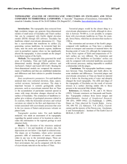
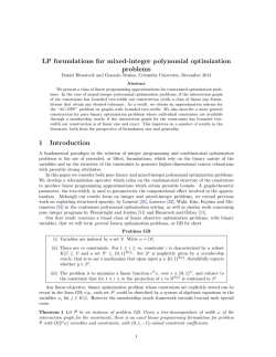

![arXiv:1501.07424v1 [math.LO] 29 Jan 2015](http://s2.esdocs.com/store/data/000457199_1-c519b33964b71d2972f4fe1f35ca3766-250x500.png)
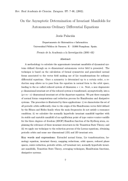
© Copyright 2026