Download Report

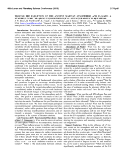
46th Lunar and Planetary Science Conference (2015)
2247.pdf
THE RECESSION OF THE DORSA ARGENTEA FORMATION ICE SHEET: GEOLOGIC EVIDENCE
AND CLIMATE SIMULATIONS. K. E. Scanlon and J. W. Head, Brown University Department of Earth, Environmental and Planetary Sciences, Providence, RI 02912 USA. [email protected]
Introduction: The Dorsa Argentea Formation (DAF)
covers ~1.5 x 106 km2 surrounding and slightly offset
from the south pole of Mars [1-3]. It is characterized by
pitted terrains; branched, sinuous ridges; and plains units
with lobate, rounded margins [1-3]. Topographic, image,
radar, and spectral data have supported the interpretation
[3] that the DAF is the remnant of a large NoachianHesperian ice sheet where abundant melting occurred.
Specifically: (a) sinuous ridges within the deposit are
interpreted as eskers [3, 4] on the basis of their scale,
spacing, cross-sectional shape, sinuosity, branching patterns, branching angles, relationship to underlying topography, and stratigraphic location consistent with subglacial formation [3, 5, 6]; (b) fluvial channels hundreds
of kilometers long head in the DAF and breach impact
craters to create open-basin lake systems on both sides of
the 0° lobe [7, 8]; features in Argentea Planum are also
consistent with a large paleolake in that region [9]; (c)
the steep-sided, flat-topped Sisyphi Montes have been
interpreted as subglacially erupted volcanoes on the basis of their morphology, morphometry, and distribution
[10]; this interpretation has been bolstered by the enhanced concentrations of hydrated sulfates in the edifices
themselves [11, 12]; (d) radar reflectors with the same
footprint as the DAF are consistent with present-day
volatiles in the deposit [13].
In recent years, better image coverage and higher image resolution in the DAF region have become available,
allowing further evaluation of these geomorphological
interpretations. Furthermore, Global Climate Models
have been developed that allow simulations of possible
Late Noachian – Early Hesperian climate conditions on
Mars. We revisit the interpreted fluvial features in the
DAF with higher-resolution data. We also use a suite of
Early Mars climate simulations with the LMD Generic
Climate Model [14, 15] to interpret the distribution of
glaciofluvial landforms and the age and preservation of
esker populations within the DAF in the context of climate change at the Noachian-Hesperian boundary.
Fluid flow properties in subglacial tunnels: The
observation [3, 5, 6] that eskers within the DAF ascend
topographic slopes indicates that the corresponding subglacial channels below the DAF ice sheet were filled
completely by water, such that flow was driven by hydraulic pressure rather than gravity. Fluxes through these
tunnels and the slope of the overlying ice can therefore
be calculated from esker morphometry and distribution.
Fluxes. Banks et al. [16] used a simplified form of
the Darcy-Weisbach equation to estimate the fluxes recorded by eskers in Argyre basin. Following their meth-
ods, assuming a triangular channel cross-section with a
flow depth of 1 or 10 m and a medium sand or coarse
gravel channel bed, and measuring channel width and
bottom slope in large, single-crested eskers among the
Dorsa Argentea, we estimate fluvial discharge on the
order of 1·103 – 1·105 m3s-1. These are comparable to the
values derived for the Argyre eskers [16], as might be
expected if both developed under similar climate conditions. For comparison, typical summer discharges from
beneath the 40 km long Kennicott Glacier in Alaska are
of the order ~102 m3 s-1 [17], but flood discharges of the
order 106 m3 s-1 have occurred beneath Arctic and Antarctic ice sheets in the past [e.g. 18, 19]. We are using
the values and spatial distribution of fluxes measured
from DAF eskers with GCM simulations to constrain the
climate under which the DAF ice sheet receded.
Ice surface slope. Under channel-full conditions, the
vector sum of the topographic gradient along an esker,
the regional dip (multiplied by a constant), and the slope
of the ice surface at the time of esker formation is zero
[20]. To calculate ice slope from present-day topography
and esker paths, we sought well-preserved eskers in regions whose topography is not obscured by glacial debris. Ice slopes calculated over Dorsa Argentea esker
systems fitting these criteria are small, of the order 0.1 m
km-1 throughout. This implies that these eskers formed in
a thick, flat, interior region of the ice sheet rather than
near its edge, where slopes are expected to be steeper.
This scenario is consistent with other evidence [3] for
many eskers in the DAF having formed by basal melting, controlled partially by the thickness of the overlying
ice. It is also consistent with the comparatively young
exposure age of this esker population [21], which suggests that it remained ice-covered longer than populations in other parts of the DAF. Eskers in the Argyre
basin appear to have formed closer to the glacier edge,
allowing Bernhardt et al. [22] to constrain the thickness
(~2 km) of the Argyre paleo ice sheet from calculated ice
slopes. Analysis of other esker populations within the
DAF is ongoing and may allow the DAF paleo ice sheet
thickness to be determined in those regions.
New images of previously described glaciofluvial
features: New images bolster previous interpretations of
glaciofluvial landforms within the DAF. For example,
several of the channels heading in the DAF breach impact craters downstream, creating open-basin lake systems. Ghatan and Head [8] noted fan-shaped deposits at
the mouth of the upstream channel in several of these
crater lakes. HiRISE images reveal horizontal layering in
these deposits, consistent with a sedimentary origin. Ad-
46th Lunar and Planetary Science Conference (2015)
ditionally, several esker systems terminate in the region
interpreted by [9] as a proglacial lake. CTX images reveal that some of these appear to terminate in layered
fan-shaped deposits, typical of eskers terminating in
standing water [e.g. 23].
Global Climate Model simulations: The size and
density of eskers in the DAF indicates that substantial
melting occurred during their construction. The large
size of DAF eskers is easier to explain by terrestrial
standards if a component of the flow through them derived from melting at the glacier surface, propagated
downward to subglacial channels through vertical ice
fractures. The excellent preservation of many eskers,
however, is more consistent with a bottom-up melting
mechanism, where the thickness of the ice sheet allowed
ice to melt at its base despite below-freezing surface
temperatures. In a bottom-up melting scenario, after the
ice had thinned to the point where basal melting could
no longer occur, the cold-based ice would preserve the
underlying landforms [21], whereas top-down melting
would have continued regardless of ice thickness.
Conditions for surface and basal melting. We first
assess the likelihood of basal melting by conducting a
GCM climate simulation with a 1 bar CO2 atmosphere
and 25° spin-axis obliquity. Fastook et al. [24] calculated
that, for ice thickness ~2 km (consistent with minimum
estimates from tuya heights, [10]), annual average temperatures between -75°C (if late Noachian geothermal
fluxes were 65 mW m-2) and -50°C (for 45 mW m-2)
would allow basal melting to occur. Annual average
temperatures in the 1 bar, 25° obliquity climate scenario
are between -57 and -59°C in the regions of the DAF
where eskers are densest. Basal melting could therefore
have occurred even at low obliquity and in a cold early
martian climate, for all but the most conservative geothermal flux. We are currently conducting GCM simulations with higher spin-axis obliquity, as well as a “warm,
wet, early Mars” end-member climate scenario with annual average temperatures above freezing, in order to
constrain the climate conditions under which top-down
melting could have occurred, as well as those under
which the rate and spatial pattern of ice removal could
be consistent with geological observations.
Relationship to age of esker populations. Kress and
Head [21] used buffered crater counting to determine
exposure ages for five esker populations within the DAF.
The youngest populations, i.e. those whose overlying ice
was most recently removed, lie along the 90°W lobe of
the DAF. Populations on the other side of the DAF are
several hundred million years younger. While glacial
flow modeling will be necessary to fully describe the
topography of the DAF ice sheet under plausible paleoclimate conditions, the coldest annual average temperatures at the south pole in our baseline climate scenario
2247.pdf
Figure 1. The Dorsa Argentea Formation. Geologic units shown as
mapped by [2]. White, labeled contours are annual average GCM
temperatures (°K). Eskers mapped in dark blue.
extend along the 90°W lobe (Figure 1). This could have
allowed particularly effective ice preservation in this part
of the deposit. The annual average temperature pattern
also shows a lobe extending along the 0°W meridian,
suggesting that the asymmetry of the DAF may reflect
asymmetry in the former ice sheet.
Conclusions: Our morphemetric analysis of the Dorsa Argentea population of eskers within the DAF suggests that flow through the subglacial channels of the
DAF ice sheet was of the order 103 – 105 m3s-1, and flat
calculated ice sheet topography supports the hypothesis
that these eskers formed due to bottom-up melting in a
thick ice sheet and a cold martian climate. GCM simulations indicate that annual average temperatures could
have supported basal melting in the DAF even for the 1
bar CO2, 25° obliquity scenario. The temperature distribution at the south pole shows cold lobes extending
along the 0° and 90°W meridians, which would have
favored the development of asymmetric polar deposits
recorded by the DAF and a thicker ice cover over the
regions where the most abundant eskers are observed.
References: [1] Tanaka K. L. and Kolb E. J. (2001) Icarus, 154, 3–21.
[2] Tanaka K. L. and Scott D. H. (1987) USGS Misc. Invest. Ser. Map,
I-1802-C. [3] Head J. W. and Pratt S. F. (2001) JGR, 106, 1227512299. [4] Howard A.D. (1981) NASA TM 84211, 286-288. [5] Head J.
W. and Hallet B. (2001) LPSC XXXII, abstract #1366. [6] Head J. W.
and Hallet B. (2001) LPSC XXXII, abstract #1373. [7] Milkovich S. M.
et al. (2002) JGR, 107. [8] Ghatan G. J. and Head J. W. (2004) JGR,
109. [9] Dickson J. L. and Head J. W. (2006) PSS, 54, 251- 272. [10]
Ghatan G. J. and Head J. W. (2002) JGR, 107. [11] Wray J. J. et al.
(2009) Geology, 37, 1043-1046. [12] Ackiss S. E. and Wray J. J.
(2014) Icarus, 243, 311–324. [13] Plaut J. J. et al. (2007) LPSC
XXXVIII, abstract #2144. [14] Wordsworth R. et al. (2013) Icarus, 222,
1-19. [15] Forget F. et al. (2013) Icarus, 222, 81–99. [16] Banks M. E.
et al. (2009) JGR, 114, E09003. [17] Anderson S. P. et al. (2003)
Chem. Geol., 202, 297–312. [18] Shaw J. (1989) Geology, 17, 853–
856. [19] Lewis A. R. et al. (2006) Geology, 34, 513–516. [20] Shreve
R. L. (1985) Quaternary Res., 23, 27–37. [21] Kress, A.K., and J. W.
Head (2014) PSS, in press. [22] Bernhardt H. et al. (2013) PSS, 85,
261–278. [23] Brennand T. A. (2000) Geomorphology, 32, 263-293.
[24] Fastook J.L. et al. (2012) Icarus, 219, 25-40.