1. Art and Diseño

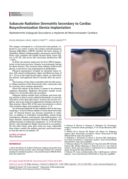
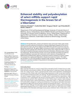
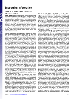
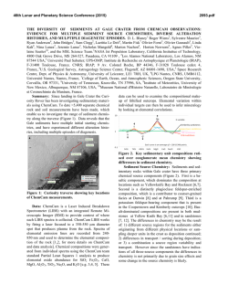
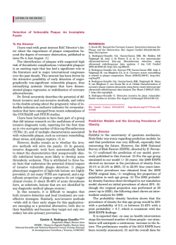
RESEARCH ARTICLE
elifesciences.org
Experimentally guided models reveal
replication principles that shape the
mutation distribution of RNA viruses
Michael B Schulte1,2†, Jeremy A Draghi3†, Joshua B Plotkin3, Raul Andino2*
Tetrad Graduate Program, University of California, San Francisco, San Francisco,
United States; 2Department of Microbiology and Immunology, University of
California, San Francisco, San Francisco, United States; 3Department of Biology,
University of Pennsylvania, Philadelphia, United States
1
Abstract Life history theory posits that the sequence and timing of events in an organism's
lifespan are fine-tuned by evolution to maximize the production of viable offspring. In a virus,
a life history strategy is largely manifested in its replication mode. Here, we develop a stochastic
mathematical model to infer the replication mode shaping the structure and mutation distribution
of a poliovirus population in an intact single infected cell. We measure production of RNA and
poliovirus particles through the infection cycle, and use these data to infer the parameters of our
model. We find that on average the viral progeny produced from each cell are approximately five
generations removed from the infecting virus. Multiple generations within a single cell infection
provide opportunities for significant accumulation of mutations per viral genome and for
intracellular selection.
DOI: 10.7554/eLife.03753.001
*For correspondence: raul.
[email protected]
These authors contributed
equally to this work
†
Competing interests: The
authors declare that no
competing interests exist.
Funding: See page 16
Received: 22 June 2014
Accepted: 31 December 2014
Published: 30 January 2015
Reviewing editor: Stephen P
Goffs, Howard Hughes Medical
Institute, Columbia University,
United States
Copyright Schulte et al. This
article is distributed under the
terms of the Creative Commons
Attribution License, which
permits unrestricted use and
redistribution provided that the
original author and source are
credited.
Introduction
RNA viruses are excellent models for evolution. They replicate quickly and have extremely high mutation rates, orders of magnitude greater than those of most DNA-based life forms (Drake, 1993). While
this combination of traits creates the potential for rapid adaptation, it necessitates a life history
strategy that balances the need for explosive, exponential growth with the requirement to maintain
genomic integrity. The life history strategies of viruses are largely reflected by their mode of intracellular replication. Two classic replication modes have been described for single-stranded RNA viruses:
the ‘stamping machine’ mode (Stent, 1963) and the ‘geometric replication’ mode (Luria, 1951). In the
stamping machine mode (SM), templates made from the original infecting genomes are used for the
production of all progeny genomes. In the geometric replication mode (GR), newly made progeny
genomes are used to create further templates for additional rounds of replication within a single cellular infection cycle (Figure 1). Progeny produced from stamping machine replication are all a single
generation away from the parental strand whereas progeny generated from geometric growth represent a distribution of generations from the parental strand, often resulting in a fractional mean number
of generations (see Figure 1). The iterative nature of GR creates branched genealogies that allow for
expansive exploration of sequence space and results in a mutation distribution that differs from the
SM mode (Luria, 1951). Recent studies with population-genetic models (Draghi et al., 2010) and RNA
enzyme populations (Hayden et al., 2011) have shown that differences in the distribution of mutants
can significantly impact the adaptability of a population. Recent studies with poliovirus (PV) have also
demonstrated that mutational differences within a population can have dramatic effects on pathogenicity (Pfeiffer and Kirkegaard, 2005; Vignuzzi et al., 2006) as well as fitness, virulence, and robustness (Lauring et al., 2012).
Schulte et al. eLife 2015;4:e03753. DOI: 10.7554/eLife.03753
1 of 18
Research article
Genomics and evolutionary biology | Microbiology and infectious disease
eLife digest Viruses with genetic information made up of molecules of RNA can multiply
quickly, but not very accurately. This means that many errors, or mutations, occur when the RNA is
copied to create new viruses. The advantage of this rapid, but mistake-filled, RNA replication
process is that some of the mutations will be beneficial to the virus. This allows viruses to rapidly
evolve, for example, to develop resistance against drugs.
The poliovirus is an RNA virus that can cause paralysis and death in humans. To prevent such
infections, scientists have extensively studied the poliovirus and have developed effective vaccines
against it that have eliminated the virus from all but a few countries. Because so much is known
about the poliovirus and because it has a very simple structure, scientists continue to use the
poliovirus as a model to study virus behavior.
One unknown aspect of the poliovirus' behavior is how it replicates after invading a cell. Are all
of its RNA copies made from the original viral RNA that first infected the cell, in what is known as a
‘stamping machine’ model? Or do the new copies of the RNA also get copied themselves in a
‘geometric replication mode’ that increases the likelihood of mutations and enables the virus to
evolve more rapidly?
Viral RNA molecules are copied by one of the virus's own proteins and so before the viral RNA
can be replicated, it must first be translated to form viral proteins. When and where replication
begins depends on the concentration of translated proteins around the RNA and so replication
tends to begin in particular areas of the cell at different times. Schulte, Draghi et al. used
mathematical modeling to create computer simulations of the number of polioviruses in a cell that
take into account these time and space constraints. By including random elements in the model, the
simulated behavior more accurately follows experimentally recorded data than previously used
models.
The results of the model led Schulte, Draghi et al. to conclude that the poliovirus replicates by
the ‘geometric mode’; as new copies of the poliovirus RNA are made, each copy goes on to make
more copies. This means that in a single infected cell there are multiple generations of RNA, and
each generation may undergo distinct mutations that are passed on to the next set of RNA copies.
In fact, Schulte, Draghi et al. found that the average virus released from an infected cell is the
great-great-great-granddaughter of the original virus that infected the cell. With so many different
generations of virus coexisting in a cell, there are a lot of opportunities for new genetic
combinations to occur and for viruses to evolve new abilities.
DOI: 10.7554/eLife.03753.002
Poliovirus' simple genomic architecture and medical importance have made it one of the most
extensively studied viruses (Racaniello, 2006). However, despite decades of mechanistic studies and
recent revelations of the importance of population structures, the replication mode and resulting
mutation distribution have yet to be determined. PV therefore proves an excellent candidate for the
rigorous construction of a computational model of virus replication to predict population structure and
mutation distribution. A major feature of PV intracellular dynamics is that the genome participates in
multiple reactions: translation, replication, and encapsidation. Its 7.5 kb genome contains a single
open reading frame, which encodes 7 nonstructural proteins and 4 capsid proteins. Translation produces a single polyprotein, which is cleaved into individual functional viral proteins. Replication of the
positive-sense genome by the virus-encoded RNA-dependent RNA polymerase produces a negativesense strand, which is used as a template for further genome synthesis. Evidence suggests that the
initial, infecting positive-sense genomes must be translated before they can replicate (Novak and
Kirkegaard, 1994). The switch from translation to replication appears to be dependent on the concentration of a viral protein product, 3CD, which stimulates a transition from a linear, translating RNA
to a noncovalently associated ‘circular’ RNA competent for replication (Gamarnik and Andino, 1998,
2000; Herold and Andino, 2001). Encapsidation is thought to result from protein–protein associations of capsid pentamers with the RNA replication machinery and protein–RNA association of capsid
pentamers with viral RNA (Pfister et al., 1992; Nugent and Kirkegaard, 1995; Liu et al., 2010). Actively
replicating genomes are preferentially encapsidated and packaging is biased to exclude negativesense strands, although the mechanism of this is not understood (Nugent et al., 1999). Although
Schulte et al. eLife 2015;4:e03753. DOI: 10.7554/eLife.03753
2 of 18
Research article
Genomics and evolutionary biology | Microbiology and infectious disease
multiple ribosomes can translate a genome at
the same time and multiple viral polymerases can
replicate a genome at the same time, the processes are mutually exclusive (Gamarnik and
Andino, 1998). Similarly, neither translation nor
replication can occur after a genome is packaged
into a virion.
Several studies have demonstrated that PV
genomes are often localized to the cytosolic surfaces of the endoplasmic reticulum, Golgi bodies,
Figure 1. Illustrations of the genealogies of different
lysosomes, or vesicles derived from these (Schlegel
replication modes. Red dots indicate positive-sense
et al., 1996; Bolten et al., 1998; Cui et al., 2005;
strands. Blue dots indicate negative-sense templates.
Egger and Bienz, 2005; den Boon et al., 2010).
Stamping machine (SM) progeny are one generation
Replication complexes are thought to form on
from the initial infecting genome (left). In an example
these membranes in cis, resulting in a close assoof geometric replication (GR), progeny are an average
of 2.33 generations from the initial infecting genome
ciation of translation products and positive-sense
(right).
genomes (Novak and Kirkegaard, 1994; Egger
DOI: 10.7554/eLife.03753.003
et al., 2000). Compartmentalization of replication
complexes likely accounts for the observation that
many functions of nonstructural proteins cannot
be complemented in trans (Novak and Kirkegaard, 1994; Ansardi et al., 1996). Only capsid proteins,
3CD, and 3D have been demonstrated to trans-complement (Novak and Kirkegaard, 1994; Nugent
et al., 1999; Oh et al., 2009). Taken together, these studies suggest that the essential transitions—
from translation to replication, and from replication to encapsidation—are largely localized and influenced by the dynamics of the molecules in each compartment.
In recent years, modeling approaches have begun to examine the trade-offs that come with having a genome that is a template for both replication and translation (Krakauer and Komarova, 2003;
Regoes et al., 2005; Sardanyés et al., 2009; Thébaud et al., 2010; Martinez et al., 2011). These
studies have raised mechanistic and evolutionary questions about the life cycle of single-stranded,
positive-sense RNA viruses, but most have not produced models that can be directly compared to
data. Several previous models are deterministic in nature (Krakauer and Komarova, 2003; Regoes
et al., 2005; Martinez et al., 2011) and assume a well-mixed, spatially uniform cellular environment
(Krakauer and Komarova, 2003; Regoes et al., 2005; Sardanyés et al., 2009; Thébaud et al., 2010;
Martinez et al., 2011). Experimental evidence suggests that each of these assumptions is problematic
and do not reflect the biological constraints and properties of viral replication. The small numbers of
the critical molecules that initiate an infection suggest that a stochastic model would more accurately
describe early reactions and could make distinct predictions from previous deterministic approaches
(Srivastavawz et al., 2002). Often infections begin with relatively few virions that release their
genomes into the cell and continue with the translation of these few initial genomes. Random variation
in the switch from translation to replication is amplified by the subsequent exponential phase of the
infection, and this amplification is likely to bias the mean dynamics of a set of infections. Indeed, recent
single-cell studies demonstrated the significant impact of stochastic effects on poliovirus infections
(Schulte and Andino, 2014).
Here, we have developed a stochastic simulation model in which we compartmentalize reactions
in an effort to accurately describe intracellular dynamics in both space and time. Additionally, rather
than fixing each parameter on an estimated value, an approach used by previous models, we use an
Approximate Bayesian Computation approach to fit our parameters from temporal quantitative data.
We find that by combining stochasticity and spatial structure, our model reflects and describes the
population dynamics and structure of the viral population during an infection cycle more accurately
than previous models.
Fitting our model to RNA abundances over time, we find that poliovirus follows the geometric replication mode: multiple iterative generations of genomic replication produce progeny virus. Posterior
parameter fits indicate that progeny of a single cellular infection are approximately five generations
away from the initial, infecting genomes. This replication mode produces populations with expansive,
branched genealogies, creating the dramatic potential for the exploration of sequence space, as well
as creating the potential for intracellular selection among related mutant genomes.
Schulte et al. eLife 2015;4:e03753. DOI: 10.7554/eLife.03753
3 of 18
Research article
Genomics and evolutionary biology | Microbiology and infectious disease
Results
Inference of replication parameters
We used temporal, quantitative RT-PCR data of both positive-sense genomes and negative-sense
strands to estimate the free parameters in our model. The role of each parameter in poliovirus replication and in the mathematics of our model are diagrammed in Figure 2 and described in detail in the
‘Materials and methods’. We chose to use measurements of positive- and negative-sense RNA at
multiple time points for three multiplicities of infection (1, 10, and 100), as well as measurements of
virion numbers at multiple times for MOI 10; this amounted to 27 measured means, with three data
points for each mean. Strand-specific qRT-PCR was performed to quantify positive-sense and negative-sense poliovirus RNA against in vitro transcribed standard RNAs of each sense (Burrill et al.,
2013). Along with cell counts, this allowed for temporal measurements of the average positivesense and negative-sense poliovirus RNA copies per cell. Negative-sense RNA was not detectable
until 2 hr post infection for MOIs 10 and 100 and 3 hr post infection for MOI 1. Positive-sense RNA
was clearly quantifiable for all time points at the MOI 10 and 100 but did not rise above background
levels until 3 hr post infection for MOI 1. Using a newly developed virion immunoprecipitation assay
(Burrill et al., 2013), we observed de novo virion assembly between 2 hr and 3 hr post infection.
Along with total positive-sense RNA measurements from this time course, we obtained a percentage
of genomes encapsidated in quadruplicate at 3 hr, 4 hr, and 5 hr post infection. Figure 3 illustrates
this data alongside projections from inferred parameters from the second round of SMC (see
Figure 3—source data 1).
The relatively high number of data dimensions, combined with the computationally intensive and
highly stochastic nature of our simulations, made a traditional maximum likelihood approach impractical. Instead, we turned to Approximate Bayesian Computation, using as our summary statistic the
sum of the squared deviations of the average simulated RNA concentrations (and average fraction of
virions for MOI 10) from their corresponding empirical means. This algorithm produces progressively
more accurate estimates of each parameter over several rounds; Figure 4—figure supplement 1
illustrates that, for most parameters, round one restricts the credible range of each parameter in
Figure 2. The replication cycle of poliovirus as represented in our model. Numbered steps correspond to sections
and equations in the ‘Materials and methods’.
DOI: 10.7554/eLife.03753.004
Schulte et al. eLife 2015;4:e03753. DOI: 10.7554/eLife.03753
4 of 18
Research article
Genomics and evolutionary biology | Microbiology and infectious disease
Figure 3. Projected mean abundances of positive-sense RNA (solid line simulations vs filled circle experimental measurements), negative-sense RNA
(dashed line simulations vs hollow circle experimental measurements) and virions (orange dotted line simulations vs star experimental measurements;
measured only for MOI = 10). Each row represents a different example parameter set (see ‘Results’); each line is the mean of 20 individual cell simulations, and the means of five sets of 20 replicate simulations are plotted in each panel. Parameter values are given in Figure 3—source data 1.
DOI: 10.7554/eLife.03753.005
The following source data and figure supplement are available for figure 3:
Source data 1. ‘Best’ parameter set used in Figure 3—figure supplement 1, and Figure 4—figure supplement 4.
DOI: 10.7554/eLife.03753.006
Figure supplement 1. Distribution of virions in 10,000 replicates for simulations with (points) and without (line) a deterministic threshold for waiting
times (see ‘Materials and methods’).
DOI: 10.7554/eLife.03753.007
comparison to the flat prior and round two leads to further focusing. The data appear to be uninformative for at least one parameter, cpack; a second parameter, commax, appears to be poorly constrained
by the comparison to MOI = 10 in round one, but somewhat constrained by the broader measurement
against all three MOIs in round two. Round two also appears to significantly move the mode of two
other parameters, ccom and c3A.
Figure 4—figure supplement 1 indicates that ABC inference informed the values of nine of our ten
parameters, but these marginal parameter distributions alone do not capture correlations between
parameter values. Figure 4—figure supplement 2 shows evidence of significant correlations, and
Schulte et al. eLife 2015;4:e03753. DOI: 10.7554/eLife.03753
5 of 18
Research article
Genomics and evolutionary biology | Microbiology and infectious disease
Figure 4—figure supplement 3 shows that parameter sets drawn from the marginal distributions in
Figure 4—figure supplement 1 (i.e., uncorrelated parameter values) do a poor job of matching the
data. While not unexpected, these significant correlations require that we work directly with the sampled parameter sets arising from our inference process, which is the approach we take below.
Each parameter in the posterior is supported over a significant range of possibilities. This remaining
uncertainty reflects two factors: the data may be insufficient to determine each parameter, and the
inference process may not have fully exploited the inferential power of the data. We took several
approaches to quantify the sufficiency of the data and the effectiveness of the inference process. First,
we measured the mean error of parameter sets when compared to the data for each multiplicity of
infection independently; we asked if performance at one MOI predicted performance at the other
two. If so, the dimensionality of our data would be effectively lower than we had initially assumed.
Surprisingly, pairwise correlations between mean error at one MOI and another were very weak:
Spearman's rho is 0.031 for MOIs 1 and 10, −0.092 for MOIs 1 and 100, and 0.129 for MOIs 10 and
100. This suggests that measurements at each MOI are contributing distinct information to our inference process.
Second, we determined the sensitivity of our measure of model ‘fit’ to variation in each of the
parameters. This analysis, described in detail in the ‘Materials and methods’, showed that the data
significantly informed the values of eight of ten of the parameters (Figure 4—figure supplement 4).
We also performed a separate validation analysis which attempted to infer the replication phenotype, g , from mock data simulated from parameter sets drawn from our prior distribution. As
described more fully in the ‘Materials and methods’, this exercise confirms that the data and method
are adequate to infer the trait of interest, albeit with some degree of inaccuracy (Figure 4—figure
supplement 5).
Finally, we examine the fit between the data and the mean dynamics of inferred parameter sets.
Figure 3 shows that the inferred parameter sets generally capture the information in the RNA and
virion data, although some parameter sets deviate consistently from the data for some values.
Variability among replicate sets of twenty single-cell simulations is substantial, correlated across a
time series, and greatest for the smallest MOI. Further inferential effort could improve either the
accuracy of the mean predicted dynamics or the precision of replicate simulation dynamics, though
Figure 3 suggests that such improvements could only be modest. This variability is expected due to
the stochastic nature of the simulations, and it may better reflect the biological noise of the infection
(Schulte and Andino, 2014).
Predicted replication dynamics
Figure 4 shows the inferred posterior distribution of g , the mean number of generations for a packaged virion based on two rounds of inference with measured RNA and virion abundances. This distribution is plotted for MOI = 10; the predicted values at MOI = 1 and MOI = 100 are very similar and
highly correlated (weighted means: MOI = 1, 4.96; MOI = 10, 5.06; MOI = 100, 4.85; Spearman's rho
(unweighted): MOI 1 and 10, 0.92; MOI 1 and 100, 0.85; MOI 10 and 100, 0.96). While this distribution
does show substantial variance, it is strongly inconsistent with a ‘stamping machine’ mode of replication, which would have a g near one.
To explore the robustness of this inference, we compared the predicted dynamics of the model to
an additional type of data: the fraction of positive-sense RNA molecules translating at each time
point. We fractionated infected cell lysates and quantified positive-sense RNAs in monosome and
polysome fractions relative to total positive-sense RNA copies. These data render a percentage of
genomes associated with translation machinery and provide an additional set of data to evaluate the
parameter sets produced by SMC. When measured at an MOI of 10 at 1, 2, 3, 4, and 5 hr post infection, the majority of positive-sense RNAs appeared to be associating with translation machinery, consistently averaging near 85%. Many of the inferred parameter sets are consistent with the measured
values but a substantial fraction is clearly inconsistent (Figure 4—figure supplement 6). The summed
squared error of the translating fractions is also correlated with g (Figure 4—figure supplement 7).
To estimate how these new data inform our prediction of g , we calculated a weighting factor based
on the relative rank of the summed squared error of translating fractions, such that the parameter set
with the best fit was assigned a weight of 1, the next a weight of 1134/1135, etc. Reweighting the
distribution of g by this additional factor produced the distribution shown in Figure 4; the mean g
shifts from 5.06 to 4.78.
Schulte et al. eLife 2015;4:e03753. DOI: 10.7554/eLife.03753
6 of 18
Research article
Genomics and evolutionary biology | Microbiology and infectious disease
Figure 4. Left: posterior distribution of the mean number of generations of replication ( g ). Right: distribution
reweighted by the fit of predicted fractions of translating positive-sense RNA to empirical measurements.
DOI: 10.7554/eLife.03753.008
The following figure supplements are available for figure 4:
Figure supplement 1. Prior and posterior distributions after each of two rounds of inference by Approximate
Bayesian Computation.
DOI: 10.7554/eLife.03753.009
Figure supplement 2. Correlations between parameters in the round two posterior.
DOI: 10.7554/eLife.03753.010
Figure supplement 3. Log of total error for inferred, weighted parameter sets in round two (solid) vs 1000 sets
assembled from parameter values drawn independently from the weighted posterior (dotted).
DOI: 10.7554/eLife.03753.011
Figure supplement 4. Goodness-of-fit (1/[1 + mean error]) of highly replicated simulations for MOI = 10 and the
‘best’ inferred parameter set.
DOI: 10.7554/eLife.03753.012
Figure supplement 5. Inference results from three validation experiments.
DOI: 10.7554/eLife.03753.013
Figure supplement 6. Histograms of the projected fraction of positive-sense RNA undergoing translation for the
mean simulated dynamics of each parameter set, compared to empirical measurements (orange dots).
DOI: 10.7554/eLife.03753.014
Figure supplement 7. Summed squared error (SSE) of fraction of translating positive-sense RNA for all
1135 parameter sets, plotted against g at MOI = 10.
DOI: 10.7554/eLife.03753.015
Predicting the distribution of mutations
We simulated mutation and selection during infections to understand how replication dynamics shape
the distribution of mutation frequencies among virions. To illustrate how mutant frequencies depended
on g , we chose two parameter sets with values of g at the low and high end of the range supported
by the posteriors in Figure 4 and included the ‘best’ parameter set as a representative of the more
common values of g . Mutation frequencies for these parameter sets (‘best’, ‘low’, and ‘high’—see
Figure 3—source data 1) are plotted in Figure 5A for a range of mutants that have a diminished rate
of replication relative to the wild type. We chose to model this particular type of deficiency because
we expected that replication deficits would directly affect the growth and packaging of the mutants.
We observed that deficits in a different trait, the rate of complex formation, were effectively invisible
to intracellular selection (the frequency of a mutation with an 80% reduction in complex formation was
estimated to be reduced by 0.6–4.6% compared to a neutral mutation in the ‘best’ parameter set); we
Schulte et al. eLife 2015;4:e03753. DOI: 10.7554/eLife.03753
7 of 18
Research article
Genomics and evolutionary biology | Microbiology and infectious disease
Figure 5. Left: mean mutation frequencies for three parameter sets (‘low’, g = 3.94; ‘best’, g = 4.65; ‘high’,
g = 5.76). Mutation rate is 2 × 10−5 per replication event; ‘relative replication rate’ reflects the reduced probability
of a mutant template to replicate, relative to an unmutated strand. Grey lines indicate the expected mean for each
parameter set with no selection (deficit of zero); the black line shows the mutation rate in one replication step, and
therefore the expected frequency when mutants cannot replicate. Bars indicate 95% confidence intervals. Right:
distributions of g of progeny from single cell infections for three parameter sets (‘low’, g = 3.94; ‘best’, g = 4.65;
‘high’, g = 5.76).
DOI: 10.7554/eLife.03753.016
expect that mutations in traits like the rate of translation would also be complemented by the wildtype phenotype and so would not experience significant selection during the infection in which they
arose.
Several distinct features of mutation in this model are evident from Figure 5A. Mutation frequency does not decrease linearly as intracellular selection approaches its maximal value; the
curve results from the fact that mutant genomes that are immediately packaged are not subject
to selection, while the contribution of rare, early mutants to average mutation frequency may
be reduced by multiple rounds of intracellular selection. Knowing g and the mutation rate
allows us to directly calculate the fate of neutral or very unfit mutations, but estimating the frequency of mutations of intermediate fitness requires additional simulations using our model.
A third feature is the sizable confidence intervals relative to the number of infections sampled
(10 million for each point). This high variability reflects the large contribution of very rare mutations that arise early in an infection and can contribute 1000s of mutant virions, especially when
selection is weak.
The effect of these rare, early mutations in the overall mutant distribution can be seen as a departure from a Poisson process. To remove a potential confounding variation in burst size, we compare
the distribution of mutations from infections within 10% of the median burst size and calculate a
Poisson expectation for a median-sized burst with the same expected frequency. For the ‘best’ parameter set, median infections produced many more bursts with no copies of a given mutation (79.4% vs
22.5% for the Poisson), but also many more bursts with five or more copies of the mutant (8% vs 1.82%
for the Poisson; n = 51,365).
The distribution of the number of generations between progeny virions and initial infecting
genomes is displayed for three parameter sets (‘best’, ‘low’, and ‘high’—see Figure 3—source data 1)
in Figure 5B. Only a very small percentage of progeny are produced via a single genomic replication
cycle. Although all three parameter sets have means close to five generations, the distributions show
a portion of the progeny virions representing up to 10 generations between the infecting genotypes
and packaged virions within a single cellular infection.
Schulte et al. eLife 2015;4:e03753. DOI: 10.7554/eLife.03753
8 of 18
Research article
Genomics and evolutionary biology | Microbiology and infectious disease
Discussion
The intracellular replication mode of a virus strongly influences the frequency and distribution of mutations among progeny, which shape the long-term behavior of an infecting population (Vignuzzi et al.,
2006; Lauring et al., 2012). Due to the complex nature of intracellular dynamics, assessing the mode
of replication of viruses is a difficult task (but see Chao et al., 2002). Here, we built on decades of
mechanistic studies and recent modeling efforts to construct a stochastic computational model coupled with new Bayesian inference methods. We combined these mathematical and computational
techniques with accurate temporal data to produce a detailed picture of viral infection. We found that
positive- and negative-sense RNA measurements made across multiple MOIs, along with quantitative
data on virion packaging, are sufficient to infer that poliovirus replication occurs in several layers of
intermediate replication, in contrast to the oft-assumed ‘stamping machine’ model. The implications
of the inferred geometric replication mode are as follows: (1) error rates per-replication are considerably lower than measured rates from full-replication-cycle in vivo studies, (2) for a given viral polymerase error rate, mutation will progressively accumulate in both genome and anti-genome RNAs,
which should result in a more accentuated departure from the master sequence, allowing a better
exploration of the available sequence space during a single infection cycle, and (3) there exists a significant potential for intracellular selection and competition among related genomes, even in infections initiated by only a single genome.
Accurate estimates of viral mutation rates are essential for studying viral evolution and have crucial
practical applications in drug and vaccine design. While estimates of mutation rates exist for nearly
two dozen viruses, estimates of replication modes exist for only a few (Sanjuan et al., 2010). Calculating
per-replication event mutation rates from observed mutant frequencies is not possible, or even meaningful, without knowledge of the replication mode. Thus, estimates of poliovirus per-replication
event mutation rates can vary over 10-fold depending on the assumed replication mode (Drake,
1993; Sanjuan et al., 2010). By inferring the mode of replication, we have been able to link estimates of per-replication event mutation rates to published mutant frequencies. The most extensive
poliovirus mutant frequency data set estimated an average mutant frequency of 2 × 10−4 (Acevedo
et al., 2014). Using our inferred value of approximately five intracellular generations, we calculate a
per-replication event mutation rate of 2 × 10−4/5 × 2 = 2 × 10−5, which is in agreement with the average
estimates of poliovirus mutation rates calculated in vivo from lethal mutation frequencies (Acevedo
et al., 2014). Rates of specific types of mutations, such as transversions and transitions, could each
be inferred from their mutation frequencies by the same approach. Our inference of five intracellular generations is also in line with previous inferences of replication mode using the Luria-Delbruck
fluctuation test null-class method (Sanjuan et al., 2010). However, our results highlight some limitations for inferring mutation rates from frequencies: intracellular selection may strongly affect mutation frequencies, and the strong stochastic nature of virus replication appears to deeply modulate
minor allele distribution, which in turn will result in imprecise estimates of the expected frequency.
In particular, assuming that mutation frequency can be modeled as a Poisson process will lead to
inappropriate confidence in measured frequencies. As a consequence, multiple empirical mutation
frequencies measurements will be required to obtain a more precise determination of true mutation
frequencies.
The branched genealogy inferred in our study implies the potential for significant amounts of intracellular complementation, selection, and competition between mutant genomes, even in infections
initiated by a single genome (Novak and Kirkegaard, 1994; Turner and Chao, 1999; Vignuzzi et al.,
2006). Figure 5A demonstrates the extent to which the frequency of a mutation can be skewed by
negative selection during the course of an infection. On the other hand, a mutational event that
occurred early in replication and conveyed an intracellular replication advantage could potentially give
rise to hundreds or thousands of descendant virions in a single generation. If the mutation distribution
data in Figure 5B were displayed as a tree (as in Figure 1), it would contain over 7000 terminal nodes,
too many to resolve in a figure. Hence, the apparent potential for mutant interactions is vast. These
results suggest that the evolutionary fate of mutations may depend strongly on their intracellular competitive ability, even when multiplicities of infection are low. Additionally, studies that rely on bottlenecks to reduce selection in viral mutation studies (e.g., de la Peña et al., 2000) may be allowing more
selection than anticipated. Future population dynamics studies should consider the implications of the
intracellular expansion of mutant phenotypes.
Schulte et al. eLife 2015;4:e03753. DOI: 10.7554/eLife.03753
9 of 18
Research article
Genomics and evolutionary biology | Microbiology and infectious disease
Virus infections are normally depicted as deterministic processes that follow a stereotypical path
from infection to progeny production and death of the infected cell. However, experimental data show
that some infected cells produce few progeny while others produce large populations of progeny
(Schulte and Andino, 2014). These observations support the notion that stochasticity is an important
factor shaping the outcome of infection. By combining accurate experimental measurements with a
stochastic model of viral replication, we have obtained a realistic description of how the molecular
events driving the life cycle of the virus govern the outcome of infection in each cell.
A significant benefit of computational modeling is that the information learned in the empirical
process of the development of a model can yield important insights in the biologic processes under
study. For example, our initial attempts to fit temporal strand measurement data were unable to match
the sharp transition to exponential growth seen in the data. Only after removing the requirement for
positive-sense genomes to be translated before becoming replication-competent was our model
flexible enough to rapidly create templates for exponential replication. While Novak and Kirkegaard
(1994) demonstrate a requirement of the initial, infecting genomes to be translated before replication
can occur, their data did not implicate that all genomes produced at any time during infection must
be translated before replicating. Our study suggests that newly synthesized positive-sense genomes
may or may not disperse to nucleate new replication complexes within a single cellular infection, allowing us to model intracellular dynamics in a novel way by permitting a portion of newly made positivesense strands to immediately act as templates for replication without the requirement of translation.
Our model succeeds in describing many experimentally observed features of viral replication and is
an excellent staging point for future and more accurate models of viral replication and evolution. With
the realistic benefits of stochasticity, compartmentalized reactions, and parameters inferred from
quantitative, temporal data, it acts as a baseline intracellular viral replication algorithm. More quantitative data, including data on the formation and number of replication compartments, would further
inform the model. Potential additions of intracellular selection, complementation, and recombination parameters would allow population evolution studies to explore intracellular dynamics with more
precision than previous approaches. The ultimate goal is to generate a comprehensive model incorporating mechanistic replication dynamics learned from virology with selection and complementation
dynamics learned from population genetics. This tool could be very powerful for informing future
therapeutic and preventative strategies.
Materials and methods
Experimental procedures
Cells and viruses
HeLaS3 cells (ATCC CCL-2.2) were maintained in 50% DMEM/50% F-12 medium supplemented
with 10% newborn calf serum, 100 U/ml penicillin, 100 U/ml streptomycin, and 2 mM glutamine
(Invitrogen). Poliovirus Mahoney type I genomic RNA was generated from in vitro transcription
of prib(+)XpAlong. To generate virus, 20 µg of RNA was electroporated into 4 × 106 HeLaS3 cells in
a 4-mm cuvette with the following pulse: 300 V, 24 Ω, 1000 µF. The resulting virus was passaged at
high multiplicity of infection (MOI ∼1–10) three times then subjected to ultracentrifugation through a
30% sucrose cushion.
Infections
Four wells of HeLaS3 cells in 12-well plates were washed, trypsinized, and counted twice each on a
hemocytometer then averaged to determine cell count. To synchronize infections, plates were placed
on ice, cells were washed with cold serum-free media and infected at MOIs 1, 10, and 100. Plates were
incubated at 4°C for 30 min with rocking every 10 min to adhere virus. After removal of the inoculum,
cells were washed 2× with warm serum-free media. Cells were then incubated at 37°C in 2% serum
media until harvest. To harvest, plates were frozen at −70°C.
RNA extraction, reverse transcription (RT), and qPCR
Plates were thawed on ice and refrozen at −70°C 3×. RNA was extracted via the PureLink RNA
Micro Kit (Life Technologies) according to the manufacturer's instructions. cDNA was synthesized from
total RNA using SuperScript III Reverse Transcriptase (Life Technologies) and 125 nM strand-specific
RT primer (+strand_RT: 5′-GGCCGTCATGGTGGCGAATAATGTGATGGATCCGGGGGTAGCG-3′;
Schulte et al. eLife 2015;4:e03753. DOI: 10.7554/eLife.03753
10 of 18
Research article
Genomics and evolutionary biology | Microbiology and infectious disease
-strand_RT: 5′-GGCCGTCATGGTGGCGAATAACATGGCAGCCCCGGAACAGG-3′) in a 5-µl reaction.
Separate RT reactions for positive and negative-strand RNAs were performed for each sample.
RT products were treated with 0.5 units of Exonuclease I (Fermentas) to remove excess RT primer
prior to qPCR. Strand-specific qPCR was based on a published protocol (Burrill et al., 2013). cDNAs
were analyzed by qPCR using 2× SYBR FAST Master Mix (Kapa Biosystems), 200 nM strandspecific qPCR primer (+strand_For: 5′-CATGGCAGCCCCGGAACAGG-3′; -strand_Rev: 5′-TGTGAT
GGATCCGGGGGTAGCG-3′), and 200 nM Tag primer (5′-GGCCGTCATGGTGGCGAATAA-3′) in a
10-µl reaction. A 10× dilution series of in vitro transcribed positive- and negative-strand RNA standards was run alongside experimental samples and used to construct a standard curve.
Virion immunoprecipitation
Lysates from MOI 10 infections were homogenized with a final concentration of 0.06% NP-40.
Immunoprecipitation was performed using Protein A-coated Dynabeads and anti-poliovirus antibody
according to a published protocol (Burrill et al., 2013).
Sucrose gradients
HeLaS3 cells were infected for 1, 2, 3, 4, and 5 hr at an MOI of 10 in 15-cm dishes then simultaneously treated with 100 µg/ml cycloheximide (CHX) for 2 min at 37°C. Cells were washed with
PBS+CHX and lysed with 0.5% NP-40 lysis buffer containing CHX on ice for 20 min. Cell debris was
pelleted in a table-top centrifuge at 2000 rpm for 10 min at 4°C, then nuclei were pelleted at
9000 rpm for 10 min at 4°C. Cell lysates were loaded on a 10–50% sucrose gradient containing CHX
and ultracentrifuged at 35,000 rpm for 3 hr. Fractions were collected on a Biocomp Gradient Station
with a BioRad Econo UV Monitor. Fractions were pooled based on the spectrophotographic trace
into two fractions (ribonucleoprotein and monosome/polysome fractions), RNA was extracted and
subjected to qRT-PCR.
Modeling replication
Outline of stochastic simulation
We developed a stochastic simulation model that tracks discrete abundances of poliovirus molecular
species within a cell and simulates individual reactions. This model is based on the Gillespie algorithm
(Gillespie, 1976). In this model, stochastic events, such as the production, decay, or transformation of
molecular species, are represented by reaction rates. Each rate can depend on x, the vector of abundances of all species in the system. Given an initial state x0 at t = 0, the algorithm proceeds for a set
duration (tmax) as follows:
a. Sum the rates of all reactions 1..n in the system; rtotal = ∑ i =1ri ( x ).
n
b. Draw the time until the next event, Δt, from an exponential distribution with a mean of rtotal.
c. Advance to time t + Δt.
d. Choose which event occurred by drawing from a multinomial with probabilities ri(x)/rtotal.
e. Change x to reflect the chosen event.
f. If t < tmax, return to step (a).
Similar to Hensel et al. (2009), we have modified the basic Gillespie algorithm to balance accuracy
and speed. When the rtotal is below a threshold (1000 events/min), we draw exponential times as
described above; when it is above this threshold, we use the inverse of the rate—the expected time—
as our interval between reactions. Figure 3—figure supplemental 1 shows that this approximation
delivers accurate results for the best (lowest error) inferred parameter set. This procedure allows us to
efficiently generate stochastic realizations of replication, translation, and other reactions unfolding in
a single infected cell, based on a system of equations that describes each essential reaction in the
poliovirus life cycle. Results from many replicate simulations are then averaged to predict the dynamics
across a population of infected cells.
Figure 2 depicts the events in poliovirus replications captured quantitatively by our model, each of
which is described in detail below.
Binding (step 1)
We assume that the number of virions that bind to, and subsequently infect, a cell is Poisson distributed with a mean equal to the multiplicity of infection (MOI). This formulation assumes that bound
Schulte et al. eLife 2015;4:e03753. DOI: 10.7554/eLife.03753
11 of 18
Research article
Genomics and evolutionary biology | Microbiology and infectious disease
virions do not interfere with the binding of additional virions during the period of infection. We denote
these coated positive-sense RNA genomes at RNA+initial; their distribution is therefore:
+
RNAinitial
~Poisson (MOI ).
(1)
Uncoating (step 2)
A quantitative description of uncoating was derived from the data presented in Brandenberg et al.
(2007); based on these data, we choose the two-parameter gamma distribution to model stochasticity
in this process. To account for differences in experimental protocols, we excluded the t = 0 measurement from Brandenberg et al.'s data and, taking the t = 8 min measurement as the starting point,
fit the gamma distribution to the average cumulative measurements. Using the optim() function in
R, we obtained an estimate of 0.678 for the shape parameter, and 0.02 for the rate parameter (n = 28,
R2 ≈ 0.92). Each of the RNA+initial molecules transitions to a translationally competent, linear-form positive-sense RNA, RNA+lin, after a waiting time, tuncoat, drawn from Equation 2.
t uncoat ~Gamma(0.02, 0.678).
(2)
Translation (step 3)
Translation is the first role of positive-sense genomes in a cell, and it continues as the primary role
throughout the infection. Because poliovirus translates a single polyprotein, we assume that all protein
products are produced at equal rates based upon a single rate-constant of initiation. We also assume
that poliovirus genomes, and not cellular factors, are rate-limiting, and neglect the delay between
the initiation of translation and the appearance of the protein products. With these assumptions,
translation can be modeled as a first-order equation with a single parameter, ctrans, yielding a rate of
translation:
+ 
rtrans = c trans RNAlin
 .
(3)
Here, and throughout the model, we consider these rates to describe Poisson processes, rather
than changes in continuously valued quantities. Square brackets are used to indicate the concentration
per cell, or abundance, of each molecular species. We track three protein products of translation: the
procapsid units, which we abbreviate CAP, and protein products 3A and 3CD. Based on evidence from
complementation experiments, we assume that CAP units and 3A diffuse freely, while 3CD accumulates within complexes with translating genomes (Novak and Kirkegaard, 1994; Ansardi et al., 1996;
Nugent et al., 1999). Equation 3 applies to translation of both complex-associated and free genomes.
Global abundances of CAP and 3A are tracked, while abundances of 3CD are tracked individually for
each replication complex. 3CD arising from the translation of free genomes is ignored.
Replication complex formation (step 4)
We assume that two events must happen before a translating positive-sense strand can replicate:
it must attach to a membrane, representing nucleation of a replication complex, and it must circularize through association with 3CD (Gamarnik and Andino, 1998; Herold and Andino, 2001). Once
a strand associates with a membrane, we consider that it has formed a complex, and assume that all
subsequent translation events will add to the local concentration of 3CD. We model this first step by
introducing a rate, rcompart, at which the RNA+lin species forms complexes. We also assume that the viral
protein product 3A facilitates this complex formation (Hsu et al., 2010). Finally, we assume that complex formation is limited by the supply for suitable membrane, which limits the number of possible
complexes in a cell to commax (Guinea and Carrasco, 1990). We therefore introduce a first-order reaction scaled by the number of existing complexes, com, the maximum, commax, and the concentration
of the protein 3A:

[com] 
[3A ].
rcom = c com 1–
 commax 
(4)
While other viral and cellular proteins are involved in complex formation, we assume that their
influence is adequately represented by tracking the concentration of 3A. We also represent the
Schulte et al. eLife 2015;4:e03753. DOI: 10.7554/eLife.03753
12 of 18
Research article
Genomics and evolutionary biology | Microbiology and infectious disease
consumption of some number of 3A molecules in the formation of each complex by a parameter c3A.
If insufficient 3A is available upon complex formation, newly translated proteins are consumed by the
existing complex until c3A have been allocated. Therefore, we are assuming that 3A binding is cooperative, and that incomplete complexes have much higher affinity for 3A than does the reaction to form
a new complex.
Circularization (step 5)
We model circularization—the transition of a positive-sense genome from a linear, translating molecule to a noncovalently associated circularized molecule competent for replication—as a first-order
reaction driven by the concentration of the viral protein 3CD in each complex (indexed by i).
i
rcirc
= c circ [3CD ]i .
(5)
This formulation reflects experimental data supporting the direct role of 3CD in circularization
(Gamarnik and Andino, 1998; Herold and Andino, 2001), and the low rate of rescue of 3CD-deficient
strains by complementation in trans (Novak and Kirkegaard, 1994).
Replication (step 6)
We distinguish replication rates for positive and negative strand synthesis with separate rate constants
crep+ and crep−. We ignore polymerase concentrations and instead assume that both types of replication
are first-order reactions modified by a common cellular resource limit. This limitation is parameterized
by repmax, the maximum number of replication events per cell permitted by some limited resource and
implemented with a running counter, rep, of synthesized RNAs. We also assume that per-capita replication does not differ between replication complexes, allowing us to write a mass-action equation for
both replication reactions.

rep 
+ 

rrep+ = c rep+ RNAcirc
 1– rep  .
max
(6a)

rep 
– 

rrep – = c rep – RNAcirc
 1– rep .
max
(6b)
Note that rrep+ measures the rate at which replication is initiated on positive-sense templates, producing negative-sense strands, and similarly, rrep− measures the rate of positive-strand production.
We allowed newly synthesized positive-sense genomes one of three fates: (1) associate with capsid
protomers and become encapsidated, (2) diffuse into the cytoplasm where they can translate and
potentially create new, independent compartments, or (3) remain in the complex in which they were
generated and act as templates for further RNA replication. We assume that positive-sense genomes
that remain in the complex are immediately competent for replication. We were unable to fit the sharp
transition to exponential growth seen in our strand measurement data without allowing for this third
option. Allowing newly synthesized positive-sense genomes to remain in the complex and act immediately as replication templates is consistent with previous reports indicating a coupling between
translation and replication as we still require initial, infecting genomes to be translated before transitioning to replication (Novak and Kirkegaard, 1994). Negative-sense strands also stay in the complex
in which they were produced and are immediately competent for replication.
We assume that only the positive-sense replication-competent form is packaged (Ansardi et al.,
1996, but see; Liu et al., 2010), and that, following Nugent et al. (1999), genomes can only be packaged as they are synthesized from a negative-sense strand. We therefore first determine whether the
newly synthesized positive-sense strand is packaged; then, for unpackaged genomes, we calculate
whether they remain in the replication complex.
Packaging (step 7)
We assume that the rate of initiation of packaging is proportional to the global concentration of a
virus-derived protein product, CAP, representing capsid protomers. These protomers form pentamers,
of which 12 are required for each capsid; each packaging event therefore consumes 60 units of CAP.
To account for the evidence that deficiencies in capsid proteins can be complemented in trans, we
Schulte et al. eLife 2015;4:e03753. DOI: 10.7554/eLife.03753
13 of 18
Research article
Genomics and evolutionary biology | Microbiology and infectious disease
allowed capsid proteins to diffuse freely throughout the cell. As with 3A molecules and complex formation, if a packaging event begins when the global abundance of CAP is less than 60, then further
packaging is halted until this deficit is filled.
Using the approximation that each available CAP molecule independently contributes to the probability of packaging, we derive the probability that a newly synthesized positive-sense strand is packaged to be:
ppack = 1– e
– c pack [CAP ]
(7)
.
Positive strand dispersal (step 8)
The probability of a newly synthesized positive-sense strand to remain within its replication complex,
assuming it was not packaged, is given by the parameter cstay. The total probability is therefore:
pstay = c stay (1– ppack ) .
(8)
Replication phenotype
Our primary goal is to infer the number of replication cycles between the infecting and the progeny
virions. Defining a complete replication cycle to include both copying to a negative-sense strand, then
back to a positive-sense strand, we label the mean of this value g . The principal purpose of this mean
is to link the mutation rate of replication to the mean mutation frequency in the progeny population,
so the appropriate measure is to average over virions, not infected cells. For k replicate simulations,
let ni represent the number of progeny produced by each replicate i, and gij represent the number of
replication cycles in the ancestry of each virion j in replicate i; then we calculate g as follows.
∑ ∑
g=
∑ n
k
ni
g
j =1 ij
i =1
k
i =1 i
(9)
.
Parameter inference
Inference method
We chose to implement a version of Approximate Bayesian computation called Sequential Monte
Carlo (Sisson et al., 2007; Toni et al., 2009; Beaumont, 2010; Csilléry et al., 2010; Lopes and
Beaumont, 2010; Toni and Stumpf, 2010). This method consists of several rounds of parameter
selection which form successively better approximations of the posterior distribution. In each round x,
a population of size nx parameters sets is generated iteratively by choosing a parameter set from the
preceding round x − 1, perturbing its values, then accepting or discarding the new parameter set
based on the distance of its measured summary statistic from the summary statistic representing the
data. Parameter sets with distances less than εx are accepted; a diminishing series of thresholds,
ε1 > ε2 > ε3, etc, progressively focuses the search on those parameter values that best match the data.
In round 1, parameter sets are drawn from the prior distributions; this first round is therefore identical
to the basic rejection algorithm, but with a fairly large ε1 to reduce computation time.
The advantage of searching for better parameter sets near previously identified good values is
a much higher frequency of acceptance, and therefore much less computational time. However, the
parameters accepted in later rounds are then biased toward common values in the previous rounds.
The SMC algorithm removes this bias by weighting the selection of parameter sets against those that
are most similar to their parent round, and toward those that resemble the prior distribution. Let Kσ(θa, θb)
represent the probability of perturbing θa into θb with a Gaussian kernel of standard deviation σ, wxi
represent the weight of parameter set i in round x, θxij represent the value of parameter j in set i of
round x, and π(θ) represent the prior probability of θ. Then, for round two and later, we calculate these
importance weights as in Equation 10 (adapted from Toni et al., 2009).
∑
∑
10
w x ,i =
Schulte et al. eLife 2015;4:e03753. DOI: 10.7554/eLife.03753
∑
nx –1
w x –1,k
k =1
π (θ x ,i , j )
j =1
10
K
(θ x –1,k , j ,θ x ,i , j )
j =1 σ x –1, j
.
(10)
14 of 18
Research article
Genomics and evolutionary biology | Microbiology and infectious disease
Beaumont (2010) suggests that the Gaussian perturbations applied to each proposed parameter
set should be scaled with regard to the variance in that parameter in the previous round. In practice,
we identified a trade-off based on the scaling of these perturbations; smaller perturbations lead to
increased acceptance rates but more positively skewed importance weights; because the weighting
of each accepted parameter set is normalized relative to the highest observed importance weight,
this strong skew effectively dilutes the inferential power of the analysis. We found that using the standard deviation of each parameter as the standard deviation for the perturbation balanced this tradeoff adequately for our model: the weights of the 1135 sampled parameter sets had an entropy of
10.01 bits, compared to a maximal value of 10.15 bits. This high entropy confirms that any remaining
skew in the importance weights does not severely diminish the effective sample size.
Implementing this method requires several additional choices: the shapes of prior distributions, the
number of rounds, the values of ε, and the number of replicates, n, to perform for each evaluation of
the model. This last decision turned out to be crucial; inferring based on the mean of a larger number
of replicates (n ≥ 1000) tended to select parameter sets with highly variable behavior. Reducing n led
to a higher rate of parameter set rejection but more biologically plausible dynamics. A simple explanation for this pattern is that a number of parameter sets produce acceptable mean behavior, but
differ in the degree of stochastic variation around that mean in a way that does not reflect measured
stochastic variation (Schulte and Andino, 2014). We therefore chose to accept parameter sets that
passed a given ε for multiple, sequential sets of n replicates. For round 1, one thousand parameters
sets were accepted based on five sets of n = 20 replicates at MOI = 10 only with ε = 12. For round 2,
1135 parameters sets were accepted based on five sets of n = 20 replicates at MOI = 1 with ε = 16,
five sets of n = 20 replicates at MOI = 10 with ε = 12, and five sets of n = 20 replicates at MOI = 100
with ε = 7. Thresholds for round 2 were calibrated to achieve an acceptance rate of about 1 in 10,000.
Approximate Bayesian computation uses summary statistics to judge the fit of model predictions to
data. We chose to compute the sum squared error of the log of the mean abundances of positive- and
negative-sense RNA, and the log ratio of positive-sense RNA in capsids to the total positive pool. This
produced a single summary statistic that captured the total error of the predictions from a particular
parameter set. Using the natural logs for each data point effectively weights each deviation by its relative magnitude, which prevents the large absolute size of errors at later time steps from dominating
the error measurement.
To aid in visual exploration of the data, we chose five representative parameter sets as follows.
From an initial batch of 513 parameter sets, we chose the 50 sets with the overall lowest error. From
these, we sampled sets of five at random and calculated the summed pairwise distance in parameter
space of those five sets from each other. To adjust for the different scales and uncertainties in each
parameter, the contribution of each parameter to the distance measure was divided by its standard
deviation over the whole set of 513 values. These summed distances provided a metric of the parameter diversity captured in a choice of five parameter sets; we examined one thousand randomly drawn
sets of five and chose the set with the highest summed distance. These five parameter sets are shown
in Figure 3—source data 1.
Method validation
To test the effectiveness of the inference process and the adequacy of our data, we chose parameter
sets from the prior, produced simulated data from these parameter sets, and then performed the
sequential Monte Carlo method described above. We chose three sets of parameters based on two
criteria: representation of a high diversity of the replication phenotype, g , and biological plausibility.
We achieved these criteria by sampling the prior, measuring g and the mean number of virions at
MOI = 10, and choosing three parameter sets than spanned the range of g and produced a number
of virions similar to the empirically measured value.
For each parameter set, we measured RNA abundances and, for MOI = 10, virion abundances with
10,000 replicate simulations. These data were then treated exactly as the empirical data were handled;
the log of the averages was used to measure error in the Bayesian inference procedure described
above. At least one thousand accepted parameter sets were collected for both inference rounds
(except in one case in which fast convergence and lengthy computation times made round two unnecessary and computationally costly).
The mean RNA abundances for MOI = 10 and the inference results are plotted in Figure 4—figure
supplement 5. In each case, the inference process produced a narrow posterior, relative to the prior,
Schulte et al. eLife 2015;4:e03753. DOI: 10.7554/eLife.03753
15 of 18
Research article
Genomics and evolutionary biology | Microbiology and infectious disease
with clear similarity to the actual value of g for each starting parameter set. However, the mean of the
final posterior fails to perfectly match the true value in all three cases. Also, the second round of inference, which more than doubles the amount of data used to assess goodness-of-fit, achieved little in
these validation experiments. The error thresholds (values of ε) used here may have been too permissive to achieve complete convergence to the correct value. Nonetheless, these experiments show that
our statistical method, when combined with the types and quantities of data we have available, can
produce a reliable inference.
Sensitivity analysis
To further investigate if the parameter values identified by ABC minimize the error in predicted RNA
and virion dynamics, we explored the sensitivity of mean error to variation in each parameter for a
single parameter set (‘Best’ in Figure 3—source data 1). As before, error was assessed by comparing
the log of the mean RNA and virion abundances to empirical data for sets of 20 simulations. 500 trials
of 20 simulations each at each MOI were averaged to produce a high-resolution estimate of true
deviation from the data. These results are plotted as 1/(1 + mean error) to show an intuitive goodnessof-fit measure, where high values indicate similarity to the data. Figure 4—figure supplement 4 shows
that the ‘best’ parameter set is at or near a local maximum for goodness-of-fit for eight of ten parameters; the effects of the remaining two parameters, cpack and commax, appear to be minimal for this
parameter set. These results suggest that convergence of the posterior distributions is linked to the
sensitivity of the model to each parameter, which supports the effectiveness of the ABC algorithm.
Additional information
Funding
Funder
Grant reference number
Author
National Institute of Allergy and
Infectious Diseases
R01 AI36178
Michael B Schulte,
Raul Andino
National Institute of Allergy and
Infectious Diseases
R01 AI40085
Michael B Schulte,
Raul Andino
Defense Advanced Research
Projects Agency
BAA-10-93
Michael B Schulte,
Raul Andino
Burroughs Wellcome Fund
JBP
Joshua B Plotkin
David and Lucile Packard Foundation JBP
Joshua B Plotkin
U.S. Department of the Interior
D12AP00025
Joshua B Plotkin
Army Research Office
W911NF-12-1-0552
Joshua B Plotkin
The funders had no role in study design, data collection and interpretation, or the
decision to submit the work for publication.
Author contributions
MBS, JAD, Conception and design, Acquisition of data, Analysis and interpretation of data, Drafting
or revising the article; JBP, RA, Conception and design, Analysis and interpretation of data, Drafting
or revising the article
Additional files
Supplementary file
• Source code 1. Poliovirus replication mathematical model-code. Contains custom software used for
simulations throughout this article.
DOI: 10.7554/eLife.03753.017
References
Acevedo A, Brodsky L, Andino R. 2014. Mutational and fitness landscapes of an RNA virus revealed through
population sequencing. Nature 505:686–690. doi: 10.1038/nature12861.
Schulte et al. eLife 2015;4:e03753. DOI: 10.7554/eLife.03753
16 of 18
Research article
Genomics and evolutionary biology | Microbiology and infectious disease
Ansardi DC, Porter DC, Anderson MJ, Morrow CD. 1996. Poliovirus assembly and encapsidation of genomic
RNA. Advances in Virus Research 46:1–68. doi: 10.1016/S0065-3527(08)60069-X.
Baltimore D, Girard M, Darnell J. 1966. Aspects of the synthesis of poliovirus RNA and the formation of virus
particles. Virology 29:179–189. doi: 10.1016/0042-6822(66)90024-9.
Beaumont MA. 2010. Approximate Bayesian Computation in evolution and ecology. Annual Review of Ecology,
Evolution, and Systematics 41:379–406. doi: 10.1146/annurev-ecolsys-102209-144621.
Bolten R, Egger D, Gosert R, Schaub G, Landmann L, Bienz K. 1998. Intracellular localization of poliovirus
plus- and minus-strand RNA visualized by strand-specific fluorescent in situ hybridization. Journal of Virology
72:8578–8585.
Brandenberg B, Lee LY, Lakadamyali M, Rust MJ, Zhuang X, Hogle JM. 2007. Imaging poliovirus entry in live
cells. PLOS Biology 5:e183. doi: 10.1371/journal.pbio.0050183.
Burrill CP, Strings VR, Schulte MB, Andino R. 2013. Poliovirus: generation and characterization of mutants.
Current Protocols in Microbiology Chapter 15: Unit 15H.2. doi: 10.1002/9780471729259.mc15h02s29.
Chao L, Rang CU, Wong LE. 2002. The distribution of spontaneous mutants and inferences about the replication
mode of the RNA bacteriophage phi6. Journal of Virology 76:3276–3281. doi: 10.1128/JVI.76.7.3276-3281.2002.
Csilléry K, Blum MG, Gaggiotti OE, François O. 2010. Approximate bayesian computation (ABC) in practice.
Trends in Ecology & Evolution 25:410–418. doi: 10.1016/j.tree.2010.04.001.
Cui ZQ, Zhang ZP, Zhang XE, Wen JK, Zhou YF, Xie WH. 2005. Visualizing the dynamic behavior of poliovirus
plus-strand RNA in living host cells. Nucleic Acids Research 33:3245–3252. doi: 10.1093/nar/gki629.
de la Peña M, Elena SF, Moya A. 2000. Effect of deleterious mutation-accumulation on the fitness of RNA
bacteriophage MS2. Evolution 54:686–691. doi: 10.1111/j.0014-3820.2000.tb00069.x.
den Boon JA, Diaz A, Ahlquist P. 2010. Cytoplasmic viral replication complexes. Cell Host & Microbe 8:77–85.
doi: 10.1016/j.chom.2010.06.010.
Draghi JA, Parsons TL, Wagner GP, Plotkin JB. 2010. Mutational robustness can facilitate adaptation. Nature
463:353–355. doi: 10.1038/nature08694.
Drake JW. 1993. Rates of spontaneous mutation among RNA viruses. Proceedings of the National Academy of
Sciences of USA 90:4171–4175. doi: 10.1073/pnas.90.9.4171.
Egger D, Bienz K. 2005. Intracellular location and translocation of silent and active poliovirus replication
complexes. The Journal of General Virology 86:707–718. doi: 10.1099/vir.0.80442-0.
Egger D, Teterina N, Ehrenfeld E, Bienz K. 2000. Formation of the poliovirus replication complex requires
coupled viral translation, vesicle production, and viral RNA synthesis. Journal of Virology 74:6570–6580.
doi: 10.1128/JVI.74.14.6570-6580.2000.
Gamarnik AV, Andino R. 1998. Switch from translation to RNA replication in a positive-stranded RNA virus.
Genes & Development 12:2293–2304. doi: 10.1101/gad.12.15.2293.
Garmarnik AV, Andino R. 2000. Interactions of viral protein 3CD and poly(rC) binding protein with the
5' untranslated region of the poliovirus genome. Journal of Virology 74:2219–2226. doi: 10.1128/JVI.74.5.
2219-2226.2000.
Gillespie DT. 1976. General method for numerically simulating stochastic time evolution of coupled chemicalreactions. Journal of Computational Physics 22:403–434. doi: 10.1016/0021-9991(76)90041-3.
Guinea R, Carrasco L. 1990. Phospholipid biosynthesis and poliovirus genome replication, two coupled phenomena. The EMBO Journal 9:2011–2016.
Hayden EJ, Ferrada E, Wagner A. 2011. Cryptic genetic variation promotes rapid evolutionary adaptation in an
RNA enzyme. Nature 474:92–95. doi: 10.1038/nature10083.
Hensel SC, Rawlings JB, Yin J. 2009. Stochastic kinetic modeling of vesicular stomatitis virus intracellular growth.
Bulletin of Mathematical Biology 71:1671–1692. doi: 10.1007/s11538-009-9419-5.
Herold J, Andino R. 2001. Poliovirus RNA replication requires genome circularization through a protein-protein
bridge. Molecular Cell 7:581–591. doi: 10.1016/S1097-2765(01)00205-2.
Hsu NY, Ilnytska O, Belov G, Santiana M, Chen YH, Takvorian PM, Pau C, van der Schaar H, Kaushik-Basu N, Balla T,
Cameron CE, Ehrenfeld E, van Kuppeveld FJ, Altan-Bonnet N. 2010. Viral reorganization of the secretory
pathway generates distinct organelles for RNA replication. Cell 141:799–811. doi: 10.1016/j.cell.2010.03.050.
Krakauer DC, Komarova NL. 2003. Levels of selection in positive-strand virus dynamics. Journal of Evolutionary
Biology 16:64–73. doi: 10.1046/j.1420-9101.2003.00481.x.
Lauring AS, Acevedo A, Cooper SB, Andino R. 2012. Codon usage determines the mutational robustness,
evolutionary capacity, and virulence of an RNA virus. Cell Host & Microbe 12:623–632. doi: 10.1016/j.
chom.2012.10.008.
Liu Y, Wang C, Mueller S, Paul AV, Wimmer E, Jiang P. 2010. Direct interaction between two viral proteins, the
nonstructural protein 2C and the capsid protein VP3, is required for enterovirus morphogenesis. PLOS
Pathogens 6:e1001066. doi: 10.1371/journal.ppat.1001066.
Lopes JS, Beaumont MA. 2010. ABC: a useful Bayesian tool for the analysis of population data. Infection,
Genetics and Evolution 10:826–833. doi: 10.1016/j.meegid.2009.10.010.
Luria S. 1951. The frequency distribution of spontaneous bacteriophage mutants as evidence for the exponential
rate of phage reproduction. Cold Spring Harbor Symposia on Quantitative Biology 16:463–470. doi: 10.1101/
SQB.1951.016.01.033.
Martinez F, Sardanyés J, Elena SF, J-A Daròs. 2011. Dynamics of a plant RNA virus intracellular accumulation:
stamping machine vs. geometric replication. Genetics 188:637–646. doi: 10.1534/genetics.111.129114.
Novak JE, Kirkegaard K. 1994. Coupling between genome translation and replication in an RNA virus. Genes &
Development 8:1726–1737. doi: 10.1101/gad.8.14.1726.
Schulte et al. eLife 2015;4:e03753. DOI: 10.7554/eLife.03753
17 of 18
Research article
Genomics and evolutionary biology | Microbiology and infectious disease
Nugent CI, Johnson KL, Sarnow P, Kirkegaard K. 1999. Functional coupling between replication and packaging of
poliovirus replicon RNA. Journal of Virology 73:427–435.
Nugent CI, Kirkegaard K. 1995. RNA binding properties of poliovirus subviral particles. Journal of Virology
69:13–22.
Oh HS, Pathak HB, Goodfellow IG, Arnold JJ, Cameron CE. 2009. Insight into poliovirus genome replication and
encapsidation obtained from studies of 3B-3C cleavage site mutants. Journal of Virology 83:9370–9387.
doi: 10.1128/JVI.02076-08.
Pfeiffer JK, Kirkegaard K. 2005. Increased fidelity reduces poliovirus fitness and virulence under selective
pressure in mice. PLOS Pathogens 1:e11. doi: 10.1371/journal.ppat.0010011.
Pfister T, Pasamontes L, Troxler M, Egger D, Bienz K. 1992. Immunocytochemical localization of capsidrelated particles in subcellular fractions of poliovirus-infected cells. Virology 188:676–684. doi: 10.1016/
0042-6822(92)90522-Q.
Racaniello VR. 2006. One hundred years of poliovirus pathogenesis. Virology 344:9–16. doi: 10.1016/j.
virol.2005.09.015.
Regoes RR, Crotty S, Antia R, Tanaka MM. 2005. Optimal replication of poliovirus within cells. The American
Naturalist 165:364–373. doi: 10.1086/428295.
Sanjuán R, Nebot MR, Chirico N, Mansky LM, Belshaw R. 2010. Viral mutation rates. Journal of Virology 84:
9733–9748. doi: 10.1128/JVI.00694-10.
Sardanyés J, Solé RV, Elena SF. 2009. Replication mode and landscape topology differentially affect RNA virus
mutational load and robustness. Journal of Virology 83:12579–12589. doi: 10.1128/JVI.00767-09.
Schlegel A, Giddings TH Jr, Ladinsky MS, Kirkegaard K. 1996. Cellular origin and ultrastructure of membranes
induced during poliovirus infection. Journal of Virology 70:6576–6588.
Schulte MB, Andino R. 2014. Single-cell analysis uncovers extensive biological noise in poliovirus replication.
Journal of Virology 88:6205–6212. doi: 10.1128/JVI.03539-13.
Sisson SA, Fan Y, Tanaka MM. 2007. Sequential monte carlo without likelihoods. Proceedings of the National
Academy of Sciences of USA 104:1760–1765. doi: 10.1073/pnas.0607208104.
Srivastavawz R, You L, Summers J, Yin J. 2002. Stochastic vs. deterministic modeling of intracellular viral kinetics.
Journal of Theoretical Biology 218:309–321. doi: 10.1006/jtbi.2002.3078.
Stent GS. 1963. Molecular Biology of Bacterial Viruses. San Francisco, Calif: W H Freeman and Company.
Thébaud G, Chadoeuf J, Morelli MJ, McCauley JW, Haydon DT. 2010. The relationship between mutation
frequency and replication strategy in positive-sense single-stranded RNA viruses. Proceedings Biological
Sciences/ the Royal Society 277:809–817. doi: 10.1098/rspb.2009.1247.
Toni T, Welch D, Strelkowa N, Ipsen A, Stumpf MP. 2009. Approximate Bayesian computation scheme for
parameter inference and model selection in dynamical systems. Journal of the Royal Society, Interface 6:
187–202. doi: 10.1098/rsif.2008.0172.
Toni T, Stumpf MP. 2010. Simulation-based model selection for dynamical systems in systems and population
biology. Bioinformatics 26:104–110. doi: 10.1093/bioinformatics/btp619.
Turner PE, Chao L. 1999. Prisoner's dilemma in an RNA virus. Nature 398:441–443. doi: 10.1038/18913.
Vignuzzi M, Stone JK, Arnold JJ, Cameron CE, Andino R. 2006. Quasispecies diversity determines pathogenesis
through cooperative interactions in a viral population. Nature 439:344–348. doi: 10.1038/nature04388.
Schulte et al. eLife 2015;4:e03753. DOI: 10.7554/eLife.03753
18 of 18