1. Art and Diseño

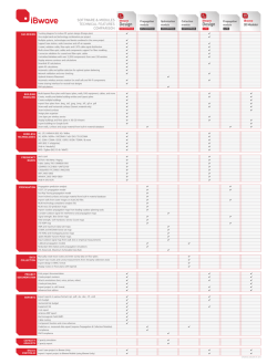
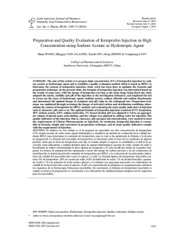
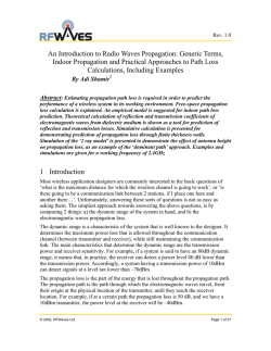
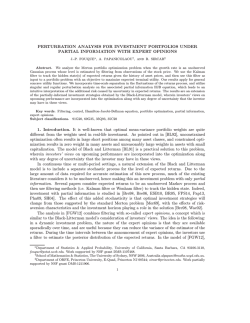
PROPANE: An Environment for Examining the Propagation
of Errors in Software
Martin Hiller
[email protected]
Arshad Jhumka
[email protected]
Neeraj Suri
[email protected]
Department of Computer Engineering
Chalmers University of Technology
Goteborg,
¨
Sweden
ABSTRACT
In order to produce reliable software, it is important to have knowledge on how faults and errors may affect the software. In particular, designing efficient error detection mechanisms requires not
only knowledge on which types of errors to detect but also the effect these errors may have on the software as well as how they
propagate through the software. This paper presents the Propagation Analysis Environment (PROPANE) which is a tool for profiling and conducting fault injection experiments on software running
on desktop computers. PROPANE supports the injection of both
software faults (by mutation of source code) and data errors (by
manipulating variable and memory contents). PROPANE supports
various error types out-of-the-box and has support for user-defined
error types. For logging, probes are provided for charting the values of variables and memory areas as well as for registering events
during execution of the system under test. PROPANE has a flexible design making it useful for development of a wide range of
software systems, e.g., embedded software, generic software components, or user-level desktop applications. We show examples of
results obtained using PROPANE and how these can guide software
developers to where software error detection and recovery could increase the reliability of the software system.
Keywords
Error Propagation Analysis, Software Reliability, Fault Injection,
Software Development Tools
1.
INTRODUCTION
In order to develop software that functions in a non-harmful
manner in the presence of faults and errors (as defined in [9]), one
requires knowledge of the behavior of the software under these exceptional conditions. In particular, one needs to know how faults
Supported in part by Volvo Research Foundation (FFP-DCN),
NUTEK (1P21-97-4745), Saab, NSF Career CCR 9896321, and
by EC DBench (IST-2000-25425)
Permission to make digital or hard copies of part or all of this work or
personal or classroom use is granted without fee provided that copies are
Permission to make digital or hard copies of all or part of this work for
not
made or
or distributed
for profit
or commercial
copies
personal
classroom use
is granted
without feeadvantage
provided and
thatthat
copies
are
bear
this notice
and the full
citationoron
the first page.
To copy
otherwise,
to
not made
or distributed
for profit
commercial
advantage
and
that copies
republish,
to post
or toonredistribute
to To
lists,
requires
prior
bear this notice
andon
theservers,
full citation
the first page.
copy
otherwise,
to
specific
permission
a fee.
republish,
to post onand/or
servers
or to redistribute to lists, requires prior specific
©
2002 ACM
1-58113-562-9...$5.00
permission
and/or
a fee.
ISSTA 2002 Rome, Italy
Copyright 2002 ACM 1-58113-562-9/02/0007 .…….......$5.00.
and errors propagate to affect the execution of software. Knowing propagation pathways may, for instance, be of great help when
deciding where to place error detection and recovery mechanisms.
Learning about error propagation characteristics of a software
system requires not only that one should be able to inject errors
and monitor the effect these have on system output, but also that
one is able to monitor how these errors are transported through the
system. Thus, high observability is required for these activities.
Ideally, one should be able to observe every individual variable and
data structure in the software.
This paper presents the main features of PROPANE (details are
available in [6]), the Propagation Analysis Environment, which
enables the injection of primarily errors (e.g. erroneous variable
contents) but also faults (e.g. source code defects) into software
running on a desktop computer (currently for Windows NT/2000).
PROPANE supports various ways of probing a system, i.e., tracing
internal variables and events during system operation, as well as
ways of injecting software faults and data errors.
PROPANE can be useful in a number of situations. For instance,
in Component-Based Software Development (CBSD) generic configurable software components are manufactured and assembled to
form an entire system (inspired by the use of generic hardware
components for building hardware systems). These components
are often ported to several different hardware platforms. This limits generalized verification and validation use of tools that focus on
specific hardware configurations. PROPANE on the other hand has
no such limitations as it is does not require any special hardware assistance. Thus, software components may be verified and validated
with PROPANE before porting them to various target hardware.
This argument will of course also be valid for testing embedded
software which in many cases may exist before the hardware platform has been finalized.
We emphasize that PROPANE, through its depiction of error
propagation paths, is primarily designed as a software design aid
with complementary capability of being used in the evaluation of
effectiveness of error handling mechanisms.
The remaining paper is structured as follows: In Section 2 we
describe the target system model for which PROPANE is aimed.
Section 3 describes the PROPANE tool suite and it’s main features.
An example of actual PROPANE usage is shown in Section 4. In
Section 5, we shortly compare PROPANE to some similar tools.
Finally, in Section 6 we summarize this paper.
2. TARGET SYSTEM MODEL
PROPANE aims at modular software, i.e., discrete software functions interacting to deliver the requisite functionality. A module in
81
this context is a generalized software block having possibly multiple inputs and outputs. Modules communicate with each other
in some specified way using varied forms of signaling, e.g., shared
memory, messaging, parameter passing etc., as pertinent to the chosen communication model.
A software block performs computations using the provided inputs to generate the outputs. At the lowest level, such a software
block may be a procedure or a function but could also conceptually
be a basic block or particular code fragment within a procedure or
function (at a finer level of software abstraction). A number of such
modules constitute a system and they are inter-linked via signals,
much like hardware components on a circuit board. Of course, this
system may be seen as a larger component or module in an even
larger system.
Software constructed as such is found in numerous systems–
desktop systems as well as embedded systems. For example, most
applications controlling physical events, e.g. in automotive systems, are traditionally built up as such. Our studies mainly focus
on software developed for embedded systems in consumer products
(high-volume and low-production-cost systems).
The PROPANE environment is designed with a focus on software for single-process user applications on desktop systems. However, this single process may be multi-threaded. The PROPANE injection and logging mechanisms are generic and are provided in a
static C-library, thus allowing for a vast range of applications. For
example, it has been used in experimentally analyzing the propagation of data errors in the software of an embedded control system
simulated on a Windows-based desktop computer [7, 8]. The requirement for using PROPANE is that the language used for the
source code is able to interface with libraries implemented in the C
programming language.
3.
MAIN FEATURES OF PROPANE
This section provides an overview of the main features of the
PROPANE tool suite, how it is structured, and its proposed usage.
3.1 Basic system structure
PROPANE is designed to run on a desktop system and consists
of a suite of tools, namely: the PROPANE Setup Creator (PSC), the
PROPANE Campaign Driver (PCD), the PROPANE Library (PL),
and the PROPANE Data Extractor (PDE). An overview is shown in
Fig. 1.
Target executable
The campaign driver invokes
the target executable to run
experiments
PROPANE Library
PROPANE
Campaign Driver
PCD
User Error
Types
Environment
simulator
PROPANE
Setup Creator
User Error
Triggers
PL
Target software
PROPANE
Data Extractor
PSC
PDE
Setup
files
Log
files
Readout
files
Extracted
data
Figure 1: An overview of PROPANE together with target software and environment simulator
The PL is used by the target system to gain access to the probing and injection functionality of PROPANE and is written in the
C programming language. The PCD is responsible for handling
the actual execution of experiments and is in a sense the main administrator of PROPANE. It has a user interface through which the
user can control and follow the experiments. The PDE may be used
during analysis to extract specific data from the experiment readout
files. The PCD and the PL are integrated with each other, whereas
the PSC and the PDE are stand-alone components of PROPANE.
The environment simulator and target software are provided by the
user. The environment simulator will act as a stimuli generator for
the target software and may be partially controlled by the output
generated by the target software (e.g., as in a control loop). The interactions between these two sub parts of the target executable are
user-defined.
The PSC aids in the creation of setup files needed for controlling
PROPANE during the execution of FI-experiments. Given information regarding errors and faults, probes, injection locations, etc.,
it will generate the requisite description files. The PSC will also
generate description files used by the PDE during analysis.
For each experiment specified in the description files, the PCD
spawns a new process running an executable file containing a complete specification for conducting one experiment. This executable
contains the PL which performs the actual injection of errors and
logging of variables. The executable also has to contain everything
necessary to run the target system and the environment simulator.
During the execution of the experiments, log files and readout
files are created. The log files contain information regarding the
execution of the experiments, i.e., PROPANE performance and behavior information, and does not contain any readout data gathered
from the target software. If the experiment could not be executed
successfully for some reason, the log files provide hints to potential problems. The readout files contain the data obtained by the
inserted probes and the performed injections and are the basis for
subsequent error propagation analysis. The environment simulator
is designed by the user of the PROPANE tool, hence it may or may
not use description files and may or may not create log files and/or
readout files as per user-specified requirements. Also, the format of
the files read and/or written by the environment simulator is userdefined.
The PL requires interfacing to the environment simulator. However, if an environment simulator exists which does not comply
with the interface specifications, a wrapper layer is warranted which
has the PROPANE interface on one side and the environment simulator interface on the other, acting as a translator between the two
components. Thus, the environment simulator need not necessarily
be an integrated part of the target executable.
The PDE will extract traces of the various logged variables and
memory areas and can conduct Golden Run Comparisons (i.e. comparing system traces obtained during injection experiments with
fault/error free reference traces, so called Golden Runs) to detect
whether errors have occurred due to fault injection. Information
regarding propagation will be compiled and presented. Also, intermediate extracted data is stored in special files which can subsequently be used in a customized analysis tools which may take
into account desired experiment specific information and/or aims,
such as coverage estimation of error handling mechanisms, failure
classification or other activities which may be target specific.
3.2 Work process for using PROPANE
The typical work process when using PROPANE can basically
be divided into three main phases, namely: 1) Setup, 2) Injection,
and 3) Analysis (as illustrated in Fig. 2).
Setup phase: In the Setup phase, description files are generated
and the target system is instrumented. The inputs to this phase include the original source code of the target software, information
82
Original
target
software
Fault
and error
data
Usage
profile
data
SETUP
Description files
Instrumented
target
software
INJECTION
Log files
Readout files
ANALYSIS
Results
Figure 2: The basic work process when using PROPANE.
on distribution and nature of faults and/or errors and information
about target system usage. The fault and error information is used
for determining the fault and error sets to be injected in the experiments. The usage information forms the basis for determining the
test cases used during the injections in order to provide the target
system with a realistic operational profile. Instrumentation of the
target system means adding probes for logging variables, memory
areas, and events, as well as with high-level software traps for injecting faults/errors to the source code. At this point, target instrumentation is still a manual task. However, a tool for automatic instrumentation is currently being developed and will be added to the
PROPANE suite. Given basic information about errors and faults,
probes, injection details, etc., PSC generates the required description files for PCD/PL and PDE. The description files contain information on which faults are to be injected, which errors are to be
injected and at which locations, and which test cases are to be used
by the environment simulator during the execution of experiments.
Injection phase: During the Injection phase, the PROPANE
Campaign Driver (PCD) is set up with the description files generated in the Setup phase. The PCD invokes the target executable
as an individual process and generates readout files containing detailed information on the results of the experiments. During the
experiment, the specified faults and/or errors are injected and the
specified variables and events are logged. Log-files are generated
recording the actions of the PROPANE tool itself.
Faults are injected when the corresponding fault-triggers are activated. Fault injection at this level means that a faulty piece of
code is executed instead of the correct piece.
Errors are injected based on the built-in error types, or on userimplemented error types. Thus, it is possible to implement error
models which are not originally included in PROPANE. For example, if some parts of a system work unreliably under extreme
temperatures, a user error type could take this into consideration.
Error-triggers are boolean expressions and an error is injected
when its corresponding error-trigger is evaluated to true. Errortriggers may be based on time, frequency or a probability distribution. In addition to the built-in error-triggers, PROPANE also
supports user-implemented error-triggers. As was the case for user
error types, a user error-trigger may take into account target specific
information, such as system state or the environment. In the example with the temperature-induced error type, a corresponding errortrigger may evaluate to true when the temperature (obtained from
the environment simulator) is below a lower threshold or above an
upper threshold (or both).
Analysis phase: The readout files generated in the Injection
phase are analyzed in the Analysis phase to evaluate metrics for the
target systems. These metrics may include coverage values, propagation information, etc. One aspect of analysis is to compare traces
from two different runs with each other, e.g., compare a golden
run(i.e. a reference run) with an injection run. The PROPANE Data
Extractor compiles propagation information from the readout files
and also generates a set of data-files containing data such as detailed results on Golden Run Comparisons, injection information,
propagation information, etc.
4. EXAMPLE RESULTS GENERATED BY
PROPANE
This section presents example results obtained using PROPANE.
In [7], we used PROPANE on the software of an embedded control system for arresting aircraft on short runways (such as aircraft
carriers). The system aids incoming aircraft to reduce their velocity, eventually bringing them to a complete stop. The structure of
the software is illustrated in Fig. 3. The numbers shown at the inputs and outputs are used for numbering the signals. For instance,
PACNT is input #1 of DIST S, and SetValue is output #2 of CALC.
We used the actual software ported and it to run on a Windowsbased computer. The scheduling is slot-based and non-preemptive.
Thus, from the software viewpoint, there is no difference in running
on the actual hardware or running on a desktop computer.
i
ms_slot_nbr
1
CLOCK
PACNT 1
Rotation
sensor
HW
counter
TIC1
2
DIST_S
TCNT 3
1
1
1
2
mscnt
2
pulscnt
3
1
slow_speed
4
2
stopped
5
CALC
2
3
SetValue
1
Pressure
sensor
ADC 1
PRES_S
1
2
V_REG
1
1
OutValue
PRES_A
1
TOC2
IsValue
Figure 3: SW structure of the example system.
The software is composed of six modules of varying size and input/output signal count. CLOCK provides a clock, mscnt, and a
signal indicating the current execution slot, ms slot nbr. DIST S
receives PACNT and TIC1 from sensors and are used to calculate the distance an aircraft has traveled on the runway, pulscnt.
It also provides two boolean values, slow speed and stopped, i.e.,
if the velocity of the aircraft is below a certain threshold or if it
has stopped. CALC uses mscnt, pulscnt, slow speed and stopped
to calculate SetValue, the preferred value for the system actuators.
PRES S reads the value that is actually being applied by the actuators, ADC, and provides the signal IsValue. V REG uses SetValue
and IsValue to generate OutValue, the output value to the actuators.
The modules attempts to compensate for the difference between
SetValue and IsValue. PRES A uses OutValue to set the actuator
via the hardware register TOC2.
We injected bit-flip errors in each of the signals (one at a time)
and monitored all the signals. Details on the setup and further results of this experiment can be found in [7].
During data analysis, the PDE extracts vital information for the
assessment of error propagation for each individual experiment run
but also for groups of experiments. Due to space limitations, we
will in this paper only show examples of results for groups of ex-
83
1840 errors
PACNT
1840
0/0/20
1120
0/0/20
pulscnt
691
10/10/20
617
1/252/3313
i
307
29/296/3303
SetValue
1275
2/2/2
18
0/0/0
214
10/1361/4030
TOC2
1257
7/10/315
151
10/1358/4020
351
7/96/147
ADC
8
5/5/5
10
88/88/88
292
43/2083/5261
892
109/2081/5932
892
109/2081/5932
mscnt
TCNT
8
2/2/2
10
57/57/57
892
109/2081/5932
292
121/856/2801
307
29/296/3303
1192
138/144/145
IsValue
892
109/2081/5932
617
1/252/3313
slow_speed
292
121/856/2801
76
9/890/2349
TIC1
292
121/856/2801
ms_slot_nbr
292
121/856/2801
351
7/96/147
OutValue
Figure 4: Propagation graph (generated by the dot tool) for errors injected in PACNT.
periments. PDE generates concise information pertaining to the
propagation of the injected errors in the system. For each signal
that is subjected to error injections, a propagation graph and propagation summary will be generated. The PDE stores the propagation
graph in two different file formats: i) dot [2], and ii) GML [4]. As
these formats are common for graph representation, there is a range
of applications that can be used for plotting and manipulating the
propagation graphs. In Fig. 4 we can see the propagation graph for
errors injected into the PACNT in the example system used in this
section. The graph is generated using the dot tool.
The propagation graph illustrates the propagation characteristics
of the errors injected into the signals PACNT. The label on an arc
from one node to another tells how many errors propagated along
this arc (top value), and the minimum, average and maximum propagation times (bottom values) for these errors. The graph shows the
temporal order between errors in different signals. For example, if
we consider the errors detected (during the Golden Run Comparison) in i, we can see that for 1120 of them, there were no errors
detected earlier in other signals (although errors were detected in
pulscnt at the same point in time), whereas for 691 of the detected
errors, there were error detected earlier in pulscnt.
Using the same example experiment as above, we show the generated propagation summary for errors in PACNT in Table 1. The
summary is obtained by collapsing all ingoing arcs of each node in
the propagation graph. Thus, e.g., the summary for i is obtained by
adding its two ingoing arcs in the propagation graph, which gives
us a total of 1811 errors. The propagation times are obtained from
the combined set of propagation times for the errors detected in i.
Table 1: Propagation of errors injected into PACNT.
error count is the number of errors detected using Golden Run Comparison and the error rate is the same information normalized. The
propagation times are all in milliseconds.
Signal
error count
error rate
tmin
tavg
tmax
PACNT
1840
1.000
0
0
0
pulscnt
1840
1.000
0
0
20
i
1811
0.984
0
4
20
OutValue
1275
0.693
1
613
4159
SetValue
1275
0.693
1
613
4159
TOC2
1275
0.693
3
615
4161
ADC
1265
0.688
10
629
4168
IsValue
1202
0.653
155
682
3467
slow speed
769
0.418
0
2004
5890
mscnt
1184
0.643
476
2982
6201
ms slot nbr
1184
0.643
476
2982
6201
TCNT
1184
0.643
476
2982
6201
TIC1
1184
0.643
476
2982
6201
In the summary shown in Table 1 we see the number of errors in
PACNT that caused errors in other signals (count and rate), as well
as the minimum, average and maximum propagation time for these
errors (the rows are ordered according to their average propagation
time). In this particular example we can see that all of the 1840
errors injected into PACNT, propagated to pulscnt with an average
propagation time of 0 ms. 1275 errors made it all the way to the
output signal TOC2 with an average propagation time of 615 ms.
84
From the software structure shown in Fig. 3 we can see that errors
in the signals listed below TOC2 in Table 1 (except slow speed),
must be indirect, since there is no direct path from PACNT. Thus,
errors in this signal must have propagated out of the system into the
environment and then back into the system again.
The results presented give information on how errors propagate
through the system, identifying which modules and signals that
may be in need of special mechanisms for protection against propagating errors. For example, from the results in Table 1 we see that
errors in PACNT mainly propagate through DIST S into CALC
using pulscnt. From the propagation graph in Fig. 4 we see that
propagation into CALC is fast, whereas propagation out of CALC
takes a little longer. Thus, CALC seems to delay the propagation
of errors. We also see that after CALC, error propagation again
is swift. These results would indicate that system reliability could
increase if pulscnt were to be equipped with with EDMs (error detection mechanisms) and ERMs (error recovery mechanisms), as
this would likely break the propagation at an early stage.
These examples demonstrate PROPANE’s capabilities for generating pertinent information for propagation analysis. However,
the level of detail required may generate very large amounts of raw
data. In order to further analyse this raw data (further than done
by the PDE) additional actions can be performed to reduce the raw
data into useful information. We refer the reader to [7, 8], where
details of actual results, as well as two different data analysis frameworks (with different objectives) are described.
5.
OTHER TOOLS
There are other tools for injection of errors and faults, e.g. DEPEND [5], Xception [1], MAFALDA [3], and NFTAPE [10]. DEPEND is aimed at evaluating architectures and thus the granularity
of the obtained results is at the system level (or node level for distributed systems) and thus cannot aid in charting error propagation
at the variable level. Xception is targeted for evaluation of fault tolerance against HW faults and its results are also at the system level.
Also, Xception connects directly to the hardware of a system and
thus has a tight link to the target processor.
The aim of MAFALDA is evaluation of the robustness of microkernels and investigating the effect of software faults and software
errors on the operation of these kernels. This means that the tool is
able to inject at the OS-level. PROPANE is aimed at software at the
USER-level, hence it is not suited for these types of investigations.
However, as far as we know, MAFALDA lacks comprehensive logging facilities for examining the propagation of errors in a microkernel. NFTAPE is, in our opinion, a very versatile tool which can
perform the same investigations PROPANE can. NFTAPE, just like
PROPANE, has support for user-defined injectors as well as userdefined triggers, and is capable of observing the target system at
the variable level. As both tools have support for user-defined injectors, both may be extended to handle physical fault injection as
well as SWIFI. However, NFTAPE is designed to run on a LAN,
and has therefore a separate control host and a target node.
6.
SUMMARY
This paper briefly presents PROPANE, the Propagation Analysis
Environment, which is a software design-stage profiling tool suite
developed for analyzing the propagation and effect of errors in software systems. PROPANE is a desktop environment and contains
support for conducting fault and error injections in target software
systems. The tool also provides support for inserting probes into
the target system enabling the logging of variables and events during injection experiments.
PROPANE is totally target system independent, i.e., it may be
used on any target system provided that one can execute it in a
desktop environment. Also, PROPANE does not require any HW
or OS support and is easily ported to other operating systems (the
current version is available for Windows NT/2000-based computers). As PROPANE is implemented using ANSI C, porting it is
mostly just a question of recompiling for the desired environment.
The injection capabilities include fault injection by mutation of
source code as well as SWIFI-based injection of errors. PROPANE
supports user-defined injectors and triggers which makes it capable
of supporting other injection techniques than SWIFI (for example,
physical fault injection).
PROPANE supports observations down to the variable level, i.e.,
individual variables may be logged during injection experiments.
This enables the detailed examination of error propagation in software and is a valuable help in finding vulnerable software modules
and/or variables.
For analysis, the toolkit contains the PROPANE Data Extractor,
which can perform Golden Run Comparisons for each channel created by a variable in the readout files. The results will be stored
in a text file with a spreadsheet format that is easily imported into
other tools for further analysis. The results from the GRC are also
compiled to show where errors propagate through the system and
how long time it takes.
The PDE can also extract injection information from the readout
files and store this in separate files, and create channel logs for each
individual channel of each individual experiment if a more detailed
analysis or graphical representation is desired. Also, PDE creates
propagation graphs and summaries which visualize the propagation
characteristics of the software system.
To demonstrate the tool we have shown detailed results from an
injection experiment performed on a medium sized embedded control system used for arresting aircraft (similar to the cable-and-hook
systems found on aircraft carriers).
7. REFERENCES
[1] Carreira J., et al., “Xception: A Technique for the
Experimental Evaluation of Dependability in Modern
Computers”, IEEE Trans. on Software Eng., Vol. 24, No. 2,
pp. 125-136, 1998
[2] Information about the tool suite to which dot belongs is
found at http://www.research.att.com/sw/tools/graphviz
[3] Fabre J.-C., et al., “Assessment of COTS Microkernels by
Fault Injection”, Int. IFIP Conf. on Dependable Computing
for Critical Applications, 1999
[4] Information about GML and related tools is found at
http://www.infosun.fmi.uni-passau.de/graphlet/GML
[5] Goswami K.K., et al., “DEPEND: A Simulation-Based
Environment for System Level Dependability Analysis”,
IEEE Trans. on Comp., Vol. 46, No. 1, pp. 60-74, 1997
[6] Hiller M., “A Tool for Examining the Behavior of Faults and
Errors in Software”, TR 00-19, Dept. of CE, Chalmers Univ.,
(available at www.ce.chalmers.se/LDC/DEEDS/), 2000.
[7] Hiller M., et al., “An Approach for Analysing the
Propagation of Data Errors in Software”, Int. Conf. on
Dependable Systems and Networks, pp. 161-170, 2001
[8] Jhumka A., et al., “Assessing Inter-modular Error
Propagation in Distributed Software”, Symp. on Reliable
Distributed Systems, pp. 152-161, 2001
[9] Laprie J.-C. (ed.), “Dependability: Basic Concepts and
Terminology”, Dependable Computing and Fault-Tolerant
Systems series, Vol. 5, Springer-Verlag, 1992
[10] Stott D.T., et. al, “NFTAPE: A Framework for Assessing
Dependability in Distributed Systems with Lightweight Fault
Injectors.”, Int. Computer Performance and Dependability
Symposium, pp. 91-100, 2000
85