1. No category

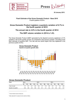
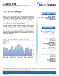
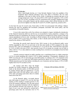
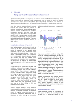
Working Paper
DT/2015/3
Quarterly regional GDP flash
estimates for the Spanish
economy (METCAP model)
Abstract
In this paper we propose a methodology to estimate on a quarterly basis the GDP of the
different regions of Spain, providing quarterly profiles for the annual official observed data.
In this way, the paper offers a new instrument for short-term monitoring that allows the
analysts to quantify the degree of synchronicity among regional business cycles.
Technically, we combine time series models with benchmarking methods to process shortterm monthly and quarterly indicators and to estimate quarterly regional GDPs ensuring
their temporal and transversal consistency with the National Accounts data. The
methodology addresses the issue of non-additivity taking into account explicitly the
transversal constraints imposed by the chain-linked volume indexes used by the National
Accounts and provides an efficient combination of structural as well as short-term
information.
The methodology is illustrated by an application to the Spanish economy, providing realtime quarterly GDP estimates for the period 2000:1 – 2014:4.
Writen by Ángel Cuevasτ and Enrique M. Quilisτ
Revised by Rafa Frutos and Gabriel Perez-Quirós
Approved by José Marín
Key words: balancing, benchmarking, dynamic factor models, national accounts,
regional analysis.
JEL: C53, C43, C82, R11
τ Spanish
Independent Authority for Fiscal Responsibility
We thank A. Abad, J.L. Escrivá, A. Espasa, R. Frutos and G. Pérez-Quirós for their input
at different stages of the project. Any views expressed herein are those of the authors and
not necessarily those of the Spanish Independent Authority for Fiscal Responsibility
La Autoridad Independiente de Responsabilidad Fiscal (AIReF) nace con la misión de velar por el estricto
cumplimiento de los principios de estabilidad presupuestaria y sostenibilidad financiera recogidos en el artículo
135 de la Constitución Española.
Contacto AIReF: C/José Abascal, 2, 2º planta. 28003 Madrid.Tel. +34 917 017 990
Email: [email protected]. Web: www.airef.es
Este documento no refleja necesariamente la posición de la AIReF sobre las materias que contiene. La
documentación puede ser utilizada y reproducida en parte o en su integridad citando su procedencia.
DT/2015/3
Summary
1
Introduction ............................................................................................... 3
2
Data ............................................................................................................ 4
2.1
2.2
2.3
3
Regional accounts ................................................................................ 6
Short-term regional indicators ............................................................... 7
Autonomous regional accounts ............................................................. 9
Econometric approach ............................................................................10
3.1
3.2
3.3
3.4
Processing short-term indicators ..........................................................10
Design of regional GDP trackers using dynamic factor analysis ..........11
Quarterly regional GDPs: initial (unbalanced) estimation .....................16
Quarterly regional GDPs: final (balanced) estimation ..........................18
4
Numerical results: Spanish quarterly regional GDPs. ..........................21
5
Conclusions .............................................................................................23
6
References................................................................................................25
A.
Appendix: short-term regional indicators..............................................28
May 2015
Quarterly regional GDP flash estimates for the Spanish economy
(MEPTCA model)
2
DT/2015/3
1 Introduction
Monitoring economic conditions at the regional level is an important component in the
assessment of the economic state of large and medium size countries as well as for
countries with decentralized administrative systems that allow the application of specific
economic policies. This is clearly the case for Spain: its medium economic size and its
decentralized fiscal system are good reasons to consider explicitly the regional
dimension in the evaluation of its global economic conditions and to do it in a timely
manner.
In addition, fiscal monitoring and forecasting assessment at the regional level is a key
mandate for
the
Independent
Authority for
Fiscal
Responsibility
(Autoridad
Independiente de Responsabilidad Fiscal, AIReF) and this is why we propose in this
paper the use of a modular and transparent system to ascertain the economic conditions
of the Spanish economy at the regional level. In this way, for instance, AIReF can
evaluate the degree of homogeneity of the short-term economic conditions at the
regional level or estimate its own measures of cyclical and structural fiscal conditions for
each region.
The design of the system incorporates the available statistical sources of information at
the structural level as well as at the short-term level, satisfying their consistency by
means of benchmarking techniques (temporal disaggregation and balancing). At the
same time, the system is symmetric in the use of the regional information ensuring, that
all the regions are considered in the same way.
In this paper we propose a methodology to obtain quarterly estimates of the Gross
Domestic Product (GDP) for all the Spanish regions, derived in a consistent way with the
official available data provided by the National Accounts, both Regional Accounts (RA)
and Quarterly National Accounts (QNA). In this way, early (or flash) estimates of
quarterly GDP at the regional level can be released at the same time as the national
GDP. Finally, the methodology ensures that transversal consistency is compliant with
the chain-linking procedures, circumventing its non-additive features in the balancing
step.
May 2015
Quarterly regional GDP flash estimates for the Spanish economy
(MEPTCA model)
3
DT/2015/3
The methodology has three main stages:
1. Processing of the high frequency indicators available at the regional level and
estimation, for each region, of a GDP tracker that combines the available short
term information using dynamic factor analysis.
2. Temporal disaggregation and interpolation of annual regional GDPs using the
corresponding GDP trackers estimated in step 1.
3. Balancing of these initial quarterly estimates in order to ensure transversal
consistency with the national quarterly GDP, preserving at the same time the
temporal consistency achieved in the previous stage.
Our paper relies heavily on Cuevas et al. (2011, 2015), modifying their work in two critical
issues. First, we introduce dynamic factor models to estimate the high-frequency
(quarterly) regional GDP trackers instead of static factor models. In this way, we enrich
the dynamic specification of the models and we obtain a measure of the uncertainty
around the GDP tracker. Second, we expand their set of indicators to take into account
the financial conditions at the regional level.
The paper is organized as follows. The second section describes the available statistical
sources of information used by the system. The third section is devoted to the modeling
approach, going into detail of its main steps. A complete and in depth application of the
methodology using Spanish data appears in section four. The paper ends presenting the
main conclusions and future lines of research.
2 Data
The model requires as input three elements that vary according to their sampling
frequency (annual or quarterly), their spatial coverage (regional or national) and their
method of compilation (National Accounts or short-term indicators).
May 2015
Quarterly regional GDP flash estimates for the Spanish economy
(MEPTCA model)
4
DT/2015/3
The variables of the system are: regional GDPs (y), national GDP (z) and regional shortterm indicators in original or raw1 form (xr). Upper-case letters refer to annual variables
while lower-case letters refer to quarterly variables. Let T=1..N be the annual (lowfrequency) index, s=1..4 the seasonal index within a natural year and j=1..M the regional
(cross-section) index. In addition, for each s, T and j we observe k indicators, indexed by
i.
Hence, Y={YT,j: T=1..N; j=1..M} is a NxM matrix comprising the annual regional GDPs
that play the role of temporal benchmarks of the system. Aggregation of the regional
GDPs generates the GDP at the national level2.
Variable z is a nx1 vector comprising the observed quarterly GDP provided by the QNA,
being n≥4N the number of available quarterly observations. This figure is available more
timely than the regional data and shares with them the corresponding annual GDP
volume index3:
[1]
ZT 
1 4
zs, T
4 s 1

Finally, xr is an nxkxM matrix comprising the observed raw quarterly indicators that
operate as high-frequency proxies for the regional aggregates Y. As will be explained
later, we work with the seasonally and calendar adjusted indicators (x) instead of the raw
indicators (xr) and we combine them to derive a quarterly GDP tracker for each region.
Only the indicators x are observed at the three dimensions of the system: T (annual
index), s (seasonal index) and j (regional index). Therefore, they provide the interpolation
basis (formally, once the GDP tracker has been constructed) for Y (across the quarterly
1
That is, incorporating seasonal and calendar effects.
2
Again, aggregation is performed according to the chain-linking methodology.
For example, taking 2014 as a reference, the QNA released its first estimate of 2014:Q4 on February,
26th, 2015 while the RA released its first estimate of 2014 on March, 27th, 2015. Both estimates share the
annual figure for 2014 implicitly provided by the QNA by means of temporal aggregation of the four
quarters of 2014.
3
May 2015
Quarterly regional GDP flash estimates for the Spanish economy
(MEPTCA model)
5
DT/2015/3
dimension s) and z (across the regional dimension j). In other words, our objective is to
estimate y using x as interpolators and consistently with both Y and z.
Table 1 resumes the relationship among the inputs of the system (Y, z and x) and the
output (y) for a simplified case with two regions (M=2) and two years (T=2). The first year
is complete while the second year is incomplete (i.e., the last two quarters are not
available for x and z and the annual figure for Y is not available either).
Table 1: Information set
Year
Quarter
x1
Region 1
y1
1
x1,1,1
y1,1,1
2
3
4
1
2
3
4
x1,2,1
x1,3,1
x1,4,1
x1,1,2
x1,2,2
y1,2,1
y1,3,1
y1,4,1
y1,1,2
y1,2,2
1
2
Y1
Y1,1
x2
Region 2
y2
x2,1,1
y2,1,1
x2,2,1
x2,3,1
x2.4,1
x2,1,2
x2,2,2
y2,2,1
y2,3,1
y2,4,1
y2,1,2
y2,2,2
Y2
Nation
z
z1,1
Y2,1
z2,1
z3,1
z4,1
z1,2
z2,2
Note: bold variables are temporal constraints (Y) or transversal constraints (z).
In this simplified example we want to estimate during the first year the quarterly regional
GDPs (yj,s,1) consistently with their annual counterparts (Yj,1) and satisfying the
transversal constraint that links each quarter of the regional GDPs with the national
quarterly GDP (zs,1). The annual constraints do not apply during the second year since
Yj,2 are not available. So, the only binding constraint is the transversal constraint.
2.1 Regional accounts
Regional Accounts (RA) have an annual frequency and define the temporal benchmark
that our quarterly GDP estimates have to match. They define a homogeneous and
consistent measure across the regional dimension, including nominal and real valuation
of economic aggregates, coherence with the national data and fulfillment of the principles
contained in the European System of National Accounts.
May 2015
Quarterly regional GDP flash estimates for the Spanish economy
(MEPTCA model)
6
DT/2015/3
Apart from its annual frequency, another feature of the RA is its delay with respect to the
QNA. Our methodology solves this drawback, providing quarterly regional GDPs
consistent with the national quarterly GDP, taking into account the chain-linking
procedures that underlie its compilation. Note that the same principles of volume
estimation using chain-linked indices have been used in our analysis and that we have
applied the same procedures of seasonal and calendar adjustment used by the QNA.
Structural consistency is also ensured since the quarterly regional GDPs are consistent
with their annual Regional Accounts counterparts. The fact that both QNA and RA share
the same National Accounts (NA) framework4 provides the base for the consistency
obtained in our analysis. In this way, we can use the quarterly regional estimates to
derive structural measures at the regional level.
An additional drawback of the RA is their lack of synchronicity with the Annual Accounts
during four months. Annual and QNA are revised each August but RA incorporate those
revisions in December. The following figure illustrates the case:
Figure 1: Internal synchronicity of the National Accounts
Year
Month
ANA, QNA
RA
1
2
3
4
5
T-1
6
7
T
8
9
10 11 12
1
2
3
4
5
6
7
8
9
10 11 12
Release T-2:
Release T-1:
Release T:
2.2 Short-term regional indicators
This subsection details the indicators that have been selected for model estimation. The
selection process was carried out under the premise that the indicators should be
available timely and should provide a meaningful economic measure for the regional
4
In particular, the 2010 European System on National Accounts (ESA-2010).
May 2015
Quarterly regional GDP flash estimates for the Spanish economy
(MEPTCA model)
7
DT/2015/3
economies. An additional requirement is that they should be homogeneously compiled
for all the regions.
The criteria for the choice of these variables is to consider the regional counterpart of all
the indicators used in the compilation of the Quarterly National Accounts, see Álvarez
(1989), Martínez and Melis (1989), INE (1993) and Álvarez (2005). To fulfill this goal, we
have prepared a set of monthly regional indicators that provides a fairly comprehensive
basis for analyzing and monitoring GDP at the regional level. This set offers a highfrequency approximation to the behavior of the main macroeconomic aggregates, both
real and financial.
The final selection of the indicators has been performed using a stepwise procedure5.
The starting point is a minimal set of indicators for each region that represent the main
economic sectors: index of industrial production (IPI), services sector activity index (IAS),
new building permits: total area to build in housing (VIS) for the industrial, construction
and services sector, respectively. In addition, we have included a measure of aggregate
employment (registered workers at the social security system, AFI) and an indicator of
the financial conditions (total Credit to resident sectors, CRE).
The remaining indicators listed in the Appendix A have been ranked according to their
correlations with the corresponding regional GDP growth. In order to consider
symmetrically all the regions, the average correlation defines the ranking.
The stepwise procedure adds the more correlated indicator to the dynamic factor model
to estimate new regional GDP trackers. If the correlation of the new regional GDP tracker
increases, the indicator is added to the model. Otherwise, the indicator is dropped from
the list. The procedure is repeated until the full list is exhausted.
5
See the Appendix A for a detailed description of all the indicators that have
May 2015
Quarterly regional GDP flash estimates for the Spanish economy
(MEPTCA model)
8
DT/2015/3
The selected indicators are:

AFI: Social security system: registered workers.

IPI: Index of Industrial Production.

PER: Overnight stays in hotel establishments.

IAS: Services sector activity indicator.

ICM: Retail sales index.

IMP: Imports of goods.

VIS: New building permits: total area to build in housing.

HIP: Mortgages on housing.

CRE: Total Credit: public administration and other resident sectors.

DEP: Deposits: public administration and other resident sectors.

GAS: consumption of petroleum products.
The short-term indicators, in order to be consistent with the QNA data, have been
seasonally and calendar adjusted. Quarterly indicators have been temporally
disaggregated to the monthly frequency by means of the quadratic optimization
procedure of Boot et al. (1965).
2.3 Autonomous regional accounts
Several Spanish regions compile their own GDP at the quarterly frequency. Although all
of them share the general principles contained in the European System of National
Accounts they are not homogeneous in their methodology, selection of sources,
operational procedures and time coverage. This lack of homogeneity precludes their use
as an additional source of information in the model.
May 2015
Quarterly regional GDP flash estimates for the Spanish economy
(MEPTCA model)
9
DT/2015/3
3 Econometric approach
In this section we present the main steps of the proposed methodology. The modeling
approach consists of three basic steps: (i) seasonal adjustment of regional short-term
raw indicators and construction of GDP tracker for each region by means of factor
analysis, (ii) initial quarterly estimates of regional GDP provided by benchmarking and
(iii) enforcement of the transversal constraint that links the regional quarterly GDPs with
their national counterpart.
This aggregation constraint must be consistent with the chain-linking procedure used to
compile quarterly GDP at the national level, dealing with the non-additivity issue in an
appropriate way. We now turn to examine the three stages in more detail but, to simplify
the exposition, we first present the required information set.
3.1 Processing short-term indicators
Typically, short-term regional economic indicators are compiled in raw form by the
statistical agencies. However, the volume GDP used for short-term monitoring at the
national level is calculated in two ways: using raw indicators or using seasonal and
calendar adjusted indicators. Since seasonal and calendar effects could be quite
different between indicators and the macroeconomic aggregates, the second procedure
for the calculation of the GDP seems more reliable. Usually these GDP figures are
referred as seasonal and calendar adjusted.
In order to ensure the homogeneity between both sources of information, regional raw
indicators and seasonally adjusted quarterly national GDP, we apply an ARIMA modelbased correction that filters out the raw data from seasonal and calendar effects, if they
are present. The procedure has been implemented using the TRAMO-SEATS program,
see Gómez and Maravall (1995) and Caporello and Maravall (2004). Formally:
[2]
May 2015
xi, j,s,T  V(B, F; i, j) xri, j,s,T
Quarterly regional GDP flash estimates for the Spanish economy
(MEPTCA model)
10
DT/2015/3
where xri,j,s,T is the raw short-term indicator6; V() is the Wiener-Kolmogorov filter
symmetrically defined on the backward and forward operators B and F and θi,j are the
parameters of the filter derived consistently with those of the ARIMA model for xri,j,s,T, see
Gómez and Maravall (1998a, 1998b) for a detailed exposition of the model-based
approach used by TRAMO-SEATS.
If the indicators are available at the monthly frequency, seasonal adjustment is
performed on the monthly series. The resulting series are temporally aggregated to the
quarterly frequency. We have used TRAMO-SEATS because it is the method used by
the Spanish National Statistical Institute (NSI) to adjust GDP from seasonal effects.
In practice, several short-term economic indicators are used to monitor and estimate
regional GDPs. These indicators are individually processed according to [2] and then
linearly combined, producing a composite indicator that will be used as the highfrequency proxy for regional GDPs. As we shall explain in the third section, we use
dynamic factor analysis to estimate a GDP tracker indicator for each region because it
provides an objective and simple way to combine the available indicators.
3.2 Design of regional GDP trackers using dynamic factor analysis
GDP tracker for each region are estimated by means of a dynamic one-factor model that
captures in a parsimonious way the dynamic interactions of a set of monthly economic
indicators. The common factor of the system is estimated by means of the Kalman filter,
after casting the factor model in state space form. On the basis of this factor we design
a GDP tracker that is related to annual RA data through benchmarking techniques
(temporal disaggregation). The entire procedure has been adapted to operate with
unbalanced data panels.
Dynamic factor analysis is based on the assumption that a small number of latent
variables generate the observed time series trough a stochastically perturbed linear
structure. Thus, the pattern of observed co-movements is decomposed into two parts:
If calendar effects (e.g., Easter effect and trading day effect) are present, a preliminary correction is also
performed. Without loss of generality, we will continue to call the possibly calendar-corrected data as raw
data.
6
May 2015
Quarterly regional GDP flash estimates for the Spanish economy
(MEPTCA model)
11
DT/2015/3
communality (variation due to a small number of common factors) and idiosyncratic
effects (specific elements of each series, uncorrelated along the cross-section
dimension).
In this paper we assume that the observed, stationary growth signals of k monthly
indicators are generated by a factor model:
zi,t  ift  ui,t
[3]
Being:

t=1..n, quarterly time index t=1..sT.

zi,t=(1-B)ln(xi,t): i-th indicator growth signal at time t.

i: i-th indicator loading on common factor.

ft: common factor at time t.

ui,t: specific or idiosyncratic component of i-th indicator at time t.
The loadings i measure the sensitivity of the growth signal of each indicator for changes
in the factor.
Equation [3] only considers static (i.e., contemporaneous) interactions among the
observed indicators trough its common dependence on a latent factor. The model should
be expanded in order to adapt it to a time series framework, thereby adding a dynamic
specification for the common factor and the idiosyncratic elements.
A second-order autoregression, AR(2), provides a sufficiently general representation for
the common factor:
[4]
(1  1B  2B2 ) ft  at
at ~ iid N(0,1)
In [4] B is the backward operator Bft=ft-1 and the variance of the innovation has been
normalized. Depending on the characteristic roots of 2(B) the model may exhibit a wide
variety of dynamic behaviors.
May 2015
Quarterly regional GDP flash estimates for the Spanish economy
(MEPTCA model)
12
DT/2015/3
We consider an AR(1) specification for the dynamics of the specific elements, allowing
for some degree of persistence:
[5]
(1  iB) ui,t  bi,t
i  1
bi,t ~ iid N(0, vi )
Finally, we assume that all the innovations of the system are orthogonal:
[6]
E(atbi,t h )  0
E(bi,tb j,t h )  0
i, t, h
i, j, t, h
Model [3]-[6] attempts to represent the static as well as the dynamic features of the data.
We estimate the common and idiosyncratic factors using the Kalman filter, after a
suitable reparameterization of the model in state-space form. The reparameterization
requires the introduction of a state vector that encompasses all the required information
needed to project future paths of the observed variables from their past realizations. In
our case, this vector is:
[7]
t  [ft
ft 1 u1,t  uk,t ]'
The corresponding measurement equation is:
[8]
Zt  L 0kx1 Ik ' t  H t
L={i i=1..k} represents the loading matrix. This equation allows us to derive the observed
indicators from the (unobservable) state vector.
The transition equation completes the system and characterizes its dynamics:
[9]
t  Gt 1  Vt
G is a square matrix with dimension k+2:
May 2015
Quarterly regional GDP flash estimates for the Spanish economy
(MEPTCA model)
13
DT/2015/3
[10]
1 2

1 0
G  0 0



0 0

0
0
1

0
0 0

0 0
0 0


 
0 k 
The innovations vector Vt is:
[11]
Vt  [at
0 b1,t  bk,t ]'
Vt evolves as a Gaussian white noise with diagonal variance-covariance matrix as
follows:
[12]
1

0
Q  EVt Vt '  0


0

0 0
0 0
0 v1
 
0 0
0 0

0 0
0 0

  
0 vk 
We assume that the time index t goes from 1 to T. The application of the Kalman filter
requires  = [H, G, Q] to be known. Since the model is not small-scale, full-system
maximum likelihood estimates for  are difficult to implement. Our solution was to derive
them from the static version of the model, using the transversal panel.
Once we have estimated the common factor via Kalman filter, we can obtain a level time
series Ft|t through the integration process described in Kim and Nelson (1999). Formally:
[13]
Ft|t  Ft|t 1  ft|t
The recursion [13] starts from a given initial condition, i.e. F1 | 0 = 100.
One of the major operational problems faced while analyzing multiple time series is the
incomplete nature of the available information. In general, the availability of different
indicators is not homogeneous, which leads to the generation of a non-overlapping
sample.
May 2015
Quarterly regional GDP flash estimates for the Spanish economy
(MEPTCA model)
14
DT/2015/3
Figure 2: Unbalanced panel data
1
2
3
Indicator
4
5
6
7
8
Longitudinal panel
... ... ... ... ... ... ... ...
Observation
1
2
3
Cross-section panel
Dark grey: observed
Light grey: non observed
T1
T2
One way to deal with unbalanced panels consists in working only with complete panels,
in the time dimension or in the cross-section dimension. As shown in Figure 2.3, in the
first case we may discard a large number of the relevant indicators, with likely adverse
effects on factor estimation accuracy and forecasting performance. In the second case,
the number of observations may be too small when some series have a short span,
making the forecasting or backasting horizon too long.
Given these drawbacks we propose a way to utilize all available information, both on the
cross-section dimension and on the time dimension. The method, which is partially based
on Stock and Watson (2002) and Giannone et al. (2006), relies on an iterative process
with the following steps:
1. Estimation of a static factor model by principal components using the longitudinal
panel data.
2. The indicators that have been excluded from the longitudinal panel are
individually regressed (by ordinary least squares, OLS) on the common factor.
May 2015
Quarterly regional GDP flash estimates for the Spanish economy
(MEPTCA model)
15
DT/2015/3
The estimated parameters are then used to calculate the missing data in these
series from t=1 to t=T1.
3. The parameters  = [H, G, Q] required by the Kalman filter are estimated using
the transversal panel, ensuring a symmetric treatment of the available
information.
3.3 Quarterly regional GDPs: initial (unbalanced) estimation
Preliminary estimates of quarterly GDP at the regional level are compiled using
benchmarking techniques, see Di Fonzo (1987, 2002) and Proietti (2006) for an in-depth
exposition. These techniques play an important role in the compilation practices of
Quarterly National Accounts around the world, see Eurostat (1998) and Bloem et al.
(2001).
We have considered several benchmarking procedures to derive the preliminary GDP
estimates: Chow-Lin (1971), Fernández (1981), Santos Silva-Cardoso (2001) and
Proietti (2006). All of them hinge around a dynamic linear model that links the
(observable) high-frequency indicator (GDP tracker in our case, estimated using dynamic
factor modeling) with the (unobservable) regional GDP7:
yt   yt 1  0 Ft  1 Ft 1  ut
[14]
The innovation u follows an AR(1) process:
ut  ut 1  at
[15]
Finally, the random shock that drives the innovation u is Gaussian white noise process:
at ~ iidN(0, va)
[16]
The model includes a temporal constraint that makes y quantitatively consistent with its
annual counterpart Y:
7
To keep the notation simple we have omitted the regional index j.
May 2015
Quarterly regional GDP flash estimates for the Spanish economy
(MEPTCA model)
16
DT/2015/3
Y  Cy
[17]
C is the temporal aggregation-extrapolation matrix defined as:
C  (IN  c | ON,nsN)
[18]
Where N is the number of low-frequency observations,  stands for the Kronecker
product, c is a row vector of size s which defines the type of temporal aggregation and s
is the number of high frequency data points for each low frequency data point. If
c=[1,1,...,1] we would be in the case of the temporal aggregation of a flow, if c=
[1/s,1/s,...,1/s] in the case of the average of an index and, if c=[0,0,...,1], an interpolation
would be obtained. In our case, s=4.
Extrapolation arises when n>sN. In this case, the problem can easily be solved by simply
extending the temporal aggregation matrix by considering new columns of zeroes which
do not distort the temporal aggregation relationship and that do not pose any difficulty to
the inclusion of the last n-sN data points of the indicators in the estimation process of y.
The different benchmarking methods depend on the values of the parameters in [14] and
[15] according to table 2:
Table 2: Benchmarking methods
Parameter
Method
Chow-Lin
Fernández

1

0
0
(0,1)
0
0
1
Santos Silva-Cardoso
(0,1)
0
0
Proietti
(0,1)
≠0
0
The methods of Chow-Lin and Fernández places the dynamics in the innovation, that
may follows a stationary AR(1) process (Chow-Lin) or a non-stationary I(1), random walk
process (Fernández)8. On the other hand, the methods of Santos Silva-Cardoso and
Litterman (1983) proposes a methodology affine to those of Chow-Lin and Fernández. However, the
empirical and Monte Carlo evidence show that its performance is sometimes disappointing. This fact is due
8
May 2015
Quarterly regional GDP flash estimates for the Spanish economy
(MEPTCA model)
17
DT/2015/3
Proietti places the dynamics in the variables y and x, treating the innovation as a purely
random shock9.
The estimation of the parameters and the unobserved time series y is performed by
maximizing the implied log-likelihood profile of the low-frequency model10. This
optimization is performed by means of a grid search on the stationary domain of  or ,
and pinning down the values of  and σ that maximizes the log-likelihood function
conditioned on the selected value for  or , see Bournay and Laroque (1979) for an indepth exposition. The computations have been carried on using the functions written in
Matlab by Abad and Quilis (2005).
3.4 Quarterly regional GDPs: final (balanced) estimation
The estimates derived in the previous step do not verify the transversal constraint that
should relate them to the national quarterly GDP, satisfying the same type of relationship
that links annual regional GDPs and annual national GDP. We solve the problem
applying a multivariate balancing procedure, in particular a multivariate extension of the
Denton (1971) method. This extension can be expressed in matrix form, as in Di Fonzo
(1990) and Di Fonzo and Marini (2003), as well as in state space form, see Proietti
(2011). In this paper we have adopted the former approach, using the functions written
in Matlab by Abad and Quilis (2005).
This balancing method depends on the formulation of additive constraints. However,
volume indexes compiled according to the chain-linking methodology are non-additive,
see Bloem et al. (2001) and Abad et al. (2007). Fortunately, we can transform the chainlinked measures in order to write them in an additive form and then use the powerful
machinery of balancing procedures to ensure transversal and temporal consistency.
Finally, we can express the results in the initial chain-linked format by reversing the
transformation.
to the flatness of the implied likelihood profile and, therefore, the corresponding observational equivalence
in a wide range of values for its dynamical parameter, see Proietti (2006).
Gregoir (1994) and Salazar et al. (1994) also propose methods in which the dynamics of y and x play an
explicit role.
9
10
The low-frequency model incorporates the temporal aggregation constraints [17] and [18].
May 2015
Quarterly regional GDP flash estimates for the Spanish economy
(MEPTCA model)
18
DT/2015/3
The constraint that links regional and national quarterly volume GDP is:

y j,s, T 
zt, T    Wj, T 1
Z
 j
 T 1
Y
j
,
T

1


[19]
Where zt,T is the national quarterly volume GDP, Wj,T-1 is the weight of region j in year T1 and yj,s,T is the quarterly volume GDP of the j-th region11. Finally, ZT and Yj,T are the
annual counterparts zt,T of and yj,s,T.
After some algebraic manipulations, we can express the constraint in additive form:
z t, T
[20]
ZT 1


rt , T

y
 Wj,T 1 Yjj,,Ts,T1   wr j,s,T
j


j
wrj, t , T
In [20] the relationship between the national ratio rt,T and the weighted regional ratios
wrj,s,T is additive.
Plugging the initial estimates derived according to [3]-[7] into [9] we obtain the
preliminary, unbalanced estimates:
[21]
wr j*,s, T  Wj,T 1
ŷ j,s, T
Yj,T 1
The balanced and temporally consistent time series wr**j,t,T are the output from the
following constrained quadratic optimization program:
Weights are computed using GDPs valued at current prices, see Abad et al. (2007) for a complete
derivation.
11
May 2015
Quarterly regional GDP flash estimates for the Spanish economy
(MEPTCA model)
19
DT/2015/3
[22]
MIN

wr
(wr   wr  )'D' D(wr   wr  )
s.t.
H wr   R e
Being:
1'  In 
H M

 IM  C 
 z 
Re  

WR
and
Where 1M is a column vector of ones and WR is the annual counterpart of the weighted
regional ratios written in matrix form.
In the program [22] the objective function reflects the volatility of the discrepancies
between the quarter-to-quarter growth rates of the balanced series and those of the
unbalanced ones. After some mathematical manipulation, an explicit expression can be
derived:
[23]


1
wr   wr   (D' D)1H' H(D' D)1H' (R e  Hwr  )
The interpretation of equation [23] is straightforward: the quarterly balanced series are
the result of adding up a correction factor to the unbalanced series. This correction factor
originates from the distribution of the discrepancy between the preliminary unbalanced
estimates and the constraint series Re.
Once we have obtained the consistent weighted ratios, we can reverse the
transformation [20] to derive the final estimates of the quarterly regional GDP in volume
terms:
[24]
yj,s, T  wr j,s, T
Yj,T 1
Wj, T 1
In this way, the estimates of quarterly GDP derived in the previous equation are
quantitatively consistent in their time dimension (taking as benchmark their annual
regional counterparts) and in their cross-section dimension (generating the GDP
provided by the QNA by regional aggregation). We should also emphasize that the
consistency extends to the methodological dimension too, since the chain-linking
procedures in current use by the National Accounts have been properly taken into
May 2015
Quarterly regional GDP flash estimates for the Spanish economy
(MEPTCA model)
20
DT/2015/3
account. Finally, using time series methods to project the basic short-term indicators we
can derive nowcasts (or flash estimates) of regional quarterly GDP in a timely way.
As a summary, the figure 3 presents a picture of the complete procedure. The diagram
emphasizes the binding constraints and the homogeneous processing of information at
the regional level. Note that the box labeled “balancing” embeds the de-chaining and rechaining steps required to circumvent the non-additive features of the chain-linked
volume indexes.
Figure 3: Schedule of steps 2 (Benchmarking) and 3 (Balancing)
Note: In bold national variables. Seasonal quarterly index s goes from 1 to 4; annual index T goes from 1 to
N and regional index j goes from 1 to M.
4 Numerical results: Spanish quarterly regional GDPs.
We have performed a complete exercise using the data above mentioned to get the
quarterly GDP by region for the period 2000:Q1 – 2014:Q4.
May 2015
Quarterly regional GDP flash estimates for the Spanish economy
(MEPTCA model)
21
DT/2015/3
As mentioned previously, to combine in an efficient and operative way the information
contained in the individual monthly indicators, we have calculated a synthetic indicator
for each region. In order to have an idea of the correlation between the individual
indicators and the estimated synthetic indicator (common factor) table 3 shows the
loading vectors, estimated by means of principal components factor analysis. The
estimation has been performed on the first differences of the log-transformed indicators.
Table 3: Regional GDP trackers: loading structure
Andalucía (AND)
Aragón (ARA)
Asturias (AST)
Baleares (BAL)
Canarias (CAN)
Cantabria (CANT)
Castilla León (CYL)
Castilla La Mancha (CLM)
Cataluña (CAT)
Comunitat Valenciana (VAL)
Extremadura (EXT)
Galicia (GAL)
Madrid (MAD)
Murcia (MUR)
Navarra (NAV)
País Vasco (PV)
La Rioja (RIO)
AFI
0.67
0.50
0.58
0.35
0.72
0.62
0.64
0.39
0.61
0.72
0.66
0.62
0.68
0.67
0.47
0.54
0.43
IMP
0.03
0.31
0.13
0.02
0.01
0.01
0.01
0.12
0.31
0.10
0.14
0.28
0.22
0.07
0.15
0.34
0.33
IPI
0.45
0.52
0.29
0.45
0.34
0.23
0.31
0.52
0.63
0.61
0.01
0.28
0.44
0.42
0.45
0.50
0.28
VIS
0.18
0.02
0.33
0.22
0.22
0.10
0.22
0.22
0.36
0.10
0.07
0.21
0.27
0.01
0.20
0.01
0.01
PER
0.28
0.16
0.32
0.28
0.34
0.23
0.30
0.33
0.01
0.32
0.10
0.42
0.28
0.01
0.31
0.13
0.13
CRE
0.65
0.41
0.46
0.18
0.47
0.66
0.49
0.53
0.40
0.47
0.65
0.48
0.52
0.65
0.42
0.47
0.44
HIP
0.29
0.01
0.16
0.06
0.07
0.10
0.15
0.29
0.37
0.30
0.18
0.16
0.10
0.22
0.01
0.21
0.27
DEP
0.57
0.23
0.32
0.22
0.39
0.53
0.31
0.47
0.30
0.40
0.61
0.28
0.39
0.69
0.26
0.25
0.24
GAS
0.34
0.53
0.44
0.52
0.10
0.16
0.32
0.52
0.45
0.45
0.47
0.28
0.34
0.34
0.41
0.33
0.33
ICM
0.62
0.74
0.74
0.82
0.82
0.69
0.74
0.69
0.75
0.76
0.64
0.68
0.66
0.68
0.69
0.67
0.67
IAS
0.65
0.73
0.72
0.82
0.73
0.72
0.67
0.63
0.76
0.78
0.56
0.63
0.60
0.57
0.77
0.71
0.77
We must emphasize the relevance of the IAS (Turnover index for the sector services)
and the ICM (Retail sales index), no strange thing because services typically represent
about 60% of GDP, followed by MAT (Car registrations), IPI (Industrial production index)
and AFI (Registered workers in Social Security system).
As second step, the corresponding monthly regional synthetic indicators (GDP tracker)
are temporally aggregated to the quarterly frequency and a temporal disaggregation
technique is implemented in order to get the initial quarterly GDP estimates. Following
the results obtained in Cuevas et al. (2011, 2015), the Fernandez12 method is chosen
Regarding the distinction between Fernández or Chow-Lin method, the results of the exercise show an
innovational parameter with Chow-Lin close to 1 (approximately 0.98-0.99 in most cases), so under this
situation both methods are practically equivalent.
12
May 2015
Quarterly regional GDP flash estimates for the Spanish economy
(MEPTCA model)
22
DT/2015/3
because it ensures a stronger link to the evolution of the indicator, and also is one of the
currently suggested methods for the compilation of the Spanish QNA, see Quilis (2005).
The third step is the balancing procedure, ensuring transversal consistency with national
quarterly GDP and preserving temporal consistency with the annual regional GDP.
Once the process is complete and in order to illustrate the results, table 4 presents the
evolution of the estimated quarter-on-quarter rates of growth in the quarterly frequency:
Table 4: Dating recession in quarterly GDP (q-o-q rates of growth)
Spain
Andalucía
Aragón
Asturias
Baleares
Canarias
Cantabria
Castilla León
Castilla La Mancha
Cataluña
Com. Valenciana
Extremadura
Galicia
Madrid
Murcia
Navarra
País Vasco
La Rioja
T I
0.5
0.1
0.7
0.7
0.9
0.0
0.4
-0.1
1.1
0.4
0.7
0.5
0.9
0.3
1.0
1.0
0.6
1.0
2008
T II T III T IV
0.1
-0.8
-1.0
0.0
-0.8
-0.9
0.1
-0.5
-2.3
0.0
-0.8
-1.3
0.0
-1.2
-0.9
0.1
-1.3
-1.4
0.3
-0.9
-1.0
-0.3
-0.2
-0.5
0.1
-0.6
-1.2
-0.4
-0.9
-1.1
-0.1
-1.1
-1.6
0.4
-0.5
-0.5
0.1
-0.7
-0.4
0.4
-0.5
-0.5
0.4
-0.7
-0.9
0.6
-0.8
-1.3
0.5
-0.5
-1.4
0.1
-0.8
-1.5
T I
-1.6
-1.2
-1.4
-2.4
-1.5
-2.0
-1.5
-1.4
-1.4
-1.8
-2.5
-1.5
-1.6
-0.9
-1.9
-1.9
-2.0
-2.0
2009
T II T III T IV
-1.0
-0.3
-0.1
-1.1
-0.7
-0.6
-0.3
-0.2
0.4
-1.1
-0.6
0.0
-1.3
-0.5
-0.2
-1.0
-0.2
0.0
-1.1
-0.6
-0.1
-0.7
-0.3
0.3
-0.6
-0.6
-0.5
-0.7
0.0
0.2
-1.5
-0.2
-0.5
-0.9
-0.6
0.0
-1.2
-0.3
0.3
-0.9
-0.3
-0.1
-1.6
-0.8
-0.4
-0.7
0.2
0.4
-1.2
0.0
0.5
-0.8
-0.1
-0.1
T I
0.3
-0.2
0.4
0.7
-0.1
0.6
0.5
0.4
-0.2
0.5
0.2
0.4
0.6
0.1
0.6
0.6
1.0
1.1
2010
T II T III T IV
0.2
0.0
0.0
-0.2
-0.1
-0.1
-0.2
0.2
0.6
0.0
0.2
0.2
-0.3
0.0
0.0
0.3
0.6
-0.4
0.3
-0.4
-0.4
0.2
0.2
0.3
-0.2
0.4
0.1
0.4
-0.2
-0.1
0.1
-0.2
-0.1
0.3
0.2
0.0
0.4
0.1
-0.4
0.2
0.1
0.2
0.3
0.3
-0.1
0.4
0.4
0.7
0.9
0.1
0.0
-0.3
-0.1
0.1
T I
-0.1
0.2
-0.5
-0.2
-0.2
0.1
-0.6
0.2
0.2
-0.7
-0.3
-0.1
-0.6
0.3
0.0
0.3
-0.2
-0.4
2011
T II T III T IV
-0.3
-0.5
-0.4
-0.4
-0.6
-0.4
-0.4
-0.8
-1.2
-0.3
-0.7
-0.9
0.6
0.3
-0.3
-0.4
-0.4
-0.4
-0.5
-0.5
-0.2
0.2
-0.6
-0.7
-0.3
-1.0
-0.8
-0.6
-0.5
-0.4
-0.6
-0.6
-0.6
-0.4
-0.9
-0.9
-0.4
-1.1
-0.5
0.0
0.0
0.1
-0.3
-0.3
-0.6
-0.1
-0.7
-0.2
-0.3
-0.6
-0.1
-0.6
-0.6
-0.3
T I
-0.6
-1.1
-0.9
-0.9
0.2
-0.3
-0.3
-0.9
-1.6
-0.4
-0.8
-1.1
-0.3
-0.1
-0.9
-1.1
-0.4
-1.4
2012
T II T III T IV
-0.6
-0.5
-0.8
-0.8
-0.7
-0.6
-1.4
-0.5
-1.0
-1.1
-0.8
-1.4
-0.7
-0.2
-0.6
-0.3
-0.7
-0.3
-0.4
-0.6
-0.9
-1.2
-0.6
-0.9
-1.1
-0.7
-1.1
-0.6
-0.4
-0.9
-1.0
-0.6
-0.6
-0.8
-0.9
-0.5
-0.7
-0.6
-0.6
-0.1
-0.3
-0.6
-0.3
-0.3
-0.5
-0.7
-0.4
-1.5
-0.6
-0.3
-0.8
-0.3
-0.3
-1.7
T I
-0.3
-0.3
0.1
-0.6
0.0
-0.2
-0.9
-0.5
0.0
-0.2
-0.1
-0.3
-0.2
-0.6
-0.7
0.0
-0.6
-0.3
2013
T II T III T IV
-0.1
0.1
0.3
0.2
0.0
0.4
0.3
0.5
0.3
-0.4
0.0
0.0
0.1
0.1
0.2
0.1
0.3
0.6
-0.6
0.1
0.2
-0.2
0.1
0.3
0.3
0.4
0.5
-0.1
0.3
0.2
0.1
0.4
0.6
0.0
0.2
0.7
0.0
0.2
0.1
-0.4
-0.3
0.1
-0.1
0.1
0.6
0.0
0.6
0.5
-0.5
0.0
0.1
0.0
0.4
0.8
T I
0.3
0.4
0.2
0.2
0.3
0.6
0.4
0.3
0.0
0.2
0.2
0.5
-0.1
0.3
0.9
0.6
0.5
0.7
2014
T II T
0.5
0.2
0.8
0.6
1.0
0.6
0.3
0.6
0.3
0.6
0.9
0.7
0.1
0.5
0.6
0.5
0.4
0.8
III T IV
0.5
0.6
0.5
0.6
0.3
0.7
0.4
0.3
0.7
1.1
0.7
0.8
0.3
0.6
0.6
0.4
0.5
0.4
0.6
0.8
0.5
0.8
0.7
0.4
0.4
0.5
0.5
0.7
0.2
0.5
0.4
0.5
0.4
0.6
0.7
0.6
Negative rates
Minimum rate
Positive rates
The table shows how the crisis has affected regions unevenly. For example, we can
place the bulk of the recession between the third quarter of 2008 and the fourth quarter
of 2009. Most of the regions fell into recession at the same time but not all of them left it
out simultaneously. We can see that many regions fall back into recession after the fourth
quarter of 2010, but they experience a new recovery after the third quarter of 2013.
5 Conclusions
In this paper we have presented a feasible way to add a regional dimension to the shortterm macroeconomic analysis, satisfying the temporal and cross-section constraints
imposed by the National Accounts. Our procedure generates results that are comparable
across regions, are based on meaningful short-term economic information and may be
updated at the same time as the GDP flash national estimates, providing a solid basis
for specific regional estimates.
May 2015
Quarterly regional GDP flash estimates for the Spanish economy
(MEPTCA model)
23
DT/2015/3
There are several promising lines of research that may widen the scope of the paper.
The modeling approach can be easily extended to accommodate several types of
extrapolations. For example, the transversal benchmark of the model (the national
quarterly GDP) may be an official release made by the National Statistical Institute or a
forecast made by an analyst. In the latter case, we can combine these forecasts with the
projected path for the underlying short-term quarterly regional indicators to generate the
corresponding regional quarterly GDPs. The resulting conditional extrapolations can be
used to asses the expected cyclical position of each region with respect to the nation.
Finally, the estimated regional quarterly GDPs can be used to analyze issues related to
the synchronicity of the regional business cycles as well as their pattern of comovements.
May 2015
Quarterly regional GDP flash estimates for the Spanish economy
(MEPTCA model)
24
DT/2015/3
6 References
Abad, A. and Quilis, E.M. (2005) "Software to perform temporal disaggregation of
economic time series", Eurostat, Working Papers and Series.
Abad, A., Cuevas, A. and Quilis, E.M. (2007) "Chain-linked volume indexes: a practical
guide", Universidad Carlos III de Madrid, Instituto Flores de Lemus, Boletín de
Inflación y Análisis Macroeconómico, n 157, p. 72-85.
Álvarez, F. (1989) "Base estadística en España de la Contabilidad Nacional Trimestral",
Revista Española de Economía, vol. 6, n. 1-2, p. 59-84.
Álvarez, R. (2005) "Notas sobre fuentes estadísticas", in Servicio de Estudios del Banco
de España, El análisis de la economía española, Alianza Editorial.
Bloem, A.M., Dippelsman, R.J., and Mæhle, N.O. (2001) Quarterly National Accounts
Manual. Concepts, data sources, and compilation, International Monetary Fund.
Boot, J.C.G., Feibes, W. and Lisman, J.H.C. (1967) "Further methods of derivation of
quarterly figures from annual data", Applied Statistics, vol. 16, n. 1, p. 65-75.
Bournay, J. and Laroque, G. (1979) "Réflexions sur la méthode d'elaboration des
comptes trimestriels", Annales de l'INSEE, n. 36, p. 3-30.
Caporello, G. and Maravall, A. (2004) "Program TSW. Revised manual", Bank of Spain,
Ocassional Paper n. 0408.
Chow, G. and Lin, A.L. (1971) "Best linear unbiased distribution and extrapolation of
economic time series by related series", Review of Economic and Statistics, vol.
53, n. 4, p. 372-375.
Cuevas, A., Quilis, E.M. and Espasa, A. (2011) "Combining benchmarking and chainlinking for short-term regional forecasting", Universidad Carlos III de Madrid,
Department of Statistics, Working Paper n. 2011/4.
Cuevas, A., Quilis, E.M. and Espasa, A. (2015) "Quarterly regional GDP flash estimates
by means of benchmarking and chain-Linking", Journal of Official Statistics,
forthcoming.
May 2015
Quarterly regional GDP flash estimates for the Spanish economy
(MEPTCA model)
25
DT/2015/3
Denton, F.T. (1971) "Adjustment of monthly or quarterly series to annual totals: an
approach based on quadratic minimization", Journal of the American Statistical
Society, vol. 66, n. 333, p. 99-102.
Di Fonzo, T. (1987) La stima indiretta di serie economiche trimestrali, Cleup Editore.
Di Fonzo, T. (1990) "The estimation of M disaggregate time series when
contemporaneous and temporal aggregates are known", Review of Economics
and Statistics, vol. 72, n. 1, p. 178-182.
Di Fonzo, T. (2002) "Temporal disaggregation of economic time series: towards a
dynamic extension", Dipartimento di Scienze Statistiche, Università di Padova,
Working Paper n. 2002-17.
Di Fonzo, T. and Marini, M. (2003) "Benchmarking systems of seasonally adjusted time
series according to Denton's movement preservation principle", Dipartimento di
Scienze Statistiche, Università di Padova, Working Paper n. 2003-09.
Eurostat (1998) Handbook of Quarterly National Accounts, Eurostat, Statistical Office of
the EC.
Fernández, R.B. (1981) "Methodological note on the estimation of time series", Review
of Economic and Statistics, vol. 63, n. 3, p. 471-478.
Gómez, V. and Maravall, A. (1996) "Programs TRAMO and SEATS", Bank of Spain,
Working Paper n. 9628.
Gregoir, S. (1994) "Propositions pour une désagrégation temporelle basée sur des
modèles dynamiques simples", in Eurostat (Ed.) Workshop on Quarterly National
Accounts.
INE (1993) Contabilidad Nacional Trimestral de España (CNTR). Metodología y serie
trimestral 1970-1992, Instituto Nacional de Estadística.
Litterman, R.B. (1983) "A random walk, Markov model for the distribution of time series",
Journal of Business and Economic Statistics, vol. 1, n. 2, p. 169-173.
Lehmann, R. and Wohlrabe, K. (2012) "Forecasting GDP at the regional level with many
predictors", CESIFO, Working Paper n. 3956.
May 2015
Quarterly regional GDP flash estimates for the Spanish economy
(MEPTCA model)
26
DT/2015/3
Martínez, A. and Melis, F. (1989) "La demanda y la oferta de estadísticas coyunturales",
Revista Española de Economía, vol. 6, n. 1-2, p. 7-58.
Proietti, T. (2006) "Temporal disaggregation by state space methods: dynamic
regression methods revisited", Econometrics Journal, vol. 9, p. 357-372.
Proietti,
T.
(2011)
"Multivariate
temporal
disaggregation
with
cross-sectional
constraints", Journal of Applied Statistics, vol. 38, n. 7, p. 1455–1466.
Quilis, E.M. (2005) "Benchmarking techniques in the Spanish Quarterly National
Accounts" European Commission, Working papers and studies (Eurostat-OECD
Workshop on Frontiers in Benchmarking Techniques and Their Application to
Official Statistics, Luxembourg, April, 7-8, 2005).
Salazar, E., Smith, R., Wright, S. and Weale, M. (1994) "Indicators of monthly national
accounts", in Eurostat (Ed.) Workshop on Quarterly National Accounts.
Santos-Silva, J.M.C. and Cardoso, F. (2001) "The Chow-Lin method using dynamic
models", Economic Modelling, vol. 18, p. 269-280.
May 2015
Quarterly regional GDP flash estimates for the Spanish economy
(MEPTCA model)
27
DT/2015/3
A. Appendix: short-term regional indicators


AFI: Social security system: registered workers.

Units: persons.

Source: Labor department (Ministerio de Empleo y Seguridad Social).

Starting date: 1995.m1.
IPI: Index of Industrial Production.

Units: Index number.

Source: National Statistical Institute (Instituto Nacional de Estadística,
INE).

Starting date: 1995.m1.

Back-calculation: combining data from 1990 base (1995.m1-2002.m1)
and base 2010 base (2002.m1-present), using the oldest period-onperiod rates of growth to retropolate the newest base.

PER: Overnight stays in hotel establishments.

Units: Number of overnight stays.

Source: National Statistical Institute (Instituto Nacional de Estadística,
INE).

Starting date: 1995.m1.

Back-calculation: The series have been homogenized since 1998.m12 by
means of univariate intervention analysis in order to correct from the
methodological change introduced in 1999.m1.

IAS: Services sector activity indicator.

Units: Index number. Valuation at current prices.

Source: National Statistical Institute (Instituto Nacional de Estadística,
INE).

Starting date: 2005.m1.

Deflated using the Consumer Price Index (CPI) for services (house
renting excluded).
May 2015
Quarterly regional GDP flash estimates for the Spanish economy
(MEPTCA model)
28
DT/2015/3

ICM: Retail sales index.

Units: Index number. Valuation at constant prices, gas stations excluded.

Source: National Statistical Institute (Instituto Nacional de Estadística,
INE).

Starting date: 2003.m1.

Deflated using the Consumer Price Index (CPI) for services (house
renting excluded).

MAT: Car registrations.

Units: Registrations.

Source: Traffic department (Dirección General de Tráfico, Ministerio del
Interior).


Starting date: 1995.m1.
EXP: Exports of goods.

Units: Euros, valuation at current prices.

Source:
External
trade
statistics,
Ministry
of
Economy
and
of
Economy
and
Competitiveness.


Starting date: 1995.m1.

Deflated using the national exports unit value index.
IMP: Imports of goods.

Units: Euros, valuation at current prices.

Source:
External
trade
statistics,
Ministry
Competitiveness.


Starting date: 1995.m1.

Deflated using the national imports unit value index.
VIS: New building permits: total area to build in housing.
May 2015

Units: squared meters

Source: Ministry of Public Works
Quarterly regional GDP flash estimates for the Spanish economy
(MEPTCA model)
29
DT/2015/3


Starting date: 1995.m1.
HIP: Mortgages on housing.

Units: number

Source: National Statistical Institute (Instituto Nacional de Estadística,
INE).

Starting date: 1995.m1.

Back-calculation: combining data from old base (1995.m1-2003.m1) and
new base (2003.m1-present), using the oldest period-on-period rates of
growth to retropolate the newest base.



CRE: Total Credit to resident sectors.

Units: Euros, valuation at current prices

Source: Bank of Spain

Starting date: 1995 Q1

Deflated using the Consumer Price Index (CPI)
DEP: Deposits: public administration and other resident sectors.

Units: Euros, valuation at current prices

Source: Bank of Spain

Starting date: 1995 Q1

Deflated using the Consumer Price Index (CPI)
GAS: consumption of petroleum products.
May 2015

Units: Tons

Source: CORES (strategic oil reserves corporation)

Starting date: 1995. m1

Deflated using the Consumer Price Index (CPI)
Quarterly regional GDP flash estimates for the Spanish economy
(MEPTCA model)
30
DT/2015/3
The following table shows the correlation of each indicator with the corresponding
regional GDP. The correlation is computed at the annual frequency between their rates
of growth:
Table A.1: Correlation between indicators and GDP
Annual data, rates of growth
AFI
EXP
IMP
IPI
VIS
MAT
PER
CRE
HIP
DEP
GAS
ICM
IAS
AND
0.96
-0.09
0.37
0.86
0.70
0.56
0.67
0.83
0.80
0.85
0.81
0.87
0.77
ARA
0.95
0.45
0.57
0.69
0.68
0.45
0.75
0.79
0.75
0.51
0.67
0.90
0.82
AST
0.96
0.43
0.77
0.71
0.56
0.21
0.76
0.76
0.70
0.49
0.42
0.82
0.92
BAL
0.93
0.53
0.20
0.73
0.50
0.30
0.37
0.61
0.45
0.32
0.59
0.74
0.67
CAN
0.93
0.28
0.51
0.76
0.36
0.42
0.25
0.63
0.61
0.59
0.16
0.80
0.88
CNT
0.96
0.39
0.58
0.55
0.48
0.27
0.61
0.81
0.81
0.58
0.55
0.75
0.75
CYL
0.97
-0.08
0.02
0.74
0.70
0.23
0.78
0.80
0.87
0.46
0.90
0.77
0.79
CLM
0.97
-0.12
0.51
0.66
0.63
0.38
0.81
0.83
0.81
0.72
0.53
0.89
0.66
CAT
0.96
0.41
0.76
0.63
0.64
0.36
0.27
0.72
0.70
0.51
0.60
0.86
0.85
CVA
0.96
0.11
0.69
0.72
0.65
0.49
0.66
0.69
0.69
0.72
0.61
0.88
0.76
EXT
0.95
0.01
0.52
0.69
0.71
0.40
0.40
0.78
0.84
0.73
0.79
0.84
0.91
GAL
0.97
0.47
0.57
0.75
0.71
0.29
0.58
0.80
0.69
0.48
0.49
0.75
0.78
MAD
0.96
0.03
0.68
0.81
0.33
0.42
0.41
0.83
0.54
0.70
0.57
0.84
0.77
MUR
0.94
-0.37
0.39
0.83
0.64
0.33
0.60
0.74
0.81
0.82
0.34
0.83
0.73
NAV
0.96
0.28
0.63
0.79
0.53
-0.09
0.46
0.71
0.61
0.53
0.86
0.82
0.92
PVA
0.93
0.61
0.72
0.85
0.61
0.08
0.38
0.76
0.68
0.35
0.22
0.80
0.90
RIO
0.94
0.28
0.26
0.76
0.60
0.25
0.51
0.79
0.66
0.47
0.47
0.81
0.76
Average
0.95
0.21
0.52
0.74
0.59
0.32
0.55
0.76
0.71
0.58
0.56
0.82
0.80
The corresponding box plot depicts a clear image of the correlation structure underlying
in the table:
Figure A.1: Box plot of the Correlation between indicators and GDP
May 2015
Quarterly regional GDP flash estimates for the Spanish economy
(MEPTCA model)
31