1. Art and Diseño

Scale-based Clustering using the Radial Basis Function Network
Srinivasa V. Chakravarthy and Joydeep Ghosh,
Department of Electrical and Computer Engineering,
The University of Texas, Austin, TX 78712
Abstract
This paper shows how scale-based clustering can be done using the Radial Basis Function (RBF) Network,
with the RBF width as the scale parameter and a dummytarget as the desired output. The technique suggests
the \right" scale at which the given data set should be clustered, thereby providing a solution to the problem
of determining the number of RBF units and the widths required to get a good network solution. The network
compares favorably with other standard techniques on benchmark clustering examples. Properties that are
required of non-gaussian basis functions, if they are to serve in alternative clustering networks, are identied.
The work on the whole points out an important role played by the width parameter in RBFN, when observed
over several scales, and provides a fundamental link to the scale space theory developed in computational
vision.
The work described here is supported in part by the National Science Foundation under grant ECS-9307632 and
in part by ONR Contract N00014-92C-0232.
1
Contents
1 Introduction
3
2 Multi-scale Clustering with the Radial Basis Function Network
6
3 Solution Quality
9
4 Cluster Validity
16
5 Computation Cost and Scale
20
6 Coupling among Centroid Dynamics
21
7 Clustering Using Other Basis Functions
26
8 RBFN as a Multi-scale Content-Addressable Memory
29
9 Discussion
30
2
1 Introduction
Clustering aims at partitioning data into more or less homogeneous subsets when the apriori distribution of the data is not known. The clustering problem arises in various disciplines and the
existing literature is abundant [Eve74]. Traditional approaches to this problem dene a possibly implicit cost function which, when minimized, yields desirable clusters. Hence the nal conguration
depends heavily on the cost function chosen. Moreover, these cost functions are usually convex and
present the problem of local minima. Well-known clustering methods like the k-means algorithm
are of this type [DH73]. Due to the presence of many local minima, eective clustering depends
on the initial conguration chosen. The eect of poor initialization can be somewhat alleviated by
using stochastic gradient search techniques [KGV83].
Two key problems that clustering algorithms need to address are: (i) how many clusters are
present, and (ii) how to initialize the cluster centers. Most existing clustering algorithms can
be placed into one of two categories: (i) hierarchical clustering and (ii) partitional clustering.
Hierarchical clustering imposes a tree structure on the data. Each leaf contains a single data
point and the root denotes the entire data set. The question of right number of clusters translates
as where to cut the cluster tree. The issue of initializing does not arise at all.1 The approach to
clustering taken in the present work is also a form of hierarchical clustering that involves merging of
clusters in the scale-space. In this paper we show how this approach answers the two forementioned
questions.
The importance of scale has been increasingly acknowledged in the past decade in the areas of
image and signal analysis, with the development of several scale-inspired models like the pyramids
[BA83], quad-trees [Kli71], wavelets [Mal89] and a host of multi-resolution techniques. The notion
of scale is particularly emphasized in the area of computer vision, since it is now believed that
Actually, the problem of initialization creeps in indirectly in hierarchical methods that have no provision for
reallocation of data that may have been poorly classied at an early stage in the tree.
1
3
a multi-scale representation is crucial in early visual processing. Scale-related notions have been
formalized by the computer vision community into a general framework called the scale space
theory [Wit83], [Koe84], [Lin94], [LJ89], [FRKV92]. A distinctive feature of this framework, is the
introduction of an explicit scale dimension. Thus a given image or signal, f (x), is represented as a
member of a 1-parameter family of functions, f (x; ), where is the scale parameter. Structures
of interest in f (x; ) (such as zero-crossings, extrema etc.), are perceived to be \salient" if they are
stable over a considerable range of scale. This notion of saliency was put forth by Witkin [Wit83]
who noted that structures \that survive over a broad range of scales tend to leap out to the eye...".
Some of these notions can be carried into the domain of clustering also.
The question of scale naturally arises in clustering. At a very ne scale each data point can be
viewed as a cluster and at a very coarse scale the entire data set can be seen as a single cluster.
Although hierarchical clustering partitions the data space at several levels of \resolution", they
do not come under the scale-space category, since there is no explicit scale parameter that guides
tree generation. A large body of statistical clustering techniques involve estimating an unknown
distribution as a mixture of densities [DH73], [MB88]. The means of individual densities in the
mixture can be regarded as cluster centers, and the variances as scaling parameters. But this
\scale" is dierent from that of scale-space methods. In a scale-space approach to clustering,
clusters are determined by analyzing the data over a range of scales, and clusters that are stable
over a considerable scale interval are accepted as \true" clusters. Thus the issue of scale comes rst,
and cluster determination naturally follows. In contrast, the number of members of the mixture is
typically prespecied in mixture density techniques.
Recently an elegant model that clusters data by scale-space analysis has been proposed based on
statistical mechanics [Won93], [RGF90]. In this model, temperature acts as a scale-parameter, and
the number of clusters obtained depends on the temperature. Wong [Won93] addresses the problem
of choosing the scale value, or, more appropriately, the scale interval in which valid clusters are
present. Valid clusters are those that are stable over a considerable scale interval. Such an approach
4
to clustering is very much in the spirit of scale-space theory.
In this paper, we show how scale-based clustering can be done using the Radial Basis Function
Network (RBFN). These networks approximate an unknown function from sample data by positioning radially symmetric, \localized receptive elds" [MD89] over portions of the input space that
contain the sample data. Due to the local nature of the network t, standard clustering algorithms,
such as k-means clustering, are often used to determine the centers of the receptive elds. Alternatively, these centers can be adaptively calculated by minimizing the performance error of the
network. We show that, under certain conditions, such an adaptive scheme constitutes a clustering
procedure by itself, with the \width" of the receptive elds acting as a scale parameter. The technique also provides a sound basis for answering several crucial questions like, how many receptive
elds are required for a good t, what should be the width of the receptive elds etc. Moreover,
an analogy can be drawn with the statistical mechanics-based approach of [Won93], [RGF90].
The paper is organized as follows: Section 2 discusses how width acts as a scale parameter
in positioning the receptive elds in the input space. It will be shown how centroid adaptation
procedure can be used for scale-based clustering. An experimental study of this technique is
presented in Section 3. Ways of choosing valid clusters are discussed in Section 4. Computational
issues are addressed in Section 5. The eect of certain RBFN parameters on the development of
cluster tree is discussed in Section 6. In Section 7, it is demonstrated that hierarchical clustering
can be performed using non-gaussian RBFs also. In Section 8 we show that the clustering capability
of RBFN also allows it to be used as a Content Addressable Memory. A detailed discussion of the
clustering technique and its possible application to approximation tasks using RBFNs, is given in
the nal section.
5
2 Multi-scale Clustering with the Radial Basis Function Network
The RBFN belongs to the general class of three-layered feedforward networks. For a network with
N hidden nodes, the output of the ith output node, fi (x), when input vector x is presented, is
given by :
N
X
fi (x) = wij Rj (x);
(1)
j =1
where Rj (x) = R(kx ? x k=j ) is a suitable radially symmetric function that denes the output
of the j th hidden node. Often R() is chosen to be the Gaussian function where the width parameter, j , is the standard deviation. In equation (1), xj is the location of the j th centroid, where
each centroid is represented by a kernel/hidden node, and wij is the weight connecting the j th
kernel/hidden node to the ith output node.
RBFNs were originally applied to the real multivariate interpolation problem (see [Pow85] for
a review). An RBF-based scheme was rst formulated as a neural network by Broomhead and
Lowe [BL88]. Experiments of Moody and Darken [MD89], who applied RBFN to predict chaotic
time-series, further popularized RBF-based architectures. Learning involves some or all of the
three sets of parameters viz., wij ; x ; j . In [MD89] the centroids are calculated using clustering
methods like the k-means algorithm, the width parameter by various heuristics and the weights,
wij , by pseudoinversion techniques like the Singular Value Decomposition. Poggio and Girosi
[PG90] have shown how regularization theory can be applied to this class of networks for improving
generalization. Statistical models based on mixture density concept are closely related to RBFN
architecture [MB88]. In the mixture density approach, an unknown distribution is approximated
by a mixture of a nite number of gaussian distributions. Parzen's classical method for estimation
of probability density function [Par62] has been used for calculating RBFN parameters [LW91].
Another traditional statistical method, known as the Expectation-Maximization (EM) algorithm
[RW84], has also been applied to compute RBFN centroids and widths [UH91].
In addition to the methods mentioned above, RBFN parameters can be calculated adaptively
j
j
6
by simply minimizing the error in the network performance. Consider a quadratic error function,
E = Pp Ep where Ep = 21 Pi(tpi ? fi (x ))2. Here tpi is the target function for input x and fi is
as dened in equation (1). The mean square error is the expected value of Ep over all patterns.
The parameters can be changed adaptively by performing gradient descent on Ep as given by the
following equations [GBD92]:
p
p
wij = 1 (tpi ? fi (x ))Rj (x );
p
(2)
p
X
x = 2 Rj (x ) (x ?2 x ) ( (tpi ? fi (x ))wij );
j
i
(3)
2 X
j = 3Rj (x ) kx ?3x k ( (tpi ? fi (x ))wij ):
(4)
p
j
j
p
p
p
p
j
j
p
i
We will presently see that centroids trained by eqn. (3) cluster the input data under certain
conditions. RBFNs are usually trained in a supervised fashion where the tpi s are given. Since
clustering is an unsupervised procedure, how can the two be reconciled? We begin by training
RBFNs, in a rather unnatural fashion, i.e. in an unsupervised mode using fake targets. To do this
we select an RBFN with a single output node and assign wij ; tpi and j constant values, w; t and
respectively, with w=t << 1. Thus, a constant target output is assigned to all input patterns
and the widths of all the RBF units are the same. Without loss of generality, set t = 1. Then, for
Gaussian basis functions, (3) becomes:
x
j
?kxp ?xj k2 (xp ? xj )
= 2 e 2
2 (1 ? f (xp))w:
(5)
Since w << 1, and jR()j < 1, the term (1 ? f (x )) 1 for suciently small (Nw << 1) networks.
With these approximations (5) becomes:
p
?k
x = (4) (x ?2 x ) e
p
j
j
7
xp
?xj k2
2
;
(6)
where 4 = 2w. Earlier we have shown that for one-dimensional inputs, under certain conditions,
the centroids obtained using eqn. (6) are similar to the weight vectors of a Self-organizing Feature Map [GC94]. This paper shows how eqn. (6) clusters data and the eect of parameter on
the clustering result, based on scale-space theory as developed by Witkin, Koenderink and others
[Wit83], [Koe84], [Lin94], [LJ89], [FRKV92]. First, we summarize the concept of scale space representation [Wit83]. The scale-space representation of a signal is an embedding of the original signal
into a one-parameter family of signals, constructed by convolution with a one-parameter family of
gaussian kernels of increasing width. The concept can be formalized as follows. Let f : RN ! R
be any signal. Then the scale-space representation, Sf , of f is given as,
Sf (x; ) = g(x; ) f (x)
(7)
where `*' denotes convolution operation, the scale parameter 2 R+ , with lim!0Sf (x; ) = f
and g : RN R+ ! R is the Gaussian kernel given below,
g(x; ) = (21)N=2 e?
x
T x=2
:
The result of a clustering algorithm closely depends on the cluster denition that it uses. A
popular viewpoint is to dene cluster centers as locations of high density in the input space. Such
an approach to clustering has been explored by several authors [Kit76], [TGK90]. We will now
show that by using eqn. (6) for clustering, we are realizing a scale-space version of this viewpoint.
Consider an N -dimensional data set with probability density, p(x). It is clear that when x s have
converged to xed locations, average change in xj goes to 0 in eqn. (6). That is,
j
x = E [ (x ?2 x ) Rj (x )] = 0;
p
j
j
or,
x =
j
p
Z
(x ? x ) ]p(x)dx = 0:
[
R
(
x
)
j
N
2
j
2R
x
j
8
(8)
(9)
If Rj (x) = e?( ?
x
xj
)T (x?xj )=2 , then
the integral in eqn. (9) can be expressed as a convolution,
(rRj (x)) p(x) = 0;
where r denotes gradient operator. Hence,
r(Rj (x) p(x)) = 0:
(10)
The above result means that cluster centers located by eqn. (6) are the extrema of input density,
p(x), smoothed by a gaussian of width . Thus we are nding extrema in input density from a
scale-space representation of the input data. Note that in practice only maxima are obtained and
minima are unstable, since (6) does \hill climbing" (on p(x) Rj (x)). Suppose that the location
of one maximum shows little change over a wide range of . This indicates a region in the input
space where the density is higher than in the surrounding regions over several degrees of smoothing.
Hence this is a good choice for a cluster center. This issue of cluster quality is further addressed in
Sections 3, 4.
Interestingly, (6) is also related to the adaptive clustering dynamics of [Won93]. Wong's clustering technique is based on statistical mechanics and bifurcation theory. This procedure maximizes
entropy associated with cluster assignment. The nal cluster centers are given as xed points of
the following one-parameter map:
P (x ? y) exp(?(x ? y)2)
(11)
y! y+ P
( exp(? (x ? y)2 ))
where y is a cluster center and x is a data point, and the summations are over the entire data. But
for the normalizing term, the above equation closely resembles (6). However, the bases from which
the two equations are deduced are entirely dierent.
x
x
3 Solution Quality
To investigate the quality of clustering obtained by the proposed technique, an RBFN network is
trained on various data sets with a constant target output. Fixed points of equation (6), which are
9
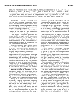
Figure 1: Histogram of Data Set I
60
50
40
30
20
10
0
0.2
0.4
0.6
0.8
1
1.2
1.4
1.6
1.8
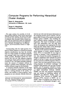
Figure 1: Histogram of Data Set I with 400 pts.
the centroid positions, are computed at various values of . These centroids cluster the input data
at a scale determined by .
We consider three problems of increasing complexity, namely, a simple one-dimensional data
set, the classic Iris data set and a high dimensional real breast cancer data set. A histogram of
Data set I is shown in Fig. 1. Even though, at a rst glance, this data set appears to have 4 clusters
it can be seen that at a larger scale only 2 clusters are present. The Iris data consists of labeled
data from 3 classes. The third data set contains 9-dimensional features characterizing breast cancer
and is collected from University of Wisconsin Hospitals, Madison, from Dr. William H. Wolberg.
It is also a part of the public-domain PROBEN1 benchmark suite [Pre94].
The procedure followed in performing the clustering at dierent scales is now briey described.
We start with a large number of RBF nodes and initialize the centroids by picking at random from
the data set on which clustering is to be performed. Then the following steps are executed:
Step 1: Start with a large number of \cluster representatives" or centroids. Each centroid is
represented by one hidden unit in the RBFN.
10
Step 2: Initialize these centroids by random selection from training data
Step 3: Initialize to a small value, o
Step 4: Iterate eqn.(6) on all centroids
Step 5: Eliminate duplicate centroids whenever there is merger
Step 6: Increase by a constant factor Step 7: If there are more than one unique centroid, go to Step 4
Step 8: Stop when only one unique centroid is found
At any desired scale, clustering is performed by assigning each data point to the nearest centroid,
determined using a suitable metric. In Step 5, a merger is said to occur between two centroids xc
and x0c , when kxc ? x0c k < , where is a small positive value which may vary with the problem.
The question of proper scale selection and the quality of resulting clusters is addressed in Section
4.
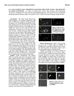
For simulation with Data Set I, 14 RBF nodes are used. The centroids are initialized by a
random selection from the input data set. As is increased neighboring centroids tend to merge at
certain values of . Change in location of centroids as is varied is depicted as a tree diagram in
Fig. 2. At = 0:05 only 4 branches can be seen i.e., there are only 4 unique centroids located at
0:51; 0:74; 1:43 and 1:66; the rest are copies of these. Every other branch of the initial 14 branches
merged into one of these 4 at some lower value of . Henceforth these branches do not vary much
over a large range of until at = 0:2 the 4 branches merge into 2 branches. When the \lifetimes"
of these branches are calculated, it is found that the earlier 4 branches have longer lifetime than
the later 2 branches.2 Hence these 4 clusters provide the most natural clustering for the data set.
2
The concept of lifetimes is introduced in Section 4.
11
Figure 2: Cluster Tree for Data Set I with Gaussian RBF
1.8
1.6
1.4
Centroids
1.2
1
0.8
0.6
0.4
0.2 −3
10
−2
−1
10
10
0
10
Scale
Figure 2: Cluster Tree for Data Set I with 14 RBF nodes. Only 13 branches seem to be present
even at the lowest scale because the topmost \branch" is actually two branches which merge at
= 0:002.
12
In general, two types of bifurcations occur in clustering trees such as the one in Fig. 2: (i) pitchfork and (ii) saddle-node bifurcations [Won93]. In the former type, two clusters merge smoothly
into one another, and in the latter, one cluster becomes unstable and merges with the other. Pitchfork bifurcation occurs when the data distribution is largely symmetric at a given scale; otherwise
a saddle-point bifurcation is indicated. Since the data set I is symmetric at a scale larger than 0:05,
pitchfork bifurcation is observed in Fig. 2. For smaller scales saddle-bifurcations can be seen.
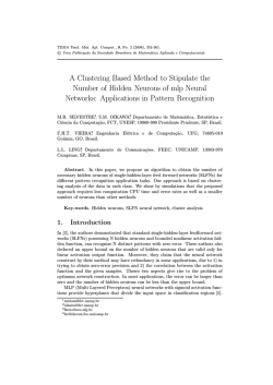
The Iris data is a well-known known benchmark for clustering and classication algorithms. It
contains measurements of 3 species of Iris, with 4 features (petal length, petal width, sepal length
and sepal width) in each pattern. The data set consists of 150 data points, all of which are used for
clustering and for subsequent training. The number of clusters produced by the RBFN at various
scales is shown in Fig. 3. It must be remembered that class information was not used to form the
clusters. At = 0:5, 4 clusters are obtained. These are located at,
(a)4:98; 3:36; 1:48; 0:24;
(b)5:77; 2:79; 4:21; 1:30;
(c)6:16; 2:86; 4:90; 1:70;
(d)6:55; 3:04; 5:44; 2:10:
It can be seen that centroids (b) and (c) are close to each other. Since the centroids have no
labels on them we gave them following class labels: (a) - Class I, (b) & (c) - Class II, and (d) Class III. The classication result with these 4 clusters is given in Table 1. In order to compare
the performance with other methods that use only 3 clusters for this problem we omitted one of
(b) and (c) and classied the iris data. Performance results with the cluster centers fa, b, dg and
fa, c, dg are given in Tables 2 and 3 respectively. It will be noted that the performance is superior
to the standard clustering algorithms like FORGY and CLUSTER which committed 16 mistakes
each [Jai86]. Kohonen's Learning Vector Quantization algorithm committed 17 mistakes on this
problem [PBT93].
Since the ideal clusters for Iris data are not spherical, it is possible to normalize or rescale the
13
Figure 3: Number of Clusters vs. Scale for Iris data
15
Number of Clusters
10
5
0 -2
10
-1
0
10
10
1
10
Scale
Figure 3: Number of clusters vs. scale for Iris Data
inputs to get better performance. In particular, one can rescale the individual components so that
their magnitudes are comparable (feature1 feature1 =3; feature3 feature3 =2). For this case,
at = 0:39 the network produced 3 clusters that yielded perfect classication for all the 150 patterns
in the data set (see Table 4). In Section 9, a technique for adaptively introducing anisotropicity
in the clustering process by allowing dierent widths in dierent dimensions, is suggested. Such a
facility can reap the fruits of rescaling without an explicit input preprocessing step.
The breast cancer data set has 9 attributes which take integral values lying in 1 ? 10 range.
Each instance belongs to one of two classes, benign or malignant. There are totally 683 data points,
all of which are used for clustering and also for testing. The network was initialized with 10 RBFs.
At = 1:67, 8 of the initial clusters merged into a single cluster, leaving 3 distinct clusters. As
class information was not used in the clustering process, classes must be assigned to these clusters.
We assumed that the cluster into which 8 clusters have merged to be of benign type since it is
known beforehand that a major portion (65:5%) of the data is of this type. The other two clusters
14
Table 1: Confusion Matrix for Iris data (4 clusters)
Cluster number
a
b, c
d
Class I
50
0
0
Class II Class III
0
0
50
15
0
35
Table 2: Confusion Matrix for Iris data (3 clusters: a,b and d)
Cluster number
a
b
d
Class I
50
0
0
Class II Class III
0
0
44
5
6
45
Table 3: Confusion Matrix for Iris data (3 clusters: a, c and d)
Cluster number
a
c
d
Class I
50
0
0
15
Class II Class III
2
0
48
15
0
35
Table 4: Confusion Matrix for Iris data (3 clusters with scaling)
Cluster number
1
2
3
Class I
50
0
0
Class II Class III
0
0
50
0
0
50
Table 5: Confusion Matrix for Breast Cancer Data
Predicted Class
Benign
Malignant
Actual Class
Benign Malignant
437
28
7
211
are assigned to the malignant category. With this cluster set a 1-nearest neighbor classier yielded
95:5% correct classication (see Table 5). In comparison, a study which applied several instancebased learning algorithms on a subset of this data set, reported best classication result of 93:7%
[Zha92] even after taking into account category information.
4 Cluster Validity
The issue of cluster validity is sometimes as important as the clustering task itself. It addresses
two questions: (1) How many clusters are present? (2) are the clusters obtained \good" [DJ79]?
A cluster is good if the distances between the points inside the cluster are small, and the distances
from points that lie outside the cluster are relatively large. The notion of compactness has been
proposed to quantify these properties [Jai86]. For a cluster C of n points, compactness is dened
16
as,
of each point in C which belong to C :
compactness = number of n ? 1 nearest neighbors
n(n ? 1)
A compactness value of 1 means that the cluster is extremely compact.
A related measure is \isolation" which describes how isolated a cluster is from the rest of the
points in the data. Variance-based measures such as the within-cluster and between-cluster scatter
matrices, also capture more or less the same intuitive idea [DH73].
From a scale-based perspective, we may argue that the idea of compactness, like the idea of
a cluster itself, is scale-dependent. Hence we will show that the concept of compactness can be
naturally extended to validate clusters obtained by a scale-based approach. The compactness
measure given above, then, can be reformulated as follows:
P 2C exp(?kx ? x k2=2)
compactnessi = P Pi
;
2
2C j exp(?kx ? x k = 2)
i
x
x
i
(12)
j
When clusters are obtained at a scale, , are \true" clusters, one may expect that most of the
points in a cluster, Ci , should lie within a sphere of radius, . The compactness dened in (12), is
simply a measure of the above property, a high value of which implies that points in Ci contribute
mostly to Ci itself. Thus, for a good cluster, compactness and isolation are close to 1. This new
measure is clearly computationally much less expensive than the earlier compactness. It is also less
cumbersome than the within-class and between-class scatter matrices.
It can be seen that compactness is close to 1 for very large or very small values of . This is
not a spurious result, but is a natural consequence of a scale-dependent cluster validation criterion.
It reects our earlier observation that at a very small scale every point is a cluster and at a large
enough scale the entire data set is a single cluster. The problem arises with real-world situations
because real data sets are discrete and nite in extent. This problem was anticipated in imaging
situations by Koenderink [Koe84], who observed that any real-world image has two limiting scales;
17
the outer scale corresponding to the nite size of the image, and an inner scale given by the
resolution of the imaging device or media.
In hierarchical schemes, a valid cluster is selected based on its lifetime and birthtime. Lifetime
is dened as the range of scale between the point when the cluster is formed and the point when
the cluster is merged with another cluster. Birth time is the point on the tree when the cluster is
created. An early birth and a long life are characteristics of a good cluster. In the tree diagram
for Data Set I (Fig. 2), it can be veried that the 4 branches that exist over 0:05 < < 0:2 satisfy
these criteria. From Fig. 4 the cluster set with longest lifetime, hence indicating the right scale,
can be easily determined. Here it must be remembered that the tree is biased on the lower end of
, because we start from a lower scale with a xed number of centroids and move upwards on scale.
If we proceed in the reverse direction, new centroids may be created indenitely as we approach
lower and lower scales. Therefore we measure lifetimes only after the rst instance of merger of a
pair (or more) of clusters.
In the above method we selected as a good partition the one that has the longest lifetime. Here
we introduce an alternative method that denes a cost functional which takes low values for a good
partition. This cost depends on the compactness of clusters as dened in (12). A good partition
should result in compact clusters. For a partition with n clusters, the above cost can be dened as,
overall compactness cost = (n ?
Xn compactness )2;
i
i
(13)
where compactnessi is the compactness of the ith cluster. Since compactness for a good cluster
is close to 1 the above cost is a small number for a good partition.
The above technique is tested on a 10-dimensional data set with 8 clusters. The cluster centers
are located at 8 well-separated corners of a 10-dimensional hypercube. All the points in a cluster
lie inside a ball of radius 0:6 centered at the corresponding corner. Fig. 5 shows a plot of the
compactness cost vs. the number of clusters at a given . The cost dropped to 0 abruptly when
the number of clusters dropped to 8 and remained so over a considerable span of .
18
Figure 4: Number of clusters vs. scale for Data Set I
10
9
8
Number of clusters
7
6
5
4
3
2
1 -3
10
-2
-1
10
10
Scale
0
1
10
10
Figure 4: Number of clusters vs. scale for Data Set I
Figure 5: Compactness Cost for 10-D data with 8 clusters
150
Compactness Cost
100
50
0
0
2
4
6
8
10
12
Number of clusters
14
16
18
20
Figure 5: Compactness cost for the 10-dimensional data set with 8 clusters (see text for data
description). Compactness cost is zero at and around 8 clusters
19
In the framework of our scale-based scheme, compactness measure seems to be a promising
tool to nd good clusters or the right scale. It has the desirable property that the approach used
for forming clusters and the rule for picking good clusters are not the same. The ecacy of the
procedure in higher dimensions must be further investigated.
5 Computation Cost and Scale
The computation required to nd the correct centroids for a given data set depends on (i) how
many iterations of eqn.(6) are needed at a given , and (ii) how many dierent values of need
to be examined. The number of iterations needed for eqn.(6) to converge depends on the scale
value in an interesting way. We have seen that a signicant movement of centroids occurs in the
neighborhood of bifurcation points, while between any two adjacent bifurcation points there is
usually little change in centroid locations. In this region, if the centroids are initialized by the
centroid values obtained at the previous scale value, convergence occurs within a few (typically
two) iterations.
The number of iterations required to converge are plotted against the scale value in Fig. 6b for
the articial data set I. The corresponding cluster tree is given in Fig. 6a for direct comparison.
The discrete values of scale at which centroids are computed are denoted by `o's in Fig. 6b. The
step-size, , a factor by which scale is multiplied at each step, is chosen to be 1:05. It can be
seen that major computation occurs in the vicinity of the bifurcation points. However a curious
anomaly occurs in Fig. 6b near = 0:2 and 0:8, where there is a decrease in number of iterations.
A plausible explanation can be given. Number of iterations required for convergence at any depends on how far the new centroid, denoted by xj (n+1 ), is from the previous centroid, xj (n ).
Hence, computation is likely to be high when the derivative of the function xj ( ) w.r.t is high
or discontinuous in the neighborhood of . In Fig. 6b, at = 0:2 and 0:8, it can be seen that
centroids merge smoothly, whereas, at other bifurcation points, one of the branches remains at
20
while the other bends and merges in it at an angle.
A similar plot for a slightly larger stepsize (= 1:15) in scale is shown in Fig. 7b with corresponding cluster tree in Fig. 7a. One may expect that, since the scale values are now further apart,
there will be an overall increase in the number of iterations required to converge. But Fig. 7b
shows that there is no appreciable change in overall computation compared to the previous case.
Computation is substantial only close to the bifurcation points, except near the one at = 0:8,
presumably for reasons of smoothness as in the previous case.
Therefore, for practical purposes one may start with a reasonably large stepsize, and if more
detail is required in the cluster tree, a smaller step size can be temporarily used. Simulations
with other data sets also demonstrate that no special numerical techniques are needed to track
bifurcation points, and a straightforward exploration of the scale-space at a fairly large step-size
does not incur any signicant additional computation.
6 Coupling among Centroid Dynamics
In eqn.(5) one may note that the weight, w, introduces a coupling between the dynamics of individual centroids. The term w appears at two places in eqn.(5): in the learning rate, 4(= 2w),
P
and in the error term, (1 ? j wRj (x)). We need not concern ourselves with w in 4 because 2
can be arbitrarily chosen to obtain any value of 4. But w has a signicant eect on the error term.
When w ! 0, the centroids move independent of each other, whereas for a signicant value of w
the dynamics of individual centroids are tightly coupled and the approximation that yields eqn.
(6) is no longer valid. Hence, for a large value of w, it is not clear if one may expect a systematic
cluster merging as the scale is increased. We found that the w can be considered as a \coupling
strength", which can be used to control the cluster tree formation in a predictable manner.
Recall that the cluster tree for data set I shown in Fig. 2 is obtained using eqn. (6) i.e. for
w ! 0. But when w is increased to 0:86 the two nal clusters fail to merge (Fig. 8). As w is further
21
Figure 6a: Cluster Tree for Data Set I
Centroids
2
1
0 −3
10
−2
−1
10
10
0
10
Scale
Figure 6b: Computation Cost for the above plot
Number of Iterations
60
40
20
0 −3
10
−2
−1
10
10
Scale
Figure 6: Computation cost for Data Set I at a step-size of 1:05.
22
0
10
Figure 7a: Cluster Tree for Data Set I
Centroids
2
1
0 −3
10
−2
−1
10
0
10
10
Scale
Figure 7b: Computation Cost for the above plot
1
10
Number of Iterations
60
40
20
0 −3
10
−2
10
−1
10
Scale
0
10
Figure 7: Computation cost for Data Set I at a step-size of 1:15.
23
1
10
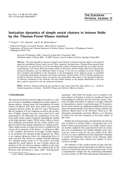
Figure 8: Effect of centroid coupling (w = 1.2/N) on the cluster tree
1.8
1.6
1.4
Centroids
1.2
1
0.8
0.6
0.4
0.2 −3
10
−2
−1
10
10
Scale
0
10
1
10
Figure 8: Eect of large w(= 1:2=N ) on the cluster tree for Data Set I. Eqn. (6) is used for
clustering and data is presented in batch mode. Tree develops normally up to a scale beyond which
clusters fail to merge.
increased cluster merger fails to occur even at much lower scales. The question that now arises
is: why and for what range of w does \normal" merger of clusters occur? A simple calculation
P
yields an upper bound for w. The error term, (1 ? j wRj (x)), in eqn.(5) must be positive for the
clustering process to converge. For large , Rj (x) ! 1 so that,
N
X
wR (x) Nw;
j
j
where N is the number of RBF nodes. The error term is positive if Nw < 1, or, w < 1=N . From
simulations with a variety of data sets and a range of network sizes we found that a value of w that
is slightly lesser than 1=N does indeed achieve satisfactory results.
A non-zero w also plays a stabilizing role on cluster tree formation. The cluster tree in Fig. 2
is obtained, in fact, by simulating eqn. (6) (i.e. (5) with w = 0) in batch mode. But when (5) is
simulated with w = 0, (same as eqn. (6)) using on-line mode with synchronous data presentation
24
Figure 9: Effect of small w (= 0.0) on the cluster tree
1.8
1.6
1.4
Centroids
1.2
1
0.8
0.6
0.4
0.2 -3
10
-2
10
-1
10
Scale
0
10
1
10
Figure 9: Eect of small w(= 0:0) on the cluster tree for Data Set I, when data is presented online in synchronous mode. Tree is biased towards one of the component clusters at the points of
merging.
(i.e. inputs are presented in the same sequence in every epoch), the cluster tree obtained is biased
towards one of the component clusters at the point of merging. For instance, in Fig. 9, a saddlenode bifurcation occurs at = 0:106, in spite of the symmetric nature of the data at that scale. But
a symmetric tree is obtained even with synchronous updating by using eqn. (5) with w = 0:07 (Fig.
10). In Fig. 9, biasing of tree occurred not because w = 0, but due to synchronous updating, since
a symmetric tree is obtained with w = 0 in batch mode. Hence, a non-zero value of w seems to have
a stabilizing eect (in Fig. 10) by which it osets the bias introduced by synchronous updating (in
Fig. 9). The above phenomenon points to a certain instability in the dynamics of eqn. (6) which
is brought forth by synchronous input presentation. An in-depth mathematical study conrms this
observation and explains how a non-zero w has a stabilizing eect. However, the study involves
powerful tools of catastrophe or singularity theory [Gil81], [Lu76], which is beyond the scope of the
present paper. The details of this work will be presented in a forthcoming publication.
25
Figure 10: Effect of non-zero w ( = 0.07) on cluster tree for Data Set I
1.8
1.6
1.4
Centroids
1.2
1
0.8
0.6
0.4
0.2 -3
10
-2
10
-1
0
10
Scale
10
1
10
Figure 10: Eect of non-zero w(= 0:07) on the cluster tree for Data Set I, when data is presented
on-line in synchronous mode. A symmetric tree is obtained.
7 Clustering Using Other Basis Functions
Qualitatively similar results of scale-based clustering are also obtainable by several other (nongaussian) RBFs provided such basis functions are smooth, \bell-shaped", non-negative and localized. For example, the cluster tree for Data Set I obtained using the RBF dened as,
R(x) = 1 + kx ?1 x k2 =2
j
is shown in Fig. 11. It is remarkable that the prominent clusters are nearly the same as those
obtained with a gaussian nonlinearity (see Fig. 2). A similar tree is obtained using, R(x) =
1
1+k ? k = . One the other hand, with functions that take on negative values such as the sinc()
and the DOG(), merging of clusters does not always occur and sometimes there is cluster splitting
as is increased (see Figs. 12 & 13).
All of the functions considered above are radially symmetric, smooth etc. Yet progressive merger
x
xj 4
4
26
Figure 11: Cluster tree for Data Set I with inverse quadratic RBF
1.8
1.6
1.4
Centroids
1.2
1
0.8
0.6
0.4
0.2 -3
10
-2
10
-1
10
Scale
0
10
1
10
Figure 11: Cluster tree for Data Set I with inverse quadratic RBF
Figure 12: Cluster tree for Data Set I with Sinc(.) RBF
4
3
Centroids
2
1
0
-1
-2 -3
10
-2
10
-1
10
Scale
0
10
1
10
Figure 12: Cluster tree for Data Set I with Sinc() RBF
27
Figure 13: Cluster tree for Data Set I with DOG(.) RBF
8
6
Centroids
4
2
0
-2
-4
-6 -3
10
-2
10
-1
0
10
Scale
1
10
10
Figure 13: Cluster tree for Data Set I with dierence of gaussian RBF
of clusters did not take place with some functions. Why is this so? It appears that there must be
special criteria which a function suitable for scale-based clustering must satisfy. These questions
have already been raised by scale-space theory [Lin90], [Lin94], and answered to a large extent using
the notion of scale-space kernels. A good scale-space kernel should not introduce new extrema on
convolution with an input signal. More formally, a kernel h 2 L1 is a scale-space kernel if for any
input signal f 2 L1 , the number of extrema in the convolved signal f = h f is always less than or
equal to the number of local extrema in the original signal. In fact, such kernels have been studied
in classical theory of convolutions integrals [HW55]. It is shown that a continuous kernel h is a
scale-space kernel if and only if it has a bilateral Laplace-Steltjes transform of the form,
Z1
x=?1
eais
h(x)e?sx dx = Cecs +bs 1
i=1 1 + a s
2
i
P
2
where, (?d < Re(s) < d), for some d > 0, C 6= 0, c 0, b and ai are real, and 1
i=1 ai is
convergent. These kernels are also known to be positive and unimodal both in spatial and in the
28
frequency domain.
The gaussian is obviously unimodal and positive both in spatial and frequency domains. The
inverse quadratic function, 1+kx1k = , is clearly positive and unimodal in spatial domain, and it is
so in transform domain also since its frequency spectrum is of the form e?kf k , where > 0. On
the other hand, these conditions are obviously not satised by the sinc() and DOG() functions
since they are neither positive nor unimodal even in the spatial domain.
2
2
8 RBFN as a Multi-scale Content-Addressable Memory
Dynamic systems in which a Lyapunov function describes trajectories that approach basins of
attraction have been used as Content Addressable Memories (CAMs) [Hop84]. The idea of a
Multi-scale CAM (MCAM) is best expressed using a simple example. The simple one-dimensional
data set shown in Fig. 1 can be used to for this purpose. When clustered at = 0:07, the data set
reveals 4 clusters, A1 ; A2; B1 and B2 , centered at 0:51; 0:74; 1:43 and 1:66, respectively. At a slightly
larger scale, i.e., = 0:3, only 2 clusters (A = fA1 A2 g and B = fB1 B2 g) are found, centered at
0:65 and 1:55 respectively (see Fig. 2). An MCAM in which the above data is stored is expected
to assign a novel pattern to one of the specic clusters, i.e., Ai or Bi , or more generally to A or B ,
depending on the resolution determined by the scale parameter, .
The MCAM operates in distinct (1) storing and, (2) retrieval phase.
Storing:
(i) The network is trained using eqn.(6) on data in which clusters are present at several scales.
Training is done at the smallest scale, min , at which MCAM will be used, and therefore a large
number of hidden nodes are required.
(ii) The set of unique clusters, x , obtained constitutes the memory content of the network.
Retrieval:
(i) Construct a RBFN with a single hidden node whose centroid is initialized by the incomplete
j
29
pattern, x, presented to the MCAM.
(ii) Fix the width at a value of scale at which search will be performed.
(iii) Train the network with the cluster set x as the training data using eqn. (6). The centroid of
the single RBF node obtained after training is the retrieved pattern.
The data set I can be used again to illustrate the MCAM operation. In the storing stage the
data set consisting of 400 points is clustered at a very small scale (min = 0:0012). Clustering
yielded 22 centroids which form the memory content of the MCAM. In the retrieval stage, the
network has a single RBF node whose centroid is initialized with the corrupt pattern, xinit = 0:68.
Eqn.(6) is now simulated at a given scale, as the the network is presented with the centroid set
obtained in the storing stage. The retrieved pattern depends both on the initial pattern and also
on the scale at which retrieval occurs. For 0:08, the center of the subcluster A2 is retrieved
(xfinal = 0:74) and for 2 (0:2; 0:38), the larger cluster A (=fA1, A2g) is selected (xfinal = 0:65).
j
9 Discussion
By xing the weights from the hidden units to the output, and having a \dummy" desired target,
the architecture of RBFN is used in a novel way to accomplish clustering tasks which a supervised feedforward network is not designed to do. No apriori information is needed regarding the
number of clusters present in the data, as this is directly determined by the scale or the width
parameter, which acquires a new signicance in our work. This parameter has not come to be
treated in the same manner by RBFN studies in the past for several reasons. In some of the early
work which popularized RBFNs, the label \localized receptive elds" has been attached to these
networks [MD89]. Width is only allowed to be of the same scale as that of the distance between
centroids of neighboring receptive elds. But this value depends on the number of centroids chosen. Therefore, usually the question of right number of centroids is taken up rst, for which there
is no satisfactory solution. Since the choice of the number of centroids and the width value are
30
interrelated, we turn the question around and seek to determine the width(s) rst by a scale-space
analysis. Now the interesting point is, the tools required for the scale space analysis need not be
imported from elsewhere, but are inherent in the gradient descent dynamics of centroid training.
Once the right scale or scale interval is found, the number of centroids and the width value are
automatically determined. The benet of doing this is twofold. On one hand, we can use the RBF
network for scale-based clustering which is an unsupervised procedure, and on the other we have
a systematic way of good initialization for the RBF centers and width, before proceeding with the
usual supervised RBFN training.
From eqn. (8), one can show that,
P xRj (x)
x = P R (x) :
j
j
x
x
(14)
Note that in eqn. (14) x is covertly present in the R.H.S. also, which can be solved for iteratively
by the following map:
P
x (t + 1) = P xRRj((xx)) :
(15)
j
x
j
x
j
This form is reminescent of the iterative rule that determines means of the component distributions,
when the Expectation Maximization (EM) [RW84] algorithm is used to model a probability density
function. Recently, the EM formulation has been used to compute hidden layer parameters of the
RBF network [UH91]. The dierence is that, in the EM approach, number of components need to
be determined apriori, and the priors (weights) as well as widths of components are also adapted.
Our approach essentially gives the same weight to each component, and determines number of
components for a given width (scale) which is the same for all the components.
Our scheme partitions data by clustering at a single scale. This may not be appropriate if
clusters of dierent scales are present in dierent regions of the input space. If one may draw an
analogy with the Gaussian mixture model, this means that the data has clusters with dierent
variances. Our present model can easily be extended to handle such a situation if we use a dierent
width for each RBF node, and then multiply these widths by a single scale factor. The widths
31
are given as, j = dj , where is the new scale parameter and dj is determined adaptively by
modifying (4) as,
2
dj = 3Rj (x ) kx ?4dx3 k :
(16)
p
j
p
j
Note that w is still a small constant and therefore the (1 ? f (x )) term can be neglected. Now, for
every value of both the cluster centers, x , and the RBF widths j are determined using (6) and
(16).
Another limitation of our model might arise due to the radially symmetric nature of the RBF
nodes. This may not be suitable for data which are distributed dierently in dierent dimensions.
For these situations, RBFs can be replaced by Elliptic Basis Functions (EBFs)
p
j
Ej (xp) = e
? 12 k (xpk?2xjk )
jk
2
:
(17)
which have a dierent width in each dimension. The network parameters of EBF are computed
by gradient descent. The weight update equation is the same as (2), but the centroid and width
updates are slightly dierent:
X
x = E (x ) (xpk ? xjk ) ( (tp ? f (x ))w );
(18)
jk
2 j
p
jk2
i
i
i
p
ij
2 X
jk = 3Ej (x ) (xpk ?3 xjk ) ( (tpi ? fi (x ))wij ):
p
jk
i
p
(19)
EBF networks often perform better on highly correlated data sets, but involve adjustment of extra
parameters [BG92].
Even though the present work is entirely devoted to evaluating RBFN as a clustering machine,
more importantly it remains to be seen how the method can be used for RBFN training itself.
For training RBFN then, the network is rst put in unsupervised mode, and scale-based clustering
is used to nd centroids and widths. Subsequently, the second stage weights can be computed
adaptively using (2) or by a suitable pseudoinversion procedure. A task for the future is to assess
the ecacy of such a training scheme.
32
The RBFN has several desirable features which renders work with this model interesting. In
contrast to the popular Multi-Layered Perceptron (MLP) trained by backpropagation, RBFN is
not \perceptually opaque". For this reason training one layer at a time is possible without having
to directly deal with an all-containing cost function as in the case of backpropagation. In another
study, the present authors describe how Self-Organized Feature Maps can be constructed using
RBFN, for 1-D data [GC94]. The same study analytically proves that the map generated by RBFN
is identical to that obtained by Kohonen's procedure in the continuum limit. Work is underway to
extend this technique for generating maps of higher dimensions. Relating RBFN to other prominent
neural network architectures has obvious theoretical and practical interest. Unifying underlying
features of various models brought out by the above-mentioned studies, is of theoretical importance.
On the practical side, incorporating several models in a single architecture is benecial for eective
and ecient VLSI implementation.
33
References
[BA83]
P.J. Burt and E.H. Adelson. The Laplacian pyramid as a compact image code. IEEE
Trans. Communications, 9:4:532{540, 1983.
[BG92]
S. Beck and J. Ghosh. Noise sensitivity of static neural classiers. In SPIE Conf. on
Science of Articial Neural Networks SPIE Proc. Vol. 1709, Orlando, Fl., April 1992.
[BL88]
D.S. Broomhead and D. Lowe. Multivariable functional interpolation and adaptive
networks. Complex Systems, 2:321{355, 1988.
[DH73]
R. O. Duda and P. E. Hart. Pattern Classication and Scene Analysis. Wiley, New
York, 1973.
[DJ79]
R. Dubes and A. K. Jain. Validity studies in clustering methodologies. Pattern Recognition, 11:235{254, 1979.
[Eve74]
B. Everitt. Cluster Analysis. Wiley, New York, 1974.
[FRKV92] L.M.J. Florack, B.M. ter Haar. Romney, J.J. Koenderink, and M.A. Viergever. Scale
and the dierential structure of images. Image and Vision Computing, 10:376{388, July
1992.
[GBD92] J. Ghosh, S. Beck, and L. Deuser. A neural network based hybrid system for detection,
characterization and classication of short-duration oceanic signals. IEEE Jl. of Ocean
Engineering, 17(4):351{363, October 1992.
[GC94]
J. Ghosh and S. V. Chakravarthy. Rapid kernel classier: A link between the selforganizing feature map and the radial basis function network. Journal of Intelligent
Material Systems and Structures, 5:211{219, March 1994.
34
[Gil81]
R. Gilmore. Catastrophe Theory for Scientists and Engineers. Wiley-Interscience, New
York, 1981.
[Hop84]
J. J. Hopeld. Neurons with graded response have collective computational properties
like those of two-state neurons. Proc. National Academy of Sciences, USA, 81:3088{
3092, May 1984.
[HW55]
I.I. Hirschmann and D.V. Widder. The convolution transform. Princeton University
Press, Princeton, New Jersey, 1955.
[Jai86]
A. K. Jain. Cluster analysis. In T.J. Young and K. Fu, editors, Handbook of Pattern
Recognition and Image Processing, pages 33{57. Academic Press, 1986.
[KGV83] S. Kirkpatrick, C. D. Jr Gelatt, and M. P. Vecchi. Optimization by simulated annealing.
Science, 220:671{680, May 1983.
[Kit76]
J. Kittler. A locally sensitive method for cluster analysis. Pattern Recognition, 8:23{33,
1976.
[Kli71]
A. Klinger. Pattern and search statistics. In J.S. Rustagi, editor, Optimizing methods
in ststistics. Academic Press, New York, 1971.
[Koe84]
J.J. Koenderink. The structure of images. Biol. Cyber., 50:363{370, 1984.
[Lin90]
T. Lindeberg. Scale-space for discrete signals. IEEE Trans. Patt. Anal. and Mach.
Intell., 12:234{254, 1990.
[Lin94]
T. Lindeberg. Scale-space theory in computer vision. Kluwer Intl. Series in Eng. and
Comp. Sci., Kluwer Academic Publishers, 1994.
[LJ89]
Y. Lu and R.C. Jain. Behavior of edges in scale space. IEEE Trans. PAMI, 11:4:337{356,
1989.
35
[Lu76]
Y.C. Lu. Singularity Theory and an introduction to catastrophe theory. Springer-Verlag,
New York, 1976.
[LW91]
D. Lowe and A. R. Webb. Optimized feature extraction and the bayes decision in
feed-forward classier networks. IEEE Trans. PAMI, 13:355{364, April 1991.
[Mal89]
S.G. Mallat. A theory for multi-resolution signal decomposition: The wavelet representation. IEEE Trans. Patt. Anal. and Mach. Intell., 11:7:674{694, 1989.
[MB88]
G.J. McLachlan and K.E. Basford. Mixture Models: Inference and applications to clustering. Dekker, New York, 1988.
[MD89]
J. Moody and C. J. Darken. Fast learning in networks of locally-tuned processing units.
Neural Computation, 1(2):281{294, 1989.
[Par62]
E. Parzen. On estimation of a probability density function and mode. Annals of Mathematical Statistics, 33:1065{1076, 1962.
[PBT93] N. R. Pal, J. C. Bezdek, and E. C.-K. Tsao. Generalized clustering networks and
Kohonen's self-organizing scheme. IEEE Transactions on Neural Networks, 4:549{557,
July 1993.
[PG90]
T. Poggio and F. Girosi. Networks for approximation and learning. Proc. IEEE,
78(9):1481{97, Sept 1990.
[Pow85]
M.J.D. Powell. Radial basis functions for multivariable interpolation: A review. In
Proc. of IMA Conference on Algorithms for Approximation of Functions and Data,
pages 143{167, RMCS, Shrivenham, UK, 1985.
[Pre94]
L. Prechelt. Proben1 - a set of neural network benchmark problems and benchmarking rules. Technical Report 21/94, Universitat Karlsruhe, 76128 Karlsruhe, Germany,
September 1994.
36
[RGF90] K. Rose, E. Gurewitz, and G. C. Fox. A deterministic annealing approach to clustering.
Pattern Recognition Letters, 11:589{594, September 1990.
[RW84]
R. A. Redner and H. F. Walker. Mixture densities, maximum likelihood and the EM
algorithm. SIAM Review, 26:195{239, April 1984.
[TGK90] P. Tavan, H. Grubmuller, and H. Kuhnel. Self-organization of associative memory
and classication: Recurrent signal processing on topological feature maps. Biological
Cybernetics, 64:95{105, 1990.
[UH91]
A. Ukrainec and S. Haykin. Signal processing with radial basis function networks using
expectation maximization algorithm clustering. In Proc. of SPIE, Vol. 1565, Adaptive
Signal Processing, pages 529{539, 1991.
[Wit83]
A. P. Witkin. Scale-space ltering. In Proc. 8th Int. Joint Conf. Art. Intell. (Karlsruhe,
Germany), pages 1019{1022, August 1983.
[Won93] Y. F. Wong. Clustering data by melting. Neural Computation, 5(1):89{104, 1993.
[Zha92]
J. Zhang. Selecting typical instances in instance-based learning. In Proc. of the Ninth
International Machine Learning Conference, pages 470{479, 1992.
37