1. Art and Diseño

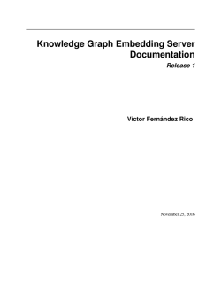
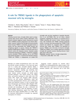
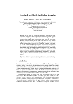
TEMA Tend. Mat. Apl. Comput., 9, No. 2 (2008), 351-361.
c Uma Publica¸c˜
ao da Sociedade Brasileira de Matem´
atica Aplicada e Computacional.
A Clustering Based Method to Stipulate the
Number of Hidden Neurons of mlp Neural
Networks: Applications in Pattern Recognition
M.R. SILVESTRE1, S.M. OIKAWA2, Departamento de Matem´
atica, Estat´ıstica e
Ciˆencia da Computa¸ca˜o, FCT, UNESP, 19060-900 Presidente Prudente, SP, Brasil.
F.H.T. VIEIRA3, Engenharia El´etrica e de Computa¸ca˜o, UFG, 74605-010
Goiˆ
ania, GO, Brasil.
L.L. LING4, Departamento de Comunica¸co˜es, FEEC, UNICAMP, 13083-970
Campinas, SP, Brasil.
Abstract. In this paper, we propose an algorithm to obtain the number of
necessary hidden neurons of single-hidden-layer feed forward networks (SLFNs) for
different pattern recognition application tasks. Our approach is based on clustering analysis of the data in each class. We show by simulations that the proposed
approach requires less computation CPU time and error rates as well as a smaller
number of neurons than other methods.
Key-words. Hidden neurons, SLFN neural network, cluster analysis.
1.
Introduction
In [3], the authors demonstrated that standard single-hidden-layer feedforward networks (SLFNs) possessing N hidden neurons and bounded nonlinear activation hidden function, can recognize N distinct patterns with zero error. These authors also
deduced an upper bound on the number of hidden neurons that are valid only for
linear activation output function. Moreover, they claim that the neural network
construct by their method may have redundancy in some applications, due to 1) in
trying to obtain zero-error precision and 2) the correlation between the activation
function and the given samples. Theses two aspects give rise to the problem of
optimum network construction. In most applications, the error can be larger than
zero and the number of hidden neurons can be less than the upper bound.
MLP (Multi Layered Perceptron) neural networks with sigmoid activation functions provide hyperplanes that divide the input space in classification regions [5].
1 [email protected]
2 [email protected]
3 [email protected]
4 [email protected]
352
Silvestre, Oikawa, Vieira and Ling
Therefore, one can construct hyperplanes by using the weights of the network. We
present an example of such a construction considering the XOR problem in Section
2.1.
Clustering techniques allow us to aggregate patterns that are close in space,
based on distance metrics. In this sense, clusters are used to divide the input
patterns in similar groups that can occupy different positions in the input space.
If there are two different neighbor clusters, it is possible to imagine that there
is a hyperplane that can separate these clusters. Then, if the number of cluster of
a dataset is known, we can assume that the same number (or less) of hyperplanes
are dividing them.
The initialization of neural networks through clustering techniques is the main
subject of many researches [2] and [9]. In [2], it is proposed an algorithm to initialize and optimize the MLP neural networks that does a particularly different
pre-processing in all input data and after that uses cluster analysis in step 2 and 3
to define weights of the hidden layer. Further, they propose an optimization of the
neural network based on penalty term. In the article [9], the authors suggest the
use of clustering and optimization techniques to select the hidden units of the initial
neural network configuration, but their method need to optimize a lot of different
sizes of network.
In this work, we propose an algorithm to define an appropriate number of hidden neurons of a MLP neural network, based on clustering methods. Our method
is simple than [2], because the variables are transformed to have zero mean and
one variance, and we used the standard backpropagation algorithm, without optimization of penalty parameters such as used by [2]. Also, we do not use clusters
optimization to select the size of the network as suggested by [9]. We investigated
the results obtained by our method using N hidden neurons sigmoid activation functions to output layer, instead of the linear activation output function proposed in
[3], because they are more appropriated to pattern recognition and classification
problems.
The rest of this paper is organized as follows. In Section 2, we recall some basic
theory involving neural networks and clustering techniques. In Section 3 we present
a description of the proposed cluster analysis method. In Section 4, we evaluate
the efficiency of the proposed algorithm by simulations and we discuss the obtained
results. Finally, in Section 5, we conclude.
2.
MLP Neural Network and Cluster Analysis
In this section, first of all we present some definitions related to the MLP neural
network in Section 2.1. Next, in Section 2.2, we give a general overview of cluster
analysis.
2.1.
MLP Network
Consider a MLP network, with one hidden layer (SLFN). Let [x(n), t(n)] denote
T
the nth (n = 1, ..., N ) training pattern where x(n) = [x1 (n), ..., xd (n)] is the d-
353
A Method to Stipulate the Number of Hidden Neurons
T
dimensional input feature vector and t(n) =n[t1 (n), ...,
toothe
o tc (n)] corresponds
n
(2)
(1)
(2)
(1)
desired c-class output response. Let W = wji (n) and W = wkj (n) be
the matrix of synaptic weights which connect the input to hidden layers and the
hidden to the output layers, respectively. The optimization procedure for classification consists of minimizing the sum of the mean square errors between the network
output yk (n) and the desired output tk (n), i.e.:
E=
N
P
E(n), where E(n) =
n=1
Assuming that g
(equation (2.1)):
(1)
and g
(2)
1
2
c
P
2
[yk (n) − tk (n)] .
k=1
are activation functions of sigmoid logistic type
g (.) (vj (n)) =
1
,
1 + exp (−pvj (n))
the k th network output yk (n) is given by yk (n) = g (2)
M
P
j=0
(2)
(2.1)
!
wkj (n)g (1) (vj (n)) ,
where M is the number of hidden neurons. If the equation (2.1) is applied to the
d
P
(1)
wji (n)xi (n); but if it is applied to the output layer,
hidden layer, then vj (n) =
d i=0
M
P
P (1)
(2)
(1)
wkj (n)g
vj (n) =
wji (n)xi (n) . Notice that the number of hidden neuj=0
i=0
rons in the hidden layer defines the maximum number of hyperplanes that delimit
decision boundaries in input feature space.
To exemplify how the delimit decision boundaries are created by the hidden
neurons, we will consider the XOR problem (Exclusive OR) with N = 4 patterns,
p = 2 variables (x1 and x2 ) and c = 2 classes (0 and 1). The input patterns are:
(0, 0) and (1, 1) that produces the class 0; and (0, 1), (1, 0) belong to class 1.
The training of a SLFN with M = 4 hidden neurons produces the W(1) matrix.
To each row (neuron) j = 1, ..., 4 of W(1) matrix, it is possible to construct a
hyperplane by varying the x1 and x2 variables according to the equation:
(1)
(1)
(1)
wj1 x1 + wj2 x2 + wj0 (−1) = 0.
The resulting M = 4 hyperplanes are presented in Figure 1 (graphic on the left),
and a more careful analysis of this Figure reveals that there are redundancies, e. g.
the problem need less than M = 4 hyperplanes to discriminate the two classes.
A SLFN with M = 2 hidden neurons can solve the XOR problem. The resulting
M = 2 hyperplanes are presented in Figure 1 (graphic on the right). It is clear that
the hyperplanes built with the weights of the hidden layer are able to divide the
input feature space in regions.
2.2.
Cluster analysis
In this section, we will focus on the clusters analysis. Traditional hierarchical clustering algorithms can be applied in classification tasks of many types of datasets.
The main purpose in cluster analysis is to aggregate similar patterns in groups.
354
1.5
1.5
1
1
x2
x2
Silvestre, Oikawa, Vieira and Ling
0.5
0
0.5
0
−0.5
−1.5
−1
−0.5
0
x1
0.5
1
1.5
−0.5
−1.5
−1
−0.5
0
x1
0.5
1
1.5
Figure 1: The XOR problem resolved with M = 4 hyperplanes (graphic on the left); and
with M = 2 hyperplanes (graphic on the right).
Firstly, it is necessary to define which measure of similarity or dissimilarity is
more appropriate for the clustering procedure. This measure is called ‘resemblance
coefficient’ and it is computed to each pair of patterns. An example of resemblance
coefficient is the Euclidean distance (equation (2.2)):
dab =
p
(x1 − y1 )2 + (x2 − y2 )2 +...+(xd − yd )2 .
(2.2)
There are others distance measures as Mean Euclidean distance, City-Block or
Manhattan distance, Minkowsky distance, coefficients of Gower, Catell, Camberra,
Bray-Curtis, Sokal-Sneath, Cosine, Pearson Correlation and many others.
Second, which method of clustering is to be used, the hierarchical clustering
techniques proceed by either a series of successive mergers, called Agglomerative
hierarchical methods, or a series of successive divisions, called Divisive hierarchical
methods. Agglomerative hierarchical methods start with the individual objects.
These methods initiate the algorithm with all patterns and they are aggregated
until the last one.
In this work, we pay attention on some methods classified as Agglomerative
hierarchical methods such as: Single Linkage, Complete Linkage, Average Linkage,
Median Linkage, Centroid, Ward and others.
In [4], the authors present an Agglomerative hierarchical method for clustering
N objects (in our case these objects are the patterns):
1.
Start with N clusters, each containing a single entity and an N × N
symmetric matrix of distances (or similarities) D = {dab } .
2.
Search the distance matrix for the nearest (most similar) pair of clusters.
Let the distance between “most similar” clusters U and V be dUV .
A Method to Stipulate the Number of Hidden Neurons
355
3.
Merge clusters U and V . Label the newly formed cluster (U V ). Update
the entries in the distance matrix by (a) deleting the rows and columns corresponding to clusters U and V and (b) adding a row and column giving the distances
between cluster (U V ) and the remaining clusters.
4.
Repeat Steps 2 and 3 a total of N − 1 times. (All objects will be in a
single cluster after the algorithm terminates). Record the identity of clusters that
are merged and the levels (distances or similarities) at which the mergers take place.
Now, we will describe some aspects and procedures belonging to the Agglomerative clustering methods. Initially one has to find the smallest distance in D = {dab }
and merge the corresponding patterns, say, U and V , to get the cluster (U V ). For
Step 3 of the general algorithm the distances between (U V ) and any other cluster W are computed by different ways in each clustering method: Single Linkage,
Complete Linkage, Average Linkage, Ward, Median Linkage and Centroid (more
details can be seen in [4]). Then, after the clustering method be applied there was
construct a new distance symetric matrix Dc = {dab }.
After the application of one or more methods mentioned above, it is necessary
to define how many clusters there are on the data, because the Agglomerative
algorithm aggregate all the patterns until just one cluster. Then it is necessary to
found a cut point on the dendrogram or tree graphic. The dendrogram is built with
the measure of distance in each pass of the clustering.
To define how is the better point to cut the tree you have to find a point where
the clustering of one pass to the next pass provided a large increase in the distance
or a jump. This means that were jointed two patterns/clusters that do not have
much in common, so a large distance measure was produced between them. So,
it is convenient decide to the number of clusters provided by the pass anterior to
the jump. The jump can be easily seen if we construct a graph with the distance
levels in each step of the linkage method. In this case, the number of clusters before
this jump was more adequate to the data. Figure 2 illustrates the behavior of the
distance analysis (D) to class 2 of glass training dataset given in Section 4. The
largest jump in distance is at penultimate step. Then, the optimum number of
clusters to this class is two. This method is further being called distance analysis
(D) throughout this paper.
To define the number of clusters it is possible to use many other measures such
as: the sum of squares between the groups (R2 ); semi-partial correlation (SP R2 );
pseudo F statistic, pseudo T 2 statistic and cubic clustering criterion (CCC).
In each step of the clustering algorithm, the total sum of squares (Tc ), between
(B) and within (W ) the clusters constructed are calculated. Then, the R2 coefficient
is defined as R2 = TBc .More details of these other measures can be seen in [6]. The
maximum value of R2 , is one and it is obtained when the number of groups is the
same as the number of patterns. Our experiments indicated that values of R2 ≥ 0.80
are considered to provide a reasonable number of clusters.
The final concern of is to decide what is the most adequate clustering method
for a given dataset. In [7], the author suggests the cophenetic correlation coefficient
to decide the better clustering method to apply to the input data. The cophenetic
correlation coefficient measures how similar are the tree, represented by the distance
symetric matrix Dc = {dab } and the initial resemblance matrix D = {dab }. The
356
Silvestre, Oikawa, Vieira and Ling
11
10
9
8
distance
7
6
5
4
3
2
1
0
0
10
20
30
step
40
50
Figure 2: Behavior of the distance analysis (D) to Glass dataset (class 2).
cophenetic correlation is just a measure of correlation between all pairs of elements
of this two symetric distance matrix. Values of cophenetic correlation near 1.0
represent a good concordance/match, but in practice the relationship is not exact.
Then, values of cophenetic correlation of 0.8 or above indicates that the dendrogram
does not greatly distort the original structure in the input data ([7], p.27).
In the next section, we present an algorithm to define the number of initial
hidden neurons of a SLFN using cluster analysis.
3.
Cluster analysis based method
Our proposal consists of firstly applying the hierarchical clustering algorithms in
each class (k = 1, 2, . . . , c) of the considered problem and to use some method to
define the number of clusters in the classes. We fix the number of hidden neurons
M of a SLFN as being equal to the sum of all number of clusters for all classes.
The proposed algorithm is outlined below.
Consider a classification problem containing c classes and d input variables.
Then, perform the following steps:
1. Let k = 1. Use just the data of the k th class.
2. Apply various cluster algorithms to the data.
3. Calcule the cophenetic correlation to each cluster method and choose that
method with the highest correlation.
4. To the cluster method defined in step 3, find the number of clusters in data
using some measures such as the distance analysis D and R2 ≥ 0.8 (see Section 2.2).
5. Set the number of clusters given in step 4 as being gk .
6. Let k = k + 1.
357
A Method to Stipulate the Number of Hidden Neurons
7. Repeat the steps 2 until 6 for all classes or until k = c.
8. Define the initial number of hidden neurons of a SLFN as being M =
c
P
gk .
k=1
4.
Results and Discussion
In our experiments we considered a SLFN with d input neurons, the same number
as the variables of the problem in study; c output neurons, exactly the number of
classes of the problem. The training networks were did using the backpropagation
algorithm. And to find the M hidden neurons it were used the following methods:
1. Our algorithm with M defined by distances analysis (D);
2. Our algorithm with M defined by R2 ≥ 0.8;
3. Stem-and-leaf graphic technique proposed by [8];
4. The number N of training pattern discussed in [3], but we applied a sigmoid
logistic function to output layer.
In [8] is presented the stem-and-leaf graphic technique, that is constructed using
a stem-and-leaf graphic of the first principal component obtained to the training
data. The number of occupied stems is counted and this number is set as the
number of hidden neurons to one class. In summary, this method is applied to each
class separately and the occupied stems are added to produce the final number of
hidden neurons.
4.1.
Experiment 1: Glass Dataset
We analyzed the Glass classification problem, available in [1]. The study of classification of glass types was motivated by criminological investigation. At the scene of
the crime, the glass left can be used as evidence if it is correctly identified [1]. The
dataset for the glass problem has 214 patterns with d = 9 variables, c = 6 classes or
type of glass: class 1 (building windows float processed), class 2 (building windows
non float processed), class 3 (vehicle windows float processed), class 4 (containers),
class 5 (tableware), class 6 (headlamps). We divided this dataset in two parts:
training (Ntrain = 161 or 75%) and testing dataset (Ntest = 53 or 25%), taking into
account the percents of each class.
The description of the Glass dataset given in [1] indicates that all input variables
are of real type. First, we compute the means and variances of all training dataset
variables. These results were used to transform the test dataset with the same
parameters of the training dataset. Next, all variables were transformed to have
zero mean and one variance.
In this work we considered the Euclidean distance (equation 2.2) as a resemblance coefficient. We calculated the cophenetic correlation coefficients separately
to each class. The Table 1 shows the results to the glass problem.
The bold numbers in Table 1 represent the maximum cophenetic correlation to
each class. Then, the behavior of the distances analysis (D) must be made with the
method indicated with the bold numbers. Notice that all cophenetic correlations
are greater than 0.8, indicating good match. In this problem we need to apply the
Centroid Linkage method at classes 1 and 3 and Average Linkage at classes 2, 4, 5
358
Silvestre, Oikawa, Vieira and Ling
Table 1: Cophenetic correlation of clustering methods applied to Glass training dataset.
Class
1
2
3
4
5
6
Simple
0.9073
0.9503
0.9080
0.9782
0.9140
0.9573
Average
0.8850
0.9742
0.9237
0.9855
0.9275
0.9773
Centroid
0.9227
0.9511
0.9275
0.9663
0.9190
0.9622
Complete
0.8683
0.9572
0.9194
0.9827
0.9231
0.9341
Median
0.8149
0.9442
0.9194
0.9543
0.9182
0.9065
Ward
0.8416
0.8916
0.9003
0.9654
0.8535
0.7992
and 6. The numbers of clusters indicated for each class are: 5, 2, 2, 3, 2 and 2. We
obtained a total number of clusters equals to 16. Thus, we adopted M =16 hidden
neurons to the method D.
In this problem, we chose the sigmoid as activation function, equation (2.1), with
p=0.8 in the hidden and output layers. We used the backpropagation algorithm to
adjust the weights. The following configuration set is considered: a learning rateparameter equals to 0.5, momentum term=0 and stopping criterion dew ≤ 0.05 (it
is considered to have converged when the Euclidean norm of the gradient vector
reaches a sufficiently small gradient threshold).
Table 2 presents the results obtained with different sizes of M (2nd to 5th
columns), according to the four methods described in the beginning of the Section
4. We executed 100 runs of the MLP network, with each configuration of hidden
number neurons (2nd row), and calculated: the mean epochs spent to converge
(3rd row), CPU time spent with the training and test (4th row), the mean training
error rate (Etrain) in perceptual and standard deviation in brackets (5th row) and
the results to Etest (6th row). The 7th and 8th rows are the First and the Third
Quartiles Etest, these statistics represents 25% and the 75% smallers and results,
respectively, and given an idea of the spread of the values of Etest. The last row
indicates the best network test error rate obtained by choosing the smaller training
error rate produced on all 100 runs, each one with different random initial hidden
and output weights.
It can be observed in Table 2 that the methods R2 ≥ 0.80 and RF produced
smaller test error average rates (Mean Etest) than the other two methods; and the
first and the third quartiles were also smaller. The method D requires too much
training epochs, but it is the fastest method with CPU time at about 2:25 hours,
using a computer with an Intel Celeron M360 Processor and a 256 Mbytes of DDR
RAM Memory, and provided the best network test error rate (24.528).
4.2.
Experiment 2: Ecoli Dataset
This dataset, found in [1], is related to protein localization sites, and contains 336
patterns with d=7 variables, c=8 classes or type of glass: class 1 (cytoplasm), class
2 (inner membrane without signal sequence), class 3 (perisplasm), class 4 (inner
membrane, uncleavable signal sequence), class 5 (outer membrane), class 6 (outer
membrane lipoprotein), class 7 (inner membrane lipoprotein) and class 8 (inner
359
A Method to Stipulate the Number of Hidden Neurons
Table 2: On Glass dataset for 100 runs of different methods to define the number of
hidden neurons.
Class
Hidden Neurons
Mean Epoch
CPU time (h:min:sec)
Mean Etrain (%) (Std. Dev.)
Mean Etest (%) (Std. Dev.)
First Quartile Etest
Third Quartile Etest
Best Net Etest
D
16
190.96
2:25:34
9.248 (2.244)
32.321 (4.037)
30.189
35.849
24.528
R2 ≥ 0.80
39
128.99
3:48:01
14.863 (3.098)
31.075 (1.905)
30.189
32.075
32.075
RF
45
105.88
3:38:03
17.919 (3.407)
30.943 (1.989)
30.189
32.075
32.075
N train
162
42.06
4:59:38
32.559 (5.990)
35.132 (4.735)
32.075
37.736
32.075
Table 3: Cophenetic correlation of clustering methods applied to Ecoli training dataset.
Class
1
2
3
4
5
6
Simple
0.6205
0.6714
0.8268
0.6276
0.6747
0.9777
Average
0.6876
0.7720
0.8683
0.6578
0.7200
0.9978
Centroid
0.6267
0.7438
0.8458
0.6484
0.5197
0.9768
Complete
0.4372
0.4990
0.7805
0.5818
0.5550
0.9770
Median
0.6291
0.6380
0.8100
0.5860
0.5753
0.9752
Ward
0.4217
0.4403
0.5293
0.4789
0.6283
0.9778
membrane cleavable signal sequence). The dataset was divided in two parts: 75%
to training (Ntrain) and 25%, to testing dataset (Ntest).
We applied the transformation of zero mean and one variance in the training
and test datasets. Besides, we separately calculated the cophenetic correlation
coefficients to each class. Table 3 depicts the results to the Ecoli problem.
The bold numbers in Table 3 represent the maximum cophenetic correlation to
each class. Then, the behavior of the distances analysis (D) must be made with the
method indicated with the bold numbers. For example, in this problem we need
to apply Average Linkage at all classes. Notice that just for classes 3 and 6 the
cophenetic correlation were greater than 0.8, 0.9978 and 0.8683, respectively. To
the other classes, the cophenetic correlation are not so high, and resulted between
0.6578 and 0.7720. The numbers of clusters indicated for each class were: 7, 2, 3, 7,
14, 2, 1 and 1. To the classes 7 and 8 it was impossible to calculate the cophenetic
correlation because they have just one pattern in each class to training dataset,
then to this class it was adopted just 1 cluster for each them. In this way, the total
clusters number was 37.
After that, we executed 100 runs of MLP network, with each random configuration of hidden number neurons. Table 4 presents the results obtained with different
sizes of M, according to the four methods described in the beginning of the Section
4. To this problem we used the same estructure of training as used to Glass, except
to stop criterium that was defined to 500 training epochs. It was did because in
the Ecoli data the other stop criterium (dew ≤ 0.05) was finishing the training with
many few epochs (at about 28 epochs), and the results were not good.
360
Silvestre, Oikawa, Vieira and Ling
Table 4: On Ecoli dataset for 100 runs of different methods to define the number of hidden
neurons.
Information
Hidden Neurons
Mean Epochs
CPU time (h:min:sec)
Mean Etrain (%)(Std. Dev.)
Mean Etest (%)(Std. Dev.)
First Quartile Etest
Third Quartile Etest
Best Net Etest
D
37
500
11:17:24
7.1746 (0.7727)
20.071 (1.532)
19.048
21.429
16.667
R2 ≥ 0.80
70
500
20:33:07
8.4246 (0.6741)
18.964 (1.377)
17.787
20.238
16.667
RF
57
500
16:50:05
7.9881 (0.6877)
19.690 (1.420)
19.048
20.238
20.238
N train
252
500
58:11:15
8.5995 (0.3946)
19.454 (1.230)
19.048
20.238
22.6190
Table 4 reveals that the proposed method together with D and R2 ≥ 0.80
dendrogram cut points, produced good results principally in relation to mean error
test (Mean Etest). We can note that the Etest first quartile to R2 ≥ 0.80 is the
lowerst value (17.787). The others two methods (RF and Ntrain) presented the
Etest a little more high, near about each other (19.690 and 19.454). The CPU time
spent by D, R2 ≥ 0.80 and RF were at about 11 to 20 hours, but the CPU time
exploded to Ntrain (58:11 hours). In our simulations, the R2 ≥ 0.80 method has
a slightly smaller error rate than the RF, but spending more CPU time. We also
verified that the D method was the fastest method but it produces a little high test
error rate (20.071). Concerning the Best Net Etest, the D and R2 ≥ 0.80 methods
produced small errors (16.667).
5.
Conclusion
In this work, we propose a clustering based method to state the number of hidden
neurons that can produce good classification error rate. Our cluster based method
uses much less CPU time consuming than [3] method, modificated with a mlp
network with sigmoid activation output function.
We observed that the performance of the proposed method is comparable to
other methods when applied to the glass problem. In this problem, we obtained
high values of cophenetic correlation (approximately 0.9). This fact indicates that
an efficient clustering of the input data is made. Therefore, the accurate cluster
analysis enhanced the results of the proposed method. To the Ecoli problem, the
cophenetic correlation is just high for class 3 and 6, to other classes these values
were not so high values, indicating that there are not so good concordance/match
between the real cluster configuration and the configuration obtained by clustering
methods. Probably, because this, we had to training longer than glass problem.
But, it was obtained good classifications results.
Finally, we can say that the cluster analysis applied to the classes can produce
a number of hidden neurons able to produce accurate neural networks.
Resumo. Neste artigo, propomos um algoritmo para obter o n´
umero necess´
ario de
neurˆ
onios intermedi´
arios de uma rede neural contendo uma u
´nica camada escondida
A Method to Stipulate the Number of Hidden Neurons
361
para aplica¸c˜
oes em diferentes tarefas de reconhecimento de padr˜
oes. O m´etodo ´e
´ mostrado por
baseado na an´
alise de agrupamentos dos dados de cada classe. E
simula¸c˜
ao que o m´etodo proposto requer menor tempo computacional e apresenta
menor raz˜
ao de erro bem como um n´
umero menor de neurˆ
onios que outros m´etodos.
References
[1] A. Asuncion, D.J. Newman, “UCI Machine Learning Repository”, Irvine, CA:
University of California, School of Information and Computer Science, 2007.
Available: http://www.ics.uci.edu/˜mlearn/MLRepository.html
[2] W. Duch, R. Adamczak, N. Jankowski, Initialization and optimization of multilayered perceptrons, in “Proceedings of the 3th Conference on Neural Networks
and Their Applications”, pp. 105-110, 1997.
[3] G.B. Huang, H.A. Babri, Upper bounds on the number of hidden neuron in
feedforward networks with arbitrary bounded nonlinear activation functions,
IEEE Transactions on Neural Networks, 9, No. 1 (1998), 224-229.
[4] R.A. Johnson, D.W. Wichern, “Applied Multivariate Statistical Analysis”, 5th
ed., Prentice Hall, Upper Saddle River, 2002.
[5] R.P. Lippmann, Pattern classification using neural networks, IEEE Communications Magazine, (1989), 47-64.
[6] S.A. Mingoti, “An´
alise de Dados atrav´es de M´etodos de Estat´ıstica Multivariada: uma Abordagem Aplicada”, UFMG, Belo Horizonte, 2005.
[7] H.C. Romesburg, “Cluster Analysis for Researchers”, Robert E. Krieger, Malabar, 1990.
[8] M.R. Silvestre, L.L. Ling, Optimization of neural classifiers based on Bayesian
decision boundaries and idle neurons pruning, in “Proceedings of the 16th
International Conference on Pattern Recognition”, pp. 387-390, 2002.
[9] N. Weymaere, J.P. Martens, On the initialization and optimization of multilayer perceptrons, IEEE Transactions on Neural Networks, 5, No. 5, (1994),
738-751.