
Download - ERA - University of Alberta
Yesterday I dared to struggle. Today I dare to win.
– Bernadette Devlin.
University of Alberta
Algorithms Towards Haplotype-Sharing Based Association
Studies of Case-Control Traits on Pedigree Data
by
Hadi Sabaa
A thesis submitted to the Faculty of Graduate Studies and Research
in partial fulfillment of the requirements for the degree of
Doctor of Philosophy
Department of Computing Science
c Hadi Sabaa
Fall 2011
Edmonton, Alberta
Permission is hereby granted to the University of Alberta Libraries to reproduce single copies of
this thesis and to lend or sell such copies for private, scholarly or scientific research purposes only.
Where the thesis is converted to, or otherwise made available in digital form, the University of
Alberta will advise potential users of the thesis of these terms.
The author reserves all other publication and other rights in association with the copyright in the
thesis, and except as herein before provided, neither the thesis nor any substantial portion thereof
may be printed or otherwise reproduced in any material form whatever without the author’s prior
written permission.
Dedication
Now that I am on the verge of obtaining a PhD in Computing Science, I would not be
completely satisfied without showing my thankfulness to all who stood by me during this
long journey. Even though there are many for whom I cannot put my thankfulness into
words, the following, in no specific order, stand out.
I would first and foremost want to thank God for all the blessings I have had and for
continuously helping me through. I would have definitely not been able to be where I am
now without His guidance.
I would also like to thank Dr. Guohui Lin, an exceptional supervisor. You have been
understanding, patient with my mistakes, and a great mentor. Your dedication to accepting
nothing less than excellence brought the best out of me. Your professionalism, hard work,
and dedication to research made a world of difference to my PhD years. Thank you
Guohui.
I would also like to thank my father for financially and emotionally being there for me at
times of need. You have supported me and been there for me through all of my life dad and
I’m forever thankful.
I would also like to thank my brothers, Samer and my twin, Zahi. They have continuously
offered all kinds of support they can offer. I have never known how much we three love
each other until we were oceans apart.
And even though she would not be able to read this, I would like to thank my grandma.
Listening to her voice while I was in Edmonton made me feel I’m home. She pampered me
and my brothers every single day of our lives from the day we were helpless infants and
continues to do so even now that we are grown men. I’m counting the days to visit you
again grandma, make you laugh, and even ask you to tell me the story of the camel again,
the one I never get tired of. Very few moments can make me happier. If only I could tell
you how much I love you teta, I would.
I would also like to thank my mother whom, above all, believed in me. In a marvelous
spectacle of motherly love and sacrifice, you gave me and my brothers your all. You went
through what so very few can go through for the sake of their children. Since we were little
boys, you deprived yourself of the best years of your life, to give us more, much more, than
you could. If you were selfish, surrendered to hardships, or said enough is enough, none of
us would have been able to be where he is now. Yet, you did it unconditionally, like only a
mother can. What hurts me the most mom is not that I cannot repay you for what you did
and continue to do for us or that I was never thankful enough. Rather, it is that you never
asked for anything in return. Sometimes, when I feel that I have accomplished something,
it’s not because I have obtained a PhD. Rather, it is because I made you happy. Thank you
mom. I love you beyond words.
Lastly, I would like to thank my fiance, May. You have gone through many years of
emotional distress, heartbreaking goodbyes, and have shed many tears owing to me being
away. You have gone through what so very few would accept let alone handle. And on top
of your excruciating agony, you also saw me through my times of desperation. You worried
about my meals, housing, and the bitter cold. I am so blessed to have you honey. I only
pray that I would make it all up to you. You are my partner, my love, and the best thing
that ever happened to me. You are everything to me, and always will be. I love you. I truly
do.
Abstract
Association studies that attempt to link genes with traits are expected to unearth various
genomic roots for various diseases. Recently, haplotype based association studies have become popular due to the inheritance information innate to haplotypes. In this work, we
provide a summary of recent works that focus on haplotyping and those focusing on association studies. We show that haplotyping is a very promising technique for case−control
association studies on pedigree data. We also present a novel haplotyping algorithm that
relaxes the assumption of many previous rule based algorithms. We extend the algorithm
to compute and enumerate all possible identity-by-state and identity-by-descent sharings.
The algorithm is also able to calculate LOD scores, a metric to measure linkage, for every
chromosomal region that is free of breakpoints. Our algorithm is implemented in iBDD,
which we believe will be highly useful in downstream case−control association studies on
pedigree data.
Table of Contents
1 Introduction
1.1 Background . . . . . . . . . . . . . . . . . . . . . .
1.2 Biological Preface . . . . . . . . . . . . . . . . . . .
1.3 Contributions . . . . . . . . . . . . . . . . . . . . .
1.3.1 Case-Control Studies . . . . . . . . . . . . .
1.3.2 Haplotyping . . . . . . . . . . . . . . . . . .
1.3.3 Setting the Stage for More Complex Studies
.
.
.
.
.
.
.
.
.
.
.
.
.
.
.
.
.
.
.
.
.
.
.
.
.
.
.
.
.
.
.
.
.
.
.
.
.
.
.
.
.
.
.
.
.
.
.
.
.
.
.
.
.
.
.
.
.
.
.
.
.
.
.
.
.
.
.
.
.
.
.
.
.
.
.
.
.
.
.
.
.
.
.
.
.
.
.
.
.
.
1
1
3
5
5
7
8
2 Related Work
2.1 Haplotyping . . . . . . . . . . . . . . . . .
2.1.1 Population-Based Methods . . . .
2.1.2 Pedigree-Based Methods . . . . . .
2.2 Association Studies . . . . . . . . . . . . .
2.2.1 Transmission/Disequilibrium Test
2.3 Epistasis . . . . . . . . . . . . . . . . . . .
2.3.1 Population-Based . . . . . . . . . .
2.3.2 Pedigree-Based . . . . . . . . . . .
.
.
.
.
.
.
.
.
.
.
.
.
.
.
.
.
.
.
.
.
.
.
.
.
.
.
.
.
.
.
.
.
.
.
.
.
.
.
.
.
.
.
.
.
.
.
.
.
.
.
.
.
.
.
.
.
.
.
.
.
.
.
.
.
.
.
.
.
.
.
.
.
.
.
.
.
.
.
.
.
.
.
.
.
.
.
.
.
.
.
.
.
.
.
.
.
.
.
.
.
.
.
.
.
.
.
.
.
.
.
.
.
.
.
.
.
.
.
.
.
.
.
.
.
.
.
.
.
.
.
.
.
.
.
.
.
.
.
.
.
.
.
.
.
.
.
.
.
.
.
.
.
.
.
.
.
.
.
.
.
10
10
10
13
15
15
21
21
23
3 Haplotype Allele-Sharing Determination
3.1 Methods . . . . . . . . . . . . . . . . . . .
3.1.1 xPedPhase . . . . . . . . . . . . .
3.1.2 iLinker . . . . . . . . . . . . . . .
3.1.3 Simulation Study . . . . . . . . . .
3.2 Results . . . . . . . . . . . . . . . . . . . .
3.2.1 Breakpoint Recovery . . . . . . . .
3.2.2 Haplotype Sharing Recovery . . .
3.3 Discussion . . . . . . . . . . . . . . . . . .
3.3.1 Breakpoint Recovery Accuracy . .
3.3.2 Mutation Region Recovery . . . .
3.3.3 SNP Density . . . . . . . . . . . .
3.3.4 Running Time . . . . . . . . . . .
3.3.5 iLinker vs. xPedPhase . . . . . . .
3.3.6 Handling Missing Genotypes . . .
3.3.7 Contribution . . . . . . . . . . . .
.
.
.
.
.
.
.
.
.
.
.
.
.
.
.
.
.
.
.
.
.
.
.
.
.
.
.
.
.
.
.
.
.
.
.
.
.
.
.
.
.
.
.
.
.
.
.
.
.
.
.
.
.
.
.
.
.
.
.
.
.
.
.
.
.
.
.
.
.
.
.
.
.
.
.
.
.
.
.
.
.
.
.
.
.
.
.
.
.
.
.
.
.
.
.
.
.
.
.
.
.
.
.
.
.
.
.
.
.
.
.
.
.
.
.
.
.
.
.
.
.
.
.
.
.
.
.
.
.
.
.
.
.
.
.
.
.
.
.
.
.
.
.
.
.
.
.
.
.
.
.
.
.
.
.
.
.
.
.
.
.
.
.
.
.
.
.
.
.
.
.
.
.
.
.
.
.
.
.
.
.
.
.
.
.
.
.
.
.
.
.
.
.
.
.
.
.
.
.
.
.
.
.
.
.
.
.
.
.
.
.
.
.
.
.
.
.
.
.
.
.
.
.
.
.
.
.
.
.
.
.
.
.
.
.
.
.
.
.
.
.
.
.
.
.
.
.
.
.
.
.
.
.
.
.
.
.
.
.
.
.
.
.
.
.
.
.
.
.
.
.
.
.
.
.
.
.
.
.
.
.
.
.
.
.
.
.
.
.
.
.
.
.
.
.
.
.
.
.
.
25
26
26
27
27
29
29
31
32
32
34
35
35
35
36
36
. . .
. . .
. . .
. . .
. . .
Scan
. . .
.
.
.
.
.
.
.
.
.
.
.
.
.
.
.
.
.
.
.
.
.
39
40
40
41
42
44
47
49
.
.
.
.
.
.
.
.
.
.
.
.
.
.
.
.
.
.
.
.
.
.
.
.
50
51
52
52
53
53
55
4 A New Haplotyping Algorithm
4.1 A New ZRHC Algorithm . . . . . . . . . . . . . . . . . . .
4.1.1 Overview . . . . . . . . . . . . . . . . . . . . . . .
4.1.2 Handling the Missing Founder Case . . . . . . . .
4.1.3 Three Scenarios for Claws . . . . . . . . . . . . . .
4.1.4 Introducing the New Haplotyping Algorithm . . .
4.2 Extending the New Haplotyping Algorithm to a Complete
4.3 Contribution . . . . . . . . . . . . . . . . . . . . . . . . .
. . . . .
. . . . .
. . . . .
. . . . .
. . . . .
Genome
. . . . .
5 Setting the Stage for Pedigree based Association Studies
5.1 All haplotyping, IBS, and IBD Sharings Determination . . .
5.2 Results . . . . . . . . . . . . . . . . . . . . . . . . . . . . . .
5.2.1 Breakpoint Recovery . . . . . . . . . . . . . . . . .
5.2.2 Breakpoint Recovery Results . . . . . . . . . . . . .
5.2.3 Recovery of Allele Sharing . . . . . . . . . . . . . . .
5.3 Discussion . . . . . . . . . . . . . . . . . . . . . . . . . . . .
.
.
.
.
.
.
.
.
.
.
.
.
.
.
.
.
.
.
.
.
.
.
.
.
.
.
.
.
.
.
.
.
.
.
.
.
5.4
5.3.1 Number of Haplotyping Solutions vs Corresponding Number of Sharings
5.3.2 Reasonable Explanation for Low Breakpoint Recovery . . . . . . . . .
5.3.3 High Accuracy of Sharing Recovery . . . . . . . . . . . . . . . . . . .
5.3.4 Comparison to Other Haplotyping Algorithms . . . . . . . . . . . . .
Applying iBDD on a Real Data Set . . . . . . . . . . . . . . . . . . . . . . .
6 Conclusions and Future Work
6.1 Future Work . . . . . . . . .
6.1.1 Simulation Study . . .
6.1.2 Haplotyping . . . . . .
6.1.3 Association Studies . .
Bibliography
.
.
.
.
.
.
.
.
.
.
.
.
.
.
.
.
.
.
.
.
.
.
.
.
.
.
.
.
.
.
.
.
.
.
.
.
.
.
.
.
.
.
.
.
.
.
.
.
.
.
.
.
.
.
.
.
.
.
.
.
.
.
.
.
.
.
.
.
.
.
.
.
.
.
.
.
.
.
.
.
.
.
.
.
.
.
.
.
.
.
.
.
.
.
.
.
.
.
.
.
.
.
.
.
.
.
.
.
55
56
57
58
60
61
62
62
62
63
64
List of Tables
2.1
The different test statistics used in [75], copied from [75]. . . . . . . . . . . . 17
3.1
Average precision and recall over the 10K instances of every pedigree by each
of iLinker, xPedPhase, and the Block-Extension algorithm, copied from [6].
Average precision and recall over the 50K instances of every pedigree by each
of iLinker and xPedPhase algorithm, copied from [6]. . . . . . . . . . . . . .
Average precision and recall by iLinker over the 10K instances of every pedigree with 0.5% − 3% missing genotype rate, copied from [6]. . . . . . . . . .
Average precision and recall by iLinker over the 50K instances of every pedigree with 0.5% − 3% missing genotype rate, copied from [6]. . . . . . . . . .
3.2
3.3
3.4
. 30
. 30
. 37
. 38
4.1
4.2
4.3
The basic constraints based on pairs, copied from [11]. . . . . . . . . . . . . 41
The extra constraints that fall under scenario 2, copied from [11]. . . . . . . . 44
The genotype configurations falling under the third scenario, copied from [11]. 45
5.1
5.2
Characteristics of the 6 pedigrees used in the simulation study of iBDD. . .
iBDD’s mean precision and recall values (rounded to two decimal places)
averaged over all 100 instances of each of the six pedigrees. . . . . . . . . .
The mean F-Score values (rounded to three decimal places) between the simulated and recovered sharings. . . . . . . . . . . . . . . . . . . . . . . . . . .
Characteristics of the 10 pedigrees used to make comparisons between iBDD,
iLinker, and xPedPhase. . . . . . . . . . . . . . . . . . . . . . . . . . . . .
5.3
5.4
. 52
. 53
. 55
. 58
List of Figures
1.1
1.2
1.3
Sample pedigree, modified from [61] . . . . . . . . . . . . . . . . . . . . . . .
Depiction of a chromosome along with SNP sites, copied from [66] . . . . . .
Pictorial representation of the meiosis process, copied from [14]. . . . . . . . .
3.1
Scatter plot of the starting SNP sites of shared regions: simulated v.s. discovered by i Linker on 500 simulated 10K genotype datasets, copied from
[6]. . . . . . . . . . . . . . . . . . . . . . . . . . . . . . . . . . . . . . . . . .
Scatter plot of the starting SNP sites of shared regions: simulated v.s. discovered by xPedPhase on 500 simulated 10K genotype datasets, copied from
[6]. . . . . . . . . . . . . . . . . . . . . . . . . . . . . . . . . . . . . . . . . .
Scatter plot of the ending SNP sites of shared regions: simulated v.s. discovered by i Linker on 500 simulated 10K genotype datasets, copied from
[6]. . . . . . . . . . . . . . . . . . . . . . . . . . . . . . . . . . . . . . . . . .
Scatter plot of the ending SNP sites of shared regions: simulated v.s. discovered by xPedPhase on 500 simulated 10K genotype datasets, copied from
[6]. . . . . . . . . . . . . . . . . . . . . . . . . . . . . . . . . . . . . . . . . .
3.2
3.3
3.4
5.1
5.2
5.3
5.4
Recall vs precision values of the 100 simulated genotype instances of pedigree
1. . . . . . . . . . . . . . . . . . . . . . . . . . . . . . . . . . . . . . . . . .
Mean IBS vs mean IBD F-Scores between the recovered and simulated sharings for each of the 100 simulated instances of pedigree 1. . . . . . . . . . .
Number of haplotyping solutions (y-axis) vs the number of distinct sharings
(x-axis) for the 100 simulated datasets of pedigree 1. . . . . . . . . . . . . .
Mean IBS vs Mean IBD values for iLinker, iBDD over the 100 simulated for
each pedigree in Table 5.4. . . . . . . . . . . . . . . . . . . . . . . . . . . .
3
4
6
. 32
. 33
. 33
. 34
. 54
. 56
. 57
. 59
Chapter 1
Introduction
As the chairman and president of the J. Craig Venter Institute1 put it in 1998, “We are
now starting the century of biology” [7]. Indeed, the past decade has brought numerous
advancements in genetics research. With so many advancements, the sheer amount of
biological data became prohibitively large for biologists to process. Given the significance of
biological problems and their direct effects on the lives of humans, animals, and healthcare in
general, and as biological databases continue to grow, the need for computational approaches
to solve said problems becomes more pressing. Hence, biological problems quickly became
the focal research interest for numerous statisticians, computer scientists, and computational
biologists.
1.1
Background
One of the major advancements in the field of genomics in the past few years has been
the dissemination of millions of Single Nucleotide Polymorphisms (SNPs) (as mentioned
in [6]), variations of the DNA that account for most of the genomic variety within the
human population [15] (see section 1.2 below). Given their representative powers, SNPs
are expected to play a major role in association studies that aim to unearth the genetic
roots of traits (as mentioned in [6]). In fact, the mapping of human diseases [2] has been
quite successful under the common disease-common variant (CDCV) hypothesis in cases of
diabetes [58], rheumatoid arthritis [50], and obesity [21] (as mentioned in [6]).
Association studies generally fall under three categories: case-control, categorical, or
quantitative (as mentioned in [6]). The latter category, quantitative studies, has proven to
be quite a challenge for researchers as all the success that association studies have witnessed
used case-control or categorical traits (as mentioned in [6]). Quantitative association studies
have mostly used regression and ended up with either erroneous results or were prohibitively
1 A merger between The Institute for Genomic Research (TIGR), The J. Craig Venter Science Foundation,
The Joint Technology Center, The Institute for Biological Energy Alternatives (IBEA), and The Center for
the Advancement of Genomics (TCAG).
1
slow (as mentioned in [6]). Association studies, in general, still have a long way to go and
many more diseases to tackle, despite the limited success achieved so far (as mentioned in
[6]).
One of the major obstacles hindering the wide success of genome wide association studies (GWAS) is the few number of samples compared to the number of SNPs available (as
mentioned in [6]). This data dimensionality problem is amplified when the disease under
scrutiny is a rare one, and hence, the number of available samples is quite small (as mentioned in [6]). To mitigate the data dimensionality problem, SNP tagging was suggested (as
mentioned in [6]). Unfortunately, tagging came at the expense of losing much of the variation encompassed by the entire SNP set (as mentioned in [6]). The authors in [6] mentioned
that as an alternative to SNP tagging, the use of haplotypes emerged as an efficient tool
to address the data dimensionality problem, supported by the fact that the human genome
can be partitioned into several regions that are unlikely to contain a recombination event
(zero-recombination region) (as mentioned in [3, 23, 64]). Ideally, the complete haplotype
for every member in the study is needed so that the allele for every zero-recombination region can be deterministically deduced, setting the stage for the identification of the genomic
region controlling the trait [11].
One major problem with the haplotype based association studies is the unavailability
of the haplotypes for diploid individuals in most cases owing to the cost incurred in collecting the haplotypes [11]. Hence, the majority of haplotype-based association studies use
computational, statistical, and/or other various approaches to phase the genotypes as a
preliminary step to carry on with the study (as mentioned in [6]). The accuracy, or lack
thereof, achieved by haplotyping techniques might have an impact on the effectiveness of
the association study, an impact that is quite hard to measure (as mentioned in [6]). To
overcome such a barrier, the use of haplotype sharing has been used (see [62, 38]).
Li and Jiang [36] showed that the problem of finding a haplotype configuration for
pedigree data with the objective function of minimizing the number of recombinants is NPhard, in general. Several advancements, however, have been made on a variant haplotyping
problem that assumes no recombinations known as the “zero-recombination haplotype configuration (ZRHC) problem” [67]. Li and Jiang [36], given a full pedigree with no missing
members, devised a polynomial time algorithm for the ZRHC problem that produces all
solutions assuming no missing genotypes for any member of the pedigree. Liu and Jiang
[42], assuming no mating loops, proposed a linear time algorithm for the ZRHC problem
that (1) outputs a particular solution in O(mn) where m and n represent the number of
SNP loci and the number of pedigree members, respectively and (2) can also provide a
general solution (that describes all other solutions) in O(mn2 ). In Chapter 2, we give a
more detailed literature review of haplotyping along with shortcomings of the most popular
2
haplotyping algorithms.
1.2
Biological Preface
The information in the Biological Preface section (section 1.2) is based on the corresponding
section in [11].
This section covers all biological concepts and terminologies mentioned in the dissertation. A pedigree is a representative chart of a family that shows how many generations,
members, males, and females are there as well as their relationships. Figure 1.1 is an example of a pedigree with 3 generations, 11 members (6 males and 5 females). A founder is
a pedigree member whose parents are not revealed in the pedigree. Hence, in Figure 1.1,
members 1, 2, 4, and 6 are founders. In the pedigree, a couple along with all their children
are called a nuclear family while a trio consists of the parents with only one of their children.
For example, in Figure 1.1, members 3, 4, 7, 8, 9, and 10 together form a nuclear family
while members 3, 4, and 9 together form a trio.
Figure 1.1: Sample pedigree, modified from [61]
The genome of humans, also known as deoxyribonucleic acid (DNA), is shaped into
double-helix chromosomes. Humans have 23 pairs of chromosomes, 22 of which are called
autosomes while the last pair consists of the sex chromosomes. Each chromosome of a pair
comes from one parent and consists of two strands shaped into a double-helix structure
as shown in Figure 1.2. The chromosome coming from the father is called the paternal
3
chromosome while that coming from the mother is called the maternal chromosome. Each
strand is a sequence of nucleotides through which it binds to the its sister strand (the
nucleotide adenine (A) binds to thymine (T) while cytosine (C) binds to guanine (G)). The
location of a nucleotide on the chromosome is referred to as a locus 2 or site.
Figure 1.2: Depiction of a chromosome along with SNP sites, copied from [66]
A single nucleotide polymorphism (SNP) happens when the same locus on the chromosome takes on different values among members of a species as depicted in Figure 1.2. For
example, for locus 10 to be a SNP site, the corresponding bond for some members of the
population would be an A-T bond while others would have, say, the C-G bond. An allele
is a sequence of consecutive nucleotides on the chromosome, the length of which can vary
from 1 to the length of the entire chromosome. In our work, we deal with biallelic SNPs.
Hence, a chromosome is seen as a series of two possible alleles, A and B. We will also refer
2 Loci
is used as the plural form of locus.
4
to alleles A and B as 1 and 2, respectively.
We deal with organisms who, like humans, are diploid i.e. they have two copies of
every chromosome3. For every pair, its corresponding chromosomes are called homologous.
For every locus on the chromosome, the corresponding, unordered set of alleles found on
homologous chromosomes comprise the genotype at that locus. For example, if at site 10,
member F has alleles B and A on his paternal and maternal chromosomes, respectively,
then we say that the genotype for F at locus 10 is AB. Notice that the genotype does not
specify any ordering. In other words, the genotype does not specify whether the paternal
allele (found on the paternal chromosome) is the A or B. It simply provides both alleles
unordered. Hence, the genotype for the entire length of two homologous chromosomes is
the sequence of unordered allele pairs, one for every locus. On the other hand, the haplotype
at every locus specifies the parental inheritance, i.e., it specifies the paternal and maternal
alleles associated with the locus. The paternal (maternal) haplotype for an individual’s
chromosome consists of all the alleles on his paternal (maternal) chromosome. In the case
of biallelic SNPs, a site is called homozygous if the associated alleles found on the paternal
and maternal homologous chromosomes are the same (AA or BB ). Otherwise, the site is
called heterozygous.
The process of producing gametes (eggs and sperms in females and males, respectively)
is called Meiosis [8]. Figure 1.3 offers a pictorial representation of a meiosis with two pairs
of chromosomes. Prior to the start of meiosis, the DNA is duplicated such that each chromosome is made of two chromatids (known as sister chromatids) [8]. Consequently, crossing
over (also known as recombination (as mentioned in [13]) or breakpoint (as mentioned in
[6])) occurs during which homologous chromosomes exchange segments of DNA [8]. Ultimately, sister chromatids separate and each, now known as a chromosome [48], ends up in
one gamete [49].
According to the Mendelian laws of inheritance, each of the two alleles associated with the
same locus of two homologous chromosomes, comes from one parent. However, a child does
not necessarily inherit an entire duplicate of his parent’s chromosome owing to recombination
events during Meiosis [11].
1.3
1.3.1
Contributions
Case-Control Studies
In this work we focus on case-control, pedigree-based association studies. Numerous association studies have been based on population data, where not all the relationships among
individuals are known. However, we find that exploiting the relationships among family
3 In
some cases, not dealt with in this work, humans might have a missing or an extra chromosome.
5
Figure 1.3: Pictorial representation of the meiosis process, copied from [14].
members provides a great advantage to phase the genotypes more accurately and deterministically as well as in tracing back the origins of the mutation to a founder. We are
particularly interested in the use of haplotype alleles and their sharing among pedigree
members to find the trait controlling region. We make the following assumption:
6
Assumption 1 A region that is shared by all diseased members yet is not found on any
healthy member’s chromosomes, is deemed associated with the trait under scrutiny.
That said, we would like to explore the practicality and advantages of the use of allele
sharing as a basis for association. If indeed, the use of haplotype allele sharing is superior to
previously used methods, what shortcomings does this method suffer from? What would be
the accuracy obtained? How would the accuracy (or lack thereof) of the haplotyping process
affect the associations found?
To that end, we examine the use of haplotyping via two well-known haplotyping algorithms. As discussed in more detail in Chapter 2, the findings are extremely encouraging.
We show that haplotyping is an efficient, highly accurate method for retrieving regions of
interest (those that are solely shared by all diseased members of the pedigree). We provide
extensive simulation results and discussion that demonstrate the effectiveness and potential
of haplotype-sharing based association studies.
1.3.2
Haplotyping
Given the promising potential of haplotype-sharing based association studies, we shifted
our focus towards the study of haplotyping. We realized two major disadvantages of the
available haplotyping algorithms. Firstly, most of them require full pedigree information, a
characteristic that might not be present in real life pedigrees [53]. Rather, it is often the case
that real life pedigrees have some non-genotyped members probably owing to the passing of
one or more individuals prior to collecting their genotypes [53]. Hence, for haplotype-sharing
based association studies on pedigrees to witness any breakthroughs, it is imperative to have
an efficient haplotyping algorithm that can handle pedigrees with missing founders.
With that in mind, we built a novel rule-based algorithm to phase the genotypes of
regions with no recombination. We show that the algorithm is efficient and accurate. We also
extended the algorithm to a parsimonious haplotyping algorithm that phases the genotype
of the entire chromosome for every pedigree member in a single, complete genome scan. The
algorithm runs in polynomial time with a running time of O(m3 n3 ) where m and n refer
to the number of SNPs on the chromosome and the number of individuals in the pedigree,
respectively.
The importance of our algorithm is its applicability. Dropping the requirement for all
members to be genotyped, our algorithm requires that every non-genotyped founder to
appear in only one nuclear family and that every nuclear family has at least one genotyped
parent. Such looser requirements greatly broadens the range of pedigrees to which our
algorithm can be applied, and hence, we believe that it can shed light on associations that
were not discovered before.
7
1.3.3
Setting the Stage for More Complex Studies
The second shortcoming of the available haplotyping algorithms, is that most would provide
only one feasible haplotyping configuration. However, given a single set of genotype data
for every individual of the pedigree, numerous haplotyping solutions would be possible. As
mentioned previously, the underlying accuracy of the phase inference stage might greatly
affect the results of the association study (as mentioned in [6]). To make things worse,
even if said accuracy is proven to be quite high in terms of breakpoint recovery for the
haplotyping solution used in the association study, the mere existence of numerous other,
feasible haplotyping configurations is always grounds for questioning the validity of the
associations found. To overcome this, the use of haplotype sharing has been used (see
[38, 62]).
We extended our algorithm to produce all possible haplotyping configurations. The
number of such configurations can be quite vast, sometimes reaching several billions. It
becomes computationally prohibitive to even produce all these solutions let alone compare
them. Hence, we devise a novel way of extrapolating the sharing information without
having to enumerate all possible solutions. We produce two types of sharings, namely,
identity-by-state (IBS) and identity-by-descent (IBD). The former compares the haplotype
alleles for every zero-recombination region without regard to the family relations. The latter,
however, traces back every haplotype allele for every zero-recombination region back to its
pedigree founder. Also, for every distinct IBD sharing, we produce LOD scores for every
zero-recombination region. LOD scores can be quite a powerful technique in linkage studies
[52].
We show that the number of sharings is significantly smaller than the number of feasible haplotyping solutions. The use of a much smaller number of IBS/IBD sharings in
the association as opposed to the complete set of feasible haplotyping solutions serves two
purposes.
1. Such a data dimensionality reduction is very much needed for the association study
to be computationally feasible.
2. The use of sharing empowers the association study to overcome the uncertainty associated with its results owing to (1) the underlying accuracy of the phase inference
stage (as mentioned in [6]) and (2) the use of a single haplotyping solution while numerous other solutions are disregarded [53]. This provides much needed credibility to
the mined associations.
We implemented all the above algorithms and techniques in a software package, iBDD.
We expect iBDD to be a highly useful tool in pedigree-based association studies given its
efficiency and applicability. iBDD computes, for every zero-recombination region of every
8
feasible solution, the IBS and IBD clusters of alleles and the clusters’ associated members.
Depending on the need, it can enumerate all possible IBS and IBD sharings along with
the associated number of haplotyping solutions for each sharing [53]. It can bypass the
generation of all possible solutions and directly report the number of possible IBS and IBD
sharings. It also provides an overall LOD score (based on a weighted average of the LOD
scores for every IBD sharing) for every zero-recombination region. We expect these tools to
set the stage for carrying out association studies on pedigrees that various popular algorithms
are not able to handle and perhaps, mine interesting, previously unknown associations.
9
Chapter 2
Related Work
2.1
Haplotyping
The genotype of an individual provides the unordered pair of alleles for every locus [11]. Haplotypes, on the other hand, sort the alleles for every locus based on the parental inheritance
[11]. Naturally, geneticists would rather work with haplotypes given the recombination,
inheritance, and sharing information all inherent in haplotypes. That said, it comes as a
disappointment that the inexpensive generation of genotypes compared to haplotypes often
makes the latter unavailable [11]. Hence, efficient methods to infer haplotypes from genotypes become a pressing need [11]. To that end, there has been several attempts in the
literature to efficiently infer haplotypes from genotype data that can be broadly classified
into two categories: population-based and pedigree-based.
2.1.1
Population-Based Methods
Population based methods often adopt a likelihood based approach to infer feasible haplotype configurations. One of the main disadvantage of this approach is the number of
computations required, something that renders the approach inapplicable to large datasets
[11]. Also, it is often the case that some assumptions, like Hardy-Weinberg equilibrium,
should hold true in the data for likelihood based methods to be effective [11].
A very popular approach for population based haplotype inferences has been the ExpectationMaximization (EM) algorithm (see [17]). In [46], it is mentioned that the first attempt to
use the EM algorithm to find the probabilities of the haplotypes that lead to optimal probabilities of the observed data was presented in [19]. As described in [19], the EM algorithm
follows an iterative process that starts with a set of initial, random values of haplotype
frequencies. These frequencies are assumed to be the true haplotype frequencies and are
used to generate the genotype frequencies. The latter set of frequencies are then used in the
next iteration to estimate a new set of haplotype frequencies. The process goes on until the
difference between consecutive sets of haplotype frequencies is smaller than a set threshold,
10
and hence, convergence occurs.
The EM algorithm was utilized in the program HAPLO [29]. HAPLO is used for unrelated members and uses phenotype data to infer the haplotypes. HAPLO makes use of
relevant information about relatives during the phasing process and can deal with missing
genotypes as well. The EM algorithm was also utilized in [43], where the authors described
a log-likelihood function:
N
ln L =
ln P r(Pi )
i=1
where N and Pi represent the total number of sampled individuals and the phenotype for the
ith person, respectively. The probabilities of the genotypes that can lead to the phenotype
are summed to obtain Pi . During every iteration, the EM algorithm bases its processing
of data by person, not by phenotype. The expectation and maximization steps of the EM
algorithm are concerned with the haplotypes’ numbers (expected) and the count of the
aforementioned numbers across all individuals, respectively.
It is worth noting here that the EM algorithm suffers from its inability to work on large
datasets [46]. Another disadvantages of the EM algorithm is that the results are quite
sensitive to the initial, random guess of the haplotype frequencies [46].
Niu et al [47] introduced a divide and conquer approach that they call “partition-ligation
(PL)” [47] and implemented it in the program HAPLOTYPER. They proposed a Monte
Carlo approach, where their first step is to divide the whole genome into blocks. Consequently, Gibbs sampler is used to first infer the haplotypes and then to combine all the
blocks together. They show that their Bayesian approach is tolerant of breaches of the
Hardy-Weinberg equilibrium. Their approach can also be effective in the face of missing
data or the presence of crossover hotspots. In [51], the authors described a combination of
the PL strategy presented in [47] and the EM algorithm producing the software PL-EM.
They argued that the reasoning behind such an approach is to take advantage of EM’s superiority in terms of shorter computation times as well as easier checking for convergence
compared to the Gibbs sampler employed in Niu et al [47].
As mentioned in [46], despite its ability to handle a large number of SNPs, the PL
algorithm might not provide the optimal solution if the division is not on the recombination
hot spots. However, [46] did mention that the PL algorithm showed tolerance despite the
division not occurring on the “cutting points” [46].
Stephens et al [60] proposed a novel method to work with population data using Gibbs
sampling. Their method starts with an initial haplotype configuration. It then randomly
picks an individual that it tries to infer her haplotypes assuming that the haplotypes of all
other members are correct and hence, building a Markov Chain. The process is done repetitively and enough times so that an “approximate sample from the posterior distribution”
[60] of the set of haplotype pairs is obtained. However, the algorithm is computationally ex11
tensive and requires millions of iterations [46]. Lin et al [39] introduced a modified method
to that of [60] where, to resolve an individuals ambiguous sites, they consider only the
positions of other members that correspond to the individual’s ambiguous sites. Another
difference introduced in Lin et al [39] is the ability to handle missing data.
Another well known algorithm for population based haplotype inference is that presented
by Clark [12]. As described in [46], Clark’s algorithm is most parsimonious and phases the
population’s genotypes by first inferring the haplotypes for all unambiguous sites. It then
checks if any of the recently inferred haplotypes can be an allele of the unphased genotypes.
The algorithm continues to expand on the pool of known haplotypes by adding any newly
inferred allele. The driving logic of the algorithm is that homozygous alleles are most likely
commonly found, and that unphased genotypes will most probably resolve into one of the
inferred haplotypes.
Niu [46], however, argued that if the input data does not have “homozygotes or singlesite heterozygotes” [46] the algorithm of Clark [12] would not start and that the solution
of Clark’s algorithm is not unique because the order of the unphased genotypes affects the
results. Niu [46] also pointed out that despite the Hardy-Weinberg equilibrium (HWE) not
being one of its assumptions, the performance of Clark’s algorithm is sensitive to violations
of the HWE (as shown in [47]).
Clark [12] mentioned that the solution that has the fewest unresolved haplotypes (hence,
the parsimony rule) is the feasible solution and that a solution is probably unique if it ends
up resolving all haplotypes. Based on the work of Clark [12], Gusfield [25] described the
“the maximum resolution (MR) problem” [25] as “whether efficient rules exist to break
choices in the execution of the algorithm so as to minimize the number of resulting orphans
or (equivalently) maximize the number of resolutions” [25]. Gusfield [25] formulated the
problem as “Given a set of vectors (some ambiguous and some resolved), what is the maximum number of ambiguous vectors that can be resolved by successive application of Clark’s
inference rule?” [25]. He also showed the aforementioned problem is NP-hard. Gusfield [25]
described a graph view of the MR problem as well as an integer linear programming method
to solve the graph view approach.
Gusfield [26] adopted a coalescent approach, where the evolution of individuals’ haplotypes is represented by a tree structure. Each haplotype can be traced back to one ancestor
in the tree given there are no recombinations [31]. Therefore, the merger of the upwards
paths of two haplotypes corresponding to two individuals (backwards in time) will necessarily occur at the two individuals’ ancestor. The coalescent approach assumes the infinite-sites
model which means that any site will witness no more than one mutation during the entire historical period of time under study. Therefore, a tree with 2n leaves would describe
the historical evolution of 2n haplotypes, each corresponding to one of the 2n individuals.
12
Each site is associated with one edge of the tree. Gusfield [26] then formulated the problem
as given a matrix, where the rows represent the genotypes, we would like to resolve all
heterozygous sites, such that the resulting matrix has a perfect phylogeny [26].
The work of Halperin and Eskin [27] took a different approach than the Perfect Phylogeny of Gusfield [26]. They argued that the infinite-sites model assumed in Gusfield [26]
is impractical in reality. Their approach is based on an “imperfect phylogeny” [27] and
allows for recombinations as well as multiple mutations. Their algorithm divides the SNPs
into segments of low diversity since the accuracy of predicted haplotypes deteriorates if the
segment is associated with a high diversity. Each segment is then phased and the corresponding haplotype allele for every individual is determined. Another interesting feature
of the algorithm of Halperin and Eskin [27] is its ability to resolve missing genotypes by
utilizing a maximum likelihood approach.
2.1.2
Pedigree-Based Methods
Kruglyak et al [32] introduced the program genehunter, that among other things performs
pedigree based haplotyping using a maximum likelihood approach. Their method utilizes
“inheritance vectors” [32] that trace back the origins of non-founder alleles back to the
founders, and thus describing the inheritance of every founder allele. Hence, they framed
the problem as finding the inheritance vector that is optimal for the loci to be phased, which
translates to the “hidden-state reconstruction problem” [32]. The implemented two methods
to solve the aforementioned problem, one that considers each locus separately and tries to
find the corresponding optimal vector while the other method considers loci collectively and
tries to find the corresponding set of optimal vectors. One advantage of genehunter is its
ability to handle pedigrees even when it is missing some data.
Becker and Knapp [4] mentioned that genehunter [32] and merlin [1], both employing the
Lander-Green algorithm [33] are well suited only for cases when ambiguities of haplotypes are
not considerable. Becker and Knapp [4] argued that the haplotypes inferred by genehunter,
in the case of SNPs that are tightly linked and families with an associated small number of
individuals, are dependent on the alleles’ order dictated by the input file.
Li and Jiang [36] showed that the problem of finding a feasible haplotype configuration
for pedigree data with the objective function of minimizing the number of recombinants is
generally NP-hard. They also presented a rule-based algorithm that abides by the Mendelian
laws of inheritance, to phase regions with no recombination. Their algorithm defines different levels of constraints on the inheritance of alleles. Considering each trio at a time, the
algorithm extrapolates the applicable constraints in the form of a system of linear equations. The solution(s) to the linear equations, if any, translate to all feasible haplotype
configurations assuming no recombinations. Their algorithm cannot handle missing geno-
13
type data and runs in O(m3 n3 ) where m and n represent the number of loci and the number
of individuals in the pedigree, respectively.
Despite the efficiency of the zero-recombination haplotype configuration algorithm presented by Li and Jiang [36], one main disadvantage is its inability to handle pedigrees with
missing founder(s) [11]. This comes as a disappointment given that a lot of real life pedigree data often involve founders whose genotypes are not collected probably owing to the
passing away of the founder prior to collecting her genotypes [11]. This considerably limits
the applicability of their algorithm and inspired us to develop an efficient algorithm for the
ZRHC problem that can handle pedigrees with missing founders (see [11]).
Chan et al [9] developed an optimal, linear time algorithm to solve the ZRHC problem
when the pedigree does not have any mating loops. Their algorithm adopts a graph based
approach and represents the genotypes of trios by vectors. They accordingly build a graph
where the nodes are the built vectors and the edges are colored.
Xiao et al [67] gave a faster algorithm than that of Li and Jiang [36] to solve the ZRHC
problem. Their improved performance, running in O(mn2 + n3 log2 nloglogn) originates
from several enhancements. They show that the system of linear equations is reducible
to a system where the number of variables ≤ 2n. They also argue that, in practice, m
is usually at least as large as log2 nloglogn and assuming that is true, further algorithmic
enhancement is achieved by reducing the number of linear equations to O(nlog2 nloglogn) via
identifying and ridding the system of redundant or unnecessary equations. The elimination
of the unnecessary equations runs in O(mn). When the all members of the pedigree are
heterozygous at a particular locus or when the pedigree does not contain any mating loops,
their algorithm runs in O(mn2 +n3 ). Assuming no mating loops Liu and Jiang [42] presented
an optimal, linear time algorithm running in O(mn) time to generate a particular solution
to the ZRHC problem as well as an optimal, general solution in O(mn2 ).
Lin et al [38] developed iLinker, a rule based, greedy algorithm to infer a haplotype
configuration for pedigree data with the objective function of minimizing the number of
breakpoints. Starting from the top, iLinker traverses the pedigree one nuclear family (where
a nuclear family is either a trio or a parent along with her child) at a time in a Breadth
First Search fashion. A dynamic programming method is used to phase the genotypes of
the nuclear family while trying to minimize the number of breakpoints. After assigning
breakpoints to children, iLinker might revise the haplotypes of the parents, and by doing
so, transferring breakpoints from some children to their sibling(s), if such a revision would
reduce the total number of breakpoints. If two breakpoints are less than 1 Mb apart and
there is < 3 informative SNPs in between, iLinker deems the breakpoints’ generation as a
result of genotyping error(s).
14
2.2
Association Studies
Association studies attempt to unearth the chromosomal region(s) that control traits and
diseases (as mentioned in [6]). In the past, association studies have seen numerous successes
in complex traits of humans [24]. However, most breakthroughs have been achieved in
case control or categorical association studies while numerous, quantitative traits are yet to
witness major breakthroughs (as mentioned in [6]).
2.2.1
Transmission/Disequilibrium Test
Often, associations between a marker and trait are found in the population due to population stratification yet without linkage [59]. Spielman et al [59] introduced the Transmission
Disequilibirum Test (TDT) to test for linkage in the presence of an association. The test
examines heterozygous parents (at the regions found to be associated with the trait) and
studies the transmission of the corresponding alleles to affected children. Despite its limitation of being able to find linkage only when association is present, the TDT does not need
information regarding healthy siblings or collective information on several affected members.
Explained in the case where there is one affected child per family and with two marker alleles
A1 and A2 , the TDT test is as follows:
T DT =
(x − y)2
(x + y)
where x represents the number of times that a heterozygous parent transmits A1 to the
affected child as opposed to A2 and y represents the opposite scenario i.e. the heterozygous
parent transmitting A2 to the affected child and not A1 . Hence what the TDT is testing
is the deviation of the transmission of A1 or A2 to affected children. Spileman et al. also
described how to extend the test to more than one affected child.
2.2.1.1
Lazzeroni and Lange’s Work
Lazzeroni and Lange [34] extended the TDT framework to “multiple alleles, multiple loci,
unaffected siblings, and genotypic rather than allelic associations” [34] (the variables used
in the following explanation are the same as those in Lazzeroni and Lange [34]).
• Multiple Alleles: For the case with more than 2 alleles, they suggested the test
k
(ti − ci )2
statistic
where i is the index of the allele, ti is the number of transmitted
ti + c i
i=1
ith allele, and ci is the number of non-transmitted ith allele.
• Multiple Loci: The authors suggested an approach to address the issue of false
positives arising from conducting multiple tests simultaneously on several markers. In
their approach, they use “the joint distribution of the test statistics” [34] to achieve
an acceptable significance of the test.
15
• Unaffected Siblings: Lazzeroni and Lange argued that information on unaffected
siblings can also be used for examining disequilibrium. Specifically, they defined tai and
cai to represent the number of transmitted and non-transmitted ith allele in affected
offsprings, respectively and tui and cui to represent the number of transmitted and nontransmitted ith allele in unaffected offsprings. Consequently, they defined ti = tai + cui
and ci as ci = cai + tui and suggested that the test for multiple alleles can be used given
the presented values of ti and ci .
• Genotypic Association: They also discussed the use of genotypes, as opposed to
alleles, in testing for disequilibrium. They use the transmitted genotype of the child
as the case while the non-transmitted, yet possible genotypes of the child as controls.
For example, if the mother, father, and child have the genotypes a/b, c/d, and c/a
respectively, then the controls would be c/b, d/a, and d/b. They also discard trios
with homozygous parents because they are non-informative. Hence, one can calculate
the mean as well as the variance of every ti/j , where i and j represent any of the a, b,
c, or d alleles.
2.2.1.2
Unbiased TDT
Dudbridge et al [18] argued that when the TDT is applied to haplotypes spanning several
loci, a bias might arise in families where, at the same locus, the genotype at both heterozygous parents is the same. The reason behind the bias is the fact that only specific offsprings
are used to infer the haplotypes and hence, the transmission of one parental haplotype is
not independent of the transmission of the other haplotype. Dudbridge et al [18] suggested
an unbiased TDT for “individual haplotypes” [18] by calculating the transmission count
variance in a family by making use of information from several siblings, if possible.
2.2.1.3
TDTs Using Multiple Tightly Linked Markers
Zhao et al [75] proposed a TDT method that works on multiple markers that are tightly
linked. Their method works as follows:
Suppose that the set of all observed genotypes is g where every element of g is a set
representing the genotypes of the trio consisting of two parents and their affected child.
They also define {ik, jl} to represent the event that the haplotypes Hi and Hj are the
transmitted and non-transmitted haplotypes of the father, respectively while Hk and Hl are
the transmitted and non-transmitted haplotypes of the mother, respectively. If we assume
that the group {is k s , j s ls } of haplotypes are all corresponding to the set of genotypes g,
they then define :
= ng
tˆik,jl
g
hi hj hk hl
his hj s hks hls
{is ks ,j s ls }∈g
16
as the estimate of the count of families where the father transmits Hi from his haplotype
pair (Hi , Hj ) while the mother transmits Hk from her haplotype pair (Hk , Hl ). In the above
equation, ng denotes the count of families with genotype set g and hx represents an arbitrary
frequency of haplotype x. Consequently, they build a table where the rows and columns
indexes are the haplotype number and with entries tˆγδ where:
+
tˆγk,δl
g
tˆγδ =
g
k
tˆiγ,jδ
g
g
l
i
j
represents the estimate of the count of parents that transmit haplotype Hγ from their haplotype pair (Hγ , Hδ ). They argue that the table T is symmetrical under the null hypothesis
of no linkage. Hence, Pγ,δ = Pδ,γ where Pγ,δ = E(tγδ ) and similarly for Pδ,γ = E(tδγ ).
Therefore, a test for the symmetry of the built table Tˆ can be used to test for linkage.
The authors compare five different test statistics summarized in Table 2.1
Test Statistic
Ts
Td
Th
Tu
Tc
Tml
Description
Studies each marker separately
Discards ambiguous families
Assumes that haplotype information is known
Estimates haplotype frequencies only by use of unambiguous families
Estimates haplotype frequencies by use of both unambiguous families and ambiguous families, by assigning each compatible haplotype group equal probability for each ambiguous family
Estimates haplotype frequencies by assuming that parents are
a random sample of individuals from a population with HardyWeinberg equilibrium
Table 2.1: The different test statistics used in [75], copied from [75].
Their results show that when the disease is dominant, the best performance is achieved
when the haplotypes of the parents are known. Ts and Td perform the worst compared to all
other tests that do not require parental haplotypes to be known. Among the test statistics
Tc , Tu , and Tml , the latter has the best performance, Tc has the worst performance, and
Tu ’s performance is in between those of Tc and Tml . When the disease is recessive, however,
Ts and Th are associated with the lowest and highest performances, respectively. The other
test statistics follow a similar pattern as when the disease is dominant.
2.2.1.4
Evolutionary Tree-TDT
Seltman et al [55] presented an approach to extended the TDT to test for greater-thanexpected transmissions of haplotypes. In an attempt to reduce the number of haplotypes
in haplotype based TDT tests for family data, Seltman et al [55] used the Evolutionary
Tree-TDT (ET-TDT). In particular, Seltman et al combined the TDT and the grouping of
17
the haplotypes via utilizing the evolution of the haplotypes, and thus reducing the degrees
of freedom. To that end, they used a cladogram, which is an unrooted tree that depicts
the mutations leading to the currently observed haplotypes. The idea is that all haplotypes
that share the disease causing allele would have the disease causing mutation occurring
somewhere along the path of their evolutionary history.
Hence, the goal is to identify groupings of the haplotypes on the cladogram, after one is
built, such that the members of the same group share a particular inclination to carry the
disease. Such groups are called clads. Building the cladogram can be done most parsimoniously with the objective function to minimize the number of mutations necessary. To that
end, the authors presented the “cladogram-collapsing-algorithm” [55], which encompasses
several tests that use the haplotype evolutionary history to form groups of haplotypes characterized by very similar rates of transmission. The algorithm should assign equal chances
to all haplotypes to be associated with disease when the disease is not actually linked to
any of the haplotypes.
When recombination happens frequently in the studied region, however, the built cladogram will not accurately reflect the evolution of the haplotypes [55].
2.2.1.5
Haplotype Sharing-Based TDT Tests
Zhang et al [69] used a different approach to reducing the degrees of freedom in haplotype
based TDT. In particular, they suggested haplotype sharing based TDT (HS-TDT) for
markers that are tightly linked. The use of sharing overcomes both the increased degrees
of freedom associated with the use of each haplotype as an allele in standard TDT as well
as the uncertainty of haplotype inference. A powerful feature of their approach is that the
degrees of freedom do not increase with the increase in the number of alleles. Rather, the
degrees of freedom increase in a linear fashion with each marker considered.
At the core of their approach is the notion of similarity between haplotypes around a
marker l. For n sampled families, they define ti as the number of children in the ith family
and yik as the trait value of the the ith family’s k th child. SHi ,Hj (l), the similarity between
two haplotype alleles Hi and Hj around marker l, is calculated as the distance between the
farthest markers to the left and right of l for which Hi and Hj are IBS. The calculation
starts from l, if Hi and Hj are IBS, the markers to the left and right of l are examined. If
Hi and Hj are not IBS at l or are IBS only at l but not on the markers adjacent to l, then
SHi ,Hj (l) = 0. Accordingly, for n families, they define the score of a haplotype H compared
to all 4n parental haplotypes at marker l as:
XH (l) =
1
4n
n
4
SH,Hij (l)
i=1 j=1
where i is the index of the family and j is the index of the parental haplotype alleles of
18
the current family. They also define Xi1 (l), Xi2 (l), Xi3 (l), and Xi4 (l) as the scores of the
first, second, third, and fourth parental haplotype alleles, respectively, of the ith family.
Also, εijk = 1 denotes that the haplotype Hij was transmitted to the k th child. Otherwise,
εijk = 0.
In the case that the haplotypes are known, then for marker l, the difference between the
scores of the parental haplotypes that are transmitted and those of the parental haplotypes
that are not transmitted to the k th child in the ith family can be written as:
4
xik (l) =
εijk Xij (l)
j=1
The authors then estimate the covariance between yij and xij (l) as:
ti
(yik − c)xik (l)
Ui (l) =
k=1
where c is chosen as:
c=y=
1
n
n
i=1
1
ti
ti
yik
k=1
represents the mean of the trait values across all children in all families. When studying
qualitative traits and when the only sampled individuals are the affected children along with
their parents, they choose c = 0.
The transmission of the disease haplotype will cause high or low trait values, and therefore, the value of Ui (l) will be positive or negative, respectively. Hence, the authors adopt
Ui (l) as a basis for their association test as follows:
n
U (l) =
wi Ui (l)
i=1
where wi is a constant > 0.
Ultimately, their test statistic based on the sharing of haplotypes is presented as:
U = max1≤l≤L |U (l)|
The authors also described how their method can be extended for the case when haplotypes are not known. Their results show that their method is superior compared to other
popular methods.
2.2.1.6
Dealing With Genotyping Errors
Sha et al [56] introduced a haplotype-sharing based TDT that allows for genotyping errors.
They first show how the performance of the HS-TDT deteriorates when markers breaking
the Mendelian laws of inheritance are treated as missing or when the trios breaking the
Mendelian laws of inheritance are not considered. They argue that the number of haplotypes
19
associated with markers that are tightly linked is not large. Hence, when genotyping errors
occur, the resulting haplotype would be rare. Their approach is based on “merging each
rare haplotype to a most similar common haplotype” [56] and can enhance the performance
of the HS-TDT.
Their modified HS-TDT, denoted as HS-TDTm , is based on first trying to infer, for every
family, all possible haplotyping configurations and estimating the frequencies of haplotypes
using the EM-FD algorithm of [10]. Afterwards, every rare haplotype is merged to its most
similar, common haplotype and accordingly, the frequencies of the haplotypes as well as the
possible haplotype configurations for the families are changed. Lastly, the HS-TDT of [69]
can then be followed.
For the purpose of merging a rare haplotype to its most similar, common haplotype, the
authors introduce the “Allele Count (AC)” [56] as a measure of similarity. The AC score
is a count of the number of markers for which their alleles are identical among the two
haplotypes. More formally, for two haplotypes H and h over an interval of L markers, the
AC is defined as
L
l=1 IHl =hl
where Hi and hi represent the alleles at marker i of haplotypes
H and h, respectively. IHl =hl = 1 when Hl = hl and IHl =hl = 0 otherwise. Accordingly,
the authors use a threshold frequency α0 , which, based on their simulations, they suggest
to be α0 = 2%. Any haplotype with frequency ≤ α0 is deemed rare and is merged to the
most similar (based on AC score) haplotype with frequency > α0 . In the case that a rare
haplotype Rh has more than one potential match to be merged to, the haplotype with the
highest frequency among all potential matches is chosen as the ultimate match for Rh .
The authors also suggested the use of the similarity measure introduced in [70]. As
explained in [70], the similarity measure used in the HS-TDT [69] is affected by the genotyping errors. The authors of [70] introduced a new similarity measure that works as follows.
To compare the two haplotypes H and h around the ith marker, the alleles to the right of
marker i are compared starting from i + 1 all the way till marker i + r such that Hi+r = hi+r
and either of Hi+r+1 = hi+r+1 or Hi+r+2 = hi+r+2 is satisfied. Similarly for the left side
of marker i, the two haplotypes are compared starting from i − 1 all the way till marker
i − l such that Hi−l = hi−l and either of Hi−l−1 = hi−l−1 or Hi−l−2 = hi−l−2 is satisfied.
Consequently, the similarity measure is the distance between markers i − l and i + r. They
denoted the HS-TDT test using this similarity measure as HS-TDTs and the HS-TDT that
merges rare haplotypes and uses the similarity measure of [70] as HS-TDTms .
Their results show that the HS-TDTm and HS-TDTms “can control the false positive
due to genotyping errors” [56] and that HS-TDTm has a better performance compared to
HS-TDTms .
20
2.3
Epistasis
It is highly believed that the susceptibility of an individual to complex diseases is affected
by the interactions of several SNPs, each of which might affect the disease marginally [68].
Interactions between genes are known epistasis.
2.3.1
Population-Based
2.3.1.1
BEAM
Zhang and Liu [72] presented BEAM (Bayesian Epistasis Association Mapping) a population
based approach that works on case control, genome wide data and extracts all single SNPs
as well as epistatic interactions that likely affect the disease status. BEAM utilizes Markov
chain Monte Carlo (MCMC) simulations to produce, for each marker and for each epistasis,
the posterior probabilities that it is associated with the disease.
As described in [71], the main idea of BEAM is that the SNPs that are associated
with the disease are expected to have a different genotype distribution between cases and
controls. BEAM considers SNPs to have interactive association with the disease if their
joint distribution shows a better fit to the data compared with the independence framework.
BEAM produces three mutually exclusive groups of SNPs. SNPs that are not associated
with the disease are encompassed in the first group. The second group comprises of SNPs
that have marginal associations with the disease. The last group comprises SNPs that
interact together to affect the disease status.
Zhang et al [71] argued that the use of BEAM is clearly advantageous compared to previous methods owing partly to its ability to handle association studies of a large scale. Particularly, the authors noted that BEAM is one of the earliest methods capable of extracting
epistatic interactions from 100, 000 SNPs. However, it was mentioned in [71] that treating
markers as being independent in controls constitutes a major disadvantage of BEAM. In
the human genome, Linkage Disequilibrium (LD) among SNPs that are not too far apart
from each other is known to follow a block like structure with a high correlation found between SNPs within the same block. The authors [71] mention that despite the fact that “a
first-order Markov chain is implemented in BEAM to account for correlations between adjacent SNPs, it is insufficient to capture the important block-like structures among densely
genotyped SNPs.” [71].
2.3.1.2
MegaSNPHunter
In [63], the authors introduced MegaSNPHunter, a program to detect and list trait affecting
interactions between multiple SNPs in GWAS. The authors argue that an approach based
on examining each SNP separately to produce a list of the most important SNPs, and then
ultimately find important interactions between the SNPs will fail to detect interactions
21
between SNPs characterized with lower individual effect. Their approach takes as input
genotype data and partitions the entire genome into smaller segments. SNP interactions
are then used to build a boosting tree classifier for each segment and the importance of
SNPs is gauged based on the contribution of each in the classifier’s power of classification.
SNPs that are deemed more important than others then compete amongst each other in the
same way and the process ends when the set of selected SNPs has less SNPs compared to a
subgenome’s size. Lastly, MegaSNPHunter will list and rank the important SNP interactions
it found.
For the purpose of classification, the authors use the classification and regression tree
(CART) classifier. As described in [63], CART adopts a recursive approach to build a tree
while using the selected features to split the data. In order to gauge the effectiveness of
the splitting rule in separating samples in the parent node, CART uses the GINI index.
Upon finding the most effective split, CART moves on to another child for which it applies
the splitting process and the process is continued recursively until it is no longer possible
to split any further. The authors make a note, however, about the model’s instability and
sensitivity to the distribution of the data. Hence, they suggest to use boosting as a means
to enhance the discrimination power of the classifier.
To extract interactions between SNPs, even if the set of SNPs is relatively small, using a
brute force search can still be prohibitively time consuming [63]. Since possible interactions
among SNPs are represented by the tree path that the SNPs are on, the authors suggest
identifying all possible paths from the trees. Afterwards, the SNP interactions on the path
are examined. This offers a huge reduction since, using the authors method, K × 2d−2 ×
(d − 1) × (d − 2) interactions are examined as opposed to Cn2 + Cn3 + Cn4 + ... + Cnd interactions
in the brute force method where K, d, and n represent the number of binary trees, the
maximum depth of the trees, and the number of SNPs respectively [63]. Ultimately, the
H-Statistics presented in [22] is used to rank the interactions extracted.
2.3.1.3
SNPHarvester
Another approach to detect epistatic interactions between SNPs was presented in [68] and
implemented in SNPHarvester. SNPHarvester takes as input Nd cases and Nu controls
for which L markers are genotyped and outputs a set S containing k-SNP groups, each of
which passes the statistical test. It first examines the L markers and removes SNPs whose
individual effect, on the basis of χ2 -value with 2-df after Bonferroni corrections, is larger
than a set threshold into set S. Afterwards, for a specific number of iterations, the algorithm
does the following.
It initializes an active set A by randomly selecting k SNPs and calculates an associated
score based on the χ2 -value. The score is an indication of the association between the group
22
and the phenotype. For each SNP s not in A, the algorithm performs all possible swappings
of s with an element in A. After each swap, a new score for A is calculated and the highest
score, H is recorded. If H is greater than the score of the initial set A, then A is modified
such that s replaces the element whose substitution by s lead to H. Hence, every time A
is modified so that its score is the highest possible via incorporating s, a path of groups is
generated where the score of every group is larger than the one before it. Each group whose
score is above a set threshold is recorded in set M . At the end of the path, i.e. when there
is no possible swap that would increase the current score of A, the SNPs in the local optima
group are removed.
The authors then use logistic regression to discard spurious interactions and report significant epistatic interactions.
2.3.2
Pedigree-Based
2.3.2.1
MPDT
Zhang et al [73] introduced a Multi-marker Pedigree Disequilibrium Test (MPDT), based
on the pedigree disequilibrium test (introduced by Martin et al in [44]). MPDT is a family
based test and addresses qualitative traits. Their approach can handle markers that are
distributed along the whole genome, does not need the phenotypes of the parents, and can
handle pedigrees of any size. To use MPDT in GWAS, the authors suggest a searching
algorithm, that coupled with MPDT are able to identify, from the entire genome, genes that
affect a complex trait.
In their approach, a genotype code of 0 is associated with genotype aa, 1 is associated
with genotype Aa, and genotype code 3 is associated with AA, where A and a represent the
two possible alleles. The authors treat every affected child as a case and associate it with a
made up, corresponding control. The genotype code of the made up control corresponding
to the ith family’s k th child is ucijk where j is the index of the marker. ucijk is the code of
the non-transmitted alleles to the k th child. Accordingly, the following equation holds:
ucijk = Fij + Mij − uijk
where in the ith family and at the j th marker, Fij represents the genotype code of the father,
Mij represents the genotype code of the mother, and uijk represents the genotype code of
the k th child .
The authors then define Uijk = uijk −ucijk = 2uijk −Fij −Mij and for the ith family’s k th
T
child, they define a score, Uik over multiple markers as Uik
= (Ui1k , ..., Uimk ) for 1 ≤ j ≤ m.
Accordingly, for the ith family, the score is:
ni
Ui =
Uik
k=1
23
where ni is the number of affected children in the ith family.
n
n
Ui UiT , the authors present the MPDT test as:
Ui as well as V =
Then, for U =
i=1
i=1
TC = U T V ⊕ U
where the generalized inverse of V being V ⊕
To detect epistasis in GWAS, the authors present the Conditional Search (CS) as well
as the Sequential Forward Search (SFS) algorithms. Every marker is first examined via the
PDT and all markers are then ranked based on their PDT p-values. For markers 1, 2, 3, .., M ,
assuming their associated p-values are in increasing order, a description of the CS and SFS
algorithms follows:
• Conditional Search Algorithm For a defined value L, define a set Ai to contain
markers 1 through i where 1 ≤ i ≤ L. For each set, the MPDT p-value is calculated.
The authors refer to this step’s p-value as the raw p-value.
• Sequential Forward Search Algorithm Starting with set A1 consisting of the
marker 1, the SFS algorithm adds one marker to A1 . By doing so, it generates all
the possible combinations of two-loci such that marker 1 is included. For all the
combinations of two-loci, the MPDT is applied and the combination associated with
the lowest p-value is chosen to be set A2 . The p-value here is referred to as the raw
p-value as well. Following this procedure, a series of sets A1 , A2 , . . . , AL is produced.
Each of the CS and the SFS algorithms produces candidate sets of markers along with
the associated MPDT raw p-values. The raw p-values are then adjusted and the final set is
chosen based on the adjusted p-values.
24
Chapter 3
Haplotype Allele-Sharing
Determination
The information in the following chapter is based on [6]1 .
As mentioned in Chapter 1, the availability of millions of single nucleotide polymorphisms
(SNPs) paved the way for a new generation of association studies based on the use of SNP
data. The importance of SNPs lies in the fact that they encompass numerous, common
DNA variants of a species and hence, can provide insights on the genetic roots of mutations,
diseases, traits...etc. Given the number of available SNPs, however, being able to reduce the
data dimensionality while not losing much of the variations that SNPs capture is a major
issue. SNP tagging, however, failed to achieve the aforementioned goal in practice as a result
of losing considerable portions of the SNP variations.
Recently, haplotype based association studies have shown to be successful and very
promising (see [54, 62, 37]). Driven by the fact that the human genome is partitioned
into long blocks with rare recombinations within said blocks (as mentioned in [3, 23, 64]),
haplotype-sharing emerged as an alternative tool for association studies (see [62, 38]). A key
advantage of haplotype-sharing is that it can considerably reduce the degrees of freedom
in association studies. The idea is to deal with a handful of zero-recombination regions
common to all the pedigree members as opposed to hundreds (or even thousands) of SNPs
for every individual. For every zero-recombination region, an associated, small number of
alleles are inferred. The alleles encompass every member’s paternal and maternal haplotypes
and, given the Mendelian laws of inheritance, are at most twice the number of founders.
Hence it becomes imperative to have an algorithm that would determine the recombination sites on the chromosome and phase the resulting zero-recombination regions. If
the crossover sites are identified and the resulting blocks are phased, this will unearth any
continuous chunk of the chromosome that is shared solely by the diseased members of the
1 [6] Z. Cai, H. Sabaa, Y. Wang, R. Goebel, Z. Wang, J. Xu, P. Stothard, and G. Lin. Most parsimonious
haplotype allele sharing determination. BMC Bioinformatics, 10:115, 2009.
25
pedigree and non of the healthy members.
There are multiple steps involved to achieve the aforementioned goal. First, we have to
show that phasing the pedigree members’ genotypes is accurate and the resulting haplotypes
are trustworthy. Second, we need to show that by phasing the genotypes, we can preserve
the mutation region (the region associated with the trait) i.e. no recombinations occur
within said region in members whose true haplotypes carry the region intact. And lastly, we
have to show that via haplotyping, one can efficiently determine the allele sharing among
the pedigree members and accurately recover any regions that according to assumption 1,
are associated with the disease.
To that end, we make use of two haplotyping software, iLinker [38] and xPedPhase
[6], an extension of PedPhase [36]. xPedPhase determines the zero recombination regions
as well as the haplotype alleles associated with every zero-recombination region. Despite
both programs being most parsimonious, iLinker tries to minimize the total number of
breakpoints among all pedigree members while xPedPhase’s objective function is to minimize
the number of breakpoint sites. As a result, xPedPhase tries to find the longest possible
zero-recombination regions and hence, the number of said regions is reduced to a minimum.
Using both programs, we show that the haplotype allele sharing determination can not only
accurately recover regions of interest, but can also do it efficiently. Hence, haplotyping is
indeed a very promising tool for case-control association studies based on haplotype allele
sharing determination.
3.1
3.1.1
Methods
xPedPhase
To explain the extension we introduced to PedPhase, we first summarize the key features
of PedPhase [36]. The constraint finding algorithm of PedPhase accepts as input the full
pedigree structure in addition to the associated set of genotypes for all members of the
pedigree i.e. the algorithm cannot handle missing genotypes. Abiding by the Mendelian
laws of inheritance and assuming no recombinations, it then proceeds to write down a system
of linear equations that represent all necessary and sufficient constraints needed to infer all
feasible haplotypes. The set of solutions of the system of linear equations represents all
possible haplotyping configurations while the infeasibility of a solution means that at least
one breakpoint is needed to phase the input genotypes. As mentioned in Chapter 2, the
algorithm runs in O(m3 n3 ) where m is the number of markers and n is the number of
pedigree members [11].
The extension to PedPhase, xPedPhase, works as follows. It starts from the first SNP
on the chromosome and considering the first two SNPs, writes down a system of linear
equations. If the system of equations is solvable and hence, a feasible haplotyping solution
26
exists for the first two SNPs, the algorithm considers the next SNP in sequence. The
equations that are written as a result of considering a new SNP site are appended to the
system of linear equations that is built prior to the addition of the last SNP site. The
algorithm proceeds as described until the addition of a SNP site results in a system of
equations that cannot be solved and hence, a breakpoint is needed between the last two
SNP sites considered. Once such a case is reached, the algorithm produces a solution to the
system of equations that was compiled just before considering the SNP that necessitated a
breakpoint. It then proceeds from the last SNP considered until the end of the chromosome
is reached.
The haplotypes for each individual result from fusing together her associated alleles
corresponding to every zero-recombination region, starting from the first region onwards.
In the case that a founder’s breakpoint is shared by more than half of her children, the
maternal and paternal alleles of the founder are swapped such that the breakpoint is shared
by no more than half of her children. And in the case when PedPhase returns multiple
solutions to a given zero-recombination region, xPedPhase chose the first of those solutions
(xPedPhase is able to produce all solutions for a zero-recombination region via a proper
extension of PedPhase). Lastly, after every individual’s genotype is phased, the sharing
status can be revealed by comparing the haplotype alleles and/or inheritance information
for every zero-recombination region.
3.1.2
i Linker
iLinker [38] is most parsimonious in a sense that it tries to minimize the number of breakpoints while phasing pedigree genotypes. It starts from the top of the pedigree and employs
Breadth First Search (BFS) to traverse the pedigree considering whichever constitutes the
smallest possible nuclear family, whether it’s a trio or a parent-child pair. In a greedy fashion, it phases the family members’ genotypes and moves on to the next family. The parents’
haplotypes can then be revised to minimize the number of breakpoints. The algorithm halts
when the genotypes of all the pedigree members are phased.
It is worth noting that iLinker can deal with missing founders’ genotypes as well as
genotyping errors. To that end, it utilizes an error correction step that detects unlikely
crossover events that were recovered.
3.1.3
Simulation Study
To gauge the performance of the haplotype allele sharing inference, we develop a simulation
program that simulates haplotype data for a pedigree dataset and provides the corresponding genotypes to xPedPhase and iLinker. The simulation takes as input the pedigree structure, the haplotypes of the founders, the physical location of SNPs on the chromosome,
27
the chromosome’s corresponding genetic map (taken from the HapMap project [16], see
www.hapmap.org), as well as the number of male’s and female’s breakpoints, on average,
for the chromosome under scrutiny.
The simulation program follows the χ2 -(m) model of inheritance, which assumes that the
distribution of crossover (C) events per chromosomal interval follows a rate of 2(m + 1) over
the four chromatid bundle. Every C event can either be a crossover (Cx) or a non crossover
(Co). Cx’s and Co’s follow a certain distribution where a Cx is always followed by m Co’s
then again by another Cx and so on. As reported in [74] based on [20], the first C event has
equal chances of being either of the Cx or m Co’s. To determine the length of the interval,
the simulation uses the physical loci information and the average number breakpoints (both
obtained from the genetic map) and accordingly sets the length of the interval to be equal
to the genetic distance separating crossovers. The aforementioned distance pertaining to
chromosome 1 in humans differs between males (1.7 Morgans) and females (0.9 Morgans).
Note that the last interval might be shorter than the distance calculated. In our simulation,
m is set to 4 ([5] reported the suggestion of [40] to use 4 as a value for m based on a
study using chromosome 10. [5] reached similar findings). After the crossover sites are
determined, the child randomly inherits any of his parent’s four chromatid bundle (with
exceptions explained below).
For individuals with both parents’ haplotypes known (in case they are founders) or simulated, the simulation follows the above criteria to simulate the child’s haplotypes. However,
in case an individual has a parent whose genotype is missing, the simulation will randomly
simulate the missing founder’s haplotype and consequently, follow the above mentioned criteria to simulate the child’s haplotypes. When all pedigree members have an associated set
of simulated haplotypes, the genotype data is generated by setting every heterozygous site
to AB (since we are dealing with biallelic SNPs, heterozygous sites can only take on the
values of AB or BA).
For the purpose of case-control association studies we simulate a mutation region that is
shared solely by all the diseased members of the pedigree. The mutation region length varies
from 0 to 10 Mbps and is placed close to a randomly chosen SNP site in one of the parent’s
haplotypes. During meiosis, if a crossover site happens to be within the mutation region, the
crossover is pushed towards the first Co event occurring after the mutation region. Hence,
the mutation region is always intact. After the meiosis simulation, two of the parent’s
haplotypes will contain the mutation region. Any diseased child of the parent is forced to
inherit one her parent’s diseased chromatids (i.e. containing the mutation region) while any
healthy child of the parent is forced to inherit one of her parent’s healthy chromatids (i.e.
not containing the mutation region). The choice between the two possible chromosomes for
each healthy and diseased child is randomly made.
28
We used 10 pedigrees in the simulation study with a range of two or three generations.
For every pedigree, we used 5 sets of 10K data [65] as well as another 5 sets of 50K data
[38]. For every set of every pedigree, 10 genotype datasets for the pedigree are generated.
Hence, we simulated 500 10K instances as well as 500 50K instances. The haplotypes of the
founders were generated by randomly assigning either an AB or a BA to every heterozygous
site. The 10K data comprised 877 SNPs while the 50K data comprised 4, 658 SNPs.
3.2
3.2.1
Results
Breakpoint Recovery
To better understand how closely the recovered haplotype sharing resembles the true haplotype sharing we gauge the accuracy of breakpoint recovery by iLinker, xPedPhase, and the
Block-Extension algorithm [36]. The Block-Extension algorithm, as introduced in [36], first
tries to phase all loci that can be unambiguously resolved. After that step is completed, the
algorithm greedily tries to phase loci that are physically adjacent to already resolved loci.
Hence, blocks of consecutive phased loci are formed. The algorithm then proceeds to resolve
more loci by utilizing the longest phased block while trying to keep recombination to a minimum. This may result in blocks of phased loci becoming longer. The algorithm continues
until it cannot find any block that it can extend, at which point it fills the gaps between
phased blocks for every member via utilizing information extracted from the haplotypes of
the corresponding nuclear family members.
We say that a simulated breakpoint, s, is correctly recovered if any of the deduced
breakpoints occurs at the same site of s or alternatively if all SNP sites between s and
a recovered breakpoint site are homozygous. The aforementioned criteria applies to both
iLinker and xPedPhase. We use two metrics, breakpoint precision and recall defined as
follows:
precision =
recall =
number of correctly recovered breakpoints
total number of inferred breakpoints
number of correctly recovered breakpoints
total number of simulated breakpoints
The breakpoint recovery precision and recall values for iLinker, xPedPhase, and the
Block-Extension algorithm [35] (part of the PedPhase package), averaged over the 50 10K
instances for every pedigree are tabulated in Table 3.1. Table 3.2 shows the corresponding
results on the 50K data.
As can be seen from Table 3.1 , on the 10K data, iLinker and xPedPhase achieved an
average precision of 0.984 and 0.912, respectively. iLinker’s recall average was 0.964 while
that of PedPhase was 0.978. On the 50K data, xPedPhase was not able to return the
results for the 2 − 2 and 2 − 3 pedigrees, a fact discussed in Section 3.3. Hence, xPedPhase’s
averages shown in Table 3.2 are calculated over the 400 instances and show an average
29
Pedigree
2-2
2-3
2-3-1
2-3-2
2-3-3
2-3-5
2-4-3
2-5-4
2-5-5
2-6-5
Average
i Linker
Precision Recall
0.994
0.936
0.982
0.965
0.985
0.965
0.989
0.962
0.972
0.968
0.977
0.971
0.984
0.969
0.989
0.949
0.991
0.970
0.986
0.956
0.984
0.964
xPedPhase
Precision Recall
0.971
0.952
0.964
0.966
0.961
0.972
0.955
0.972
0.935
0.976
0.872
0.989
0.924
0.978
0.882
0.976
0.846
0.989
0.867
0.984
0.912
0.978
Block-Extension
Precision Recall
0.253
1.000
0.326
0.999
0.214
0.999
0.151
0.995
0.177
0.996
0.160
0.997
0.203
0.999
0.231
0.999
0.204
0.998
0.212
0.999
0.213
0.998
Table 3.1: Average precision and recall over the 10K instances of every pedigree by each of
iLinker, xPedPhase, and the Block-Extension algorithm, copied from [6].
Pedigree
2-2
2-3
2-3-1
2-3-2
2-3-3
2-3-5
2-4-3
2-5-4
2-5-5
2-6-5
Average
i Linker
Precision Recall
1.000
0.967
0.994
0.969
1.000
0.971
1.000
0.976
0.991
0.981
0.993
0.973
0.992
0.976
0.996
0.966
0.996
0.965
0.997
0.972
0.996
0.972
xPedPhase
Precision Recall
–
–
–
–
0.977
0.978
0.986
0.981
0.969
0.988
0.950
0.987
0.966
0.981
0.932
0.985
0.937
0.982
0.942
0.983
0.957
0.983
Table 3.2: Average precision and recall over the 50K instances of every pedigree by each of
iLinker and xPedPhase algorithm, copied from [6].
30
precision of 0.957 and an average recall of 0.983. iLinker, on the other hand was able to
run on all pedigrees and achieved an average precision of 0.996 and an average recall of
0.972. It is interesting to note the low precision values (an average of 0.213) of the BlockExtension algorithm despite an average recall of 0.998. The low precision is attributed to
the fact that the Block-Extension algorithm’s number of generated breakpoints were five
times those simulated.
3.2.2
Haplotype Sharing Recovery
To gauge the accuracy of recovering the haplotype sharing status, it is imperative to record
all the simulated haplotype alleles that are solely shared by all the diseased pedigree members. Denote such a set as S. Since every diseased member was forced to inherit a chromosome containing the mutation region intact, then said region is a part of S. After the
genotypes are phased by iLinker and xPedPhase, the recovered haplotype sharing is determined as well as the alleles shared by all the diseased members but are not found in any of
the healthy members’ haplotypes. Denote such a set as R. The mutation region is said to
be correctly recovered if it is part of set R.
The recovery accuracy of the simulated mutation regions among all the instances generated for the 10K data (500 in total) was 97.2% by iLinker and 95.4% by xPedPhase. In
particular, iLinker missed 14 mutation regions while xPedPhase missed 23, 10 of which were
missed by both. On the other hand, the Block-Extension algorithm performed much worse,
missing 102 mutation regions in total and achieving an accuracy of 79.60% only. iLinker
missed 6 mutation regions among the 400 instances of the 50K data that xPedPhase ran on,
4 of which were also missed by xPedPhase. iLinker, however, was able to run and recover
100 more instances and the overall accuracy of the 50K data was 99.0% for xPedPhase and
98.8% for iLinker.
To get a better understanding of the complete haplotype sharing recovery, we compared
all the regions in set S to those in set R. A region in set R is set to [−1, −1] if it does not
contain any region in set S. For the 10K data (500 instances in total), there were 725 elements
in S. xPedPhase missed 9 regions in S, 7 of which were among the 12 missed by iLinker.
Figures 3.1 and 3.3 show, for the 10K data, the starting and ending SNP sites, respectively,
of iLinker’s recovered regions that are shared solely by all the diseased members compared
to the corresponding simulated regions. Figures 3.2 and 3.4 show the corresponding results
achieved by xPedPhase. The correlation coefficient between iLinker’s starting and ending
SNP sites and the corresponding simulation sites were 0.99980 and 0.99981, respectively
while the correlation coefficient between xPedPhase’s starting and ending SNP sites and the
corresponding simulation sites were 0.99981 and 0.99989, respectively. For the 50K data,
iLinker missed only two regions among all the 400 datasets that xPedPhase and iLinker ran
31
on while xPedPhase did not miss any. The correlation coefficients of the starting and ending
SNPs achieved by xPedPhase were 0.999993 and 0.999928, respectively. iLinker’s correlation
coefficients of the starting and ending SNPs were 0.999988 and 0.999983, respectively.
Starting point of recovered shared region by iLinker
800
700
600
500
400
300
200
100
0
0
100 200 300 400 500 600 700
Starting point of simulated shared region
800
Figure 3.1: Scatter plot of the starting SNP sites of shared regions: simulated v.s. discovered
by i Linker on 500 simulated 10K genotype datasets, copied from [6].
3.3
3.3.1
Discussion
Breakpoint Recovery Accuracy
iLinker and xPedPhase both try to optimize an objective function with the former trying
to minimize the number of breakpoints while the latter trying to minimize the number of
breakpoint sites and thus generating as few zero-recombination regions as possible. iLinker
uses a Breadth-First-Search (BFS) technique to haplotype the smallest possible nuclear
family at a time while xPedPhase tries to maximize the length of the zero-recombination
region.
When comparing the number of simulated breakpoints per meiosis (bpm) to those recovered, we found that compared to the simulated average bpm of 2.38, xPedPhase generated
2.76 bpm on average, 2.35 of which were true positives. That gave xPedPhase a slightly
higher recall compared to iLinker that generated 2.30 breakpoints per meiosis, 2.27 of which
were true positives. iLinker’s greedy algorithm most likely lead to a lower average bpm than
those simulated and those generated by xPedPhase. However, it is interesting to note that
32
Starting point of recovered shared region by PedPhase
800
700
600
500
400
300
200
100
0
0
100 200 300 400 500 600 700
Starting point of simulated shared region
800
Figure 3.2: Scatter plot of the starting SNP sites of shared regions: simulated v.s. discovered
by xPedPhase on 500 simulated 10K genotype datasets, copied from [6].
Ending point of recovered shared region by iLinker
900
800
700
600
500
400
300
200
100
0
0
100 200 300 400 500 600 700 800 900
Ending point of simulated shared region
Figure 3.3: Scatter plot of the ending SNP sites of shared regions: simulated v.s. discovered
by i Linker on 500 simulated 10K genotype datasets, copied from [6].
33
Ending point of recovered shared region by PedPhase
900
800
700
600
500
400
300
200
100
0
0
100 200 300 400 500 600 700 800 900
Ending point of simulated shared region
Figure 3.4: Scatter plot of the ending SNP sites of shared regions: simulated v.s. discovered
by xPedPhase on 500 simulated 10K genotype datasets, copied from [6].
the number of breakpoints generated by iLinker was most often equal to the number of
breakpoint sites generated by xPedPhase, a fact that lead to the correlation coefficients
between iLinker’s starting and ending SNP sites and those simulated being extremely close
to the corresponding correlation coefficients between xPedPhase and the simulation.
3.3.2
Mutation Region Recovery
On the 10K data, xPedPhase missed 14 mutation regions, 10 of which were among iLinker’s
23 missed mutation regions. When examined, a common pattern was revealed that is shared
by all 10 regions missed by xPedPhase and iLinker. All 10 regions were only 2 to 4 SNPs
long and most importantly, they were not exclusively shared by the chromosome carrying the
mutation region, but rather, another, identical allele was found on the healthy chromosome.
Such a phenomenon was observed because the simulation did not enforce the mutation allele
not to have an exact same copy on the other chromosome. As a result, the mutation allele
was also shared by healthy members as opposed to being solely shared by all the diseased
members, a fact that lead to iLinker and xPedPhase both not recovering the mutation region
of those 10 datasets.
34
3.3.3
SNP Density
As the simulation tests showed, both iLinker and xPedPhase performed better and achieved
higher accuracy on breakpoint recovery as well as allele sharing recovery on the 50K data as
opposed to the 10K data. Both programs achieved, on the 50K data, correlation coefficients
of higher than 0.999 between the recovered regions shared solely by the diseased members
and those simulated. But it is important to mention that both iLinker and xPedPhase
performed extremely well even on the 10K datasets, a fact that is very encouraging for
association studies based on cattle or soybean given the absence of high density SNP data
for the mentioned species.
3.3.4
Running Time
The running time was an area where iLinker clearly outperformed xPedPhase. xPedPhase’s
inferior running time is attributed to the O(m3 n3 ) required by the zero-recombination algorithm of PedPhase where m and n refer to the number of SNPs and number of pedigree
members, respectively. xPedPhase ran for hours and even crashed during runs on zerorecombination regions exceeding 600 SNPs in length using the pedigrees in Table 3.1. In
fact, xPedPhase needed to be restarted several times on the 2 − 2 and the 2 − 3 pedigrees
using the 10K data, while on the 50K data, it most often was not able to return results.
iLinker on the other hand did not have a problem returning the results in seconds on any
pedigree using either of the 10K or 50K data.
3.3.5
i Linker vs. xPedPhase
iLinker outperformed xPedPhase in precision while xPedPhase had a slight advantage in
recall due to the greater number of breakpoints it generated compared to iLinker, some of
which matched the simulated breakpoints. xPedPhase performed better than iLinker in the
allele sharing recovery, also probably because of the more breakpoints it generated.
However, as mentioned in the previous section, iLinker ran in seconds while xPedPhase
occasionally needed minutes or hours to terminate. The duration of time needed by xPedPhase to terminate is heavily dependent on the length of the zero-recombination chromosomal region. The longer the region, the more time xPedPhase required. Hence, on small
pedigrees xPedPhase required longer running times and occasionally was not able to terminate in days. On larger pedigrees, however, the zero-recombination regions tend to be
shorter and hence, xPedPhase needed only seconds to minutes in order to terminate.
Overall, xPedPhase would be superior if recovering as many breakpoints as possible is
necessary albeit with a longer running time.
35
3.3.6
Handling Missing Genotypes
One major advantage of iLinker compared to xPedPhase is the former’s ability to deal
with missing genotype data, something that xPedPhase cannot handle. iLinker does so by
phasing the genotypes disregarding the missing genotypes that are later imputed utilizing
the inheritance information generated. To test the effect of iLinker’s handling of missing
genotype data on its haplotyping performance, we introduced an error rate of 0.5% − 3%
with 0.5% increments to all the 500 10K as well as the 500 50K instances and collected the
precision, recall, and mutation region recovery accuracy. Table 3.3 shows the precision and
recall values on the 10K data while Table 3.4 shows the corresponding results on the 50K
data. As can be seen, the introduced error rates did not have a major effect on iLinker’s
breakpoint recovery. However, one can notice a slight drop in recall accuracy while precision
remained largely unaffected by the introduced errors. This was not the case when it comes
to the mutation region recovery, where iLinker’s performance dropped notably with the
introduction of genotyping errors. In fact, on the 10K data, iLinker missed 23 mutation
regions with 0% error rate, 28 with 0.5%, 29 with 1.0%, 42 with 1.5%, 52 with 2.0%, 56
with 2.5%, and 56 with 3.0% while on the 50K data it missed 6 mutation regions with 0%
error rate, 11 with 0.5%, 9 with 1.0%, 12 with 1.5%, 9 with 2.0%, 11 with 2.5%, and 10
with 3.0%.
3.3.7
Contribution
With the results obtained using two available haplotyping algorithms, we showed that haplotyping can be an extremely effective and efficient method both in terms of breakpoint
recovery and more importantly in mutation region recovery, making it a very promising tool
to carry out case-control association studies. Given that the success of haplotyping-based
association studies will greatly depend on the accuracy of the haplotyping algorithm used
and its applicability, this prompted us to develop a better haplotyping algorithm in terms
of wider applicability and with high precision, recall, and mutation recovery accuracy.
36
37
0.5%
Precision Recall
0.998
0.968
0.983
0.969
0.994
0.973
0.981
0.968
0.989
0.974
0.974
0.972
0.984
0.964
0.980
0.952
0.980
0.961
0.985
0.952
0.985
0.965
1%
Precision
0.998
0.997
0.994
0.981
0.967
0.966
0.985
0.984
0.971
0.987
0.983
Recall
0.926
0.968
0.959
0.971
0.967
0.966
0.960
0.953
0.958
0.952
0.958
1.5%
Precision Recall
0.997
0.941
0.989
0.970
0.986
0.959
0.984
0.947
0.990
0.962
0.964
0.960
0.985
0.953
0.979
0.950
0.980
0.947
0.984
0.939
0.984
0.950
2%
Precision
0.998
0.998
0.986
0.984
0.962
0.960
0.986
0.984
0.983
0.983
0.983
Recall
0.937
0.967
0.947
0.947
0.962
0.961
0.964
0.940
0.947
0.930
0.950
2.5%
Precision Recall
0.987
0.946
0.993
0.967
0.988
0.952
0.985
0.950
0.969
0.950
0.970
0.954
0.978
0.950
0.983
0.939
0.982
0.935
0.982
0.922
0.982
0.947
3%
Precision
1.000
0.989
0.992
0.985
0.983
0.959
0.99
0.980
0.973
0.984
0.984
Recall
0.944
0.948
0.968
0.945
0.958
0.951
0.956
0.932
0.930
0.911
0.944
Table 3.3: Average precision and recall by iLinker over the 10K instances of every pedigree with 0.5% − 3% missing genotype rate, copied from [6].
Pedigree
2-2
2-3
2-3-1
2-3-2
2-3-3
2-3-5
2-4-3
2-5-4
2-5-5
2-6-5
Average
38
0.5%
Precision Recall
0.991
0.974
0.999
0.982
0.991
0.975
0.992
0.972
0.996
0.977
0.988
0.973
0.996
0.981
0.997
0.974
0.989
0.977
0.998
0.976
0.994
0.976
1%
Precision
1.000
0.999
0.999
0.990
0.992
0.988
0.994
0.996
0.994
0.995
0.995
Recall
0.972
0.975
0.975
0.977
0.971
0.965
0.974
0.969
0.969
0.966
0.971
1.5%
Precision Recall
1.000
0.972
0.996
0.973
0.996
0.972
0.995
0.973
0.996
0.968
0.990
0.965
0.997
0.979
0.980
0.971
0.996
0.972
0.997
0.966
0.994
0.971
2%
Precision
1.000
0.991
0.990
0.998
0.993
0.986
0.995
0.997
0.996
0.978
0.992
Recall
0.966
0.976
0.976
0.960
0.969
0.969
0.969
0.966
0.968
0.962
0.968
2.5%
Precision Recall
0.996
0.964
0.999
0.979
0.999
0.979
0.994
0.980
0.994
0.973
0.987
0.973
0.991
0.969
0.998
0.968
0.984
0.967
0.982
0.953
0.992
0.970
3%
Precision
1.000
0.998
0.998
0.995
0.994
0.982
0.991
0.996
0.992
0.992
0.994
Recall
0.964
0.971
0.971
0.972
0.968
0.967
0.969
0.954
0.969
0.953
0.966
Table 3.4: Average precision and recall by iLinker over the 50K instances of every pedigree with 0.5% − 3% missing genotype rate, copied from [6].
Pedigree
2-2
2-3
2-3-1
2-3-2
2-3-3
2-3-5
2-4-3
2-5-4
2-5-5
2-6-5
Average
Chapter 4
A New Haplotyping Algorithm
The information presented in this chapter is taken from [11]1 . All theorems, Lemmas, and
their corresponding proofs are taken word for word from [11] (except for the numberings of
theorems and Lemmas which might be different here).
As described in Chapter 2, there has been numerous attempts at developing an efficient,
rule based haplotyping algorithm. It was shown in [36] that finding a haplotype configuration for pedigree data while minimizing the number of recombinants is generally NP-hard. A
similar, more popular problem is the “zero-recombination haplotype configuration (ZRHC)
problem” [67], where haplotyping occurs with the assumption of no-recombination, i.e. phasing the genotypes for every member such that the entire region of a child can be traced back
to it parent(s). Given a complete pedigree, i.e. with every member having both parents
genotyped, the ZRHC becomes solvable in polynomial time [36].
One of the major breakthroughs in solving the ZRHC problem came from Li and Jiang
[36] where they designed a O(m3 n3 ) algorithm, where m and n represent the number of
SNPs on the chromosome and the number of pedigree members, respectively. Li and Jiang’s
algorithm [36] cannot handle missing genotypes. It extrapolates constraints from trios in
the form of linear, binary equations, the solutions of which can be translated into all feasible
haplotyping configurations of the pedigree genotypes. Liu and Jiang [42] described a linear
time algorithm for the ZRHC problem assuming there are no mating loops. Their algorithm
runs in O(mn) to produce a particular solution and in O(mn2 ) to produce a general solution
that resembles all other solutions.
Despite the success of the above mentioned as well as other attempts, programs lacked
either efficiency and/or applicability. One of the main disadvantage of most previously developed algorithms is their need for the genotype data for each member in the pedigree. This
comes as a disappointment since it is often the case that the genotypes of some pedigree
members are missing because the member passed away already prior to collecting her geno1 [11] Y. Cheng, H. Sabaa, Z. Cai, R. Goebel, and G. Lin. Efficient haplotype inference algorithms in one
whole genome scan for pedigree data with non-genotyped founders. Acta Mathematicae Applicatae Sinica
(English Series), 25:477-488, 2009.
39
types. In this chapter, we describe a novel algorithm to solve the ZRHC problem, based on
the work of Li and Jiang [36]. Our algorithm is rule-based and does not require the genotype
information for all pedigree members. Rather, it only requires that each missing founder
(i.e. we do not have her corresponding genotypes) appears in one nuclear family and that
for each nuclear family, the genotypes for at least one parent are present. Our algorithm
runs in O(m3 n3 ) where m and n represent the number of SNPs on the chromosome and the
pedigree size, respectively.
We also describe an enhancement of the algorithm making it a haplotyping algorithm
that phases the entire chromosome in one complete genome scan. Our extension has an
objective function of minimizing the number of breakpoint sites. Our algorithm tries to find
the longest, hence fewest, possible zero-recombination regions along with their corresponding haplotype alleles. The extension to the haplotyping algorithm has a running time of
O(m3 n3 ) as well.
4.1
A New ZRHC Algorithm
As mentioned previously, the main problem with most previous algorithms (like [35, 36,
67, 42]) to solve the ZRHC problem is their need to have full genotype information for all
pedigree members. Our algorithm relaxes the aforementioned constraint in a way and hence
enabling it to be applicable to a wider array of real data sets.
4.1.1
Overview
Li and Jiang [36], presented an algorithm to the ZRHC problem that generates all possible haplotype configurations for pedigree members given the assumptions of no recombinations, no missing genotypes, and the Mendelian laws of inheritance. They defined a
binary parental source (PS) value for every locus. The PS value takes the value of 0 if
the locus allele is homozygous or if it is heterozygous AB 2 . Otherwise, if the allele at that
locus is heterozygous BA, the associated PS value would be 1. They defined different levels
of PS value constraints for trios, based on the Mendelian laws of inheritance and the assumption of zero-recombination [36]. The constraints are written down as linear equations
over the cyclic group Z2 [36]. The solution(s) to the system of linear equations obtained
via Gaussian-elimination, would translate into all feasible haplotype configurations for the
zero-recombination region.
Our algorithm makes use of the fact that the PS constraints based on trios can also
be expressed for pairs3 for which the parent is genotyped. Thus, the algorithm does not
need the genotype data for the whole trio and can deal with non-genotyped founders. We
2 Throughout the dissertation, alleles A and 1 will be used interchangeably while alleles B and 2 will be
used interchangeably as well.
3 A pair comprises a parent and her child.
40
prove that, if the pedigree is complete with no missing founders, the constraints for trios
(those of PedPhase) and for pairs are equivalent. Table 4.1 lists all the constraints over
pairs where one parent is genotyped. As in [36], the first two constraints are for one locus
p for which the parent x and child z are homozygous and heterozygous, respectively. The
rest of the constraints are for two loci p and q for which the parent x is heterozygous yet x
is homozygous for every loci in between p and q, if any. In Table 4.1, the genotypes of loci p
and q are represented by the first and second lines inside a pair of brackets, respectively. The
format ij represents the PS value at loci j for member i. All the constraints presented in
Table 4.1 satisfy the Mendelian laws of inheritance and the assumption of no recombination.
Case
Parent x
Child z
1
[ 1 1 ]
[ 1
2 ]
2
[ 2 2 ]
[ 1
2 ]
3
4
5
6
7
8
9
1
1
1
1
1
1
1
1
1
1
1
1
1
1
2
2
2
2
2
2
2
2
2
2
2
2
2
2
1
1
1
2
1
1
1
2
2
2
2
1
or
or
1
1
1
1
1
2
1
1
2
1
Constraint equations
zp = 0, if x is the father;
zp = 1, if x is the mother
zp = 1, if x is the father;
zp = 0, if x is the mother
2
2
2
1
xp + xq = 0
xp + xq = 1
2
2
2
1
2
2
1
2
2
2
xp + xq + zp + zq = 0
xp + xq + zp = 0,
xp + xq + zp = 1,
xp + xq + zp = 1,
xp + xq + zp = 0,
xp + xq + zq = 0,
xp + xq + zq = 1,
xp + xq + zq = 1,
xp + xq + zq = 0,
if x is the father;
if x is the mother
if x is the father;
if x is the mother
if x is the father;
if x is the mother
if x is the father;
if x is the mother
Table 4.1: The basic constraints based on pairs, copied from [11].
4.1.2
Handling the Missing Founder Case
The constraints in Table 4.1 are used to extrapolate the constraints for the genotyped parent
and her child. For the missing founder though, the above constraints are not applicable.
To handle such a situation, we examine a nuclear family where the father x is genotyped,
yet the mother y is missing4 . Suppose that x and y have d children c1 , c2 , c3 , . . . , cd where d >
2. The Mendelian laws of inheritance states that each of the d children will inherit exactly
one copy of her father’s two haplotype alleles while the zero-recombination assumption
means that the an allele h1 inherited from x is intact and is an exact copy of x’s h1 allele.
The constraints for said inheritance are covered by the constraints presented in Table 4.1.
4 The situation can be reversed and hence the father x is the missing founder and the mother y is the
genotyped parent.
41
The Mendelian laws of inheritance and the zero-recombination assumption also hold for the
alleles passed from the missing founder, y to her children. However, since the genotypes
of y are missing, any haplotype configuration satisfying the constraint that the maximum
number of distinct alleles inherited from y to all her children is at most 2 is in fact feasible.
In the case that d ≤ 2 the constraint is always satisfied since the number of maternal alleles
of the d children is always less than or equal to 2. Theorem 1 below states that a haplotyping
solution is feasible if and only if for every quadruple (x, ci , cj , ck ) the inferred haplotyping
solution is feasible. We define a “claw ” [11] as the combination of the genotypes of every
member of a quadruple (x, ci , cj , ck ) on two different loci p and q.
Theorem 2 For a nuclear family consisting of parent x and children c1 , c2 , . . . , cd of x and
y, where y is the other parent not genotyped, a haplotype configuration for x and c1 , c2 , . . . , cd
is feasible if and only if the haplotype configuration restricted to every claw is feasible.
Proof.
Again we assume without loss of generality that x is the father and y is the
mother. The only if part is obvious. For the if part, we prove by contradiction. Suppose
restricted to each claw the haplotype configuration is feasible. Then, the paternal haplotype
of each child much be equal to one of the two haplotypes of x, which can be proved in the
same way as in the proof of Theorem 3 in [36]. Since the haplotype configuration is not
feasible for the whole nuclear family consisting of x and c1 , c2 , . . . , cd , we conclude that the
number of different maternal haplotypes of c1 , c2 , . . . , cd is at least three. Further assume
that the three maternal haplotypes of children ci , cj , ck are distinct from each other. Then,
there must exist a locus p at which the three maternal SNP alleles of ci , cj and ck are
not the same. Without loss of generality we can assume that at locus p, ci and cj have
maternal SNP allele 1, and ck has maternal SNP allele 2. A step further, since the maternal
haplotypes of ci and cj are distinct, there must exist another locus q at which the maternal
SNP alleles of ci and cj differ. These indicate that the haplotype configuration restricted to
the claw defined by quadruple (x, ci , cj , ck ) and loci p and q is infeasible, a contradiction. ✷
4.1.3
Three Scenarios for Claws
Consider a quadruple (x, z, u, v) over two loci p and q where x is the father and z, u, v are
the children. If any member w of the aforementioned quadruple is heterozygous at i where
i ∈ {p, q} then let wi be the variable representing the PS value for w at the heterozygous
locus. In what follows, we will describe the additional constraints on wi that any claw
haplotype configuration has to satisfy in addition to satisfying the basic constraints for it
to be feasible. The claw might fall into any of three scenarios:
42
4.1.3.1
First Scenario
The first scenario includes cases where the basic constraints suffice i.e. a haplotype configuration for the claw satisfying the basic constraints would be feasible. Hence, no extra
constraints are needed to be added in this case. For instance, if every member is heterozygous
1 2
at both p and q (suppose p is before q on the chromosome), then we have: x =
,
1 2
1 2
1 2
1 2
z=
,u=
, and v =
From Table 4.1, the following constraints
1 2
1 2
1 2
are deemed applicable in this case: xp + xq + zp + zq = 0, xp + xq + up + uq = 0, and
xp + xq + vp + vq = 0. Hence, one can realize that two haplotype configurations satisfy the
aforementioned constraints for the claw.
(1.1) x =
1|2
1|2
, z=
1|2
1|2
, u=
1|2
1|2
, v=
1|2
1|2
;
(1.2) x =
1|2
2|1
, z=
1|2
2|1
, u=
1|2
2|1
, v=
1|2
2|1
.
Notice that the paternal and maternal haplotypes for every member can be swapped.
4.1.3.2
Second Scenario
The second scenario includes cases where the basic constraints are not sufficient to guarantee
a feasible haplotype configuration. Rather, additional constraints need to be satisfied as
1 2
1 2
well. To illustrate, assume that genotypes for x, z, u, v is: x =
, z =
,
1 2
1 1
1 2
1 2
u =
, and v =
at the two loci p and q (again here assume that p is
1 2
1 2
before q on the chromosome). In such a case, the basic constraints that are applicable are:
xp + xq + zp = 0, xp + xq + up + uq = 0, and xp + xq + vp + vq = 0. Given the aforementioned
constraints, the following haplotype solutions are feasible.
(2.1) x =
1|2
2|1
, z=
2|1
1|1
, u=
1|2
2|1
, v=
1|2
2|1
;
(2.2) x =
1|2
2|1
, z=
2|1
1|1
, u=
1|2
2|1
, v=
2|1
1|2
.
However, one can notice that configuration (2.1) violates the Mendelian laws of inheritance
1
2
1
since there are 3 maternal haplotypes among the children, namely
,
, and
.
1
1
2
Clearly, more constraints are needed. In fact, forcing u and v to have the same allele at q
via the constraint uq + vq = 0 will do the job. Table 4.2 lists all the cases that fall under
this scenario as well as their corresponding constraints for the quadruple x, z, u, v, where
x is the genotyped father, y is a missing founder, and z, u, v are the children of x and y.
The alleles a, b, c can take the value of either 1 or 2 and ∗ being arbitrary. Note that if the
genotypes at p and q are swapped (in cases 1 through 6) and the roles of the children are
exchanged, 6 additional, yet symmetrical cases are introduced.
43
Case
Parent x
a a
1 2
a a
1 2
1 2
1 2
a a
1 2
a a
1 2
1 2
1 2
1 2
1 2
1
2
3
4
5
6
7
z
a
b
a
∗
a
b
a
1
a
∗
1
a
a
1
u
a
b
a
∗
a
b
a
2
a
∗
2
a
a
2
a
1
1
b
1
c
a
1
1
1
1
1
1
b
v
a
2
2
b
2
c
a
2
2
2
2
2
2
b
1
∗
1
1
1
1
1
∗
1
1
1
1
1
1
2
∗
2
2
2
2
2
∗
2
2
2
2
2
2
Constraint equations
uq = b, if x is the father;
uq = b + 1, if x is the mother
vq = b, if x is the father;
vq = b + 1, if x is the mother
vq = b, if x is the father;
vq = b + 1, if x is the mother
zq + u q = 0
uq + vq = 0
uq + vq = 0
xp + xq = a + b + 1
Table 4.2: The extra constraints that fall under scenario 2, copied from [11].
4.1.3.3
Third Scenario
The third scenario deals with cases that are not associated with any feasible haplotype
configuration. Hence, none of the haplotype configurations that satisfy the basic constraints
is feasible. To illustrate, consider the quadruple x, z, u, v with corresponding genotypes:
1 2
1 1
2 2
1 2
x =
, z =
, u =
, and v =
. From Table 4.1, the
1 2
1 2
1 2
1 2
following constraints are deemed applicable in this case: xp + xq + zq = 0, xp + xq + uq = 1,
and xp + xq + vp + vq = 0. The only haplotype configurations satisfying the aforementioned
constraints are:
(3.1) x =
1|2
1|2
, z=
1|1
1|2
, u=
2|2
2|1
, v=
1|2
1|2
;
(3.2) x =
1|2
2|1
, z=
1|1
2|1
, u=
2|2
1|2
, v=
1|2
2|1
.
Note that we can swap the paternal and maternal haplotypes of x and v. One can notice that
none of the above haplotypes are feasible since the number of distinct maternal haplotypes
for children a, u, and v is 3. Table 4.3 lists all the cases that fall under this scenario.
4.1.4
Introducing the New Haplotyping Algorithm
Our new algorithm checks whether the genotypes for any claw of the pedigree match any
of the cases that fall under the third scenario specified above. If that is the case, the
algorithm indicates the infeasibility of any haplotyping solution and terminates. However, if
the genotypes of all claws of the pedigree do not fall under the third scenario, the algorithm
writes down all the basic and extra constraints that are applicable based on the cases
presented in Tables 4.1 and 4.2. Accordingly, the algorithm solves the system of equations
via Gaussian Elimination. The solution(s) of the system translate directly into feasible
44
Case
1
2
3
4
5
6
7
8
9
Parent x
1 2
a a
1 2
a a
1 2
a a
1 2
1 2
1 2
1 2
1 2
1 2
1 2
1 2
1 2
1 2
1 2
1 2
z
1
a
b
a
1
a
1
2
1
1
1
1
a
a
a
a
1
2
u
1
a
b
a
2
a
1
2
1
1
2
2
a
a
a
a
1
2
2
a
1
1
1
1
2
1
2
2
1
1
1
1
b
1
1
1
1
2
v
∗
1
2
1
2
1
1
a
1
a
2
1
2
1
1
b
2
a
1
2
1
2
2
1
2
2
1
2
1
2
b
2
or
1 2
1 1
1
2
2
2
∗
2
2
2
2
2
2
a
2
a
2
2
2
2
2
b
or
2
1
2
2
Table 4.3: The genotype configurations falling under the third scenario, copied from [11].
haplotyping solution(s). However, in case the system of equations does not have a solution,
the algorithm reports the infeasibility of a haplotyping solution and halts.
We first note that there are at most O(m2 n3 ) claws where m and n represent the number
of SNPs and the number of pedigree members, respectively. This comes as a direct result
of the claw comprising a parent and three children. It takes constant time to check if the
genotypes of a claw fall under the third scenario. Hence, we can tell if there’s any claw in
the third scenario in O(m2 n3 ). In case no claw falls under the third scenario, the algorithm
writes down all applicable basic constraints for pairs of parent-child as well as all the extra
constraints for claws, whose associated genotypes match cases of the second scenario. We
also note the following:
• The number of pairs (parent-child) < 2n.
• Table 4.1 shows that the number of basic constraints for every pair is ≤ m for cases 1
and 2.
• Table 4.1 shows that the number of basic constraints for every pair is ≤ m − 1 for
cases 3 through 9.
Hence, the overall basic constraints are < 4mn. The following Lemma 3 shows that the
linear equations resulting from the extra constraints are no more than 3mn.
Lemma 3 All the extra constraints can be written into a system of at most 3mn linear
equations over the binary PS variables.
45
Proof.
We deal with the seven cases of extra constraints in Table 4.2, the other six
symmetric cases by swapping the genotype configurations at loci p and q in Cases 1–6, not
listed in the table, and other symmetric cases by swapping the genotype configurations of
the three children all together.
Firstly, all extra constraints of Cases 1–3 are of the form wi = 0 or wi = 1, where
w ∈ {z, u, v} and i ∈ {p, q}. We only need to keep a record for each such variable wi and
its value. Clearly, there are at most mn such variables.
Secondly, all extra constraints of Cases 4–6 are of the form wi + wi = 0, or equivalently
wi = wi , where w, w ∈ {z, u, v}. Consider all the children c1 , c2 , . . . , cd of x (and the other
parent y not genotyped) as a group. At each locus p, based on all the extra constraints
of Cases 4–6 that involve locus p and members of {c1 , c2 , . . . , cd }, the binary PS variables
wp , w ∈ {c1 , c2 , . . . , cd }, can be divided into disjoint subsets such that all the variables within
a subset should be equal to each other. This implies that the extra constraints of Cases 4–6
involving members of group {c1 , c2 , . . . , cd } at each locus can be re-written using no more
than d−1 linear equations. Therefore, at most mn linear equations are necessary to re-write
all the extra constraints of Cases 4–6.
Finally, for extra constraints of Case 7, they are all of the form xp + xq = 0 (i.e.,
xp = xq ) or xp + xq = 1 (i.e., xp = xq ), for some single parent x. For x, consider all the
extra constraints of Case 7 of the form xp + xq = 0. Similarly as in the last paragraph, all
the variables involved in these constraints can be divided into disjoint subsets such that all
the variables within a subset should be equal to each other. View each such subset as a
node. Two such nodes are connected by an edge if and only if there is a variable from each
node such that these two variables are in an extra constraint xp + xq = 1 (i.e., xp = xq ) of
Case 7. Let G denote the resulting graph. Clearly, if G is not bipartite, then there is no
feasible haplotype configuration. In the other case, we may similarly re-write all the extra
constraints of Case 7 on single parent x using at most m − 1 linear equations. It follows
that at most mn linear equations are necessary to re-write all the extra constraints of Case
7.
Summing up, all the extra constraints on claws can be re-written into a system of less
✷
than 3mn linear equations.
Theorem 4 The running time of our new zero-recombination haplotyping algorithm on
general pedigree genotype data sets is O(m3 n3 ), where m is the number of SNPs under
consideration and n is the size of the general pedigree.
Proof.
✷
From Lemma 3, we conclude that the system to be solved via the Gaussian
elimination method contains no more than 7mn linear equations. Therefore, the Gaussian
elimination method will take O(m3 n3 ) time to terminate. Also, by Tables 4.1 and 4.2 and
46
the above proof of Lemma 3, collecting all these O(mn) linear equations can be done within
O(m3 n3 ) time. We have thus established the running time of our algorithm.
4.2
✷
Extending the New Haplotyping Algorithm to a
Complete Genome Scan
Now that we have established the core of our haplotyping algorithm, we show how to extend
it to a maximum parsimony algorithm with the objective function of minimizing the number
of breakpoint sites i.e. minimizing the number of regions without recombination. The need
for the extension stems from the fact that the assumption of zero-recombination usually
holds for regions of the chromosome while an entire chromosome is not necessarily inherited
intact without recombination.
To determine the zero-recombination regions, one approach might be to randomly pick
a region on the chromosome and run the zero-recombination algorithm described earlier.
However, a more effective approach is to move sequentially on the chromosome, calling the
algorithm upon the addition of every SNP site. The latter method requires checking O(m)
sets and thus the running time would be (m4 n3 ). However, the running time can be reduced
to O(m3 n3 ) in the following way.
The algorithm moves sequentially on the chromosome starting from the first SNP site
and considers the next SNP in sequence. Every time the algorithm considers a SNP, the
zero-recombination algorithm is called. If the zero-recombination algorithm returned at least
one feasible haplotype configuration for the region under scrutiny, the algorithm proceeds
to the following locus and again invokes the zero-recombination algorithm. If, however,
the zero-recombination algorithm did not return any feasible solution, the algorithm will
generate a haplotype configuration for the region ending at the last site for which the
zero-recombination algorithm returned at least one feasible solution. The algorithm then
proceeds from the last SNP locus considered and starts the mentioned procedure all over
again until the end of the chromosome is reached. Note that a locus might be considered
with the one before it as well as again with the one ahead of it, so it is considered no more
than two times.
Lemma 5 The whole genome scan haplotyping algorithm achieves the minimum number of
breakpoint sites for any given general pedigree genotype data set.
Proof. Assume the SNP loci are indexed by integers 1 to m, and the whole genome scan
haplotyping algorithm reports k breakpoint sites: p1 , p2 , . . . , pk , where pi is located between
loci
i
and
i
+ 1 (1 ≤
1
<
2
< ... <
k
chromosomal region starting with locus
< m). Let
i
0
= 0. For each i = 0, 1, . . . , k − 1, the
+ 1 and ending at locus
47
i+1
+ 1 is not a zero-
recombination region, from the fact that our zero-recombination haplotyping algorithm is an
exact algorithm. This says that there are at least k breakpoint sites along the chromosome
(or at least k + 1 maximal zero-recombination chromosomal regions).
✷
To achieve the O(m3 n3 ) performance, the algorithm is designed in a new cumulative
way. First, the algorithm will check, for every locus considered, if any claws associated
with that locus fall under the third scenario described above. If so, then the site right
before the last locus considered marks the end of a zero-recombination region. If, however,
non of the claws associated with that locus fall under the third scenario, the algorithm will
extrapolate all the applicable linear equations from the basic as well as the extra constraints.
In order to increase efficiency, the algorithm always keeps track of the reduced system of
equations associated with the chromosomal region ending just before the current considered
locus (this system has at least one solution). The algorithm then appends the equations
associated with the last locus considered to the saved matrix, and reduces only the added
equations via Gaussian Elimination. If the whole matrix, now in row echelon form, has at
least one solution, the algorithm will save it and considers the following locus as described.
If, however, the matrix does not have a solution, the locus just before the last SNP site
considered will mark the end of the zero-recombination region. The algorithm then proceeds
from the last SNP locus considered in the same way until the end of the chromosome is
reached.
Theorem 6 The whole genome scan haplotyping algorithm runs in O(m3 n3 ) time and
achieves the minimum number of breakpoint sites on any given general pedigree genotype
data set, where m is the number of SNPs in the data set and n is the size of the general
✷
pedigree.
Proof. Recall the analysis of the running time of the zero-recombination haplotyping
algorithm in Section 4.1.4. In this whole genome scan haplotyping algorithm to consider
the current locus, the total number of claws to be examined, on whether or not any of them
belongs to the third scenario, is still O(m2 n3 ). If no such existence, the algorithm moves
on to collect the basic and the extra constraints. The number of basic constraints involving
the current locus is trivially O(n). The number of linear equations that together re-write
the extra constraints involving the current locus could be O(mn); Nevertheless, if we only
write down the linear equations that are “independent” of all the previously written linear
equations, from the proof of Lemma 3, for a maximal zero-recombination region containing
m SNPs, the whole genome scan haplotyping algorithm only writes down O(mn) linear
equations to cover all the extra constraints. It follows that again the total number of linear
equations been written down by the whole genome scan haplotyping algorithm is O(mn),
implying an O(m3 n3 ) running time of the algorithm.
48
✷
4.3
Contribution
We presented a novel haplotyping algorithm for pedigree data. Given that the algorithm’s
constraints are based on pairs as opposed to trio, the algorithm can handle pedigrees with
missing founders as long as nuclear families do not share a missing founder and no nuclear
family has both parents missing. Our algorithm enforces the Mendelian laws of inheritance
in families with one missing founder by means of additional constraints on the inheritance
between parents and children. We showed that our algorithm has a running time of O(m3 n3 ).
We also built upon the algorithm, enabling it to phase an entire chromosome in a most
parsimonious fashion with an objective function of minimizing the number of breakpoint
sites.
49
Chapter 5
Setting the Stage for Pedigree
based Association Studies
A main assumption while carrying out association studies is that the trait controlling gene is
in Linkage Disequilibrium (LD) with a certain region of the chromosome [53]. Thus, SNPs
that are in LD with the trait controlling gene are considered as the latter’s anchor [53].
A highly popular way to determine the trait controlling allele is the haplotyping of zerorecombination regions for all members [53]. The success of the aforementioned method has
been clearly seen on pedigree data with case-control traits [53]. An advantage of haplotypes
usage over the use of genotypes is the former’s innate inheritance information, something
which is nonexistent in genotypes [53]. Ideally, therefore, if the true haplotypes can be
inferred, then the allele causing the disease might be deterministically found [53].
With a new pedigree-based haplotyping algorithm that is applicable to a wider array of
pedigrees compared to many of the pedigree, rule based haplotyping algorithms, the next
step was to empower the haplotyping algorithm with features that are important to carry
out association studies. Note that the alleles of each individual in and by themselves, are
not as useful for associating genes to diseases as is the sharing of alleles among the different
members of the study [53]. In particular, identity-by-descent (IBD), identity-by-state (IBS),
and LOD scores are widely known techniques used in linkage and association studies.
If the sharing revealed an allele that is exclusively shared by all diseased members (i.e.
none of the healthy members has it), then the allele is expected to be associated with
the disease [38]. Another important advantage of the use of sharing is that it overcomes
the ambiguity of haplotypes resulting from the phase inference process [53]. For our purposes, identity-by-descent sharing reveals, for every zero-recombination region and each of
its corresponding founder alleles, all pedigree members that share the allele by descent [53].
identity-by-state, on the other hand, determines, for every zero-recombination region and
each of its corresponding alleles, all pedigree members that share the allele [53]. Notice that
the IBS sharing does not take pedigree relationships into account.
50
We extend our zero-recombination algorithm to produce the IBS and IBD sharings of
the solution provided [53]. However, for one pedigree and the associated genotype data
set, numerous haplotyping configurations are feasible and association studies based on the
sharing of one haplotyping solution might not be accurate [53]. Hence, we extend our
zero-recombination haplotyping algorithm to produce not one, but all possible haplotyping
solutions given the parsimonious rule of minimizing the number of zero-recombination regions [53]. From the set of all possible solutions, we extract all possible IBS and all possible
IBD sharings, with each sharing associated with its corresponding number of haplotyping
solutions [53].
5.1
All haplotyping, IBS, and IBD Sharings Determination
As mentioned in Chapter 4, for every zero-recombination region, a corresponding system
of linear equations (or matrix) represent all the constraints on the haplotyping solutions
for said region. The solution(s) for a region’s matrix translate to all feasible haplotyping
configurations for said region. To generate all possible solutions, it is necessary to find all the
free variables in the associated system of linear equations. Every free variable can take the
value of 0 or 1. Hence, all possible combinations of the free variables’ values are listed and
each such combination would lead to a different haplotyping configuration for the region.
The process is repeated for every zero-recombination region. Ultimately, all combinations of
all regions’ solutions are listed while taking into account the order of the zero-recombination
regions on the chromosome.
However, the above approach can be computationally prohibitive given the fact that
there might be trillions of possible haplotyping solutions [53]. Hence, a smarter method is
needed to generate all IBS and all IBD sharings. We adopt the following method. For every
zero-recombination region, generate all the corresponding feasible haplotype configurations.
For the set of feasible solutions, determine all the IBS and IBD sharings. Given the small
number of haplotyping solutions and hence, IBS and IBD sharings, for every region, the
mentioned method can be done very quickly. The method is repeated for every region.
Ultimately, all combinations of all regions’ IBS as well as IBD sharings are listed while
taking into account the order of the zero-recombination regions on the chromosome.
The following information is based on [53]123 .
1 Sections whose titles are marked by a
are not based on [53] or any other source unless otherwise
specified within the section by means of a citation.
2 [53] H. Sabaa, Y. Cheng, Z. Cai, Y. Wang, R. Goebel, S. Moore, and G. Lin. iBDD: all haplotype allele
identity-by-descent determination in one whole genome scan. BMC Bioinformatics, 2011. Unpublished as
of March 2, 2011.
3 The data in [53] is not up to date as of March 2, 2011 and may be updated in the future.
51
Pedigree No.
#Members
#Generations
#Nuclear families
#Founders
#Non-genotyped
1
16
3
4
5
3
2
19
3
3
4
2
3
17
3
4
5
2
4
24
5
12
9
3
5
10
3
2
3
1
6
20
3
4
5
4
Table 5.1: Characteristics of the 6 pedigrees used in the simulation study of iBDD.
5.2
Results4
We implemented our algorithm in the computer program iBDD. To generate the data in
our simulation studies, we used a real data set corresponding to independent individuals’
chromosome 1. The data set consists of 877 SNPs and was obtained from [65]. We also
applied iBDD on six real pedigrees. Each of the used pedigrees has been utilized in previous
studies (details of the pedigrees can be found in Figures 1, 1, 2, 2, 1, and 1 in [38], [44],
[57], [41], [28], and [30], respectively). As can be seen from Table 5.1, there is considerable
variation in the pedigrees’ number of members, number of generations, number of genotyped
and non-genotyped founders, as well as the number of nuclear families. The same genotype
simulation process based on the χ2 -(m) model of inheritance and discussed in Chapter 3 is
employed here to generate 100 genotype instances for each pedigrees.
5.2.1
Breakpoint Recovery
To gauge the accuracy of phase inference, one main criterion is the recovery of a true
breakpoint [53]. During the simulation of the genotypes, the simulation might simulate a
breakpoint between two homozygous sites [53]. If that is the case, then the breakpoint
is impossible to recover using any algorithm [53]. In our simulation studies, we were not
able to adopt the rule to determine whether a simulated breakpoint was recovered or not
that was explained in Chapter 3. The reason is that applying the same method here would
be prohibitively time consuming given the number of feasible haplotyping configurations.
Hence, we adopted a different method explained as follows. For every individual, we map
her paternal (maternal) simulated breakpoints onto her father’s (mother’s) chromosome. If
two or more siblings have the same breakpoint site, it will result as only one breakpoint
site at the parent. If, between any two sites (denoted as s1 and s2 where s1 is to the left
of s2 ) of the parent’s resulting breakpoint sites (denoted as set S), the parent’s simulated
haplotypes are all homozygous, then s1 is merged with s2 .
Consequently, the set of recovered breakpoint sites is considered in the same way. Denote
4 To
save time, while collecting the comparison results of iBDD against the simulation, iBDD was killed
when it generated more than 4096 distinct IBS sharings or more than 4096 distinct IBD sharings. Hence,
the results of iBDD compared to the simulation are for cases when the number of distinct IBS sharings is
≤ 4096 and the number of distinct IBD sharings is ≤ 4096.
52
Pedigree No.
Precision
Recall
1
0.89±0.05
0.75±0.07
2
0.68±0.06
0.88±0.06
3
0.86±0.06
0.79±0.06
4
0.91±0.04
0.68±0.05
5
0.73±0.08
0.89±0.07
6
0.68±0.07
0.75±0.07
Average
0.79
0.79
Table 5.2: iBDD’s mean precision and recall values (rounded to two decimal places) averaged over
all 100 instances of each of the six pedigrees.
the set as R. For every parent, each breakpoint site s of simulated mapped breakpoints is
considered and is deemed correctly recovered in one of the two following cases:
1. If there is a breakpoint r in R such that s = r.
2. If there is no element r in R such that r = s, then any element p of R where the
parent’s simulated haplotypes are all homozygous between s and p is considered as a
possible match. Among all possible matches, the final match for s is chosen as the one
closest to s in terms of number of SNPs separating s and the possible match.
Whenever a breakpoint site of a parent’s set S is deemed as correctly recovered, its match
from set R is removed from R and the number of correctly recovered breakpoint sites is
incremented by one.
5.2.2
Breakpoint Recovery Results
To gauge the accuracy of iBDD’s breakpoint recovery results we used the precision and
recall metrics described in Chapter 3. Precision is the result of the division of the number
of correctly recovered breakpoint sites by the total number of recovered breakpoint sites
(generated by iBDD). Recall, on the other hand, is the result of the division of the number
of correctly recovered breakpoint sites by the total number of simulated breakpoint sites.
Table 5.2 shows the mean values for precision and recall averaged over all the 100 instances of every pedigree. We conclude that the number of breakpoint sites generated by
iBDD is a bit smaller than the truth (simulation). iBDD achieved an average of approximately 79% precision and 79% recall. Using pedigree number 1 as an example, Figure 5.1
shows the recall versus precision values of the 100 simulated instances for pedigree 1. Since
the breakpoint recovery does not change much from one instance to another, both pertaining to the same pedigree, one can conclude that the breakpoint recovery results are
predominantly dependent on the structure of the pedigree.
5.2.3
Recovery of Allele Sharing
To gauge the accuracy of the recovered IBD sharings (generated by iBDD) compared to the
simulation’s, we adopt the following approach. We merge the recovered zero-recombination
regions (determined by iBDD) with the simulated zero-recombination regions. Hence, each
zero-recombination region of the resulting set is non-recombinant according to iBDD as
53
1
x=y
0.95
0.9
0.85
Recall
0.8
0.75
0.7
0.65
0.6
0.55
0.5
0.5
0.6
0.7
0.8
0.9
1
Precision
Figure 5.1: Recall vs precision values of the 100 simulated genotype instances of pedigree
1.
well as the simulation haplotypes. Henceforth, the simulated IBS and IBD sharings are
generated for each region of the resulting, merged set of zero-recombination regions.
To generate the IBD sharing information, it is essential to track the inheritance of each of
the founders’ alleles. For iBDD we adopt the following method. We use the genotype data
coupled with the corresponding PS values. In the case when the child’s paternal (maternal)
haplotype allele is identical to his father’s (mother’s) paternal and maternal haplotype
alleles, then the child’s allele is assumed to be coming from her parent’s paternal allele.
When such tracking through the pedigree is done, a cluster is formed for every founder’s
allele containing all the founder’s descendants that have inherited that allele by descent.
The founder’s name is used to label said cluster. The simulation’s clusters, just as those of
iBDD, are formed using the simulated inheritance information.
Every founder F is associated with two simulated clusters S1 and S2 as well as two
recovered clusters R1 and R2 . Let FA,B denote the F-Score results between clusters A
and B. If FS1 ,R1 ≥ FS1 ,R2 then S1 would match R1 and S2 would match R2 with a
corresponding F-Score of FS1 ,R2 . Otherwise, S1 would match R2 and S2 would match R1
54
Pedigree No.
F -score
IBD
IBS
1
2
3
4
5
6
Average
0.978±0.005
0.996±0.002
0.968±0.007
0.998±0.001
0.980±0.003
0.996±0.002
0.984±0.003
0.999±0.001
0.986±0.003
0.998±0.002
0.975±0.004
0.996±0.002
0.979
0.997
Table 5.3: The mean F-Score values (rounded to three decimal places) between the simulated and recovered sharings.
with a corresponding F-Score of FS2 ,R1 . After the matching is done for every founder, the
region’s weighted F-Score is calculated as the weighted average of all F-Scores, where the
weight of an F-Score is the number of members in the corresponding simulated cluster.
Ultimately, the F-Score between the simulated and recovered IBD sharings is calculated
as the weighted average of all regions’ F-Scores, where the weight of an F-Score is the
corresponding region’s length (the length of a regions is equal to the number of SNPs within
the region). The above is calculated for every distinct IBD sharing of iBDD.
Similarly to the IBD sharings recovery accuracy calculations, the same was done to every
distinct IBS sharing of iBDD. Hence, for every simulated instance, we calculated the F-Score
between each of iBDD’s recovered, distinct IBS and IBD sharing with the corresponding
simulated IBS and IBD sharing, respectively. Table 5.3 shows for every pedigree, the mean
of all said IBS and IBD F-Scores. Given the definition of IBS and IBD sharings, for a given
IBS sharing and a corresponding IBD sharing, the latter is a refinement of the former.
Figure 5.2 plots for each of the 100 simulated instances of pedigree 1, the average IBD
F-Scores (over all recovered distinct IBD sharings’ F-Scores) vs the average IBS F-Scores
(over all recovered distinct IBS sharings’ F-Scores) between the recovered and simulated
sharings. Figure 5.2 and Table 5.3 show that the majority of the sharings recovered by
iBDD closely match the truth (simulation). However, some sharings might not be as close
to the corresponding simulated sharings. Hence, the results of association studies that use
only one sharing might not be accurate given that the used sharing might be substantially
far from the truth.
5.3
Discussion
iBDD’s worst case scenario runs in O(m3 n3 ). Using pedigree 1 as an example given its
moderate complexity, iBDD took about two minutes, on average, to terminate. Experiments
were carried out on Intel E6850 3.0GHz processor with 4GB of available RAM space.
5.3.1
Number of Haplotyping Solutions vs Corresponding Number
of Sharings
As mentioned previously, the use of haplotype sharing in association studies can potentially
overcome the problem of haplotype ambiguity resulting from the phase inference process.
Our simulation studies showed that the number of feasible haplotyping solutions is extremely
55
1
x=y
F_Score between IBD sharings
0.995
0.99
0.985
0.98
0.975
0.97
0.965
0.96
0.96
0.965
0.97
0.975
0.98
0.985
0.99
F_Score between IBS sharings
0.995
1
Figure 5.2: Mean IBS vs mean IBD F-Scores between the recovered and simulated sharings
for each of the 100 simulated instances of pedigree 1.
immense. However, the number of the associated distinct sharings was comparatively tiny,
with each distinct sharing associated with numerous haplotyping solutions. Again using
pedigree number 1 as an example, there was, on average, 48.24, 235.78, and around 262
distinct IBS sharings, distinct IBD sharings, and haplotyping solutions, respectively. Figure 5.3 shows the number of haplotyping solutions (y-axis) vs the number of distinct sharings
(x-axis) for the 100 simulated datasets of pedigree number 1.
Hence, we conclude that basing an association study on a few of the possible haplotyping
solutions might not produce accurate results. Here is where iBDD comes in especially handy
given its ability to enumerate all possible distinct IBS and IBD sharings without explicitly
generating all feasible haplotyping configurations.
5.3.2
Reasonable Explanation for Low Breakpoint Recovery
As the simulation studies showed, iBDD performed almost flawlessly in recovering the simulated sharings. However, the results were not as accurate for precision and recall. When
iBDD was used on full pedigrees (i.e. with all founders genotyped), its breakpoint recovery
56
Number of haplotype solutions as an exponent of 2
90
80
70
60
50
40
30
20
10
0
Number of IBS sharings
Number of IBD sharings
0
1
2
3
4
5
6
7
8
9
10
Number of different sharings as an exponent of 2
11
Figure 5.3: Number of haplotyping solutions (y-axis) vs the number of distinct sharings
(x-axis) for the 100 simulated datasets of pedigree 1.
results were much better than on non-full pedigrees (results not shown). One can then reasonably conclude that the existence of missing founders is apparently a main reason behind
the low precision and recall values. This is because when missing founders exist in the pedigree, iBDD’s derived constraints constitute only a subset of the corresponding constraints
that iBDD derives when the same pedigree has all of its founders genotyped. Hence, the
solution space of the case with missing founders can be much larger than the corresponding
solution space when the pedigree has no missing founders. Given the size of the solution
space of pedigrees with missing founders, some haplotyping solutions, despite being feasible,
might be quite far away from the truth and hence, will be associated with lower precision
and recall values.
5.3.3
High Accuracy of Sharing Recovery
The Results section showed the significant impact of the pedigree structure on the breakpoint
recovery results. However, another advantage of the use of sharing is the relative stability of
the accuracy achieved regardless of the pedigree structure with very minor difference of the
57
Pedigree No.
#Members
#Generations
#Nuclear families
#Founders
#Non-genotyped
1
4
2
1
2
0
2
5
2
1
2
0
3
7
3
2
3
1
4
9
3
3
4
2
5
10
3
3
4
2
6
13
3
4
5
3
7
11
3
3
4
2
8
13
3
3
4
2
9
15
3
4
5
3
10
16
3
4
5
3
Table 5.4: Characteristics of the 10 pedigrees used to make comparisons between iBDD, iLinker,
and xPedPhase.
IBS and IBD F-Scores across the 6 pedigrees used. A possible explanation is that the sharing
status of many distinct haplotyping configurations is the same. Hence, the sharing is proven
to be quite robust in the face of ambiguities resulting from the haplotyping stage. This
only fortifies the belief that the use of sharing can overcome the problem of uncertainties of
phase inference.
5.3.4
Comparison to Other Haplotyping Algorithms
Since iBDD is based on the algorithm of PedPhase [36], it is natural to compare iBDD’s
performance to PedPhase. However, PedPhase can only run on pedigrees with all founders
genotyped and hence, cannot run on the 6 pedigrees of Table 5.1. Since PedPhase can
haplotype zero-recombination regions, we used xPedPhase [6] (described in Chapter 3) to
make comparisons to iBDD. In addition to xPedPhase, we also used iLinker [38] for comparison purposes. Since iLinker produces only one haplotyping solution, we performed the
comparisons between iLinker’s solution, one solution produced by xPedPhase, and the first
returned solution of iBDD.
Given iLinker and xPedPhase’s constraints on the pedigrees that both can run on, we
used 10 pedigrees, different than those in Table 5.1. The 10 pedigrees used for comparisons
between iBDD, iLinker, and xPedPhase are described in Table 5.4.
To perform the comparisons, each of the 10 pedigrees is treated as a full pedigree by
providing the genotypes of the missing founders. Consequently, 100 data sets are generated
for each pedigree on which iBDD and xPedPhase are run. From each of the 100 data sets
that were generated for each full pedigrees, the genotypes of the missing founders are deleted
to produce the corresponding non-full pedigree’s 100 genotype data sets.
5.3.4.1
Results of IBS and IBD Sharing Recovery
For each run, the IBS and IBD F-Scores between the recovered and the simulated sharings
are calculated for xPedPhase, iLinker, and iBDD on the full pedigrees, non full pedigrees,
and both full and non full pedigrees, respectively. Figure 5.4 plots the average IBD F-Score
(y-axis) vs the average IBS F-Score (x-axis). Red crosses, blue dots, black asterisks, and
green x’s represent the performances of iLinker on non-full pedigrees, iBDD on non-full
58
F_Score between IBD sharings
1
0.999
0.998
0.997
0.996
0.995
0.994
0.993
0.992
0.991
0.99
0.989
0.988
0.987
0.986
0.985
0.984
0.983
0.982
0.981
0.98
0.99
iLinker on non−full pedigree
iBDD on non−full pedigree
xPedPhase on full pedigree
iBDD on full pedigree
x=y
0.992
0.994
0.996
F_Score between IBS sharings
0.998
1
Figure 5.4: Mean IBS vs Mean IBD values for iLinker, iBDD over the 100 simulated for
each pedigree in Table 5.4.
pedigrees, xPedPhase on full pedigrees, and iBDD on full pedigrees respectively. As can be
seen from Figure 5.4, the results on full pedigrees are always better than those on non-full
pedigrees. iLinker and iBDD perform quite similarly on non-full pedigrees while xPedPhase
and iBDD performs very similarly as well on the full pedigrees. On pedigrees 1 and 2 in
Table 5.4, the results of xPedPhase were not collected due to very long running times. It
should also be mentioned that iLinker and xPedPhase sometimes crashed and re-runs on a
different simulated data set was necessary while iBDD was able to run smoothly and collect
the results of every run. Besides the relatively similar sharing recovery accuracy of iLinker,
xPedPhase and iBDD, the latter has the advantage of running on full as well as non-full
pedigrees and can be applied to pedigrees with more than two founders.
5.3.4.2
LOD Score Calculation
Besides the IBS and IBD recovery, iBDD is also able to calculate for every zero-recombination
region, the associated LOD scores [45], a widely used method for linkage analysis [52]. The
calculation occurs as follows. Per pedigree, we assume only one diseased founder denoted as
Fd . For every zero-recombination region, we consider Fd ’s two alleles l1 and l2 . Two LOD
59
scores are calculated, the first assuming that l1 is Fd ’s diseased allele while the second assumes that l2 is Fd ’s diseased allele. The highest of the two possible LOD scores is assigned
as the region’s LOD score. The LOD score formula is as follows:
LOD(r) = log10
θr (1 − θ)t−r
0.5t
where r is the number of recombinants, t is the total number of recombinant and nonrecombinant chromosomes coming from genotyped parents, and θ is chosen from a range of
values 0.005 ≤ θ < 0.5 with increments of 0.005 such that the LOD score is maximized. r is
the sum of the number of healthy members who share the diseased allele by descent (IBD)
and the number of diseased members who do not share the diseased allele by descent (IBD).
For every distinct IBD sharing, a LOD score is calculated for every zero-recombination
region. Ultimately, for every zero recombination region we calculate the weighted average,
Lw , of all the corresponding LOD scores of all distinct IBD sharings where the weight of a
LOD score is the number of haplotyping solutions associated with the corresponding IBD
sharing. The final weighted average, Lw , is the region’s final LOD score.
5.4
Applying i BDD on a Real Data Set
We ran iBDD on a real data set. For confidentiality reasons, we cannot provide the details
of the data set. However, iBDD was able to successfully terminate and found 25 8 possible
haplotyping solutions, 4096 distinct IBS sharings, and 131, 072 distinct IBD sharings. When
comparing the first IBS sharing to the 4095 other IBS sharings, the mean F-Score was
approximately 0.993 while the mean F-Score of comparing the first IBD sharing with the
131, 071 other IBD sharings was approximately 0.996.
60
Chapter 6
Conclusions and Future Work
In this work, we showed that haplotyping can be a very effective means for pedigree-based,
case-control association studies. In particular, haplotyping can very accurately identify
alleles that are solely shared by all the diseased members of the pedigree. Our results
show that both, haplotyping accuracy, measured by precision and recall, and allele sharing
recovery accuracy, can be very high. This renders haplotype-sharing based association
studies on pedigree data using case-control trait values very promising.
Given the potential of haplotype-sharing based association studies on pedigree data
sets, we developed a new zero-recombination haplotyping algorithm [11] that accepts the
pedigree structure along with the corresponding genotype data and produces all possible
haplotyping solutions for the region under scrutiny. The core of our algorithm is a method
that transforms the constraints on the genotype data into binary, linear equations, the
solutions of which represent all the feasible haplotyping solutions for the zero-recombination
region. Our algorithm abides by the Mendelian laws of inheritance, and hence, for any
missing founder Mf , the algorithm does not allow any of Mf ’s children to have more than
2 paternal (maternal) alleles if Mf is the father (mother).
We also extended the algorithm to a maximally parsimonious haplotyping algorithm with
the objective function to reduce the number of zero-recombination regions. In other words,
our algorithm tries to find the longest possible zero-recombination region before a breakpoint
is needed. Our algorithm runs in O(m3 n3 ) where m and n represent the number of SNPs
on the chromosome and the number of pedigree members, respectively. The importance of
our algorithm lies in its applicability to a much wider array of pedigrees compared to many
of the previous haplotyping algorithms like iLinker [38]. Our algorithm does not require
the genotypes for all members of the pedigree. Rather, it only requires that each missing
founder, i.e, her corresponding genotype data is missing, to be in only one nuclear family
and that each nuclear family has no more than one missing founder.
For our algorithm to be useful in downstream association studies, we implemented the
algorithm in the computer program iBDD. iBDD is able to identify, in one complete scan of
61
the chromosome, all the zero-recombination regions along with each region’s complete set of
feasible haplotyping solutions. Hence, iBDD is able to compute all the possible haplotype
configurations for the pedigree members, in one scan. It also computes all the possible
identity-by-state (IBS) and all possible identity-by-descent (IBD) sharings, each with its
corresponding number of haplotyping solutions. Since the number of feasible haplotyping
solutions can be in the trillions, the computation of the all IBS and all IBD solutions together
with the corresponding number of haplotyping solutions is non trivial. iBDD is also able to
produce LOD scores for every zero-recombination region. Most previous programs calculate
LOD scores for sites on the chromosome. iBDD’s approach of calculating LOD scores for
each zero-recombination region renders the scores easier to read and analyze.
6.1
Future Work
We plan to equip iBDD with a comprehensive set of utilities hopefully making it the most
commonly used tool for haplotype-sharing based association studies on pedigree data using
case-control traits. To that end we intend to add the following functionalities:
6.1.1
Simulation Study
Our simulation program simulates the haplotypes (and corresponding genotypes) for pedigree members given the genotype data for all the founders. However, simulating the genotypes for population data is an essential utility to carrying out association studies on population data sets. Since population data sets offer numerous, sometimes unrelated individuals,
the Mendelian laws of inheritance cannot be followed to simulate an individual’s genotype.
Rather, the genotypes are simulated based on likelihood functions. We plan to equip iBDD
with population genotype simulation functionalities so that users can use it to simulate
genotype data sets that can be used in downstream analysis.
6.1.2
Haplotyping
iBDD is able to phase genotypes of pedigree members given that every nuclear family has
at most one missing founder and that a missing founder appears in at most one nuclear
family. Even though these two assumptions are relaxed compared to previous algorithm’s
constraints, there might be real pedigrees on which iBDD cannot run. We plan to investigate
more general pedigrees on which iBDD cannot currently run and devise an algorithm with an
ever wider applicability. We also plan to implement population based haplotyping algorithms
as part of the iBDD package.
62
6.1.3
Association Studies
Having iBDD able to simulate the genotypes for pedigree and population data sets as
well as perform the haplotyping on both, pedigree and population data sets, it would be
interesting to see how well are the IBS, IBD, and LOD scores suited for population data
compared to pedigree data. Will the IBD sharing be of little use on population data given
the absence of family relations information? Will the IBS sharing be deterministic given
the haplotyping being performed on a likelihood based method? Will LOD scores be useful
in linkage analysis? All these questions, and more, are on the to do list.
Besides IBS, IBD, and LOD scores, we also plan to implement TDT score calculation. We
plan to investigate TDT scores performance on simulated and real data sets, and accordingly,
conclusions can be drawn on its effectiveness.
Another important study is epistatic interactions. Can the IBS and/or IBD sharing
information be used to limit the number of regions that take part in epistatic interactions?
If so, how can we extract epistasis given the reduced set of interacting zero-recombination
regions? What if the interacting genes are located within one zero-recombination region?
Will our approach be more or less effective?
On the long run, we plan to enable iBDD to deal with quantitative data. Quantitative
data, given the range of values it can take, is surely a challenge. However, quantitative
data arises frequently in real life scenarios and effective algorithms to associate genes with
quantitative trait values are a current need.
63
Bibliography
[1] G. R. Abecasis, S. S. Cherny, W. O. Cookson, and L. R. Cardon. Merlin–rapid analysis
of dense genetic maps using sparse gene flow trees. Nature Genetics, 30:97–101, 2002.
[2] D. Altshuler, M. J. Daly, and E. S. Lander. Genetic mapping in human disease. Science,
322:881–888, 2008.
[3] K. G. Ardlie, L. Kruglyak, and M. Seielstad. Patterns of linkage disequilibrium in the
human genome. Nature Reviews Genetics, 3:299–309, 2002.
[4] T. Becker and M. Knapp. Comment on “the impact of genotyping error on haplotype reconstruction and frequency estimation”. European Journal of Human Genetics,
11:637, 2003.
[5] K. W. Broman and J. L. Weber. Characterization of human crossover interference. The
American Journal of Human Genetics, 66:1911–1926, 2000.
[6] Z. Cai, H. Sabaa, Y. Wang, R. Goebel, Z. Wang, J. Xu, P. Stothard, and G. Lin. Most
parsimonious haplotype allele sharing determination. BMC Bioinformatics, 10:115,
2009.
[7] J. Carey. ‘WE ARE NOW STARTING THE CENTURY OF BIOLOGY’. online, August 1998. Retrieved Jan 2, 2011, from Bloomberg Businessweek. website:
http://www.businessweek.com/1998/35/b3593020.htm.
[8] The Virtual Genetics Education Centre. The cell cycle, mitosis and meiosis.
online.
Retrieved March 7, 2011, from the University of Leicester. website:
http://www2.le.ac.uk/departments/genetics/vgec/education/post18/topics/cellcyclemitosis-meiosis.
[9] M. Y. Chan, W. Chan, F. Y. L. Chin, S. P. Y. Fung, and M. Kao. Linear-time
haplotype inference on pedigrees without recombinations. In Proceedings of the 6th
Annual Workshop on Algorithms in Bioinformatics (WABI’06), pages 56–67, 2006.
[10] H. S. Chen and S. L. Zhang. Haplotype inference for multiple tightly linked multilocus
phenotypes including nuclear family information. In The 2003 International Conference
on Mathematics and Engineering Techniques in Medicine and Biological Sciences, pages
165–171, 2003.
[11] Y. Cheng, H. Sabaa, Z. Cai, R. Goebel, and G. Lin. Efficient haplotype inference
algorithms in one whole genome scan for pedigree data with non-genotyped founders.
Acta Mathematicae Applicatae Sinica (English Series), 25:477–488, 2009.
[12] A. G. Clark. Inference of haplotypes from PCR-amplified samples of diploid populations. Molecular Biology and Evolution, 7:111–122, 1990.
[13] Coriell Personalized Medicine Collaborative. It runs in the family. online. Retrieved March 7, 2011, from the Coriell Personalized Medicine Collaborative. website:
http://cpmc.coriell.org/Sections/Medical/FamilyHistory mp.aspx?PgId=94.
[14] The British Broadcasting Company.
Cell division.
online.
Retrieved
March
6,
2011,
from
www.mygenetree.com.
website:
http://www.bbc.co.uk/schools/gcsebitesize/science/add aqa/celldivision/celldivision4.shtml.
[15] The International HapMap Consortium. The international hapmap project. Nature,
426:789–796, 2003. http://hapmap.ncbi.nlm.nih.gov/.
64
[16] The International HapMap Consortium. A haplotype map of the human genome. Nature, 437:1299–1320, 2005. http://hapmap.ncbi.nlm.nih.gov/.
[17] A. P. Dempster, N. M. Laird, and D. B. Rubin. Maximum likelihood from incomplete data via the EM algorithm. Journal of the Royal Statistical Society. Series B
(Methodological), 39:1–38, 1977.
[18] F. Dudbridge, B. P. Koeleman, J. A. Todd, and D. G. Clayton. Unbiased application of
the transmission/disequilibrium test to multilocus haplotypes. The American Journal
of Human Genetics, 66:2009–2012, 2000.
[19] L. Excoffier and M. Slatkin. Maximum likelihood estimation of molecular haplotype
frequencies in a diploid population. Molecular Biology and Evolution, 12:921–927, 1995.
[20] E. Foss, R. Lande, F. W. Stahl, and C. M. Steinberg. Chiasma interference as a function
of genetic distance. Genetics, 133:681–691, 1993.
[21] T. M. Frayling, N. J. Timpson, M. N. Weedon, E. Zeggini, R. M. Freathy, C. M.
Lindgren, J. R. Perry, K. S. Elliott, H. Lango, N. W. Rayner, B. Shields, L. W. Harries,
J. C. Barrett, S. Ellard, C. J. Groves, B. Knight, A. M. Patch, A. R. Ness, S. Ebrahim,
D. A. Lawlor, S. M. Ring, Y. Ben-Shlomo, M. R. Jarvelin, U. Sovio, A. J. Bennett,
D. Melzer, L. Ferrucci, R. J. Loos, I. Barroso, N. J. Wareham, F. Karpe, K. R. Owen,
L. R. Cardon, M. Walker, G. A. Hitman, C. N. Palmer, A. S. Doney, A. D. Morris,
G. D. Smith, A. T. Hattersley, and M. I. McCarthy. A common variant in the FTO
gene is associated with body mass index and predisposes to childhood and adult obesity.
Science, 316:889–894, 2007.
[22] J. H. Friedman and B. E. Popescu. Predictive learning via rule ensembles. Technical
report, Department of Statistics, Stanford University, 2005.
[23] S. B. Gabriel, S. F. Schaffner, H. Nguyen, J. M. Moore, J. Roy, B. Blumenstiel, J. Higgins, M. DeFelice, A. Lochner, M. Faggart, S. N. Liu-Cordero, C. Rotimi, A. Adeyemo,
R. Cooper, R. Ward, E. S. Lander, M. J. Daly, and D. Altshuler. The structure of
haplotype blocks in the human genome. Science, 296:2225–2229, 2002.
[24] G. Gibson. Hints of hidden heritability in GWAS. Nature Genetics, 42:558–560, 2010.
[25] D. Gusfield. Inference of haplotypes from samples of diploid populations: complexity
and algorithms. Journal of Computational Biology, 8:305–323, 2001.
[26] D. Gusfield. Haplotyping as perfect phylogeny: conceptual framework and efficient solutions. In Proceedings of the Sixth Annual International Conference on Computational
Biology (RECOMB’02), pages 166–175, 2002.
[27] E. Halperin and E. Eskin. Haplotype reconstruction from genotype data using imperfect
phylogeny. Bioinformatics, 20:1842–1849, 2004.
[28] M. A. Hauser, C. B. Conde, V. Kowaljow, G. Zeppa, A. L. Taratuto, U. M. Torian,
J. Vance, M. A. Pericak-Vance, M. C. Speer, and A. L. Rosa. myotilin mutation
found in second pedigree with LGMD1A. The American Journal of Human Genetics,
71:1428–1432, 2002.
[29] M. E. Hawley and K. K. Kidd. HAPLO: a program using the EM algorithm to estimate
the frequencies of multi-site haplotypes. Journal of Heredity, 86:409–411, 1995.
[30] N. Howell, C. B. Smejkal, D. A. Mackey, P. F. Chinnery, D. M. Turnbull, and C. Herrnstadt. The pedigree rate of sequence divergence in the human mitochondrial genome:
there is a difference between phylogenetic and pedigree rates. The American Journal
of Human Genetics, 72:659–670, 2003.
[31] R. R. Hudson. Gene genealogies and the coalescent process. Oxford Surveys in Evolutionary Biology, 7:1–44, 1991.
[32] L. Kruglyak, M. J. Daly, M. P. Reeve-Daly, and E. S. Lander. Parametric and nonparametric linkage analysis: a unified multipoint approach. The American Journal of
Human Genetics, 58:1347–1363, 1996.
65
[33] E. S. Lander and P. Green. Construction of multilocus genetic linkage maps in humans.
Proceedings of National Academy of Sciences of the United States of America, 84:2363–
2367, 1987.
[34] L. C. Lazzeroni and K. Lange. A conditional inference framework for extending the
transmission/disequilibrium test. Human Heredity, 48:67–81, 1998.
[35] J. Li and T. Jiang. Efficient inference of haplotypes from genotype on a pedigree.
Journal of Bioinformatics and Computational Biology, 1:41–69, 2003.
[36] J. Li and T. Jiang. Efficient rule-based haplotyping algorithms for pedigree data. In
Proceedings of the 7th annual international conference on Research in computational
molecular biology (RECOMB’03), pages 197–206, 2003.
[37] D. Y. Lin and D. Zeng. Likelihood-based inference on haplotype effects in genetic
association studies. Journal of the American Statistical Association, 101:89–104, 2006.
[38] G. Lin, Z. Wang, L. Wang, Y. Lau, and W. Yang. Identification of linked regions using
high-density SNP genotype data for linkage analyses. Bioinformatics, 24:86–93, 2008.
[39] S. Lin, D. J. Cutler, M. E. Zwick, and A. Chakravarti. Haplotype inference in random
population samples. The American Journal of Human Genetics, 71:1129–1137, 2002.
[40] S. Lin and T. P. Speed. Incorporating crossover interference into pedigree analysis
using the χ2 model. Human Heredity, 46:315–322, 1996.
[41] S. Lin, E. Thompson, and E. Wijsman. Achieving irreducibility of the markov chain
monte carlo method applied to pedigree data. Mathematical Medicine and Biology: A
Journal of the IMA, 10:1–17, 1993.
[42] L. Liu and T. Jiang. A linear-time algorithm for reconstructing zero-recombinant haplotype configuration on pedigrees without mating loops. Journal of Combinatorial
Optimization, 19:217–240, 2010.
[43] J. C. Long, R. C. Williams, and M. Urbanek. An E-M algorithm and testing strategy
for multiple-locus haplotypes. The American Journal of Human Genetics, 56:799–810,
1995.
[44] E. R. Martin, S. A. Monks, L. L. Warren, and N. L. Kaplan. A test for linkage
and association in general pedigrees: the pedigree disequilibrium test. The American
Journal of Human Genetics, 67:146–154, 2000.
[45] N. E. Morton. Sequential tests for the detection of linkage. The American Journal of
Human Genetics, 7:277–318, 1955.
[46] T. Niu. Algorithms for inferring haplotypes. Genetic Epidemiology, 27:334–347, 2004.
[47] T. Niu, Z. S. Qin, X. Xu, and J. S. Liu. Bayesian haplotype inference for multiple
linked single-nucleotide polymorphisms. The American Journal of Human Genetics,
70:157–169, 2002.
[48] Inc Pearson Education.
Concept 12:
Meiosis II: Anaphase II.
online.
Retrieved March 7, 2011, from Pearson Education, Inc. website:
http://www.phschool.com/science/biology place/biocoach/meiosis/anaii.html.
[49] Inc Pearson Education.
Concept 13:
Meiosis II: Telophase II.
online.
Retrieved March 7, 2011, from Pearson Education, Inc. website:
http://www.phschool.com/science/biology place/biocoach/meiosis/teloii.html.
[50] R. M. Plenge, C. Cotsapas, L. Davies, A. L. Price, P. I. de Bakker, J. Maller, I. Pe’er,
N. P. Burtt, B. Blumenstiel, M. DeFelice, M. Parkin, R. Barry, W. Winslow, C. Healy,
R. R. Graham, B. M. Neale, E. Izmailova, R. Roubenoff, A. N. Parker, R. Glass,
E. W. Karlson, N. Maher, D. A. Hafler, D. M. Lee, M. F. Seldin, E. F. Remmers,
A. T. Lee, L. Padyukov, L. Alfredsson, J. Coblyn, M. E. Weinblatt, S. B. Gabriel,
S. Purcell, L. Klareskog, P. K. Gregersen, N. A. Shadick, M. J. Daly, and D. Altshuler.
Two independent alleles at 6q23 associated with risk of rheumatoid arthritis. Nature
Genetics, 39:1477–1482, 2007.
66
[51] Z. S. Qin, T. Niu, and J. S. Liu. Partitioning-ligation-expectation maximization algorithm for haplotype inference with single nucleotide polymorphisms. The American
Journal of Human Genetics, 71:1242–1247, 2002.
[52] J. P. Rice, N. L. Saccone, and J. Corbett. The lod score method. Advances in Genetics,
42:99–113, 2001.
[53] H. Sabaa, Y. Cheng, Z. Cai, Y. Wang, R. Goebel, S. Moore, and G. Lin. iBDD: all
haplotype allele identity-by-descent determination in one whole genome scan. BMC
Bioinformatics, 2011. Unpublished as of March 2, 2011.
[54] D. J. Schaid, C. M. Rowland, D. E. Tines, R. M. Jacobson, and G. A. Poland. Score
tests for association between traits and haplotypes when linkage phase is ambiguous.
The American Journal of Human Genetics, 70:425–434, 2002.
[55] H. Seltman, K. Roeder, and B. Devlin. Transmission/disequilibrium test meets measured haplotype analysis: Family-based association analysis guided by evolution of
haplotypes. The American Journal of Human Genetics, 68:1250–1263, 2001.
[56] Q. Sha, J. Dong, R. Jiang, H. S. Chen, and S. Zhang. Haplotype sharing transmission/disequilibrium tests that allow for genotyping errors. Genetic Epidemiology,
28:341–351, 2005.
[57] J. S. Sinsheimer, C. L. Plaisier, A. Huertas-Vazquez, C. Aguilar-Salinas, T. Tusie-Luna,
P. Pajukanta, and K. Lange. Estimating ethnic admixture from pedigree data. The
American Journal of Human Genetics, 82:748–755, 2008.
[58] R. Sladek, G. Rocheleau, J. Rung, C. Dina, L. Shen, D. Serre, P. Boutin, D. Vincent, A. Belisle, S. Hadjadj, B. Balkau, B. Heude, G. Charpentier, T. J. Hudson,
A. Montpetit, A. V. Pshezhetsky, M. Prentki, B. I. Posner, D. J. Balding, D. Meyre,
C. Polychronakos, and P. Froguel. A genome-wide association study identifies novel
risk loci for type 2 diabetes. Nature, 445:881–885, 2007.
[59] R. S. Spielman, R. E. McGinnis, and W. J. Ewens. Transmission test for linkage disequilibrium: the insulin gene region and insulin-dependent diabetes mellitus (IDDM).
The American Journal of Human Genetics, 52:506–516, 1993.
[60] M. Stephens, N. J. Smith, and P. Donnelly. A new statistical method for haplotype reconstruction from population data. The American Journal of Human Genetics, 68:978–
989, 2001.
[61] R. Tissot. HUMAN GENETICS for 1st YEAR STUDENTS MENDELIAN INHERITANCE. online, April 1999. Retrieved Jan 2, 2011, from the University of Illinois at
Chicago - UIC . website: http://www.uic.edu/classes/bms/bms655/lesson4.html.
[62] J. Tzeng, B. Devlin, L. Wasserman, and K. Roeder. On the identification of disease
mutations by the analysis of haplotype similarity and goodness of fit. The American
Journal of Human Genetics, 72:891–902, 2003.
[63] X. Wan, C. Yang, Q. Yang, H. Xue, N. L. Tang, and W. Yu. MegaSNPHunter: a
learning approach to detect disease predisposition SNPs and high level interactions in
genome wide association study. BMC Bioinformatics, 10:13, 2009.
[64] N. Wang, J. M. Akey, K. Zhang, R. Chakraborty, and L. Jin. Distribution of recombination crossovers and the origin of haplotype blocks: the interplay of population
history, recombination, and mutation. The American Journal of Human Genetics,
71:1227–1234, 2002.
[65] M. Wirtenberger, K. Hemminki, B. Chen, and B. Burwinkel. SNP microarray analysis
for genome-wide detection of crossover regions. Human Genetics, 117:389–397, 2005.
[66] www.mygenetree.com. SNP genotyping. online. Retrieved Jan 3, 2011, from
www.mygenetree.com. website: http://www.mygenetree.com/articles/types-of-dnatests/snps.php.
[67] J. Xiao, L. Liu, L. Xia, and T. Jiang. Fast elimination of redundant linear equations and
reconstruction of recombination-free Mendelian inheritance on a pedigree. In Proceedings of the 18th Annual ACM-SIAM Symposium on Discrete Algorithms (SODA’07),
pages 655–664, 2007.
67
[68] C. Yang, Z. He, X. Wan, Q. Yang, H. Xue, and W. Yu. SNPHarvester: a filteringbased approach for detecting epistatic interactions in genome-wide association studies.
Bioinformatics, 25:504–511, 2009.
[69] S. Zhang, Q. Sha, H. Chen, J. Dong, and R. Jiang. Transmission/disequilibrium test
based on haplotype sharing for tightly linked markers. The American Journal of Human
Genetics, 73:566–579, 2003.
[70] S. Zhang, Q. Sha, H. Chen, J. Dong, and R. Jiang. Reply to knapp and becker. The
American Journal of Human Genetics, 74:591–593, 2004.
[71] Y Zhang, B. Jiang, J. Zhu, and J. S. Liu. Bayesian models for detecting epistatic
interactions from genetic data. Annals of Human Genetics, 75:183–193, January 2011.
[72] Y. Zhang and J. S. Liu. Bayesian inference of epistatic interactions in case-control
studies. Nature Genetics, 39:1167–1173, 2007.
[73] Z. Zhang, S. Zhang, and Q. Sha. A multi-marker test based on family data in genomewide association study. BMC Genetics, 8:65, 2007.
[74] H. Zhao, T. P. Speed, and M. S. McPeek. Statistical analysis of crossover interference
using the chi-square model. Genetics, 139:1045–1056, 1995.
[75] H. Zhao, S. Zhang, K. R. Merikangas, M. Trixler, D. B. Wildenauer, F. Sun, and K. K.
Kidd. Transmission/disequilibrium tests using multiple tightly linked markers. The
American Journal of Human Genetics, 67:936–946, 2000.
68

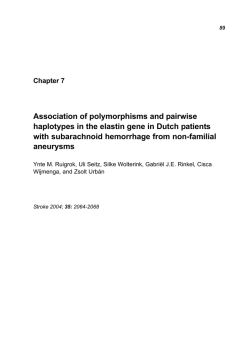
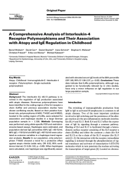
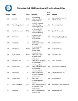

© Copyright 2026