
Download E-book (PDF)
International Journal of Physical Sciences Volume 10 Number 2 30 January, 2015 ISSN 1992-1950 ABOUT IJPS The International Journal of Physical Sciences (IJPS) is published weekly (one volume per year) by Academic Journals. International Journal of Physical Sciences (IJPS) is an open access journal that publishes high-quality solicited and unsolicited articles, in English, in all Physics and chemistry including artificial intelligence, neural processing, nuclear and particle physics, geophysics, physics in medicine and biology, plasma physics, semiconductor science and technology, wireless and optical communications, materials science, energy and fuels, environmental science and technology, combinatorial chemistry, natural products, molecular therapeutics, geochemistry, cement and concrete research, metallurgy, crystallography and computer-aided materials design. All articles published in IJPS are peer-reviewed. Contact Us Editorial Office: [email protected] Help Desk: [email protected] Website: http://www.academicjournals.org/journal/IJPS Submit manuscript online http://ms.academicjournals.me/ Editors Prof. Sanjay Misra Department of Computer Engineering, School of Information and Communication Technology Federal University of Technology, Minna, Nigeria. Prof. Songjun Li School of Materials Science and Engineering, Jiangsu University, Zhenjiang, China Dr. G. Suresh Kumar Senior Scientist and Head Biophysical Chemistry Division Indian Institute of Chemical Biology (IICB)(CSIR, Govt. of India), Kolkata 700 032, INDIA. Dr. 'Remi Adewumi Oluyinka Senior Lecturer, School of Computer Science Westville Campus University of KwaZulu-Natal Private Bag X54001 Durban 4000 South Africa. Prof. Hyo Choi Graduate School Gangneung-Wonju National University Gangneung, Gangwondo 210-702, Korea Prof. Kui Yu Zhang Laboratoire de Microscopies et d'Etude de Nanostructures (LMEN) Département de Physique, Université de Reims, B.P. 1039. 51687, Reims cedex, France. Prof. R. Vittal Research Professor, Department of Chemistry and Molecular Engineering Korea University, Seoul 136-701, Korea. Prof Mohamed Bououdina Director of the Nanotechnology Centre University of Bahrain PO Box 32038, Kingdom of Bahrain Prof. Geoffrey Mitchell School of Mathematics, Meteorology and Physics Centre for Advanced Microscopy University of Reading Whiteknights, Reading RG6 6AF United Kingdom. Prof. Xiao-Li Yang School of Civil Engineering, Central South University, Hunan 410075, China Dr. Sushil Kumar Geophysics Group, Wadia Institute of Himalayan Geology, P.B. No. 74 Dehra Dun - 248001(UC) India. Prof. Suleyman KORKUT Duzce University Faculty of Forestry Department of Forest Industrial Engineeering Beciyorukler Campus 81620 Duzce-Turkey Prof. Nazmul Islam Department of Basic Sciences & Humanities/Chemistry, Techno Global-Balurghat, Mangalpur, Near District Jail P.O: Beltalapark, P.S: Balurghat, Dist.: South Dinajpur, Pin: 733103,India. Prof. Dr. Ismail Musirin Centre for Electrical Power Engineering Studies (CEPES), Faculty of Electrical Engineering, Universiti Teknologi Mara, 40450 Shah Alam, Selangor, Malaysia Prof. Mohamed A. Amr Nuclear Physic Department, Atomic Energy Authority Cairo 13759, Egypt. Dr. Armin Shams Artificial Intelligence Group, Computer Science Department, The University of Manchester. Editorial Board Prof. Salah M. El-Sayed Mathematics. Department of Scientific Computing. Faculty of Computers and Informatics, Benha University. Benha , Egypt. Prof. Mohammed H. T. Qari Department of Structural geology and remote sensing Faculty of Earth Sciences King Abdulaziz UniversityJeddah, Saudi Arabia Dr. Rowdra Ghatak Associate Professor Electronics and Communication Engineering Dept., National Institute of Technology Durgapur Durgapur West Bengal Dr. Jyhwen Wang, Department of Engineering Technology and Industrial Distribution Department of Mechanical Engineering Texas A&M University College Station, Prof. Fong-Gong Wu College of Planning and Design, National Cheng Kung University Taiwan Dr. Abha Mishra. Senior Research Specialist & Affiliated Faculty. Thailand Dr. Madad Khan Head Department of Mathematics COMSATS University of Science and Technology Abbottabad, Pakistan Prof. Yuan-Shyi Peter Chiu Department of Industrial Engineering & Management Chaoyang University of Technology Taichung, Taiwan Dr. M. R. Pahlavani, Head, Department of Nuclear physics, Mazandaran University, Babolsar-Iran Dr. Subir Das, Department of Applied Mathematics, Institute of Technology, Banaras Hindu University, Varanasi Dr. Anna Oleksy Department of Chemistry University of Gothenburg Gothenburg, Sweden Prof. Gin-Rong Liu, Center for Space and Remote Sensing Research National Central University, Chung-Li, Taiwan 32001 Prof. N. V. Sastry Department of Chemistry Sardar Patel University Vallabh Vidyanagar Gujarat, India Dr. Edilson Ferneda Graduate Program on Knowledge Management and IT, Catholic University of Brasilia, Brazil Dr. F. H. Chang Department of Leisure, Recreation and Tourism Management, Tzu Hui Institute of Technology, Pingtung 926, Taiwan (R.O.C.) Prof. Annapurna P.Patil, Department of Computer Science and Engineering, M.S. Ramaiah Institute of Technology, Bangalore-54, India. Dr. Ricardo Martinho Department of Informatics Engineering, School of Technology and Management, Polytechnic Institute of Leiria, Rua General Norton de Matos, Apartado 4133, 2411901 Leiria, Portugal. Dr Driss Miloud University of mascara / Algeria Laboratory of Sciences and Technology of Water Faculty of Sciences and the Technology Department of Science and Technology Algeria International Journal of Physical Sciences Table of Contents: Volume 10 Number 2, 30 January, 2015 ARTICLES On the hydrogenation-dehydrogenation of graphene-layer-nanostructures: Relevance to the hydrogen on-board storage problem Yu S. Nechaev and Nejat T. Veziroglu Recent astronomical tests of general relativity Keith John Treschman 54 90 Vol. 10(2), pp. 54-89, 30 Janaury, 2015 DOI: 10.5897/IJPS2014.4212 Article Number: 3E9497250049 ISSN 1992 - 1950 Copyright ©2015 Author(s) retain the copyright of this article http://www.academicjournals.org/IJPS International Journal of Physical Sciences Full Length Research Paper On the hydrogenation-dehydrogenation of graphenelayer-nanostructures: Relevance to the hydrogen onboard storage problem Yu S. Nechaev1* and Nejat T. Veziroglu2 1 Bardin Institute for Ferrous Metallurgy, Kurdjumov Institute of Metals Science and Physics, Vtoraya Baumanskaya St., 9/23, Moscow 105005, Russia. 2 International Association for Hydrogen Energy, 5794 SW 40 St. #303, Miami, FL 33155, USA. Received 15 September, 2014; Accepted 1 December, 2014 Herein, results of thermodynamic analysis of some theoretical and experimental [thermal desorption (TDS), scanning tunneling microscopy (STM), scanning tunneling spectroscopy (STS), high-resolution electron energy loss spectroscopy/low-energy electron diffraction (HREELS/LEED), photoelectron spectroscopy (PES), angle-resolved photoemission spectroscopy (ARPES), Raman spectroscopy and others] data on “reversible” hydrogenation and dehydrogenation of some graphene-layernanostructures are presented. In the framework of the formal kinetics and the approximation of the first order rate reaction, some thermodynamic quantities for the reaction of hydrogen sorption (the reaction rate constant, the reaction activation energy, the per-exponential factor of the reaction rate constant) have been determined. Some models and characteristics of hydrogen chemisorption on graphite (on the basal and edge planes) have been used for interpretation of the obtained quantities, with the aim of revealing the atomic mechanisms of hydrogenation and dehydrogenation of different graphene-layersystems. The cases of both non-diffusion rate limiting kinetics and diffusion rate limiting kinetics are considered. Some open questions and perspectives remain in solving the actual problem in effective hydrogen on-board storage; using the graphite nanofibers (GNFs) is also considered. Key words: Epitaxial and membrane graphenes, other graphene-layer-systems, hydrogenationdehydrogenation, thermodynamic characteristics, atomic mechanisms, the hydrogen on-board efficient storage problem. INTRODUCTION As noted in a number of articles 2007 through 2014, hydrogenation of graphene-layers-systems, as a prototype of covalent chemical functionality and an effective tool to open the band gap of graphene, is of both fundamental and applied importance (Geim and Novoselov, 2007; Palerno, 2013). It is relevant to the current problems of thermodynamic stability and thermodynamic characteristics of the hydrogenated graphene-layers-systems (Sofo et al., 2007; Openov and Podlivaev, 2010; Han et al., 2012), and also to the current problem of hydrogen on-board storage (Akiba, 2011; Zuettel, 2011; DOE targets, 2012). *Corresponding author. E-mail: [email protected] Author(s) agree that this article remain permanently open access under the terms of the Creative Commons Attribution License 4.0 International License Nechaev and Veziroglu In the case of epitaxial graphene on substrates, such as SiO2 and others, hydrogenation occurs only on the top basal plane of graphene, and it is not accompanied with a strong (diamond-like) distortion of the graphene network, but only with some ripples. The first experimental indication of such a specific single-side hydrogenation came from Elias et al. (2009). The authors mentioned a possible contradiction with the theoretical results of Sofo et al. (2007), which had down-played the possibility of a single side hydrogenation. They proposed an important facilitating role of the material ripples for hydrogenation of graphene on SiO2, and believed that such a single-side hydrogenated epitaxial graphene can be a disordered material, similar to graphene oxide, rather than a new graphene-based crystal - the experimental graphane produced by them (on the free-standing graphene membrane). On the other hand, it is expedient to note that changes in Raman spectra of graphene caused by hydrogenation were rather similar (with respect to locations of D, G, D′, 2D and (D+D′) peaks) both for the epitaxial graphene on SiO2 and for the free-standing graphene membrane (Elias et al., 2009). As it is supposed by many scientists, such a single side hydrogenation of epitaxial graphene occurs, because the diffusion of hydrogen along the graphene-SiO2 interface is negligible, and perfect graphene is impermeable to any atom and molecule (Jiang et al., 2009). But, firstly, these two aspects are of the kinetic character, and therefore they cannot influence the thermodynamic predictions (Sofo et al., 2007; Boukhvalov et al., 2008; Zhou et al., 2009). Secondly, as shown in the present analytical study, the above noted two aspects have not been studied in an enough degree. As shown in Elias et al. (2009), when a hydrogenated graphene membrane had no free boundaries (a rigidly fixed membrane) in the expanded regions of it, the lattice was stretched isotropically by nearly 10%, with respect to the pristine graphene. This amount of stretching (10%) is close to the limit of possible elastic deformations in graphene (Nechaev and Veziroglu, 2013), and indeed it has been observed that some of their membranes rupture during hydrogenation. It was believed (Elias et al., 2009) that the stretched regions were likely to remain nonhydrogenated. They also found that instead of exhibiting random stretching, hydrogenated graphene membranes normally split into domain-like regions of the size of the order of 1 μm, and that the annealing of such membranes led to complete recovery of the periodicity in both stretched and compressed domains (Elias et al., 2009). It can be supposed that the rigidly fixed graphene membranes are related, in some degree, to the epitaxial graphenes. Those may be rigidly fixed by the cohesive interaction with the substrates. As was noted in Xiang et al. (2010), the double-side hydrogenation of graphene is now well understood, at least from a theoretical point of view. For example, Sofo 55 et al. (2007) predicted theoretically a new insulating material of CH composition called graphane (double-side hydrogenated graphene), in which each hydrogen atom adsorbs on top of a carbon atom from both sides, so that the hydrogen atoms adsorbed in different carbon sublattices are on different sides of the monolayer plane (Sofo et al., 2007). The formation of graphane was 3 attributed to the efficient strain relaxation for sp hybridization, accompanied by a strong (diamond-like) distortion of the graphene network (Sofo et al., 2007; Xiang et al., 2009). In contrast to graphene (a zero-gap semiconductor), graphane is an insulator with an energy gap of Eg| 5.4 eV (Openov and Podlivaev, 2010; Lebegue et al., 2009). Only if hydrogen atoms adsorbed on one side of graphene (in graphane) are retained, we obtain graphone of C2H composition, which is a magnetic semiconductor with Eg| 0.5 eV, and a Curie temperature of Tc| 300 to 400K (Zhou et al., 2009). As was noted in Openov and Podlivaev (2012), neither graphone nor graphane are suitable for real practical applications, since the former has a low value of Eg, and undergoes a rapid disordering because of hydrogen migration to neighboring vacant sites even at a low temperature, and the latter cannot be prepared on a solid substrate (Podlivaev and Openov, 2011). It is also expedient to refer to a theoretical single-side hydrogenated graphene (SSHG) of CH composition (that is, an alternative to graphane (Sofo et al. (2007)), in which hydrogen atoms are adsorbed only on one side (Pujari et al., 2011; Dzhurakhalov and Peeters, 2011). In contrast to graphone, they are adsorbed on all carbon atoms rather than on every second carbon atom. The value of Eg in SSHG is sufficiently high (1.6 eV lower than in graphane), and it can be prepared on a solid substrate in principle. But, this quasi-two-dimensional carbonhydrogen theoretical system is shown to have a relatively low thermal stability, which makes it difficult to use SSGG in practice (Openov and Podlivaev, 2012; Pujari et al., 2011). As was noted in Pujari et al. (2011), it may be inappropriate to call the covalently bonded SSHG system 3 sp hybridized, since the characteristic bond angle of 109.5° is not present anywhere that is, there is no diamond-like strong distortion of the graphene network, rather than in graphane. Generally in the case of a few hydrogen atoms interacting with graphene or even for graphane, the underlining carbon atoms are displaced from their locations. For instance, there may be the diamond-like local distortion of the graphene network, 3 showing the signature of sp bonded system. However, in SSHGraphene all the carbon atoms remain in one plane, making it difficult to call it sp3 hybridized. Obviously, this 3 is some specific sp - like hybridization. The results of Nechaev (2010), and also Table 1A and B in the present paper, of thermodynamic analysis of a number of experimental data point that some specific Int. J. Phys. Sci. Rigidly fixed hydrogenated graphene membrane (Elias et al., 2009) Diamond (Nechaev and Veziroglu, 2013) Graphite (Nechaev and Veziroglu, 2013) 3.69 ± 0.02 (analysis) There are no experimental values in the work Hydrogenated epitaxial* graphene, TDS-peak #3 (Elias et al., 2009) 7.38 ± 0.04 (analysis) 2.4 (or 0.8-7) (L~dsample) (analysis) 0.23 ± 0.05 (as process ~I,~ models “F”,“G”, Figure 4) (analysis) Hydrogenated epitaxial* graphene, TDS-peak #2 (Elias et al., 2009) 4.93 (analysis) 4.94 ± 0.03 (analysis) 1 × 10⁶ (or 4 × 10² - 2 × 10⁹) (L~dsample) (analysis) 0.6 ± 0.3 (as for processes ~I-II, ~model “G”, Figure 4) (analysis) Hydrogenated epitaxial* graphene, TDS-peak #1 (Elias et al., 2009) 7.40 (theory) 7.41 ± 0.05 (analysis) 2 × 10⁷ (or 2 × 1032 × 1011) (L~ dsample) (analysis) 0.6 ± 0.3 (as processes ~ I-II,~ model “G”, Figure 4) (analysis) There are no experimental values in the work Hydrogenated epitaxial graphene (Elias et al., 2009) Graphene (Dzhurakhalov and Peeters, 2011) if 7 × 10¹² if 5 × 10¹³ then 0.2 then 80 then 3.5 × 10⁴ (K0(ads.) ≈ K0(des.)) (L~dsample) then 1.84 then 1.94 if 0.3 if 0.6 if 0.9 (0.3 ± 0.2) (analysis) There are no experimental values in the work then 7 × 10¹² then 5 × 10¹³ (K0(ads.) ≈ K0(des.)) if 2.5 ± 0.1 if 2.6 ± 0.1 (1.0 ± 0.2) (analysis ) There are no experimental values in the work Free-standing graphene-like membrane (Elias et al., 2009) There are no experimental values in the work 2.0 × 10¹⁵ (analysis) K0(des.), s-1 (L ≈(D0app./K0(des.))1/2) 2.46 ± 0.17 (theory) ∆H(des.) (eV) ∆H(ads.) (eV) 2.46 ± 0.17 (analysis) 2.7 (analysis) 2.35 (analysis) ∆H(C-C), (eV) Graphane CH (Openov and Podlivaev, 2010) 6.56 (theory) 5.03 (theory) ∆H(bind.), eV 2.5 ± 0.1(analysis) 1.50 (theory) ∆H(C-H) (eV) Graphane CH (Sofo et al. , 2007) Graphane CH (Dzhurakhalov and Peeters, 2011) Material Value/quantity Table 1A. Theoretical, experimental and analytical values of some related quantities. 56 2.40 ± 0.05 [analysis, process I, models “F”, “G” (Figure 4)] 3.77 ± 0.05 [analysis, process IV, models “C”, “D” (Figure 4)] Hydrogenated isotropic graphite, carbon nanotubes (Nechaev, 2010) Hydrogenated isotropic and pyrolytic and nanostructured graphite (Nechaev, 2010) 4.94 ± 0.03 (analysis) There are empirical values in the work (analysis of experiment) There are empirical values in the work (analysis of experiment) 0.21 ± 0.02 (analysis, process I) 3.8 ± 0.5 (analysis, process IV) 57 graphenes is possible and even reversible, and why the hydrogenated species are stable at room temperatures (Elias et al., 2009; Sessi et al., 2009). This puzzling situation is also considered in the present analytical study. Xiang et al. (2010) noted that their test calculations show that the barrier for the penetration of a hydrogen atom through the sixmember ring of graphene is larger than 2.0 eV. Thus, they believe that it is almost impossible for a hydrogen atom to pass through the six-member ring of graphene at room temperature (from a There are empirical values in thework (analysis of experiment) There are empirical values in the work (analysis of experiment) K0(des.), s-1 1.24 ± 0.03 (analysis, process II) 2.6 ± 0.03 (analysis, process III) Value/quantity ∆H(C-C), eV ∆H(des.), eV that hydrogen chemisorption corrugates the graphene sheet in fullerene, carbon nanotubes, graphite and graphene, and transforms them from a semimetal into a semiconductor (Sofo et al., 2007; Elias et al., 2009). This can even induce magnetic moments (Yazyev and Helm, 2007; Lehtinen et al., 2004; Boukhvalov et al., 2008). Previous theoretical studies suggest that singleside hydrogenation of ideal graphene would be thermodynamically unstable (Boukhvalov et al., 2008; Zhou et al., 2009). Thus, it remains a puzzle why the single-side hydrogenation of epitaxial 2.90 ± 0.05 [analysis, process II, models “H”,“G” (Figure 4)] Hydrogenated isotropic graphite, graphite nano-fibers, nanostructured graphite, defected carbon nanotubes (Nechaev, 2010) local sp3- like hybridization, without the diamondlike strong distortion of the graphene network, may be manifested itself in the cases of hydrogen atoms dissolved between graphene layers in isotropic graphite, graphite nanofibers (GNFs) and nanostructured graphite, where obviously there is a situation similar (in a definite degree) to one of the rigidly fixed graphene membranes. As far as we know, it has not been taken into account in many recent theoretical studies. In this connection, it is expedient to note that there are a number of theoretical works showing 2.50 ± 0.03 (analysis, process III, model “F*”) 2.5 ± 0.2 (theory) ∆H(C-H) , eV 2.64 ± 0.01 (experiment) Hydrogenated isotropic graphite, graphite nanofibers and nanostructured graphite(Nechaev, 2010) Hydrogenated carbon nanotubes C2H(Bauschlicher and So, 2002) Hydrofullerene C60H36 (Pimenova et al., 2002) Material Table 1B. Theoretical, experimental and analytical values of some related quantities. Nechaev and Veziroglu 58 Int. J. Phys. Sci. Figure 1. Structure of the theoretical graphane in chair configuration. The carbon atoms are shown in gray and the hydrogen atoms in white. The figure shows the diamond-like distorted hexagonal network with carbon in sp3 hybridization (Sofo et al., 2007). private communication with Xiang et al. (2009). In the present analytical study, a real possibility of the penetration is considered when a hydrogen atom can pass through the graphene network at room temperature. This is the case of existing relevant defects in graphene, that is, grain boundaries, their triple junctions (nodes) and/or vacancies (Brito et al., 2011; Zhang et al., 2014; Banhart et al., 2011; Yazyev and Louie, 2010; Kim et al., 2011; Koepke et al., 2013; Zhang and Zhao, 2013; Yakobson and Ding, 2011; Cockayne et al., 2011; Zhang et al., 2012; Eckmann et al., 2012). The present study is related to revealing the atomic mechanisms of reversible hydrogenation of epitaxial graphenes, compared with membrane graphenes. In the next parts of this paper, results of thermodynamic analysis, comparison and interpretation of some theoretical and experimental data are presented, which are related to better understanding and/or solving of the open questions mentioned above. It is related to a further development and modification of our previous analytical results (2010-2014), particularly published in the openaccess journals. Therefore, in the present paper, the related figures 1- 25 from our “open” publication (Nechaev and Veziroglu, 2013) are referred. has been predicted on the basis of the first principles and total-energy calculations. All of the carbon atoms are in 3 sp hybridization forming a hexagonal network (a strongly diamond-like distorted graphene network) and the hydrogen atoms are bonded to carbon on both sides of the plane in an alternative manner. It has been found that graphane can have two favorable conformations: a chairlike (diamond-like, Figure 1) conformer and a boat-like (zigzag-like) conformer (Sofo et al., 2007). The diamond-like conformer (Figure 1) is more stable than the zigzag-like one. This was concluded from the results of the calculations of binding energy (∆Hbind.(graphane)) (that is, the difference between the total energy of the isolated atoms and the total energy of the compounds), and the standard energy of formation 0 (∆H f298(graphane)) of the compounds (CH(graphane)) from crystalline graphite (C(graphite)) and gaseous molecular and hydrogen (H2(gas)) at the standard pressure temperature conditions (Sofo et al., 2007; Dzhurakhalov and Peeters, 2011). For the diamond-like graphane, the former quantity is ∆Hbind.(graphane) = 6.56 eV/atom, and the latter one is ∆H1 = ∆H0f298(graphane) = - 0.15 eV/atom. The latter quantity corresponds to the following reaction: C(graphite) + ½H2(gas)→ CH(graphane), CONSIDERATION OF SOME ENERGETIC CHARACTERISTICS OF THEORETICAL GRAPHANES In the work of Sofo et al. (2007), the stability of graphane, a fully saturated extended two-dimensional hydrocarbon derived from a single grapheme sheet with formula CH, (∆H1) (1) Where ∆H1 is the standard energy (enthalpy) change for this reaction. By using the theoretical quantity of ∆H0f298(graphane), one can evaluate, using the framework of the thermodynamic method of cyclic processes (Karapet’yants and Nechaev and Veziroglu Karapet’yants, 1968; Bazarov, 1976), a value of the energy of formation (∆H2) of graphane (CH(graphane)) from graphene (C(graphene)) and gaseous atomic hydrogen (H(gas)). For this, it is necessary to take into consideration the following three additional reactions: C(graphene)+ H(gas)→ CH(graphane),(∆H2) (2) C(graphene)→ C(graphite), (∆H3) (3) H(gas)→ ½ H2(gas), (H4) (4) where ∆H2, ∆H3 and ∆H4 are the standard energy (enthalpy) changes. Reaction 2 can be presented as a sum of Reactions 1, 3 and 4 using the framework of the thermodynamic method of cyclic processes (Bazarov, 1976): ∆H2 = (∆H3+∆H4+∆H1). 59 generation reactive empirical bond order of Brenner interatomic potential. As shown, the cohesive energy of graphane (CH) in the ground state is ∆Hcohes.(graphane) = 5.03 eV/atom (C). This results in the binding energy of hydrogen, which is ∆H(C-H)graphane = 1.50 eV/atom (Dzhurakhalov and Peeters, 2011) (Table 1A). The theoretical ∆Hbind.(graphane) quantity characterizes the 3 3 breakdown energy of one C-H sp bond and 1.5 C-C sp bonds (Figure 1). Hence, by using the above mentioned values of ∆Hbind.(graphane) and ∆H(C-H)graphane, one can 3 evaluate the breakdown energy ofC-C sp bonds in the theoretical graphane (Sofo et al., 2007), which is ∆H(CC)graphane = 2.7 eV (Table 1). Also, by using the above noted theoretical values of ∆Hcohes.(graphane) and ∆H(CH)graphane, one can evaluate similarly the breakdown energy ofC-C sp3 bonds in the theoretical graphane (Dzhurakhalov and Peeters, 2011), which is ∆H(C-C)graphane = 2.35 eV (Table 1A). (5) Substituting in Equation 5 the known experimental values (Karapet’yants and Karapet’yants, 1968; Dzhurakhalov and Peeters, 2011) of ∆H4 = -2.26 eV/atom and ∆H3 = 0.05 eV/atom, and also the theoretical value (Sofo et al., 2007) of ∆H1 = -0.15 эВ/atom, one can obtain a desired value of ∆H2 = -2.5 ± 0.1 eV/atom. The quantity of -∆H2 characterizes the breakdown energy ofC-H sp3 bond in graphane (Figure 1), relevant to the breaking away of one hydrogen atom from the material, which is ∆H(C-H)graphane = -∆H2 = 2.5 ± 0.1 eV (Table 1A). In evaluating the above mentioned value of ∆H3, one can use the experimental data (Karapet’yants and Karapet’yants, 1968) on the graphite sublimation energy at 298K (∆Hsubl.(graphite) = 7.41 ± 0.05 eV/atom), and the theoretical data (Dzhurakhalov and Peeters, 2011) on the binding cohesive energy at about 0K for graphene (∆Hcohes.(graphene) = 7.40 eV/atom). Therefore, neglecting the temperature dependence of these quantities in the interval of 0 to 298K, one obtains the value of ∆H3| -0.05 eV/atom. ∆Hcohes.(graphene) quantity characterizes the breakdown 2 energy of1.5 C-C sp bond in graphene, relevant to the breaking away of one carbon atom from the material. Consequently, one can evaluate the breakdown energy 2 ofC-C sp bonds in graphene, which is ∆H(C-C)grapheme = 4.93 eV. This theoretical quantity coincides with the similar empirical quantities obtained in (Nechaev and 2 Veziroglu, 2013) from ∆Hsubl.(graphite) forC-C sp bonds in graphene and graphite, which are ∆H(C-C)graphene | ∆H(CC)graphite = 4.94 ± 0.03 eV. The similar empirical quantity for C-C sp3 bonds in diamond obtained from the diamond sublimation energy ∆Hsubl.(diamond) (Karapet’yants and Karapet’yants, 1968) is ∆H(C-C)diamond = 3.69 ± 0.02 eV (Nechaev and Veziroglu, 2013). It is important to note that chemisorption of hydrogen on graphene was studied (Dzhurakhalov and Peeters, 2011) using atomistic simulations, with a second CONSIDERATION AND INTERPRETATION OF THE DATA ON DEHYDROGENATION OF THEORETICAL GRAPHANE, COMPARING WITH THE RELATED EXPERIMENTAL DATA In Openov and Podlivaev (2010) and Elias et al. (2009) the process of hydrogen thermal desorption (TDS) from graphane has been studied using the method of molecular dynamics. The temperature dependence (for T = 1300 - 3000K) of the time (t0.01) of hydrogen desorption onset (that is, the time t0.01 of removal a1% of the initial hydrogen concentration C0 | 0.5 (in atomic fractions), ΔC/C0 | 0.01, C/C0| 0.99) from the C54H7(54+18) clustered with 18 hydrogen passivating atoms at the edges to saturate the dangling bonds of sp3-hybridized carbon atoms have been calculated. The corresponding activation energy of ∆H(des.) = Ea = 2.46 ± 0.17 eV and the corresponding (temperature independent) frequency 17 -1 factor A = (2.1 ± 0.5) × 10 s have also been calculated. The process of hydrogen desorption at T = 1300 - 3000K has been described in terms of the Arrhenius-type relationship: 1/t0.01 = A exp (-Ea /kB T), (6) where kB is the Boltzmann constant. Openov and Podlivaev (2010) predicted that their results would not contradict the experimental data (Elias et al., 2009), according to which the nearly complete 0.9, C/C0 | 0.1) from a desorption of hydrogen (-ΔC/C0 free-standing graphane membrane (Figure 2B) was achieved by annealing it in argon at T = 723K for 24 h 4 (that is, t0.9(membr. [5]) 723K = 8.6 × 10 s). However, as the analysis presented below shows, this declaration (Openov and Podlivaev, 2010) is not enough adequate. By using Equation (6), Openov and Podlivaev, 2010) evaluated the quantity of t0.01(graphane[4]) for T = 300K 60 Int. J. Phys. Sci. 24 3 (a110 s)and for T = 600K (a2 × 10 s). However, they noted that the above two values of t0.01(graphane) should be considered as rough estimates. Indeed, using Equation 6, one can evaluate the value of t0.01(graphane[4])723K| 0.7 s for T = 723K, which is much less (by five orders) than the t0.9(membr.[5])723K value in Elias et al. (2009). In the framework of the formal kinetics approximation in the first order rate reaction (Bazarov, 1976) a characteristic quantity for the reaction of hydrogen desorption is W0.63 - the time of the removal of ~ 63% of the initial hydrogen concentration C0 (that is, -ΔC/C0| 0.63, C/C0| 0.37) from the hydrogenated graphene. Such a first order rate reaction (desorption) can be described by the following equations (Nechaev, 2010; Nechaev and Veziroglu, 2013; Bazarov, 1976): dC / dt = - KC, (7) (C / C0) = exp (- Kt ) = exp (- t /W0.63), (8) K = (1/W0.63) = K0 exp (-ΔHdes./ kB T ), (9) Where C is the averaged concentration at the annealing time t, K = (1/W0.63) is the reaction (desorption) rate constant, ΔHdes.is the reaction (desorption) activation energy, and K0, the per-exponential (or frequency) factor of the reaction rate constant. In the case of a diffusion rate limiting kinetics, the quantity of K0 is related to a solution of the corresponding 2 diffusion problem (K0 ≈ D0 /L , where D0 is the perexponential factor of the diffusion coefficient, L is the characteristic diffusion length) (Nechaev, 2010; Nechaev and Veziroglu, 2013). In the case of a non-diffusion rate limiting kinetics, which is obviously related to the situation of Openov and Podlivaev (2010) and Elias et al. (2009), the quantity of K0 may be the corresponding vibration (for (C-H) bonds) frequency (K0 = Q(C-H)), the quantity ΔH(des.) = ΔH(C-H) (Table 1), and Equation (9) corresponds to PolanyiWigner (Nechaev, 2010; Nechaev and Veziroglu, 2013). By substituting in Equation (8) the quantities of t = t0.01(graphane[4])723K and (C/C0) = 0.99, one can evaluate the desired quantity W0.63(graphane[4])723K| 70 s. Analogically, the quantity of t0.9(graphane[4])723K| 160 s can be evaluated, which is less by about three orders - than the experimental value (Elias et al., 2009) of t0.9(membr.[5])723K. In the same manner, one can evaluate the desired 4 quantity W0.63(membr.[5])723K|3.8 ×10 s, which is higher (by about three orders) than W0.63(graphane[4])723K. By using Equation (9) and supposing that ΔHdes.= Ea and K = 1/W0.63(graphane[4])723K, one can evaluate the 15 -1 analytical quantity of K0(graphane[4]) = 2 × 10 s for graphane of (Openov and Podlivaev, 2010) (Table 1A). By substituting in Equation (9) the quantity of K = K(membr.[5])723K = 1/W0.63(membr.[5])723K and supposing that ΔHdes.(membr.[5]) | ∆HC-H(graphane[3,4]) | 2.5 eV (Sofo et al., 2007; Nechaev and Veziroglu, 2013; Openov and Podlivaev, 2010) (Table 1A), one can evaluate the 12 -1 quantity of K0(membr.[5]) = Q(membr.[5])| 7 × 10 s for the experimental graphane membranes of Elias et al. (2009). The obtained quantity of Q(membr.[5]) is less by one and a 14 half orders of the vibrational frequency QRD = 2.5 × 10 s -1 1 , corresponding to the D Raman peak (1342 cm ) for hydrogenated graphene membrane and epitaxial graphene on SiO2 (Figure 2). The activation of the D Raman peak in the hydrogenated samples authors (Elias et al., 2009) attribute to breaking of the translation 2 3 symmetry of C-C sp bonds after formation of C-H sp bonds. The quantity Q(membr.[5]) is less by one order of the value (Xie et al., 2011) of the vibration frequency QHREELS = 8.7 13 -1 × 10 s corresponding to an additional HREELS peak arising from C-H sp3 hybridization; a stretching appears at 369 meV after a partial hydrogenation of the epitaxial graphene. Xie et al. (2011) suppose that this peak can be assigned to the vertical C-H bonding, giving direct evidence for hydrogen attachment on the epitaxial graphene surface. Taking into account QRD and QHREELS quantities, and substituting in Equation (9) quantities of K = 1/W0.63(membr.[5])723K and K0|K0(membr.[5])|QHREELS, one can evaluate ΔHdes.(membr.[5])= ∆HC-H(membr.[5]) | 2.66 eV (Table 1A). In such approximation, the obtained value of ∆HCcoincides (within the errors) with the H(membr.[5]) experimental value (Pimenova et al., 2002) of the breakdown energy of C-H bonds in hydrofullerene C60H36 (∆HC-H(C60H36) = 2.64 ± 0.01 eV, Table 1B). The above analysis of the related data shows that the experimental graphene membranes (hydrogenated up to the near-saturation) can be used. The following thermodesorption characteristics of the empirical character, relevant to Equation (9): ΔHdes.(membr.[5])= ∆HCH(membr.[5]) = 2.6 ± 0.1 eV, K0(membr.[5]) = QC-H(membr.[5])| 5 × 13 -1 10 s (Table 1A). The analysis also shows that this is a case for a non-diffusion rate limiting kinetics, when Equation (9) corresponds to Polanyi-Wigner (Nechaev, 2010; Nechaev and Veziroglu, 2013). Certainly, these tentative results could be directly confirmed and/or modified by receiving and treating within Equations (8) and (9) of the experimental data on W0.63 at several annealing temperatures. The above noted fact that the empirical (Elias et al., 2009; Nechaev and Veziroglu, 2013) quantity W0.63(membr.[5])723K is much larger (by about 3 orders), than the theoretical (Openov and Podlivaev, 2010; Nechaev and Veziroglu, 2013) one (W0.63(graphane[4])723K), is consistent with that mentioned in (Elias et al., 2009). The alternative possibility has been supposed in Elias et al., (2009) that (i) the experimental graphane membrane (a free-standing one) may have “a more complex hydrogen bonding, than the suggested by the theory”, and that (ii) graphane (CH) (Sofo et al., 2007) may be until now the theoretical material. Nechaev and Veziroglu 61 Figure 2. Changes in Raman spectra of graphene caused by hydrogenation (Elias et al., 2009). The spectra are normalized to have a similar integrated intensity of the G peak. (A) Graphene on SiO2. (B) Free-standing graphene. Red, blue, and green curves (top to bottom) correspond to pristine, hydrogenated, and annealed samples, respectively. Graphene was hydrogenated for a2 hours, and the spectra were measured with a Renishaw spectrometer at wavelength 514 nm and low power to avoid damage to the graphene during measurements. (Left inset) Comparison between the evoluation of D and D′ peaks for single- and double-sided exposure to atomic hydrogen. Shown is a partially hydrogenated state achieved after 1 hour of simultaneous exposure of graphene on SiO2 (blue curve) and of a membrane (black curve). (Right inset) TEM image of one of the membranes that partially covers the aperture 50 μm in diameter. CONSIDERATION OF THE EXPERIMENTAL DATA ON HYDROGENATION-DEHYDROGENATION OF MONOAND BI-LAYER EPITAXIAL GRAPHENES, AND COMPARING THE RELATED DATA FOR FREESTANDING GRAPHENE Characteristics of hydrogenation-dehydrogenation of mono-layer epitaxial graphenes In Elias et al. (2009), both the graphene membrane samples considered above, and the epitaxial graphene and bi-graphene samples on substrate SiO2 were exposed to cold hydrogen DC plasma for 2 h to reach the saturation in the measured characteristics. They used a low-pressure (0.1 mbar) hydrogen-argon mixture of 10% H2. Raman spectra for hydrogenated and subsequently annealed free-standing graphene membranes (Figure 2B) are rather similar to those for epitaxial graphene samples (Figure 2A), but with some notable differences. If hydrogenated simultaneously for 1 h, and before reaching the saturation (a partial hydrogenation), the D peak area for a free-standing membrane is two factors greater than the area for graphene on a substrate (Figure 2, the left inset). This indicates the formation of twice as 3 many C-H sp bonds in the membrane. This result also agrees with the general expectation that atomic hydrogen attaches to both sides of the membranes. Moreover, the D peak area became up to about three times greater than the G peak area after prolonged exposures (for 2 h, a near-complete hydrogenation) of the membranes to atomic hydrogen. The integrated intensity area of the D peak in Figure 2B corresponding to the adsorbed hydrogen saturation concentration in the graphene membranesis larger by a factor of about 3 for the area of the D peak in Figure 2A, corresponding to the hydrogen concentration in the epitaxial graphene samples. The above noted Raman spectroscopy data (Elias et al., 2009) on dependence of the concentration (C) of adsorbed hydrogen from the hydrogenation time (t) (obviously, at about 300K) can be described with Equation (8) (Xiang et al., 2010; Bazarov, 1976). By using the above noted Raman spectroscopy data (Elias et al., 2009) (Figure 2), one can suppose that the nearsaturation ((C/C0) ≈ 0.95) time (t0.95) for the free standing graphene membranes (at ~300K) is about 3 h, and a maximum possible (but not defined experimentally) value of C0(membr.) ≈ 0.5 (atomic fraction, that is, the atomic ratio 62 Int. J. Phys. Sci. (H/C) =1). Hence, using Equation (8)* results in the quantities of W0.63(membr.[5])hydr.300K ≈ 1.0 h, C3h(membr.[5]) ≈ 0.475, C2h(membr.[5]) ≈ 0.43 and C1h(membr.[5]) ≈ 0.32, where, C3h(membr.[5]), C2h(membr.[5]) and C1h(membr.[5]) being the adsorbed hydrogen concentration at the hydrogenation time (t) equal to 3, 2 and 1 h, respectively. It is expedient to note that the quantity of C0(membr.[5]) ≈ 0.5 corresponds to the local concentration of C0(membr.[5]one_side) ≈ 0.33 for each of the two sides of a membrane, that is, the local atomic ratio (H/C) = 0.50. The evaluated value of W0.63(membr.[5])hydr.300K (for process of hydrogenation of the free standing graphene membranes (Elias et al., 2009) is much less (by about 26 orders) of the evaluated value of the similar quantity of W0.63(membr.[5])dehydr.300K ≈ (0.4 - 2.7) × 1026 h (if ∆H(des.) = (2.49 - 2.61) eV, K0(des.) = (0.7 -5) × 1013 s-1, Table 1A) for process of dehydrogenation of the same free standing graphene membranes (Elias et al., 2009). This shows that the activation energy of the hydrogen adsorption (∆H(ads.)) for the free standing graphene membranes (Elias et al., 2009) is considerably less than the activation energy of the hydrogen desorption (∆H(des.) = (2.5 or 2.6) eV). Hence, by using Equation (9) and supposing that K0(ads.) ≈ K0(des.), one can obtain a reasonable value of ∆H(ads.)membr.[5] = 1.0 ± 0.2 eV (Table 1). The heat of adsorption of atomic hydrogen by the free standing graphene membranes (Elias et al., 2009) may be evaluated as (Nechaev, 2010; Bazarov, 1976): (∆H(ads.)membr.[5] - ∆H(des.)membr.[5]) = -1.5 ± 0.2 eV (an exothermic reaction). One can also suppose that the near-saturation ((C/C0) ≈ 0.95) time (t0.95) for the epitaxial graphene samples (at ~300K) is about 2 h. Hence, by using Equation 8 and the above noted data (Elias et al., 2009) on the relative concentrations [(C1h(membr.[5]) / C1h(epitax.[5])) ≈ 2, and ((C3h(membr.[5]) / C3h(epitax.[5])) ≈ 3], one can evaluate the quantities of W0.63(epitax.[5])hydr.300K ≈ 0.7 h and C0(epitax.[5]) ≈ 0.16. Obviously, C0(epitax.[5]) is related only for one of the two sides of an epitaxial graphene layer, and the local atomic ration is (H/C) ≈ 0.19. It is considerably less (about 2.6 times) of the above considered local atomic ratio (H/C) = 0.5 for each of two sides the free standing hydrogenated graphene membranes. The obtained value of W0.63(epitax.[5])hydr.300K ≈ 0.7 h (for process of hydrogenation of the epitaxial graphene samples (Elias et al., 2009) is much less (by about two seven orders) of the evaluated values of the similar quantity for the process of dehydrogenation of the same epitaxial graphene samples (Elias et al., 2009) 2 7 (W0.63(epitax.[5])dehydr.300K ≈ (1.5 ×10 - 1.0 × 10 ) h, for ∆H(des.) = (0.3 - 0.9) eV and K0(des.) = (0.2 - 3.5 × 10⁴) s-1, Table 1A). Hence, by using Equation 9 and supposing that K0(ads.) ≈ K0(des.) (a rough approximation), one can obtain a reasonable value of ∆H(ads.)epitax.[5] ≈ 0.3 ± 0.2 eV (Table 1A). The heat of adsorption of atomic hydrogen by the free standing graphene membranes (Elias et al., 2009) may be evaluated as (Nechaev, 2010; Bazarov, 1976): (∆H(ads.)epitax.[5] - ∆H(des.)epitax.[5]) = -0.3 ± 0.2 eV (an exothermic reaction). The smaller values of C0(epitax.[5]) ≈ 0.16 and (H/C)(epitax.[5]) ≈ 0.19 (in comparison with C0(membr.[5]one_side) ≈ 0.33 and (H/C)(membr.[5]one_side) ≈ 0.50) may point to a partial hydrogenation localized in some defected nanoregions (Brito et al., 2011; Zhang et al., 2014; Banhart et al., 2011; Yazyev and Louie, 2010; Kim et al., 2011; Koepke et al., 2013; Zhang and Zhao, 2013; Yakobson and Ding, 2011; Cockayne et al., 2011; Zhang et al., 2012; Eckmann et al., 2012) for the epitaxial graphene samples (even after their prolonged (3 h) exposures, that is, after reaching their near-saturation. Similar analytical results, relevance to some other epitaxial graphenes are also presented. Characteristics of dehydrogenation of mono-layer epitaxial graphenes According to a private communication from D.C. Elias,a near-complete desorption of hydrogen (-ΔC/C0 | 0.95) from a hydrogenated epitaxial graphene on a substrate SiO2 (Figure 2A) has been achieved by annealing it in 90% Ar/10% H2 mixture at T = 573K for 2 h (that is, 3 t0.95(epitax.[5])573K = 7.2 × 10 s). Hence, by using Equation 8, 3 one can evaluate the value of W0.63(epitax.[5])573K = 2.4 × 10 s for the epitaxial graphene (Elias et al., 2009), which is about six orders less than the evaluated value of W0.63(membr.[5])573K = 1.5 × 10⁹ s for the free-standing membranes (Elias et al., 2009). The changes in Raman spectra of graphene (Elias et al., 2009) caused by hydrogenation were rather similar in respect to locations of D, G, D′, 2D and (D+D′) peaks, both for the epitaxial graphene on SiO2 and for the freestanding graphene membrane (Figure 2). Hence, one can suppose that K0(epitax.[5]) = QC-H(epitax.[5])|K0(membr.[5]) = QC13 s-1 (Table 1A). Then, by H(membr.[5])| (0.7 or 5) × 10 substituting in Equation 9 the values of K = K(epitax.[5])573K = 1/W0.63(epitax.[5])573K and K0|K0(epitax.[5])|K0(membr.[5]), one can evaluate ΔHdes.(epitax.[5])= ∆HC-H(epitax.[5]) | (1.84 or 1.94) eV (Table 1A). Here, the case is supposed of a nondiffusion-rate-limiting kinetics, when Equation 9 corresponds to thePolanyi-Wigner one (Nechaev, 2010). Certainly, these tentative thermodynamic characteristics of the hydrogenated epitaxial graphene on a substrate SiO2 could be directly confirmed and/or modified by further experimental data on W0.63(epitax.) at various annealing temperatures. It is easy to show that: 1) these analytical results (for the epitaxial graphene (Elias et al., 2009) are not consistent with the presented below analytical results for the mass spectrometry data (Figure 3, TDS peaks ## 1-3, Table 1A) on TDS of hydrogen from a specially prepared single-side (obviously, epitaxial*) graphane (Elias et al., 2009); and 2) they cannot be described in the framework of the theoretical models and characteristics of thermal Nechaev and Veziroglu 63 Figure 3. Desorption of hydrogen from single-side graphane (Elias et al., 2009). The measurments were done by using a leak detector tuned to sense molecular hydrogen. The sample was heated to 573 K (the heater was switched on at t = 10 s). Control samples (exposed to pure argon plasma) exhibited much weaker and featureless response (< 5·10-8 mbar L/s), which is attributed to desorption of water at heated surfaces and subtracted from the shown data (water molecules are ionized in the massspectrometer, which also gives rise to a small hydrogen signal). stability of SSHG (Openov and Podlivaev, 2012) or graphone (Podlivaev and Openov, 2011). According to further consideration presented below (both here and subsequently), the epitaxial graphene case (Elias et al., 2009) may be related to a hydrogen desorption case of a diffusion rate limiting kinetics, when K0zQ, and Equation (9) does not correspond to the Polanyi-Wigner one (Nechaev, 2010). By using the method of Nechaev, (2010) of treatment from the TDS spectra, relevant to the mass spectrometry data (Elias et al., 2009) (Figure 3) on TDS of hydrogen from the specially prepared single-side (epitaxial*) graphane (under heating from room temperature to 573K for 6 min), one can obtain the following tentative results: (1) The total integrated area of the TDS spectra -8 corresponds to ~10 g of desorbed hydrogen that may correlate with the graphene layer mass (unfortunately, it’s not considered in Elias et al. (2009), particularly, for evaluation of the C0 quantities); (2) The TDS spectra can be approximated by three thermodesorption (TDS) peaks (# # 1-3); (3) TDS peak # 1 (~30 % of the total area, Tmax#1 |370 K) can be characterized by the activation energy of ∆H(des.) = ETDS-peak # 1= 0.6 ± 0.3 eV and by the per-exponential 7 -1 factor of the reaction rate constant K0(TDS-peak #1)| 210 s ; (4) TDS peak # 2 (~15% of the total area, Tmax#2 | 445K) can be characterized by the activation energy ∆H(des.) = ETDS-peak #2 = 0.6 ± 0.3 eV, and by the per-exponential 6 factor of the reaction rate constant K0(TDS-peak #2)| 1 × 10 -1 s ; (5) TDS peak # 3 (~55% of the total area, Tmax#3 | 540K) can be characterized by the activation energy ∆H(des.) = ETDS-peak #3 = 0.23 ± 0.05 eV and by the per-exponential -1 factor of the reaction rate constant K0(TDS-peak #3)| 2.4 s . These analytical results (on quantities of ∆H(des.) and K0) show that all three of the above noted TDS processes (#1TDS, #2TDS and #3TDS) can not been described in the framework of the Polanyi-Wigner equation (Nechaev, 2010; Nechaev and Veziroglu, 2013) (due to the obtained low values of the K0(des.) and ∆H(des.) quantities, in comparison with the Q(C-H) and ΔH(C-H) ones). As shown below, these results may be related to a hydrogen desorption case of a diffusion-rate-limiting kinetics (Nechaev, 2010; Nechaev and Veziroglu, 2013), 2 when in Equation (9) the value of K0|D0app. / L and the value of ΔHdes.= Qapp., where D0app is the per-exponent factor of the apparent diffusion coefficient Dapp. = D0app.exp (-Qapp./kBT), Qapp. is the apparent diffusion activation energy, and L is the characteristic diffusion size (length), which (as shown below) may correlate with the sample diameter (Elias et al., 2009) (L ~ dsample ≈ 4 × 10⁻³ cm, Figure 2, Right inset). TDS process (or peak) #3TDS (Figure 3, Table 1A) may be related to the diffusion-rate-limiting TDS process (or peak) I in (Nechaev, 2010), for which the apparent diffusion activation energy is Qapp.I| 0.2 eV |ETDS-peak#3 -3 2 and D0app.I| 3 × 10 cm /s, and which is related to chemisorption models “F” and/or “G” (Figure 4). By supposing of L ~ dsample, that is, of the order of diameter of the epitaxial graphene specimens (Elias et al., 2009), one can evaluate the quantity of D0app.(TDS2 -5 peak#3) |L ∙ K0(TDS-peak#3)| 4 × 10 cm (or within the errors -5 limit, it is of (1.3 - 11) × 10 cm, for ETDS-peak #3 values 0.18 - 0.28 eV, Table 1A). The obtained values of 64 Int. J. Phys. Sci. Figure 4. Schematics of some theoretical models (ab initio molecular orbital calculations (Yang and Yang, 2002) of chemisorption of atomic hydrogen on graphite on the basal and edge planes. D0app.(TDS-peak#3) satisfactory (within one-two orders, that may be within the errors limit) correlate with the D0app.I quantity. Thus, the above analysis shows that for TDS process (or peak) # 3TDS (Elias et al., 2009), the quantity of L may be of the order of diameter (dsample) of the epitaxial* graphene samples. Within approach (Nechaev, 2010), model “F” (Figure 4) is related to a “dissociative-associative” chemisorption of molecular hydrogen on free surfaces of graphene layers of the epitaxial samples (Elias et al., 2009). Model “G” (Figure 4) is related, within (Nechaev, 2010) approach, to a “dissociative-associative” chemisorption of molecular hydrogen on definite defects in graphene layers of the epitaxial samples (Elias et al., 2009), for instance, vacancies, grain boundaries (domains) and/or triple junctions (nodes) of the grain-boundary network (Brito et al., 2011; Zhang et al., 2014; Banhart et al., 2011; Yazyev and Louie, 2010; Kim et al., 2011; Koepke et al., 2013; Zhang and Zhao, 2013; Yakobson and Ding, 2011; Cockayne et al., 2011; Zhang et al., 2012; Eckmann et al., 2012), where the dangling carbon bonds can occur. TDS processes (or peaks) #1TDS and #2TDS (Elias et al., 2009) (Table 1A) may be (in some extent) related to the diffusion-rate-limiting TDS processes (or peaks) I and II in (Nechaev, 2010). Process II is characterized by the apparent diffusion activation energy Qapp.II| 1.2 eV (that is considerably higher of quantities of ETDS-peak#1 and ETDS-peak#2) 3 2 andD0app.II| 1.810 cm /s. It is related to chemisorption model “H” (Figure 4). Within approach (Nechaev, 2010), model “H” is related (as and model “G”) to a “dissociative - associative” chemisorption of molecular hydrogen on definite defects in graphene layers of the epitaxial samples (Elias et al., 2009), for instance, vacancies, grain boundaries (domains) and/or triple junctions (nodes) of the grain-boundary network noted above, where the dangling carbon bonds can occur. By supposing the possible values of ETDS-peaks##1,2 = 0.3, 0.6 or 0.9 eV, one can evaluate the quantities of K0(TDSpeak#1) and K0(TDS-peak#2) (Table 1A). Hence, by supposing of L ~ dsample, one can evaluate the quantities of D0app.(TDSpeak#1) and D0app.(TDS-peak#2), some of them correlatewith the D0app.I quantity or with D0app.II quantity. It shows that for TDS processes (or peaks) #1TDS and #2TDS (Elias et al., 2009), the quantity of L may be of the order of diameter of the epitaxial* graphene samples. For the epitaxial graphene (Elias et al., 2009) case, supposing the values of ΔHdes.(epitax.[5])| 0.3, 0.6 or 0.9 eV results in relevant values of K0(epitax.[5]) (Table 1A). Hence, by supposing of L ~ dsample, one can evaluate the quantities of D0app.(epitax.[5]), some of them correlate with the D0app.I quantity or with D0app.II quantity. It shows that for these two processes, the quantity of L also may be of the order of diameter of the epitaxial graphene samples (Elias et al., 2009). It is important to note that chemisorption of atomic hydrogen with free-standing graphane-like membranes (Elias et al., 2009) and with the theoretical graphanes may be related to model “F*” considered in (Nechaev, 2010). Unlike model “F” (Figure 4), where two hydrogen atoms are adsorbed by two alternated carbon atoms in a graphene-like network, in model “F*” a single hydrogen atom is adsorbed by one of the carbon atoms (in the graphene-like network) possessing of 3 unoccupied (by hydrogen) nearest carbons. Model “F*” is characterized (Nechaev, 2010) by the quantity of ∆H(C-H)”F*” | 2.5 eV, which coincides (within the errors) with the similar quantities (∆H(C-H)) for graphanes (Table 1A). As also shown in the previous paper parts, the dehydrogenation processes in graphanes (Elias et al., 2009; Openov and Podlivaev, 2010) may be the case of a non-diffusion rate limiting kinetics, for which the quantity of K0 is the Nechaev and Veziroglu corresponding vibration frequency (K0 = Q), and Equation (9) is correspond to the Polanyi-Wigner one. On the other hand, model “F*” is manifested in the diffusion-rate-limiting TDS process (or peak) III in (Nechaev, 2010) (Table 1B), for which the apparent diffusion activation energy is Qapp.III| 2.6 eV | ∆H(C-H)”F*” and D0app.III| 3 × 10⁻³ cm2/s. Process III is relevant to a dissociative chemisorption of molecular hydrogen between graphene-like layers in graphite materials (isotropic graphite and nanostructured one) and nanomaterials – GNFs (Nechaev, 2010) (Table 1B). It is expedient also to note about models “C” and “D”, those manifested in the diffusion-rate-limiting TDS process (or peak) IV in (Nechaev, 2010) (Table 1B), for which the apparent diffusion activation energy is Qapp.IV| 2 2 3.8 eV | ∆H(C-H)”C”,”D” and D0app.IV| 6 × 10 cm /s. Process IV is relevant to a dissociative chemisorption of molecular hydrogen in defected regions in graphite materials (isotropic graphite, pyrolytic graphane and nanostructured one) (Nechaev, 2010) (Table 1B). But such processes (III and IV) have not manifested, when the TDS annealing of the hydrogenated epitaxial graphene samples (Elias et al., 2009) (Figure 3), unlike some hydrogen sorption processes in epitaxial graphenes and graphite samples considered in some next parts of this paper. An interpretation of characteristics of hydrogenationdehydrogenation of mono-layer epitaxial graphenes The above obtained values (Table 1A and B) of characteristics of dehydrogenation of mono-layer epitaxial graphene samples (Elias et al., 2009) can be presented as follows: ΔHdes. ~ Qapp.I or ~ Qapp.II (Nechaev, 2 2 2010), K0(des.) ~ (D0app.I / L ) or ~ (D0app.II / L ) (Nechaev, 2010), L ~ dsample, that is, being of the order of diameter of the epitaxial graphene samples. And it is related to the chemisorption models “F”, “G” and/or “H” (Figure 4). These characteristics unambiguously point that in the epitaxial graphene samples (Elias et al., 2009), there are the rate-limiting processes (types of I and/or II (Nechaev, 2010) of diffusion of hydrogen, mainly, from chemisorption “centers” [of “F”, “G” and/or “H” types (Figure 4)] localized on the internal graphene surfaces (and/or in the graphene/substrate interfaces) to the frontier edges of the samples. It corresponds to the characteristic diffusion length (L~ dsample) of the order of diameter of the epitaxial graphene samples, which, obviously, cannot be manifested for a case of hydrogen desorption processes from the external graphene surfaces. Such interpretation is direct opposite, relevance to the interpretation of Elias et al. (2009) and a number of others, those probably believe in occurrence of hydrogen desorption processes, mainly, from the external epitaxial graphene surfaces. Such different (in some sense, extraordinary) interpretation is consisted with the above 65 analytical data (Table 1A) on activation energies of hydrogen adsorption for the epitaxial graphene samples (∆H(ads.)epitax.[5] ≈ 0.3 ± 0.2 eV), which is much less than the similar one for the free standing graphene membranes (Elias et al., 2009) (∆H(ads.)membr.[5] = 1.0 ± 0.2 eV). It may be understood for the case of chemisorotion [of “F”, “G” and/or “H” types (Figure 4)] on the internal graphene surfaces [neighboring to the substrate (SiO2) surfaces], which obviously proceeds without the diamond-like strong distortion of the graphene network, unlike graphene (Sofo et al., 2007). Such an extraordinary interpretation is also consisted with the above analytical results about the smaller values of C0(epitax.[5]) ≈ 0.16 and (H/C)(epitax.[5]) ≈ 0.19, in comparison with C0(membr.[5]one_side) ≈ 0.33 and (H/C)(membr.[5]one_side) ≈ 0.50. It may point to an “internal” (in the above considered sense) local hydrogenation in the epitaxial graphene layers. It may be, for instance, an “internal” hydrogenation localized, mainly, in some defected nanoregions (Brito et al., 2011; Zhang et al., 2014; Banhart et al., 2011; Yazyev and Louie, 2010; Kim et al., 2011; Koepke et al., 2013; Zhang and Zhao, 2013; Yakobson and Ding, 2011; Cockayne et al., 2011; Zhang et al., 2012; Eckmann et al., 2012), where their nearsaturation may be reached after prolonged (3 h) exposures. On the basis of the above analytical results, one can suppose that a negligible hydrogen adsorption by the external graphene surfaces (in the epitaxial samples of Elias et al., 2009) is exhibited. Such situation may be due to a much higher rigidity of the epitaxial graphenes (in comparison with the free standing graphene membranes), that may suppress the diamond-like strong distortion of the graphene network attributed for graphene of Sofo et al. (2007). It may result (for the epitaxial graphenes of Elias et al. (2009) in disappearance of the hydrogen chemisorption with characteristics of ∆H(ads.)membr.[5] and ∆H(des.)membr.[5] (Table 1A) manifested in the case of the free standing graphene membranes of Elias et al. (2009). And the hydrogen chemisorption with characteristics of ∆H(ads.)epitax.[5] and (∆H(des.)epitax.[5] (Table 1A) by the external graphene surfaces, in the epitaxial samples of Elias et al. (2009), is not observed, may be, due to a very fast desorption kinetics, unlike the kinetics in the case of the internal graphene surfaces. Certainly, such an extraordinary interpretation also needs in a reasonable explanation of results (Figure 2) the fact that the changes in Raman spectra of graphene of Elias et al. (2009) caused by hydrogenation were rather similar with respect to locations of D, G, D′, 2D and (D+D′) peaks, both for the epitaxial graphene on SiO2 and for the free-standing graphene membrane. An interpretation of the data on hydrogenation of bilayer epitaxial graphenes In Elias et al. (2009), the same hydrogenation procedures 66 Int. J. Phys. Sci. of the 2 h long expositions have been applied also for bilayer epitaxial graphene on SiO2/Si wafer. Bi-layer samples showed little change in their charge carrier mobility and a small D Raman peak, compared to the single-layer epitaxial graphene on SiO2/Si wafer exposed to the same hydrogenation procedures. Elias et al. (2009) believe that higher rigidity of bi-layers suppressed their rippling, thus reducing the probability of hydrogen adsorption. But such an interpretation (Elias et al., 2009) does not seem adequate, in order to take into account the above, and below (next parts of this paper) the presented consideration and interpretation of a number of data. By using the above extraordinary interpretation, and results on characteristics (Qapp.III| 2.6 eV, D0app.III| 3 × 10 2 3 cm /s (Table 1B) of a rather slow diffusion of atomic hydrogen between neighboring graphene-like layers in graphitic materials and nanostructures (process III, model “F*” (Nechaev, 2010), one can suppose a negligible diffusion penetration of atomic hydrogen between the two graphene layers in the bi-layer epitaxial samples of Elias et al. (2009) (during the hydrogenation procedures of the 2 h long expositions, obviously, at T| 300K). Indeed, by using values of Qapp.III andD0app.III, one can estimate the -22 characteristic diffusion size (length) L ~ 7 × 10 cm, which points to absence of such diffusion penetration. In the next next parts of this study, a further consideration of some other known experimental data on hydrogenation and thermal stability characteristics of mono-layer, bi-layer and three-layer epitaxial graphene systems is given, where (as shown) an important role plays some defects found in graphene networks (Brito et al., 2011; Zhang et al., 2014; Banhart et al., 2011; Yazyev and Louie, 2010; Kim et al., 2011; Koepke et al., 2013; Zhang and Zhao, 2013; Yakobson and Ding, 2011; Cockayne et al., 2011; Zhang et al., 2012; Eckmann et al., 2012), relevant to the probability of hydrogen adsorption and the permeability of graphene networks for atomic hydrogen. Consideration and interpretation of the Raman spectroscopy data on hydrogenationdehydrogenation of graphene flakes, the scanning tunneling microscopy/ scanning tunnelingspectroscopy (STM/STS) data on hydrogenation-dehydrogenation of epitaxial graphene and graphite (HOPG) surfaces and the high-resolution electron energy loss spectroscopy/low-energy electron diffraction (HREELS/LEED) data on dehydrogenation of epitaxial graphene on SiC substrate In Wojtaszek et al. (2011), it is reported that the hydrogenation of single and bilayer graphene flakes by an argon-hydrogen plasma produced a reactive ion etching (RIE) system. They analyzed two cases: One where the graphene flakes were electrically insulated from the chamber electrodes by the SiO2 substrate, and the other where the flakes were in electrical contact with the source electrode (a graphene device). Electronic transport measurements in combination with Raman spectroscopy were used to link the electric mean free path to the optically extracted defect concentration, which is related to the defect distance (Ldef.). This showed that under the chosen plasma conditions, the process does not introduce considerable damage to the graphene sheet, and that a rather partial hydrogenation (CH ≤ 0.05%) occurs primarily due to the hydrogen ions from the plasma, and not due to fragmentation of water adsorbates on the graphene surface by highly accelerated plasma electrons. To quantify the level of hydrogenation, they used the integrated intensity ratio (ID/IG) of Raman bands. The hydrogen coverage (CH) determined from the defect distance (Ldef.) did not exceed ~ 0.05%. In Nechaev and Veziroglu (2013), the data (Wojtaszek et al., 2011) (Figure 5) has been treated and analyzed. The obtained analytical results (Table 2) on characteristics of hydrogenation-dehydrogenation of graphene flakes (Wojtaszek et al., 2011) may be interpreted within the models used for interpretation of the similar characteristics for the epitaxial graphenes of Elias et al. (2009) (Table 1A), which are also presented (for comparing) in Table 2. By taking into account the fact that the RIE exposure regime (Wojtaszek et al., 2011) is characterized by a -2 form of (ID/IG) ~ Ldef. (for (ID/IG) < 2.5), Ldef.| 11 - 17 nm and the hydrogen concentration CH ≤ 5 × 10⁴, one can suppose that the hydrogen adsorption centers in the single graphene flakes (on the SiO2 substrate) are related in some point, nanodefects (that is, vacancies and/or triple junctions (nodes) of the grain-boundary network) of diameter ddef. | const. In such a model, the quantity CH can be described satisfactory as: 2 2 CH |nH (ddef.) / (Ldef.) , (10) Where nH| const. is the number of hydrogen atoms -2 adsorbed by a center; CH ~ (ID/IG) ~ Ldef. . It was also found (Wojtaszek et al., 2011) that after the Ar/H2 plasma exposure, the (ID/IG) ratio for bi-layer graphene device is larger than that of the single graphene device. As noted in (Wojtaszek et al. (2011), this observation is in contradiction to the Raman ratios after exposure of graphene to atomic hydrogen and when other defects are introduced. Such a situation may have place in Elias et al. (2009) for bi-layer epitaxial graphene on SiO2/Si wafer. In Castellanos-Gomez (2012) and Wojtaszek et al. (2012), the effect of hydrogenation on topography and electronic properties of graphene grown by CVD on top of a nickel surface and HOPG surfaces were studied by scanning tunneling microscopy (STM) and scanning Nechaev and Veziroglu 67 Figure 5. (a) Raman spectrum of pristine single layer graphene – SLG (black) and after 20 min of exposure to the Ar/H2 plasma (blue) (Wojtaszek et al., 2011). Exposure induces additional Raman bands: a D band around 1340 cm -1 and a weaker D′ band around 1620 cm-1. The increase of FWHM of original graphene bands (G, 2D) is apparent. (b) Integrated intensity ratio between the D and G bands (ID/IG) of SLG after different Ar/H2 plasma exposure times. The scattering of the data for different samples is attributed to the floating potential of the graphene flake during exposure. (c) The change of the ID/IG ratio of exposed flakes under annealing on hot-plate for 1 min. The plasma exposure time for each flake is indicated next to the corresponding ID/IG values. In flakes exposed for less than 1 h the D band could be almost fully suppressed (ID/IG < 0.2), which confirms the hydrogen-type origin of defects. In longer exposed samples (80 min and 2 h), annealing does not significantly reduce ID/IG, which suggests a different nature of defects, e.g., vacancies. tunneling spectroscopy (STS). The surfaces were chemically modified using 40 min Ar/H2 plasma (with 3 W power) treatment (Figure 6) average an energy band gap of 0.4 eV around the Fermi level. Although the plasma treatment modifies the surface topography in an irreversible way, the change in the electronic properties can be reversed by moderate thermal annealing (for 10 min at 553K), and the samples can be hydrogenated again to yield a similar, but slightly reduced, semiconducting behavior after the second hydrogenation. The data (Figure 6) show that the time of desorption from both the epitaxial graphene/Ni samples and HOPG samples of about 90 to 99% of hydrogen under 553K annealing is t0.9(des.)553K (or t0.99(des.)553K) | 6 × 10² s. Hence, by using Equation (8), one can evaluate the quantity W0.63(des.)553K[52]| 260 (or 130) s, which is close (within the errors) to the similar quantity of W0.63(des.)553K[51]| 70 s for the epitaxial graphene flakes (Wojtaszek et al., 2011) (Table 2). The data (Figure 6) also show that the time of adsorption (for both the epitaxial graphene/Ni samples and HOPG samples) of about 90 to 99% of the saturation hydrogen amount (under charging at about 300K) is 3 t0.9(ads.)300K (or t0.99(ads.)300K) | 2.4 × 10 s. Hence, by using Equation (8)*, one can evaluate the quantity W0.63(ads.)300K[52]| (1.1 or 0.5) × 102 s, which coincides (within the errors) with the similar quantity of W0.63(ads.)300K[51]| 9 × 10² s for the epitaxial graphene flakes (Wojtaszek et al., 2011) (Table 2). The data (Figure 6) also show that the time of adsorption (for both the epitaxial graphene/Ni samples and HOPG samples) of about 90 - 99% of the saturation hydrogen amount (under charging at about 300K) is 3 t0.9(ads.)300K (or t0.99(ads.)300K) | 2.4 × 10 s. Hence, by using Equation (8)*, one can evaluate the quantity W0.63(ads.)300K[52]| (1.1 or 0.5) × 102 s, which coincides (within the errors) with the similar quantity of W0.63(ads.)300K[51]| 9 × 10² s for the epitaxial graphene 68 Int. J. Phys. Sci. Table 2. Analytical values of some related quantities. Value/Quantity Material Graphene flakes/SiO2 (Wojtaszek et al., 2011) W0.63(des.)553K, s ΔH(des.), eV {ΔH(ads.), eV} K0(des.), s-1 {L ≈ (D0app.III/K0(des.))1/2 } {W0.63(ads.)300K, s} 0.11 ± 0.07 (as process ~ I, ~ models “F”, “G”, Figure 4) {0.1 ± 0.1} 0.15 (for 0.11 eV) {L ~ dsample} 0.7 × 10 {0.9 × 10³} 2 2 2 1.3 × 10 - 2.6 × 10 {0.5 × 10³ - 1.0 × 10³} 1.3 × 10² - 2.6 × 10² {0.5 × 10³ - 1.0 × 10³} Graphene/Ni HOPG (Castellanos-Gomez et al., 2012) SiC-D/QFMLG-H (Bocquet et al., 2012) 0.7 ± 0.2 (as processes ~ I - II, ~ model “G”, Figure 4) 9 × 10² (for 0.7 eV) {L ~ dsample} 2.7 × 10 SiC-D/QFMLG (Bocquet et al., 2012) 2.0 ± 0.6 2.6 (as process ~ III, ~model “F*”) 1 × 10⁶ (for 2.0 eV) 8 6 × 10 (for 2.6 eV) {L ≈ 22 nm} 1.7 × 10 8 × 10¹⁴ If 0.3 if 0.6 if 0.9 (as processes ~ I-II, ~model “G”, Figure 4) {0.3 ± 0.2} then 0.2 then 0.8 × 10² then 3.5 × 10⁴ 0.3 × 10 3.7 × 10³ 4.6 × 10³ {L ~ dsample} {2.5 × 10³} 0.5 × 10² Graphene/SiO2 (Elias et al., 2009) (Table 1A) Graphene*/SiO2 (TDS-peak #3) (Elias et al., 2009) (Table 1A) 0.23 ± 0.05 (as process ~ I, ~ models “F”, “G”, Figure 4) 2.4(for 0.23 eV) {L ~ dsample} Graphene*/SiO2 (TDS-peak #2) (Elias et al., 2009) (Table 1A) 0.6 ± 0.3 (as processes ~ I - II, ~ model “G”, Figure 4) 1 × 10 (for 0.6 eV) {L ~ dsample} Graphene*/SiO2 (TDS-peak #1) (Elias et al., 2009) (Table 1A) 0.6 ± 0.3 (as processes ~ I - II, ~ model “G”, Figure 4) 2 × 10 (for 0.6 eV) {L ~ dsample} flakes (Wojtaszek et al., 2011) considered previously (Table 2). These analytical results on characteristics of hydrogenation-dehydrogenation of epitaxial graphene and graphite surfaces (Castellanos-Gomez et al., 2012; Wojtaszek et al., 2012) (also as the results forgraphene flakes (Wojtaszek et al., 2011) presented previously) may be interpreted within the models used for interpretation of the similar characteristics for the epitaxial graphenes (Elias et al., 2009) (Tables 1 and 2). 3 12 2 6 0.3 7 1.5 × 10 -2 As noted in Castellanos-Gomes et al. (2012) and Arramel et al. (2012), before the plasma treatment, the CVD graphene exhibits a Moiré pattern superimposed to the honeycomb lattice of graphene (Figure 6d). This is due to the lattice parameter mismatch between the graphene and the nickel surfaces, and thus the characteristics of the most of the epitaxial graphene samples. On the other hand, as is also noted in Castellanos-Gomes et al. (2012) and Arramel et al., 2012), for the hydrogenated CVD graphene, the expected Nechaev and Veziroglu 69 Figure 6. (a-f) Topography images acquired in the constant-current STM mode (Castellanos-Gomez, Wojtaszek et al., 2012): (a-c) HOPG, d-f) graphene grown by CVD on top of a nickel surface at different steps of the hydrogenation/dehydrogenation process. a,d) Topography of the surface before the hydrogen plasma treatment. For the HOPG, the typical triangular lattice can be resolved all over the surface. For the CVD graphene, a Moiré pattern, due to the lattice mismatch between the graphene and the nickel lattices, superimposed onto the honeycomb lattice is observed. b,e) After 40 min of Ar/H2 plasma treatment, the roughness of the surfaces increases. The surfac es are covered with bright spots where the atomic resolution is lost or strongly distorted. c,f) graphene surface after 10 min of moderate annealing; the topography of both the HOPG and CVD graphene surfaces does not fully recover its original crystallinity. g) Current-voltage traces measured for a CVD graphene sample in several regions with pristine atomic resolution, such as the one marked with the red square in (e). h) The same as (g) but measured in several bright regions, such as the one marked with th e blue circle in (e), where the atomic resolution is distorted. structural changes are twofold. First, the chemisorption of hydrogen atoms will change the sp2 hybridization of carbon atoms to tetragonal sp3 hybridization, modifying the surface geometry. Second, the impact of heavy Ar ions, present in the plasma, could also modify the surface by inducing geometrical displacement of carbon atoms (rippling graphene surface) or creating vacancies and other defects (for instance, grain or domain boundaries (Brito et al., 2011; Zhang et al., 2014; Banhart et al., 2011; Yazyev and Louie, 2010; Kim et al., 2011; Koepke et al., 2013; Zhang and Zhao, 2013; Yakobson and Ding, 2011; Cockayne et al., 2011; Zhang et al., 2012; Eckmann et al., 2012). Figure 6e shows the topography image of the surface CVD graphene after the extended (40 min) plasma treatment. The nano-order-corrugation increases after the treatment, and there are brighter nano-regions (of about 1 nm in height and several nm in diameter) in which the atomic resolution is lost or strongly distorted. It was also found (Castellanos-Gomez, Wojtaszek et al., 2012; Castellanos-Gomes, Arramel et al., 2012) that these bright nano-regions present a semiconducting behavior, while the rest of the surface remains conducting (Figure 6g to h). It is reasonable to assume that most of the chemisorbed hydrogen is localized into these bright nano-regions, which have a blister-like form. Moreover, it is also reasonable to assume that the monolayer (single) graphene flakes on the Ni substrate are permeable to atomic hydrogen only in these defected nano-regions. This problem has been formulated in Introduction. A similar model may be valid and relevant for the HOPG samples (Figure 6a to c). It has been found out that when graphene is deposited on a SiO2 surface (Figures 7 and 8) the charged impurities presented in the graphene/substrate interface produce strong inhomogeneities of the electronic properties of graphene.On the other hand, it has also been shown how homogeneous graphene grown by CVD can be altered by chemical modification of its surface by the chemisoption of hydrogen. It strongly depresses the local conductance at low biases, indicating the opening of a band gap in graphene (Castellanos-Gomes, Arramel et al., 2012; Castellanos-Gomez, Smit et al., 2012). The charge inhomogeneities (defects) of epitaxial hydrogenated graphene/SiO2 samples do not show long range ordering, and the mean spacing between them is 70 Int. J. Phys. Sci. Figure 7. (a) Optical image of the coarse tip positioning on a few-layers graphene flake on the SiO2 substrate, (b) AFM topography image of the interface between the few-layers graphene flake and the the SiO2 substrate and areas with different number of layers (labeled as >10, 6, 4 and 1 L) are found, (c) Topographic line profile acquired along the dotted line in (b), showing the interface between the SiO 2 substrate and a monolayer (1L) graphene region, and (d) STM topography image of the regions marked by the dashed rectangle in (b) (Castellanos-Gomes, 2012; Arramel et al., 2012; Castellanos-Gomez, 2012; Smit et al., 2012). Figure 8. (a) and (b) show the local tunneling decay constant maps measured on a multilayer and a singlelayer (1 L) region, respectively. (c) Radial autocorrelation function of the local tunneling decay image in (b) (Castellanos-Gomes, 2012; Arramel et al., 2012; Castellanos-Gomez, 2012; Smit et al., 2012). Ldef.| 20 nm (Figure 8). It is reasonable to assume that the charge inhomogeneities (defects) are located at the interface between the SiO2 layer (300 nm thick) and the graphene flake (Castellanos-Gomes, 2012; Arramel et al., 2012; Smit et al., 2012). A similar quantity[Ldef.| 11 17 nm, (Wojtaszek et al., 2011) for the hydrogen adsorption centers in the monolayer graphene flakes on the SiO2 substrate has been above considered. In Bocquet et al. (2012), hydrogenation of deuteriumintercalated quasi-free-standing monolayer graphene on SiC(0001) was obtained and studied with LEED and HREELS. While the carbon honeycomb structure remained intact, it has shown a significant band gap opening in the hydrogenated material. Vibrational spectroscopy evidences for hydrogen chemisorption on the quasi-free-standing graphene has been provided and its thermal stability has been studied (Figure 9). Deuterium intercalation, transforming the buffer layer in quasi-free-standing monolayer graphene (denoted as SiC-D/QFMLG), has been 17 -2 performed with a D atom exposure of ~5 × 10 cm at a surface temperature of 950K. Finally, hydrogenation up to saturation of quasi-free-standing monolayer graphene has been performed at room temperature with H atom exposure 15 -2 > 3 × 10 cm . The latter sample has been denoted as SiC-D/QFMLG-H to stress the different isotopes used. According to a private communication from R. Bisson, the temperature indicated at each point in Figure 9 corresponds to successive temperature ramp (not linear) of 5 min. Within a formal kinetics approach for the first order reactions (Nechaev, 2010; Bazarov, 1976), one can Nechaev and Veziroglu 71 Figure 9. Evaluation of the HREELS elastic peak FWHM of SiC-D/QFMLG-H upon annealing. The uncertain annealing temperature is estimated to be r5 %. Error bars represent the rσ variation of FWHM measured across the entire surface of several samples (Bocquet et al., 2012). treat the above noted points at Ti = 543, 611 and 686 K, by using Equation (8) transformed to a more suitable form (8′): Ki| -(ln(C/C0i)/t), where t = 300 s, and the corresponding quantities C0i and C are determined from Figure 9. It resulted in finding values of the reaction (hydrogen desorption from SiC-D/QFMLG-H samples) rate constant Ki(des.) for 3 temperatures: Ti = 543, 611 and 686K. The temperature dependence is described by Equation (9). Hence, the desired quantities have been determined (Table 2) as the reaction (hydrogen desorption) activation energy ΔH(des.)(SiC-D/QFMLG-H)[55]= 0.7 ± 0.2 eV, and the per-exponential factor of the reaction 2 -1 rate constant K0(des.)(SiC-D/QFMLG-H)[55]| 9 × 10 s . The obtained value of ΔH(des.)(SiC-D/QFMLG-H)[55] is close (within the errors) to the similar ones (ETDS-peak #1[5] and ETDS-peak # 2[5]) for TDS processes #1 and #2 (Table 1A). But the obtained value K0des.(SiC-D/QFMLG-H)[55] differs by several orders from the similar ones (K0des.(TDS-peak #1)[5] and K0des.(TDS-peak #2)[5]) for TDS processes #1 and #2 (Table 1A). Nevertheless, these three desorption processes may be related to chemisorption models “H” and/or “G” (Figure 4). These analytical results on characteristics of hydrogen desorption (dehydrogenation) from (of) SiC-D/QFMLG-H samples (Bocquet et al., 2012) may be also (as the previous results) interpreted within the models used for interpretation of the similar characteristics for the epitaxial graphenes (Elias et al., 2009) (Tables 1A and 2). In the same way, one can treat the points from Figure 9 (at Ti = 1010, 1120 and 1200 K), which are related to the intercalated deuterium desorption from SiC-D/QFMLG samples. This results in finding the desired quantities (Table 2): the reaction (deuterium desorption) activation energy ΔH(des.)(SiC-D/QFMLG)[55]= 2.0 ± 0.6 eV, and the perexponential factor of the reaction rate constant K0(des.)(SiC6 -1 D/QFMLG)[55]| 1 × 10 s . Such a relatively low (in comparison with the vibration C-H or C-D frequencies) value of K0(des.)(SiC-D/QFMLG)[55], points out that the process cannot be described within the Polanyi-Wigner model (Nechaev, 2010; Nechaev and Veziroglu, 2013), related to the case of a non-diffusion rate limiting kinetics. And as concluded in Bocquet et al. (2012), the exact intercalation mechanism of hydrogen diffusion through the anchored graphene lattice, at a defect or at a boundary of the anchored graphene layer, remains an open question. Formally, this desorption process (obviously, of a diffusion-limiting character) may be described (as shown below) similarly to TDS process III (model “F*”) (Table 1B), and the apparent diffusion activation energy may be close to the break-down energies of the C-H bonds. Obviously such analytical results on characteristics of deuterium desorption from SiC-D/QFMLG samples (Bocquet et al., 2012) may not be interpreted within the models used for interpretation of the similar characteristics for the epitaxial graphenes (Elias et al., 2009) (Tables 1A and 2). But these results (for SiC-D/QFMLG samples of Bocquet et al. (2012) may be quantitatively interpreted on the basis of using the characteristics of process III (Table 1B). Indeed, by using the quantities’ values (from Table 1) of ΔH(des.)(SiC-D/QFMLG)[55]|Qapp.III| 2.6 eV, K0(des.)(SiC8 -1 -3 2 D/QFMLG)[55]| 6 × 10 s and D0app.III |3 × 10 cm /s, one 72 Int. J. Phys. Sci. 1/2 can evaluate the quantity of L | (D0app.III / K0(des.)) = 22 nm. The obtained value of L coincides (within the errors) with values of the quantities of Ldef.| 11 - 17 nm [Equation (10)] and Ldef.| 20 nm (Figure 8b). It shows that in the case under consideration, the intercalation mechanism of hydrogen (deuterium) diffusion through the anchored graphene lattice at the corresponding point type defects (Brito et al., 2011; Zhang et al., 2014; Banhart et al., 2011; Yazyev and Louie, 2010; Kim et al., 2011; Koepke et al., 2013; Zhang and Zhao, 2013; Yakobson and Ding, 2011; Cockayne et al., 2011; Zhang et al., 2012; Eckmann et al., 2012), of the anchored graphene layer may have place. And the desorption process of the intercalated deuterium may be rate-limited by diffusion of deuterium atoms to a nearest one of such point type defects of the anchored graphene layer. It is reasonable to assume that the quasi-free-standing monolayer graphene on the SiC-D substrate is permeable to atomic hydrogen (at room temperature) in some defect nano-regions (probably, in vacancies and/or triple junctions (nodes) of the grain-boundary network (Brito et al., 2011; Zhang et al., 2014; Banhart et al., 2011; Yazyev and Louie, 2010; Kim et al., 2011; Koepke et al., 2013; Zhang and Zhao, 2013; Yakobson and Ding, 2011; Cockayne et al., 2011; Zhang et al., 2012; Eckmann et al., 2012). It would be expedient to note that the HREELS data (Bocquet et al., 2012) on bending and stretching vibration C-H frequencies in SiC-D/QFMLG-H samples [153 meV 13 -1 13 -1 (3.7 × 10 s ) and 331 meV (8.0 × 10 s ), respectively] are consistent with those (Xie et al., 2011) considered above, related to the HREELS data for the epitaxial graphene (Elias et al., 2009). The obtained characteristics (Table 2) of desorption processes (Wojtaszek et al., 2011; Castellanos-Gomez, 2012; Wojtaszek et al., 2012; Bocquet et al., 2012) show that all these processes may be of a diffusion-ratecontrolling character (Nechaev, 2010). CONSIDERATION AND INTERPRETATION OF THE RAMAN SPECTROSCOPY DATA ON DEHYDROGENATION OF GRAPHENE LAYERS ON SIO2 SUBSTRATE In Luo et al. (2009), graphene layers on SiO2/Si substrate have been chemically decorated by radio frequency hydrogen plasma (the power of 5 - 15 W, the pressure of 1 T or) treatment for 1 min. The investigation of hydrogen coverage by Raman spectroscopy and micro-x-ray photoelectron spectroscopy (PES) characterization demonstrates that the hydrogenation of a single layer graphene on SiO2/Si substrate is much less feasible than that of bi-layer and multilayer graphene. Both the hydrogenation and dehydrogenation processes of the graphene layers are controlled by the corresponding energy barriers, which show significant dependence on the number of layers. These results (Luo et al., 2009) on bilayer graphene/SiO2/Si are in contradiction to the results (Elias et al., 2009) on a negligible hydrogenation of bi-layer epitaxial graphene on SiO2/Si wafer, when obviously other defects are produced. Within a formal kinetics approach (Nechaev, 2010; Bazarov, 1976), the kinetic data from (Figure 10a) for single layer graphene samples (1LG-5W and 1LG-15W ones) can be treated. Equation (7) is used to transform into a more suitable form (7′): K| -[('C/'t)/C], where 't = 1800 s, and 'C and C are determined from Figure 10a. The results have been obtained for 1LG-15W sample 3 values of the #1 reaction rate constant K1(1LG-15W) for 3 temperatures (T = 373, 398 and 423K), and 3 values of the#2reaction rate constant K2(1LG-15W) for 3 temperatures (T = 523, 573 and 623K). Hence, by using Equation 9, the following quantities for 1LG-15W samples have been determined (Table 3): the #1 reaction activation energy ΔHdes.1(1LG-15W) = 0.6 ± 0.2 eV, the per-exponential factor 4 -1 of the #1 reaction rate constant K0des.1(1LG-15W)| 2 × 10 s , the #2 reaction activation energy ΔHdes.2[(1LG-15W)= 0.19 ± 0.07 eV, and the per-exponential factor of the #2 reaction -2 -1 rate constant K0des.2[(1LG-15W)| 3 × 10 s . This also resulted in finding for 1LG-5W sample 4 values of the #1 reaction rate constant KI(1LG-5W) for 4 temperatures (T = 348, 373, 398 and 423K), and 2 values of the #2 reaction rate constant K2(1LG-5W) for 2 temperatures (T = 523 and 573 K). Therefore, by using Equation 9, one can evaluate the desired quantities for 1LG-5W specimens (Table 3): the #1 reaction activation energy ΔHdes.1(1LG-5W) = 0.15 ± 0.04 eV, the perexponential factor of the #1 reaction rate constant -2 -1 K0des.1[(1LG-5W)| 2 × 10 s , the #2 reaction activation energy ΔHdes.2(1LG-5W) = 0.31 ± 0.07 eV, and the perexponential factor of the #2reaction rate constant K0des.2(1LG-5W)| 0.5 s-1. A similar treatment of the kinetic data from (Figure 10c) for bi-layer graphene 2LG-15W samples resulted in obtaining 4 values of the #2reaction rate constant K2(2LG15W) for 4 temperatures (T = 623, 673, 723 and 773K). Hence, by using Equation (9), the following desired values are found (Table 3): the #2 reaction activation energy ΔHdes.2(2LG-15W) = 0.9 ± 0.3 eV, the per-exponential factor of the #2 reaction rate constant K0des.2(2LG-15W) |1 × 3 -1 10 s . A similar treatment of the kinetic data from (Figure 6c) in Luo et al. (2009) for bi-layer graphene 2LG-5W samples results in obtaining 4 values for the #1 reaction rate constant K1(2LG-5W) for 4 temperatures (T = 348, 373, 398 and 423K), and 3 values for the #2 reaction rate constant K2(2LG-5W) for 3 temperatures (T = 573, 623 and 673K). Their temperature dependence is described by Equation (9). Hence, one can evaluate the following desired values (Table 3): the #1 reaction activation energy ΔHdes.1[(2LG-5W) = 0.50 ± 0.15 eV, the perexponential factor of the #1 reaction rate constant 3 -1 K0des.1(2LG-5W)| 210 s , the #2reaction activation energy ΔHdes.2(2LG-5W) = 0.40 ± 0.15 eV, and the per-exponential Nechaev and Veziroglu 73 Figure 10. (a) The evoluation of the D and G band intensity ratio (ID/IG) with annealing temperatures of 1LG (single-layer graphene) hydrogenated by 5 and 15 W (the power), 1 Torr hydrogen plasma for 1 min (Luo et al. (2009)); (b) the evoluation of Δ(ID/IG) with annealing temperatures of 1 LG hydrogenated by 5 and 15 W, 1 Torr hydrogen plasma for 1 min; (c) the evoluation of the D and G band intensity ratio (ID/IG) with annealing temperatures of 2LG (bi-layer graphene) hydrogenated by 5 and 15 W, 1 Torr hydrogen plasma for 1 min; (d) the evoluation of Δ(ID/IG) with annealing temperatures of 2LG hydrogenated by 5 and 15 W, 1 Torr hydrogen plasma for 1 min. The asterisk (*) denotes the as treated sample by H2 plasma. factor of the #2 reaction rate constant K0des.2(2LG-5W)| 1 s 1 . The obtained analytical results (Table 3) on characteristics of desorption (dehydrogenation) processes #1and #2 (Luo et al., 2009) may be interpreted within the models used for interpretation of the similar characteristics for the epitaxial graphenes (Elias et al.,2009) (Table 1A). It shows that the desorption processes #1and #2 in Luo et al. (2009) may be of a diffusion-rate-controlling character. CONSIDERATION AND INTERPRETATION OF THE TDS/STM DATA FOR HOPG TREATED BY ATOMIC DEUTERIUM Hornekaer et al. (2006) present results of a STM study of HOPG samples treated by atomic deuterium, which reveals the existence of two distinct hydrogen dimer nano-states on graphite basal planes (Figures 11 and 12b). The density functional theory calculations allow them to identify the atomic structure of these nano-states and to determine their recombination and desorption pathways. As predicted, the direct recombination is only possible from one of the two dimer nano-states. In conclusion (Hornekaer et al., 2006), this results in an increased stability of one dimer nanospecies, and explains the puzzling double peak structure observed in temperature programmed desorption spectra (TPD or TDS) for hydrogen on graphite (Figure 12a). By using the method of Nechaev (2010) of TDS peaks’ treatment, for the case of TDS peak 1 (~65% of the total area, Tmax#1 | 473K) in Figure 12), one can obtain values of the reaction #1 rate constant (K(des.)1 = 1/W0.63(des.)1) for several temperatures (for instance, T = 458, 482 and 496K). Their temperature dependence can be described 74 Int. J. Phys. Sci. Table 3. Analytical values of some related quantities. Sample 1LG-15W (graphene) (Luo et al., 2009) ΔH(des.)1 (eV) 0.6 ± 0.2 (as processes ~I-II, ~model “G”, Figure 4) Values/Quantities -1 K0(des.)1 (s ) ΔH(des.)2 (eV) {L} 0.19 ± 0.07 4 2 × 10 (as process~I, ~models {L ~ dsample} “F”,“G”, Figure 4) 2LG-15W (bi-graphene) (Luo et al., 2009) -1 K0(des.)2 (s ) {L} -2 3 × 10 {L ~ dsample} 0.9 ± 0.3 (as processes~I-II, ~model“G”,Figure 4) 1 × 10 {L ~ dsample} 0.31 ± 0.07 (as process ~ I [14], ~models “F” ,“G”, Figure 4) 5 × 10⁻¹ {L ~ dsample} 3 1LG-5W (graphene) (Luo et al., 2009) 0.15 ± 0.04 (as process~ I, ~ models “F”,“G”,Figure 4) 2 × 10⁻² {L ~ dsample} 2LG-5W (bi-graphene) (Luo et al., 2009) 0.50 ± 0.15 (as processes ~I-II, ~model“G”, Figure 4) 2 × 10 {L ~ dsample} 0.40 ± 0.15 (as processes ~ I-II, ~model “G”, Figure 4) 1.0 {L ~ dsample} HOPG (Hornekaer et al., 2006), TDS-peaks 1, 2 0.6 ± 0.2 (as processes ~ I - II, ~model“G”, Figure 4) 1.5 × 10⁴ {L ~ dsample} 1.0 ± 0.3 (as processes ~ I-II, ~ model “G”, Figure 4) 2 × 10⁶ {L ~ dsample} 3.6 (as process ~IV [14],~models “C”,“D”,Figure 4) 2 × 10¹⁴ ~ν(C-H) {L~ 17nm} 3 Graphene/SiC (Watcharinyanon et al., 2011) HOPG, TDSpeaks 1, 2 HOPG, TDSpeak 1 (Waqar et al., 2000) 2.4 (Waqar et al., 2000) (as process~III,~model “F*”) 2.4 ± 0.5 (as process ~ III,~model “F*”) 10 2 × 10 {L~4 nm} by Equation (9). Hence, the desired values are defined as follows (Table 3): the #1 reaction (desorption) activation energy ΔH(des.)1 = 0.6 ± 0.2 eV, and the perexponential factor of the #1 reaction rate constant 4 -1 K0(des.)1| 1.5 × 10 s . In a similar way, for the case of TDS peak 2 (~35% of the total area, Tmax#2 | 588 K) in Figure 12a, one can obtain values of the #2 reactionrate constant (K(des.)2 = 1/W0.63(des.)2) for several temperatures (for instance, T = 561 and 607K). Hence, the desired values are defined as follows (Table 3): the #2 reaction (desorption)activation energy ΔH(des.)2 = 1.0 ± 0.3 eV, and the per-exponential 6 -1 factor of the #2 reaction rate constant K0(des.)2| 2 × 10 s . The obtained analytical results (Table 3) on characteristics of desorption (dehydrogenation) processes #1and #2 in Hornekaer et al. (2006) (also as in Luo et al. (2009) may be interpreted within the models used above for interpretation of the similar characteristics for the epitaxial graphenes (Elias et al., 2009) (Table 1A). 4.1 (Waqar et al., 2000) (as process~IV, ~models “C”,“D”, Figure 4) It shows that the desorption processes #1and #2 (in Hornekaer et al. (2006) and Luo et al. (2009) may be of a diffusion-rate-controlling character. Therefore, these processes cannot be described by using the PolanyiWigner equation (as it has been done in Hornekaer et al. (2006). The observed “dimer nano-states” or “nanoprotrusions” (Figures 11 and 12b) may be related to the defected nano-regions, probably, as grain (domain) boundaries (Brito et al., 2011; Zhang et al., 2014; Banhart et al., 2011; Yazyev and Louie, 2010; Kim et al., 2011; Koepke et al., 2013; Zhang and Zhao, 2013; Yakobson and Ding, 2011; Cockayne et al., 2011; Zhang et al., 2012; Eckmann et al., 2012), and/or triple and other junctions (nodes) of the grain-boundary network in the HOPG samples. Some defected nano-regions at the grain boundary network (hydrogen adsorption centres #1, mainly, the “dimer B” nano-structures) can be related to TPD (TDS) peak 1, the others (hydrogen adsorption Nechaev and Veziroglu Figure 11. (a) STM image (103 × 114 Å2) of dimer structures of hydrogen atoms on the graphite surface after a 1 min deposition at room temperature (Hornekaer et al., 2006). Imaging parameters: Vt = 884 mV, It = 160 pA. Examples of dimmer type A and B are marked. Black arrows indicate ‹21‾1‾0› directions and white arrows indicate the orientation of the dimers 30˚ off. (c) Close up of dimer B structure in lower white circle in image (a). Figure 12. (a) A mass 4 amu, i.e., D2, TPD spectrum from the HOPG surface after a 2 min D atom dose (ramp rate: 2 K / s below 450 K, 1 K / s above) (Hornekaer et al., 2006). The arrow indicates the maximum temperatue of the thermal anneal performed before recording the STM image in (b). (b) STM image (103 × 114 Å2) of dimer structures of hydrogen atoms on the graphite surface after a 1 min deposition at room temperature and subsequent anneal to 525 K (ramp rate: 1 K / S, 30 s dwell at maximum temperature). Imaging parameters: Vt = 884 mV, It = 190 pA. The inset shows a higher resolution STM image of dimer structures of hydrogen atoms on the graphite surface after a 6 min deposition at room temperature and subsequent anneal to 550 K. Imaging parameters: Vt = -884 mV, It = -210 pA. 75 76 Int. J. Phys. Sci. Figure 13. (a) Scanning tunneling microscopy (STM) image of hydrogenated graphene (Balog et al., 2009). The bright protrusions visible in the image are atomic hydrogen adsorbate structures identified as A = ortho-dimers, B = para-dimers, C = elongated dimers, D = monomers (imaging parameters: Vt = -0.245 V, It = -0.26 nA). Inset in (a); Schematic of the A ortho- and B para-dimer configuration on the graphene lattice. (b) Same image as in (a) with inverted color scheme, giving emphasis to preferential hydrogen adsorption along the 6 × 6 modulation on the SiC (0001)-(1 × 10 surface. Hydrogen dose at Tbeam = 1600 K, t = 5 s, F = 1012-1013 atoms/cm2 s. centres #2, mainly, the “dimer A” nano-structures) to TPD (TDS) peak 2.In Figures 11a and 12b, one can imagine some grain boundary network (with the grain size of about 2 - 5 nm) decorated (obviously, in some nano-regions at grain boundaries) by some bright nanoprotrusions. Similar “nano-protrusions” are observed and in graphene/SiC systems (Balog et al., 2009; Watcharinyanon et al., 2011) (Figures 13 to 16). In Balog et al. (2009), hydrogenation was studied by a 12 13 -2 -1 - 10 cm s beam of atomic deuterium 10 -4 (corresponding to PD| 10 Pa) at 1600K, and the time of exposure of 5 - 90 s, for single graphene on SiCsubstrate. The formation of graphene blisters were observed, and intercalated with hydrogen in them (Figures 13 and 14), similar to those observed on graphite (Hornekaer et al., 2006) (Figures 11 and 12) and graphene/SiO2 (Watcharinyanon et al., 2011) (Figures 15 and 16). The blisters (Balog et al., 2009) disappeared after keeping the samples in vacuum at 1073K (~ 15 min). By using Equation (8), one can evaluate the quantity of W0.63(des.)1073K[58]| 5 min, which coincides (within the errors) with the similar quantity of W0.63(des.)1073K[17]| 7 min evaluated for graphene/SiC samples (Watcharinyanon et al., 2011) (Table 3). A nearly complete decoration of the grain boundary network (Brito et al., 2011; Zhang et al., 2014; Banhart et al., 2011; Yazyev and Louie, 2010; Kim et al., 2011; Koepke et al., 2013; Zhang and Zhao, 2013; Yakobson and Ding, 2011; Cockayne et al., 2011; Zhang et al., 2012; Eckmann et al., 2012), can be imagined in Figure 15b. Also, as seen in Figure 16, such decoration of the nano-regions obviously, located at the grain boundaries (Brito et al., 2011; Zhang et al., 2014; Banhart et al., 2011; Yazyev and Louie, 2010; Kim et al., 2011; Koepke et al., 2013; Zhang and Zhao, 2013; Yakobson and Ding, 2011; Cockayne et al., 2011; Zhang et al., 2012; Eckmann et al., 2012), has a blister-like cross-section height of about 1.7 nm and width of 10 nm order. According to the thermodynamic analysis presented above, Equation (15), such blister-like decoration nanoregions (obviously, located at the grain boundaries (Brito et al., 2011; Zhang et al., 2014; Banhart et al., 2011; Yazyev and Louie, 2010; Kim et al., 2011; Koepke et al., 2013; Zhang and Zhao, 2013; Yakobson and Ding, 2011; Cockayne et al., 2011; Zhang et al., 2012; Eckmann et al., 2012), may contain the intercalated gaseous molecular hydrogen at a high pressure. CONSIDERATION AND INTERPRETATION OF THE PES/ARPES DATA ON HYDROGENATIONDEHYDROGENATION OF GRAPHENE/SIC SAMPLES In Watcharinyanon et al. (2011), atomic hydrogen -4 exposures at a pressure of PH| 1 × 10 Pa and temperature T = 973K on a monolayer graphene grown on the SiC(0001) surface are shown, to result in hydrogen intercalation. The hydrogen intercalation induces a transformation of the monolayer graphene and the carbon buffer layer to bi-layer graphene without a buffer layer. The STM, LEED, and core-level PES measurements reveal that hydrogen atoms can go underneath the graphene and the carbon buffer layer. This transforms the buffer layer into a second graphene layer. Hydrogen exposure (15 min) results initially in the formation of bi-layer graphene (blister-like) islands with a height of ~ 0.17 nm and a linear size of ~ 20 - 40 nm, covering about 40% of the sample (Figures 15b and e), Nechaev and Veziroglu 77 Figure 14. (a) STM image of the graphene surface after extended hydrogen exposure (Balog et al., 2009). The bright protrusions visible in the image are atomic hydrogen clusters (imaging parameters: Vt = -0.36 V, It = -0.32 nA). Hydrogen dose at T = 1600 K, t = 90 s, F = 1012-1013 atoms/cm2 s. (b) Large graphene area recovered from hydrogenation by annealing to 1073 K (imaging parameters: Vt = -0.38 V, It = -0.41 nA). Figure 15. STM images (Watcharinyanon et al., 2011) collected at V = -1 V and I = 500 pA of a) monolayer graphene, b) after a small hydrogen exposure, and c) after a large hydrogen exposure. d) Selected part of the LEED patern collected at E = 107 eV from monolayer graphene, e) after a small hydrogen exposure, and f) after a large hydrogen exposure. 16a and b). With larger (additional 15 min) atomic hydrogen exposures, the islands grow in size and merge until the surface is fully covered with bi-layer grapheme (Figures 15c and 15f, 16c and d). A ( 3 × 3) R30° periodicity is observed on the bi-layer areas. Angle resolved PES and energy filtered X-ray photoelectron emission microscopy (XPEEM) investigations of the electron band structure confirm that after hydrogenation the single S-band characteristic of monolayer graphene is replaced by two Sbands that represent bi-layer graphene. Annealing an intercalated sample, representing bi-layer graphene, to a temperature of1123K or higher, re-establishes the monolayer graphene with a buffer layer on SiC (0001). 78 Int. J. Phys. Sci. Figure 16. STM images (Watcharinyanon et al., 2011) of a) an island created by the hydrogen exposure (V = -1 V, I = 500 pA), b) line profile across the iland, c) a dehydrogenated sample showing mainly (6√3 × 6√3)R30˚ structure from the buffer layer (V = -2 V, I = 100 pA), and d) line profile across the (6√3 × 6√3)R30˚ structure. The dehydrogenation has been performed by subsequently annealing (for a few minutes) the hydrogenated samples at different temperatures, from 1023 to 1273K. After each annealing step, the depletion of hydrogen has been probed by PES and ARPES (Figures 17 and 18). From this data, using Equations (8) and (9), one can determine the following tentative quantities: W0.63(des.) (at 1023 and 1123K), ΔH(des.)| 3.6 eV 14 -1 and K0(des.)|2 × 10 s (Table 3). The obtained value of the quantity of ΔH(des.) coincides (within the errors) with values of the quantities of Qapp.IV| 3.8 eV | ∆H(C-H)”C”,”D” (Table 1B), which are related to the diffusion-rate-limiting TDS process IV of a dissociative chemisorption of molecular hydrogen in defected regions in graphite materials (Table 1B), and to the chemisorption models “C” and “D”(Figure 4). The obtained value of the quantity of K0(des.) may be correlated with possible values of the (C-H) bonds’ vibration frequency (ν(C-H)”C”,”D”). Hence, by taking also into account that ΔH(des.)| ∆H(C-H)”C”,”D”, one may suppose the case of a non-diffusion-rate-controlling process corresponding to the Polanyi-Wigner model (Nechaev, 2010). On the other hand, by taking also into account that ΔH(des.)| ∆H(C-H)”C”,”D”, one may suppose the case of a diffusion-rate-controlling process corresponding to the TDS process IV (Table 1B). Hence, by using the value 2 2 (Nechaev, 2010) of D0app.IV | 6 × 10 cm /s, one can evaluate the quantity of L ≈ (D0app.IV / K0(des.))1/2 = 17 nm (Table 3). The obtained value of L (also, as and in the case of (SiC-D/QFMLG) (Bocquet et al., 2012), Table 2) coincides (within the errors) with values of the quantities of Ldef.| 11 - 17 nm [Equation (10)] and Ldef.| 20 nm (Figure 8b). The obtained value of L is also correlated with the STM data (Figures 15 and 16). It shows that the desorption process of the intercalated hydrogen may be rate-limited by diffusion of hydrogen atoms to a nearest one of the permeable defects of the anchored graphene layer. When interpretation of these results, one can also take into account the model (proposed in (Watcharinyanon et al., 2011) of the interaction of hydrogen and silicon atoms at the graphene-SiC interface resulted in Si-C bonds at the intercalated islands. CONSIDERATION AND INTERPRETATION OF THE TDS/STM DATA FOR HOPG TREATED BY ATOMIC HYDROGEN In Waqar (2007), atomic hydrogen accumulation in HOPG samples and etching their surface under hydrogen TDS have been studied by using a STM and atomic force microscope (AFM). STM investigations revealed that the Nechaev and Veziroglu 79 Figure 17. Normalized C 1s core level spectra of monolayer graphene (Watcharinyanon et al., 2011) before and after hydrogenation and subsequent annealing at 1023, 1123, 1223, and 1273 K. b) Fully hydrogenated graphene along with monolayer graphene before hydrogenation. The spectra were acquired at a photon energy of 600 eV. Figure 18. Normolized Si 2p core level spectra of monolayer graphene (Watcharinyanon et al., 2011) before and after hydrogenation and subsequent annealing at 1023, 1123, 1223, and 1273 K. The spectra were acquired at a photon energy of 140 eV. surface morphology of untreated reference HOPG samples was found to be atomically flat (Figure 19a), with a typical periodic structure of graphite (Figure 19b). Atomic hydrogen exposure (treatment) of the reference HOPG samples (30 - 125 min at atomic hydrogen -4 pressure PH| 10 Pa and a near-room temperature (~300K)) with different atomic hydrogen doses (D), has drastically changed the initially flat HOPG surface into a rough surface, covered with nanoblisters with an average radius of ~25 nm and an average height of ~4 nm 80 Int. J. Phys. Sci. Figure 19. STM images of the untreated HOPG sample (Waqar, 2007) (under ambient conditions) taken from areas of (a) 60.8 x60.8 nm and (b) 10.9x10.9 nm (high resolution image of the square in image (a)). (c). AFM image (area of 1x1 nm) of the HOPG sample subjected to atomic hydrogen dose (D) of 1.8∙1016 H0/cm2. (d) Surface height profile obtained from the AFM image reported in (c). The STM tunnel Vbias and current are 50-100 mV and 1-1.5 mA, respectively. Figure 20. (a) Hydrogen storage efficiency of HOPG samples (Waqar, 2007), desorbed molecular hydrogen (Q) versus dose (D) of atomic hydrogen exposure. (b) STM image for 600x600 nm area of the HOPG sample subjected to atomic hydrogen dose of 1.8∙1016 H0/cm2, followed by hydrogen thermal desorption. (Figures 19c and d). TDS of hydrogen has been found in heating of the HOPG samples under mass spectrometer control. As shown in Figure 20a, with the increase of the total hydrogen doses (D) to which HOPG samples have been exposed, the desorbed hydrogen amounts (Q) increase and the percentage of D retained in samples approaches towards a saturation stage. After TD, no nanoblisters were visible on the HOPG surface, the graphite surface was atomically flat, and Nechaev and Veziroglu 81 Figure 21. Model showing the hydrogen accumulation (intercalation) in HOPG, with forming blister-like nanostructures. (a) Pre-atomic hydrogen interaction step. (b) H2, captured inside graphene blisters, after the interaction step. Sizes are not drawn exactly in scale (Waqar, 2007). covered with some etch-pits of nearly circular shapes, one or two layers thick (Figure 20b). This implies that after release of the captured hydrogen gas, the blisters become empty of hydrogen, and the HOPG surface restores to a flat surface morphology under the action of corresponding forces. According to the concept by Waqar (2007), nanoblisters found on the HOPG surface after atomic hydrogen exposure are simply monolayer graphite (graphene) blisters, containing hydrogen gas in molecular form (Figure 21). As suggested in Waqar (2007), atomic hydrogen intercalates between layers in the graphite net through holes in graphene hexagons, because of the small diameter of atomic hydrogen, compared to the hole’s size, and is then converted to a H2 gas form which is captured inside the graphene blisters, due to the relatively large kinetic diameter of hydrogen molecules. However, such interpretation is in contradiction with that noted in Introduction results (Xiang et al., 2010; Jiang et al., 2009), that it is almost impossible for a hydrogen atom to pass through the six-member ring of graphene at room temperature. It is reasonable to assume (as it has been done in some previous parts of this paper) that in HOPG (Waqar, 2007) samples atomic hydrogen passes into the graphite near-surface closed nano-regions (the graphene nanoblisters) through defects (perhaps, mainly through triple junctions of the grain and/or subgrain boundary network (Brito et al., 2011; Zhang et al., 2014; Banhart et al., 2011; Yazyev and Louie, 2010; Kim et al., 2011; Koepke et al., 2013; Zhang and Zhao, 2013; Yakobson and Ding, 2011; Cockayne et al., 2011; Zhang et al., 2012; Eckmann et al., 2012), in the surface graphene layer. It is also expedient to note that in Figure 20b, one can imagine some grain boundary network decorated by the etch-pits. The average blister has a radius of ~25 nm and a height ~4 nm (Figure 19). Approximating the nanoblister to be a semi-ellipse form, results in the blister area of Sb | -11 2 -19 3 2.0 × 10 cm and its volume Vb | 8.4 × 10 cm . The amount of retained hydrogen in this sample becomes Q | 14 2 2.8 × 10 H2/cm and the number of hydrogen molecules 3 captured inside the blister becomes n| (Q Sb) | 5.5 × 10 . Thus, within the ideal gas approximation, and accuracy of one order of the magnitude, the internal pressure of molecular hydrogen in a single nanoblister at near-room temperature (T | 300 K) becomes PH2| {kB (Q Sb) T / Vb} 8 |10 Pa. The hydrogen molecular gas density in the 8 blisters (at T | 300K and PH2| 1 × 10 Pa) can be 3 estimated as U|{(QMH2Sb)/Vb} | 0.045 g/cm , where MH2 is the hydrogen molecule mass. It agrees with data (Trunin et al., 2010) considered in Nechaev and Veziroglu (2013), on the hydrogen (protium) isotherm of 300K. These results can be quantitatively described, with an accuracy of one order of magnitude, with the thermodynamic approach (Bazarov, 1976), and by using the condition of the thermo-elastic equilibrium for the reaction of (2H(gas) → H2(gas_in_blisters)), as follows (Nechaev and Veziroglu, 2013): 82 Int. J. Phys. Sci. 0 H2) (PH2 /P 0 2 ≈ (PH /P H) exp{[∆Hdis - T∆Sdis - P*H2 ∆V )] / kB T} (11) Where P*H2 is related to the blister “wall” back pressure (caused by PH2) - the so called (Bazarov, 1976) surface 8 pressure (P*H2|PH2| 1 × 10 Pa), PH is the atomic hydrogen pressure corresponding to the atomic flux -4 0 0 (Waqar, 2007) (PH| 110 Pa), P H2 = P H = 1 Pa is the standard pressure, ∆Hdis = 4.6 eV is the experimental value (Karapet’yants and Karapet’yants, 1968) of the dissociation energy (enthalpy) of one molecule of gaseous hydrogen (at room temperatures), ∆Sdis = 11.8 kB is the dissociation entropy (Karapet’yants and Karapet’yants, 1968), ∆V| (Sb rb / n) is the apparent volume change, rb is the radius of curvature of nanoblisters at the nanoblister edge (rb| 30 nm, Figures 19 and 21b), NA is the Avogadro number, and Tis the temperature (T | 300K). The quantity of (P*H2∆V) is related to the work of the nanoblister surface increasing with an intercalation of 1 molecule of H2. The value of the tensile stresses σb (caused by P*H2) in the graphene nanoblister "walls" with a thickness of db and a radius of curvature rb can be evaluated from another condition (equation) of the thermo-elastic equilibrium of the system in question, which is related to Equation 11 as follows (Nechaev and Veziroglu, 2013): σb| (P*H2 rb / 2 db) | (Hb Eb) (12) Where Hb is a degree of elastic deformation of the graphene nanoblister walls, and Eb is the Young’s modulus of the graphene nanoblister walls. Substituting in the first part of Equation (12), the quantities of P*H2| 1 8 × 10 Pa, rb| 30 nm and db|0.15 nm results in the value 10 of σb[15]| 1 × 10 Pa. The degree of elastic deformation of the graphene nanoblister walls, apparently reaches Hb[15]| 0.1 (Figure 21b). Hence, with Hooke’s law of approximation, using the second part of Equation (12), one can estimate, with the accuracy of one-two orders of the magnitude, the value of the Young’s modulus of the graphene nanoblister walls: Eb | (σb/Hb) | 0.1 TPa. It is close (within the errors) to the experimental value (Lee et al., 2008; Pinto and Leszczynski, 2014) of the Young’s modulus of a perfect (that is, without defects) graphene (Egraphene | 1.0 TPa). The experimental data (Waqar, 2007; Waqar et al., 2010) on the TDS (the flux Jdes) of hydrogen from graphene nanoblisters in pyrolytic graphite can be approximated by three thermodesorption (TDS) peaks, that is, #1 with Tmax#1 | 1123K, #2 with Tmax#2 | 1523K, and #3 with Tmax#3 | 1273K. But their treatment, with using the above mentioned methods (Nechaev, 2010), is difficult due to some uncertainty relating to the zero level of the Jdes quantity. Nevertheless, TDS peak #1 (Waqar et al., 2010) can be characterized by the activation desorption energy ΔH(des.)1[59]= 2.4 ± 0.5 eV, and by the per-exponential 10 factor of the reaction rate constant of K0(des.)1[59]| 2 × 10 -1 s (Table 3). It points that TDS peak 1 (Waqar et al., 2010) may be related to TDS peak (process) III, for which the apparent diffusion activation energy is Qapp.III = (2.6 ± -3 2 0.3) eV and D0app.III | 3 × 10 cm /s (Table 1B). Hence, one can obtain (with accuracy of one-two orders of the magnitude) a reasonable value of the diffusion 1/2 characteristic size of LTDS-peak1[59]| (D0app.III/K0(des.)1[59]) | 4 nm, which is obviously related to the separating distance between the graphene nanoblisters (Figure 21b) or (within the errors) to the separation distance between etch-pits (Figure 20b) in the HOPG specimens (Waqar, 2007; Waqar et al., 2010). As noted in the previous parts of this paper, process III is related to model “F*” (Yang and Yang, 2002) (with ∆H(C-H)“F*” = (2.5 ± 0.3) eV (Nechaev, 2010), and it is a rate-limiting by diffusion of atomic hydrogen between graphene-like layers (in graphite materials and nanomaterials), where molecular hydrogen cannot penetrate (according to analysis (Nechaev, 2010) of a number of the related experimental data). Thus, TDS peak (process) 1 (Waqar, 2007; Waqar et al., 2010) may be related to a rate-limiting diffusion of atomic hydrogen, between the surface graphene-like layer and neighboring (near-surface) one, from the graphene nanoblisters to the nearest penetrable defects of the separation distance LTDS-peak1[59] ~ 4 nm. As considered below, a similar (relevance to results (Waqar, 2007; Waqar et al., 2010) situation, with respect to intercalation of a high density molecular hydrogen into closed (in the definite sense) nanoblisters and/or nanoregions in graphene-layer-structures, may occur in hydrogenated GNFs. A POSSIBILITY OF INTERCALATION OF SOLID H2 INTO CLOSED NANOREGIONS IN HYDROGENATED GRAPHITE NANOFIBERS (GNFS) RELEVANT TO THE HYDROGEN ON-BOARD STORAGE PROBLEM The possibility of intercalation of a high density molecular hydrogen (up to solid H2) into closed (in the definite sense) nanoregions in hydrogenated GNFs is based both on the analytical results presented in the previous psrts of this study (Tables 1 to 3), and on the following facts (Nechaev and Veziroglu, 2013): (1) According to the experimental and theoretical data (Trunin et al., 2010) (Figures 22 and 23), a solid molecular hydrogen (or deuterium) of density of ρH2 = 0.3 3 - 0.5 g/cm (H2)can exist at 300K and an external pressure of P = 30 - 50 Gpa. (2) As seen from data in Figures 19 to 21and Equations 11 and 12, the external (surface) pressure of P = P*H2 = 30 to 50 GPa at T| 300K may be provided at the expense of the association energy of atomic hydrogen (T∆Sdis ∆Hdis), into some closed (in the definite sense) nano- Nechaev and Veziroglu 83 Figure 22. Isentropes (at entropies S/R = 10, 12 and 14, in units of the gas constant R) and isotherms (at T = 300 K) of molecular and atomic deuterium (Trunin et al., 2010). The symbols show the experimental data, and curves fit calculated dependences. The density (ρ) of protium was increased by a factor of two (for the scale reasons). Thickened portion of the curve is an experimental isotherm of solid form of molecular hydrogen (H2). The additional red circle corresponds to a value of the twinned density ρ | 1 g/cm3 of solid H2 (at T| 300 K) and a near-megabar value of the external compression pressure P | 50 GPa (Nechaev and Veziroglu, 2013). regions in hydrogenated (in gaseous atomic hydrogen with the corresponding pressure PH) graphene-layernanostructures possessing of a high Young’s modulus (Egraphene| 1 TPa). (3) As shown in Nechaev and Veziroglu (2013), the treatment of the extraordinary experimental data (Gupta et al., 2004) (Figure 24) on hydrogenation of GNFs results in the empirical value of the hydrogen density ρH2= (0.5 ± 3 3 0.2) g(H2)/cm (H2) (or ρ(H2-C-system)| 0.2 g(H2)/cm (H2-Csystem)) of the intercalated (at T| 300K) high-purity reversible hydrogen (about 17 mass% H2); it corresponds to the state of solid molecular hydrogen at the pressure of P = P*H2| 50 GPa, according to data from Figures 22 and 23. (4) Substituting in Equation (12) the quantities of P*H2| 5 × 10¹⁰ Pa, Hb| 0.1 (Figure 24), the largest possible value 12 of Eb| 10 Pa (Lee et al., 2008; Pinto and Leszczynski (2014)), the largest possible value of the tensile stresses 11 (σb| 10 Pa (Lee et al., 2008; Pinto and Leszczynski, 2014) in the edge graphene “walls” (of a thickness of db and a radius of curvature of rb) of the slit-like closed nanopores of the lens shape (Figure 24), one can obtain the quantity of (rb / db) | 4. It is reasonable to assume rb | 20 nm; hence, a reasonable value follows of db| 5 nm. (5) As noted in (Nechaev and Veziroglu, 2013), a definite residual plastic deformation of the hydrogenated graphite (graphene) nano-regions is observed in Figure 24. Such plastic deformation of the nanoregins during hydrogenation of GNFs may be accompanied with some mass transfer resulting in such thickness (db) of the walls. (6) The related data (Figure 25) allows us to reasonably assume a break-through in results (Nechaev and Veziroglu, 2013) on the possibility (and particularly, physics) of intercalation of a high density molecular hydrogen (up to solid H2) into closed (in the definite sense) nanoregions in hydrogenated GNFs (Gupta et al., 2004; Park et al., 1999), relevant for solving of the current problem (Akiba, 2011; Zuettel, 2011; DOE targets, 2012) of the hydrogen on-board effective storage. (7) Some fundamental aspects - open questions on engineering of "super" hydrogen storage carbonaceous nanomaterials, relevance for clean energy applications, are also considered in (Nechaev and Veziroglu, 2013) and in this study, as well. 84 Int. J. Phys. Sci. Figure 23. Phase diagram (Trunin et al., 2010), adiabats, and isentropes of deuterium calculated with the equation of state: 1 and 2 are a single and a doubled adiabat, ● – the experimental data, 3 – melting curve, thickened portion of the curve – the experimental data. The additional red circle corresponds to a value of temperature T | 300 K and a near-megabar value of the external compression pressure P | 50 GPa (Nechaev and Veziroglu, 2013). DISCUSSION On the “thermodynamic forces” and/or energetics of forming (under atomic hydrogen treatment) of graphene nanoblisters in the surface HOPG layers and epitaxial graphenes A number of researchers (Waqar, 2007; Watcharinyanon et al., 2011; Wojtaszek et al., 2011; Castellanos-Gomezet al., 2012; Bocquet et al., 2012; Hornekaer et al., 2006; Luo et al., 2009; Balog et al., 2009; Waqar et al., 2010) have not sufficiently considered the “thermodynamic forces” and/or energetics of forming (under atomic hydrogen treatment) graphene nanoblisters in the surface HOPG layers and epitaxial graphenes. Therefore, in this study, the results of the thermodynamic analysis (Equations 11 and 12) are presented, which may be used for interpretation of related data (Figures 6 to 8, 11 to 16, 19 to 21). On some nanodefects (grain boundaries, their triple junctions and others), penetrable for atomic hydrogen, in the surface HOPG graphene-layers and epitaxial graphenes A number of researchers noted above have not taken into account (in a sufficient extent) the calculation results (Xiang et al., 2010) showing that the barrier for the penetration of a hydrogen atom through the six-member ring of a perfect graphene is larger than 2.0 eV. Thus, it is almost impossible for a hydrogen atom to pass through the six-member ring of a perfect (that is, without defects) graphene layer at room temperature. Therefore, in this study, a real possibility of the atomic hydrogen penetration through some nanodefects in the graphene-layer-structures, that is, grain boundaries, their triple junctions (nodes) and/or vacancies (Brito et al., 2011; Zhang et al., 2014; Banhart et al., 2011; Yazyev and Louie, 2010; Kim et al., 2011; Koepke et al., 2013; Zhang and Zhao, 2013; Yakobson and Ding, 2011; Cockayne et al., 2011; Zhang et al., 2012; Eckmann et al., 2012), are considered. These analytical results may be used for interpretation of the related data (for instance, Figures 6 to 8, 11 to 16, 19 to 21). On finding and interpretation of the thermodynamic characteristics of “reversible” hydrogenationdehydrogenation of epitaxial graphenes and membrane ones A number of researchers, for instance ones noted above have not treated and compared their data on “reversible” hydrogenation-dehydrogenation of membrane graphenes and epitaxial ones, with the aim of finding and interpretation of the thermodynamic characteristics. Therefore, in this analytical study, the thermodynamic approaches (particularly, Equations 1 to 12), such Nechaev and Veziroglu Figure 24. Micrographs (Gupta et al., 2004) of hydrogenated graphite nanofibers (GNFs) after release from them (at a300 K for a10 min (Park et al., 1999) of intercalated high-density hydrogen (a17 mass.% - the gravimetrical reversible hydrogen capacity). The arrows in the picture indicate some of the slit-like closed nanopores of the lens shape, where the intercalated high-density solid hydrogen nanophase (Nechaev and Veziroglu, 2013) was localized. Figure 25. It is shown (in the face of known achievements) U.S. DOE system targets for 2010 and 2015, relevant to gravimetric and volumetric hydrogen on-board storage densities. The additional red circle is related to the solid hydrogen nanophase (Nechaev and Veziroglu, 2013) intercalated into the hydrogenated GNFs (Figure 24). 85 86 Int. J. Phys. Sci. treatment results of related theoretical and experimental data (Tables 1 to 3) and their interpretation are presented. As shown, these analytical results may be used for a more detailed understanding and revealing of the atomic mechanisms of the processes. There is a considerable difference (in the declared errors and without any explanation) in the theoretical values of the energetic graphene (CH) quantities (∆H(C-H), ∆H(bind.), ∆H(C-C)) obtained in different theoretical studies, for instance, in (Sofo et al., 2007; Dzhurakhalov and Peeters, 2011) (Table 1A). Unfortunately, the theoretical values of the graphene quantity of ∆H(C-C) is usually not evaluated by the researchers, and not compared by them with the much higher values of the graphene (both theoretical, and experimental) quantity of ∆H(C-C) (Table 1A). It could be useful, for instance, when considering the fundamental strength properties of graphane and graphene structures. As far as we know, most researchers have not taken into account the alternative possibility supposed in (Elias et al., 2009) that (i) the experimental graphene membrane (a free-standing one) may have “a more complex hydrogen bonding, than the suggested by the theory”, and that (ii) graphane (CH) (Sofo et al., 2007) may be the until now theoretical material. In this connection, it seems expedient to take into account also some other approaches and results (Sorokin and Chernozatonskii, 2013; Davydov and Lebedev, 2012; Khusnutdinov, 2012; Chernozatonskii et al., 2012; Data et al., 2012). On the thermodynamic characteristics and atomic mechanisms of “reversible” hydrogenationdehydrogenation of free-standing graphene membranes The thermodynamic analysis of experimental data (Elias et al., 2009) on “reversible” hydrogenationdehydrogenation of free-standing graphene membranes have resulted in the following conclusive suppositions and/or statements: (1) These chemisorption processes are related to a nondiffusion-rate-limiting case. They can be described and interpreted within the physical model of the PolanyiWigner equation for the first order rate reactions (Nechaev, 2010; Nechaev and Veziroglu, 2013), but not for the second order rate ones (Zhao et al., 2006). (2) The desorption activation energy is of ΔHdes.(membr.[5])= ∆HC-H(membr.[5]) = 2.6 ± 0.1 eV (Table 1A). The value of the quantity of ∆HC-H(membr.[5]) coincides (within the errors), in accordance with the Polanyi-Wigner model, with the values of the similar quantities for theoretical graphenes (Sofo et al., 2007; Openov and Podlivaev, 2010) (Table1A) possessing of a diamond-like distortion of the graphene network. The value of the quantity of ∆HC- H(membr.[5]) coincides (within the errors) with the value of the similar quantity for model “F*” (Table 1B) manifested in graphitic structures and nanostructures not possessing of a diamond-like distortion of the graphene network (an open theoretical question). (3) The desorption frequency factor is of K0des.(membr.[5]) = QC-H(membr.[5])| 5 × 10¹³ s-1 (Table 1A); it is related to the corresponding vibration frequency for the C-H bonds (in accordance with the Polanyi-Wigner model for the first order rate reactions. (4) The adsorption activation energy (in the approximation of K0ads.|K0des.) is of ∆Hads.(membr.[5]) = 1.0 ± 0.2 eV (Table 1A). The heat of adsorption of atomic hydrogen by the free standing graphene membranes (Elias et al., 2009) can be evaluated as: (∆Hads.(membr.[5]) ∆Hdes.(membr.[5])) = -1.5 ± 0.2 eV (an exothermic reaction). (5) Certainly, these tentative analytical results could be directly confirmed and/or modified by receiving and treating (within Equations (8) and (9) approach) of the experimental data on W0.63 at several annealing temperatures. On the thermodynamic characteristics and atomic mechanisms of “reversible” hydrogenationdehydrogenation of epitaxial graphenes The thermodynamic analyses of experimental data (Waqar, 2007; Watcharinyanon et al., 2011; Wojtaszek et al., 2011; Castellanos-Gomez et al., 2012; Bocquet et al., 2012; Luo et al., 2009) on “reversible” hydrogenationdehydrogenation of epitaxial graphenes have resulted in the following conclusive suppositions and/or statements: (1) These chemisorption processes for all 16 considered epitaxial graphenes (Tables 1A, 2 and 3), unlike ones for the free-standing graphene membranes (Table 1A), are related to a diffusion-rate-limiting case. They can be described and interpreted within the known diffusion approximation of the first order rate reactions (Nechaev, 2010; Nechaev and Veziroglu, 2013), but not within the physical models of the Polanyi-Wigner equations for the first (Hornekaer et al., 2006) or for the second (Zhao et al., 2006) order rate reactions. (2) The averaged desorption activation energy for 14 of 16 considered epitaxial graphenes (Tables 1A, 2 and 3) is of ΔHdes.(epitax.)= 0.5 ± 0.4 eV, and the averaged quantity 2 -1 of ℓnK0des.(epitax.) = 5 ± 8, that is, K0des.(epitax.)| 1.5 × 10 s -2 5 -1 (or 5 × 10 – 5 × 10 s ); the adsorption activation energy (in a rough approximation of K0ads.|K0des.) is of ∆Hads.(epitax.) = 0.3 ± 0.2 eV. (3) The above obtained values of characteristics of dehydrogenation of the epitaxial graphenes can be 2 presented, as follows: ΔHdes.~ Qapp.I, K0des. ~ (D0app.I / L ), where Qapp.I and D0app.I are the characteristics of process I (Table 1B), L ~ dsample, that is, being of the order of diameter (dsample) of the epitaxial graphene samples. The Nechaev and Veziroglu diffusion-rate-limiting process I is related to the chemisorption models “F” and “G” (Figure 4). These results unambiguously point that in the epitaxial graphenes the dehydrogenation processes are ratelimiting by diffusion of hydrogen, mainly, from chemisorption “centers” (of “F” and/or “G” types (Figure (4) localized on the internal graphene surfaces to the frontier edges of the samples. These results also point that the solution and the diffusion of molecular hydrogen may occur between the graphene layer and the substrate, unlike for a case of the graphene neighbor layers in graphitic structures and nanostructures, where the solution and the diffusion of only atomic hydrogen (but not molecular one) can occur (process III (Nechaev, 2010), Table 1B). (4) The above formulated interpretation (model) is direct opposite to the supposition (model) of a number of researchers, those believe in occurrence of hydrogen desorption (dehydrogenation) processes, mainly, from the external epitaxial graphene surfaces.And it is direct opposite to the supposition - model of many scientists that the diffusion of hydrogen along the graphenesubstrate interface is negligible. (5) In this connection, it is expedient to take into account also some other related experimental results, for instance (Stolyarova et al., 2009; Riedel et al., 2009; Riedel et al., 2010; Goleret al., 2013; Jones et al., 2012; Lee et al., 2012), on the peculiarities of the hydrogenationdehydrogenation processes in epitaxial graphenes, particularly, in the graphene-substrare interfaces. Conclusion (1) The chemisorption processes in the free-standing graphene membranes are related to a non-diffusion-ratelimiting case. They can be described and interpreted within the physical model of the Polanyi-Wigner equation for the first order rate reactions, but not for the second order rate reactions. The desorption activation energy is of ΔHdes.(membr.)= ∆HC-H(membr.) = 2.6 ± 0.1 eV. It coincides (within the errors), in accordance with the Polanyi-Wigner model, with the values of the similar quantities for theoretical graphanes (Table 1A) possessing of a diamond-like distortion of the graphene network. It also coincides (within the errors) with the value of the similar quantity [process III, model “F*” (Table 1B)] manifested in graphitic structures and nanostructures, not possessing of a diamond-like distortion of the graphene network (an open theoretical question). The desorption frequency factor is of K0des.(membr.) = QC13 -1 s (Table 1A). It is related to the H(membr.) | 5 × 10 corresponding vibration frequency for the C-H bonds (in accordance with the Polanyi-Wigner model). The adsorption activation energy (in the approximation of K0ads. ≈ K0des.) is of ∆Hads.(membr.) = 1.0 ± 0.2 eV (Table 87 1A). The heat of adsorption of atomic hydrogen by the free standing graphene membranes (Elias et al., 2009) may be as (∆Hads.(membr.) - ∆Hdes.(membr.)) = -1.5 ± 0.2 eV (an exothermic reaction). (2) The hydrogen chemisorption processes in epitaxial graphenes (Tables 1A, 2 and 3), unlike ones for the freestanding graphene membranes (Table 1A), are related to a diffusion-rate-limiting case. They can be described and interpreted within the known diffusion approximation of the first order rate reactions, but not within the physical models of the Polanyi-Wigner equations for the first or for the second order rate reactions. The desorption activation energy is of ΔHdes.(epitax.)= 0.5 ± 0.4 eV. The quantity of ℓnK0des.(epitax.) is of 5 ± 8, and the per-exponential factor of the desorption rate constant is 2 -1 -2 5 -1 of K0des.(epitax.)| 1.5 × 10 s (or 5 × 10 – 5 × 10 s ). The adsorption activation energy (in a rough approximation of K0ads.|K0des.) is of ∆Hads.(epitax.) = 0.3 ± 0.2 eV. The above obtained values of characteristics of dehydrogenation of the epitaxial graphenes can be presented as ΔHdes.~ Qapp.I and K0des. ~ (D0app.I / L2), where Qapp.I and D0app.I are the characteristics of process I (Table 1B), L ~ dsample, that is, being of the order of diameter (dsample) of the epitaxial graphene samples. The diffusion-rate-limiting process I is related to the chemisorption models “F” and “G” (Figure 4). These results unambiguously point that in the epitaxial graphenes the dehydrogenation processes are ratelimiting by diffusion of hydrogen, mainly, from chemisorption “centers” [of “F” and/or “G” types (Figure 4)] localized on the internal graphene surfaces to the frontier edges of the samples. These results also point that the solution and the diffusion of molecular hydrogen occurs in the interfaces between the graphene layers and the substrates. It differs from the case of the graphene neighbor layers in graphitic structures and nanostructures, where only atomic hydrogen solution and diffusion can occur (process III, model “F*”, Table 1B). Such an interpretation (model) is direct opposite, relevance to the supposition (model) of a number of researchers, those believe in occurrence of hydrogen desorption processes, mainly, from the external epitaxial graphene surfaces.And it is direct opposite to the supposition-model of many scientists that the diffusion of hydrogen along the graphene-substrate interface is negligible. (3) The possibility, and particularly, the physics of intercalation of a high density molecular hydrogen (up to solid H2) in closed nanoregions, in hydrogenated GNFs have been discussed, in connection to the analytical results (Tables 1 to 3) and the empirical facts considered in this paper. It is relevant for developing of a key breakthrough nanotechnology of the hydrogen on-board efficient and compact storage (Figure 25) - the very current problem. Such a nanotechnology may be developed within a reasonable (for the current hydrogen energy demands 88 Int. J. Phys. Sci. and predictions) time frame of several years. International cooperation is necessary. Conflict of Interest The author(s) have not declared any conflict of interest. ACKNOWLEDGMENTS The authors are grateful to A. Yürüm, A. Tekin, N. K. Yavuz and Yu. Yürüm, participants of the joint RFBRTUBAK project, for helpful and fruitful discussions. This work has been supported by the RFBR (Project #14-0891376 CT) and the TUBITAK (Project # 213M523). REFERENCES Akiba E (2011). Hydrogen related R&D and hydrogen storage materials in Japan. In: Materials of Int. Hydrogen Research Showcase 2011, University of Birmingham, UK, April 13-15, 2011; the UK-SHEC website: http://www.uk-shec.org.uk/ukshec/showcase/ShowcasePresentations.html Balog R, Jørgensen B, Wells J, Lægsgaard E, Hofmann P, Besenbacher F, Hornekær L (2009). Atomic hydrogen adsorbate structures on graphene. J. Am. Chem. Soc. 131(25): 8744-8745. Banhart F, Kotakovski J, Krasheninnikov AV (2011). Structural defects in graphene (Review). ACS Nano. 5(1):26-41. Bauschlicher CW(Jr), So CR (2002). High coverages of hydrogen on (10.0), (9.0) and (5.5) carbon nanotubes. Nano Lett. 2(4):337-341. Bazarov IP (1976). Thermodynamics. “Vysshaya Shkola”, Moscow. Bocquet FC, Bisson R, Themlin JM, Layet JM, Angot T (2012). Reversible hydrogenation of deuterium-intercalated quasi-freestanding graphene on SiC(0001). Phys. Rev. B - Condensed Matter Mater. Phys. 85(20):article # 201401. Boukhvalov DW, Katsnelson MI, Lichtenstein AI (2008). Hydrogen on graphene: total energy, structural distortions and magnetism from first-principles calculations. Phys. Rev. B. 77:035427-1-7. Brito WH, Kagimura R, Miwa RH (2011).Hydrogen grain boundaries in grapene. Appl. Phys. Lett. 98(21): article # 213107. Castellanos-Gomes A, Arramel, Wojtaszek M, Smit RHM, Tombros N, Agrait N, Van Wees BJ, Rubio-Bollinger G (2012). Electronic inhomogeneities in graphene: the role of the substrate interaction and chemical doping. Boletin Grupo Español Carbón. 25:18-22. Castellanos-Gomez A, Smit RHM, Agraït N, Rubio-Bollinger G (2012). Spatially resolved electronic inhomogeneities of graphene due to subsurface charges. Carbon. 50(3): 932-938. Castellanos-Gomez A,Wojtaszek M, Arramel, Tombros N,Van Wees BJ (2012). Reversible hydrogenation and bandgap opening of graphene and graphite surfaces probed by scanning tunneling spectroscopy. Small 8(10):1607-1613. Chernozatonskii LA, Mavrin BN, Sorokin PB (2012). Determination of ultrathin diamond films by Raman spectroscopy. Physica Status Solidi B. 249(8):1550-1554. Cockayne E, Rutter GM,Guisinger NP, Crain JN, First PN, Stroscio JA (2011). Grain boundary loops in graphene. Phys. Rev. B- Condensed Matter Mater. Phys. 83(19):article # 195425. Data J, Ray NR, Sen P, Biswas HS, Wogler EA (2012). Structure of hydrogenated diamond-like carbon by Micro-Raman spectroscopy. Mater. Lett. 71:131-133. Davydov SYu, Lebedev AA (2012). Epitaxial single-layer graphene on the SiC substrate. Material Science Forum. 717-720:645-648. DOE targets for on-board hydrogen storage systems for light-duty vehicles (2012). (http://wwwl.eere.energy.gov/hydrogenandfuelcells/storage/pdfs/ targets_onboard_hydro_storage.pdf.). Dzhurakhalov AA, Peeters FM (2011). Structure and energetics of hydrogen chemisorbed on a single graphene layer to produce graphane. Carbon 49:3258-3266. Eckmann A, Felten A, Mishchenko A, Brintell L, Krupke R, Novoselov KS, Casiraghi C (2012). Probing the nature of defects in graphene by Raman spectroskopy. Nano Lett. 12(8):3925-3930. Elias DC, Nair RR, Mohiuddin TMG, Morozov SV, Blake P, Halsall MP, Ferrari AC, Boukhvalov DW, Katsnelson MI, Geim AK, Novoselov KS (2009). Control of graphene’s properties by reversible hydrogenation: evidence for graphane. Science 323(5914):610-626. Geim AK, Novoselov KS (2007).The rise of graphene. Nature Mater. 6(3):183-191. Goler S, Coletti C, Piazza V, Pingue P, Colangelo F, Pallegrini V, Emtsev KV, Forti S, Starke U, Beltram F, Heun S (2013). Revealing the atomic structure of the buffer layer between SiC(0001) and epitaxial graphene. Carbon 51(1):249-254. Gupta BK, Tiwari RS, Srivastava ON (2004). Studies on synthesis and hydrogenation behavior of graphitic nanofibers prepared through palladium catalyst assisted thermal cracking of acetylene. J. Alloys Compd. 381:301-308. Han SS, Jung H, Jung DH, Choi S-H, Park N (2012). Stability of hydrogenation states of graphene and conditions for hydrogenspillover. Phys. Rev. B – Condens. Matter. Mater. Phys. 85(15):article # 155408. Hornekaer L, Šljivančanin Ž, Xu W, Otero R, Rauls E, Stensgaard I, Lægsgaard E, Hammer B, Besenbacher F (2006). Metastable structures and recombination pathways for atomic hydrogen on the graphite (0001) surface. Phys. Rev. Lett. 96:article # 156104. Jiang D, Cooper VR, Dai S (2009). Porous graphene as the ultimate membrane for gas separation. Nano Lett. 9: 4019-4024. Jones JD, Morris CF, Verbeck GF, Perez JM (2012). Oxidative pit formation in pristin, hydrogenated and dehydrogenated graphene. Appl. Surface Sci. 10: 1-11. Karapet’yants MK, Karapet’yants ML (1968). Fundamental Thermodynamic Constants of Inorganic and Organic Substances. “Khimiya”, Moscow. Khusnutdinov NR (2012). The thermal Casimir–Polder interaction of an atom with a spherical plasma shell. J. Phys. A: Math. Theor. 45:265301 [arXiv:1203.2732]. Kim K, Lee Z, Regan W, Kisielowski C, Crommie MF, Zettl A (2011). Grain boundary mapping in polycrystalline graphene. ACS Nano. 5(3):2142-2146. Koepke JC, Wood JD, Estrada D, Ong ZY, He KT, Pop E, Lyding JW (2013). Atomic-scale evidence for potential barriers and strong carrier scattering at graphene grain boundaries: A scanning tunneling microscopy study. ACS Nano. 7(1):75-86. Lebegue S, Klintenberg M, Eriksson O, Katsnelson MI (2009). Accurate electronic band gap of pure and functionalized graphane from GW calculations. Phys. Rev. B – Condensed Matter Mater. Phys. 79(24): article # 245117. Lee C, Wei X, Kysar JW,Hone J(2008). Measurement of the elastic properties and intrinsic strength of monolayer graphene. Science 321(5887):385-388. Lee MJ, Choi JS, Kim JS, Byun I-S, Lee DH, Ryu S, Lee C, Park BH (2012). Characteristics and effects of diffused water between graphene and a SiO2 substrste. Nano Res. 5(10): 710-717. Lehtinen PO, Foster AS, Ma Y, Krasheninnikov AV, Nieminen RM (2004). Irradiation-induced magnetism in graphite: A density functional study. Phys. Rev. Lett. 93: 187202-1-4. Luo Z, Yu T, Kim KJ, Ni Z, You Y, Lim S, Shen Z, Wang S, Lin J (2009). Thickness-dependent reversible hydrogenation of graphene layers. ACS Nano. 3(7):1781-1788. Nechaev YuS (2010). Carbon nanomaterials, relevance to the hydrogen storage problem. J. Nano Res. 12:1-44. Nechaev YuS, Veziroglu, TN (2013). Thermodynamic aspects of the stability of the graphene/graphane/hydrogen systems, relevance to the hydrogen on-board storage problem. Adv. Mater. Phys. Chem. 3:255-280. Openov LA, Podlivaev AI (2010). Thermal desorption of hydrogen from graphane. Tech. Phys. Lett. 36(1): 31-33. Openov LA, Podlivaev AI (2012). Thermal stability of single-side hydrogenated graphene. Tech. Phys. 57(11):1603-1605. Palerno V (2013). Not a molecule, not a polymer, not a substrate the Nechaev and Veziroglu many faces of graphene as a chemical platform. Chem. Commun. 49(28):2848-2857. Park C, Anderson PE, Chambers A, Tan CD, Hidalgo R, Rodriguez NM (1999). Further studies of the interaction of hydrogen with graphite nanofibers. J. Phys. Chem. B. 103:10572-10581. Pimenova SM, Melkhanova SV, Kolesov VP, Lobach AS (2002). The enthalpy of formation and C-H bond enthalpy hydrofullerene C60H36. J. Phys. Chem. B. 106(9):2127-2130. Pinto HP, Leszczynski J (2014). Fundamental properties of graphene. In: Handbook of Carbon Nano Materials. Volume 5 (Graphene – Fundamental Properties), Eds. F. D’Souza, K. M. Kadish, Word Scientific Publishing Co, New Jersey et al., pp. 1-38. Podlivaev AI, Openov LA (2011). On thermal stability of graphone. Semiconductors 45(7): 958-961. Pujari BS, Gusarov S, Brett M, Kovalenko A (2011). Single-sidehydrogenated graphene: Density functional theory predictions. Phys. Rev. B. 84:041402-1-6. Riedel C, Coletti C, Iwasaki T, Starke U (2010). Hydrogen intercalation below epitaxial graphene on SiC(0001). Mater. Sci. Forum. 645648:623-628. Riedel C, Coletti C, Iwasaki T, Zakharov AA, Starke U (2009). Quazifree-standing epitaxial graphene on SiC obtained by hydrogen intercalation. Phys. Rev. Lett. 103:246804-1-4. Sessi P, Guest JR, Bode M, Guisinger NP (2009). Pattering graphene at the nanometer scale via hydrogen desorption. Nano Lett. 9(12):4343-4347. Showcase 2011, University of Birmingham, UK, April 13-15, 2011; the UK-SHEC website: http://www.uk-shec.org.uk/ukshec/showcase/ShowcasePresentations.html Sofo JO, Chaudhari AS, Barber GD (2007). Graphane: A twodimensional hydrocarbon. Phys. Rev. B. 75:153401-1-4. Sorokin PB, Chernozatonskii LA (2013). Graphene based semiconductor nanostructures. Physics-Uspekhi. 56(2):113-132. Stolyarova E, Stolyarov D, Bolotin K, Ryu S, Liu L, Rim KT, Klima M, Hybrtsen M, Pogorelsky I, Pavlishin I, Kusche K, Hone J, Kim P, Stormer HL, Yakimenko V, Flynn G (2009). Observation of graphene bubbles and effective mass transport under graphene films. Nano Lett. 9(1):332-337. Trunin RF, Urlin VD, Medvedev AB (2010). Dynamic compression of hydrogen isotopes at megabar pressures. Phys. Usp. 53:605-622. Waqar W, Klusek Z, Denisov E, Kompaniets T, Makarenko I, Titkov A, Saleem A (2000). Effect of atomic hydrogen sorption and desorption on topography and electronic properties of pyrolytic graphite. Electrochemical Soc. Proc. 16:254-265. Waqar Z (2007). Hydrogen accumulation in graphite and etching of graphite on hydrogen desorption. J. Mater. Sci. 42(4):1169-1176. Watcharinyanon S, Virojanadara C, Osiecki JR, Zakharov AA, Yakimova R, Uhrberg RIG, Johanson LI (2011). Hydrogen intercalation of graphene grown 6H-SiC(0001). Surface Sci. 605(1718):1662-1668. Wojtaszek M, Tombros N, Garreta A, Van Loosdrecht PHM,Van Wees BJ (2011). A road to hydrogenating graphene by a reactive ion etching plasma. J. Appl. Phys. 110(6):article # 063715. Xiang H, Kan E, Wei S-H, Whangbo MH, Yang J (2009). “Narrow” graphene nanoribbons made easier by partial hydrogenation. Nano Lett. 9(12): 4025-4030. Xiang HJ, Kan EJ, Wei S-H, Gong XG, Whangbo M-H (2010). Thermodynamically stable single-side hydrogenated graphene. Phys. Rev. B. 82:165425-1-4. 89 Xie L, Wang X, Lu J, Ni Z, Luo Z, Mao H, Wang R, Wang Y, Huang H, Qi D, Liu R, Yu T, Shen Z, Wu T, Peng H, Oezyilmaz B, Loh K, Wee ATS, Ariando S,Chen W (2011). Room temperature ferromagnetism in partially hydrogenated epitaxial graphene. Appl. Phys. Lett. 98(19):article # 193113. Yakobson BI, Ding F (2011). Observational geology of graphene, at the nanoscale (Review). ACS Nano 5(3):1569-1574. Yang FH, Yang RT (2002). Ab initio molecular orbital study of adsorption of atomic hydrogen on graphite: Insight into hydrogen storage in carbon nanotubes. Carbon 40:437-444. Yazyev OV, Helm L (2007). Defect-induced magnetism in graphene. Phys. Rev. B. 75:125408-1-5. Yazyev OV, Louie SG (2010).Topological defects in graphene: Dislocations and grain boundaries. Phys. Rev. B - Condensed Matter Mater. Phys. 81(19): article # 195420. Zhang J, Zhao J (2013). Structures and electronic properties of symmetric and nonsymmetric graphene grain boundaries. Carbon. 55:151-159. Zhang J, Zhao J, Lu J (2012). Intrinsic strength and failure behaviours of graphene grain boundaries. ACS Nano. 6(3):2704-2711. Zhang T, Li X, Gao H (2014). Defects controlled wrinkling and topological design in graphene. J. Mech. Phys. Solids 67:2-13. Zhao X, Outlaw RA, Wang JJ, Zhu MY, Smith GD, Holloway BC (2006). Thermal desorption of hydrogen from carbon nanosheets. J. Chem. Phys. 124:194704-1-6. Zhou J, Wang Q, Sun Q, Chen XS, Kawazoe Y, Jena P (2009). Ferromagnetism in semihydrogenated graphene sheet. Nano Letters. 9(11):3867-3870. Zuettel A (2011). Hydrogen the future energy carrier. In: Materials of Int. Hydrogen Research Vol. 10(2), pp. 90-105, 30 Janaury, 2015 DOI: 10.5897/IJPS2014.4236 Article Number: 26552F450052 ISSN 1992 - 1950 Copyright © 2015 Author(s) retain the copyright of this article http://www.academicjournals.org/IJPS International Journal of Physical Sciences Review Recent astronomical tests of general relativity Keith John Treschman 51 Granville Street Wilston 4051 Australia. Received 16 November, 2014; Accepted 22 December, 2014 This history of experimentation relevant to general relativity covers the time post-1928. Classes of investigation are the weak equivalence principle (equivalence of inertial and gravitational mass and gravitational redshift), orbital precession of a body in gravitational fields (the relativistic perihelion advance of the planets, the relativistic periastron advance of binary pulsars, geodetic precession and Lense-Thirring effect), light propagation in gravitational fields (gravitational optical light deflection, gravitational radio deflection due to the Sun, gravitational lensing, time dilation and atomic clocks) and strong gravity implications (Nordtved effect and potential gravitational waves). The results of experiments are analysed to conclude to what extent they support general relativity. A number of questions are then answered: (a) how much evidence exists to support general relativity, (b) is it a reasonable way of thinking and (c) what is the niche it may occupy? Key words: general relativity, equivalence principle, orbital precession, gravitational fields. INTRODUCTION The special theory of relativity came from the mind of Albert Einstein (1879-1955) in 1905 (Einstein, 1905). In it he proposed that the laws of physics take the same form in all inertial frames and that the velocity of light is constant irrespective of the motion of the emitting body. Previously, Isaac Newton (1642-1727) had supplied the term inertial mass when treating his three laws of motion and gravitational mass in the context of his universal law of gravitation. While Newton had attempted to pursue if these conceptual terms were the same, it was Einstein in 1907 who extended his own notions and declared that acceleration and gravitation were identical, that is, objects of different composition would have identical accelerations in the same gravitational field (Einstein, 1907). This idea is now referred to as the equivalence principle. In a publication in 1916 Einstein broadened his concepts to include an accelerated frame of reference (Einstein, 1916). Within his general theory of relativity he united space and time and presented gravity as a geometrical interpretation of how bodies move in the presence of a mass. It was claimed that there were three astronomical tests which could act as a litmus examination of general relativity: the anomalous advance of the perihelion of Mercury, the extent to which starlight could be bent as it passes the Sun and the gravitational redshift of light from the Sun. In truth, the gravitational light deflection and the gravitational redshift are derived from the equivalence principle and the Mercury situation from general relativity. This distinction will not be invoked in this paper and the term general relativity will be used to encompass the equivalence principle. E-mail: [email protected], Tel: 61-7-38562262. Author(s) agree that this article remain permanently open access under the terms of the Creative Commons Attribution License 4.0 International License Treschman Former work by the current author questioned the early acceptance of the results of these tests of gravitational light deflection in one paper (Treschman, 2014a) and Mercury and gravitational redshift in another (Treschman, 2014b). It was argued in those articles that insufficient evidence existed until the year 1928 for acceptance of general relativity as a reasonable explanation of the data that had been gathered. AIM OF THIS PAPER This paper picks up the thread post-1928. It does include the extension a number of other scientists made to general relativity from as early as 1916 and even some experiments that were conducted prior to Einstein’s publications which can be interpreted within the worldview of general relativity. The history of several themes is examined to gauge at what level they support general relativity. In order to ascertain reality, science rests on models, namely, using something known as a proxy for the unknown. Truth is not the issue but how useful is the construct in explaining phenomena and predicting outcomes. The aim in this paper is to place the theory of general relativity in the context of its suitability as a description of the cosmos. Scientific breakthroughs are often presented as before and after. Yet, acceptance takes a long period of time. Aristarchus (c310-c230 BCE) recorded a heliocentric model which was published much later in 1543 by Nicolaus Copernicus (1473-1543). This was in contrast to the geocentric rendition of Claudius Ptolemy (90-168). Yet, even after the telescopic observations of Galileo Galilei (1564-1642) commencing in 1609, scientists correctly needed more evidence before their world picture was better presented by the earth orbiting the Sun. Interestingly, there are still vestiges of the alternative model today in terms such as “sunrise” and “sunset”. The ideas of Isaac Newton (1643-1727) put to print in 1687 had initial difficulty with the notion of action at a distance which had a whiff of magic about it. It is still a practical worldview if one limits the picture to speeds much below that of light and to masses the size of the planets. So, the questions are: (i) How much evidence exists to support general relativity, (ii) is it a reasonable way of thinking and (iii) what is the niche it may occupy? Answers to these queries are attempted by tracing some selections from the historical record separated into classes based on the type of investigation. The survey of the literature is restricted mainly to journals printed in English. 91 WEAK EQUIVALENCE PRINCIPLE Equivalence of Inertial and Gravitational Mass To elucidate any difference between inertial mass and gravitational mass the Hungarian physicist, Loránd Eötvös (1848-1918), commenced measurements in 1885. He used a torsion balance which consisted of a horizontal rod suspended by a thin fibre and having two masses of different composition but the same gravitational mass at the ends of the rod. He worked firstly with copper and platinum. The rod was oriented parallel with the meridian and had an attached mirror which reflected light into a telescope so that any small twist in the fibre could be observed more easily. The rotation of the Earth created forces on the masses proportional to their inertial masses. The vector sum of the tension in the fibre, the gravitational force and the reaction to the centripetal force would result in a zero torque (beyond the rotation of the rod at the same rate as that of the Earth). For a null movement of the rod, Eötvös could claim a proportionality constant between inertial and gravitational mass. Continuing with different materials he published his results in 1890 (Eötvös, 1890) in which he claimed an 7 accuracy of 1 in 2 x 10 . In 1891 he refined the model to have one of the masses suspended by its own fibre from the rod so that the system could now have measurements in two dimensions. His coworkers from 1906-1909 were Dezsӧ Pekár (1873-1953) and Jenӧ Fekete (1880-1943). The later publication by Eötvös 8 (1909) declared an improved accuracy to 1 in 10 . The final results (Eötvös, 1922) were printed after his death. Later János Renner (1889-1976) (Renner 1935) who 9 had worked with Eötvös took the results to 2-5 in10 and in another three decades Robert Henry Dicke (19161977), Peter G. Roll and R. Krotkov (Roll et al., 1964) had used improved equipment to conclude an accuracy 11 of 1 in 10 . Another avenue for testing the equivalence principle was to probe the motions of the Earth and Moon. Both bodies accelerate in the gravitational field of the Sun. To establish whether the accelerations were different, it was necessary to obtain a more accurate position of the Moon relative to the Earth. It had been proposed to bounce a laser beam off the Moon but the topography would conspire to produce spurious results. Hence, in 1969 on the first human lunar landing, the astronauts of Apollo 11 embedded a retroreflector array on the Moon. This consisted of 100 corner cube prisms in a 10 x 10 array 0.45 m square with each cube made of quartz and dimension 3.8 cm. The design of each prism had a trio of mutually perpendicular surfaces such that an incoming ray is totally internally reflected from three surfaces to generate a deviation of 180°. The array from Apollo 14 in 1971 is similar but the one also in 1971 from Apollo 15 had 300 cubes in a hexagonal array. The Soviet Union landed two rovers on the Moon: Lunokhod 1from Luna 17 in 1970 and Lunokhod 2 from Luna 21 in 92 Int. J. Phys. Sci. 1973. Each of the rovers carried 14 cubes in a triangular formation with 11 cm size apiece in an array 44 x 19 cm (Dickey et al., 1994). A number of Earth stations have observed a reflected pulse but long term dedication belongs to the Observatoire du CERGA (Centre d’Etudes et de Recherches Géodynamiques et Astronomiques) near Cannes in France with a 1.5 m telescope and the McDonald Laser Ranging System in Texas using a 2.7 m system. The latter was replaced by a dedicated 0.76 cm instrument in 1985. The laser adopted was a neodymium-10 yttrium-aluminium-garnet one firing a 2 x 10 s pulse 10 times per second. In the early 1970s accuracies were at the 25 cm level. This was reduced to 15 cm in the mid 1970s as a result of improvements to the timing system and from 1985 to 2-3 cm. The findings were consistent 4 with general relativity to 1 in 10 as well as determining -1 the recession of the Moon from Earth by 3.8 cm yr (Gefter, 2005). An improvement to 1 mm accuracy between the Earth and the Moon has been achieved by the 3.5 m arrangement at Apache Point Observatory in New Mexico (Murphy et al., 2008). This requires a 3.3 x -12 -12 10 s exactitude in the one way trip or 6.7x 10 s both ways. The major uncertainty in the distance is due to the libration of the Moon which, on its own, contributes to a spread of 15-36 mm in distance, equivalent to 1.0-2.4 x 10⁻¹¹ s round trip time. Accuracy has improved due to the aperture size of the telescope, altitude of 2880 m, a greater capture of photons and a timing mechanism of -7 s. Any violation of the atomic standards to 10 equivalence principle would produce a displacement of the lunar orbit along the earth-Sun line with a variation coinciding with the 29.53 days synodic period. This has not occurred to the 0.1% level (Williams et al., 2009). Gravitational Redshift Measurements of the gravitational redshift of lines from the Sun followed a tortuous journey. From an apparent tangent of using the lines from Sirius B and then other white dwarfs, scientists unravelled the many factors from which the relativistic redshift emerged. Pursuing another tack, Robert Vivian Pound (1919-2010), Glen Anderson Rebka, Jr (1931-) and Joseph Lyons Snider conceived an imaginative experiment. Pound and Rebka (1959) reported that a fraction of gamma rays could be emitted from the nuclei of a solid without recoil momentum of the nuclei. They hypothesised that gravitational redshift could be measured from an emitter to a source at a different altitude and register the situation for maximum scattering (Pound and Rebka 1959). The emitter they chose was Co-57 electroplated onto one side of an iron disc. To ensure diffusion of the cobalt into the iron, the disc was heated up to 1000°C for one hour. The absorber was seven units of iron enriched in Fe-57 to 32% electroplated onto a beryllium disc. The absorption level was one third of the emitted gamma rays. Placed inside a space at the Jefferson Physical Laboratory of Harvard University, the source and absorber were 22.6 m apart. To reduce the absorption of gamma rays by air, helium was run through the tower continuously. The fractional change in 2 -2 frequency was proportional to gh/c where g = 9.8 m s is the acceleration due to gravity, h = 22.6 m is the altitude 8 -1 and c = 3.0 x 10 m s is the speed of light. The ingenious aspect was to measure the change in energy instead by having gamma rays move against gravity and then with gravity by interchanging the emitter and absorber. Thus, the change in energy down less the 2 -15 change in energy up = 2gh/c = 4.9 x 10 . The authors reported that their experimental result was 1.05 ± 0.10 times the theoretical value (Pound and Rebka, 1960a) for -8 -1 a frequency change of 3.27 x 10 s for this altitude difference in the gravitational potential of the Earth (Pound and Rebka, 1960b) where the gradient (Hirate, -16 2 -1 2012) is 1.1 x 10 c m . Improvements were effected in 1964 by Pound and Snider and their result was published as 0.999 0 ± 0.007, 6 times the predicted relativistic frequency (Pound and Snider, 1965). From 1976, spacecraft were involved in this particular test of general relativity. Carrying a hydrogen maser, a 100 kg spin stabilised spacecraft, jointly organised by the National Aeronautics and Space Administration (NASA) and the Smithsonian Astrophysical Observatory, was launched to 10000 km almost vertically. The output 9 frequency of 1.420 405 751 x 10 Hz, accurate over 100 s 14 averaging time to 1 in 10 , was compared with another maser on Earth. The agreement with general relativity -5 was calculated to the 7 x 10 level (Vessot et al., 1980). Voyager 1 was launched in 1977, flew by Jupiter in 1979 and reached Saturn in 1980. It carried an ultrastable crystal oscillator. As a result of its close approach to Saturn, a redshift of several hertz was 9 predicted to its 2.3 x 10 Hz downlink sent by its 3.7 m antenna. Comparison was made against the three 64 m stations on Earth which are part of the Deep Space Network: Goldstone in California, near Madrid in Spain and near Canberra in Australia. Each of these stations was referenced to a hydrogen maser frequency standard. The result was in agreement with general relativity to 0.995 6 ± 0.000 4 as a formal uncertainty and ± 0.01 as a realistic uncertainty (Krisher et al., 1990). Similar communication channels were set for Galileo which was launched in 1989 on a trajectory which included a gravity assist from Venus in 1990 and Earth in 1990 and 1992 before arriving at Jupiter in 1995. During the phase from launch to the first Earth gravity assist, regular frequency measurements of the spacecraft clock were conducted. Personnel from the Jet Propulsion Laboratory reported a 0.5% agreement with general relativity for the total frequency shift and a 1% concord with the solar gravitational redshift (Krisher et al., 1993). However, it was the Cassini spacecraft on its way to Treschman Saturn which has provided the closest match to general relativity at 0.0023% (Williams et al., 2004). Jointly coordinated by NASA and the Italian Space Agency, Cassini was launched in 1997, and flew by Earth, Venus and Jupiter to orbit Saturn in 2004. In 2002 it was near superior conjunction, with the Earth situated 8.43 astronomical units distant. Interference from the solar corona and the Earth’s troposphere could be accounted for by two different uplink frequencies and three different downlink signals with use of Cassini’s 4 m antenna. Measurements were conducted on the 18 passages of signals between Earth and Cassini (Bertotti et al., 2003). Each pulsar in a binary system is influenced by the strong gravitational field of the other. From PSR J0737 – 3039 -4 A/B (see later), a redshift parameter of 3.856 x 10 s is -4 compared with a relativistic calculation of 3.841 8 x 10 s to give a ratio between them of 1.003 6 (Kramer et al., 2006). ORBITAL PRECESSION GRAVITATIONAL FIELDS OF A BODY IN Relativistic Perihelion Advance of the Planets Between the publication of special relativity in 1905 and general relativity in 1916, Einstein received assistance from Marcel Grossmann (1878-1936) (Einstein and Grossmann, 1913) and Michele Besso (1873-1955) (Janssen, 2002). Grossmann alerted Einstein to how tensor calculus and Riemannian geometry could be applied to general relativity and Besso worked with Einstein on solving some equations which were relevant to the perihelion advance of Mercury. Einstein incorporated into his equations Lorentz transformations named for Hendrik Antoon Lorentz (1853-1828). These involved c the speed of light independent of a reference frame. They showed how measurements of space and time taken by two observers were related. Thus, they gave meaning to how two observers travelling at different relative velocities may make different measures of distance and elapsed time. The Lorentz factor γ (gamma) was defined as γ= and for length contraction in the x direction. In later experimentation, to ascertain how closely results may be interpreted in the worldview of general relativity, the Lorentz factor was a part of a number of equations and the closer this value is to unity, then general relativity is more supported. It was in 1916 that Einstein wrote his gravitational field equations applying within a vacuum and chose the Sun as the origin of his coordinate system (Vankov, 1915). He made use of Huygens’ principle to formulate the angular deflection of a ray of light at a certain distance from the Sun. Through a series of approximations, he derived a planetary motion equation. As long as the speed of a particle was much less than c the speed of light, Newton’s equation could be obtained as a first approximation. With a switch to planar orbit equations with the polar coordinates r and ϕ as the radius vector and angle respectively, the equations led to the known energy and Kepler’s planetary law of areas. One result was: r 2 dI = a constant ds (4) where s is displacement. If orbital motion were described, the equation was in agreement with Kepler’s third law portraying the relationship between the period of a planet and its distance from the Sun. The curvature of spacetime envisaged by Einstein was an explanation of the Mercury advance as it had further to travel than in flat space due to the distortion created by the mass of the Sun. To obtain the secular advance of an elliptical orbit Einstein next integrated the equation containing ϕ over the ellipse so that Δϕ, the change in angle in radians per orbit, is found in terms of a the semi major axis and e the eccentricity. If this is extended to an entire passage, the result in the direction of motion for the period T in s is a2 Δϕ = 24π T 2 c 2 (1 e 2 ) v2 c2 (1) where v is the relative velocity between inertial reference frames. In Einstein’s work he used for time dilation for length contraction in the x direction. Δt’ = γ Δt (3) J 3 1 1- ’ Δx = 'x 93 (2) (5) With conversion factors of 180/ S to give °, 3 600 for ", a change of period from s to 0.240 844 45 tropical years and 100/orbital period in tropical years producing an -1 answer in " century , Einstein calculated a figure of 45" ± -1 5 century for Mercury, the then accepted value for the anomalous advance of the perihelion of Mercury being -1 42".95 century . By 1943 Gerald Maurice Clemence (1908-1974) had examined meridian observations of Mercury totalling 10 400 in right ascension and 10 406 in declination over the 94 Int. J. Phys. Sci. period 1765-1937 and 24 transits of Mercury across the Sun spanning 1799-1940 (Clemence, 1943). From this analysis he adjusted figures for the eccentricity and perihelion of the Earth as well as for the mass of Venus. His new value for the anomalous perihelion advance of -1 Mercury was 43".11 ± 0.45 century against the Einstein -1 figure at this time of 43".03 century . With his attention on another planet, Raynor Lockwood Duncombe (1917-2013) scrutinised meridian observations of Venus across 1750-1949 (21009 in right ascension and 19852 in declination) (Duncombe, 1956). After applying corrections to some elements of Venus and the Earth and the mass of Mercury, he deduced, for the first time, results accurate enough for the anomalous advance of the perihelion of Venus. In 1956 this was -1 determined as 8".4 ± 4".8 century while the relativity -1 figure was 8".6 century (Morton, 1956). For Earth, HR Morgan dissected studies of the Sun over 1750-1944 from a number of observatories and applied a correction in 1945 to the eccentricity of the planet (Morgan, 1945). He combined with Clemence and Duncombe to determine by 1956 the anomalous advance -1 of the perihelion of Earth as 5".0 ± 1".2 century while the -1 Einsteinian amount was 3".8 century (Morton op. cit.). Kepler’s third law of planetary motion for Mercury may be expressed as T2 = 4S 2 a 3 G(M m) Relativistic Periastron Advance of Binary Pulsars (6) for G the universal gravitational constant, M is the mass of the Sun and m the mass of Mercury. As m<<M, it may 2 be omitted. If, then, T is substituted into equation (5), one may express the Einstein derivation into a similar one (Gamalath, 2012) as 'I = 6SGM c a 1- e2 2 quadrupole moment of the Sun did not exist until the 1980s and particularly into the 1990s. The splitting of spectral lines due to solar oscillations in the 1980s revealed that, with the precision of the measurements, the assumption in the derivation of Mercury’s anomalous perihelion advance was acceptable (Campbell and Moffatt, 1983). A Global Oscillations Network Group GONG was formed in 1995 to produce continuous solar velocity imaging with an aim to ascertain the spherical harmonic functions of the Sun related to its radius and latitude. Six solar observatories in the Canary Islands, Australia, California, Hawaii, India and Chile combined to analyse 33169 splits of spectral lines (Pijpers, 1998). The conclusion was that the results are currently consistent with the figure accepted for Mercury’s perihelion advance determined by general relativity. This decision is also supported by the first six months of data obtained from helioseismology measurements taken by the Michelson Doppler Imager aboard SOHO, the Solar Heliospheric Observatory, launched in 1995. An interesting extension to this concept is the use of exoplanets (Zhao and Xie, 2013). Data from the Kepler space observatory launched in 2009 and future missions may give improved accuracy so the periastron advance to these other systems may be added to the information on the solar system planets. (7) 8 -1 -11 3 -1 -2 For c = 2.998 x 10 m s , G = 6.673 x 10 m kg s , M 30 = 1.989 x 10 kg, and data from a modern almanac (Seidelmann, 2006) the calculations for Mercury, Venus and Earth are juxtaposed against the observed values in Table 1. The calculated values are within the range of the observed figures. For % difference between the calculated and observed values, the central value gives (43.11 – 42.98)/42.98 x 100 = 0.19%. However, the extreme difference is (43.11 + 0.45 – 42.98)/42.98 x 100 = 1.4%. In a similar way, the values respectively for Venus are 2.3 and 58% and Earth 32 and 62%. One of the assumptions in Einstein’s derivation was that the orbital plane of the planets coincided with the rotational equator of the Sun. This is incorrect but the technology to measure what became known as the There are many factors involved in determining the orbits of the planets and the positions of the perihelia. In addition, the total change per year in the location of the perihelion of Mercury is as small as 5".7. Fortunately, the same property applicable to the relativistic perihelion advance of the planets may be applied outside the solar system. In addition, within the solar system, the gravitational fields are comparatively weak whereas outside the solar system there are opportunities for some very strong fields. The target is a stellar binary system where at least one of the stars is a pulsar so that the periastron advance may be monitored. The term binary pulsar is used if one or both objects are pulsars. The first such system was discovered in 1974 by Russell Alan Hulse (1950-) and Joseph Hooton Taylor, Jr (1941-) while conducting a survey at the 305 m Arecibo Observatory in Puerto Rico (Hulse and Taylor, 1975). The technology that existed at this time enabled a computer “to report on any pulsar suspects above a certain sensitivity threshold” (McNamara, 2008). The -2 pulsar had a very short pulsation period of 5.9 x 10 s in a highly eccentric orbit of e = 0.615 with a period of 0d.323 0. Its companion is believed to be a neutron star. The pulsar is designated PSR 1913 + 16. The measurement technique is a comparison between the phases of the radio pulses from the pulsar and those of atomic clocks on the Earth (Will, 1995) to register the Treschman 95 Table 1. Anomalous advance in the perihelia of Mercury, Venus and Earth. Planet a x 10 m e Orbit in tropical years 'I in " per century calculated 'I in " per century observed Mercury Venus Earth 5.791 10.821 14.960 0.205 6 0.006 8 0.016 7 0.240 844 45 0.615 182 57 0.999 978 62 42.98 8.625 3.839 43.11 ± 0.45 8.4 ± 4.8 5.0 ± 1.2 10 small changes over time with the pulse frequency. The Doppler effect alters the arrival time of the pulses. The d d variation was between 0 .058 967 and 0 .069 045 which d amounts to 6.7 s over its cycle of 0 .323 0, that is, 7.75 h (Hulse and Taylor, op. cit.). The precision of measurement was such that an initial discrepancy of 2.7 -2 x 10 s for the period of what was thought to be a single pulsar measured at different times was not considered a false value (McNamara, op. cit.). The speed of the orbit is -3 highly relativistic being 10 c. The relativistic periastron -1 3 advance of 4°.226 62 ± 0.000 01 yr is 2.7 x 10 greater -1 than the 5".7 y for the perihelion advance of Mercury. This periastron advance is within 0.8% of the prediction from general relativity (Damour and Taylor, 1991). Also, this system will be revisited later in this paper as monitoring continues for how the companion’s gravitational field affects the redshift of the pulses and how the relativistic time dilation is caused by the orbital motion. A consequence of general relativity, the curvature of spacetime, is implicated in the periastron advance of binary pulsars in the same way as the perihelion advance of the planets. However, in 1918, Einstein proposed that a binary system would lose gravitational wave energy and provided a quadrupole formula for the subsequent damping on the orbital period (Einstein, 1918). However, his results are expressed here from a project which derives Einstein’s conclusions (Valença, 2008). Firstly, for E energy, t time, a condition of e = 0, P reduced mass where P = m1m2/(m1 + m2) for the individual masses, m representing the same mass which would be the case if e = 0 and r the distance between the two objects, then the change in energy over time is given by d E (e 0) dt 32P 2 m 3 G 4 . 5c 5 a 5 Then, a correction is applied for the case when e that dE dt (8) z 0 so 15 45 4 32P 2 m 3 G 4 (1 e 2 e ) (1 - e 2 ) 7 / 2 . 5 5 2 8 5c a (9) The change in energy per time may be extended to . include a change in the period P denoted as P as dE dt 2m1 m 2 G . . P 3 rP (10) From measurements on PSR 1913 + 16, the mass of the pulsar was determined as 1.441 0 ± 0.000 7 MS (times mass of the Sun) and the companion as 1.387 4 ± 0.000 7 MS (Will, op. cit.). The distance between the pair ranged from 1.1 to 4.8 solar radii. Armed with these data, Taylor, a codiscoverer, and Joel M Weisberg found, in 1989 after 14 years of measurement on the binary pulsar, that the rate of orbital decay was within 1% of that predicted by special and general relativity (Taylor and Weisberg, 1989). By 1995, improvement had reached 0.3% -12 accuracy with a rate of (– 2.402 43 ± 0.000 05) x 10 ss 1 . Once a small effect caused by galactic rotation, the relative acceleration between the binary pulsar and the solar system, is subtracted, the result is (- 2.410 ± 0.009) -12 -1 x 10 s s which is the prediction afforded by general relativity (Will, op. cit.). After 30 years of analysis in 1995, Weisberg and Taylor provided consistency between theory and observation at the (0.13 ± 0.21%) level (Weisberg and Taylor, 2005). 8 A further Arecibo survey operating at 4.30 x 10 Hz in 1990 detected another binary pulsar PSR 1534 + 12. The 3.79 x 10⁻² s pulse of orbital period 3.64 x10⁴ s has a rate -18 -1 of decay of 2.43 x 10 s s and periastron advance of -1 1°.756 2 yr . Due to the strong and narrow pulse, greater precision for this system was expected over time (Wolszczan, 1991). This had been achieved by 1998 with further timing observations with radio telescopes at Arecibo, 43 m Green Bank in West Virginia and 76 m Jodrell Bank and a conclusion that the results were in accord with general relativity to better than 1% (Stairs et al.,1998). A third binary pulsar PSR 2127 + 11C (Prince et al., 1991) had its relativistic periastron advance measured at -1 4°.46 yr in 1991 but more work was needed to compare this with general relativity. By 1992, 21 binary pulsars had been studied well enough for their basic parameters to be determined (Taylor, 1992). A rare situation emerged in 2003. A pulsar discovered with the 64 m radio telescope13 beam receiver (StaveleySmith et al., 1966) at Parkes Australia was found subsequently to have a companion which is also a pulsar. An improved position was determined with the use of the 20 cm band from interferometric observations with the Australia Telescope Compact Array (Burgay et al., 2003). 96 Int. J. Phys. Sci. Results were published in 2006 after 2.5 years of measurements had been effected on PSR J0737 – 3039A and PSR J0737 – 3039B. Data were gathered at 8 9 10 Parkes at 6.80 x 10 , 1.374 x 10 and 3.030 x 10 Hz, 76 8 m Jodrell Bank Observatory in the UK at 6.10 x 10 and 9 8 1.396 x 10 Hz, and 100 m Green Bank at 3.40 x 10 , 8 9 8.20 x 10 and 1.400 x 10 Hz. A total of 131 416 arrival -5 of pulse times for A with an uncertainty of 1.8 x 10 s were received and 507 for B with a maximum uncertainty -3 d of 4 x 10 s. The system has an orbital period of 0 .102 -2 251 563, respective pulse periods of 2.27 x 10 and 2.77 -1 x 10 s and a periastron advance for A of 16°.90 yr (Lyne et al., 2004). Four independent tests of general relativity are obtainable with this system. The orbital decay derivative -12 -1 observed was - 1.252 x 10 s s , shrinking the distance -1 between the pulsars by 7 mm d . The relativistic -12 -1 prediction was 1.247 87 x 10 s s giving a ratio of observed to expected value of 1.003 (Kramer, op.cit.). Other results relate to gravitational redshift and time dilation. Geodetic Precession Yet another property was added to the list for testing general relativity soon after its inception. In 1916 Willem de Sitter (1872-1934) applied relativity theory to the Earth-Moon system. He realised the pair was freely falling in the gravitational field of the Sun. Since the Moon was also orbiting the Earth, he predicted that the Moon ought to undergo a non-Newtonian precession in its orbit (Sitter, 1916). His expected figure was a secular motion -1 of the perigee and the node both of + 1".91century (Sitter, 1917). This effect is referred to as geodetic precession. Shapiro et al. (1988) mined the lunar laser ranging data collected over the period 1970-1986 from the retroreflectors on the Moon. A model of the Moon’s motion consisted of two coupled sets of differential equations, one for its orbit and the other for its rotation. Perturbations from the gravitational fields of the Sun, Earth, and other planets as well as torques on the Moon from the Sun and Earth and the drag from tides on the Earth were factored to provide equations as a function of time. An introduced numerical factor h was related to any extra precession of the Moon’s orbit about the ecliptic pole that was not included in the predicted relativistic geodetic precession. h would equal zero if it were consistent with general relativity and unity if there were 100% difference from the prediction. From the set of 4 400 echo measurements, their analysis resulted in h = 0.019 ± 0.010 (Shapiro et al., 1988). According to general relativity the Moon should precess -2 -1 in its orbit by 1.9 x 10 s yr . A data set of 8 300 lunar laser ranges over the period 1969-1993 yielded a deviation from this amount by – 0.3 ± 0.9% (Dickey et al., op. cit.). Gravity Probe B Relativity Mission was launched by NASA in 2004 and operated an experiment for 12 months. Its aim was to measure two effects predicted by general relativity: geodetic precession and frame dragging or Lense-Thirring effect. Geodetic precession may be described as a vector perpendicular to the orbital plane whereas frame dragging may be designated as a vector arising from rotation and acting orthogonally to the geodetic precession vector. As the two effects act at right angles to each other, the component vectors could be distinguished. The satellite was placed in an orbit over both poles of the Earth. The mean altitude was 642 km and the orbital eccentricity was 0.001 4. A telescope was fixed on the bright star IM Pegasi, as were initially four superconducting niobium coated, 38 mm spherical quartz gyroscopes. Each was surrounded by liquid helium at 2 K where some escaping gas caused the gyroscopes to commence spinning up to an average rate of 72 Hz. The devices were suspended electrically with two spinning clockwise and two counter clockwise. They were tested -4 -1 at maintaining their drift rate accuracy to 5" x 10 yr .The gyroscope is a vector not aligned with the spin axis of the Earth. After one orbit of parallel transport of the Earth, any shift in the axis of a gyroscope would induce a current which enabled the changed to be measured (Will, 2006). The predicted Einstein drift rate was – 6".606 1 x -6 -1 10 yr . The four results were combined to give a -6 -1 weighted average of – (6".601 ± 0.018.3) x 10 yr , giving an accuracy of 0.28% (Everitt et al., 2011). Across the span 1961-2003, 250 000 high precision radar observations from the USA and Russia to the inner planets and spacecraft have been examined. In addition to the perturbations of the planets and the Moon, those of 301 larger asteroids and a ring of small asteroids have been included. The result for γ was 0.999 9 ± 0.000 2 (Pitjeva, 2005). With binary pulsars, if the spin axis is not aligned with the angular momentum axis of the system, geodetic precession should occur. All the candidates that have been discovered so far need a much longer time period of measurement to arrive at definitive answers for this property. Lense-Thirring Effect Frame dragging refers to another effect arising from general relativity in which a massive celestial rotating body drags its local spacetime around with it. Whereas geodetic precession operates in the presence of a central mass, frame dragging is postulated to exist as a separate effect if the mass is rotating. This consequence was hypothesised by Josef Lense (1890-1985) and Hans Thirring (1888-1976) in 1918. However, Pfister (2007), in his treatment of the history of this effect, argues from evidence in the Einstein-Besso manuscript 1913, Thirring’s notebook of 1917 and a letter from Einstein to Treschman Thirring in 1917 that Einstein pointed to this phenomenon. Frame dragging is a secular precession of an orbiting object which has its orbital plane at an angle to the equator of a central entity which possesses angular momentum. The magnitude of the effect is extremely small compared with geodetic precession. NASA launched Mars Global Surveyor in 1996 and it was inserted into its orbit in 1997. In the five year period 2000-2005, the orbital plane of the spacecraft was predicted to shift by 1.5 m due to frame dragging and the measured result was 1.6 m, giving a difference from general relativity of the order of 6% (Iorio, 2006). Twin satellites, Laser Geodynamics Satellite (LAGEOS) launched by NASA in 1976 and LAGEOS II a joint NASA and Italian Space Agency in 1992, are passive reflectors in Earth orbit. Each contains 426 corner cube reflectors, all but four of these made of fused silica glass with the others of germanium for infrared measurements. Their respective orbital parameters are: semi-major axis 12 270 and 12 163 km; eccentricity 0.004 5 and 0.014; inclination to Earth’s equator 110° and 52°.65. The expected -4 measure of precession of their line of nodes was 3" x 10 -1 yr which is equivalent to a displacement of 1.9 m in that time. Monitoring was performed by 50 Earth stations as 8 part of the International Laser Ranging Service. From 10 laser ranging observations over the period 1993-2003, the measure of the precession of the line of nodes was given as 4".79 x 10-2 yr-1 against the relativistic prediction -2 -1 of 4".82 x 10 yr . The result of the observation was 99% ± 5 of the predicted value although the authors allow for 10% uncertainty (Ciufolini and Pavlis, 2004). A later satellite, Laser Relativity Satellite (LARES), was launched by the Italian Space Agency in 2012. It is a spherical, laser ranged passive satellite with 92 retroreflectors made of a tungsten alloy. Its semimajor axis is 7 820 km, eccentricity 0.000 7 and orbital inclination 69°.5. Measurements are ongoing. One of the difficulties with accurate positioning is the figure of the Earth. To ascertain deviations from spherical symmetry of the Earth’s gravity field, Gravity Recovery and Climate Experiment (GRACE) consists of twin satellites of NASA and the German Aerospace Center launched in 2002 in polar orbit, 500 km above the Earth and 220 km between them. They maintain a microwave -5 ranging link which can measure their separation to 1x10 m. Optical corner reflectors allow their position to be monitored from Earth against the GPS. Gravity Probe B results reported in 2012 gave the frame dragging effect -4 -1 (Everitt et al., op. cit.) as (– 3".72 ± 0.72) x 10 yr -4 -1 compared with the Einstein value of – 3".92 x 10 yr . LIGHT PROPAGATION IN GRAVITATIONAL FIELDS Gravitational Optical Light Deflection The central equation of Einstein which led to his 97 international fame was that the angle of deviation α of starlight in the vicinity of the Sun with mass M and distance from the centre r be given as α= 4GM c2r (11) where half that value was due to time curvature and the other half from space curvature, an intrinsic part of his general relativity (Einstein, 1916 op. cit.). This amounted to 1".75 at the limb of the Sun. With the technology at the time, confirmation rested on a photographic comparison of the stars near the Sun at a total solar eclipse and the same stellar field six months before or after the eclipse. The deviation for stars a little away from the limb corresponded to 1/60 mm on the plate (Eddington, 1919). Such a small measurement was difficult to ascertain with the precision instruments available in the early part of the twentieth century. The 1919 British total solar eclipse expedition to Brazil by Andrew Claude de la Cherois Crommelin and to Principe by Arthur Stanley Eddington and Edwin Turner Cottingham demonstrated that starlight was deflected by the Sun. In 1922, with final results published in 1928, an excursion to Wallal in remote Western Australia by the Lick Observatory led by William Wallace Campbell supported the deflection at the limb of the Sun as 1".75 ± 0.09 (Campbell and Trumpler, 1928). A limitation for this technique depends on the ability of a telescope to resolve small angular separations due to refraction as light passes through the system. Angular resolution in arcsecond = 2.5 x 10 5 x wavelen gth of light in m diameter of mirror in m (12) For the 33 cm telescope used and visible light, the angular resolution amounted to 0".4. Attempts at repeating the experiment have been performed at a number of total solar eclipses, now nine altogether, and the ones in 1952 and 1973 will be mentioned here. The National Geographical Society and the Naval Research Laboratory jointly sponsored an expedition to Khartoum in Sudan in 1952 (Biesbroeck, 1953). Disappointingly, wind at the time of the eclipse induced vibrations in the 20 foot (6 m) telescope so that many of the fainter stellar images were not included in the measurement. Nevertheless, one photographic plate exposed for 60 s produced nine measurable stars in the eclipse field and eight in the auxiliary field while a second exposure of 90 s resulted in 11 and eight stars respectively. Two checkplates were secured six months later. The conclusion was 1".70 ± 0.10. In 1973 the University of Texas mounted a mission to Chinguetti Oasis in Mauritania, Africa (Brune et al., 1976). With a 2.1 m focus, four element astrometric lens, 98 Int. J. Phys. Sci. the party prepared for a 6 min 18 s eclipse. Three plates, impregnated with a rectangular scale, were obtained with 60 s eclipse field and 30 s comparison field 10° away in declination. 150 measurable images and 60 comparison field ones were captured. After an elapse of five months, 33 calibration plates were obtained. The result extrapolated to the solar limb of 0".95 ± 0.11 serves to indicate, if general relativity is to be supported, how difficult measurements on photographic plates for the visible region of the spectrum actually is. Since the launch of the European Space Agency spacecraft Hipparcos (high precision parallax collecting satellite) in 1989, the deflection of light at total solar eclipses has been consigned to a quaint part of history. The 29 cm aperture telescope on board has measured -3 the position of 118 200 stars to a precision of 3" x 10 for the magnitudes 8 - 9. Any effect on the deflection of starlight by the Sun can now be measured by checking the distance between pairs of stars over time. The advantages inherent in this system were that there was no need for a total solar eclipse, bending by the solar corona could be eliminated, measurements could take place over large angular distances from the Sun and the same instrument was used well calibrated over the entire sky for 37 months. Data were collected on a set of stars chosen within 47 - 133° of the Sun. As an example, the relativistic prediction is that at 90° from the Sun the -3 deflection would be 4".07 x 10 . As a number of theories incorporate some predictions similar to general relativity, nine so called parameterised post-Newtonian parameters have been introduced. Radiation deflected by the gravitational field of the Sun and entering a telescope on Earth is expressed as an amount equal to 1".749 (1 J ) 2 (13) where γ equals unity in general relativity. The result from Hipparcos was γ = 0.997 ± 0.003 (Froeschlé et al., 1997). An improved astrometric spacecraft from the ESA is Gaia which was launched in December 2013 and took up its residence at the Sun-Earth L2 Langrangian point in January 2014. The aim of the mission is to record the 9 -5 position of 10 objects to a precision of 2".0 x 10 . A future analysis of results based on a similar method as for the Hipparcos data will improve the accuracy of this experiment. Gravitational Radio Deflection due to the Sun Since angular resolution is proportional to the reciprocal of the wavelength of light, the longer wavelength radio region provides an improvement over the visible spectrum. It eventually became possible to measure the position of radio sources so precisely with interferometry, even in the daytime. The blazar 3C279 is a very bright object 12' from the ecliptic and each 08 October it is eclipsed by the Sun. Deflection was measured by two groups in 1969. An Owens Valley Radio Observatory team (Seielstad et al., 1970) in California reported γ = 1.02 ± 0.23 and another Californian band from Goldstone (Muhleman et al., 1970) gave γ = 1.08 ± 0.30. This method was also employed in 1974 with three nearly collinear radio sources, 0116 + 08, 0119 + 11 and 0111 + 02, and a 35 km interferometer baseline (Fomalont and Sramek, 1975). As these radio emitters passed near the Sun, the deflection of their beams was monitored by the National Radio Astronomy Observatory at Green Bank. This comprised three steerable 26 m parabolic antennas with a maximum baseline separation of 2.7 km and a fourth element of 14 m aperture situated 35 km away. The three long baselines are 33.1, 33.8 and 35.3 km. So that the solar coronal refraction may be separated from the contribution from relativity, observations were made 9 simultaneously at two frequencies, 2.695 x 10 and 9.085 9 x 10 Hz since electron refraction varies as the square of the wavelength. The deflection at the solar limb was determined as 1".775 ± 0.019 which was 1.015 ± 0.011 times the Einstein value. This corresponds to the parameter γ = 1.030 ± 0.022. The experiment was repeated 12 months later in 1975. The combination of the 1974 and 1975 measurements (Fomalont and Sramek, 1976) produced a limb deflection of 1".761 ± 0.016 corresponding to 1.007 ± 0.009 times the general relativity prediction and γ = 1.014 ± 0.018. The source 3C279 mentioned earlier in this area is also known as J1256 – 0547. It and three other radio emitters, J1304 – 0346, J1248 – 0632 and J1246 – 0730, were captured by the Very Long Baseline Array in 1990. This comprises 10 parabolic 25 m telescopes across the United States of America. Previous testing had shown that the system could measure relative positions to 1" x 5 10 (Fomalont et al., 2009a). The system operated at 10 frequencies of 1.5, 2.3 and 4.3 all x 10 Hz so that the effect of the solar corona was minimised. Furthermore, the relativistic bending is independent of the wavelength. The result from the four sources combined was γ = 0.999 8 ± 0.000 3 (standard uncertainty) (Fomalont et al., 2009b). As the length of the baseline in interferometry increases, the accuracy of the determination of γ improves. A major investigation between 1980 and 1990 was conducted by personnel from the National Oceanic and Atmospheric Administration in Rockville, Maryland (Robertson et al., 1991). 74 radio sources collected by 29 very long baseline observatories produced a set of 342 810 observations. Early data used 3 000 km as the baseline, such as from Westford, Massachusetts to Fort Davis, Texas, but later ones operated between 7 000 – 10 000 km, for example, a 7 832 km stretch from Wettzell, Germany to Hartebeesthoek, South Africa. The Treschman expected deflection at the Sun’s limb is 1".750, at an -3 angle of 90° away from the Sun 4"x10 and zero deflection at 180°. The scientists concluded a value for γ of 1.000 2 ± 0.002 (standard uncertainty). Use was made of data collected during 1979-1999 from 87 very long baseline interferometric sites and 541 radio sources (Shapiro et al., 2004). The information was intended to monitor various motions of the Earth but has been analysed to conclude γ = 0.999 8 ± 0.000 4. Gravitational radar deflection is progressing to the planets. Measurements were taken in 2002 when Jupiter passed within 4' of the quasar J0842 + 1835, in 2008 for Jupiter 1'.4 from J1925 – 2210 and in 2009 for Saturn 1'.3 from J1127 + 0555. More arrays are devoting time to this new avenue and the results are awaiting analysis (Fomalont et al., op. cit. 2009b). Gravitational Lensing Gravitational lensing refers to the production of an image of a background object presented to an observer by another object between them. The origin of this thought has been traced to eight pages of a notebook Einstein used in 1912 (Renn et al., 1997). In it he indicated the possibility of a double image of the source due to gravitational light bending and suggested that the intensity of these images would be magnified. In 1936 Einstein returned to this idea and wrote about a background star, when bent in the gravitational field of an intermediate star, would be perceived by an observer in line with both of them not as a point-like star but as a luminous circle around the foreground object. From geometry he obtained an expression for the angular radius (later Einstein radius) of the halo (later Einstein ring) in terms of the deviation angle of light passing the lensing star, the distance of the light from the centre of the foreground object and the distance between observer and lensing star. The derivation is explained in detail by Schneider et al. (1992) as § 4GM D1 · raised to 0.5 power ¨ c 2 D D ¸¸ 2 3 ¹ © α= ¨ (14) where M is the mass of the lens, D1, D2 and D3 are respectively distances between source and lens, lens to observer and source to observer (Schneider et al., 1992). Einstein also noted again that the apparent brightness of the distant star would be enhanced. It is interesting to note that he saw no hope of a direct observation of this spectacle (Einstein, 1936). An extension from a star as the lensing object was provided in 1937 by Fritz Zwicky (1937). He theorised that the gravitational fields of a number of foreground nebulae may deflect the light from background nebulae and that this might be used to determine nebular masses 99 accurately. He also suggested that a search ought to be conducted among globular nebulae for images of globular clusters. In 1964 a proposal was published in which a supernova could be lensed by a galaxy. This would allow very faint, distant objects to produce an image much closer to the observer so measurements could be extended to much greater distances. The wait was until 1979 when the 2.2 m telescope on Mauna Kea belonging to the University of Hawaii recorded two images which, from their identical properties such as the same redshift z = 1.413, were intimated to be the twin QSO 0957 + 561 (Walsh et al., 1979). The galaxy causing the lensing was soon directly recorded along with a third image (Stockton, 1980). With the Advanced Camera for Surveys (ACS) aboard the Hubble Space Telescope, the Sloan Lens ACS (SLACS) Survey (Bolton et al., 2008) has provided a 2008 list of 131 strong gravitational lens candidates. There are 70 systems with clear evidence for multiple imaging and another 19 probable ones. Selection was made from the spectroscopic database of an absorption dominated galaxy continuum at one redshift and nebular emission lines at a higher redshift. The lines incorporated -12 the Balmer series and O II at 3.727 x 10 m and O III at -12 5.007 x 10 m. An interesting gravitational lens system discovered in 1985 (Huchra et al., 1985) shows how it can add support to the theory of general relativity. It has been resolved by the Hubble Space Telescope to be four quasar images with z = 1.695 surrounding a 15 magnitude spiral galaxy 2237 + 0305 with z = 0.039 4. The four images are concentric but have different levels of brightness. From the application of lens models based on the lensing equation derived by Einstein along with the cosmological interpretation of redshifts, all of the data collected can be explained. The first discovery of an Einstein ring occurred in 1988 (Hewitt et al., 1988) with the radio source MG1131 + 0456 being surrounded by an elliptical ring of emission. Time Dilation In 1964 Irwin Ira Shapiro (1929-) proposed that with recent advances in radar astronomy, another test for general relativity would be to measure the time delay between emission and detection of radar pulses bounced off Mercury or Venus when they were near superior conjunction (Shapiro, 1964). The Doppler shift cancels on a round trip. The time delay Δt is given by Δt = 4GM S 1 J R RP R ln E 3 2 RE RP - R c (15) where G, MS, c and γ are as defined previously, RE, RP and R are respective distances between the Earth and 100 Int. J. Phys. Sci. Sun, planet and Sun and Earth and planet (Reasenberg -4 et al., 1979). This increase in time amounted to 1.6 x 10 s for Mercury when the beam passes by the Sun at two radii from its centre. Testing began in 1967 and after three years of 1 700 measurements by the Haystack and Arecibo Observatories, Shapiro reported γ = 1.03 ± 0.04 (Shapiro et al., 1971). The first measurements made of time dilation with spacecraft were at Mars in 1969. NASA sent a dual mission of Mariner 6 and 7 and the echoes were received with the 64 m telescope at Goldstone where the -7 accuracy of the ranging system was rated as 1 x 10 s. The respective data were total time for round trip: 44.72, 42.87 min; distance of beam from centre of Sun: 3.58, 5.90 solar radii; angle Sun-Earth-spacecraft: 0°.95, 1°.56; -4 -4 approximate time delay: 2.0 x 10 , 1.8 x 10 s; γ 1.003 ± 0.04, 1.000 ± 0.012. The combined figure for γ was given as 1.00 ± 0.03 (Anderson et al., 1975). This 3% uncertainty was lowered to 2% for Mariner 9 in orbit of Mars in 1971 (Reasenberg, op. cit.). In 1975 NASA launched Viking 1 and Viking 2 which arrived at Mars in 1976. Each spacecraft consisted of an orbiter and lander with radio links to each other. Receiving stations on Earth were the three of the Deep Space Network. By having two set places on the Martian surface, accuracy was reduced to 0.5% (Michael et al., 1977). Two parameters from the two pulsars in a mutual orbit relate to the shape of the time delay and its range. They are given respectively followed by the Einstein comparison and ratio of observed to predicted values: -6 0.999 74 [0.999 87, 0.999 87] and 6.21 x 10 s [6.153 x -6 10 s, 1.009] (Kramer, op. cit.). Atomic Clocks In 1967 time was defined by the International Union of Pure and Applied Chemistry in terms of transitions involving the caesium-133 atom. Calibration was initially against ephemeris time where the motion of the Sun or Moon could be the standard. However, tables of motion of these bodies require many factors to be taken into account. Nevertheless, programs now exist that do give an accurate description of time. Not long after, in 1971, four clocks containing caesium133 were calibrated against each other and compared with the reference atomic scale at the United States Naval Observatory. As an experiment to test time changes within general relativity, they were flown on a commercial jet firstly eastward around the world. Their -8 time losses amounted to 5.1, 5.5, 5.7 and 7.4 all x 10 s to give a mean and standard deviation of – (5.9 ± 1.0) x -8 10 s against the relativistic prediction with estimated -8 uncertainty of – (4.0 ± 2.3) x 10 s. The westward round the world trip resulted in gains of 2.66, 2.66, 2.77 and -7 -7 2.84 all x 10 s to result in + (2.73 ± 0.07) x 10 s against -7 + (2.75 ±0.21) x 10 s (Hafele and Keating, 1972). STRONG GRAVITY IMPLICATIONS Nordtved Effect A strong equivalence principle is known as the Nordtved effect after Kenneth Leon Nordtvedt (1939). It treats gravity as a geometric property of spacetime. Measurements described at Appache Point Observatory 5 provide support for relativity to a few parts in 10 (Murphy, op. cit.). Potential Gravitational Waves As general relativity has dealt with weak fields within the solar system and stronger ones outside, it may be used to see if it will elucidate the situation with exceptionally strong fields. The conversion of rotational energy into gravitational energy would result in orbital decay in a binary pulsar. While decay has been measured, the search for gravitational waves has begun in earnest. A connection between accelerating masses and gravitational waves is hypothesised. However, compared with electromagnetic radiation from accelerating charges, the energy is extremely small. Thus, in their search for gravitational waves, scientists will firstly need to look at massive energy systems. Towards the end of their existence, double neutron stars spiral inwards, collide and merge with a predicted enormous release of gravitational radiation. This is suggested to be strong enough to identify at the Earth. Detection is currently being attempted by VIRGO in Italy, GEO600 in Germany, TAMA in Japan and LIGO in the USA (Heuvel, 2003). As an example, (Laser Interferometer Gravitational Wave Observatory (LIGO) is on two sites. Each contains two arms four km long with weights suspended at the end of vacuum tubes. Laser beams measure the distances between the loads. The passage of a gravitational wave is expected to change the distance between the weights which would be detected with an interference pattern between the laser beams. DISCUSSION A summary of all the previous material is listed in Table 2. The property includes the title in this paper, the experiment performed relevant to that topic, the year of publication (not the year of the experiment) arranged chronologically for that section and percentage difference from relativity as the difference divided by the general relativity value. If there are two figures listed, the first one uses the central figure of the result against the prediction of general relativity. The second value uses the uncertainty, if it exists in the literature, and takes the larger of the difference from general relativity. Treschman 101 Table 2. Percentage difference from relativity for experiments conducted listed under a section, property and year of publication. Property Experiment Equivalence of Inertial and Gravitational Mass Torsion balance Torsion balance Torsion balance Torsion balance Lunar laser ranging Lunar laser ranging 1890 1909 1935 1964 2005 2009 % Difference from relativity -6 5 x 10 -6 1 x 10 2-5 x 10⁻⁷ -9 1 x 10 -2 1 x 10 -1 1 x 10 Gravitational Redshift Gamma rays Gamma rays Hydrogen maser on rocket Voyager 1 at Saturn Galileo spacecraft Cassini spacecraft Psr j0737 – 3039a/b 1960 1965 1980 1990 1993 2004 2006 5, 15 0.1, 0.9 0.007 0.44, 1 1 0.002 3 0.36 Relativistic Perihelion Advance of the Planets Mercury Venus Earth 1943 1956 1956 0.19, 1.4 2.3, 58 32, 62 Relativistic Periastron Advance of Binary Pulsars PSR 1913 + 16 orbital decay PSR 1913 + 16 periastron advance PSR 1913 + 16 orbital decay PSR 1913 + 16 orbital decay + galactic rotation PSR 1534 + 12 periastron advance PSR J0737 – 3039A/B orbital decay PSR 1913 + 16 orbital decay 1989 1991 1995 1995 1998 2004 2005 1 0.8, 1 0.3 0 1 0.3 0.13, 0.4 Geodetic Precession For Moon For Moon Planetary motions Gravity Probe B in Earth orbit 1988 1994 2005 2011 1.9, 2 0.3, 2 0.01, 0.03 0.28 Lense-Thirring Effect LAGEOS and LAGEOS II in Earth orbit Mars Global Surveyor in orbit Gravity Probe B in Earth orbit 2004 2006 2012 0.6, 0.7 6 5, 24 Gravitational Optical Light Deflection Total solar eclipse Total solar eclipse Hipparchos 1953 1976 1997 2.9, 4 46 0.3 Gravitational Radio Deflection due to the Sun 3C279 owens valley observatory 3C279 goldstone 3 radio sources and interferometry 3 radio sources and interferometry 74 radio sources and interferometry 541 radio sources and interferometry 4 radio sources and interferometry 1970 1970 1975 1976 1991 2004 2009 2, 25 8, 38 3, 6 1.4, 4 0.02, 0.3 0.02, 0.06 2, 5 Gravitational Lensing Observations in accord with predictions - - Year of Publication 102 Int. J. Phys. Sci. Table 2. Contd. Time Dilation Atomic Clocks Nordtved Effect Radar ranging to Mercury and Venus Mariner 6 in Mars flyby Mariner 7 in Mars flyby Viking – 2 orbiters and 2 landers at Mars Mariner 9 in Martian orbit PSR J0737 – 3039A/B – shape of time delay PSR J0737 – 3039A/B – range of time delay 1971 1975 1975 1977 1979 2006 2006 3, 7 0.3, 0.7 0, 2 0.5 0, 2 0.013 0.9 Flying eastwards around Earth Flying westwards around Earth Lunar laser ranging 1972 1972 2003 48, 73 0.7, 3 -3 (1) x 10 As seen from the table, the equivalence principle has -9 been tested to the 1 x 10 difference from relativity and the Cassini spacecraft has a measure of difference of 0.002 3% for gravitational redshift. What is significant is that from 10 properties with measurements, so many are at the 10-1 and 10-2 level. CONCLUSION This paper covers predominantly the period after 1928 to the present. From the three classical astronomical tests of general relativity (anomalous perihelion advance of the perihelion of Mercury, gravitational light bending and gravitational redshift), a plethora of other avenues has developed historically. Even the term relativistic astrophysics did not exist for the first 50 years following Einstein’s publication of 1916. Topics covered are weak equivalence principle (equivalence of inertial and gravitational mass and gravitational redshift), orbital precession of a body in gravitational fields (the relativistic perihelion advance of the planets, the relativistic periastron advance of binary pulsars, geodetic precession and Lense-Thirring effect), light propagation in gravitational fields (gravitational optical light deflection, gravitational radio deflection due to the Sun, gravitational lensing, time dilation and atomic clocks) and strong gravity implications (Nordtved effect and potential gravitational waves). Each subject has been plumbed to determine the amount of measurement agreement with general relativity. Three questions were proposed as a guiding principle to this paper. (i) How much evidence exists to support general relativity? Einstein originally proposed that his concept could be tested by three astronomical tests. However, there was a significant hiatus between his 1916 publication and further experimentation. There was a need for technology to be developed and experimental techniques both invented and refined before more rigorous delving into the theory could ensue. Torsion balance data existed before 1916 but it continued to improve with better equipment. Lunar laser ranging and radar echoes from the inner planets improved the positioning of these solar system bodies. Allied with computer programs, scientists enhanced ephemerides and many of the perturbations were teased out to ascertain the contribution of each. By extending the reception of data from one station to several with a long base, scientists were able to use interferometry to tighten the uncertainty in their measurements. The introduction of spacecraft in Earth orbit and then venturing to the Moon and all the other planets opened up another methodology for experimentation. Precision was an essential requirement for the operation of these vehicles and so experimentation into relativity advanced. There promises to a burgeoning of data as planned spacecraft are put into service. However, with the myriad sets of results outlined in this article along with many tight constraints on the figures, general relativity has been tested well and not shown to be incorrect. (ii) Is general relativity a reasonable way of thinking? General relativity contains a number of simple ideas. From these, several predictions follow and these have been shown to be acceptable to usually better than a 1% level. It does not follow that general relativity is “correct” as other ideas may lead to the same forecasts. A model is judged by the fruitfulness of its operation. Against that criterion, general relativity has been shown to be superb. A difficulty is that it does not square with notions people have, from their experience, of what reality is. However, experience tells us that the Earth neither spins nor orbits and that a body does not stay in constant motion. Yet, these ideas eventually won the day. People perceive space and time as absolute quantities and are more familiar with the geometry of Euclid than any other. Even Treschman though it is the province of scientists to understand the way the Universe operates, it is a task of all in the field to communicate these concepts to the public. Otherwise, the popularity of astrological signs in magazines and the reliance some people put on the ability of these to tell the future act as a signal of minds not thinking scientifically. General relativity is a successful concept and the public needs to have some appreciation of what it says. (iii) What is the niche that general relativity should occupy? Significant discussion abounds on the conflict between parts of general relativity and quantum mechanics. As a result, there is a search for a theory of everything. These models ought to be viewed as two of the greatest pieces of inspiration that have flowed from the mind of humans. It is imperative to celebrate such great thought. They are not reality but point to it. General relativity provides a worldview when masses are large and speeds approach that of the speed of light. Instead of seeing the disagreement between the two concepts, one may use whichever idea performs the role of explanation for each situation. This may involve a tension with some but the tension can be manageable. Light is light. On some occasions, its properties are better explained with a particle model and, at others, with a wave formulation. Neither holds a complete explanation; both are necessary to gain a perception of light. Perhaps, unification of general relativity and quantum mechanics may occur. In the meantime, Einstein’s worldview may continually be applied to intriguing aspects of the Universe. Formulated in 1916, general relativity was faced much later with a rapid succession of findings. In 1954 Cygnus A was a strong radio source associated with a distant galaxy that could not be detected optically. X ray sources entered the scene in 1962 followed by quasars in 1963, the 3 K background radiation in 1965, pulsars in 1967 and later further exotic objects of the cosmos. These features have been subsumed under the wing of general relativity and a scientific understanding of these phenomena would not currently exist without such a model. Conflict of Interest The author has not declared any conflict of interest. REFERENCES Anderson JD, Esposito PE, Martin W, Thornton CL, Muhleman DO (1975). “Experimental test of general relativity using time-delay data from Mariner 6 and 7”. Astrophys. J. 200:221-233. Bertotti B, Iess L, Tortora P (2003). “A test of general relativity using radio links with the Cassini spacecraft”. Nature 425:374-376. Biesbroeck G van (1953). “The relativity shift at the 1952 February 25 eclipse of the Sun”. Astronol. J. 58(1207):87-88. 103 Bolton AS, Burles S, Koopmans LE, Treu T, Gavazzi R, Moustakas LA, Wayth R, Schlegel DJ (2008). “The Sloan lens ACS survey. V. the full ACS strong-lens sample”. Astrophys. J. 682(2):964-984. Brune RA Jr, Cobb CL, DeWitt BS, DeWitt-Morette C, Evans DS, Flloyd JE, Jones BF, Lazenby RV, Marin M, Matzner RA, Mikesell AH, Mitchell RI, Ryan MP, Smith HJ, Sy A, Thompson CD (1976). “Gravitational deflection of light: solar eclipse of 30 June 1973. I. description of procedures and final results”. Astronol. J. 81(6):452454. Burgay M, D’Amico N, Possenti A, Manchester RN, Lyne AG, Joshi BC, McLaughlin MA, Kramer M, Sarkissian JM, Camilo F, Kalogera V, Kim C, Lorime DR (2003). “An increased estimate of the merger rate of double neutron stars from observations of a highly relativistic system”. Nature 426:531-533. Campbell L, Moffatt JW (1983). “Quadrupole moment of the Sun and the planetary orbits”. Astrophys. J. 275:L77-79. Campbell WW, Trumpler R (1928). “Observations made with a pair of five-foot cameras on the light-deflections in the Sun’s gravitational field at the total solar eclipse of September 21, 1922”. Lick Observatory Bulletin 397(13):130-160. Ciufolini I, Pavlis EC (2004). “A confirmation of the general relativistic prediction of the Lense-Thirring effect”. Nature 431:958-960. Clemence GM (1943). “The motion of Mercury 1765-1937”. Astronol. J. 1:126-127. Damour T, Taylor JH (1991). “On the orbital period change of the binary pulsar PSR 1913 + 16”. Astrophys. J. 366:501-511. Dickey JO, Bender PL, Faller JE, Newhall XX, Ricklefs RL, Ries JG, Shelus PJ, Veillet C, Whipple AL, Wiant JR, Williams JG, Yoder CF (1994). “Lunar laser ranging: a continuing legacy of the Apollo program”. Science 265(5171):482-490. Duncombe RL (1956). “The motion of Venus 1750-1949”. Astronol. J. 61:266. Eddington AS (1919). “The total eclipse of 1919 May 29 and the influence of gravitation on light”. Observatory 42:119-122. Einstein A (1905). “On the electrodynamics of moving bodies”. Annalen der Physik. 17:891-921. EinsteinA (1907). “On the relativity principle and the conclusions drawn from it”. Jahrbuch der Radioaktivität und Elektronik. 4:411-462. Einstein A (1916). “The Foundations of the General Theory of Relativity”. Annalen der Physik. 49:769-822. Einstein A (1918).“Über Gravitationswellen” Sitzungsberichte der Königlich Preussischen Akademie der Wissenschaften. pp. 154–167. Einstein A (1936). “Lens-like action of a star by the deviation of light in a gravitational field”. Science 89(2188):506-507. Einstein A, Grossmann M (1913). “Entwurf einer verallgemeinerten Relativitätstheorie und einer Theorie der Gravitation" (Outline of a generalised theory of relativity and of a theory of gravitation). Zeitschrift für Mathematik und Physik. 62:225–261. Eötvös R v (1890). Mathematische und Naturwissenschaftliche Berichte aus Ungarn [Mathematical and Scientific Reports from Hungary] 8:65. Eötvös R v (1909). l6th International Geodesic Conference in London. Eötvös RV, Pekár D, Fekete E (1922). Beiträge zum Gesetz der Proportionalität von Trägheit und Gravität” {Contributing to the law of proportionality of inertia and gravitation}. Ann. Phys. 68:11- 66. Everitt CW, DeBra DB, Parkinson BW, Turneaure JP, Conklin JW, Heifetz MI, Keiser GM, Silbergleit AS, Holmes T, Kolodziejczak J, AlMeshare M, Mester JC, Muhlfelder B, Solomonik V, Stahl K, Worden P, Bencze W, Buchman S, Clarke B, Al-Jadaan A, Al-Jibreen H, Li J, Lipa JA, Lockhart JM, Al-Suwaidan B, Taber M, Wang S (2011). “Gravity Probe B: final results of a space experiment to test general relativity”. Phys. Rev. Lett. 106(22):1101-1105. Fomalont EB, Sramek RA (1975). “A confirmation of Einstein’s general theory of relativity by measuring the bending of microwave radiation in the gravitational field of the Sun”. Astrophys. J. 199:749-755. Fomalont EB, Sramek RA (1976). “Measurements of the solar gravitational deflection of radio waves in agreement with general relativity”. Phys. Rev. Lett. 36(25):1475-1478. Fomalont E, Kopeikin S, Lanyi G, Benson J (2009a). “Progress in measurements of the gravitational bending of radio waves using the VLBA”. Astrophys. J. 699:1395-1402. 104 Int. J. Phys. Sci. Fomalont E, Kopeikin S, Jones D, Honma M, Titov O (2009b). “Recent VLBA/VERA/IVS tests of general relativity” Proceedings IAU Symposium No. 261 Relativity in Fundamental Astronomy. 291-295. Froeschlé M, Mignard F, Arenou F (1997). “Determination of the PPN parameter γ with the Hipparcos data”. Proceedings of the ESA Symposium at Venice. 402:49. Gamalath KW (2012). Einstein his life and works. P. 287. Gefter A (July 2005). “Putting Einstein to the test” Sky and Telescope. pp. 33-40. Hafele JC, Keating RE (1972). “Around-the-world atomic clocks: observed relativistic time gains”. Science 177:168-170. Heuvel EPJ van den (2003). “Testing time for gravity”. Nature. 426:504505. Hewitt JN, Turner EL, Scneider DP, Burke BF, Langston GI, Lawrence CR (1988). “Unusual radio source MG1131 + 0456: a possible Einstein ring”. Nature 333:537-540. Hirate CM (2012). “Lecture ix: weak field tests of GR: the gravitational redshift, deflection of light, and Shapiro delay” Caltech. Huchra J, Gorenstein M, Kent S, Shapiro I, Smith G (1985). “2237 + 0305: a new and unusual gravitational lens”. Astrono. J. 90:691-696. Hulse RA, Taylor JH (1975). “Discovery of a pulsar in a binary system”. Astrophys. J. 195:L51-53. Iorio L (2006). “A note on the evidence of the gravitomagnetic field of Mars”. Classical Quantum Gravity 23(17):5451. Janssen M (2002). “The Einstein-Besso manuscript: A glimpse behind the curtain of the wizard” Introduction to the Arts and Science. Kramer M, Stairs IH, Manchester RN, McLaughlin MA, Lyne AG, Ferdman RD, Burgay M, Lorimer DR, Possenti A, D’Amico N, Sarkissian JM, Hobbs GB, Reynolds JE, Freire PCC, Camilo F (2006). “Tests of general relativity from timing the double pulsar”. Science 314(5796):97-132. Krisher TP, Anderson JD, Campbell JK (1990). “Test of the gravitational redshift effect at Saturn”. Phys. Rev. Lett. 64(12):1322-1325. Krisher TP, Morabito DD, Anderson JD (1993). “The Galileo redshift experiment”. Phys. Rev. Lett. 70(15):2213-2216. Lyne AG, Burgay M, Kramer M, Possenti A, Manchester RN, Camilo F, McLaughlin MA, Lorimer DR, D’Amico N, Joshi BC, Reynolds J, Freire PCC (2004). “A double-pulsar system: a rare laboratory for relativistic gravity and plasma physics”. Science 303:1153-1157. McNamara G (2008). Clocks in the Sky: the story of pulsars.112. Michael, WH Jr, Tolson RH, Brenkle JP, Cain DL, Fjeldbo G, Stelzried CT, Grossi MD, Shapiro II, Tyler GL(1977). “The Viking radio science investigation”. J. Geophys. Res. 82(28):4293-4295. Morgan HR (1945). “The Earth’s perihelion motion”. Astronol. J. 51:127129. Morton DC (1956). “Relativistic advances of perihelions”. J. Royal Astronol. Soc. Canada 1:223. Muhleman DO, Ekers RD, Fomalont EB(1970). “Radio interferometric test of the general relativistic light bending near the Sun”. Phys. Rev. Lett. 24:1377-1380. Murphy TW Jr, Adelberger EG, Battat JBR, Carey LN, Hoyle CD, LeBlanc P, Michelsen EL, Nordtvedt K, Orin AE, Strasburg JD, Stubbs CW, Swanson HE, Williams E (2008). “APOLLO: the Apache Point Observatory Lunar Laser-ranging Operation:Instrument Description and First Detections”. Publ. Astron. Soc. Pac. 120:20-37. Pfister H (2007). “On the history of the so-called Lense-Thirring effect”. Gen. Relativity Gravit. 39(11):1735-1748. Pijpers FP (1998). “Helioseismic determination of the solar gravitational moment”. Monthly Notices of the Royal Astronomical Society. 297:L76-80. Pitjeva EV (2005). “Relativistic effects and solar oblateness from radar observations of planets and spacecraft”. Astron. Lett. 31(5):340-349. Pound RV, Rebka GA Jr (1959). “Gravitational redshift in nuclear resonance”. Phys. Rev. Lett. 3(9):439-441. Pound RV, Rebka GA Jr (1960a). “Apparent weight of photons”. Phys. Rev. Lett. 4(7):337-341. Pound RV, Rebka GA Jr (1960b). “Gravitational red-shift in nuclear resonance”. Phys. Rev. Lett. 4(7):439-441. Pound RV, Snider JL (1965). “Effect of gravity on gamma radiation”. Phys. Rev. 140(3B):788-803. Prince TA, Anderson SB, Kulkarni SR (1991). “Timing observations of the 8 hour binary pulsar 2127 + 11C in the globular cluster M15”. Astrophys. J. 374:L41-44. Reasenberg RD, Shapiro II, MacNeil PE, Goldstein RB, Breidenthal JC, Brenkle JP, Cain DL, Kaufman TM, Komarek TA, Zygielbaum AI (1979). “Viking relativity experiment: verification of signal retardation by solar gravity”. Astrophys. J. 234:L219-221. Renn J, Sauer T, Stachel J (1997). “The origin of gravitational lensing: A postscript to Einstein’s 1936 science paper”. Science. 275:184-186. Renner J (1935). Matematikai és Természettudományi Értesítő. 13:542. Robertson DS, Carter WE, Dillinger WH (1991). “New measurement of solar gravitational deflection of radio signals using VLBI” Nature. 349(6312):768-770. Roll PG, Krotkov R, Dicke RH (1964). “The equivalence of inertial and passive gravitational mass”. Ann. Phys. 26:442-517. Schneider P, Ehlers J, Falco EE (1992). Gravitational Lenses. Springer, Astronomy and Astrophysics. Library XIV Seidelmann PK ed. (2006). Explanatory Supplement to the Astronomical Almanac. 704. Seielstad GA, Sramek RA, Weiler KW (1970). “Measurement of the deflection of 9.602-GHz radiation from 3C279 in the solar gravitational field”. Phys. Rev. Lett. 24:1373-1376. Shapiro II (1964). “Fourth test of general relativity”. Phys. Rev. Lett. 13(26):789-791. Shapiro II, Ash ME, Ingalls RP, Smith WB, Campbell DB, Dyce RB, Jurgens RF, Pettengill GH (1971). “Fourth test of general relativity: new radar result”. Phys. Rev. Lett. 26(18):1132-1135. Shapiro II, Reasenberg RD, Chandler JF, Babcock RW (1988). “Measurement of the de Sitter precession of the Moon: a relativistic three-body effect”. Phys. Rev. Lett. 41(23):2643-2646. Shapiro SS, Davis JL, Lebach DE, Gregory JS (2004). “Measurement of the solar-gravitational deflection of radio waves using geodetic verylong-basline interferometry data, 1979-1999”. Phys. Rev. Lett. 92(12):1101-1104. Sitter W de (1916). “On Einstein’s theory of gravitation, and its astronomical consequences, second paper”. Monthly Notices Royal Astron. Soc. 77:155-184. Sitter W de (1917). “Planetary motion and the motion of the Moon according to Einstein’s theory”. Proceedings of the Royal Netherlands Academy of Arts Sci. 19(1):367-381. Stairs IH, Arzoumanian Z, Camilo F, Lyne AG, Nice DJ, Taylor JH, Thorsett SE, Wolszczan A (1998). “Measurement of relativistic orbital decay in the PSR B1534 + 12 binary system”. Astrophys. J. 505:352357. Staveley-Smith L, Wilson WE, Bird TS, Disney MJ, Ekers RD, Freeman KC, Haynes RF, Sinclair MW, Vaile RA, Webster RL, Wright AE(1966). “The Parkes 21 cm multibeam receiver”. Publ. Astron. Soc. Australia.13:243-248. Stockton A (1980). “The lens galaxy of the twin QSO 0957 + 561”. Astrono. J. 242:L141-142. Taylor JH (1992). “Pulsar timing and relativistic gravity”. Philosophical Trans. Royal Soc. 341:116-134. Taylor JH, Weisberg JM (1989). “Further experimental tests of relativistic gravity using the binary pulsar 1913 + 16”. Astrophys. J. 345(1):434-450. Treschman KJ (2014a). “Early astronomical tests of general relativity: the gravitational deflection of light”. Asian J. Phys. 23(1-2):145-170. Treschman KJ (2014b). “Early astronomical tests of general relativity: the anomalous advance in the perihelion of Mercury and gravitational redshift”. Asian J. Phys. 23(1-2):171-188. Valença J de (2008). “Gravitational Waves” bachelor project online. Vankov AA (1915). “Einstein’s Paper: Explanation of the perihelion motion of Mercury from General Relativity Theory” online, translated from German to English by Rydin RA. Vessot RFC, Levine MW, Mattison EM, Blomberg EL, Hoffman TE, Nystrom GU, Farrel BF, Decher R, Eby PB, Baugher CR, Watts JW, Teuber DL, Wills FD (1980). “Test of relativistic gravitation with a space-borne hydrogen maser”. Phys. Rev. Lett. 49(26):2081-2085. Walsh D, Carswell RF, Weymann RJ (1979). “0957 + 561 A, B – twin quasi-stellar objects or gravitational lens?”. Nature 279:381-384. Weisberg JM, Taylor JH (2005). “The relativistic binary pulsar B1913 + 16: thirty years of observations and analysis”. Binary Radio Pulsars Treschman ASP Conference Series. 328:25-31. Will CM (2006). “The confrontation between general relativity and experiment”. Living Rev. Relativity 9(3):1-100. Will M (1995). “Stable clocks and general relativity” in Dark Matter in Cosmology, Clocks and Tests of Fundamental Laws, Proceedings of th the 30 Recontres de Moriond, Moriond Workshop ed. Guiderdoni B et al, pp. 417-427. Williams JG, Turyshev SG, Boggs DH (2004). “Progress in lunar laser ranging tests of relativistic gravity”. Phys. Rev. Lett. 93(26):11011104. Williams JG, Turyshev SG, Boggs DH (2009). “Lunar laser ranging tests of the equivalence principle with the Earth and Moon”. Int. J. Modern Phys. 518:1129-1175. 105 Wolszczan A (1991). “A nearby 37.9-ms radio pulsar in a relativistic binary system”. Nature 350(6320):688-690. Zhao SS, Xie Y (2013). “Parametrized post-Newtonian secular transit timing variations for exoplanets”. Res. Astronol. Astrophys. 13(10):1231-1239. Zwicky F (1937). “On the masses of nebulae and of clusters of nebulae”. Astrophys. J. 86(3):217-246. International Journal of Physical Sciences Related Journals Published by Academic Journals ■African Journal of Pure and Applied Chemistry ■Journal of Internet and Information Systems ■Journal of Geology and Mining Research ■Journal of Oceanography and Marine Science ■Journal of Environmental Chemistry and Ecotoxicology ■Journal of Petroleum Technology and Alternative Fuels


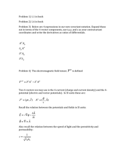


© Copyright 2026