
Numerical Algorithms - Stanford University
Justin Solomon
Numerical Algorithms
In memory of Clifford Nass
(1958–2013)
Contents
Section I Preliminaries
Chapter 1 Mathematics Review
1.1
1.2
1.3
1.4
1.5
PRELIMINARIES: NUMBERS AND SETS
VECTOR SPACES
1.2.1 Defining Vector Spaces
1.2.2 Span, Linear Independence, and Bases
1.2.3 Our Focus: Rn
LINEARITY
1.3.1 Matrices
1.3.2 Scalars, Vectors, and Matrices
1.3.3 Matrix Storage and Multiplication Methods
1.3.4 Model Problem: A~x = ~b
NON-LINEARITY: DIFFERENTIAL CALCULUS
1.4.1 Differentiation in One Variable
1.4.2 Differentiation in Multiple Variables
1.4.3 Optimization
EXERCISES
Chapter 2 Numerics and Error Analysis
2.1
2.2
2.3
2.4
STORING NUMBERS WITH FRACTIONAL PARTS
2.1.1 Fixed-Point Representations
2.1.2 Floating-Point Representations
2.1.3 More Exotic Options
UNDERSTANDING ERROR
2.2.1 Classifying Error
2.2.2 Conditioning, Stability, and Accuracy
PRACTICAL ASPECTS
2.3.1 Computing Vector Norms
2.3.2 Larger-Scale Example: Summation
EXERCISES
3
3
4
4
5
7
9
10
12
13
15
16
16
17
20
23
27
27
28
29
31
32
33
35
36
37
37
39
vii
viii Contents
Section II Linear Algebra
Chapter 3 Linear Systems and the LU Decomposition
3.1
3.2
3.3
47
SOLVABILITY OF LINEAR SYSTEMS
AD-HOC SOLUTION STRATEGIES
ENCODING ROW OPERATIONS
3.3.1 Permutation
3.3.2 Row Scaling
3.3.3 Elimination
GAUSSIAN ELIMINATION
3.4.1 Forward-Substitution
3.4.2 Back-Substitution
3.4.3 Analysis of Gaussian Elimination
LU FACTORIZATION
3.5.1 Constructing the Factorization
3.5.2 Using the Factorization
3.5.3 Implementing LU
EXERCISES
47
49
51
51
52
52
55
55
56
57
58
59
60
61
62
Chapter 4 Designing and Analyzing Linear Systems
65
3.4
3.5
3.6
4.1
4.2
4.3
4.4
SOLUTION OF SQUARE SYSTEMS
4.1.1 Regression
4.1.2 Least-Squares
4.1.3 Tikhonov Regularization
4.1.4 Image Alignment
4.1.5 Deconvolution
4.1.6 Harmonic Parameterization
SPECIAL PROPERTIES OF LINEAR SYSTEMS
4.2.1 Positive Definite Matrices and the Cholesky Factorization
4.2.2 Sparsity
4.2.3 Additional Special Structures
SENSITIVITY ANALYSIS
4.3.1 Matrix and Vector Norms
4.3.2 Condition Numbers
EXERCISES
Chapter 5 Column Spaces and QR
5.1
5.2
THE STRUCTURE OF THE NORMAL EQUATIONS
ORTHOGONALITY
65
66
68
70
71
73
74
75
75
79
81
81
82
84
87
93
93
94
Contents ix
5.3
5.4
5.5
5.6
5.7
STRATEGY FOR NON-ORTHOGONAL MATRICES
GRAM-SCHMIDT ORTHOGONALIZATION
5.4.1 Projections
5.4.2 Gram-Schmidt Algorithm
HOUSEHOLDER TRANSFORMATIONS
REDUCED QR FACTORIZATION
EXERCISES
Chapter 6 Eigenvectors
6.1
6.2
6.3
6.4
6.5
6.6
MOTIVATION
6.1.1 Statistics
6.1.2 Differential Equations
6.1.3 Spectral Embedding
PROPERTIES OF EIGENVECTORS
6.2.1 Symmetric and Positive Definite Matrices
6.2.2 Specialized Properties
6.2.2.1 Characteristic Polynomial
6.2.2.2 Jordan Normal Form
COMPUTING A SINGLE EIGENVALUE
6.3.1 Power Iteration
6.3.2 Inverse Iteration
6.3.3 Shifting
FINDING MULTIPLE EIGENVALUES
6.4.1 Deflation
6.4.2 QR Iteration
6.4.3 Krylov Subspace Methods
SENSITIVITY AND CONDITIONING
EXERCISES
Chapter 7 Singular Value Decomposition
7.1
7.2
DERIVING THE SVD
7.1.1 Computing the SVD
APPLICATIONS OF THE SVD
7.2.1 Solving Linear Systems and the Pseudoinverse
7.2.2 Decomposition into Outer Products and Low-Rank Approximations
7.2.3 Matrix Norms
7.2.4 The Procrustes Problem and Point Cloud Alignment
7.2.5 Principal Component Analysis (PCA)
95
96
96
98
101
105
106
109
109
110
111
112
114
116
118
118
119
119
119
121
121
122
123
124
128
129
130
135
135
137
138
138
139
140
141
143
x Contents
7.3
7.2.6 Eigenfaces
EXERCISES
143
145
Section III Nonlinear Techniques
Chapter 8 Nonlinear Systems
8.1
8.2
8.3
8.4
ROOT-FINDING IN A SINGLE VARIABLE
8.1.1 Characterizing Problems
8.1.2 Continuity and Bisection
8.1.3 Fixed Point Iteration
8.1.4 Newton’s Method
8.1.5 Secant Method
8.1.6 Hybrid Techniques
8.1.7 Single-Variable Case: Summary
MULTIVARIABLE PROBLEMS
8.2.1 Newton’s Method
8.2.2 Making Newton Faster: Quasi-Newton and Broyden
CONDITIONING
EXERCISES
Chapter 9 Unconstrained Optimization
9.1
9.2
9.3
9.4
9.5
9.6
UNCONSTRAINED OPTIMIZATION: MOTIVATION
OPTIMALITY
9.2.1 Differential Optimality
9.2.2 Alternative Conditions for Optimality
ONE-DIMENSIONAL STRATEGIES
9.3.1 Newton’s Method
9.3.2 Golden Section Search
MULTIVARIABLE STRATEGIES
9.4.1 Gradient Descent
9.4.2 Newton’s Method in Multiple Variables
9.4.3 Optimization without Hessians: BFGS
EXERCISES
APPENDIX: DERIVATION OF BFGS UPDATE
Chapter 10 Constrained Optimization
10.1
10.2
MOTIVATION
THEORY OF CONSTRAINED OPTIMIZATION
10.2.1 Optimality
151
151
151
152
153
155
157
159
159
160
160
161
162
163
167
167
169
170
172
174
174
174
176
176
179
179
182
186
189
190
193
193
Contents xi
10.2.2 KKT Conditions
OPTIMIZATION ALGORITHMS
10.3.1 Sequential Quadratic Programming (SQP)
10.3.1.1 Equality constraints
10.3.1.2 Inequality Constraints
10.3.2 Barrier Methods
10.4 CONVEX PROGRAMMING
10.4.1 Linear Programming
10.4.2 Second-Order Cone Programming
10.4.3 Semidefinite Programming
10.4.4 Integer Programs and Relaxations
10.5 EXERCISES
10.3
Chapter 11 Iterative Linear Solvers
11.1
11.2
11.3
11.4
11.5
GRADIENT DESCENT
11.1.1 Gradient Descent for Linear Systems
11.1.2 Convergence
CONJUGATE GRADIENTS
11.2.1 Motivation
11.2.2 Suboptimality of Gradient Descent
11.2.3 Generating A-Conjugate Directions
11.2.4 Formulating the Conjugate Gradients Algorithm
11.2.5 Convergence and Stopping Conditions
PRECONDITIONING
11.3.1 CG with Preconditioning
11.3.2 Common Preconditioners
OTHER ITERATIVE ALGORITHMS
EXERCISES
Chapter 12 Specialized Optimization Methods
12.1
NONLINEAR LEAST SQUARES
12.1.1 Gauss-Newton
12.1.2 Levenberg-Marquardt
12.2 ITERATIVELY-REWEIGHTED LEAST SQUARES
12.3 COORDINATE DESCENT AND ALTERNATION
12.3.1 Identifying Candidates for Alternation
12.3.2 Augmented Lagrangians and ADMM
12.4 GLOBAL OPTIMIZATION
12.4.1 Graduated Optimization
193
196
197
197
197
198
198
200
201
203
204
205
211
212
212
213
215
216
217
219
220
223
223
224
225
226
227
231
231
232
233
234
235
235
239
244
245
xii Contents
12.5
12.6
12.4.2 Randomized Global Optimization
ONLINE OPTIMIZATION
EXERCISES
247
249
252
Section IV Functions, Derivatives, and Integrals
Chapter 13 Interpolation
13.1
INTERPOLATION IN A SINGLE VARIABLE
13.1.1 Polynomial Interpolation
13.1.2 Alternative Bases
13.1.3 Piecewise Interpolation
13.2 MULTIVARIABLE INTERPOLATION
13.2.1 Nearest-Neighbor Interpolation
13.2.2 Barycentric Interpolation
13.2.3 Grid-Based Interpolation
13.3 THEORY OF INTERPOLATION
13.3.1 Linear Algebra of Functions
13.3.2 Approximation via Piecewise Polynomials
13.4 EXERCISES
Chapter 14 Integration and Differentiation
14.1
14.2
MOTIVATION
QUADRATURE
14.2.1 Interpolatory Quadrature
14.2.2 Quadrature Rules
14.2.3 Newton-Cotes Quadrature
14.2.4 Gaussian Quadrature
14.2.5 Adaptive Quadrature
14.2.6 Multiple Variables
14.2.7 Conditioning
14.3 DIFFERENTIATION
14.3.1 Differentiating Basis Functions
14.3.2 Finite Differences
14.3.3 Richardson Extrapolation
14.3.4 Choosing the Step Size
14.3.5 Automatic Differentiation
14.3.6 Integrated Quantities and Structure Preservation
14.4 EXERCISES
Chapter 15 Ordinary Differential Equations
261
262
262
266
267
269
269
270
272
273
273
276
277
283
284
285
286
287
288
292
293
295
296
297
297
298
299
300
301
302
304
309
Contents xiii
15.1
15.2
15.3
15.4
15.5
15.6
MOTIVATION
THEORY OF ODES
15.2.1 Basic Notions
15.2.2 Existence and Uniqueness
15.2.3 Model Equations
TIME-STEPPING SCHEMES
15.3.1 Forward Euler
15.3.2 Backward Euler
15.3.3 Trapezoidal Method
15.3.4 Runge-Kutta Methods
15.3.5 Exponential Integrators
MULTIVALUE METHODS
15.4.1 Newmark Integrators
15.4.2 Staggered Grid and Leapfrog
COMPARISON OF INTEGRATORS
EXERCISES
Chapter 16 Partial Differential Equations
16.1
16.2
16.3
16.4
16.5
16.6
16.7
MOTIVATION
STATEMENT AND STRUCTURE OF PDES
16.2.1 Properties of PDEs
16.2.2 Boundary Conditions
MODEL EQUATIONS
16.3.1 Elliptic PDEs
16.3.2 Parabolic PDEs
16.3.3 Hyperbolic PDEs
REPRESENTING DERIVATIVE OPERATORS
16.4.1 Finite Differences
16.4.2 Collocation
16.4.3 Finite Elements
16.4.4 Finite Volumes
16.4.5 Other Methods
SOLVING PARABOLIC AND HYPERBOLIC EQUATIONS
16.5.1 Semidiscrete Methods
16.5.2 Fully Discrete Methods
NUMERICAL CONSIDERATIONS
16.6.1 Consistency, Convergence, and Stability
16.6.2 Linear Solvers for PDE
EXERCISES
310
311
311
313
315
317
317
319
320
321
323
324
325
327
329
330
335
336
341
341
342
344
344
345
346
347
348
352
353
356
357
358
358
359
360
360
361
361
Preface
OMPUTER science is experiencing a fundamental shift in its approach to modeling
and problem solving. Early computer scientists primarily studied discrete mathematics,
focusing on structures like graphs, trees, and arrays composed of a finite number of distinct
pieces. With the introduction of fast floating-point processing alongside “big data,” threedimensional scanning, and other sources of noisy input, modern practitioners of computer
science must design robust methods for processing and understanding real-valued data. Now,
alongside discrete mathematics computer scientists must be equally fluent in the languages
of multivariable calculus and linear algebra.
Numerical Algorithms introduces the skills necessary to be both clients and designers
of numerical methods for computer science applications. This text is designed for advanced
undergraduate and early graduate students who are comfortable with mathematical notation and formality but need to review continuous concepts alongside the algorithms under
consideration. It covers a broad base of topics, from numerical linear algebra to optimization
and differential equations, with the goal of deriving standard approaches while developing
the intuition and comfort needed to understand more extensive literature in each subtopic.
Thus, each chapter gently but rigorously introduces numerical methods alongside mathematical background and motivating examples from modern computer science.
Nearly every section considers real-world use cases for a given class of numerical algorithms. For example, the singular value decomposition is introduced alongside statistical
methods, point cloud alignment, and low-rank approximation, and the discussion of leastsquares includes concepts from machine learning like kernelization and regularization. The
goal of this presentation of theory and application in parallel is to improve intuition for the
design of numerical methods and the application of each method to practical situations.
Special care has been taken to provide unifying threads from chapter to chapter. This
strategy helps relate discussions of seemingly independent problems, reinforcing skills while
presenting increasingly complex algorithms. In particular, starting with a chapter on mathematical preliminaries, methods are introduced with variational principles in mind, e.g.,
solving the linear system A~x = ~b by minimizing the energy kA~x − ~bk22 or finding eigenvectors as critical points of the Rayleigh quotient.
The book is organized into sections covering a few large-scale topics:
C
I. Preliminaries covers themes that appear in all branches of numerical algorithms. We
start with a review of relevant notions from continuous mathematics, designed as a
refresher for students who have not made extensive use of calculus or linear algebra
since their introductory math classes. This chapter can be skipped if students are
confident in their mathematical abilities, but even advanced readers may consider
taking a look to understand notation and basic constructions that will be used repeatedly later on. Then, we proceed with a chapter on numerics and error analysis,
the basic tools of numerical analysis for representing real numbers and understanding
the quality of numerical algorithms. In many ways, this chapter explicitly covers the
high-level themes that make numerical algorithms different from discrete algorithms:
In this domain, we rarely expect to recover exact solutions to computational problems
but rather approximate them.
xv
xvi Preface
II. Linear Algebra covers the algorithms needed to solve and analyze linear systems of
equations. This section is designed not only to cover the algorithms found in any
treatment of numerical linear algebra—including Gaussian elimination, matrix factorization, and eigenvalue computation—but also to motivate why these tools are
useful for computer scientists. To this end, we will explore wide-ranging applications
in data analysis, image processing, and even face recognition, showing how each can be
reduced to an appropriate matrix problem. This discussion will reveal that numerical
linear algebra is far from an exercise in abstract algorithmics; rather, it is a tool that
can be applied to countless computational models.
III. Nonlinear Techniques explores the structure of problems that do not reduce to
linear systems of equations. Two key tasks arise in this section, root-finding and optimization, which are related by Lagrange multipliers and other optimality conditions.
Nearly any modern algorithm for machine learning involves optimization of some objective, so we will find no shortage of examples from recent research and engineering.
After developing basic iterative methods for constrained and unconstrained optimization, we will return to the linear system A~x = ~b, developing the conjugate gradients
algorithm for approximating ~x using optimization tools. We conclude this section with
a discussion of “specialized” optimization algorithms, which are gaining popularity in
recent research. This chapter, whose content does not appear in classical texts, covers
strategies for developing algorithms specifically to minimize a single energy functional.
This approach contrasts with our earlier treatment of generic approaches for minimization that work for broad classes of objectives, presenting computational challenges on
paper with the reward of increased optimization efficiency.
IV. Functions, Derivatives, and Integrals concludes our consideration of numerical
algorithms by examining problems in which an entire function rather than a single value or point is the unknown. Example tasks in this class include interpolation,
approximation of derivatives and integrals of a function from samples, and solution of
differential equations. In addition to classical applications in computational physics,
we will show how these tools are relevant to a wide range of problems including rendering of three-dimensional shapes, x-ray scanning, and geometry processing.
Individual chapters are designed to be fairly independent, but of course it is impossible
to orthogonalize the content completely. For example, iterative methods for optimization
and root-finding must solve linear systems of equations in each iteration, and some interpolation methods can be posed as optimization problems. In general, Parts III (Nonlinear
Techniques) and IV (Functions, Derivatives, and Integrals) are largely independent of one
another but both depend on matrix algorithms developed in Part II (Linear Algebra). In
each part, the chapters are presented in order of importance. Initial chapters introduce key
themes in the subfield of numerical algorithms under consideration, while later chapters
focus on advanced algorithms adjacent to new research; sections within each chapter are
organized in a similar fashion.
Numerical algorithms are very different from algorithms approached in most other
branches of computer science, and students should expect to be challenged the first time
they study this material. With practice, however, it can be easy to build up intuition for
this unique and widely applicable field. To support this goal, each chapter concludes with
a set of problems designed to encourage critical thinking about the material at hand.
Simple computational problems in large part are omitted from the text, under the expectation that active readers approach the book with pen and paper in hand. Some suggestions
of exercises that can help readers as they peruse the material, but are not explicitly included
in the end-of-chapter problems, include the following:
Preface xvii
1. Try each algorithm by hand. For instance, after reading the discussion of algorithms
for solving the linear system A~x = ~b, write down a small matrix A and corresponding
vector ~b, and make sure you can recover ~x by following the steps the algorithm. After
reading the treatment of optimization, write down a specific function f (~x) and a
few iterates ~x1 , ~x2 , ~x3 , . . . of an optimization method to make sure f (~x1 ) ≥ f (~x2 ) ≥
f (~x3 ) > · · · .
2. Implement the algorithms in software and experiment with their behavior. Many numerical algorithms take on beautifully succinct—and completely abstruse—forms that
must be unraveled when they are implemented in code. Plus, nothing is more rewarding than the moment when a piece of numerical code begins functioning properly,
transitioning from an abstract sequence of mathematical statements to a piece of
machinery systematically solving equations or decreasing optimization objectives.
3. Attempt to derive algorithms by hand without referring to the discussion in the book.
The best way to become an expert in numerical analysis is to be able to reconstruct
the basic algorithms by hand, an exercise that supports intuition for the existing
methods and will help suggest extensions to other problems you may encounter.
Any large-scale treatment of a field as diverse and classical as numerical algorithms is
bound to omit certain topics, and inevitably decisions of this nature may be controversial to
readers with different backgrounds. This book is designed for a one- to two-semester course
in numerical algorithms, for computer scientists rather than mathematicians or engineers in
scientific computing. This target audience has led to a focus on modeling and applications
rather than on general proofs of convergence, error bounds, and the like; the discussion
includes references to more specialized or advanced literature when possible. Some topics,
including the fast Fourier transform, algorithms for sparse linear systems, Monte Carlo
methods, adaptivity in solving differential equations, and multigrid methods, are mentioned
only in passing or in exercises in favor of explaining modern developments in optimization
and other algorithms that have gained recent popularity. Future editions of this textbook
may incorporate these or other topics depending on feedback from instructors and readers.
The refinement of course notes and other materials leading to this textbook benefited
from the generous input of my students and colleagues. In the interests of maintaining these
materials and responding to the needs of students and instructors, please do not hesitate
to contact me with questions, comments, concerns, or ideas for potential changes.
Justin Solomon
Acknowledgments
REPARATION of this textbook would not have been possible without the support
of countless individuals and organizations. I have attempted to acknowledge some of
the many contributors and supporters below. I cannot thank these colleagues and friends
enough for their patience and attention throughout this undertaking.
The book is dedicated to the memory of Professor Clifford Nass, whose guidance fundamentally shaped my early academic career. His wisdom, teaching, encouragement, enthusiasm, and unique sense of style all will be missed on the Stanford campus and in the larger
community.
My mother, Nancy Griesemer, was the first to suggest expanding my teaching materials
into a text. I would not have been able to find the time or energy to prepare this work
without her support or that from my father Rod Solomon; my sister Julia Solomon Ensor,
her husband Jeff Ensor, and their daughter Caroline Ensor; and my grandmothers Juddy
Solomon and Dolores Griesemer. My uncle Peter Silberman and aunt Dena Silberman have
supported my academic career from its inception. Many other family members also should
be thanked including Archa and Joseph Emerson; Jerry, Jinny, Kate, Bonnie, and Jeremiah
Griesemer; Jim, Marge, Paul, Laura, Jarrett, Liza, Jiana, Lana, Jahson, Jaime, Gabriel, and
Jesse Solomon; Chuck and Louise Silverberg; and Barbara, Kerry, Greg, and Amy Schaner.
My career at Stanford has been guided primarily by my advisor Leonidas Guibas and
co-advisor Adrian Butscher. The approaches I take to many of the problems in the book
undoubtedly imitate the problem-solving strategies they have taught me. Ron Fedkiw suggested I teach the course leading to this text and provided advice on preparing the material.
My collaborators in the Geometric Computing Group and elsewhere on campus—including
Roland Angst, Mirela Ben-Chen, Tanya Glozman, Jonathan Huang, Qixing Huang, Michael
Kerber, Andy Nguyen, Maks Ovsjanikov, Franco Pestilli, Chris Piech, Raif Rustamov, and
Fan Wang—kindly have allowed me to use some research time to complete this text and
have helped refine the discussion at many points. Staff in the Stanford computer science department, including Meredith Hutchin, Claire Stager, and Steven Magness, made it possible
to organize my numerical algorithms course and many others.
I owe many thanks to the students of Stanford’s CS 205A course (fall 2013) for catching
numerous typos and mistakes in an early draft of this book. The following is a no-doubt
incomplete list of students and course assistants who contributed to this effort: Scott Chung,
Tao Du, Lennart Jansson, Miles Johnson, David Hyde, Luke Knepper, Minjae Lee, Nisha
Masharani, David McLaren, Catherine Mullings, John Reyna, William Song, Ben-Han Sung,
Martina Troesch, Ozhan Turgut, Patrick Ward, Joongyeub Yeo, and Yang Zhao.
David Hyde and Scott Chung continued to provide detailed feedback in winter and spring
2014. In addition, they helped prepare figures and end-of-chapter problems. Problems that
they drafted are marked DH and SC, respectively.
I leaned upon several colleagues and friends to help edit the text. In addition to those
mentioned above, additional contributors include: Nick Alger, George Anderson, Rahil
Baber, Nicolas Bonneel, Chen Chen, Matthew Cong, Roy Frostig, Jessica Hwang, Howon
Lee, Julian Kates-Harbeck, Jonathan Lee, Niru Maheswaranathan, Mark Pauly, Dan Robinson, and Hao Zhuang.
P
xix
xx Acknowledgments
Special thanks to Jan Heiland and Tao Du for helping clarify the derivation of the BFGS
algorithm.
Charlotte Byrnes, Sarah Chow, Randi Cohen, Kate Gallo, and Hayley Ruggieri at Taylor
& Francis guided me through the publication process and answered countless questions as
I prepared this work for print.
The Hertz Foundation provided a valuable network of experienced and knowledgeable
members of the academic community. In particular, Louis Lerman provided career advice
throughout my PhD that shaped my approach to research and navigating academia. Other
members of the Hertz community who provided guidance include Diann Callaghan, Wendy
Cieslak, Jay Davis, Philip Eckhoff, Linda Kubiak, Amanda O’Connor, Linda Souza, Thomas
Weaver, and Katherine Young. I should also acknowledge the NSF GRFP and NDSEG
fellowships for their support.
A multitude of friends supported this work in assorted stages of its development. Additional collaborators and mentors in the research community who have discussed and encouraged this work include Keenan Crane, Michael Eichmair, Hao Li, Niloy Mitra, Helmut
Pottmann, Fei Sha, Olga Sorkine-Hornung, Amir Vaxman, Etienne Vouga, Brian Wandell,
and Chris Wojtan. The first several chapters of this book were drafted on tour with the
Stanford Symphony Orchestra on their European tour “In Beethoven’s Footsteps” (summer 2013). Beyond this tour, Geri Actor, Susan Bratman, Debra Fong, Stephen Harrison,
Patrick Kim, Mindy Perkins, Thomas Shoebotham, and Lowry Yankwich all supported musical breaks during the drafting of this book. Prometheus Athletics provided an unexpected
outlet, and I should thank Archie de Torres, Amy Giver, Lori Giver, Troy Obrero, and Ben
Priestley for allowing me to be an enthusiastic if clumsy participant.
Additional friends who have lent advice, assistance, and time to this effort include: Chris
Aakre, Katy Ashe, Katya Avagian, Kyle Barrett, Noelle Beegle, Gilbert Bernstein, Elizabeth
Blaber, Lia Bonamassa, Eric Boromisa, Karen Budd, Avery Bustamante, Rose Casey, Arun
Chaganty, Phil Chen, Andrew Chou, Bernie Chu, Cindy Chu, Victor Cruz, Elan Dagenais,
Abe Davis, Matthew Decker, Bailin Deng, Martin Duncan, Eric Ellenoff, James Estrella,
Alyson Falwell, Anna French, Adair Gerke, Christina Goeders, Gabrielle Gulo, Nathan
Hall-Snyder, Logan Hehn, Jo Jaffe, Dustin Janatpour, Brandon Johnson, Victoria Johnson, Jeff Gilbert, Stephanie Go, Alex Godofsky, Alan Guo, Randy Hernando, Petr Johanes,
Maria Judnick, Ken Kao, Jonathan Kass, Gavin Kho, Hyungbin Kim, Sarah Kongpachith,
Jim Lalonde, Lauren Lax, Atticus Lee, Eric Lee, Menyoung Lee, Letitia Lew, Siyang Li,
Adrian Lim, Yongwhan Lim, Alex Louie, Lily Louie, Cleo Messinger, Courtney Meyer,
Daniel Meyer, Lisa Newman, Logan Obrero, Pualani Obrero, Thomas Obrero, Molly Pam,
David Parker, Madeline Paymer, Cuauhtemoc Peranda, Fabianna Perez, Bharath Ramsundar, Arty Rivera, Daniel Rosenfeld, Te Rutherford, Ravi Sankar, Aaron Sarnoff, Amanda
Schloss, Keith Schwarz, Steve Sellers, Charlton Soesanto, Mark Smitt, Jacob Steinhardt,
Charlie Syms, Andrea Tagliasacchi, Michael Tamkin, Sumil Thapa, Herb Tyson, Katie
Tyson, Madeleine Udell, Greg Valdespino, Walter Vulej, Thomas Waggoner, Frank Wang,
Sydney Wang, Susanna Wen, Genevieve Williams, Molby Wong, Eddy Wu, Winston Yan,
and Evan Young.
I
Preliminaries
1
CHAPTER
1
Mathematics Review
CONTENTS
1.1
1.2
Preliminaries: Numbers and Sets . . . . . . . . . . . . . . . . . . . . . . . . . . . . . . . . . . . . . . .
Vector Spaces . . . . . . . . . . . . . . . . . . . . . . . . . . . . . . . . . . . . . . . . . . . . . . . . . . . . . . . . . . .
1.2.1 Defining Vector Spaces . . . . . . . . . . . . . . . . . . . . . . . . . . . . . . . . . . . . . . . . . .
1.2.2 Span, Linear Independence, and Bases . . . . . . . . . . . . . . . . . . . . . . . . .
1.2.3 Our Focus: Rn . . . . . . . . . . . . . . . . . . . . . . . . . . . . . . . . . . . . . . . . . . . . . . . . . .
Linearity . . . . . . . . . . . . . . . . . . . . . . . . . . . . . . . . . . . . . . . . . . . . . . . . . . . . . . . . . . . . . . . .
1.3.1 Matrices . . . . . . . . . . . . . . . . . . . . . . . . . . . . . . . . . . . . . . . . . . . . . . . . . . . . . . . . .
1.3.2 Scalars, Vectors, and Matrices . . . . . . . . . . . . . . . . . . . . . . . . . . . . . . . . . .
1.3.3 Matrix Storage and Multiplication Methods . . . . . . . . . . . . . . . . . . .
1.3.4 Model Problem: A~x = ~b . . . . . . . . . . . . . . . . . . . . . . . . . . . . . . . . . . . . . . . . .
Non-Linearity: Differential Calculus . . . . . . . . . . . . . . . . . . . . . . . . . . . . . . . . . . . .
1.4.1 Differentiation in One Variable . . . . . . . . . . . . . . . . . . . . . . . . . . . . . . . . .
1.4.2 Differentiation in Multiple Variables . . . . . . . . . . . . . . . . . . . . . . . . . . . .
1.4.3 Optimization . . . . . . . . . . . . . . . . . . . . . . . . . . . . . . . . . . . . . . . . . . . . . . . . . . . .
1.3
1.4
3
4
4
5
7
9
10
12
13
15
16
16
17
20
N this chapter, we will outline notions from linear algebra and multivariable calculus that
will be relevant to our discussion of computational techniques. It is intended as a review
of background material with a bias toward ideas and interpretations commonly encountered
in practice; the chapter can be safely skipped or used as reference by students with stronger
background in mathematics.
I
1.1
PRELIMINARIES: NUMBERS AND SETS
Rather than considering algebraic (and at times philosophical) discussions like “What is a
number?,” we will rely on intuition and mathematical common sense to define a few sets:
• The natural numbers N = {1, 2, 3, . . .}
• The integers Z = {. . . , −2, −1, 0, 1, 2, . . .}
• The rational numbers Q = {a/b : a, b ∈ Z, b 6= 0}
• The real numbers R encompassing Q as well as irrational numbers like π and
√
2
• The√complex numbers C = {a + bi : a, b ∈ R}, where we think of i as satisfying
i = −1.
The definition of Q is the first of many times that we will use the notation {A : B}; the
braces denote a set and the colon can be read as “such that.” For instance, the definition
of Q can be read as “the set of fractions a/b such that a and b are integers.” As a second
3
4 Numerical Algorithms
example, we could write N = {n ∈ Z : n > 0}. It is worth acknowledging that our definition
of R is far from rigorous. The construction of the real numbers can be an important topic
for practitioners of cryptography techniques that make use of alternative number systems,
but these intricacies are irrelevant for the discussion at hand.
As with any other sets, N, Z, Q, R, and C can be manipulated using generic operations
to generate new sets of numbers. In particular, we can define the “Euclidean product” of
two sets A and B as
A × B = {(a, b) : a ∈ A and b ∈ B}.
We can take powers of sets by writing
An = A × A × · · · × A .
´¹¹ ¹ ¹ ¹ ¹ ¹ ¹ ¹ ¹ ¹ ¹ ¹ ¹ ¹ ¹ ¹ ¹ ¹ ¹ ¹ ¹ ¹ ¸¹ ¹ ¹ ¹ ¹ ¹ ¹ ¹ ¹ ¹ ¹ ¹ ¹ ¹ ¹ ¹ ¹ ¹ ¹ ¹ ¹ ¹ ¹ ¶
n times
This construction yields what will become our favorite set of numbers in chapters to come:
Rn = {(a1 , a2 , . . . , an ) : ai ∈ R for all i}.
1.2
VECTOR SPACES
Introductory linear algebra courses easily could be titled “Introduction to FiniteDimensional Vector Spaces.” Although the definition of a vector space might appear abstract, we will find many concrete applications expressible in vector space language that
can benefit from the machinery we will develop.
1.2.1
Defining Vector Spaces
We begin by defining a vector space and providing a number of examples:
Definition 1.1 (Vector space over R). A vector space over R is a set V closed under
addition and scalar multiplication satisfying the following axioms:
• Additive commutativity and associativity: For all ~u, ~v , w
~ ∈ V, ~v + w
~ = w
~ + ~v and
(~u + ~v ) + w
~ = ~u + (~v + w).
~
• Distributivity: For all ~v , w
~ ∈ V and a, b ∈ R, a(~v + w)
~ = a~v +aw
~ and (a+b)~v = a~v +b~v .
• Additive identity: There exists ~0 ∈ V with ~0 + ~v = ~v for all ~v ∈ V.
• Additive inverse: For all ~v ∈ V, there exists w
~ ∈ V with ~v + w
~ = ~0.
• Multiplicative identity: For all ~v ∈ V, 1 · ~v = ~v .
• Multiplicative compatibility: For all ~v ∈ V and a, b ∈ R, (ab)~v = a(b~v ).
A member ~v ∈ V is known as a vector ; arrows will be used to indicate vector variables.
For our purposes, a scalar is a number in R; a complex vector space satisfies the same
definition with R replaced by C. It is usually straightforward to spot vector spaces in the
wild, including the following examples:
Mathematics Review 5
~v3
~v2
~v1
R2
(a) ~v1 , ~v2 ∈ R2
span {~v1 , ~v2 }
(b) span {~v1 , ~v2 }
(c) span {~v1 , ~v2 , ~v3 }
(a) Two vectors ~v1 , ~v2 ∈ R2 ; (b) their span is the whole plane R2 ; (c)
span {~v1 , ~v2 , ~v3 } = span {~v1 , ~v2 } because ~v3 can be written as a linear combination
of ~v1 and ~v2 .
Figure 1.1
Example 1.1 (Rn as a vector space). The most common example of a vector space is Rn .
Here, addition and scalar multiplication happen component-by-component:
(1, 2) + (−3, 4) = (1 − 3, 2 + 4) = (−2, 6)
10 · (−1, 1) = (10 · −1, 10 · 1) = (−10, 10).
Example 1.2 (Polynomials). A second example of a vector space is the ring of polynomials
with real-valued coefficients, denoted R[x]. A polynomial p ∈ R[x] is a function p : R → R
taking the form∗
X
p(x) =
ak xk .
k
Addition and scalar multiplication are carried out in the usual way, e.g., if p(x) = x2 +2x−1
and q(x) = x3 , then 3p(x) + 5q(x) = 5x3 + 3x2 + 6x − 3, which is another polynomial. As
an aside, for future examples note that functions like p(x) = (x − 1)(x + 1) + x2 (x3 − 5)
are still polynomials even though they are not explicitly written in the form above.
P
A weighted sum of the form
vi , where ai ∈ R and ~vi ∈ V, is known as a linear
i ai~
combination of the ~vi ’s. In the second example, the “vectors” are polynomials, although we
do not normally use this language to discuss R[x]; unless otherwise noted, we will assume
variables notated with arrows ~v are members ofP
Rn for some n. One way to link these two
viewpoints would be to identify the polynomial k ak xk with the sequence (a0 , a1 , a2 , . . .);
polynomials have finite numbers of terms, so this sequence eventually will end in a string
of zeros.
1.2.2
Span, Linear Independence, and Bases
Suppose we start with vectors ~v1 , . . . , ~vk ∈ V in vector space V. By Definition 1.1, we have
two ways to start with these vectors and construct new elements of V: addition and scalar
multiplication. The idea of span is that it describes all of the vectors you can reach via
these two operations:
∗ The notation f : A → B means f is a function that takes as input an element of set A and outputs an
element of set B. For instance, f : R → Z takes as input a real number in R and outputs an integer Z, as
might be the case for f (x) = bxc, the “round down” function.
6 Numerical Algorithms
Definition 1.2 (Span). The span of a set S ⊆ V of vectors is the set
span S ≡ {a1~v1 + · · · + ak~vk : ~vi ∈ V and ai ∈ R for all i}.
Figure 1.1(b) illustrates the span of two vectors shown in Figure 1.1(a). By definition, span S
is a subspace of V, that is, a subset of V that is itself a vector space. We can provide a few
examples:
Example 1.3 (Mixology). The typical well at a cocktail bar contains at least four ingredients at the bartender’s disposal: vodka, tequila, orange juice, and grenadine. Assuming
we have this well, we can represent drinks as points in R4 , with one element for each ingredient. For instance, a tequila sunrise can be represented using the point (0, 1.5, 6, 0.75),
representing amounts of vodka, tequila, orange juice, and grenadine (in ounces), respectively.
The set of drinks that can be made with our well is contained in
span {(1, 0, 0, 0), (0, 1, 0, 0), (0, 0, 1, 0), (0, 0, 0, 1)},
that is, all combinations of the four basic ingredients. A bartender looking to save time,
however, might notice that many drinks have the same orange juice-to-grenadine ratio
and mix the bottles. The new simplified well may be easier for pouring but can make
fundamentally fewer drinks:
span {(1, 0, 0, 0), (0, 1, 0, 0), (0, 0, 6, 0.75)}.
For example, this reduced well cannot fulfill orders for a screwdriver, which contains orange
juice but not grenadine.
Example 1.4 (Cubic polynomials). Define pk (x) ≡ xk . With this notation, the set of
cubic polynomials can be written in two equivalent ways
{ax3 + bx2 + cx + d ∈ R[x] : a, b, c, d ∈ R} = span {p0 , p1 , p2 , p3 }.
Adding another item to a set of vectors does not always increase the size of its span, as
illustrated in Figure 1.1(c). For instance, in R2 ,
span {(1, 0), (0, 1)} = span {(1, 0), (0, 1), (1, 1)}.
In this case, we say that the set {(1, 0), (0, 1), (1, 1)} is linearly dependent:
Definition 1.3 (Linear dependence). We provide three equivalent definitions. A set S ⊆ V
of vectors is linearly dependent if:
1. One of the elements of S can be written as a linear combination of the other elements,
or S contains zero.
2. P
There exists a non-empty linear combination of elements ~vk ∈ S yielding
m
vk = 0 where ck 6= 0 for all k.
k=1 ck ~
3. There exists ~v ∈ S such that span S = span S\{~v }. That is, we can remove a vector
from S without affecting its span.
If S is not linearly dependent, then we say it is linearly independent.
Mathematics Review 7
Providing proof or informal evidence that each definition is equivalent to its counterparts
(in an “if and only if” fashion) is a worthwhile exercise for students less comfortable with
notation and abstract mathematics.
The concept of linear dependence provides an idea of “redundancy” in a set of vectors. In
this sense, it is natural to ask how large a set we can construct before adding another vector
cannot possibly increase the span. More specifically, suppose we have a linearly independent
set S ⊆ V, and now we choose an additional vector ~v ∈ V. Adding ~v to S has one of two
possible outcomes:
1. The span of S ∪ {~v } is larger than the span of S.
2. Adding ~v to S has no effect on its span.
The dimension of V counts the number of times we can get the first outcome while building
up a set of vectors:
Definition 1.4 (Dimension and basis). The dimension of V is the maximal size |S| of a
linearly independent set S ⊂ V such that span S = V. Any set S satisfying this property
is called a basis for V.
Example 1.5 (Rn ). The standard basis for Rn is the set of vectors of the form
~ek ≡ ( 0, . . . , 0, 1, 0, . . . , 0 ).
´¹¹ ¹ ¹ ¹ ¹ ¹ ¸¹ ¹ ¹ ¹ ¹ ¹ ¹¶
´¹¹ ¹ ¹ ¹ ¹ ¸ ¹ ¹ ¹ ¹ ¹ ¶
k−1 elements
n−k elements
That is, ~ek has all zeros except for a single one in the k-th position. These vectors are
linearly independent and form a basis for Rn ; for example in R3 any vector (a, b, c) can be
written as a~e1 + b~e2 + c~e3 . Thus, the dimension of Rn is n, as expected.
Example 1.6 (Polynomials). The set of monomials {1, x, x2 , x3 , . . .} is a linearly independent subset of R[x]. It is infinitely large, and thus the dimension of R[x] is ∞.
1.2.3
Our Focus: Rn
Of particular importance for our purposes is the vector space Rn , the so-called n-dimensional
Euclidean space. This is nothing more than the set of coordinate axes encountered in high
school math classes:
• R1 ≡ R is the number line.
• R2 is the two-dimensional plane with coordinates (x, y).
• R3 represents three-dimensional space with coordinates (x, y, z).
Nearly all methods in this book will deal with transformations of and functions on Rn .
For convenience, we usually write vectors in Rn in “column form,” as follows:
a1
a2
(a1 , . . . , an ) ≡ . .
..
an
8 Numerical Algorithms
This notation will include vectors as special cases of matrices discussed below.
Unlike some vector spaces, Rn has not only a vector space structure, but also one
additional construction that makes all the difference: the dot product.
Definition 1.5 (Dot product). The dot product of two vectors ~a = (a1 , . . . , an ) and
~b = (b1 , . . . , bn ) in Rn is given by
~a · ~b ≡
n
X
ak bk .
k=1
Example 1.7 (R2 ). The dot product of (1, 2) and (−2, 6) is 1 · −2 + 2 · 6 = −2 + 12 = 10.
The dot product is an example of a metric, and its existence gives a notion of geometry
to Rn . For instance, we can use the Pythagorean theorem to define the norm or length of
a vector ~a as the square root
q
√
k~ak2 ≡ a21 + · · · + a2n = ~a · ~a.
Then, the distance between two points ~a, ~b ∈ Rn is k~b − ~ak2 .
Dot products provide not only lengths and distances but also angles. The following
trigonometric identity holds for ~a, ~b ∈ R3 :
~a · ~b = k~ak2 k~bk2 cos θ,
where θ is the angle between ~a and ~b. When n ≥ 4, however, the notion of “angle” is much
harder to visualize in Rn . We might define the angle θ between ~a and ~b to be
θ ≡ arccos
~a · ~b
.
k~ak2 k~bk2
We must do our homework before making such a definition! In particular, cosine outputs
values in the interval [−1, 1], so we must check that the input to arc cosine (also notated
cos−1 ) is in this interval; thankfully, the well-known Cauchy-Schwarz inequality |~a · ~b| ≤
k~ak2 k~bk2 guarantees exactly this property.
When ~a = c~b for some c ∈ R, we have θ = arccos 1 = 0, as we would expect: The angle
between parallel vectors is zero. What does it mean for (nonzero) vectors to be perpendicular? Let’s substitute θ = 90◦ . Then, we have
0 = cos 90◦ =
~a · ~b
.
k~ak2 k~bk2
Multiplying both sides by k~ak2 k~bk2 motivates the definition:
Definition 1.6 (Orthogonality). Two vectors ~a, ~b ∈ Rn are perpendicular, or orthogonal,
when ~a · ~b = 0.
This definition is somewhat surprising from a geometric standpoint. We have managed to
define what it means to be perpendicular without any explicit use of angles.
Mathematics Review 9
Aside 1.1. There are many theoretical questions to ponder here, some of which we will
address in future chapters:
• Do all vector spaces admit dot products or similar structures?
• Do all finite-dimensional vector spaces admit dot products?
• What might be a reasonable dot product between elements of R[x]?
Intrigued students can consult texts on real and functional analysis.
1.3
LINEARITY
A function from one vector space to another that preserves linear structure is known as a
linear function:
Definition 1.7 (Linearity). Suppose V and V 0 are vector spaces. Then, L : V → V 0 is
linear if it satisfies the following two criteria for all ~v , ~v1 , ~v2 ∈ V and c ∈ R:
• L preserves sums: L[~v1 + ~v2 ] = L[~v1 ] + L[~v2 ]
• L preserves scalar products: L[c~v ] = cL[~v ]
It is easy to express linear maps between vector spaces, as we can see in the following
examples:
Example 1.8 (Linearity in Rn ). The following map f : R2 → R3 is linear:
f (x, y) = (3x, 2x + y, −y).
We can check linearity as follows:
• Sum preservation:
f (x1 + x2 , y1 + y2 ) = (3(x1 + x2 ), 2(x1 + x2 ) + (y1 + y2 ), −(y1 + y2 ))
= (3x1 , 2x1 + y1 , −y1 ) + (3x2 , 2x2 + y2 , −y2 )
= f (x1 , y1 ) + f (x2 , y2 )
• Scalar product preservation:
f (cx, cy) = (3cx, 2cx + cy, −cy)
= c(3x, 2x + y, −y)
= cf (x, y)
Contrastingly, g(x, y) ≡ xy 2 is not linear. For instance, g(1, 1) = 1, but g(2, 2) = 8 6=
2 · g(1, 1), so g does not preserve scalar products.
Example 1.9 (Integration). The following “functional” L from R[x] to R is linear:
Z
L[p(x)] ≡
1
p(x) dx.
0
10 Numerical Algorithms
This more abstract example maps polynomials p(x) ∈ R[x] to real numbers L[p(x)] ∈ R.
For example, we can write
Z 1
1
L[3x2 + x − 1] =
(3x2 + x − 1) dx = .
2
0
Linearity of L is a result of the following well-known identities from calculus:
Z 1
Z 1
f (x) dx
c · f (x) dx = c
0
Z
1
Z
0
1
0
0
Z
1
g(x) dx.
f (x) dx +
[f (x) + g(x)] dx =
0
We can write a particularly
nice form for linear maps on Rn . The vector ~a = (a1 , . . . , an )
P
is equal to the sum k ak~ek , where ~ek is the k-th standard basis vector from Example 1.5.
Then, if L is linear we can expand:
"
#
X
L[~a] = L
ak~ek for the standard basis ~ek
k
=
X
L [ak~ek ] by sum preservation
k
=
X
ak L [~ek ] by scalar product preservation.
k
This derivation shows:
A linear operator L on Rn is completely determined by its action
on the standard basis vectors ~ek .
That is, for any vector ~a ∈ Rn , we can use the sum above to determine L[~a] by linearly
combining L[~e1 ], . . . , L[~en ].
Example 1.10 (Expanding a linear map). Recall the map in Example 1.8 given by
f (x, y) = (3x, 2x + y, −y). We have f (~e1 ) = f (1, 0) = (3, 2, 0) and f (~e2 ) = f (0, 1) =
(0, 1, −1). Thus, the formula above shows:
3
0
f (x, y) = xf (~e1 ) + yf (~e2 ) = x 2 + y 1 .
−1
0
1.3.1
Matrices
The expansion of linear maps above suggests a context in which it is useful to store multiple
vectors in the same structure. More generally, say we have n vectors ~v1 , . . . , ~vn ∈ Rm . We
can write each as a column vector:
v11
v12
v1n
v21
v22
v2n
~v1 = . , ~v2 = . , · · · , ~vn = . .
..
..
..
vm1
vm2
vmn
Mathematics Review 11
Carrying these vectors around separately can be cumbersome
matters we combine them into a single m × n matrix:
v11 v12 · · ·
|
|
|
v21 v22 · · ·
~v1 ~v2 · · · ~vn = .
..
..
..
.
.
|
|
|
vm1 vm2 · · ·
notationally, so to simplify
v1n
v2n
..
.
.
vmn
We will call the space of such matrices Rm×n .
Example 1.11 (Identity matrix). We can store the standard
“identity matrix” In×n given by:
1 0 ···
0 1 ···
|
|
|
..
In×n ≡ ~e1 ~e2 · · · ~en = ... ...
.
|
|
|
0 0 ···
0 0 ···
basis for Rn in the n × n
0 0
0 0
.. .. .
. .
1 0
0 1
Since we constructed matrices as convenient ways to store sets of vectors, we can use
multiplication to express how they can be combined linearly. In particular, a matrix in
Rm×n can be multiplied by a column vector in Rn as follows:
c1
|
|
|
c2
~v1 ~v2 · · · ~vn
.. ≡ c1~v1 + c2~v2 + · · · + cn~vn .
.
|
|
|
cn
Expanding this sum yields
v11 v12 · · ·
v21 v22 · · ·
..
..
..
.
.
.
vm1 vm2 · · ·
the following explicit formula for matrix-vector products:
v1n
c1
c1 v11 + c2 v12 + · · · + cn v1n
v2n
c2 c1 v21 + c2 v22 + · · · + cn v2n
=
.
..
.
..
. ..
.
vmn
cn
c1 vm1 + c2 vm2 + · · · + cn vmn
Example 1.12 (Identity matrix multiplication). For any ~x ∈ Rn , we can write ~x = In×n ~x,
where In×n is the identity matrix from Example 1.11.
Example 1.13 (Linear map). We return once again to the function f (x, y) from Example 1.8 to show one more alternative form:
3 0
x
f (x, y) = 2 1
.
y
0 −1
We similarly define a product between a matrix M ∈ Rm×n and another matrix in Rn×p
with columns ~ci by concatenating individual matrix-vector products:
|
|
|
|
|
|
M ~c1 ~c2 · · · ~cn ≡ M~c1 M~c2 · · · M~cn .
|
|
|
|
|
|
12 Numerical Algorithms
Example 1.14 (Mixology). Continuing Example 1.3, suppose we make a tequila sunrise
and second concoction with equal parts of the two liquors in our simplified well. To find
out how much of the basic ingredients are contained in each order, we could combine the
recipes for each column-wise and use matrix multiplication:
Vodka
Tequila
OJ
Grenadine
Well 1
1
0
0
0
Well 2
0
1
0
0
Well 3
Drink 1
0
0
0
1.5
6
1
0.75
Drink 2
!
0.75
0.75
=
2
Drink 1
0
1.5
6
0.75
Drink
0.75
0.75
12
1.5
2
Vodka
Tequila
OJ
Grenadine
We will use capital letters to represent matrices, like A ∈ Rm×n . We will use the notation
Aij ∈ R to denote the element of A at row i and column j.
1.3.2
Scalars, Vectors, and Matrices
If we wish to unify notation completely, we can write a scalar as a 1 × 1 vector c ∈ R1×1 .
Similarly, as suggested in §1.2.3, if we write vectors in Rn in column form, they can be
considered n × 1 matrices ~v ∈ Rn×1 . Matrix-vector products also can be interpreted in this
context. For example, if A ∈ Rm×n , ~x ∈ Rn , and ~b ∈ Rm , then we can write expressions like
A · ~x = ~b .
® ®
®
m×n n×1
m×1
We will introduce one additional operator on matrices that is useful in this context:
Definition 1.8 (Transpose). The transpose of a matrix A ∈ Rm×n is a matrix A> ∈ Rn×m
with elements (A> )ij = Aji .
Example 1.15 (Transposition). The transpose of the matrix
1 2
A= 3 4
5 6
is given by
>
A =
1
2
3
4
5
6
.
Geometrically, we can think of transposition as flipping a matrix over its diagonal.
This unified treatment of scalars, vectors, and matrices combined with operations like
transposition and multiplication yields slick expressions and derivations of well-known identities. For instance, we can compute the dot products of vectors ~a, ~b ∈ Rn via the following
sequence of equalities:
b1
n
X
b2
~a · ~b =
ak bk = a1 a2 · · · an . = ~a>~b.
..
k=1
bn
Many identities from linear algebra can be derived by chaining together these operations
Mathematics Review 13
function Multiply(A, ~x)
. Returns ~b = A~x, where
. A ∈ Rm×n and ~x ∈ Rn
~b ← ~0
for i ← 1, 2, . . . , m
for j ← 1, 2, . . . , n
bi ← bi + aij xj
return ~b
(a)
Figure 1.2
function Multiply(A, ~x)
. Returns ~b = A~x, where
. A ∈ Rm×n and ~x ∈ Rn
~b ← ~0
for j ← 1, 2, . . . , n
for i ← 1, 2, . . . , m
bi ← bi + aij xj
return ~b
(b)
Two implementations of matrix-vector multiplication with different loop
ordering.
with a few rules:
(A> )> = A,
(A + B)> = A> + B > ,
(AB)> = B > A> .
and
Example 1.16 (Residual norm). Suppose we have a matrix A and two vectors ~x and ~b.
If we wish to know how well A~x approximates ~b, we might define a residual ~r ≡ ~b − A~x;
this residual is zero exactly when A~x = ~b. Otherwise, we can use the norm k~rk2 as a proxy
for the similarity of A~x and ~b. We can use the identities above to simplify:
k~rk22 = k~b − A~xk22
= (~b − A~x) · (~b − A~x) as explained in §1.2.3
= (~b − A~x)> (~b − A~x) by our expression for the dot product above
= (~b> − ~x> A> )(~b − A~x) by properties of transposition
= ~b>~b − ~b> A~x − ~x> A>~b + ~x> A> A~x after multiplication
All four terms on the right-hand side are scalars, or equivalently 1 × 1 matrices. Scalars
thought of as matrices enjoy one additional nice property c> = c, since there is nothing
to transpose! Thus,
~x> A>~b = (~x> A>~b)> = ~b> A~x.
This allows us to simplify even more:
k~rk22 = ~b>~b − 2~b> A~x + ~x> A> A~x
= kA~xk2 − 2~b> A~x + k~bk2 .
2
2
We could have derived this expression using dot product identities, but the intermediate
steps above will prove useful in later discussion.
1.3.3
Matrix Storage and Multiplication Methods
In this section, we take a brief detour from mathematical theory to consider practical
aspects of implementing linear algebra operations in computer software. Our discussion
considers not only faithfulness to the theory we have constructed but also the speed with
14 Numerical Algorithms
1 2
A= 3 4
5 6
(a)
1 2 3 4 5 6
(b) Row-major
1 3 5 2 4 6
(c) Column-major
Two possible ways to store (a) a matrix in memory: (b) row-major ordering
and (c) column-major ordering.
Figure 1.3
which we can carry out each operation. This is one of relatively few points at which we
will consider computer architecture and other engineering aspects of how computers are
designed. This consideration is necessary given the sheer number of times typical numerical
algorithms call down to linear algebra routines; a seemingly small improvement in implementing matrix-vector or matrix-matrix multiplication has the potential to increase the
efficiency of numerical routines by a large factor.
Figure 1.2 shows two possible implementations of matrix-vector multiplication. The
difference between these two algorithms is subtle and seemingly unimportant: The order of
the two loops has been switched. Rounding error aside, these two methods generate the same
output and do the same number of arithmetic operations; classical “big-O” analysis from
computer science would find these two methods indistinguishable. Surprisingly, however,
considerations related to computer architecture can make one of these options much faster
than the other!
A reasonable model for the memory or RAM in a computer is as a long line of data. For
this reason, we must find ways to “unroll” data from matrix form to something that could
be written completely horizontally. Two common patterns are illustrated in Figure 1.3:
• A row-major ordering stores the data row-by-row; that is, the first row appears in a
contiguous block of memory, then the second, and so on.
• A column-major ordering stores the data column-by-column, moving vertically first
rather than horizontally.
Consider the matrix multiplication method in Figure 1.2(a). This algorithm computes
all of b1 before moving to b2 , b3 , and so on. In doing so, the code moves along the elements
of A row-by-row. If A is stored in row-major order, then the algorithm in Figure 1.2(a)
proceeds linearly across its representation in memory (Figure 1.3(b)), whereas if A is stored
in column-major order (Figure 1.3(c)), the algorithm effectively jumps around between
elements in A. The opposite is true for the algorithm in Figure 1.2(b), which moves linearly
through the column-major ordering.
In many hardware implementations, loading data from memory will retrieve not just
the single requested value but instead a block of data near the request. The philosophy
here is that common algorithms move linearly though data, processing it one element at a
time, and anticipating future requests can reduce the communication load between the main
processor and the RAM. By pairing e.g., the algorithm in Figure 1.2(a) with the row-major
ordering in Figure 1.3(b), we can take advantage of this optimization by moving linearly
through the storage of the matrix A; the extra loaded data anticipates what will be needed
in the next iteration. If we take a nonlinear traversal through A in memory, this situation
is less likely, leading to a significant loss in speed.
Mathematics Review 15
1.3.4
Model Problem: A~x = ~b
In introductory algebra class, students spend considerable time solving linear systems such
as the following for triplets (x, y, z):
3x + 2y + 5z = 0
−4x + 9y − 3z = −7
2x − 3y − 3z = 1.
Our constructions in §1.3.1 allows us to encode
3
2
5
−4 9 −3
2 −3 −3
such systems in a cleaner fashion:
x
0
y = −7 .
z
1
More generally, we can write any linear system of equations in the form A~x = ~b by following the same pattern above; here, the vector ~x is unknown while A and ~b are known.
Such a system of equations is not always guaranteed to have a solution. For instance, if A
contains only zeros, then no ~x will satisfy A~x = ~b whenever ~b 6= ~0. We will defer a general
consideration of when a solution exists to our discussion of linear solvers in future chapters.
A key interpretation of the system A~x = ~b is that it addresses the task:
Write ~b as a linear combination of the columns of A.
Why? Recall from §1.3.1 that the product A~x encodes a linear combination of the columns
of A with weights contained in elements of ~x. So, the equation A~x = ~b sets the linear
combination A~x equal to the given vector ~b. Given this interpretation, we define the column
space of A to be the space of right-hand sides ~b for which the system A~x = ~b has a solution:
Definition 1.9 (Column space and rank). The column space of a matrix A ∈ Rm×n is
the span of the columns of A. It can be written as
col A ≡ {A~x : ~x ∈ Rn }.
The rank of A is the dimension of col A.
A~x = ~b is solvable exactly when ~b ∈ col A.
One case will dominate our discussion in future chapters. Suppose A is square, so we
can write A ∈ Rn×n . Furthermore, suppose that the system A~x = ~b has a solution for all
choices of ~b, so by our interpretation above the columns of A must span Rn . In this case,
we can substitute the standard basis ~e1 , . . . , ~en to solve equations of the form A~xi = ~ei ,
yielding vectors ~x1 , . . . , ~xn . Combining these ~xi ’s horizontally into a matrix shows:
|
|
|
|
|
|
A ~x1 ~x2 · · · ~xn = A~x1 A~x2 · · · A~xn
|
|
|
|
|
|
|
|
|
= ~e1 ~e2 · · · ~en = In×n ,
|
|
|
where In×n is the identity matrix from Example 1.11. We will call the matrix with columns
~xk the inverse A−1 , which satisfies
AA−1 = A−1 A = In×n .
16 Numerical Algorithms
15
10
5
0
f (x)
100
50
0
−50
−4−2 0 2 4
x
Figure 1.4
10
5
0
−2 −1 0
x
1
2
−1−0.5 0 0.5 1
x
The closer we zoom into f (x) = x3 + x2 − 8x + 4, the more it looks like a
line.
By construction, (A−1 )−1 = A. If we can find such an inverse, solving any linear system
A~x = ~b reduces to matrix multiplication, since:
~x = In×n ~x = (A−1 A)~x = A−1 (A~x) = A−1~b.
1.4
NON-LINEARITY: DIFFERENTIAL CALCULUS
While the beauty and applicability of linear algebra makes it a key target for study, nonlinearities abound in nature, and hence we must design machinery that can deal with this
reality.
1.4.1
Differentiation in One Variable
While many functions are globally nonlinear, locally they exhibit linear behavior. This idea
of “local linearity” is one of the main motivators behind differential calculus. Figure 1.4
shows that if you zoom in close enough to a smooth function, eventually it looks like a line.
The derivative f 0 (x) of a function f (x) : R → R is the slope of the approximating line,
computed by finding the slope of lines through closer and closer points to x:
f 0 (x) = lim
y→x
f (y) − f (x)
.
y−x
In reality, taking limits as y → x may not be possible on a computer, so a reasonable
question to ask is how well a function f (x) is approximated by a line through points that are
a finite distance apart. We can answer these types of questions using infinitesimal analysis.
Take x, y ∈ R. Then, we can expand:
Z y
f (y) − f (x) =
f 0 (t) dt by the Fundamental Theorem of Calculus
x
Z y
= yf 0 (y) − xf 0 (x) −
tf 00 (t) dt, after integrating by parts
x
Z y
= (y − x)f 0 (x) + y(f 0 (y) − f 0 (x)) −
tf 00 (t) dt
x
Z y
Z y
0
00
= (y − x)f (x) + y
f (t) dt −
tf 00 (t) dt
x
x
again by the Fundamental Theorem of Calculus
Z y
0
= (y − x)f (x) +
(y − t)f 00 (t) dt.
x
Mathematics Review 17
f (x)
Cg(x)
ε
ε
x
Big-O notation; in the ε neighborhood of the origin, f (x) is dominated
by Cg(x); outside this neighborhood, Cg(x) can dip back down.
Figure 1.5
Rearranging terms and defining ∆x ≡ y − x shows:
Z y
|f 0 (x)∆x − [f (y) − f (x)]| = (y − t)f 00 (t) dt from the relationship above
x
Z y
≤ |∆x|
|f 00 (t)| dt, by the Cauchy-Schwarz inequality
x
≤ D|∆x|2 , assuming |f 00 (t)| < D for some D > 0.
We can introduce some notation to help express the relationship we have written:
Definition 1.10 (Infinitesimal big-O). We will say f (x) = O(g(x)) if there exists a
constant C > 0 and some ε > 0 such that |f (x)| ≤ C|g(x)| for all x with |x| < ε.
This definition is illustrated in Figure 1.5. Computer scientists may be surprised to see that
we are defining “big-O notation” by taking limits as x → 0 rather than x → ∞, but since we
are concerned with infinitesimal approximation quality, this definition will be more relevant
to the discussion at hand.
Our derivation above shows the following relationship for smooth functions f : R → R:
f (x + ∆x) = f (x) + f 0 (x)∆x + O(∆x2 ).
This is an instance of Taylor’s theorem, which we will apply copiously when developing
strategies for integrating ordinary differential equations. More generally, this theorem shows
how to approximate differentiable functions with polynomials:
f (x + ∆x) = f (x) + f 0 (x)∆x + f 00 (x)
1.4.2
∆xk
∆x2
+ · · · + f (k) (x)
+ O(∆xk+1 ).
2!
k!
Differentiation in Multiple Variables
If a function f takes multiple inputs, then it can be written f (~x) : Rn → R for ~x ∈ Rn .
In other words, to each point ~x = (x1 , . . . , xn ) in n-dimensional space, f assigns a single
number f (x1 , . . . , xn ).
The idea of local linearity must be repaired in this case, because lines are one- rather
18 Numerical Algorithms
f (~x) = c
f (x1 , x2 )
x2
(~x, f (~x))
∇f (~x)
x2
x1
Graph of f (~x)
~x
∇f (~x)
Steepest ascent
x1
Level sets of f (~x)
We can visualize a function f (x1 , x2 ) as a three-dimensional graph; then
∇f (~x) is the direction on the (x1 , x2 ) plane corresponding to the steepest ascent
of f . Alternatively, we can think of f (x1 , x2 ) as the brightness at (x1 , x2 ) (dark
indicates a low value of f ), in which case ∇f points perpendicular to level sets
f (~x) = c in the direction where f is increasing and the image gets lighter.
Figure 1.6
than n-dimensional objects. Fixing all but one variable, however, brings a return to singlevariable calculus. For instance, we could isolate x1 by studying g(t) ≡ f (t, x2 , . . . , xn ), where
we think of x2 , . . . , xn as constants. Then, g(t) is a differentiable function of a single variable
that we can characterize using the machinery in §1.4.1. We can do the same for any of the
xk ’s, so in general we make the following definition of the partial derivative of f :
Definition 1.11 (Partial derivative). The k-th partial derivative of f , notated
given by differentiating f in its k-th input variable:
∂f
∂xk ,
is
∂f
d
(x1 , . . . , xn ) ≡ f (x1 , . . . , xk−1 , t, xk+1 , . . . , xn )|t=xk .
∂xk
dt
The notation “|t=xk ” should be read as “evaluated at t = xk .”
Example 1.17 (Relativity). The relationship E = mc2 can be thought of as a function
mapping pairs (m, c) to a scalar E. Thus, we could write E(m, c) = mc2 , yielding the
partial derivatives
∂E
∂E
= c2
= 2mc.
∂m
∂c
Using single-variable calculus, for a function f : Rn → R,
f (~x + ∆~x) = f (x1 + ∆x1 , x2 + ∆x2 , . . . , xn + ∆xn )
∂f
∆x1 + O(∆x21 )
= f (x1 , x2 + ∆x2 , . . . , xn + ∆xn ) +
∂x1
by single-variable calculus in x1
n X
∂f
= f (x1 , . . . , xn ) +
∆xk + O(∆x2k )
∂xk
k=1
by repeating this n − 1 times in x2 , . . . , xn
= f (~x) + ∇f (~x) · ∆~x + O(k∆~xk22 ),
Mathematics Review 19
where we define the gradient of f as
∂f
∂f
∂f
(~x),
(~x), · · · ,
(~x) ∈ Rn .
∇f (~x) ≡
∂x1
∂x2
∂xn
Figure 1.6 illustrates interpretations of the gradient of a function, which we will reconsider
in our discussion of optimization in future chapters.
We can differentiate f in any direction ~v by evaluating the corresponding directional
derivative D~v f :
d
D~v f (~x) ≡ f (~x + t~v )|t=0 = ∇f (~x) · ~v .
dt
We allow ~v to have any length, with the property Dc~v f (~x) = cD~v f (~x).
Example 1.18 (R2 ). Take f (x, y) = x2 y 3 . Then,
∂f
= 2xy 3
∂x
∂f
= 3x2 y 2 .
∂y
Equivalently, ∇f (x, y) = (2xy 3 , 3x2 y 2 ). So, the derivative of f at (x, y) = (1, 2) in the
direction (−1, 4) is given by (−1, 4) · ∇f (1, 2) = (−1, 4) · (16, 12) = 32.
There are a few derivatives that we will use many times. These formulae will appear
repeatedly in future chapters and are worth studying independently:
Example 1.19 (Linear functions). It is obvious but worth noting that the gradient of
f (~x) ≡ ~a · ~x + ~c = (a1 x1 + c1 , . . . , an xn + cn ) is ~a.
Example 1.20 (Quadratic forms). Take any matrix A ∈ Rn×n , and define f (~x) ≡ ~x> A~x.
Writing this function element-by-element shows
X
f (~x) =
Aij xi xj .
ij
Expanding f and checking this relationship explicitly is worthwhile. Take some k ∈
{1, . . . , n}. Then, we can separate out all terms containing xk :
X
X
X
f (~x) = Akk x2k + xk
Aik xi +
Akj xj +
Aij xi xj .
i6=k
j6=k
i,j6=k
With this factorization,
n
X
X
X
∂f
= 2Akk xk +
Aik xi +
Akj xj =
(Aik + Aki )xi .
∂xk
i=1
i6=k
j6=k
This sum looks a lot like the definition of matrix-vector multiplication! Combining these
partial derivatives into a single vector shows ∇f (~x) = (A + A> )~x. In the special case when
A is symmetric, that is, when A> = A, we have the well-known formula ∇f (~x) = 2A~x.
We have generalized differentiation from f : R → R to f : Rn → R. To reach full
generality, we should consider f : Rn → Rm . In other words, f takes in n numbers and
20 Numerical Algorithms
outputs m numbers. Thankfully, this extension is straightforward, because we can think of
f as a collection of single-valued functions f1 , . . . , fm : Rn → R smashed together into a
single vector. Symbolically, we write:
f1 (~x)
f2 (~x)
f (~x) =
.
..
.
fm (~x)
Each fk can be differentiated as before, so in the end we get a matrix of partial derivatives
called the Jacobian of f :
Definition 1.12 (Jacobian). The Jacobian of f : Rn → Rm is the matrix Df (~x) ∈ Rm×n
with entries
∂fi
(Df )ij ≡
.
∂xj
Example 1.21 (Jacobian computation). Suppose f (x, y) = (3x, −xy 2 , x + y). Then,
3
0
Df (x, y) = −y 2 −2xy .
1
1
Example 1.22 (Matrix multiplication). Unsurprisingly, the Jacobian of f (~x) = A~x for
matrix A is given by Df (~x) = A.
Here, we encounter a common point of confusion. Suppose a function has vector input
and scalar output, that is, f : Rn → R. We defined the gradient of f as a column vector, so
to align this definition with that of the Jacobian we must write Df = ∇f > .
1.4.3
Optimization
A key problem in the study of numerical algorithms is optimization, which involves finding
points at which a function f (~x) is maximized or minimized. A wide variety of computational
challenges can be posed as optimization problems, also known as variational problems,
and hence this language will permeate our derivation of numerical algorithms. Generally
speaking, optimization problems involve finding extrema of a function f (~x), possibly subject
to constraints specifying which points ~x ∈ Rn are feasible. Recalling physical systems that
naturally seek low- or high-energy configurations, f (~x) is sometimes referred to as an energy
or objective.
From single-variable calculus, the minima and maxima of f : R → R must occur at
points x satisfying f 0 (x) = 0. This condition is necessary rather than sufficient: there may
exist saddle points x with f 0 (x) = 0 that are not maxima or minima. That said, finding
such critical points of f can be part of a function minimization algorithm, so long as a
subsequent step ensures that the resulting x is actually a minimum/maximum.
If f : Rn → R is minimized or maximized at ~x, we have to ensure that there does not
exist a single direction ∆x from ~x in which f decreases or increases, respectively. By the
discussion in §1.4.1, this means we must find points for which ∇f = 0.
Mathematics Review 21
h
h
h
w
w
w
Three rectangles with the same perimeter 2w + 2h but unequal areas wh;
the square on the right with w = h maximizes wh over all possible choices with
prescribed 2w + 2h = 1.
Figure 1.7
Example 1.23 (Critical points). Suppose f (x, y) = x2 + 2xy + 4y 2 . Then,
and ∂f
∂y = 2x + 8y. Thus, critical points of f satisfy:
2x + 2y = 0
and
∂f
∂x
= 2x + 2y
2x + 8y = 0.
This system is solved by taking (x, y) = (0, 0). Indeed, this is the minimum of f , as can
be seen by writing f (x, y) = (x + y)2 + 3y 2 ≥ 0 = f (0, 0).
Example 1.24 (Quadratic functions). Suppose f (~x) = ~x> A~x + ~b> ~x + c. Then, from
Examples 1.19 and 1.20 we can write ∇f (~x) = (A> + A)~x + ~b. Thus, critical points ~x of
f satisfy (A> + A)~x + ~b = 0.
Unlike single-variable calculus, on Rn we can add nontrivial constraints to our optimization. For now, we will consider the equality-constrained case, given by
minimize f (~x)
such that g(~x) = ~0.
When we add the constraint g(~x) = 0, we no longer expect that minimizers ~x satisfy
∇f (~x) = 0, since these points might not satisfy g(~x) = ~0.
Example 1.25 (Rectangle areas). Suppose a rectangle has width w and height h. A classic
geometry problem is to maximize area with a fixed perimeter 1:
maximize wh
such that 2w + 2h − 1 = 0.
This problem is illustrated in Figure 1.7.
For now, suppose g : Rn → R, so we only have one equality constraint; an example for
n = 2 is shown in Figure 1.8. We define the set of points satisfying the equality constraint
as S0 ≡ {~x : g(~x) = 0}. Any two ~x, ~y ∈ S0 satisfy the relationship g(~y ) − g(~x) = 0 − 0 = 0.
Applying Taylor’s theorem, if ~y = ~x + ∆~x for small ∆~x, then
g(~y ) − g(~x) = ∇g(~x) · ∆~x + O(k∆~xk22 ).
In other words, if g(~x) = 0 and ∇g(~x) · ∆~x = 0, then g(~x + ∆~x) ≈ 0.
If ~x is a minimum of the constrained optimization problem above, then any small displacement ~x to ~x + ~v still satisfying the constraints should cause an increase from f (~x) to
22 Numerical Algorithms
g(~x) = 0
~x
~q
f (~x
)=
∆~x
c
∇f
(a) Constrained optimization
(b) Suboptimal ~x
(c) Optimal ~q
(a) An equality-constrained optimization. Without constraints, f (~x) is
minimized at the star; solid lines show isocontours f (~x) = c for increasing c. Minimizing f (~x) subject to g(~x) = 0 forces ~x to be on the dashed curve. (b) The point
~x is suboptimal since moving in the ∆~x direction decreases f (~x) while maintaining
g(~x) = 0. (c) The point ~q is optimal since decreasing f from f (~q) would require
moving in the −∇f direction, which is perpendicular to the curve g(~x) = 0.
Figure 1.8
f (~x + ~v ). On the infinitesimal scale, since we only care about displacements ~v preserving
the g(~x +~v ) = c constraint, from our argument above we want ∇f ·~v = 0 for all ~v satisfying
∇g(~x) · ~v = 0. In other words, ∇f and ∇g must be parallel, a condition we can write as
∇f = λ∇g for some λ ∈ R, illustrated in Figure 1.8(c).
Define
Λ(~x, λ) ≡ f (~x) − λg(~x).
Then, critical points of Λ without constraints satisfy:
∂Λ
= −g(~x) = 0, by the constraint g(~x) = 0.
∂λ
∇~x Λ = ∇f (~x) − λ∇g(~x) = 0, as argued above.
In other words, critical points of Λ with respect to both λ and ~x satisfy g(~x) = 0 and
∇f (~x) = λ∇g(~x), exactly the optimality conditions we derived!
Extending our argument to g : Rn → Rk yields the following theorem:
Theorem 1.1 (Method of Lagrange multipliers). Critical points of the equalityconstrained optimization problem above are (unconstrained) critical points of the Lagrange
multiplier function
Λ(~x, ~λ) ≡ f (~x) − ~λ · g(~x),
with respect to both ~x and ~λ.
Some treatments of Lagrange multipliers equivalently use the opposite sign for ~λ; considering
¯ x, ~λ) ≡ f (~x) + ~λ · g(~x) leads to an analogous result above.
Λ(~
This theorem provides an analog of the condition ∇f (~x) = ~0 when equality constraints
g(~x) = ~0 are added to an optimization problem and is a cornerstone of variational algorithms we will consider. We conclude with a number of examples applying this theorem;
understanding these examples is crucial to our development of numerical methods in future
chapters.
Mathematics Review 23
Example 1.26 (Maximizing area). Continuing Example 1.25, we define the Lagrange
multiplier function Λ(w, h, λ) = wh − λ(2w + 2h − 1). Differentiating Λ with respect to w,
h, and λ provides the following optimality conditions:
0=
∂Λ
= h − 2λ
∂w
0=
∂Λ
= w − 2λ
∂h
0=
∂Λ
= 1 − 2w − 2h.
∂λ
So, critical points of the area wh under the constraint 2w + 2h = 1 satisfy
0 1 −2
w
0
1 0 −2 h = 0 .
2 2 0
λ
1
Solving the system shows w = h = 1/4 (and λ = 1/8). In other words, for a fixed amount
of perimeter, the rectangle with maximal area is a square.
Example 1.27 (Eigenproblems). Suppose that A is a symmetric positive definite matrix,
meaning A> = A (symmetric) and ~x> A~x > 0 for all ~x ∈ Rn \{~0} (positive definite). We
may wish to minimize ~x> A~x subject to kxk22 = 1 for a given matrix A ∈ Rn×n ; without the
constraint the function is minimized at ~x = ~0. We define the Lagrange multiplier function
Λ(~x, λ) = ~x> A~x − λ(k~xk22 − 1) = ~x> A~x − λ(~x> ~x − 1).
Differentiating with respect to ~x, we find 0 = ∇~x Λ = 2A~x − 2λ~x. In other words, critical
points of ~x are exactly the eigenvectors of the matrix A:
A~x = λ~x, with kxk22 = 1.
At these critical points, we can evaluate the objective function as ~x> A~x = ~x> λ~x = λk~xk22 =
λ. Hence, the minimizer of ~x> A~x subject k~xk22 = 1 is the eigenvector ~x with minimum
eigenvalue λ; we will provide practical applications and solution techniques for this optimization problem in detail in Chapter 6.
1.5
EXERCISES
(SC)
Illustrate the gradients of f (x, y) = x2 + y 2 and g(x, y) =
show that k∇g(x, y)k2 is constant away from the origin.
(DH)
Compute the
1
(a) col 0
0
1.1
1.2
dimensions of each of the following sets:
0 0
1 0
0 0
(b) span {(1, 1, 1), (1, −1, 1), (−1, 1, 1), (1, 1, −1)}
(c) span {(2, 7, 9), (3, 5, 1), (0, 1, 0)}
1 1 0
(d) col 1 1 0
0 0 1
1.3 Which of the following functions is linear? Why?
p
x2 + y 2 on the plane, and
24 Numerical Algorithms
(a) f (x, y, z) = 0
(b) f (x, y, z) = 1
(c) f (x, y, z) = (1 + x, 2z)
(d) f (x) = (x, 2x)
(e) f (x, y) = (2x + 3y, x, 0)
1.4 Suppose that U1 and U2 are subspaces of vector space V. Show that U1 ∩ U2 is a
subspace of V. Is U1 ∪ U2 always a subspace of V?
1.5 Suppose A, B ∈ Rn×n and ~a, ~b ∈ Rn . Find a linear system of equations satisfied by
any ~x minimizing the energy kA~x − ~ak22 + kB~x − ~bk22 .
1.6 Take C 1 (R) to be the set of continuously differentiable functions f : R → R. Why is
C 1 (R) a vector space? Show that C 1 (R) has dimension ∞.
1.7 Suppose the rows of A ∈ Rm×n are given by the transposes of ~r1 , . . . , ~rm ∈ Rn and
the columns of A ∈ Rm×n are given by ~c1 , . . . , ~cn ∈ Rm . That is,
− ~r1> −
|
|
|
− ~r2> −
~c1 ~c2 · · · ~cn .
A=
=
..
.
|
|
|
>
− ~rm
−
Give expressions for the elements of A> A and AA> in terms of these vectors.
1.8 Give a linear system of equations satisfied by minima of the energy f (~x) = kA~x − ~bk2
with respect to ~x, for ~x ∈ Rn , A ∈ Rm×n , and ~b ∈ Rm .
1.9 Suppose A, B ∈ Rn×n . Formulate a condition for vectors ~x ∈ Rn to be critical points
of kA~xk2 subject to kB~xk2 = 1. Also, give an alternative expression for the optimal
values of kA~xk2 .
1.10 Fix some vector ~a ∈ Rn \{~0} and define f (~x) = ~a · ~x. Give an expression for the
maximum of f (~x) subject to k~xk2 = 1.
1.11 Suppose A ∈ Rn×n is symmetric, and define the Rayleigh quotient function R(~x) as
R(~x) ≡
~x> A~x
.
k~xk22
Show that minimizers of R(~x) subject to ~x 6= ~0 are eigenvectors of A.
1.12 Show that (A> )−1 = (A−1 )> when A ∈ Rn×n is invertible. If B ∈ Rn×n is also
invertible, show (AB)−1 = B −1 A−1 .
1.13 Suppose A(t) is a function taking a parameter t and returning an invertible square
matrix A(t) ∈ Rn×n ; we can write A : R → Rn×n . Assuming each element aij (t) of
A(t) is a differentiable function of t, define the derivative matrix dA
dt (t) as the matrix
daij
whose elements are dt (t). Verify the following identity:
dA −1
d(A−1 )
= −A−1
A .
dt
dt
Hint: Start from the identity A−1 (t) · A(t) = In×n .
Mathematics Review 25
1.14 Derive the following relationship stated in §1.4.2:
d
f (~x + t~v )|t=0 = ∇f (~x) · ~v .
dt
1.15 A matrix A ∈ Rn×n is idempotent if it satisfies A2 = A.
(a) Suppose B ∈ Rm×k is constructed so that B > B is invertible. Show that the
matrix B(B > B)−1 B > is idempotent.
(b) If A is idempotent, show that In×n − A is also idempotent.
(c) If A is idempotent, show that 21 In×n − A is invertible and give an expression for
its inverse.
(d) Suppose A is idempotent and that we are given ~x 6= ~0 and λ ∈ R satisfying
A~x = λ~x. Show that λ ∈ {0, 1}.
1.16 Show that it takes at least O(n2 ) time to find the product AB of two matrices
A, B ∈ Rn×n . What is the runtime of the algorithms in Figure 1.2? Is there room
for improvement?
1.17 (“Laplace approximation,” [13]) Suppose p(~x) : Rn → [0, 1] is a probability distribution, meaning that p(~x) ≥ 0 for all ~x ∈ Rn and
Z
p(~x) d~x = 1.
Rn
In this problem, you can assume p(~x) is infinitely differentiable.
One important type of probability distribution is the Gaussian distribution, also
known as the normal distribution, which takes the form
1
>
GΣ,~µ (~x) ∝ e− 2 (~x−~µ)
Σ−1 (~
x−~
µ)
.
Here, f (~x) ∝ g(~x) denotes that there exists some c ∈ R such that f (~x) = cg(~x) for all
~x ∈ Rn . The covariance matrix Σ ∈ Rn×n and mean µ
~ ∈ Rn determine the particular
bell shape of the Gaussian distribution.
Suppose ~x∗ ∈ Rn is a mode, or local maximum, of p(~x). Propose a Gaussian approximation of p(~x) in a neighborhood of ~x∗ .
Hint: Consider the negative log likelihood function, given by `(~x) ≡ − ln p(~x).
CHAPTER
2
Numerics and Error Analysis
CONTENTS
2.1
2.2
2.3
Storing Numbers with Fractional Parts . . . . . . . . . . . . . . . . . . . . . . . . . . . . . . . .
2.1.1 Fixed-Point Representations . . . . . . . . . . . . . . . . . . . . . . . . . . . . . . . . . . . .
2.1.2 Floating-Point Representations . . . . . . . . . . . . . . . . . . . . . . . . . . . . . . . . .
2.1.3 More Exotic Options . . . . . . . . . . . . . . . . . . . . . . . . . . . . . . . . . . . . . . . . . . . .
Understanding Error . . . . . . . . . . . . . . . . . . . . . . . . . . . . . . . . . . . . . . . . . . . . . . . . . . . .
2.2.1 Classifying Error . . . . . . . . . . . . . . . . . . . . . . . . . . . . . . . . . . . . . . . . . . . . . . . .
2.2.2 Conditioning, Stability, and Accuracy . . . . . . . . . . . . . . . . . . . . . . . . . .
Practical Aspects . . . . . . . . . . . . . . . . . . . . . . . . . . . . . . . . . . . . . . . . . . . . . . . . . . . . . . .
2.3.1 Computing Vector Norms . . . . . . . . . . . . . . . . . . . . . . . . . . . . . . . . . . . . . . .
2.3.2 Larger-Scale Example: Summation . . . . . . . . . . . . . . . . . . . . . . . . . . . . .
27
28
29
31
32
33
35
36
37
37
umerical analysis introduces a shift from working with ints and longs to floats and
doubles. This seemingly innocent transition shatters intuition from integer arithmetic,
requiring adjustment of how we must think about basic algorithmic design and implementation. Unlike discrete algorithms, numerical algorithms cannot always yield exact solutions
even to well-studied and well-posed problems. Operation counting no longer reigns supreme;
instead, even basic techniques require careful analysis of the trade-offs among timing, approximation error, and other considerations. In this chapter, we will explore the typical
factors affecting the quality of a numerical algorithm. These factors set numerical algorithms apart from their discrete counterparts.
N
2.1
STORING NUMBERS WITH FRACTIONAL PARTS
Most computers store data in binary format. In binary, integers are decomposed into powers
of two. For instance, we can convert 463 to binary using the following table:
1 1 1 0 0 1 1 1 1
28 27 26 25 24 23 22 21 20
This table illustrates the fact that 463 has a unique decomposition into powers of two as:
463 = 256 + 128 + 64 + 8 + 4 + 2 + 1
= 28 + 27 + 26 + 23 + 22 + 21 + 20 .
All positive integers can be written in this form. Negative numbers also can be represented
either by introducing a leading sign bit (e.g., 1 for “positive” and 0 for “negative”) or by
using a “two’s complement” trick.
The binary system admits an extension to numbers with fractional parts by including
negative powers of two. For instance, 463.25 can be decomposed by adding two slots:
27
28 Numerical Algorithms
1 1 1 0 0 1 1 1 1.
0
1
8
7
6
5
4
3
2
1
0
−1
−2
2 2 2 2 2 2 2 2 2 2
2
Representing fractional parts of numbers this way, however, is not nearly as well-behaved
as representing integers. For instance, writing the fraction 1/3 in binary requires infinitely
many digits:
1
= 0.0101010101 · · ·2 .
3
There exist numbers at all scales that cannot be represented using a finite binary string.
In fact, all irrational numbers, like π = 11.00100100001 . . .2 , have infinitely long expansions
regardless of which (integer) base you use!
Since computers have a finite amount of storage capacity, systems processing values in
R instead of Z are forced to approximate or restrict values that can be processed. This leads
to many points of confusion while coding, as in the following snippet of C++ code:
double x = 1.0;
double y = x / 3.0;
if ( x == y *3.0) cout << " They are equal ! " ;
else cout << " They are NOT equal . " ;
Contrary to intuition, this program prints "They are NOT equal." Why? Since 1/3 cannot
be written as a finite-length binary string, the definition of y makes an approximation,
rounding to the nearest number representable in the double data type. Thus, y*3.0 is
close to but not exactly 3. One way to fix this issue is to allow for some tolerance:
double x = 1.0;
double y = x / 3.0;
if ( fabs (x - y *3.0) < numeric_limits < double >:: epsilon )
cout << " They are equal ! " ;
else cout << " They are NOT equal . " ;
Here, we check that x and y*3.0 are near enough to each other to be reasonably considered
identical rather than whether they are exactly equal. The tolerance epsilon expresses how
far apart values should be before we are confident they are different. It may need to be
adjusted depending on context. This example raises a crucial point:
Rarely if ever should the operator == and its equivalents be used
on fractional values. Instead, some tolerance should be used to
check if they are equal.
There is a trade-off here: the size of the tolerance defines a line between equality and “closebut-not-the-same,” which must be chosen carefully for a given application.
The error generated by a numerical algorithm depends on the choice of representations
for real numbers. Each representation has its own compromise among speed, accuracy, range
of representable values, and so on. Keeping the example above and its resolution in mind,
we now consider a few options for representing numbers discretely.
2.1.1
Fixed-Point Representations
The most straightforward way to store fractions is to use a fixed decimal point. That is, as
in the example above, we represent values by storing 0-or-1 coefficients in front of powers of
two that range from 2−k to 2` for some k, ` ∈ Z. For instance, representing all nonnegative
values between 0 and 127.75 in increments of 1/4 can be accomplished by taking k = 2 and
` = 7; in this case, we use 9 binary digits total, of which two occur after the decimal point.
The primary advantage of this representation is that many arithmetic operations can be
Numerics and Error Analysis 29
carried out using the same machinery already in place for integers. For example, if a and b
are written in fixed-point format, we can write:
a + b = (a · 2k + b · 2k ) · 2−k .
The values a·2k and b·2k are integers, so the summation on the right-hand side is an integer
operation. This observation essentially shows that fixed-point addition can be carried out
using integer addition essentially by “ignoring” the decimal point. In this way, rather than
needing specialized hardware, the preexisting integer arithmetic logic unit (ALU) can carry
out fixed-point mathematics quickly.
Fixed-point arithmetic may be fast, but it suffers from serious precision issues. In particular, it is often the case that the output of a binary operation like multiplication or division
can require more bits than the operands. For instance, suppose we include one decimal point
of precision and wish to carry out the product 1/2 · 1/2 = 1/4. We write 0.12 × 0.12 = 0.012 ,
which gets truncated to 0. More broadly, it is straightforward to combine fixed-point numbers in a reasonable way and get an unreasonable result.
Due to these drawbacks, most major programming languages do not by default include
a fixed-point data type. The speed and regularity of fixed-point arithmetic, however, can
be a considerable advantage for systems that favor timing over accuracy. Some lower-end
graphics processing units (GPU) implement only fixed-point operations since a few decimal
points of precision are sufficient for many graphical applications.
2.1.2
Floating-Point Representations
One of many numerical challenges in scientific computing is the extreme range of scales that
can appear. For example, chemists deal with values anywhere between 9.11 × 10⁻³¹ (the
mass of an electron in kilograms) and 6.022 × 10²³ (the Avogadro constant). An operation
as innocent as a change of units can cause a sudden transition between scales: The same
observation written in kilograms per lightyear will look considerably different in megatons
per mile. As numerical analysts, we are charged with writing software that can transition
gracefully between these scales without imposing unnatural restrictions on the client.
Scientists deal with similar issues when recording experimental measurements, and their
methods can motivate our formats for storing real numbers on a computer. Most prominently, one of the following representations is more compact than the other:
6.022 × 1023 = 602, 200, 000, 000, 000, 000, 000, 000.
Not only does the representation on the left avoid writing an unreasonable number of zeros,
but it also reflects the fact that we may not know Avogadro’s constant beyond the second
2.
In the absence of exceptional scientific equipment, the difference between 6.022 × 10²³
and 6.022 × 10²³ + 9.11 × 10⁻³¹ likely is negligible, in the sense that this tiny perturbation
is dwarfed by the error of truncating 6.022 to three decimal points. More formally, we say
that 6.022 × 10²³ has only four digits of precision and probably represents some range of
possible measurements [6.022 × 10²³ − ε, 6.022 × 10²³ + ε] for some ε ≈ 0.001 × 10²³ .
Our first observation allowed us to shorten the representation of 6.022 × 10²³ by writing
it in scientific notation. This number system separates the “interesting” digits of a number
from its order of magnitude by writing it in the form a × 10e for some a ∼ 1 and e ∈ Z. We
call this format the floating-point form of a number, because unlike the fixed-point setup in
§2.1.1, the decimal point “floats” so that a is on a reasonable scale. Usually a is called the
significand and e is called the exponent.
30 Numerical Algorithms
0
0.5
1
1.5
1.25
0.625 0.75 0.875
2
2.5
3
3.5
1.75
The values from Example 2.1 plotted on a number line; typical for floatingpoint number systems, they are unevenly spaced between the minimum (0.5) and
the maximum (3.5).
Figure 2.1
Floating-point systems are defined using three parameters:
• The base or radix b ∈ N. For scientific notation explained above, the base is b = 10;
for binary systems the base is b = 2.
• The precision p ∈ N representing the number of digits used to store the significand.
• The range of exponents [L, U ] representing the allowable values for e.
The expansion looks like:
± (d0 + d1 · b−1 + d2 · b−2 + · · · + dp−1 · b1−p ) × be ,
®
® ´¹¹ ¹ ¹ ¹ ¹ ¹ ¹ ¹ ¹ ¹ ¹ ¹ ¹ ¹ ¹ ¹ ¹ ¹ ¹ ¹ ¹ ¹ ¹ ¹ ¹ ¹ ¹ ¹ ¹ ¹ ¹ ¹ ¹ ¹ ¹ ¹ ¹ ¹ ¹ ¹ ¹ ¹ ¹ ¹ ¹ ¹ ¹ ¹ ¹ ¹ ¹ ¹ ¹ ¹ ¹ ¹ ¹ ¹ ¹ ¹ ¹ ¹ ¹ ¹ ¹ ¹ ¹ ¹ ¹ ¹ ¹ ¹ ¹ ¹ ¹ ¸¹ ¹ ¹ ¹ ¹ ¹ ¹ ¹ ¹ ¹ ¹ ¹ ¹ ¹ ¹ ¹ ¹ ¹ ¹ ¹ ¹ ¹ ¹ ¹ ¹ ¹ ¹ ¹ ¹ ¹ ¹ ¹ ¹ ¹ ¹ ¹ ¹ ¹ ¹ ¹ ¹ ¹ ¹ ¹ ¹ ¹ ¹ ¹ ¹ ¹ ¹ ¹ ¹ ¹ ¹ ¹ ¹ ¹ ¹ ¹ ¹ ¹ ¹ ¹ ¹ ¹ ¹ ¹ ¹ ¹ ¹ ¹ ¹ ¹ ¹ ¹¶
exponent
sign
significand
where each digit dk is in the range [0, b − 1] and e ∈ [L, U ]. When b = 2, an extra bit
of precision can be gained by normalizing floating-point values and assuming the most
significant digit d0 is one; this change, however, requires special treatment of the value 0.
Floating-point representations have a curious property that can affect software in unexpected ways: Their spacing is uneven. For example, the number of values representable
between b and b2 is the same as that between b2 and b3 even though usually b3 − b2 > b2 − b.
To understand the precision possible with a given number system, we will define the machine precision εm as the smallest εm > 0 such that 1 + εm is representable. Numbers like
b + εm are not expressible in the number system because εm is too small.
Example 2.1 (Floating-point). Suppose we choose b = 2, L = −1, and U = 1. If we
choose to use three digits of precision, we might choose to write numbers in the form
1. × 2 .
Notice this number system does not include 0. The possible significands are 1.002 = 110 ,
1.012 = 1.2510 , 1.102 = 1.510 , and 1.112 = 1.7510 . Since L = −1 and U = 1, these
significands can be scaled by 2−1 = 0.510 , 20 = 110 , and 21 = 210 . With this information
in hand, we can list all the possible values in our number system:
Significand
1.0010
1.2510
1.5010
1.7510
×2−1
0.50010
0.62510
0.75010
0.87510
×20
1.00010
1.25010
1.50010
1.75010
×21
2.00010
2.50010
3.00010
3.50010
These values are plotted in Figure 2.1; as expected, they are unevenly spaced and bunch
toward zero. Also, notice the gap between 0 and 0.5 in this sampling of values; some
number systems introduce evenly spaced subnormal values to fill in this gap, albeit with less
precision. Machine precision for this number system is εm = 0.25, the smallest displacement
possible above 1.
Numerics and Error Analysis 31
By far the most common format for storing floating-point numbers is provided by the
IEEE 754 standard. This standard specifies several classes of floating-point numbers. For
instance, a double-precision floating-point number is written in base b = 2 (as are all
numbers in this format), with a single ± sign bit, 52 digits for d, and a range of exponents
between −1022 and 1023. The standard also specifies how to store ±∞ and values like NaN,
or “not-a-number,” reserved for the results of computations like 10/0.
IEEE 754 also includes agreed-upon conventions for rounding when an operation results
in a number not represented in the standard. For instance, a common unbiased strategy
for rounding computations is round to nearest, ties to even, which breaks equidistant ties
by rounding to the nearest floating-point value with an even least-significant (rightmost)
bit. There are many equally legitimate strategies for rounding; agreeing upon a single one
guarantees that scientific software will work identically on all client machines regardless of
their particular processor or compiler.
2.1.3
More Exotic Options
For most of this book, we will assume that fractional values are stored in floating-point
format unless otherwise noted. This, however, is not to say that other numerical systems
do not exist, and for specific applications an alternative choice might be necessary. We
acknowledge some of those situations here.
The headache of inexact arithmetic to account for rounding errors might be unacceptable
for some applications. This situation appears in computational geometry, e.g., when the
difference between nearly and completely parallel lines may be a difficult distinction to
make. One solution might be to use arbitrary-precision arithmetic, that is, to implement
fractional arithmetic without rounding or error of any sort.
Arbitrary-precision arithmetic requires a specialized implementation and careful consideration for what types of values you need to represent. For instance, it might be the case
that rational numbers Q, which can be written as ratios a/b for a, b ∈ Z, are sufficient for
a given application. Basic arithmetic can be carried out in Q without any loss in precision,
as follows:
c
ac
a
c
ad
a
× =
÷ =
.
b
d
bd
b
d
bc
Arithmetic
in the rationals precludes the existence of a square root operator, since values
√
like 2 are irrational. Also, this representation is nonunique since, e.g., a/b = 5a/5b, and
thus certain operations may require additional routines for simplifying fractions. Even after
simplifying, after a few multiplies and adds, the numerator and denominator may require
many digits of storage, as in the following sum:
1
1
1
1
1
1
188463347
+
+
+
+
+
=
.
100 101 102 103 104 105
3218688200
In other situations, it may be useful to bracket error by representing values alongside
error estimates as a pair a, ε ∈ R; we think of the pair (a, ε) as the range a ± ε. Then,
arithmetic operations also update not only the value but also the error estimate, as in
(x ± ε1 ) + (y ± ε2 ) = (x + y) ± (ε1 + ε2 + error(x + y)),
where the final term represents an estimate of the error induced by adding x and y. Maintaining error bars in this fashion keeps track of confidence in a given value, which can be
informative for scientific calculations.
32 Numerical Algorithms
2.2
UNDERSTANDING ERROR
With the exception of the arbitrary-precision systems described in §2.1.3, nearly every computerized representation of real numbers with fractional parts is forced to employ rounding
and other approximations. Rounding, however, represents one of many sources of error
typically encountered in numerical systems:
• Rounding or truncation error comes from rounding and other approximations used
to deal with the fact that we can only represent a finite set of values using most
computational number systems. For example, it is impossible to write π exactly as
an IEEE 754 floating-point value, so in practice its value is truncated after a finite
number of digits.
• Discretization error comes from our computerized adaptations of calculus, physics,
and other aspects of continuous mathematics. For instance, a numerical system might
attempt to approximate the derivative of a function f (t) using divided differences:
f 0 (t) ≈
f (t + ε) − f (t)
ε
for some fixed choice of ε > 0. This approximation is a legitimate and useful one that
we will study in Chapter 14, but since we must use a finite ε > 0 rather than taking a
limit as ε → 0, the resulting value for f 0 (t) is only accurate to some number of digits.
• Modeling error comes from having incomplete or inaccurate descriptions of the problems we wish to solve. For instance, a simulation predicting weather in Germany may
choose to neglect the collective flapping of butterfly wings in Malaysia, although the
displacement of air by these butterflies might perturb the weather patterns elsewhere.
Furthermore, constants such as the speed of light or acceleration due to gravity might
be provided to the system with a limited degree of accuracy.
• Input error can come from user-generated approximations of parameters of a given
system (and from typos!). Simulation and numerical techniques can help answer “what
if” questions, in which exploratory choices of input setups are chosen just to get some
idea of how a system behaves. In this case, a highly accurate simulation might be a
waste of computational time, since the inputs to the simulation were so rough.
Example 2.2 (Computational physics). Suppose we are designing a system for simulating
planets as they revolve around the sun. The system essentially solves Newton’s equation
F = ma by integrating forces forward in time. Examples of error sources in this system
might include:
• Rounding error: Rounding the product ma to IEEE floating-point precision
• Discretization error: Using divided differences as above to approximate the velocity
and acceleration of each planet
• Modeling error: Neglecting to simulate the moon’s effects on the earth’s motion
within the planetary system
• Input error: Evaluating the cost of sending garbage into space rather than risking a
Wall-E style accumulation on Earth, but only guessing the total amount of garbage
to jettison monthly
Numerics and Error Analysis 33
2.2.1
Classifying Error
Given our previous discussion, the following two numbers might be regarded as having the
same amount of error:
1 ± 0.01
105 ± 0.01.
Both intervals [1 − 0.01, 1 + 0.01] and [105 − 0.01, 105 + 0.01] have the same width, but
the latter appears to encode a more confident measurement because the error 0.01 is much
smaller relative to 105 than to 1.
The distinction between these two classes of error is described by distinguishing between
absolute error and relative error:
Definition 2.1 (Absolute error). The absolute error of a measurement is the difference
between the approximate value and its underlying true value.
Definition 2.2 (Relative error). The relative error of a measurement is the absolute error
divided by the true value.
Absolute error is measured in input units, while relative error is measured as a percentage.
Example 2.3 (Absolute and relative error). Absolute and relative error can be used to
express uncertainty in a measurement as follows:
Absolute: 2 in ± 0.02 in
Relative: 2 in ± 1%
Example 2.4 (Catastrophic cancellation). Suppose we wish to compute the difference
d ≡ 1 − 0.99 = 0.01. Thanks to an inaccurate representation, we may only know these two
values up to ±0.004. Assuming that we can carry out the subtraction step without error,
we are left with the following expression for absolute error:
d = 0.01 ± 0.008.
In other words, we know d is somewhere in the range [0.002, 0.018]. From an absolute
perspective, this error may be fairly small. Suppose we attempt to calculate relative error:
|0.002 − 0.01|
|0.018 − 0.01|
=
= 80%.
0.01
0.01
Thus, although 1 and 0.99 are known with relatively small error, the difference has enormous relative error of 80%. This phenomenon, known as catastrophic cancellation, is a
danger associated with subtracting two nearby values, yielding a result close to zero.
Example 2.5 (Loss of precision in practice). Figure 2.2 plots the function
f (x) ≡
ex − 1
− 1,
x
for evenly spaced inputs x ∈ [10−8 , 10−8 ], computed using IEEE floating-point arithmetic.
The numerator and denominator of the fraction approach 0 at approximately the same
rate, resulting in loss of precision and vertical jumps up and down near x = 0. As x → 0,
in theory f (x) → 0, and hence the relative error of these approximate values blows up.
34 Numerical Algorithms
10−7
0.2 × 10⁻⁸
x
Values of f (x) from Example 2.1, computed using IEEE floating-point
arithmetic.
Figure 2.2
In most applications, the true value is unknown; after all, if it were known, there would be
no need for an approximation in the first place. Thus, it is difficult to compute relative error
in closed form. One possible resolution is to be conservative when carrying out computations:
At each step take the largest possible error estimate and propagate these estimates forward
as necessary. Such conservative estimates are powerful in that when they are small we can
be very confident in our output.
An alternative resolution is to acknowledge what you can measure; this resolution requires somewhat more intricate arguments but will appear as a theme in future chapters. For
instance, suppose we wish to solve the equation f (x) = 0 for x given a function f : R → R.
Our computational system may yield some xest satisfying f (xest ) = ε for some ε with
|ε| 1. If x0 is the true root satisfying f (x0 ) = 0, we may not be able to evaluate the difference |x0 − xest | since x0 is unknown. On the other hand, by evaluating f we can compute
|f (xest ) − f (x0 )| ≡ |f (xest )| since f (x0 ) = 0 by definition. This difference of f values gives
a proxy for error that still is zero exactly when xest = x0 .
This example illustrates the distinction between forward and backward error. Forward
error is the most direct definition of error as the difference between the approximated
and actual solution, but as we have discussed it is not always computable. Contrastingly,
backward error is a calculable proxy for error correlated with forward error. We can adjust
the definition and interpretation of backward error as we consider different problems, but
one suitable—if vague—definition is as follows:
Definition 2.3 (Backward error). The backward error of an approximate solution to a
numerical problem is the amount by which the problem statement would have to change
to make the approximate solution exact.
This definition is somewhat obtuse, so we illustrate its application to a few scenarios.
Example 2.6 (Linear systems). Suppose we wish to solve the n × n linear system A~x = ~b
for ~x ∈ Rn . Label the true solution as ~x0 ≡ A−1~b. In reality, due to rounding error and
other issues, our system yields a near-solution ~xest . The forward error of this approximation
is the difference ~xest − ~x0 ; in practice, this difference is impossible to compute since we
do not know ~x0 . In reality, ~xest is the exact solution to a modified system A~x = ~best for
~best ≡ A~xest ; thus, we might measure backward error in terms of the difference ~b − ~best .
Numerics and Error Analysis 35
Unlike the forward error, this error is easily computable without inverting A, and ~xest is
a solution to the problem exactly when backward (or forward) error is zero.
Example 2.7 (Solving equations, from [58], Example 1.5).
√ Suppose we write a function
2 ≈ 1.4. The forward error is
for finding
square
roots
of
positive
numbers
that
outputs
√
|1.4 − 2| ≈ 0.0142. The backward error is |1.42 − 2| = 0.04.
These examples demonstrate that backward error can be much easier to compute than
forward error. For example, evaluating forward error in Example 2.6 required inverting a
matrix A while evaluating backward error required only multiplication by A. Similarly,
in Example 2.7, transitioning from forward error to backward error replaced square root
computation with multiplication.
2.2.2
Conditioning, Stability, and Accuracy
In nearly any numerical problem, zero backward error implies zero forward error and vice
versa. A piece of software designed to solve such a problem surely can terminate if it finds
that a candidate solution has zero backward error. But what if backward error is small but
nonzero? Does this condition necessarily imply small forward error? We must address such
questions to justify replacing forward error with backward error for evaluating the success
of a numerical algorithm.
The relationship between forward and backward error can be different for each problem
we wish to solve, so in the end we make the following rough classification:
• A problem is insensitive or well-conditioned when small amounts of backward error
imply small amounts of forward error. In other words, a small perturbation to the
statement of a well-conditioned problem yields only a small perturbation of the true
solution.
• A problem is sensitive, poorly conditioned, or stiff when this is not the case.
Example 2.8 (ax = b). Suppose as a toy example that we want to find the solution
x0 ≡ b/a to the linear equation ax = b for a, x, b ∈ R. Forward error of a potential solution
x is given by |x−x0 | while backward error is given by |b−ax| = |a(x−x0 )|. So, when |a| 1,
the problem is well-conditioned since small values of backward error a(x − x0 ) imply even
smaller values of x − x0 ; contrastingly, when |a| 1 the problem is ill-conditioned, since
even if a(x − x0 ) is small, the forward error x − x0 ≡ 1/a · a(x − x0 ) may be large given the
1/a factor.
We define the condition number to be a measure of a problem’s sensitivity:
Definition 2.4 (Condition number). The condition number of a problem is the ratio of
how much its solution changes to the amount its statement changes under small perturbations. Alternatively, it is the ratio of forward to backward error for small changes in the
problem statement.
Problems with small condition numbers are well-conditioned, and thus backward error can
be used safely to judge success of approximate solution techniques. Contrastingly, much
smaller backward error is needed to justify the quality of a candidate solution to a problem
with a large condition number.
36 Numerical Algorithms
Example 2.9 (ax = b, continued). Continuing Example 2.8, we can compute the condition
number exactly:
x − x0
1
forward error
=
≡ .
c=
backward error
a(x − x0 )
a
Computing condition numbers usually is nearly as hard as computing forward error,
and thus their exact computation is likely impossible. Even so, many times it is possible
to bound or approximate condition numbers to help evaluate how much a solution can be
trusted.
Example 2.10 (Root-finding). Suppose that we are given a smooth function f : R → R
and want to find roots x with f (x) = 0. By Taylor’s theorem, f (x + ε) ≈ f (x) + εf 0 (x)
when |ε| is small. Thus, an approximation of the condition number for finding the root x
is given by
forward error
(x + ε) − x
ε
1
=
≈ 0
= 0
.
backward error
f (x + ε) − f (x)
εf (x)
f (x)
This approximation generalizes the one in Example 2.9. If we do not know x, we cannot
evaluate f 0 (x), but if we can examine the form of f and bound |f 0 | near x, we have an idea
of the worst-case situation.
Forward and backward error measure the accuracy of a solution. For the sake of scientific
repeatability, we also wish to derive stable algorithms that produce self-consistent solutions
to a class of problems. For instance, an algorithm that generates accurate solutions only
one fifth of the time might not be worth implementing, even if we can use the techniques
above to check whether a candidate solution is good. Other numerical methods require the
client to tune several unintuitive parameters before they generate usable output and may
be unstable or sensitive to changes to any of these options.
2.3
PRACTICAL ASPECTS
The theory of error analysis introduced in §2.2 will allow us to bound the quality of numerical
techniques we introduce in future chapters. Before we proceed, however, it is worth noting
some more practical oversights and “gotchas” that pervade implementations of numerical
methods.
We purposefully introduced the largest offender early in §2.1, which we repeat in a larger
font for well-deserved emphasis:
Rarely if ever should the operator == and its equivalents
be used on fractional values. Instead, some tolerance
should be used to check if numbers are equal.
Finding a suitable replacement for == depends on particulars of the situation. Example 2.6
shows that a method for solving A~x = ~b can terminate when the residual ~b − A~x is zero;
since we do not want to check if A*x==b explicitly, in practice implementations will check
norm(A*x-b)<epsilon. This example demonstrates two techniques:
• the use of backward error ~b − A~x rather than forward error to determine when to
terminate, and
• checking whether backward error is less than epsilon to avoid the forbidden ==0
predicate.
Numerics and Error Analysis 37
The parameter epsilon depends on how accurate the desired solution must be as well as
the quality of the discrete numerical system.
Based on our discussion of relative error, we can isolate another common cause of bugs
in numerical software:
Beware of operations that transition between orders of magnitude,
like division by small values and subtraction of similar quantities.
Catastrophic cancellation as in Example 2.4 can cause relative error to explode even if the
inputs to an operation are known with near-complete certainty.
2.3.1
Computing Vector Norms
A programmer using floating-point data types and operations must be vigilant when it
comes to detecting and preventing poor numerical operations. For example, consider the
following code snippet for computing the norm k~xk2 for a vector ~x ∈ Rn represented as a
1D array x[]:
double normSquared = 0;
for ( int i = 0; i < n ; i ++)
normSquared += x [ i ]* x [ i ];
return sqrt ( normSquared );
√
In theory, mini |xi | ≤ k~xk2/ n ≤ maxi |xi |, that is, the norm of ~x is on the order of the values
of elements contained in ~x. Hidden in the computation of k~xk2 , however, is the expression
x[i]*x[i]. If there exists i such that x[i] is near DOUBLE_MAX, the product x[i]*x[i]
will overflow even though k~xk2 is still within the range of the doubles. Such overflow is
preventable by dividing ~x by its maximum value, computing the norm, and multiplying
back:
double maxElement = epsilon ; // don ’t want to divide by zero !
for ( int i = 0; i < n ; i ++)
maxElement = max ( maxElement , fabs ( x [ i ]));
for ( int i = 0; i < n ; i ++) {
double scaled = x [ i ] / maxElement ;
normSquared += scaled * scaled ;
}
return sqrt ( normSquared ) * maxElement ;
The scaling factor alleviates the overflow problem by ensuring that elements being summed
are no larger than 1, at the cost of additional computation time.
This small example shows one of many circumstances in which a single character of code
can lead to a non-obvious numerical issue, in this case the product *. While our intuition
from continuous mathematics is sufficient to formulate many numerical methods, we must
always double-check that the operations we employ are valid when transitioning from theory
to finite-precision arithmetic.
2.3.2
Larger-Scale Example: Summation
We now provide an example of a numerical issue caused by finite-precision arithmetic whose
resolution involves a more subtle algorithmic trick. Suppose that we wish to sum a list of
floating-point values stored in a vector ~x ∈ Rn , a task required by systems in accounting,
machine learning, graphics, and nearly any other field. A simple strategy, iterating over the
elements of ~x and incrementally adding each value, is detailed in Figure 2.3(a). For the vast
38 Numerical Algorithms
function Simple-Sum(~x)
s←0
. Current total
for i ← 1, 2, . . . , n : s ← s + xi
return s
(a)
function Kahan-Sum(~x)
s, c ← 0
for i ← 1, 2, . . . , n
v ← xi + c
snext ← s + v
. Current total and compensation
. Try to add xi and compensation c to the sum
. Compute the summation result of this iteration
c ← v − (snext − s) . Compute compensation using the Kahan error estimate
s ← snext
. Update sum
return s
(b)
(a) A simplistic method for summing the elements of a vector ~x; (b) the
Kahan summation algorithm.
Figure 2.3
majority of applications, this method is stable and mathematically valid, but in challenging
cases it can fail.
What can go wrong? Consider the case where n is large and most of the values xi are
small and positive. Then, as i progresses, the current sum s will become large relative to xi .
Eventually, s could be so large that adding xi would change only the lowest-order bits of s,
and in the extreme case s could be large enough that adding xi has no effect whatsoever.
Put more simply, adding a long list of small numbers can result in a large sum, even if any
single term of the sum appears insignificant.
To understand this effect mathematically, suppose that computing a sum a + b can be
off by as much as a factor of ε > 0. Then, the method in Figure 2.3(a) can induce error on
the order of nε, which grows linearly with n. If most elements xi are on the order of ε, then
the sum cannot be trusted whatsoever ! This is a disappointing result: The error can be as
large as the sum itself.
Fortunately, there are many ways to do better. For example, adding the smallest values
first might make sure they are not deemed insignificant. Methods recursively adding pairs
of values from ~x and building up a sum also are more stable, but they can be difficult to
implement as efficiently as the for loop above. Thankfully, an algorithm by Kahan provides
an easily implemented “compensated summation” method that is nearly as fast as iterating
over the array [69].
The useful observation to make is that we can approximate the inaccuracy of s as it
changes from iteration to iteration. To do so, consider the expression
((a + b) − a) − b.
Algebraically, this expression equals zero. Numerically, however, this may not be the case.
In particular, the sum (a + b) may be rounded to floating-point precision. Subtracting a and
b one at a time then yields an approximation of the error of approximating a + b. Removing
a and b from a + b intuitively transitions from large orders of magnitude to smaller ones
rather than vice versa and hence is less likely to induce rounding error than evaluating the
Numerics and Error Analysis 39
sum a + b; this observation explains why the error estimate is not itself as prone to rounding
issues as the original operation.
With this observation in mind, the Kahan technique proceeds as in Figure 2.3(b). In
addition to maintaining the sum s, now we keep track of a compensation value c approximating the difference between s and the true sum at each iteration i. During each iteration,
we attempt to add this compensation to s in addition to the current element xi of ~x; then
we recompute c to account for the latest error.
Analyzing the Kahan algorithm requires more careful bookkeeping than analyzing the
incremental technique in Figure 2.3(a). Although constructing a formal mathematical argument is outside the scope of our discussion, the final mathematical result is that error is on
the order O(ε + nε2 ), a considerable improvement over O(nε) when 0 ≤ ε 1. Intuitively,
it makes sense that the O(nε) term from Figure 2.3(a) is reduced, since the compensation
attempts to represent the small values that were otherwise neglected. Formal arguments for
the ε2 bound are surprisingly involved; one detailed derivation can be found in [49].
Implementing Kahan summation is straightforward but more than doubles the operation
count of the resulting program. In this way, there is an implicit trade-off between speed
and accuracy that software engineers must make when deciding which technique is most
appropriate. More broadly, Kahan’s algorithm is one of several methods that bypass the
accumulation of numerical error during the course of a computation consisting of more
than one operation. Another representative example from the field of computer graphics is
Bresenham’s algorithm for rasterizing lines [18], which uses only integer arithmetic to draw
lines even when they intersect rows and columns of pixels at non-integer locations.
2.4
EXERCISES
2.1 When might it be preferable to use a fixed-point representation of real numbers over
floating-point? When might it be preferable to use a floating-point representation of
real numbers over fixed-point?
(DH)
2.2
(“Extraterrestrial chemistry”) Suppose we are programming a planetary rover to analyze the chemicals in a gas found on a neighboring planet. Our rover is equipped
with a flask of volume 0.5 m3 and also has pressure and temperature sensors. Using
the sensor readouts from a given sample, we would like our rover to determine the
amount of gas our flask contains.
One of the fundamental physical equations describing a gas is the Ideal Gas Law
P V = nRT , which states:
(P )ressure · (V )olume = amou(n)t of gas · R · (T )emperature,
where R is the ideal gas constant, approximately equal to 8.31 J · mol−1 · K−1 . Here,
P is in pascals, V is in cubic meters, n is in moles, and T is in Kelvin. We will use
this equation to approximate n given the other variables.
(a) Describe any forms of rounding, discretization, modeling, and input error that
can occur when solving this problem.
(b) Our rover’s pressure and temperature sensors do not have perfect accuracy. Suppose the pressure and temperature sensor measurements are accurate to within
±εP and ±εT , respectively. Assuming V , R, and fundamental arithmetic operations like + and × induce no errors, bound the relative forward error in computing
n, when 0 < εP P and 0 < εT T.
40 Numerical Algorithms
(c) Continuing the previous part, suppose P = 100 Pa, T = 300 K, εP = 1 Pa, and
εT = 0.5 K. Derive upper bounds for the worst absolute and relative errors that
we could obtain from a computation of n.
(d) Experiment with perturbing the variables P and T . Based on how much your
estimate of n changes between the experiments, suggest when this problem is
well-conditioned or ill-conditioned.
(DH)
2.3
In contrast to the “absolute” condition number introduced in this chapter, we can
define the “relative” condition number of a problem to be
κrel ≡
relative forward error
.
relative backward error
In some cases, the relative condition number of a problem can yield better insights
into its sensitivity.
Suppose we wish to evaluate a function f : R → R at a point x ∈ R, obtaining
y ≡ f (x). Assuming f is smooth, compare the absolute and relative condition numbers
of computing y at x. Additionally, provide examples of functions f with large and small
relative condition numbers for this problem near x = 1.
Hint: Start with the relationship y + ∆y = f (x + ∆x), and use Taylor’s theorem to
write the condition numbers in terms of x, f (x), and f 0 (x).
2.4 Suppose f : R → R is infinitely differentiable, and we wish to write algorithms for
finding x∗ minimizing f (x). Our algorithm outputs xest , an approximation of x∗ .
Assuming that in our context this problem is equivalent to finding roots of f 0 (x),
write expressions for:
(a) Forward error of the approximation
(b) Backward error of the approximation
(c) Conditioning of this minimization problem near x∗
2.5 Suppose we are given a list of floating-point values x1 , x2 , . . . , xn . The following quantity, known as their “log-sum-exp,” appears in many machine learning algorithms:
" n
#
X
xk
`(x1 , . . . , xn ) ≡ ln
e
.
k=1
(a) The value pk ≡ exk often represents a probability pk ∈ (0, 1]. In this case, what
is the range of possible xk ’s?
(b) Suppose many of the xk ’s are very negative (xk 0). Explain why evaluating
the log-sum-exp formula as written above may cause numerical error in this case.
(c) Show that for any a ∈ R,
"
`(x1 , . . . , xn ) = a + ln
n
X
#
e
xk −a
.
k=1
To avoid the issues you explained in 2.5b, suggest a value of a that may improve
the stability of computing `(x1 , . . . , xn ).
Numerics and Error Analysis 41
Figure 2.4
z-fighting, for Problem 2.6; the overlap region is zoomed on the right.
2.6 (“z-fighting”) A typical pipeline in computer graphics draws three-dimensional surfaces on the screen, one at a time. To avoid rendering a far-away surface on top of
a close one, most implementations use a z-buffer, which maintains a double-precision
depth value z(x, y) ≥ 0 representing the depth of the closest object to the camera at
each screen coordinate (x, y). A new object is rendered at (x, y) only when its z value
is smaller than the one currently in the z-buffer.
A common artifact when rendering using z-buffering known as z-fighting is shown in
Figure 2.4. Here, two surfaces overlap at some visible points. Why are there rendering
artifacts in this region? Propose a strategy for avoiding this artifact; there are many
possible resolutions.
2.7 (Adapted from Stanford CS 205A, 2012.) Thanks to floating-point arithmetic, in most
implementations of numerical algorithms we cannot expect that computations involving fractional values can be carried out with 100% precision. Instead, every time we
do a numerical operation we induce the potential for error. Many models exist for
studying how this error affects the quality of a numerical operation; in this problem,
we will explore one common model.
Suppose we care about an operation between two scalars x and y; here might stand
for +, −, ×, ÷, and so on. As a model for the error that occurs when computing x y,
we will say that evaluating x y on the computer yields a number (1 + ε)(x y) for
some number ε satisfying 0 ≤ |ε| < εmax 1; we will assume ε can depend on , x,
and y.
(a) Why is this a reasonable model for modeling numerical issues in floating-point
arithmetic? For example, why does this make more sense than assuming that the
output of evaluating x y is (x y) + ε?
(b) Suppose we are given two vectors ~x, ~y ∈ Rn and compute their dot product as
sn via the recurrence:
s0 ≡ 0
sk ≡ sk−1 + xk yk .
In practice, both the addition and multiplication steps of computing sk from sk−1
induce numerical error. Use sˆk to denote the actual value computed incorporating
42 Numerical Algorithms
numerical error, and denote ek ≡ |ˆ
sk − sk |. Show that
|en | ≤ nεmax
n
X
|xk ||yk | + O(nε2max ).
k=1
2.8 Argue using the error model from the previous problem that the relative error of
computing x − y for x, y > 0 can be unbounded. This phenomenon is known as
“catastrophic cancellation” and can cause serious numerical issues.
2.9 In this problem, we continue to explore the conditioning of root-finding. Suppose f (x)
and p(x) are smooth functions of x ∈ R.
(a) Thanks to inaccuracies in how we evaluate or express f (x), we might accidentally
compute roots of a perturbation f (x) + εp(x). Take x∗ to be a root of f, so
f (x∗ ) = 0. If f 0 (x∗ ) 6= 0, for small ε we can write a function x(ε) such that
f (x(ε)) + εp(x(ε)) = 0, with x(0) = x∗ . Assuming such a function exists and is
differentiable, show:
p(x∗ )
dx =− 0 ∗ .
dε ε=0
f (x )
(b) Assume f (x) is given by Wilkinson’s polynomial [131]:
f (x) ≡ (x − 1) · (x − 2) · (x − 3) · · · · · (x − 20).
We could have expanded f (x) in the monomial basis as f (x) = a0 + a1 x + a2 x2 +
· · ·+a20 x20 , for appropriate choices of a0 , . . . , a20 . If we express the coefficient a19
inaccurately, we could use the model from Part 2.9a with p(x) ≡ x19 to predict
how much root-finding will suffer. For these choices of f (x) and p(x), show:
Y j
dx .
=−
dε ε=0,x∗ =j
j−k
k6=j
∗
∗
(c) Compare dx
dε from the previous part for x = 1 and x = 20. Which root is more
stable to this perturbation?
2.10 The roots of the quadratic function ax2 + bx + c are given by the quadratic equation
√
−b ± b2 − 4ac
∗
x ∈
.
2a
(a) Prove the alternative formula
x∗ ∈
b±
−2c
√
.
b2 − 4ac
(b) Propose a numerically stable algorithm for solving the quadratic equation.
2.11 One technique for tracking uncertainty in a calculation is the use of interval arithmetic.
In this system, an uncertain value for a variable x is represented as the interval
[x] ≡ [x, x] representing the range of possible values for x, from x to x. Assuming
infinite-precision arithmetic, give update rules for the following in terms of x, x, y,
and y:
Numerics and Error Analysis 43
• [x] + [y]
• [x] ÷ [y]
• [x] − [y]
• [x]1/2
• [x] × [y]
Additionally, propose a conservative modification for finite-precision arithmetic.
2.12 Algorithms for dealing with geometric primitives such as line segments and triangles
are notoriously difficult to implement in a numerically stable fashion. Here, we highlight a few ideas from “ε-geometry,” a technique built to deal with these issues [55].
(a) Take p~, ~q, ~r ∈ R2 . Why might it be difficult to determine whether p~, ~q, and ~r are
collinear using finite-precision arithmetic?
(b) We will say p~, ~q, and ~r are ε-collinear if there exist p~0 with k~
p − p~0 k2 ≤ ε, ~q0
with k~q − ~q0 k2 ≤ ε, and ~r0 with k~r − ~r0 k2 ≤ ε such that p~0 , ~q0 , and ~r0 are exactly
collinear. For fixed p~ and ~q, sketch the region {~r ∈ R2 : p~, ~q, ~r are ε-collinear}.
This region is known as the ε-butterfly of p~ and ~q.
(c) An ordered triplet (~
p, ~q, ~r) ∈ R2 × R2 × R2 is ε-clockwise if the three points
can be perturbed by at most distance ε so that they form a triangle whose
vertices are in clockwise order; we will consider collinear triplets to be both
clockwise and counterclockwise. For fixed p~ and ~q, sketch the region {~r ∈ R2 :
(~
p, ~q, ~r) is ε-clockwise}.
(d) Show a triplet is ε-collinear if and only if it is both ε-clockwise and εcounterclockwise.
(e) A point ~x ∈ R2 is ε-inside the triangle (~
p, ~q, ~r) if and only if p~, ~q, ~r, and ~x can
be moved by at most distance ε such that the perturbed ~x0 is exactly inside
the perturbed triangle (~
p0 , ~q0 , ~r0 ). Show that when p~, ~q, and ~r are in (exactly)
clockwise order, ~x is inside (~
p, ~q, ~r) if and only if (~
p, ~q, ~x), (~q, ~r, ~x), and (~r, p~, ~x) are
all clockwise. Is the same statement true if we relax to ε-inside and ε-clockwise?
II
Linear Algebra
45
CHAPTER
3
Linear Systems and the LU
Decomposition
CONTENTS
3.1
3.2
3.3
3.4
3.5
Solvability of Linear Systems . . . . . . . . . . . . . . . . . . . . . . . . . . . . . . . . . . . . . . . . . . .
Ad-Hoc Solution Strategies . . . . . . . . . . . . . . . . . . . . . . . . . . . . . . . . . . . . . . . . . . . . .
Encoding Row Operations . . . . . . . . . . . . . . . . . . . . . . . . . . . . . . . . . . . . . . . . . . . . . .
3.3.1 Permutation . . . . . . . . . . . . . . . . . . . . . . . . . . . . . . . . . . . . . . . . . . . . . . . . . . . . .
3.3.2 Row Scaling . . . . . . . . . . . . . . . . . . . . . . . . . . . . . . . . . . . . . . . . . . . . . . . . . . . . .
3.3.3 Elimination . . . . . . . . . . . . . . . . . . . . . . . . . . . . . . . . . . . . . . . . . . . . . . . . . . . . . .
Gaussian Elimination . . . . . . . . . . . . . . . . . . . . . . . . . . . . . . . . . . . . . . . . . . . . . . . . . . .
3.4.1 Forward-Substitution . . . . . . . . . . . . . . . . . . . . . . . . . . . . . . . . . . . . . . . . . . .
3.4.2 Back-Substitution . . . . . . . . . . . . . . . . . . . . . . . . . . . . . . . . . . . . . . . . . . . . . . .
3.4.3 Analysis of Gaussian Elimination . . . . . . . . . . . . . . . . . . . . . . . . . . . . . . .
LU Factorization . . . . . . . . . . . . . . . . . . . . . . . . . . . . . . . . . . . . . . . . . . . . . . . . . . . . . . . .
3.5.1 Constructing the Factorization . . . . . . . . . . . . . . . . . . . . . . . . . . . . . . . . .
3.5.2 Using the Factorization . . . . . . . . . . . . . . . . . . . . . . . . . . . . . . . . . . . . . . . . .
3.5.3 Implementing LU . . . . . . . . . . . . . . . . . . . . . . . . . . . . . . . . . . . . . . . . . . . . . . .
47
49
51
51
52
52
54
55
56
57
58
59
60
61
E commence our discussion of numerical algorithms by deriving ways to solve the
linear system of equations A~x = ~b. We will explore applications of these systems
in Chapter 4, showing a variety of computational problems that can be approached by
constructing appropriate A and ~b and solving for ~x. Furthermore, solving a linear system
will serve as a basic step in larger methods for optimization, simulation, and other numerical
tasks considered in almost all future chapters. For these reasons, a thorough treatment and
understanding of linear systems is critical.
W
3.1
SOLVABILITY OF LINEAR SYSTEMS
As introduced in §1.3.4, systems of linear equations like
3x + 2y = 6
−4x + y = 7
can be written in matrix form as in
3
−4
2
1
x
y
=
6
7
.
47
48 Numerical Algorithms
More generally, we can write linear systems in the form A~x = ~b for A ∈ Rm×n , ~x ∈ Rn , and
~b ∈ Rm .
The solvability of A~x = ~b must fall into one of three cases:
1. The system may not admit any solutions, as in:
1 0
x
−1
=
.
1 0
y
1
This system enforces two incompatible conditions simultaneously: x = −1 and x = 1.
2. The system may admit a single solution; for instance, the system at the beginning of
this section is solved by (x, y) = (−8/11, 45/11).
3. The system may admit infinitely many solutions, e.g., 0~x = ~0. If a system A~x = ~b
admits two distinct solutions ~x0 and ~x1 , then it automatically has infinitely many
solutions of the form t~x0 + (1 − t)~x1 for all t ∈ R, since
A(t~x0 + (1 − t)~x1 ) = tA~x0 + (1 − t)A~x1 = t~b + (1 − t)~b = ~b.
Because it has multiple solutions, this linear system is labeled underdetermined.
The solvability of the system A~x = ~b depends both on A and on ~b. For instance, if we
modify the unsolvable system above to
1 0
x
1
=
,
1 0
y
1
then the system changes from having no solutions to infinitely many of the form (1, y).
Every matrix A admits a right-hand side ~b such that A~x = ~b is solvable, since A~x = ~0
always can be solved by ~x = ~0 regardless of A.
For alternative intuition about the solvability of linear systems, recall from §1.3.1 that
the matrix-vector product A~x can be viewed as a linear combination of the columns of A
with weights from ~x. Thus, as mentioned in §1.3.4, A~x = ~b is solvable exactly when ~b is in
the column space of A.
In a broad way, the shape of the matrix A ∈ Rm×n has considerable bearing on the
solvability of A~x = ~b. First, consider the case when A is “wide,” that is, when it has more
columns than rows (n > m). Each column is a vector in Rm , so at most the column space
can have dimension m. Since n > m, the n columns of A must be linearly dependent; this
implies that there exists a set of weights ~x0 6= ~0 such that A~x0 = ~0. If we can solve A~x = ~b
for ~x, then A(~x + α~x0 ) = A~x + αA~x0 = ~b + ~0 = ~b, showing that there are actually infinitely
many solutions ~x to A~x = ~b. In other words:
No wide matrix system admits a unique solution.
When A is “tall,” that is, when it has more rows than columns (m > n), then its n
columns cannot possibly span the larger-dimensional Rm . For this reason, there exists some
vector ~b0 ∈ Rm \col A. By definition, this ~b0 cannot satisfy A~x = ~b0 for any ~x. That is:
For every tall matrix A, there exists a ~b0 such that A~x = ~b0 is not
solvable.
Linear Systems and the LU Decomposition 49
The situations above are far from favorable for designing numerical algorithms. In the
wide case, if a linear system admits many solutions, we must specify which solution is desired
by the user. After all, the solution ~x + 1031 ~x0 might not be as meaningful as ~x − 0.1~x0 . In
the tall case, even if A~x = ~b is solvable for a particular ~b, a small perturbation A~x = ~b + ε~b0
may not be solvable. The rounding procedures discussed in the last chapter easily can move
a tall system from solvable to unsolvable.
Given these complications, in this chapter we will make some simplifying assumptions:
• We will consider only square A ∈ Rn×n .
• We will assume that A is nonsingular, that is, that A~x = ~b is solvable for any ~b.
From §1.3.4, the nonsingularity condition ensures that the columns of A span Rn and
implies the existence of a matrix A−1 satisfying A−1 A = AA−1 = In×n . We will relax these
conditions in subsequent chapters.
A misleading observation is to think that solving A~x = ~b is equivalent to computing
the matrix A−1 explicitly and then multiplying to find ~x ≡ A−1~b. While this formula is
valid mathematically, it can represent a considerable amount of overkill and potential for
numerical instability for several reasons:
• The matrix A−1 may contain values that are difficult to express in floating-point
precision, in the same way that 1/ε → ∞ as ε → 0.
• It may be possible to tune the solution strategy both to A and to ~b, e.g., by working
with the columns of A that are the closest to ~b first. Strategies like these can provide
higher numerical stability.
• Even if A is sparse, meaning it contains many zero values that do not need to be
stored explicitly, or has other special structure, the same may not be true for A−1 .
We highlight this point as a common source of error and inefficiency in numerical software:
Avoid computing A−1 explicitly unless you have a strong
justification for doing so.
3.2
AD-HOC SOLUTION STRATEGIES
In introductory algebra, we often approach the problem of solving a linear system of equations as a puzzle rather than as a mechanical exercise. The strategy is to “isolate” variables,
iteratively simplifying individual equalities until each is of the form x = const. To formulate
step-by-step algorithms for solving linear systems, it is instructive to carry out an example
of this methodology with an eye for aspects that can be fashioned into a general technique.
We will consider the following system:
y − z = −1
3x − y + z = 4
x + y − 2z = −3.
Alongside each simplification step, we will maintain a matrix system encoding the current
50 Numerical Algorithms
state. Rather than writing out A~x = ~b
augmented matrix below:
0
3
1
explicitly, we can save a bit of space by writing the
1
−1
1
−1
1
−2
−1
4 .
−3
We can write linear systems this way so long as we agree that variable coefficients remain
on the left of the line and the constants on the right.
Perhaps we wish to deal with the variable x first. For convenience, we can permute the
rows of the system so that the third equation appears first:
x + y − 2z = −3
1 1 −2 −3
0 1 −1 −1
y − z = −1
3 −1 1
4
3x − y + z = 4
We then substitute the first equation into the third to eliminate the 3x term. This is the
same as scaling the relationship x + y − 2z = −3 by −3 and adding the result to the third
equation:
x + y − 2z = −3
1 1 −2 −3
0 1 −1 −1
y − z = −1
0 −4 7
−4y + 7z = 13
13
Similarly, to eliminate y from the third equation, we scale the second equation by 4 and
add the result to the third:
1 1 −2 −3
x + y − 2z = −3
0 1 −1 −1
y − z = −1
3z = 9
0 0 3
9
We have now isolated z! We scale the third row by 1/3 to yield an expression for z:
1 1 −2 −3
x + y − 2z = −3
0 1 −1 −1
y − z = −1
z =3
0 0 1
3
Now, we substitute z = 3
row:
x+y
y
z
into the other two equations
=3
=2
=3
Finally, we make a similar substitution for y to reveal
x =1
y =2
z =3
to remove z from all but the final
1 1 0 3
0 1 0 2
0 0 1 3
the solution:
1
0
0
0
1
0
0
0
1
1
2
3
Revisiting the steps above yields a few observations about how to solve linear systems:
• We wrote successive systems Ai ~x = ~bi that can be viewed as simplifications of the
original A~x = ~b.
• We solved the system without ever writing down A−1 .
Linear Systems and the LU Decomposition 51
• We repeatedly used a few elementary operations: scaling, adding, and permuting rows.
• The same operations were applied to A and ~b. If we scaled the k-th row of A, we also
scaled the k-th row of ~b. If we added rows k and ` of A, we added rows k and ` of ~b.
• The steps did not depend on ~b. That is, all of our decisions were motivated by eliminating nonzero values in A; ~b just came along for the ride.
• We terminated when we reached the simplified system In×n ~x = ~b.
We will use all of these general observations about solving linear systems to our advantage.
3.3
ENCODING ROW OPERATIONS
Looking back at the example in §3.2, we see that solving A~x = ~b only involved three
operations: permutation, row scaling, and adding a multiple of one row to another. We can
solve any linear system this way, so it is worth exploring these operations in more detail.
A pattern we will see for the remainder of this chapter is the use of matrices to express
row operations. For example, the following two descriptions of an operation on a matrix A
are equivalent:
1. Scale the first row of A by 2.
2. Replace A with S2 A, where S2 is defined by:
2 0 0 ···
0 1 0 ···
S2 ≡ 0 0 1 · · ·
.. .. .. . .
. . .
.
0 0 0 ···
0
0
0
..
.
.
1
When presenting the theory of matrix simplification, it is cumbersome to use words to
describe each operation, so when possible we will encode matrix algorithms as a series of
pre- and post-multiplications by specially designed matrices like S2 above.
This description in terms of matrices, however, is a theoretical construction. Implementations of algorithms for solving linear systems should not construct matrices like S2 explicitly.
For example, if A ∈ Rn×n , it should take n steps to scale the first row of A by 2, but explicitly constructing S2 ∈ Rn×n and applying it to A takes n3 steps! That is, we will show
for notational convenience that row operations can be encoded using matrix multiplication,
but they do not have to be encoded this way.
3.3.1
Permutation
Our first step in §3.2 was to swap two of the rows. More generally, we might index the rows
of a matrix using the integers 1, . . . , m. A permutation of those rows can be written as a
function σ : {1, . . . , m} → {1, . . . , m} such that {σ(1), . . . , σ(m)} = {1, . . . , m}, that is, σ
maps every index to a different target.
If ~ek is the k-th standard basis vector, the product ~e>
k A is the k-th row of the matrix
A. We can “stack” or concatenate these row vectors vertically to yield a matrix permuting
52 Numerical Algorithms
the rows according to σ:
− ~e>
σ(1)
− ~e>
σ(2)
Pσ ≡
..
.
− ~e>
σ(m)
−
−
.
−
The product Pσ A is the matrix A with rows permuted according to σ.
Example 3.1 (Permutation matrices). Suppose we wish to permute rows of a matrix in
R3×3 with σ(1) = 2, σ(2) = 3, and σ(3) = 1. According to our formula we have
0 1 0
Pσ = 0 0 1 .
1 0 0
From Example 3.1, Pσ has ones in positions indexed (k, σ(k)) and zeros elsewhere. Reversing
the order of each pair, that is, putting ones in positions indexed (σ(k), k) and zeros elsewhere,
undoes the effect of the permutation. Hence, the inverse of Pσ must be its transpose Pσ> .
Symbolically, we write Pσ> Pσ = Im×m , or equivalently Pσ−1 = Pσ> .
3.3.2
Row Scaling
Suppose we write down a list of constants a1 , . . . , am and seek to scale the k-th row of A
by ak for each k. This task is accomplished by applying the scaling matrix Sa :
a1 0
0 ···
0 a2 0 · · ·
Sa ≡ .
.. . .
.. .
..
.
.
.
0 0 · · · am
Assuming that all the ak ’s satisfy ak 6= 0, it is easy to invert Sa by scaling back:
1/a1
0
0
···
0
1/a2
0
···
Sa−1 = S1/a ≡ .
.
.. .
.
..
..
..
.
1
0
0
· · · /am
If any ak equals zero, Sa is not invertible.
3.3.3
Elimination
Finally, suppose we wish to scale row k by a constant c and add the result to row `; we will
assume k 6= `. This operation may seem less natural than the previous two, but actually it is
quite practical. In particular, it is the only one we need to combine equations from different
rows of the linear system! We will realize this operation using an elimination matrix M ,
such that the product M A is the result of applying this operation to matrix A.
The product ~e>
e` yields a
k A picks out the k-th row of A. Pre-multiplying the result by ~
matrix ~e`~e>
A
that
is
zero
except
on
its
`-th
row,
which
is
equal
to
the
k-th
row
of A.
k
Linear Systems and the LU Decomposition 53
Example 3.2 (Elimination matrix construction). Take
1 2 3
A= 4 5 6
7 8 9
Suppose we wish to isolate the third row of A ∈ R3×3 and move it to row two. As discussed
above, this operation is accomplished by writing:
0
1 2 3
1 0 0 1 4 5 6
~e2~e>
3A=
0
7 8 9
0
= 1 7 8 9
0
0 0 0
= 7 8 9
0 0 0
We multiplied right to left above but just as easily could have grouped the product as
(~e2~e>
3 )A. Grouping this way involves application of the matrix
0 0 0
0
1 0 0 1 = 0 0 1 .
~e2~e>
3 =
0 0 0
0
We have succeeded in isolating row k and moving it to row `. Our original elimination
operation was to add c times row k to row `, which we can now carry out using the sum
A + c~e`~e>
e`~e>
k A = (In×n + c~
k )A. Isolating the coefficient of A, the desired elimination matrix
>
is M ≡ In×n + c~e`~ek .
The action of M can be reversed: Scale row k by c and subtract the result from row `.
We can check this formally:
2
(In×n − c~e`~e>
e`~e>
e`~e>
e`~e>
e`~e>
e`~e>
k )(In×n + c~
k ) = In×n + (−c~
k + c~
k)−c ~
k~
k
= In×n − c2~e` (~e>
e` )~e>
k~
k
= In×n since ~e>
e` = ~ek · ~e` , and k 6= `.
k~
That is, M −1 = In×n − c~e`~e>
k.
Example 3.3 (Solving a system). We can now encode each of our operations from Section 3.2 using the matrices we have constructed above:
1. Permute the rows to move the third equation
0 0
P = 1 0
0 1
to the first row:
1
0 .
0
2. Scale row one by −3 and add the result to row three:
1 0 0
0 1 0 .
E1 = I3×3 − 3~e3~e>
1 =
−3 0 1
54 Numerical Algorithms
3. Scale row two by 4 and add the result to row three:
1 0
0 1
E2 = I3×3 + 4~e3~e>
=
2
0 4
0
0 .
1
4. Scale row three by 1/3:
1
S = diag(1, 1, 1/3) = 0
0
0
0 .
1/3
0
1
0
5. Scale row three by 2 and add it to row one:
0
1
0
2
0 .
1
0
1
0
0
1 .
1
1
0
E3 = I3×3 + 2~e1~e>
=
3
0
6. Add row three to row two:
1
0
E4 = I3×3 + ~e2~e>
=
3
0
7. Scale row three by −1 and add the result to row
1
0
E5 = I3×3 − ~e1~e>
3 =
0
one:
0
1
0
−1
0 .
1
Thus, the inverse of A in Section 3.2 satisfies
A−1 = E5 E4 E3 SE2 E1 P
1
1 0 2
1 0 0
1 0 −1
= 0 1 0 0 1 1 0 1 0 0
0
0 0 1
0 0 1
0 0 1
1 0 0
1 0 0
0 0 1
0 1 0 0 1 0 1 0 0
0 4 1
−3 0 1
0 1 0
4/3 1/3
0
= 7/3 1/3 −1 .
4/3 1/3 −1
0
1
0
0
0
1/3
Make sure you understand why these matrices appear in reverse order! As a reminder,
we would not normally construct A−1 by multiplying the matrices above, since these
operations can be implemented more efficiently than generic matrix multiplication. Even
so, it is valuable to check that the theoretical operations we have defined are equivalent to
the ones we have written in words.
Linear Systems and the LU Decomposition 55
3.4
GAUSSIAN ELIMINATION
The sequence of steps chosen in Section 3.2 was by no means unique: There are many
different paths that can lead to the solution of A~x = ~b. Our steps, however, used Gaussian
elimination, a famous algorithm for solving linear systems of equations.
To introduce this algorithm, let’s say our system has the following generic “shape”:
× × × × ×
× × × × ×
A ~b =
× × × × × .
× × × × ×
Here, an × denotes a potentially nonzero value. Gaussian elimination proceeds in phases
described below.
3.4.1
Forward-Substitution
Consider the upper-left element of the matrix:
×
×
A ~b =
×
×
× × ×
× × ×
× × ×
× × ×
×
×
.
×
×
We will call this element the first pivot and will assume it is nonzero; if it is zero we can
permute rows so that this is not the case. We first scale the first row by the reciprocal of
the pivot so that the value in the pivot position is one:
1 × × × ×
× × × × ×
× × × × × .
× × × × ×
Now, we use the row containing the pivot
same column using the strategy in §3.3.3:
1 ×
0 ×
0 ×
0 ×
to eliminate all other values underneath in the
× ×
× ×
× ×
× ×
×
×
.
×
×
At this point, the entire first column is zero below the pivot. We change the pivot label to
the element in position (2, 2) and repeat a similar series of operations to rescale the pivot
row and use it to cancel the values underneath:
1 × × × ×
0 1 × × ×
0 0 × × × .
0
0
×
×
×
Now, our matrix begins to gain some structure. After the first pivot has been eliminated
from all other rows, the first column is zero except for the leading one. Thus, any row
56 Numerical Algorithms
function Forward-Substitution(A, ~b)
. Converts a system A~x = ~b to an upper-triangular system U~x = ~y .
. Assumes invertible A ∈ Rn×n and ~b ∈ Rn .
U, ~y ← A, ~b
. U will be upper triangular at completion
for p ← 1, 2, . . . , n
. Iterate over current pivot row p
. Optionally insert pivoting code here
s ← 1/upp
. Scale row p to make element at (p, p) equal one
yp ← s · yp
for c ← p, . . . , n : upc ← s · upc
for r ← (p + 1), . . . , n
s ← −urp
yr ← yr + s · yp
for c ← p, . . . , n : urc ← urc + s · upc
return U, ~y
Figure 3.1
. Eliminate from future rows
. Scale row p by s and add to row r
Forward-substitution without pivoting; see §3.4.3 for pivoting options.
operation involving rows two to m will not affect the zeros in column one. Similarly, after
the second pivot has been processed, operations on rows three to m will not remove the
zeros in columns one and two.
We repeat this process until the matrix becomes upper-triangular :
1 × × × ×
0 1 × × ×
0 0 1 × × .
1
×
0 0 0
The method above of making a matrix upper-triangular is known as forward-substitution
and is detailed in Figure 3.1.
3.4.2
Back-Substitution
Eliminating the remaining ×’s from the remaining upper-triangular system is an equally
straightforward process proceeding in reverse order of rows and eliminating backward. After
the first set of back-substitution steps, we are left with the following shape:
1 × × 0
×
0 1 × 0
×
0 0 1
0
× .
0 0 0
1
×
Similarly, the second iteration yields:
1
0
0
0
×
1
0
0
0
0
1
0
0
0
0
1
×
×
.
×
×
Linear Systems and the LU Decomposition 57
function Back-Substitution(U, ~y )
. Solves upper-triangular systems U~x = ~y for ~x.
~x ← ~y
. We will start from U~x = ~y and simplify to In×n ~x = ~x
for p ← n, n − 1, . . . , 1
. Iterate backward over pivots
for r ← 1, 2, . . . , p − 1
. Eliminate values above upp
xr ← xr − urp xp/upp
return ~x
Back-substitution for solving upper-triangular systems; this implementation returns the solution ~x to the system without modifying U .
Figure 3.2
After our final elimination step, we are left with our desired form:
1 0 0 0 ×
0 1 0 0 ×
0 0 1 0 × .
0 0 0 1 ×
The right-hand side now is the solution to the linear system A~x = ~b. Figure 3.2 implements
this method of back-substitution in more detail.
3.4.3
Analysis of Gaussian Elimination
Each row operation in Gaussian elimination—scaling, elimination, and swapping two rows—
takes O(n) time to complete, since they iterate over all n elements of a row (or two) of A.
Once we choose a pivot, we have to do n forward- or back-substitutions into the rows below
or above that pivot, respectively; this means the work for a single pivot in total is O(n2 ).
In total, we choose one pivot per row, adding a final factor of n. Combining these counts,
Gaussian elimination runs in O(n3 ) time.
One decision that takes place during Gaussian elimination meriting more discussion is
the choice of pivots. We can permute rows of the linear system as we see fit before performing
forward-substitution. This operation, called pivoting, is necessary to be able to deal with all
possible matrices A. For example, consider what would happen if we did not use pivoting
on the following matrix:
0 1
A=
.
1 0
The circled element is exactly zero, so we cannot scale row one by any value to replace that
0 with a 1. This does not mean the system is not solvable—although singular matrices are
guaranteed to have this issue—but rather it means we must pivot by swapping the first and
second rows.
To highlight a related issue, suppose A looks like:
ε 1
,
A=
1 0
where 0 < ε 1. If we do not pivot, then the first iteration of Gaussian elimination yields:
1/ε
1
A˜ =
.
0 −1/ε
58 Numerical Algorithms
We have transformed a matrix A that looks nearly like a permutation matrix (A−1 ≈ A> ,
a very easy way to solve the system!) into a system with potentially huge values of the
fraction 1/ε. This example is one of many instances in which we should try to avoid dividing
by vanishingly small numbers. In this way, there are cases when we may wish to pivot even
when Gaussian elimination theoretically could proceed without such a step.
Since Gaussian elimination scales by the reciprocal of the pivot, the most numerically
stable option is to have a large pivot. Small pivots have large reciprocals, which scale matrix
elements to regimes that may lose precision. There are two well-known pivoting strategies:
1. Partial pivoting looks through the current column and permutes rows of the matrix
so that the element in that column with the largest absolute value appears on the
diagonal.
2. Full pivoting iterates over the entire matrix and permutes rows and columns to place
the largest possible value on the diagonal. Permuting columns of a matrix is a valid
operation after some added bookkeeping: it corresponds to changing the labeling of
the variables in the system, or post-multiplying A by a permutation.
Full pivoting is more expensive computationally than partial pivoting since it requires iterating over the entire matrix (or using a priority queue data structure) to find the largest
absolute value, but it results in enhanced numerical stability. Full pivoting is rarely necessary, and it is not enabled by default in common implementations of Gaussian elimination.
Example 3.4 (Pivoting). Suppose after the first iteration of Gaussian elimination we are
left with the following matrix:
1
10
−10
9 .
0 0.1
0
4
6.2
If we implement partial pivoting, then we will look only in the second column and will
swap the second and third rows; we leave the 10 in the first row since that row already
has been visited during forward-substitution:
1 10 −10
0 4
6.2 .
0
0.1
9
If we implement full pivoting, then we will move the 9:
1 −10 10
0
9
0.1 .
0 6.2
4
3.5
LU FACTORIZATION
There are many times when we wish to solve a sequence of problems A~x1 = ~b1 , A~x2 = ~b2 , . . . ,
where in each system the matrix A is the same. For example, in image processing we
may apply the same filter encoded in A to a set of images encoded as ~b1 , ~b2 , . . .. As we
already have discussed, the steps of Gaussian elimination for solving A~xk = ~bk depend
Linear Systems and the LU Decomposition 59
mainly on the structure of A rather than the values in a particular ~bk . Since A is kept
constant here, we may wish to cache the steps we took to solve the system so that each
time we are presented with a new ~bk we do not have to start from scratch. Such a caching
strategy compromises between restarting Gaussian elimination for each ~bi and computing
the potentially numerically unstable inverse matrix A−1 .
Solidifying this suspicion that we can move some of the O(n3 ) expense for Gaussian
elimination into precomputation time if we wish to reuse A, recall the upper-triangular
system appearing after forward-substitution:
1 × × × ×
0 1 × × ×
0 0 1 × × .
0 0 0 1 ×
Unlike forward-substitution, solving this system by back-substitution only takes O(n2 ) time!
Why? As implemented in Figure 3.2, back-substitution can take advantage of the structure
of the zeros in the system. For example, consider the circled elements of the initial uppertriangular system:
1
×
× × ×
0
1
× × ×
0
0
1 × × .
0
0
0
1 ×
Since we know that the (circled) values to the left of the pivot are zero by definition of an
upper-triangular matrix, we do not need to scale them or copy them upward explicitly. If
we ignore these zeros completely, this step of backward-substitution only takes n operations
rather than the n2 taken by the corresponding step of forward-substitution.
The next pivot benefits from a similar structure:
×
1
× × 0
0
1 × 0
×
.
0
0
1
0
×
×
0
0
0
1
Again, the zeros on both sides of the one do not need to be copied explicitly.
A nearly identical method can be used to solve lower -triangular systems of equations
via forward-substitution. Combining these observations, we have shown:
While Gaussian elimination takes O(n3 ) time, solving triangular
systems takes O(n2 ) time.
We will revisit the steps of Gaussian elimination to show that they can be used to factorize
the matrix A as A = LU , where L is lower-triangular and U is upper-triangular, so long as
pivoting is not needed to solve A~x = ~b. Once the matrices L and U are obtained, solving
A~x = ~b can be carried out by instead solving LU~x = ~b using forward-substitution followed
by backward-substitution; these two steps combined take O(n2 ) time rather than the O(n3 )
time needed for full Gaussian elimination. This factorization also can be extended to a
related and equally useful decomposition when pivoting is desired or necessary.
3.5.1
Constructing the Factorization
Other than full pivoting, from §3.3 we know that all the operations in Gaussian elimination
can be thought of as pre-multiplying A~x = ~b by different matrices M to obtain easier
60 Numerical Algorithms
systems (M A)~x = M~b. As demonstrated in Example 3.3, from this standpoint, each step of
Gaussian elimination brings a new system (Mk · · · M2 M1 A)~x = Mk · · · M2 M1~b . Explicitly
storing these matrices Mk as n × n objects is overkill, but keeping this interpretation in
mind from a theoretical perspective simplifies many of our calculations.
After the forward-substitution phase of Gaussian elimination, we are left with an uppertriangular matrix, which we can call U ∈ Rn×n . From the matrix multiplication perspective,
we can write:
Mk · · · M1 A = U,
or, equivalently,
A = (Mk · · · M1 )−1 U
= (M1−1 M2−1 · · · Mk−1 )U from the fact (AB)−1 = B −1 A−1
≡ LU , if we make the definition L ≡ M1−1 M2−1 · · · Mk−1 .
We know U is upper-triangular by design, but we have not characterized the structure
of L; our remaining task is to show that L is lower-triangular. To do so, recall that in the
absence of pivoting, each matrix Mi is either a scaling matrix or has the structure Mi =
In×n + c~e`~e>
k , from §3.3.3, where ` > k since we carried out forward-substitution to obtain
U . So, L is the product of scaling matrices and matrices of the form Mi−1 = In×n − c~e`~e>
k;
these matrices are lower triangular since ` > k. Since scaling matrices are diagonal, L is
lower-triangular by the following proposition:
Proposition 3.1. The product of two or more upper-triangular matrices is uppertriangular, and the product of two or more lower-triangular matrices is lower-triangular.
Proof. Suppose A and B are upper triangular, and define C ≡ AB. By definition of upper
triangular matrices, aij = 0 and bij = 0 when i > j. Fix two indices i and j with i > j.
Then,
X
cij =
aik bkj by definition of matrix multiplication
k
= ai1 b1j + ai2 b2j + · · · + ain bnj .
The first i − 1 terms of the sum are zero because A is upper triangular, and the last n − j
terms are zero because B is upper triangular. Since i > j, (i − 1) + (n − j) > n − 1 and
hence all n terms of the sum over k are zero, as needed.
If A and B are lower triangular, then A> and B > are upper triangular. By our proof
above, B > A> = (AB)> is upper triangular, showing that AB is again lower triangular.
3.5.2
Using the Factorization
Having factored A = LU , we can solve A~x = ~b in two steps, by writing (LU )~x = ~b, or
equivalently ~x = U −1 L−1~b:
1. Solve L~y = ~b for ~y , yielding ~y = L−1~b.
2. With ~y now fixed, solve U~x = ~y for ~x.
Linear Systems and the LU Decomposition 61
Checking the validity of ~x as a solution of the system A~x = ~b comes from the following
chain of equalities:
~x = U −1 ~y from the second step
= U −1 (L−1~b) from the first step
= (LU )−1~b since (AB)−1 = B −1 A−1
= A−1~b since we factored A = LU.
Forward- and back-substitution to carry out the two steps above each take O(n2 ) time.
So, given the LU factorization of A, solving A~x = ~b can be carried out faster than full
O(n3 ) Gaussian elimination. When pivoting is necessary, we will modify our factorization
to include a permutation matrix P to account for the swapped rows and/or columns, e.g.,
A = P LU (see Problem 3.12). This minor change does not affect the asymptotic timing
benefits of LU factorization, since P −1 = P > .
3.5.3
Implementing LU
The implementation of Gaussian elimination suggested in Figures 3.1 and 3.2 constructs U
but not L. We can make some adjustments to factor A = LU rather than solving a single
system A~x = ~b.
Let’s examine what happens when we multiply two elimination matrices:
(In×n − c`~e`~e>
ep~e>
e`~e>
ep~e>
k )(In×n − cp~
k ) = In×n − c`~
k − cp ~
k.
As in the construction of the inverse of an elimination matrix in §3.5.1, the remaining term
vanishes by orthogonality of the standard basis vectors ~ei since k 6= p. This formula shows
that the product of elimination matrices used to forward-substitute a single pivot after it
is scaled to 1 has the form:
1 0 0 0
0 1 0 0
M =
0 × 1 0 ,
0
×
0
1
where the values × are those used for forward-substitutions of the circled pivot. Products
of matrices of this form performed in forward-substitution order combine the values below
the diagonal, as demonstrated in the following example:
1 0 0 0
1 0 0 0
1 0 0 0
1 0 0 0
2 1 0 0 0 1 0 0 0 1 0 0 2 1 0 0
3 0 1 0 0 5 1 0 0 0 1 0 = 3 5 1 0 .
4 0 0 1
0 6 0 1
0 0 7 1
4 6 7 1
We constructed U by pre-multiplying A with a sequence of elimination and scaling matrices.
We can construct L simultaneously via a sequence of post-multiplies by their inverses,
starting from the identity matrix. These post-multiplies can be computed efficiently using
the above observations about products of elimination matrices.
For any invertible diagonal matrix D, (LD)(D−1 U ) provides an alternative factorization
of A = LU into lower- and upper-triangular matrices. Thus, by rescaling we can decide to
keep the elements along the diagonal of L in the LU factorization equal to 1. With this
decision in place, we can compress our storage of both L and U into a single n × n matrix
62 Numerical Algorithms
function LU-Factorization-Compact(A)
. Factors A ∈ Rn×n to A = LU in compact format.
for p ← 1, 2, . . . , n
for r ← p + 1, . . . , n
s ← −arp/app
arp ← −s
. Choose pivots like in forward-substitution
. Forward-substitution row
. Amount to scale row p for forward-substitution
. L contains −s because it reverses the forward-substitution
for c ← p + 1, . . . , n
arc ← arc + sapc
return A
. Perform forward-substitution
Pseudocode for computing the LU factorization of A ∈ Rn×n , stored in
the compact n × n format described in §3.5.3. This algorithm will fail if pivoting is
needed.
Figure 3.3
whose upper triangle is U and which is equal to L beneath the diagonal; the missing diagonal
elements of L are all 1.
We are now ready to write pseudocode for LU factorization without pivoting, illustrated
in Figure 3.3. This method extends the algorithm for forward-substitution by storing the
corresponding elements of L under the diagonal rather than zeros. This method has three
nested loops and runs in O(n3 ) ≈ 32 n3 time. After precomputing this factorization, however,
solving A~x = ~b only takes O(n2 ) time using forward- and backward-substitution.
3.6
EXERCISES
3.1 Can all matrices A ∈ Rn×n be factored A = LU ? Why or why not?
3.2 Solve the following system of equations using Gaussian elimination, writing the corresponding elimination matrix of each step:
2 4
x
2
=
.
3 5
y
4
Factor the matrix on the left-hand side as a product A = LU.
(DH)
3.3
Factor the following matrix A as a product A = LU :
1 2 7
3 5 −1 .
6 1 4
3.4 Modify the code in Figure 3.1 to include partial pivoting.
3.5 The discussion in §3.4.3 includes an example of a 2 × 2 matrix A for which Gaussian
elimination without pivoting fails. In this case, the issue was resolved by introducing
partial pivoting. If exact arithmetic is implemented to alleviate rounding error, does
there exist a matrix for which Gaussian elimination fails unless full rather than partial
pivoting is implemented? Why or why not?
Linear Systems and the LU Decomposition 63
3.6 Numerical algorithms appear in many components of simulation software for quantum
physics. The Schr¨
odinger equation and others involve complex numbers in C, however,
so we must extend the machinery we have developed for solving linear systems of
equations to this case. Recall that
√ a complex number x ∈ C can be written as x =
a + bi, where a, b ∈ R and i = −1. Suppose we wish to solve A~x = ~b, but now
A ∈ Cn×n and ~x, ~b ∈ Cn . Explain how a linear solver that takes only real-valued
systems can be used to solve this equation.
Hint: Write A = A1 + A2 i, where A1 , A2 ∈ Rn×n . Similarly decompose ~x and ~b. In
the end you will solve a 2n × 2n real-valued system.
3.7 Suppose A ∈ Rn×n is invertible. Show that A−1 can be obtained via Gaussian elimination on augmented matrix
A In×n .
3.8 Show that if L is an invertible lower-triangular matrix, none of its diagonal elements
can be zero. How does this lemma affect the construction in §3.5.3?
3.9 Show that the inverse of an (invertible) lower triangular matrix is lower triangular.
3.10 Show that any invertible matrix A ∈ Rn×n with a11 = 0 cannot have a factorization
A = LU for lower triangular L and upper triangular U .
3.11 Show how the LU factorization of A ∈ Rn×n can be used to compute the determinant
of A.
3.12 For numerical stability and generality, we incorporated pivoting into our methods
for Gaussian elimination. We can modify our construction of the LU factorization
somewhat to incorporate pivoting as well.
(a) Argue that following the steps of Gaussian elimination on a matrix A ∈ Rn×n
with partial pivoting can be used to write U = Ln−1 Pn−1 · · · L2 P2 L1 P1 A, where
the Pi ’s are permutation matrices, the Li ’s are lower-triangular, and U is uppertriangular.
(b) Show that Pi is a permutation matrix that swaps rows i and j for some j > i.
Also, argue that Li is the product of matrices of the form In×n + c~ek~e>
i where
k > i.
(c) Suppose j, k > i. Show Pjk (In×n + c~ek~e>
ej ~e>
i ) = (In×n + c~
i )Pjk , where Pjk is a
permutation matrix swapping rows j and k.
(d) Combine the previous two parts to show that
Ln−1 Pn−1 · · · L2 P2 L1 P1 = Ln−1 L0n−2 L0n−3 · · · L01 Pn−1 · · · P2 P1 ,
where L01 , . . . , L0n−2 are lower-triangular.
(e) Conclude that A = P LU , where P is a permutation matrix, L is lower-triangular,
and U is upper-triangular.
(f) Extend the method from §3.5.2 for solving A~x = ~b when we have factored A =
P LU , without affecting the time complexity compared to factorizations A = LU .
64 Numerical Algorithms
3.13 (“Block LU decomposition”) Suppose a square matrix M ∈ Rn×n is written in block
form as
A B
M=
,
C D
where A ∈ Rk×k is square and invertible.
(a) Show that we can decompose M as the product
I
0
A
0
I
M=
CA−1 I
0 D − CA−1 B
0
A−1 B
I
.
Here I denotes an identity matrix of appropriate size.
(b) Suppose we decompose A = L1 U1 and D − CA−1 B = L2 U2 . Show how to
construct an LU factorization of M given these additional matrices.
(c) Use this structure to define a recursive algorithm for LU factorization; you can
assume n = 2` for some ` > 0. How does the efficiency of your method compare
with that of the LU algorithm introduced in this chapter?
3.14 Suppose A ∈ Rn×n is diagonally dominant, meaning that for all i,
Furthermore, assume aii > 0 for all i.
P
j6=i
|aij | < |aii |.
(a) Show that every step of Gaussian elimination on A preserves its diagonal dominance, assuming pivoting is unnecessary.
(b) Is pivoting during Gaussian elimination (strictly) necessary for A?
(c) Show that A must be invertible.
3.15 Suppose A ∈ Rn×n is invertible and admits a factorization A = LU with ones along
the diagonal of L. Show that such a decomposition of A is unique.
CHAPTER
4
Designing and Analyzing
Linear Systems
CONTENTS
4.1
4.2
4.3
Solution of Square Systems . . . . . . . . . . . . . . . . . . . . . . . . . . . . . . . . . . . . . . . . . . . . .
4.1.1 Regression . . . . . . . . . . . . . . . . . . . . . . . . . . . . . . . . . . . . . . . . . . . . . . . . . . . . . . .
4.1.2 Least-Squares . . . . . . . . . . . . . . . . . . . . . . . . . . . . . . . . . . . . . . . . . . . . . . . . . . .
4.1.3 Tikhonov Regularization . . . . . . . . . . . . . . . . . . . . . . . . . . . . . . . . . . . . . . . .
4.1.4 Image Alignment . . . . . . . . . . . . . . . . . . . . . . . . . . . . . . . . . . . . . . . . . . . . . . . .
4.1.5 Deconvolution . . . . . . . . . . . . . . . . . . . . . . . . . . . . . . . . . . . . . . . . . . . . . . . . . . .
4.1.6 Harmonic Parameterization . . . . . . . . . . . . . . . . . . . . . . . . . . . . . . . . . . . . .
Special Properties of Linear Systems . . . . . . . . . . . . . . . . . . . . . . . . . . . . . . . . . . .
4.2.1 Positive Definite Matrices and the Cholesky Factorization . . . . .
4.2.2 Sparsity . . . . . . . . . . . . . . . . . . . . . . . . . . . . . . . . . . . . . . . . . . . . . . . . . . . . . . . . .
4.2.3 Additional Special Structures . . . . . . . . . . . . . . . . . . . . . . . . . . . . . . . . . . .
Sensitivity Analysis . . . . . . . . . . . . . . . . . . . . . . . . . . . . . . . . . . . . . . . . . . . . . . . . . . . . .
4.3.1 Matrix and Vector Norms . . . . . . . . . . . . . . . . . . . . . . . . . . . . . . . . . . . . . . .
4.3.2 Condition Numbers . . . . . . . . . . . . . . . . . . . . . . . . . . . . . . . . . . . . . . . . . . . . .
65
66
68
70
71
73
74
75
75
79
81
81
82
84
OW that we can solve linear systems of equations, we will show how to apply this
machinery to several practical problems. The algorithms introduced in the previous
chapter can be applied directly to produce the desired output in each case.
While LU factorization and Gaussian elimination are guaranteed to solve each of these
problems in polynomial time, a natural question is whether there exist more efficient or
stable algorithms if we know more about the structure of a particular linear system. Thus,
we will examine the matrices constructed in the initial examples to reveal special properties
that some of them have in common. Designing algorithms specifically for these classes of
matrices will provide speed and numerical advantages, at the cost of generality.
Finally, we will return to concepts from Chapter 2 to design heuristics evaluating how
much we can trust the solution ~x to a linear system A~x = ~b, in the presence of rounding
and other sources of error. This aspect of analyzing linear systems must be considered when
designing reliable and consistent implementations of numerical algorithms.
N
4.1
SOLUTION OF SQUARE SYSTEMS
In the previous chapter, we only considered square, invertible matrices A when solving
A~x = ~b. While this restriction does preclude some important cases, many if not most
65
66 Numerical Algorithms
y
f1
x
f3
f4
f2
(a)
(b)
(c)
(a) The input for regression, a set of (x(k) , y (k) ) pairs; (b) a set of basis
functions {f1 , f2 , f3 , f4 }; (c) the output of regression, a set of coefficients c1 , . . . , c4
P4
such that the linear combination k=1 ck fk (x) goes through the data points.
Figure 4.1
applications of linear systems can be posed in terms of square, invertible matrices. We
explore a few of these applications below.
4.1.1
Regression
We start with an application from data analysis known as regression. Suppose we carry out
a scientific experiment and wish to understand the structure of the experimental results.
One way to model these results is to write the independent variables of a given trial in a
vector ~x ∈ Rn and to think of the dependent variable as a function f (~x) : Rn → R. Given a
few (~x, f (~x)) pairs, our goal is to predict the output of f (~x) for a new ~x without carrying
out the full experiment.
Example 4.1 (Biological experiment). Suppose we wish to measure the effects of fertilizer,
sunlight, and water on plant growth. We could do a number of experiments applying
different amounts of fertilizer (in cm3 ), sunlight (in watts), and water (in ml) to a plant
and measuring the height of the plant after a few days. Assuming plant height is a direct
function of these variables, we can model our observations as samples from a function
f : R3 → R that takes the three parameters we wish to test and outputs the height of the
plant at the end of the experimental trial.
In parametric regression, we additionally assume that we know the structure of f ahead
of time. For example, suppose we assume that f is linear:
f (~x) = a1 x1 + a2 x2 + · · · + an xn .
Then, our goal becomes more concrete: to estimate the coefficients a1 , . . . , an .
We can carry out n experiments to reveal y (k) ≡ f (~x(k) ) for samples ~x(k) , where k ∈
{1, . . . , n}. For the linear example, plugging into the formula for f shows a set of statements:
(1)
(1)
(2)
(2)
y (1) = f (~x(1) ) = a1 x1 + a2 x2 + · · · + an x(1)
n
y (2) = f (~x(2) ) = a1 x1 + a2 x2 + · · · + an x(2)
n
..
.
Contrary to our earlier notation A~x = ~b, the unknowns here are the ai ’s, not the ~x(k) ’s.
Designing and Analyzing Linear Systems 67
With this notational difference in mind, if we make exactly n observations we can write
(1)
y
− ~x(1)> −
a1
− ~x(2)> − a2 y (2)
.. = .. .
..
. .
.
− ~x(n)>
−
an
y (n)
In other words, if we carry out n trials of our experiment and write the independent variables
in the columns of a matrix X ∈ Rn×n and the dependent variables in a vector ~y ∈ Rn , then
the coefficients ~a can be recovered by solving the linear system X >~a = ~y .
We can generalize this method to certain nonlinear forms for the function f using an
approach illustrated in Figure 4.1. The key is to write f as a linear combination of basis
functions. Suppose f (~x) takes the form
f (~x) = a1 f1 (~x) + a2 f2 (~x) + · · · + am fm (~x),
where fk : Rn → R and we wish to estimate the parameters ak . Then, by a parallel derivation
given m observations of the form ~x(k) 7→ y (k) we can find the parameters by solving:
(1)
f1 (~x(1) ) f2 (~x(1) ) · · · fm (~x(1) )
y
a1
f1 (~x(2) ) f2 (~x(2) ) · · · fm (~x(2) ) a2 y (2)
.. = .. .
..
..
..
.
.
.
···
.
.
f1 (~x(m) ) f2 (~x(m) ) · · ·
fm (~x(m) )
am
y (m)
That is, even if the f ’s are nonlinear, we can learn weights ak using purely linear techniques.
Example 4.2 (Linear regression). The system X >~a = ~y from our initial example can be
recovered from the general formulation by taking fk (~x) = xk .
Example 4.3 (Polynomial regression). As in Figure 4.1, suppose that we observe a function of a single variable f (x) and wish to write it as an (n − 1)-st degree polynomial
f (x) ≡ a0 + a1 x + a2 x2 + · · · + an−1 xn−1 .
Given n pairs x(k)
1
1
..
.
1
7→ y (k) , we can solve for the parameters ~a via the system
(1)
y
x(1) (x(1) )2 · · · (x(1) )n−1
a0
a1 y (2)
x(2) (x(2) )2 · · · (x(2) )n−1
.. = .. .
..
..
..
.
.
.
.
···
.
(n)
(n) 2
(n) n−1
(n)
an−1
x
(x ) · · · (x )
y
In other words, we take fk (x) = xk−1 in the general form above. Incidentally, the matrix
on the left-hand side of this relationship is known as a Vandermonde matrix.
As an example, suppose we wish to find a parabola y = ax2 + bx + c going through
(−1, 1), (0, −1), and (2, 7). We can write the Vandermonde system in two ways:
1 −1 (−1)2
c
1
a(−1)2 + b(−1) + c = 1
a(0)2 + b(0) + c = −1
02 b = −1 .
⇐⇒ 1 0
2
a(2) + b(2) + c = 7
1 2
22
a
7
Gaussian elimination on this system shows (a, b, c) = (2, 0, −1), corresponding to the
polynomial y = 2x2 − 1.
68 Numerical Algorithms
(a) Overfitting
(b) Wrong basis
Drawbacks of fitting function values exactly: (a) noisy data might be
better represented by a simple function rather than a complex curve that touches
every data point and (b) the basis functions might not be tuned to the function
being sampled. In (b), we fit a polynomial of degree eight to nine samples from
f (x) = |x| but would have been more successful using a basis of line segments.
Figure 4.2
Example 4.4 (Oscillation). A foundational notion from signal processing for audio and
images is the decomposition of a function into a linear combination of cosine or sine waves
at different frequencies. This decomposition of a function defines its Fourier transform.
As the simplest possible case, we can try to recover the parameters of a single-frequency
wave. Suppose we wish to find parameters a and φ of a function f (x) = a cos(x + φ) given
two (x, y) samples satisfying y (1) = f (x(1) ) and y (2) = f (x(2) ). Although this setup as
we have written it is nonlinear, we can recover a and φ using a linear system after some
mathematical transformations.
From trigonometry, any function of the form g(x) = a1 cos x + a2 sin x can be written
g(x) = a cos(x + φ) after applying the formulae
q
a2
a = a21 + a22
φ = − arctan .
a1
We can find f (x) by applying the linear method to compute the coefficients a1 and a2 in
g(x) and then using these formulas to P
find a and φ. This construction can be extended
to fitting functions of the form f (x) = k ak cos(x + φk ), giving one way to motivate the
discrete Fourier transform of f , explored in Problem 4.15.
4.1.2
Least-Squares
The techniques in §4.1.1 provide valuable methods for finding a continuous f matching a
set of data pairs ~xk 7→ yk exactly. For this reason, they are called interpolation schemes,
which we will explore in detail in Chapter 13. They have two related drawbacks, illustrated
in Figure 4.2:
• There might be some error in measuring the values ~xk and yk . In this case, a simpler
f (~x) satisfying the approximate relationship f (~xk ) ≈ yk may be acceptable or even
preferable to an exact f (~xk ) = yk that goes through each data point.
• If there are m functions f1 , . . . , fm , then we use exactly m observations ~xk 7→ yk .
Additional observations have to be thrown out, or we have to introduce more fk ’s,
which can make the resulting function f (~x) increasingly complicated.
Designing and Analyzing Linear Systems 69
Both of these issues are related to the larger problem of over-fitting: Fitting a function with
n degrees of freedom to n data points leaves no room for measurement error.
More broadly, suppose we wish to solve the linear system A~x = ~b for ~x. If we denote
row k of A as ~rk> , then the system looks like
− ~r1> −
x1
b1
b2 − ~r2> − x2
.. = ..
..
.. .. by expanding A~x
. .
.
.
.
>
xn
bn
− ~rn −
~r1 · ~x
~r2 · ~x
=
by definition of matrix multiplication.
..
.
~rn · ~x
From this perspective, each row of the system corresponds to a separate observation of the
form ~rk · ~x = bk . That is, an alternative way to interpret the linear system A~x = ~b is that
it encodes n statements of the form, “The dot product of ~x with ~rk is bk .”
A tall system A~x = ~b where A ∈ Rm×n and m > n encodes more than n of these
dot product observations. When we make more than n observations, however, they may be
incompatible; as explained §3.1, tall systems do not have to admit a solution.
When we cannot solve A~x = ~b exactly, we can relax the problem and try to find an
approximate solution ~x satisfying A~x ≈ ~b. One of the most common ways to solve this
problem, known as least-squares, is to ask that the residual ~b − A~x be as small as possible
by minimizing the norm k~b − A~xk2 . If there is an exact solution ~x satisfying the tall system
A~x = ~b, then the minimum of this energy is zero, since norms are nonnegative and in this
case k~b − A~xk2 = k~b − ~bk2 = 0.
Minimizing k~b − A~xk2 is the same as minimizing k~b − A~xk22 , which we expanded in
Example 1.16 to:
k~b − A~xk22 = ~x> A> A~x − 2~b> A~x + k~bk22 .∗
The gradient of this expression with respect to ~x must be zero at its minimum, yielding the
following system:
or equivalently,
~0 = 2A> A~x − 2A>~b,
A> A~x = A>~b.
This famous relationship is worthy of a theorem:
Theorem 4.1 (Normal equations). Minima of the residual norm k~b − A~xk2 for A ∈ Rm×n
(with no restriction on m or n) satisfy A> A~x = A>~b.
The matrix A> A is sometimes called a Gram matrix. If at least n rows of A are linearly
independent, then A> A ∈ Rn×n is invertible. In this case, the minimum residual occurs
uniquely at (A> A)−1 A>~b. Put another way:
In the overdetermined case, solving the least-squares problem
A~x ≈ ~b is equivalent to solving the square system A> A~x = A>~b.
Via the normal equations, we can solve tall systems with A ∈ Rm×n , m ≥ n, using algorithms for square matrices.
∗ If
this result is not familiar, it may be valuable to return to the material in §1.4 at this point for review.
70 Numerical Algorithms
4.1.3
Tikhonov Regularization
When solving linear systems, the underdetermined case m < n is considerably more difficult
to handle due to increased ambiguity. As discussed in §3.1, in this case we lose the possibility
of a unique solution to A~x = ~b. To choose between the possible solutions, we must make an
additional assumption on ~x to obtain a unique solution, e.g., that it has a small norm or
that it contains many zeros. Each such regularizing assumption leads to a different solution
algorithm. The particular choice of a regularizer may be application-dependent, but here
we outline a general approach commonly applied in statistics and machine learning; we will
introduce an alternative in §7.2.1 after introducing the singular value decomposition (SVD)
of a matrix.
When there are multiple vectors ~x that minimize kA~x − ~bk22 , the least-squares energy
function is insufficient to isolate a single output. For this reason, for fixed α > 0, we might
introduce an additional term to the minimization problem:
min kA~x − ~bk22 + αk~xk22 .
~
x
This second term is known as a Tikhonov regularizer. When 0 < α 1, this optimization
effectively asks that among the minimizers of kA~x − ~bk2 we would prefer those with small
norm k~xk2 ; as α increases, we prioritize the norm of ~x more. This energy is the product of
an “Occam’s razor” philosophy: In the absence of more information about ~x, we might as
well choose an ~x with small entries.
To minimize this new objective, we take the derivative with respect to ~x and set it equal
to zero:
~0 = 2A> A~x − 2A>~b + 2α~x,
or equivalently
(A> A + αIn×n )~x = A>~b.
So, if we wish to introduce Tikhonov regularization to a linear problem, all we have to do
is add α down the diagonal of the Gram matrix A> A.
When A~x = ~b is underdetermined, the matrix A> A is not invertible. The new Tikhonov
term resolves this issue, since for ~x 6= ~0,
~x> (A> A + αIn×n )~x = kA~xk22 + αk~xk22 > 0.
The strict > holds because ~x 6= ~0 and implies that A> A + αIn×n cannot have a null space
vector ~x. Hence, regardless of A, the Tikhonov-regularized system of equations is invertible.
In the language we will introduce in §4.2.1, it is positive definite.
Tikhonov regularization is effective for dealing with null spaces and numerical issues.
When A is poorly conditioned, adding this type of regularization can improve conditioning
even when the original system was solvable. We acknowledge two drawbacks, however, that
can require more advanced algorithms when they are relevant:
• The solution ~x of the Tikhonov-regularized system no longer satisfies A~x = ~b exactly.
• When α is small, the matrix A> A+αIn×n is invertible but may be poorly conditioned.
Increasing α solves this problem at the cost of less accurate solutions to A~x = ~b.
When the columns of A span Rm , an alternative to Tikhonov regularization is to minimize
k~xk2 with the “hard” constraint A~x = ~b. Problem 4.7 shows that this least-norm solution
is given by ~x = A> (AA> )−1~b, a similar formula to the normal equations for least-squares.
Designing and Analyzing Linear Systems 71
Example 4.5 (Tikhonov regularization). Suppose we pose the following linear system:
1
1
1
~x =
.
1 1.00001
0.99
This system is solved by ~x = (1001, −1000).
The scale of this ~x ∈ R2 , however, is much larger than that of any values in the original
problem. We can use Tikhonov regularization to encourage smaller values in ~x that still
solve the linear system approximately. In this case, the Tikhonov system is
"
#
> > 1
1
1
1
1
1
1
+ αI2×2 ~x =
,
1 1.00001
1 1.00001
1 1.00001
0.99
or equivalently,
2+α
2.00001
2.00001
2.0000200001 + α
~x =
1.99
1.9900099
.
As α increases, the regularizer becomes stronger. Some example solutions computed numerically are below:
α = 0.00001 −→ ~x ≈ (0.499998, 0.494998)
α = 0.001 −→ ~x ≈ (0.497398, 0.497351)
α = 0.1 −→ ~x ≈ (0.485364, 0.485366).
Even with a tiny amount of regularization, these solutions approximate the symmetric
near-solution ~x ≈ (0.5, 0.5), which has much smaller magnitude. If α becomes too large,
regularization overtakes the system and ~x → (0, 0).
4.1.4
Image Alignment
Suppose we take two photographs of the same scene from different positions. One common
task in computer vision and graphics is to stitch them together to make a single larger
image. To do so, the user (or an automatic system) marks p pairs of points ~xk , ~yk ∈ R2 such
that for each k the location ~xk in image one corresponds to the location ~yk in image two.
Then, the software automatically warps the second image onto the first or vice versa such
that the pairs of points are aligned.
When the camera makes a small motion, a reasonable assumption is that there exists
some transformation matrix A ∈ R2×2 and a translation vector ~b ∈ R2 such that for all k,
~yk ≈ A~xk + ~b.
That is, position ~x on image one should correspond to position A~x + ~b on image two.
Figure 4.3(a) illustrates this notation. With this assumption, given a set of corresponding
pairs (~x1 , ~y1 ), . . . , (~xp , ~yp ), our goal is to compute the A and ~b matching these points as
closely as possible.
Beyond numerical issues, mistakes may have been made while locating the corresponding
points, and we must account for approximation error due to the slightly nonlinear camera
projection of real-world lenses. To address this potential for misalignment, rather than
requiring that the marked points match exactly, we can ask that they are matched in a
72 Numerical Algorithms
~x
~x 7→ ~y = A~x + ~b
~y
(a)
(b) Input images with keypoints
(c) Aligned images
Figure 4.3 (a) The image alignment problem attempts to find the parameters A and
~b of a transformation from one image of a scene to another using labeled keypoints
~x on the first image paired with points ~y on the second. As an example, keypoints
marked in white on the two images in (b) are used to create (c) the aligned image.
least-squares sense. To do so, we solve the following minimization problem:
min
p
X
A,~b k=1
k(A~xk + ~b) − ~yk k22 .
This problem has six unknowns total, the four elements of A and the two elements of ~b.
Figure 4.3(b,c) shows typical output for this method; five keypoints rather than the required
three are used to stabilize the output transformation using least-squares.
This objective is a sum of squared linear expressions in the unknowns A and ~b, and we
will show that it can be minimized using a linear system. Define
X
f (A, ~b) ≡
k(A~xk + ~b) − ~yk k22 .
k
We can simplify f as follows:
X
f (A, ~b) =
(A~xk + ~b − ~yk )> (A~xk + ~b − ~yk ) since k~v k22 = ~v >~v
k
i
Xh
>
>~
>
=
~x>
xk + 2~x>
x>
yk + ~b>~b − 2~b> ~yk + ~yk> ~yk
k A A~
k A b − 2~
kA ~
k
where terms with leading 2 apply the fact ~a>~b = ~b>~a.
To find where f is minimized, we differentiate it with respect to ~b and with respect to the
elements of A, and set these derivatives equal to zero. This leads to the following system:
i
Xh
0 = ∇~b f (A, ~b) =
2A~xk + 2~b − 2~yk
k
0 = ∇A f (A, ~b) =
Xh
~ x> − 2~yk ~x>
2A~xk ~x>
k + 2b~
k
k
i
by the identities in Problem 4.3.
k
In the second equation, we denote the gradient ∇A f as the matrix whose entries are ∂f/∂Aij .
Designing and Analyzing Linear Systems 73
(a) Sharp
(b) Blurry
(c) Deconvolved
(d) Difference
Suppose rather than taking (a) the sharp image we accidentally take (b) a
blurry photo; then, deconvolution can be used to recover (c) a sharp approximation
of the original image. The difference between (a) and (c) is shown in (d); only
high-frequency detail is different between the two images.
Figure 4.4
P
P
P
Simplifying somewhat, if we define X ≡
xk ~x>
xsum ≡
xk , ~ysum ≡
yk , and
k, ~
k~
k~
k~
P
~b satisfy the linear system:
C ≡ k ~yk ~x>
,
then
the
optimal
A
and
k
A~xsum + p~b = ~ysum
AX + ~b~x> = C.
sum
This system is linear in the unknowns A and ~b; Problem 4.4 expands it explicitly as a 6 × 6
matrix.
This example illustrates a larger pattern in modeling using least-squares. We started
by defining a desirable relationship between the unknowns, namely (A~x + ~b) − ~y ≈ ~0.
Given a number of data points (~xk , ~yk ), we designed an objective function f measuring the
~
quality of potential values for the unknowns
up the squared norms
P A and b ~by summing
2
of expressions we wished to equal zero:
k(A~
x
+
b)
−
~
y
k
.
Differentiating
this sum
k
k
2
k
gave a linear system of equations to solve for the best possible choice. This pattern is a
common source of optimization problems that can be solved linearly and essentially is a
subtle application of the normal equations.
4.1.5
Deconvolution
An artist hastily taking pictures of a scene may accidentally take photographs that are
slightly out of focus. While a photo that is completely blurred may be a lost cause, if there
is only localized or small-scale blurring, we may be able to recover a sharper image using
computational techniques. One strategy is deconvolution, explained below; an example test
case of the method outlined below is shown in Figure 4.4.
We can think of a grayscale photograph as a point in Rp , where p is the number of pixels
it contains; each pixel’s intensity is stored in a different dimension. If the photo is in color,
we may need red, green, and blue intensities per pixel, yielding a similar representation in
R3p . Regardless, most image blurs are linear, including Gaussian convolution or operations
averaging a pixel’s intensity with those of its neighbors. In image processing, these linear
operators can be encoded using a matrix G taking a sharp image ~x to its blurred counterpart
G~x.
Suppose we take a blurry photo ~x0 ∈ Rp . Then, we could try to recover the underlying
74 Numerical Algorithms
w3
w2
w4
(a) Triangle mesh
(b) Parameterization
v
w1
w5
(c) Harmonic condition
(a) An example of a triangle mesh, the typical structure used to represent
three-dimensional shapes in computer graphics. (b) In mesh parameterization, we
seek a map from a three-dimensional mesh (left) to the two-dimensional image plane
(right); the right-hand side shown here was computed using the method suggested
in §4.1.6. (c) The harmonic condition is that the position of vertex v is the average
of the positions of its neighbors w1 , . . . , w5 .
Figure 4.5
sharp image ~x ∈ Rp by solving the least-squares problem
min k~x0 − G~xk22 .
~
x∈Rp
This model assumes that when you blur ~x with G, you get the observed photo ~x0 . By the
same construction as previous sections, if we know G, then this problem can be solved using
linear methods.
In practice, this optimization might be unstable since it is solving a difficult inverse
problem. In particular, many pairs of distinct images look very similar after they are blurred,
making the reverse operation challenging. One way to stabilize the output of deconvolution
is to use Tikhonov regularization, from §4.1.3:
min k~x0 − G~xk22 + αk~xk22 .
~
x∈Rp
More complex versions may constrain ~x ≥ 0, since negative intensities are not reasonable,
but adding such a constraint makes the optimization nonlinear and better solved by the
methods we will introduce starting in Chapter 10.
4.1.6
Harmonic Parameterization
Systems for animation often represent geometric objects in a scene using triangle meshes,
sets of points linked together into triangles as in Figure 4.5(a). To give these meshes fine
textures and visual detail, a common practice is to store a detailed color texture as an image
or photograph, and to map this texture onto the geometry. Each vertex of the mesh then
carries not only its geometric location in space but also texture coordinates representing its
position on the texture plane.
Mathematically, a mesh can be represented as a collection of n vertices V ≡ {v1 , . . . , vn }
linked in pairs by edges E ⊆ V × V . Geometrically, each vertex v ∈ V is associated with a
location ~x(v) in three-dimensional space R3 . Additionally, we will decorate each vertex with
a texture coordinate ~t(v) ∈ R2 describing its location in the image plane. It is desirable for
these positions to be laid out smoothly to avoid squeezing or stretching the texture relative
to the geometry of the surface. With this criterion in mind, the problem of parameterization
Designing and Analyzing Linear Systems 75
is to fill in the positions ~t(v) for all the vertices v ∈ V given a few positions laid out manually;
desirable mesh parameterizations minimize the geometric distortion of the mesh from its
configuration in three-dimensional space to the plane. Surprisingly, many state-of-the-art
parameterization algorithms involve little more than a linear solve; we will outline one
method originally proposed in [123].
For simplicity, suppose that the mesh has disk topology, meaning that it can be mapped
to the interior of a circle in the plane, and that we have fixed the location of each vertex on
its boundary B ⊆ V . The job of the parameterization algorithm then is to fill in positions
for the interior vertices of the mesh. This setup and the output of the algorithm outlined
below are shown in Figure 4.5(b).
For a vertex v ∈ V , take N (v) to be the set of neighbors of v on the mesh, given by
N (v) ≡ {w ∈ V : (v, w) ∈ E}.
Then, for each vertex v ∈ V \B, a reasonable criterion for parameterization quality is that v
should be located at the center of its neighbors, illustrated in Figure 4.5(c). Mathematically,
this condition is written
X
1
~t(w).
~t(v) =
|N (v)|
w∈N (v)
Using this expression, we can associate each v ∈ V with a linear condition either fixing
its position on the boundary or asking that its assigned position equals the average of its
neighbors’ positions. This |V |×|V | system of equations defines a harmonic parameterization.
The final output in Figure 4.5(b) is laid out elastically, evenly distributing vertices on the
image plane. Harmonic parameterization has been extended in countless ways to enhance
the quality of this result, most prominently by accounting for the lengths of the edges in E
as they are realized in three-dimensional space.
4.2
SPECIAL PROPERTIES OF LINEAR SYSTEMS
The examples above provide several contexts in which linear systems of equations model
practical computing problems. As derived in the previous chapter, Gaussian elimination
can be used to solve all of these problems in polynomial time, but it remains to be seen
whether they can be solved using faster or stabler techniques. With this question in mind,
here we look more closely at the matrices from §4.1 to reveal that they have many properties
in common. By deriving solution techniques for these special classes of matrices, we will
achieve better speed and numerical quality on these particular problems.
4.2.1
Positive Definite Matrices and the Cholesky Factorization
As shown in Theorem 4.1, solving the least-squares problem A~x ≈ ~b yields a solution ~x
satisfying the square linear system (A> A)~x = A>~b. Regardless of A, the matrix A> A has
a few special properties that distinguish it from arbitrary matrices.
First, A> A is symmetric, and by the identities (AB)> = B > A> and (A> )> = A,
(A> A)> = A> (A> )> = A> A.
We can express this symmetry index-wise by writing (A> A)ij = (A> A)ji for all indices i, j.
This property implies that it is sufficient to store only the values of A> A on or above the
diagonal, since the rest of the elements can be obtained by symmetry.
Furthermore, A> A is a positive semidefinite matrix, defined below:
76 Numerical Algorithms
Definition 4.1 (Positive (Semi-)Definite). A matrix B ∈ Rn×n is positive semidefinite if
for all ~x ∈ Rn , ~x> B~x ≥ 0. B is positive definite if ~x> B~x > 0 whenever ~x 6= ~0.
The following proposition relates this definition to the matrix A> A:
Proposition 4.1. For any A ∈ Rm×n , the matrix A> A is positive semidefinite. Furthermore, A> A is positive definite exactly when the columns of A are linearly independent.
Proof. We first check that A> A is always positive semidefinite. Take any ~x ∈ Rn . Then,
~x> (A> A)~x = (A~x)> (A~x) = (A~x) · (A~x) = kA~xk22 ≥ 0.
To prove the second statement, first suppose the columns of A are linearly independent. If
A were only semidefinite, then there would be an ~x 6= ~0 with ~x> A> A~x = 0, but as shown
above, this would imply kA~xk2 = 0, or equivalently A~x = ~0, contradicting the independence
of the columns of A. Conversely, if A has linearly dependent columns, then there exists a
~y 6= ~0 with A~y = ~0, so then ~y > A> A~y = ~0>~0 = 0, and hence A is not positive definite.
As a corollary, A> A is invertible exactly when A has linearly independent columns, providing a condition to check whether a least-squares problem admits a unique solution.
Given the prevalence of the least-squares system A> A~x = A>~b, it is worth considering
the possibility of writing faster linear solvers specially designed for this case. In particular,
~ based on our
suppose we wish to solve a symmetric positive definite (SPD) system C~x = d;
>
>~
~
discussion, we could take C = A A and d = A b, although there exist many systems that
naturally are symmetric and positive definite without explicitly coming from a least-squares
model. We could solve the system using Gaussian elimination or LU factorization, but given
the additional structure on C we can do somewhat better.
Aside 4.1 (Block matrix notation). Our construction in this section will rely on block
matrix notation. This notation builds larger matrices out of smaller ones. For example,
suppose A ∈ Rm×n , B ∈ Rm×k , C ∈ Rp×n , and D ∈ Rp×k . Then, we could construct a
larger matrix by writing:
A B
∈ R(m+p)×(n+k) .
C D
This “block matrix” is constructed by concatenation. Block matrix notation is convenient,
but we must be careful to concatenate matrices with dimensions that match. The mechanisms of matrix algebra generally extend to this case, e.g.,
A B
E F
AE + BG AF + BH
=
.
C D
G H
CE + DG CF + DH
We will proceed without checking these identities explicitly, but as an exercise it is worth
double-checking that they are true.
We can deconstruct our symmetric positive-definite C ∈ Rn×n as a block matrix:
c11 ~v >
C=
~v
C˜
where c11 ∈ R, ~v ∈ Rn−1 , and C˜ ∈ R(n−1)×(n−1) . Thanks to the special structure of C, we
Designing and Analyzing Linear Systems 77
can make the following observation:
0 < ~e>
e1 since C is positive definite and ~e1 6= ~0
1 C~
1
c11 ~v >
0
= 1 0 ··· 0
..
˜
~v
C
.
0
c11
= 1 0 ··· 0
~v
= c11 .
This argument shows that we do not have to use pivoting to guarantee that c11 6= 0 in the
first step of Gaussian elimination.
Continuing with Gaussian elimination, we can apply a forward-substitution matrix E of
the form
√
~0>
1/ c11
.
E=
~r
I(n−1)×(n−1)
Here, the vector ~r ∈ Rn−1 contains forward-substitution scaling factors such that ri−1 c11 =
−ci1 . Unlike our original construction of Gaussian elimination, we scale row 1 by 1/√c11 for
reasons that will become apparent shortly.
By design, after forward-substitution we know the form of the product EC to be:
√
>
c11 ~v /√c11
EC =
~0
D
for some D ∈ R(n−1)×(n−1) .
Now we diverge from the derivation of Gaussian elimination: Rather than moving on
to the second row, to maintain symmetry we can post-multiply by E > to obtain a product
ECE > :
ECE > = (EC)E >
√
√
>
1/ c11
c11 ~v /√c11
=
~0
~0
D
>
1 ~0
= ~
0 D
~r>
I(n−1)×(n−1)
The ~0> in the upper right follows from construction of E as an elimination matrix. Alternatively, an easier if less direct argument is that ECE > is symmetric, and the lower-left
element of the block form for ECE > is ~0 by block matrix multiplication. Regardless, we have
eliminated the first row and the first column of C! Furthermore, the remaining submatrix
D is also positive definite, as suggested in Problem 4.2.
Example 4.6 (Cholesky factorization, initial step). As a concrete example, consider the
following symmetric, positive definite matrix
4 −2 4
C = −2 5 −4 .
4 −4 14
78 Numerical Algorithms
We can eliminate the first column
1/2
0
E1 = 1/2 1
−1 0
of C using the elimination matrix E1 defined as:
0
2 −1 2
0 −→ E1 C = 0 4 −2 .
1
0 −2 10
√
We chose the upper left element of E1 to be 1/2 = 1/ 4 = 1/√c11 . Following the construction
above, we can post-multiply by E1> to obtain:
1 0
0
E1 CE1> = 0 4 −2 .
0 −2 10
The first row and column of this product look like the first standard basis vector ~e1 =
(1, 0, 0).
We can repeat this process to eliminate all the rows and columns of C symmetrically.
This solution is specific to symmetric positive-definite matrices, since
• symmetry allowed us to apply the same E to both sides, and
• positive definiteness guaranteed that c11 > 0, thus implying that 1/√c11 exists.
Similar to LU factorization, we now obtain a factorization C = LL> for a lower triangular
matrix L. This factorization is constructed by applying elimination matrices symmetrically
using the process above, until we reach
Ek · · · E2 E1 CE1> E2> · · · Ek> = In×n .
Then, like our construction in §3.5.1, we define L as a product of lower triangular matrices:
L ≡ E1−1 E2−1 · · · Ek−1 .
The product C = LL> is known as the Cholesky factorization of C. If taking the square
roots along the diagonal causes numerical issues, a related LDL> factorization, where D is
a diagonal matrix, avoids this issue and can be derived from the discussion above.
Example 4.7 (Cholesky factorization, remaining steps). Continuing Example 4.6, we can
eliminate the second row and column as follows:
1 0 0
1 0 0
E2 = 0 1/2 0 −→ E2 (E1 CE1> )E2> = 0 1 0 .
0 1/2 1
0 0 9
Rescaling brings the symmetric product to the identity matrix I3×3 :
1 0 0
1 0
E3 = 0 1 0 −→ E3 (E2 E1 CE1> E2> )E3> = 0 1
0 0 1/3
0 0
Hence, we have shown E3 E2 E1 CE1> E2> E3> = I3×3 . As above,
1 0 0
1 0
2 0 0
L = E1−1 E2−1 E3−1 = −1 1 0 0 2 0 0 1
2 0 1
0 −1 1
0 0
This matrix L satisfies LL> = C.
0
0 .
1
define:
0
2
0 = −1
3
2
0
2
−1
0
0 .
3
Designing and Analyzing Linear Systems 79
The Cholesky factorization has many practical properties. It takes half the memory to
store L from the Cholesky factorization rather than the LU factorization of C. Specifically, L
has n(n+1)/2 nonzero elements, while the compressed storage of LU factorizations explained
in §3.5.3 requires n2 nonzeros. Furthermore, as with the LU decomposition, solving C~x = d~
can be accomplished using fast forward- and back-substitution. Finally, the product LL>
is symmetric and positive semidefinite regardless of L; if we factored C = LU but made
rounding and other mistakes, in degenerate cases the computed product C 0 ≈ LU may no
longer satisfy these criteria exactly.
Code for Cholesky factorization can be very succinct. To derive a particularly compact
form, we can work backward from the factorization C = LL> now that such an object
exists. Suppose we choose an arbitrary k ∈ {1, . . . , n} and write L in block form isolating
the k-th row and column:
L11 ~0
0
L = ~`>
`kk ~0> .
k
L31 ~`0k L33
Here, since L is lower-triangular, L11 and L33 are both lower triangular square matrices.
Then, applying block matrix algebra to the product C = LL> shows:
> ~
L11 ~0
0
L11 `k
L>
31
>
C = LL = ~`>
`kk ~0> ~0> `kk (~`0k )>
k
~0
L31 ~`0k L33
0
L>
33
×
×
×
>
2
~> ~
= ~`>
× .
k L11 `k `k + `kk
×
×
×
We leave out values of the product that are not necessary for our derivation.
2
~
Since C = LL> , from the product above we now have ckk = ~`>
k `k + `kk , or equivalently:
q
`kk = ckk − k~`k k22 ,
where ~`k ∈ Rk−1 contains the elements of the k-th row of L to the left of the diagonal.
We can choose `kk ≥ 0 since scaling columns of L by −1 has no effect on the factorization
C = LL> .
Applying C = LL> to the middle left element of the product shows
L11 ~`k = ~ck ,
where ~ck contains the elements of C in the same position as ~`k . Since L11 is lower triangular,
this system can be solved by forward-substitution for ~`k !
Synthesizing the formulas above reveals an algorithm for computing the Cholesky factorization by iterating k = 1, 2, . . . , n. L11 will already be computed by the time we reach row
k, giving a way to find ~`k via substitution, and `kk is computed using the square root formula. We provide pseudocode in Figure 4.6. As with LU factorization, this algorithm runs in
O(n3 ) time; more specifically, Cholesky factorization takes approximately 31 n3 operations,
half the work needed for LU.
4.2.2
Sparsity
We set out in this section to identify properties of specific linear systems that can make
them solvable using more efficient techniques than Gaussian elimination. In addition to
80 Numerical Algorithms
function Cholesky-Factorization(C)
. Factors C = LLT , assuming C is symmetric and positive definite
L←C
. This algorithm destructively replaces C with L
for k ← 1, 2, . . . , n
. Back-substitute to place ~`>
k at the beginning of row k
for i ← 1, . . . , k − 1
. Current element i of ~`k
s←0
. Iterate over L11 ; j < i, so the iteration maintains Lkj = (~`k )j .
for j ← 1, . . . , i − 1 : s ← s + Lij Lkj
Lki ← (Lki −s)/Lii
. Apply the formula for `kk
v←0
for j ← 1, . . . , i − 1 : v ← v + L2kj
√
Lkk ← Lkk − v
return L
. For computing k~`k k22
Cholesky factorization for writing C = LL> , where the input C is symmetric and positive-definite and the output L is lower-triangular.
Figure 4.6
positive definiteness, many linear systems of equations naturally enjoy sparsity, meaning
that most of the entries of A in the system A~x = ~b are exactly zero. Sparsity can reflect
particular structure in a given problem, including the following use cases:
• In image processing (e.g., §4.1.5), systems for photo editing model using relationships
between the values of pixels and those of their neighbors on the image grid. An image
may be a point in Rp for p pixels, but when solving A~x = ~b for a new size-p image,
A ∈ Rp×p may have only O(p) rather than O(p2 ) nonzeros since each row only involves
a single pixel and its up/down/left/right neighbors.
• In computational geometry (e.g., §4.1.6), shapes are often expressed using collections
of triangles linked together into a mesh. Equations for surface smoothing, parameterization, and other tasks link values associated with given vertex with only those at
their neighbors in the mesh.
• In machine learning, a graphical model uses a graph G ≡ (V, E) to express probability
distributions over several variables. Each variable is represented using a node v ∈ V
of the graph, and edge e ∈ E represents a probabilistic dependence. Linear systems
arising in this context often have one row per vertex v ∈ V with nonzeros only in
columns involving v and its neighbors.
If A ∈ Rn×n is sparse to the point that it contains O(n) rather than O(n2 ) nonzero
values, there is no reason to store A with n2 values. Instead, sparse matrix storage techniques only store the O(n) nonzeros in a more reasonable data structure, e.g., a list of
row/column/value triplets. The choice of a matrix data structure involves considering the
likely operations that will occur on the matrix, possibly including multiplication, iteration
over nonzeros, or iterating over individual rows or columns.
Unfortunately, the LU (and Cholesky) factorizations of a sparse matrix A may not result
in sparse L and U matrices; this loss of structure severely limits the applicability of using
Designing and Analyzing Linear Systems 81
these methods to solve A~x = ~b when A is large but sparse. Thankfully, there are many direct
sparse solvers adapting LU to sparse matrices that can produce an LU-like factorization
without inducing much fill, or additional nonzeros; discussion of these techniques can be
found in [32]. Alternatively, iterative techniques can obtain approximate solutions to linear
systems using only multiplication by A and A> ; we will derive some of these methods in
Chapter 11.
4.2.3
Additional Special Structures
Certain matrices are not only sparse but also structured. For instance, a tridiagonal system
of linear equations has the following pattern of nonzero values:
× ×
× × ×
.
× × ×
× × ×
× ×
In the exercises following this chapter, you will derive a special version of Gaussian elimination for dealing with this this banded structure.
In other cases, matrices may not be sparse but might admit a sparse representation. For
example, consider the circulant matrix:
a b c d
d a b c
c d a b .
b c d a
This matrix can be stored using only the values a, b, c, d. Specialized techniques for solving
systems involving this and other classes of matrices are well-studied and often more efficient
than generic Gaussian elimination.
Broadly speaking, once a problem has been reduced to a linear system A~x = ~b, Gaussian
elimination provides only one option for how to find ~x. It may be possible to show that the
matrix A for the given problem can be solved more easily by identifying special properties
such as positive-definiteness, sparsity, and so on. This additional knowledge about A can
uncover higher-quality specialized solution techniques. Interested readers should refer to the
discussion in [50] for consideration of numerous cases like the ones above.
4.3
SENSITIVITY ANALYSIS
As we have seen, it is important to examine the matrix of a linear system to find out if it
has special properties that can simplify the solution process. Sparsity, positive definiteness,
symmetry, and so on all provide clues to the proper algorithm to use for a particular problem.
Even if a given solution strategy might work in theory, however, it is equally important to
understand how well we can trust the output. For instance, due to rounding and other
discrete effects, it might be the case that an implementation of Gaussian elimination for
solving A~x = ~b yields a solution ~x0 such that 0 < kA~x0 − ~bk 1; in other words, ~x0 only
solves the system approximately.
One general way to understand the likelihood of error is through sensitivity analysis. To
measure sensitivity, we ask what might happen to ~x if instead of solving A~x = ~b, in reality
we solve a perturbed system of equations (A + δA)~x = ~b + δ~b. There are two ways of viewing
conclusions made by this type of analysis:
82 Numerical Algorithms
1. We may represent A and ~b inexactly thanks to rounding and other effects. This analysis
then shows the best possible accuracy we can expect for ~x given the mistakes made
representing the problem.
2. Suppose our solver generates an inexact approximation ~x0 to the solution ~x of A~x =
~b. This vector ~x0 itself is the exact solution of a different system A~x0 = ~b0 if we
define ~b0 ≡ A~x0 (be sure you understand why this sentence is not a tautology!).
Understanding how changes in ~x0 affect changes in ~b0 show how sensitive the system
is to slightly incorrect answers.
Our discussion here is similar to and indeed motivated by our definitions of forward and
backward error in §2.2.1.
4.3.1
Matrix and Vector Norms
Before we can discuss the sensitivity of a linear system, we have to be somewhat careful
to define what it means for a change δ~x to be “small.” Generally, we wish to measure the
length, or norm, of a vector ~x. We have already encountered the two-norm of a vector:
q
k~xk2 ≡ x21 + x22 + · · · + x2n
for ~x ∈ Rn . This norm is popular thanks to its connection to Euclidean geometry, but it is
by no means the only norm on Rn . Most generally, we define a norm as follows:
Definition 4.2 (Vector norm). A vector norm is a function k · k : Rn → [0, ∞) satisfying
the following conditions:
• k~xk = 0 if and only if ~x = ~0 (“k · k separates points”).
• kc~xk = |c|k~xk for all scalars c ∈ R and vectors ~x ∈ Rn (“absolute scalability”).
• k~x + ~y k ≤ k~xk + k~y k for all ~x, ~y ∈ Rn (“triangle inequality”).
Other than k · k2 , there are many examples of norms:
• The p-norm k~xkp , for p ≥ 1, is given by
1/p
k~xkp ≡ (|x1 |p + |x2 |p + · · · + |xn |p )
.
Of particular importance is the 1-norm, also known as the “Manhattan” or “taxicab”
norm, given by
n
X
k~xk1 ≡
|xk |.
k=1
This norm receives its nickname because it represents the distance a taxicab drives
between two points in a city where the roads only run north/south and east/west.
• The ∞-norm k~xk∞ is given by
k~xk∞ ≡ max(|x1 |, |x2 |, · · · , |xn |).
These norms are illustrated in Figure 4.7 by showing the “unit circle” {~x ∈ R2 : k~xk = 1}
for different choices of norm k · k; this visualization shows that k~v kp ≤ k~v kq when p > q.
Despite these geometric differences, many norms on Rn have similar behavior. In particular, suppose we say two norms are equivalent when they satisfy the following property:
Designing and Analyzing Linear Systems 83
k · k1
Figure 4.7
k · k1.5
k · k2
k · k3
k · k∞
The set {~x ∈ R2 : k~xk = 1} for different vector norms k · k.
Definition 4.3 (Equivalent norms). Two norms k · k and k · k0 are equivalent if there exist
constants clow and chigh such that clow k~xk ≤ k~xk0 ≤ chigh k~xk for all ~x ∈ Rn .
This condition guarantees that up to some constant factors, all norms agree on which
vectors are “small” and “large.” We will state without proof a famous theorem from analysis:
Theorem 4.2 (Equivalence of norms on Rn ). All norms on Rn are equivalent.
This somewhat surprising result implies that all vector norms have the same rough
behavior, but the choice of a norm for analyzing or stating a particular problem can make a
huge difference. For instance, on R3 the ∞-norm considers the vector (1000, 1000, 1000) to
have the same norm as (1000, 0, 0), whereas the 2-norm certainly is affected by the additional
nonzero values.
Since we perturb not only vectors but also matrices, we must also be able to take the
norm of a matrix. The definition of a matrix norm is nothing more than Definition 4.2 with
matrices in place of vectors. For this reason, we can “unroll” any matrix in Rm×n to a
vector in Rnm to adapt any vector norm to matrices. One such norm is the Frobenius norm
sX
kAkFro ≡
a2ij .
i,j
Such adaptations of vector norms, however, are not always meaningful. In particular,
norms on matrices A constructed this way may not have a clear connection to the action
of A on vectors. Since we usually use matrices to encode linear transformations, we would
prefer a norm that helps us understand what happens when A is multiplied by different
vectors ~x. With this motivation, we can define the matrix norm induced by a vector norm
as follows:
Definition 4.4 (Induced norm). The matrix norm on Rm×n induced by a norm k · k on
Rn is given by
kAk ≡ max{kA~xk : k~xk = 1}.
That is, the induced norm is the maximum length of the image of a unit vector multiplied
by A.
This definition in the case k · k = k · k2 is illustrated in Figure 4.8. Since vector norms satisfy
kc~xk = |c|k~xk, this definition is equivalent to requiring
kAk ≡
kA~xk
.
xk
\{0} k~
max
n
~
x∈R
84 Numerical Algorithms
~x
A~x
A
k~xk2 = 1
The norm k · k2 induces a matrix norm measuring the largest distortion
of any point the unit circle after applying A.
Figure 4.8
From this standpoint, the norm of A induced by k · k is the largest achievable ratio of the
norm of A~x relative to that of the input ~x.
This definition in terms of a maximization problem makes it somewhat complicated to
compute the norm kAk given a matrix A and a choice of k · k. Fortunately, the matrix norms
induced by many popular vector norms can be simplified. Some well-known formulae for
matrix norms include the following:
• The induced one-norm of A is the maximum absolute column sum of A:
kAk1 = max
1≤j≤n
m
X
|aij |.
i=1
• The induced ∞-norm of A is the maximum absolute row sum of A:
kAk∞ = max
1≤i≤m
n
X
|aij |.
j=1
• The induced two-norm, or spectral norm, of A ∈ Rn×n is the square root of the largest
eigenvalue of A> A. That is,
kAk22 = max{λ : there exists ~x ∈ Rn with A> A~x = λ~x}.
The first two norms are computable directly from the elements of A; the third will require
machinery from Chapter 7.
4.3.2
Condition Numbers
Now that we have tools for measuring the action of a matrix, we can define the condition
number of a linear system by adapting our generic definition of condition numbers from
Chapter 2. In this section, we will follow the development presented in [50].
Suppose we are given a perturbation δA of a matrix A and a perturbation δ~b of the
right-hand side of the linear system A~x = ~b. For small values of ε, ignoring invertibility
technicalities we can write a vector-valued function ~x(ε) as the solution to
(A + ε · δA)~x(ε) = ~b + ε · δ~b.
Designing and Analyzing Linear Systems 85
Differentiating both sides with respect to ε and applying the product rule shows:
δA · ~x(ε) + (A + ε · δA)
d~x(ε)
= δ~b.
dε
In particular, when ε = 0 we find
δA · ~x(0) + A
d~x = δ~b
dε ε=0
or, equivalently,
d~x = A−1 (δ~b − δA · ~x(0)).
dε ε=0
Using the Taylor expansion, we can write
~x(ε) = ~x + ε~x0 (0) + O(ε2 ),
where we define ~x0 (0) =
the perturbed system:
d~
x
dε ε=0 .
Thus, we can expand the relative error made by solving
kε~x0 (0) + O(ε2 )k
k~x(ε) − ~x(0)k
=
by the Taylor expansion above
k~x(0)k
k~x(0)k
kεA−1 (δ~b − δA · ~x(0)) + O(ε2 )k
=
by the derivative we computed
k~x(0)k
|ε|
≤
(kA−1 δ~bk + kA−1 δA · ~x(0))k) + O(ε2 )
k~x(0)k
by the triangle inequality kA + Bk ≤ kAk + kBk
!
kδ~bk
−1
≤ |ε|kA k
+ kδAk + O(ε2 ) by the identity kABk ≤ kAkkBk
k~x(0)k
!
kδ~bk
kδAk
−1
= |ε|kA kkAk
+
+ O(ε2 )
kAkk~x(0)k
kAk
!
kδAk
kδ~bk
−1
≤ |ε|kA kkAk
+
+ O(ε2 ) since kA~x(0)k ≤ kAkk~x(0)k
kA~x(0)k
kAk
!
kδ~bk kδAk
−1
= |ε|kA kkAk
+
+ O(ε2 ) since by definition A~x(0) = ~b.
kAk
k~bk
Here we have applied some properties of induced matrix norms which follow from corresponding properties for vectors; you will check them explicitly in Problem 4.12.
The sum D ≡ kδ~bk/k~bk + kδAk/kAk appearing in the last equality above encodes the magnitudes of the perturbations of δA and δ~b relative to the magnitudes of A and ~b, respectively.
From this standpoint, to first order we have bounded the relative error of perturbing the
system by ε in terms of the factor κ ≡ kAkkA−1 k:
k~x(ε) − ~x(0)k
≤ ε · D · κ + O(ε2 )
k~x(0)k
Hence, the quantity κ bounds the conditioning of linear systems involving A, inspiring the
following definition:
86 Numerical Algorithms
A
The condition number of A measures the ratio of the largest to smallest
distortion of any two points on the unit circle mapped under A.
Figure 4.9
Definition 4.5 (Matrix condition number). The condition number of A ∈ Rn×n with
respect to a given matrix norm k · k is
cond A ≡ kAkkA−1 k.
If A is not invertible, we take cond A ≡ ∞.
For nearly any matrix norm, cond A ≥ 1 for all A. Scaling A has no effect on its condition
number. Large condition numbers indicate that solutions to A~x = ~b are unstable under
perturbations of A or ~b.
If k · k is induced by a vector norm and A is invertible, then we have
kA−1 k = max
~
x6=~
0
kA−1 ~xk
by definition
k~xk
k~y k
by substituting ~y = A−1 ~x
kA~y k
−1
kA~y k
= min
by taking the reciprocal.
yk
~
y 6=~
0 k~
= max
~
y 6=~
0
In this case, the condition number of A is given by:
cond A =
max
~
x6=~
0
kA~xk
k~xk
−1
kA~y k
min
.
yk
~
y 6=~
0 k~
In other words, cond A measures the ratio of the maximum to the minimum possible stretch
of a vector ~x under A; this interpretation is illustrated in Figure 4.9.
A desirable stability property of a system A~x = ~b is that if A or ~b is perturbed, the
solution ~x does not change considerably. Our motivation for cond A shows that when the
condition number is small, the change in ~x is small relative to the change in A or ~b. Otherwise, a small change in the parameters of the linear system can cause large deviations in
~x; this instability can cause linear solvers to make large mistakes in ~x due to rounding and
other approximations during the solution process.
In practice, we might wish to evaluate cond A before solving A~x = ~b to see how successful
we can expect to be in this process. Taking the norm kA−1 k, however, can be as difficult
Designing and Analyzing Linear Systems 87
as computing the full inverse A−1 . A subtle “chicken-and-egg problem” exists here: Do we
need to compute the condition number of computing matrix condition numbers? A common
way out is to bound or approximate cond A using expressions that are easier to evaluate.
Lower bounds on the condition number represent optimistic bounds that can be used to
cull out particularly bad matrices A, while upper bounds guarantee behavior in the worst
case. Condition number estimation is itself an area of active research in numerical analysis.
For example, one way to lower-bound the condition number is to apply the identity
kA−1 ~xk ≤ kA−1 kk~xk as in Problem 4.12. Then, for any ~x 6= ~0 we can write kA−1 k ≥
kA−1 ~
xk/k~
xk. Thus,
kAkkA−1 ~xk
.
cond A = kAkkA−1 k ≥
k~xk
So, we can bound the condition number by solving A−1 ~x for some vectors ~x. The necessity
of a linear solver to find A−1 ~x again creates a circular dependence on the condition number
to evaluate the quality of the estimate! After considering eigenvalue problems, in future
chapters we will provide more reliable estimates when k · k is induced by the two-norm.
4.4
EXERCISES
4.1 Give an example of a sparse matrix whose inverse is dense.
4.2 Show that the matrix D introduced in §4.2.1 is symmetric and positive definite.
4.3 (“Matrix calculus”) The optimization problem we posed for A ∈ R2×2 in §4.1.4 is an
example of a problem where the unknown is a matrix rather than a vector. These problems appear frequently in machine learning and have inspired an alternative notation
for differential calculus better suited to calculations of this sort.
(a) Suppose f : Rn×m → R is a smooth function. Justify why the gradient of f can
∂f
be thought of as an n × m matrix. We will use the notation ∂A
to notate the
gradient of f (A) with respect to A.
(b) Take the gradient ∂/∂A of the following functions, assuming ~x and ~y are constant
vectors:
(i) ~x> A~y
(ii) ~x> A> A~x
(iii) (~x − A~y )> W (~x − A~y ) for a constant, symmetric matrix W
(c) Now, suppose X ∈ Rm×n is a smooth function of a scalar variable X(t) : R →
Rm×n . We can notate the differential ∂X ≡ X 0 (t). For matrix functions X(t)
and Y (t), justify the following identities:
(i) ∂(X + Y ) = ∂X + ∂Y
(ii) ∂(X > ) = (∂X)>
(iii) ∂(XY ) = (∂X)Y + X(∂Y )
(iv) ∂(X −1 ) = −X −1 (∂X)X −1 (see Problem 1.13)
After establishing a dictionary of identities like the ones above, taking the derivatives
of functions involving matrices becomes a far less cumbersome task. See [99] for a
comprehensive reference of identities and formulas in matrix calculus.
88 Numerical Algorithms
4.4 The system of equations for A and ~b in §4.1.4 must be “unrolled” if we wish to
use standard software for solving linear systems of equations to recover the image
transformation. Define
a11 a12
b1
~
A≡
and
b≡
.
a21 a22
b2
We can combine all our unknowns into a vector ~u as follows:
a11
a12
a21
~u ≡
a22 .
b1
b2
Write a matrix M ∈ R6×6 and vector d~ ∈ R6 so that ~u—and hence A and ~b—can be
recovered by solving the system M~u = d~ for ~u; you can use any computable temporary
variables to simplify your notation, including ~xsum , ~ysum , X, and C.
4.5 There are many ways to motivate the harmonic parameterization technique from
§4.1.6. One alternative is to consider the Dirichlet energy of a parameterization
X
ED [~t(·)] ≡
k~t(v) − ~t(w)k22 .
(v,w)∈E
Then, we can write an optimization problem given boundary vertex positions ~t0 (·) :
B → R2 :
minimize ED [~t(·)]
such that ~t(v) = ~t0 (v) ∀v ∈ B.
This optimization minimizes the Dirichlet energy ED [·] over all possible parameterizations ~t(·) with the constraint that the positions of boundary vertices v ∈ B are
fixed. Show that after minimizing this energy, interior vertices v ∈ V \B satisfy the
barycenter property introduced in §4.1.6:
~t(v) =
1
|N (v)|
X
~t(w).
w∈N (v)
This variational formulation connects the technique to the differential geometry of
smooth maps into the plane.
4.6 A more general version of the Cholesky decomposition that does not require the
computation of square roots is the LDLT decomposition.
(a) Suppose A ∈ Rn×n is symmetric and admits an LU factorization (without pivoting). Show that A can be factored A = LDL> , where D is diagonal and L is
lower-triangular.
Hint: Take D ≡ U L−> ; you must show that this matrix is diagonal.
(b) Modify the construction of the Cholesky decomposition from §4.2.1 to show how a
symmetric, positive-definite matrix A can be factored A = LDL> without using
any square root operations. Does your algorithm only work when A is positive
definite?
Designing and Analyzing Linear Systems 89
4.7 Suppose A ∈ Rm×n has full rank, where m < n. Show that taking ~x = A> (AA> )−1~b
solves the following optimization problem:
min~x
such that
k~xk2
A~x = ~b.
Furthermore, show that taking α → 0 in the Tikhonov-regularized system from §4.1.3
recovers this choice of ~x.
4.8 Suppose A ∈ Rn×n is tridiagonal, meaning it can be written:
v1 w1
u2 v2 w2
u3 v3
w3
A=
.
..
..
..
.
.
un−1 vn−1 wn−1
un
vn
.
Show that in this case the system A~x = ~b can be solved in O(n) time. You can assume
that A is diagonally dominant, meaning |vi | > |ui | + |wi | for all i.
Hint: Start from Gaussian elimination. This algorithm usually is attributed to [118].
4.9 Show how linear techniques can be used to solve the following optimization problem
for A ∈ Rm×n , B ∈ Rk×n , ~c ∈ Rk :
minimize~x∈Rn kA~xk22
such that B~x = ~c.
4.10 Suppose A ∈ Rn×n admits a Cholesky factorization A = LL> .
(a) Show that A must be positive semidefinite.
(b) Use this observation to suggest an algorithm for checking if a matrix is positive
semidefinite.
4.11 Are all matrix norms on Rm×n equivalent? Why or why not?
4.12 For this problem, assume that the matrix norm kAk for A ∈ Rn×n is induced by a
vector norm k~v k for ~v ∈ Rn (but it may be the case that k · k 6= k · k2 ).
(a) For A, B ∈ Rn×n , show kA + Bk ≤ kAk + kBk.
(b) For A, B ∈ Rn×n and ~v ∈ Rn , show kA~v k ≤ kAkk~v k and kABk ≤ kAkkBk.
(c) For k > 0 and A ∈ Rn×n , show kAk k1/k ≥ |λ| for any real eigenvalue λ of A.
P
P
(d) For A ∈ Rn×n and k~v k1 ≡ i |vi |, show kAk1 = maxj i |aij |.
(e) Prove Gelfand’s formula: ρ(A) = limk→∞ kAk k1/k , where ρ(A) ≡ max{|λi |} for
eigenvalues λ1 , . . . , λm of A. In fact, this formula holds for any matrix norm k · k.
4.13 (“Screened Poisson smoothing”) Suppose we sample a function f (x) at n positions
x1 , x2 , . . . , xn , yielding a point ~y ≡ (f (x1 ), f (x2 ), . . . , f (xn )) ∈ Rn . Our measurements
might be noisy, however, so a common task in graphics and statistics is to smooth
these values to obtain a new vector ~z ∈ Rn .
90 Numerical Algorithms
(a) Provide least-squares energy terms measuring the following:
(i) The similarity of ~y and ~z.
(ii) The smoothness of ~z.
Hint: We expect f (xi+1 ) − f (xi ) to be small for smooth f .
(b) Propose an optimization problem for smoothing ~y using the terms above to obtain
~z, and argue that it can be solved using linear techniques.
(c) Suppose n is very large. What properties of the matrix in 4.13b might be relevant
in choosing an effective algorithm to solve the linear system?
4.14 (“Kernel trick”) In this chapter, we covered techniques for linear and nonlinear parametric regression. Now, we will develop one least-squares technique for nonparametic
regression that is used commonly in machine learning and vision.
(a) You can think of the least-squares problem as learning the vector ~a in a function
f (~x) = ~a · ~x given a number of examples ~x(1) 7→ y (1) , . . . , ~x(k) 7→ y (k) and the
assumption f (~x(i) ) ≈ y (i) . Suppose the columns of X are the vectors ~x(i) and
that ~y is the vector of values y (i) . Provide the normal equations for recovering ~a
with Tikhonov regularization.
(b) Show that ~a ∈ span {~x(1) , . . . , ~x(k) } in the Tikhonov-regularized system.
(c) Thus, we can write ~a = c1 ~x(1) + · · · + ck ~x(k) . Give a k × k linear system of
equations satisfied by ~c assuming X > X is invertible.
(d) One way to do nonlinear regression might be to write a function φ : Rn → Rm
and learn fφ (~x) = ~a · φ(~x), where φ may be nonlinear. Define K(~x, ~y ) = φ(~x) ·
φ(~y ). Assuming we continue to use regularized least-squares as in 4.14a, give an
alternative form of fφ that can be computed by evaluating K rather than φ.
Hint: What are the elements of X > X?
(e) Consider the following formula from the Fourier transform of the Gaussian:
Z ∞
2
2
e−π(s−t) =
e−πx (sin(2πsx) sin(2πtx) + cos(2πsx) cos(2πtx)) dx.
−∞
2
Suppose we wrote K(x, y) = e−π(x−y) . Explain how this “looks like” φ(x) ·
φ(y) for some φ. How does this suggest that the technique from 4.14d can be
generalized?
4.15 (“Discrete
√ Fourier transform”) This problem deals with complex numbers, so we will
take i ≡ −1.
(a) Suppose θ ∈ R and n ∈ N. Derive de Moivre’s formula by induction on n:
(cos θ + i sin θ)n = cos nθ + i sin nθ.
(b) Euler’s formula uses “complex exponentials” to define eiθ ≡ cos θ + i sin θ. Write
de Moivre’s formula in this notation.
(c) Define the primitive n-th root of unity as ωn ≡ e−2πi/n . The discrete Fourier
Designing and Analyzing Linear Systems 91
transform matrix can be
1
1
1
1
Wn ≡ √
1
n
.
.
.
1
written
1
ωn
ωn2
ωn3
..
.
ωnn−1
1
ωn2
ωn4
ωn6
..
.
2(n−1)
ωn
1
ωn3
ωn6
ωn9
..
.
3(n−1)
ωn
···
···
···
···
..
.
···
1
ωnn−1
2(n−1)
ωn
3(n−1)
ωn
..
.
.
(n−1)(n−1)
ωn
Show that Wn can be written in terms of a Vandermonde matrix, as defined in
Example 4.3.
(d) The complex conjugate of a + bi ∈ C, where a, b ∈ R, is a + bi ≡ a − bi. Show
>
that Wn−1 = Wn∗ , where Wn∗ ≡ W n .
(e) Suppose n = 2k . In this case, show how Wn can be applied to a vector ~x ∈ Cn
via two applications of Wn/2 and post-processing that takes O(n) time.
Note: The fast Fourier transform essentially uses this technique recursively to
apply Wn in O(n log n) time.
(f) Suppose that A is circulant, as described in §4.2.3. Show that Wn∗ AWn is diagonal.
CHAPTER
5
Column Spaces and QR
CONTENTS
5.1
5.2
5.3
5.4
5.5
5.6
The Structure of the Normal Equations . . . . . . . . . . . . . . . . . . . . . . . . . . . . . . . .
Orthogonality . . . . . . . . . . . . . . . . . . . . . . . . . . . . . . . . . . . . . . . . . . . . . . . . . . . . . . . . . . .
Strategy for Non-Orthogonal Matrices . . . . . . . . . . . . . . . . . . . . . . . . . . . . . . . . .
Gram-Schmidt Orthogonalization . . . . . . . . . . . . . . . . . . . . . . . . . . . . . . . . . . . . . .
5.4.1 Projections . . . . . . . . . . . . . . . . . . . . . . . . . . . . . . . . . . . . . . . . . . . . . . . . . . . . . .
5.4.2 Gram-Schmidt Algorithm . . . . . . . . . . . . . . . . . . . . . . . . . . . . . . . . . . . . . . .
Householder Transformations . . . . . . . . . . . . . . . . . . . . . . . . . . . . . . . . . . . . . . . . . . .
Reduced QR Factorization . . . . . . . . . . . . . . . . . . . . . . . . . . . . . . . . . . . . . . . . . . . . .
93
94
95
96
96
98
101
105
NE way to interpret the linear problem A~x = ~b for ~x is that we wish to write ~b as a
linear combination of the columns of A with weights given in ~x. This perspective does
not change when we allow A ∈ Rm×n to be non-square, but the solution may not exist or
be unique depending on the structure of the column space of A. For these reasons, some
techniques for factoring matrices and analyzing linear systems seek simpler representations
of the column space of A to address questions regarding solvability and span more explicitly
than row-based factorizations like LU.
O
5.1
THE STRUCTURE OF THE NORMAL EQUATIONS
As showed in §4.1.2, a necessary and sufficient condition for ~x to be a solution of the leastsquares problem A~x ≈ ~b is that ~x must satisfy the normal equations (A> A)~x = A>~b. This
equation shows that least-squares problems can be solved using linear techniques on the
matrix A> A. Methods like Cholesky factorization use the special structure of this matrix
to the solver’s advantage.
There is one large problem limiting the use of the normal equations, however. For now,
suppose A is square; then we can write:
cond A> A = kA> Akk(A> A)−1 k
≈ kA> kkAkkA−1 kk(A> )−1 k for many choices of k · k
= kAk2 kA−1 k2
= (cond A)2
That is, the condition number of A> A is approximately the square of the condition number
of A! Thus, while generic linear strategies might work on A> A when the least-squares
problem is “easy,” when the columns of A are nearly linearly dependent these strategies are
likely to exhibit considerable error since they do not deal with A directly.
Intuitively, a primary reason that cond A> A can be large is that columns of A might
93
94 Numerical Algorithms
~a1
~b
~a2
The vectors ~a1 and ~a2 nearly coincide; hence, writing ~b in the span of
these vectors is difficult since ~v1 can be replaced with ~v2 or vice versa in a linear
combination without incurring much error.
Figure 5.1
look “similar,” as illustrated in Figure 5.1. Think of each column of A as a vector in Rm . If
two columns ~ai and ~aj satisfy ~ai ≈ ~aj , then the least-squares residual length k~b − A~xk2 will
not suffer much if we replace multiples of ~ai with multiples of ~aj or vice versa. This wide
range of nearly—but not completely—equivalent solutions yields poor conditioning. While
the resulting vector ~x is unstable, however, the product A~x remains nearly unchanged; if
our goal is to write ~b in the column space of A, either approximate solution suffices. In other
words, the backward error of multiple near-optimal ~x’s is similar.
To solve such poorly-conditioned problems, we will employ an alternative technique
with closer attention to the column space of A rather than employing row operations as
in Gaussian elimination. This strategy identifies and deals with such near-dependencies
explicitly, bringing about greater numerical stability.
5.2
ORTHOGONALITY
We have identified why a least-squares problem might be difficult, but we might also ask
when it is possible to perform least-squares without suffering from conditioning issues. If
we can reduce a system to the straightforward case without inducing conditioning problems
along the way, we will have found a stable way around the issues explained in §5.1.
The easiest linear system to solve is In×n ~x = ~b, where In×n is the n × n identity matrix:
The solution is ~x ≡ ~b! We are unlikely to bother using a linear solver to invert this particular
linear system on purpose, but we may do so accidentally while solving least-squares. Even
when A 6= In×n —A may not even be square—we may in particularly lucky circumstances
find that the “Gram matrix” A> A satisfies A> A = In×n , making least-squares trivial. To
avoid confusion with the general case, we will use the variable Q to represent such a matrix
satisfying Q> Q = In×n .
Praying that Q> Q = In×n unlikely will yield a useful algorithm, but we can examine this
case to see how it becomes so favorable. Write the columns of Q as vectors ~q1 , · · · , ~qn ∈ Rm .
Then, the product Q> Q has the following structure:
− ~q1> −
~q1 · ~q1 ~q1 · ~q2 · · · ~q1 · ~qn
|
|
|
− ~q2> −
~q2 · ~q1 ~q2 · ~q2 · · · ~q2 · ~qn
~q1 ~q2 · · · ~qn =
Q> Q =
..
..
..
..
.
.
·
·
·
.
.
|
|
|
~qn · ~q1 ~qn · ~q2 · · · ~qn · ~qn
− ~qn>
Setting the expression on the right equal to In×n yields the following relationship:
1 when i = j
~qi · ~qj =
0 when i 6= j
In other words, the columns of Q are unit-length and orthogonal to one another. We say
that they form an orthonormal basis for the column space of Q:
Column Spaces and QR 95
(a) Isometric
Figure 5.2
(b) Not isometric
Isometries can rotate and flip vectors (a) but cannot stretch or shear them
(b).
Definition 5.1 (Orthonormal; orthogonal matrix). A set of vectors {~v1 , · · · , ~vk } is orthonormal if k~vi k2 = 1 for all i and ~vi ·~vj = 0 for all i 6= j. A square matrix whose columns
are orthonormal is called an orthogonal matrix.
The standard basis {~e1 , ~e2 , . . . , ~en } is an example of an orthonormal basis, and since the
columns of the identity matrix In×n are these vectors we know In×n is an orthogonal matrix.
We motivated our discussion by asking when we can expect Q> Q = In×n . Now we know
that this condition occurs exactly when the columns of Q are orthonormal. Furthermore,
if Q is square and invertible with Q> Q = In×n , then by multiplying both sides of the
expression Q> Q = In×n by Q−1 shows Q−1 = Q> . Hence, Q~x = ~b is equivalent to ~x = Q>~b
after multiplying both sides by the transpose Q> .
Orthonormality has a strong geometric interpretation. Recall from Chapter 1 that we
can regard two orthogonal vectors ~a and ~b as being perpendicular. So, an orthonormal
set of vectors is a set of mutually-perpendicular unit vectors in Rn . Furthermore, if Q is
orthogonal, then its action does not affect the length of vectors:
kQ~xk22 = ~x> Q> Q~x = ~x> In×n ~x = ~x · ~x = k~xk22
Similarly, Q cannot affect the angle between two vectors, since:
(Q~x) · (Q~y ) = ~x> Q> Q~y = ~x> In×n ~y = ~x · ~y
From this standpoint, if Q is orthogonal, then the operation ~x 7→ Q~x is an isometry of Rn ,
that is, it preserves lengths and angles. As illustrated in Figure 5.2, Q can rotate or reflect
vectors but cannot scale or shear them. From a high level, the linear algebra of orthogonal
matrices is easier because their actions do not affect the geometry of the underlying space.
5.3
STRATEGY FOR NON-ORTHOGONAL MATRICES
Most matrices A encountered when solving A~x = ~b or the least-squares problem A~x ≈ ~b
will not be orthogonal, so the machinery of §5.2 does not apply directly. For this reason, we
must do some additional computations to connect the general case to the orthogonal one.
To this end, we will derive an alternative to LU factorization using orthogonal rather than
substitution matrices.
Take a matrix A ∈ Rm×n , and denote its column space as col A; col A is the span of
the columns of A. Now, suppose a matrix B ∈ Rn×n is invertible. We make the following
observation about the column space of AB relative to that of A:
96 Numerical Algorithms
Proposition 5.1 (Column space invariance). For any A ∈ Rm×n and invertible B ∈ Rn×n ,
col A = col AB.
Proof. Suppose ~b ∈ col A. Then, by definition there exists ~x with A~x = ~b. If we take
~y = B −1 ~x, then AB~y = (AB) · (B −1 ~x) = A~x = ~b, so ~b ∈ col AB. Conversely, take
~c ∈ col AB, so there exists ~y with (AB)~y = ~c. In this case, A · (B~y ) = ~c, showing that ~c is
in col A.
Recall the “elimination matrix” description of Gaussian elimination: We started with a
matrix A and applied row operation matrices Ei such that the sequence A, E1 A, E2 E1 A, . . .
eventually reduced to more easily-solved triangular systems. The proposition above suggests
an alternative strategy for situations like least-squares in which we care about the column
space of A: Apply column operations to A by post-multiplication until the columns are
orthonormal. So long as these operations are invertible, the Proposition 5.1 shows that the
column spaces of the modified matrices will be the same as the column space of A.
In the end, we will attempt to find a product Q = AE1 E2 · · · Ek starting from A and
applying invertible operation matrices Ei such that Q is orthonormal. As we have argued
above, the proposition shows that col Q = col A. Inverting these operations yields a fac−1
torization A = QR for R = Ek−1 Ek−1
· · · E1−1 . The columns of the matrix Q contain an
orthonormal basis for the column space of A, and with careful design we can once again
make R upper triangular.
When A = QR, by orthogonality of Q we have A> A = R> Q> QR = R> R. Making this
substitution, the normal equations A> A~x = A>~b imply R> R~x = R> Q>~b, or equivalently
R~x = Q>~b. If we design R to be a square, triangular matrix, then solving the least-squares
system A> A~x = A>~b can be carried out efficiently by back-substitution via R~x = Q>~b.
5.4
GRAM-SCHMIDT ORTHOGONALIZATION
Our first algorithm for QR factorization follows naturally from our discussion above but
may suffer from numerical issues. We use it here as an initial example of orthogonalization
and then will improve upon it with better operations.
5.4.1
Projections
Suppose we have two vectors ~a and ~b, with ~a 6= ~0. Then, we could easily ask, “Which multiple
of ~a is closest to ~b?” Mathematically, this task is equivalent to minimizing kc~a − ~bk22 over all
possible c ∈ R. If we think of ~a and ~b as n × 1 matrices and c as a 1 × 1 matrix, then this is
nothing more than an unconventional least-squares problem ~a · c ≈ ~b. In this formulation,
the normal equations show ~a>~a · c = ~a>~b, or
c=
~a · ~b
~a · ~b
=
.
~a · ~a
k~ak22
We denote the resulting projection of ~b onto ~a as:
~a · ~b
~a · ~b
proj~a ~b ≡ c~a =
~a =
~a
~a · ~a
k~ak22
Column Spaces and QR 97
~b
~b − proj ~b
~
a
~a
proj~a ~b
The projection proj~a ~b is parallel to ~a, while the remainder ~b − proj~a ~b is
perpendicular to ~a.
Figure 5.3
By design, proj~a ~b is parallel to ~a. What about the remainder ~b − proj~a~b? We can do the
following computation to find out:
!
~a · ~b
~
~
~
~a · (b − proj~a b) = ~a · b − ~a ·
~a by definition of proj~a ~b
k~ak22
~a · ~b
= ~a · ~b −
(~a · ~a) by moving the constant outside the dot product
k~ak22
= ~a · ~b − ~a · ~b since ~a · ~a = k~ak2
2
= 0.
This simplification shows we have decomposed ~b into a component proj~a ~b parallel to ~a and
another component ~b − proj~a ~b orthogonal to ~a, as illustrated in Figure 5.3.
Now, suppose that a
ˆ1 , a
ˆ2 , · · · , a
ˆk are orthonormal; for clarity, in this section we will put
hats over vectors with unit length. Then, for any single i by the projection formula above
we know:
projaˆi ~b = (ˆ
ai · ~b)ˆ
ai
The denominator does not appear because kˆ
ai k2 = 1 by definition. More generally, however,
~
we can project b onto span {ˆ
a1 , · · · , a
ˆk } by minimizing the following energy function E over
c1 , . . . , ck ∈ R:
E(c1 , c2 , . . . , ck ) ≡ kc1 a
ˆ1 + c2 a
ˆ2 + · · · + ck a
ˆk − ~bk2
!
k X
k
k
X
X
=
ci cj (ˆ
ai · a
ˆj ) − 2~b ·
ci a
ˆi + ~b · ~b
i=1 j=1
i=1
by applying and expanding k~v k22 = ~v · ~v
k X
=
c2i − 2ci~b · a
ˆi + k~bk22 since the a
ˆi ’s are orthonormal
i=1
The second step here is only valid because of orthonormality of the a
ˆi ’s. At a minimum,
the derivative of this energy with respect to ci is zero for every i, yielding the relationship
0=
∂E
= 2ci − 2~b · a
ˆi =⇒ ci = a
ˆi · ~b.
∂ci
98 Numerical Algorithms
function Gram-Schmidt(~v1 , ~v2 , . . . , ~vk )
. Computes an orthonormal basis a
ˆ1 , . . . , a
ˆk for span {~v1 , . . . , ~vk }
. Assumes ~v1 , . . . , ~vk are linearly independent.
a
ˆ1 ← ~v1/k~v1 k2
for i ← 2, 3, . . . , k
p~ ← ~0
for j ← 1, 2, . . . , i − 1
p~ ← p~ + (~vi · a
ˆj )ˆ
aj
~r ← ~vi − p~
a
ˆi ← ~r/k~rk2
return {ˆ
a1 , . . . , a
ˆk }
. Nothing to project out of the first vector
. Projection of ~vi onto span {ˆ
a1 , . . . , a
ˆi−1 }
. Projecting onto orthonormal basis
. Residual is orthogonal to current basis
. Normalize this residual and add it to the basis
Figure 5.4 The Gram-Schmidt algorithm for orthogonalization. This implementation
assumes that the input vectors are linearly independent; in practice linearly dependence can be detected by checking for division by zero.
a
ˆ1
~r
~v2
~v1
a
ˆ2
p~
(a) Input
(b) Rescaling
(c) Projection
(d) Normalization
Steps of the Gram-Schmidt algorithm on two vectors ~v1 and ~v2 (a): a
ˆ1 is
a rescaled version of ~v1 (b); ~v2 is decomposed into a parallel component p~ and a
residual ~r (c); ~r is normalized to obtain a
ˆ2 (d).
Figure 5.5
This argument shows that when a
ˆ1 , · · · , a
ˆk are orthonormal, the following relationship holds:
projspan {ˆa1 ,··· ,ˆak } ~b = (ˆ
a1 · ~b)ˆ
a1 + · · · + (ˆ
ak · ~b)ˆ
ak
This formula extends the formula for proj~a ~b, and by a proof identical to the one above for
single-vector projections, we must have
a
ˆi · (~b − projspan {ˆa1 ,··· ,ˆak } ~b) = 0.
Once again, we separated ~b into a component parallel to the span of the a
ˆi ’s and a perpendicular residual.
5.4.2
Gram-Schmidt Algorithm
Our observations above lead to an algorithm for orthogonalization, or building an orthogonal
basis {ˆ
a1 , · · · , a
ˆk } whose span is the same as that of a set of linearly independent but not
necessarily orthogonal input vectors {~v1 , · · · , ~vk }.
We add one vector at a time to the basis, starting with ~v1 , then ~v2 , and so on. When
Column Spaces and QR 99
~vi is added to the current basis {ˆ
a1 , . . . , a
ˆi−1 }, we project out the span of a
ˆ1 , . . . , a
ˆi−1 . By
the discussion in §5.4.1 the remaining residual must be orthogonal to the current basis,
so we divide this residual by its norm to make it unit-length and add it to the basis.
This technique, known as Gram-Schmidt orthogonalization is detailed in Figure 5.4 and
illustrated in Figure 5.5.
Example 5.1 (Gram-Schmidt orthogonalization). Suppose we are given ~v1 = (1, 0, 0),
~v2 = (1, 1, 1), and ~v3 = (1, 1, 0). The Gram-Schmidt algorithm proceeds as follows:
1. The first vector ~v1 is already unit-length, so we can take a
ˆ1 = ~v1 = (1, 0, 0).
2. Now, we remove the span of a
ˆ1 from the second vector ~v2 :
1
1
1
1
0
~v2 − projaˆ1 ~v2 = 1 − 0 · 1 0 = 1 .
1
0
1
0
1
√
Dividing this vector by its norm, we take a
ˆ2 = (0, 1/
√
2, 1/ 2).
3. Finally, we remove span {ˆ
a1 , a
ˆ2 } from ~v3 :
~v3 − projspan {ˆa1 ,ˆa2 } ~v3
1
0
1
1
1
1
0
√
√
= 1 − 0 · 1 0 − 1/ 2 · 1 1/ 2
√
√
1/ 2
1/ 2
0
0
0
0
0
0
= 1/2 .
−1/2
√
Normalizing this vector yields a
ˆ3 = (0, 1/
√
2, −1/ 2).
If we start with a matrix A ∈ Rm×n whose columns are ~v1 , · · · , ~vk , then we can implement Gram-Schmidt using a series of column operations on A. Dividing column i of A by its
norm is equivalent to post-multiplying A by a k ×k diagonal matrix. The projection step for
column i involves subtracting only multiples of columns j with j < i, and thus this operation can be implemented with an upper-triangular elimination matrix. Thus, our discussion
in §5.3 applies, and we can use Gram-Schmidt to obtain a factorization A = QR. When the
columns of A are linearly independent, one way to find R is as a product R = Q> A; a more
stable approach is to keep track of operations as we did for Gaussian elimination.
Example 5.2 (QR factorization). Suppose we construct a matrix whose columns are ~v1 ,
~v2 , and ~v3 from Example 5.1:
1 1 1
A ≡ 0 1 1 .
0 1 0
The output of Gram-Schmidt orthogonalization can be encoded in the matrix
1
0
0
√
√
Q ≡ 0 1/ 2 1/ 2 .
√
√
1
1
0 / 2 −/ 2
We can obtain the upper-triangular matrix R in the QR factorization two different ways.
100 Numerical Algorithms
function Modified-Gram-Schmidt(~v1 , ~v2 , . . . , ~vk )
. Computes an orthonormal basis a
ˆ1 , . . . , a
ˆk for span {~v1 , . . . , ~vk }
. Assumes ~v1 , . . . , ~vk are linearly independent.
for i ← 1, 2, . . . , k
a
ˆi ← ~vi/k~vi k2
. Normalize the current vector and store in the basis
for j ← i + 1, i + 2, . . . , k
~vj ← ~vj − (~vj · a
ˆi )ˆ
ai
. Project a
ˆi out of the remaining vectors
return {ˆ
a1 , . . . , a
ˆk }
Figure 5.6
The modified Gram-Schmidt algorithm.
First, we can compute R after the fact using a product:
1
R = Q> A = 0
0
>
1
0
0
√
√
1/ 2
1/ 2 0
√
√
1/ 2 −1/ 2
0
1
1
1
1
1
1 = 0
0
0
√1
2
0
1
√
1/ 2
.
√
1/ 2
As expected, R is upper triangular.
We can also return to the steps of Gram-Schmidt orthogonalization to obtain R from
the sequence of elimination matrices. A compact way to write the steps of Gram-Schmidt
from Example 5.1 is as follows:
1 1 1
Step 1: Q0 = 0 1 1
0 1 0
√
1
0
1
1 1 1
1 −1/ 2 0
√
√
Step 2: Q1 = Q0 E1 = 0 1 1 0 1/ 2 0 = 0 1/ 2 1
√
0
0
1
0 1/ 2 0
0 1 0
√
1
0
1
1 0 − 2
1
0
0
√
√
√
−1 = 0 1/ 2 1/ 2 .
Step 3: Q2 = Q1 E2 = 0 1/ 2 1 0 1 √
√
√
√
1
0 / 2 0
0 1/ 2 −1/ 2
0 0
2
These steps show Q = AE1 E2 , or equivalently A = QE2−1 E1−1 . This gives a second way
to compute R:
1 √1 0
1 √1
1
1 0
1
√
√
R = E2−1 E1−1 = 0 1 1/ 2 0
2 0 = 0
2 1/ 2 .
√
√
1
0 0 / 2
0 0 1
0 0 1/ 2
The Gram-Schmidt algorithm is well-known to be numerically unstable. There are many
reasons for this instability that may or may not appear depending on the particular application. For instance, thanks to rounding and other issues, it might be the case that the a
ˆi ’s
are not completely orthogonal after the projection step. Our projection formula for finding
p~ within the algorithm in Figure 5.4, however, only works when the a
ˆi ’s are orthogonal. For
this reason, in the presence of rounding, the projection p~ of ~vi becomes less accurate.
One way around this issue is the “modified Gram-Schmidt” (MGS) algorithm in Figure 5.6, which has similar running time but makes a subtle change in the way projections are computed. Rather than computing the projection p~ in each iteration i onto
Column Spaces and QR 101
k~rk2 ≈ 0
~v2
a
ˆ1
A failure mode of the basic and modified Gram-Schmidt algorithms; here
a
ˆ1 is nearly parallel to ~v2 and hence the residual ~r is vanishingly small.
Figure 5.7
span {ˆ
a1 , . . . , a
ˆi−1 }, as soon as a
ˆi is computed it is projected out of ~vi+1 , . . . , ~vk ; subsequently we never have to consider a
ˆi again. This way even if the basis globally is not
completely orthogonal due to rounding, the projection step is valid since it only projects
onto one a
ˆi at a time. In the absence of rounding, modified Gram-Schmidt and classical
Gram-Schmidt generate identical output.
A more subtle instability in the Gram-Schmidt algorithm is not resolved by MGS and
can introduce serious numerical instabilities during the subtraction step. Suppose we provide
the vectors ~v1 = (1, 1) and ~v2 = (1 + ε, 1) as input to Gram-Schmidt for some 0 < ε 1. A
reasonable basis for span {~v1 , ~v2 } might be {(1, 0), (0, 1)}. But, if we apply Gram-Schmidt,
we obtain:
~v1
1
1
a
ˆ1 =
=√
1
k~v1 k
2
2+ε
1
p~ =
1
2
2+ε
1+ε
1
~r = ~v2 − p~ =
−
1
1
2
1
ε
=
−ε
2
√
√
√
Taking the norm, k~v2 − p~k2 = ( 2/2) · ε, so computing a
ˆ2 = (1/ 2, −1/ 2) (in theory) will
require division by a scalar on the order of ε. Division by small numbers is an unstable
numerical operation that generally should be avoided. A geometric interpretation of this
case is shown in Figure 5.7.
5.5
HOUSEHOLDER TRANSFORMATIONS
In §5.3, we motivated the construction of QR factorization through the use of column
operations. This construction is reasonable in the context of analyzing column spaces, but as
we saw in our derivation of the Gram-Schmidt algorithm, the resulting numerical techniques
can be unstable.
Rather than starting with A and post-multiplying by column operations to obtain Q =
AE1 · · · Ek , however, we can also start with A and pre-multiply by orthogonal matrices Qi
to obtain Qk · · · Q1 A = R. These Q’s will act like row operations, eliminating elements of
A until the resulting product R is upper-triangular. Thanks to orthogonality of the Q’s, we
>
can write A = (Q>
1 · · · Qk )R, obtaining the QR factorization since products and transposes
of orthogonal matrices are orthogonal.
The row operation matrices we used in Gaussian elimination and LU will not suffice for
102 Numerical Algorithms
(proj~v ~b) − ~b
~v
~b
~
j ~v b
o
r
p
(proj~v ~b) − ~b
2(proj~v ~b) − ~b
Figure 5.8
Reflecting ~b over ~v .
QR factorization since they are not orthogonal. Several alternatives have been suggested;
we will introduce a common orthogonal row operation introduced in 1958 by Alston Scott
Householder [65].
The space of orthogonal n × n matrices is very large, so we seek a smaller set of possible Qi ’s that is easier to work with while still powerful enough to implement elimination
operations. To develop some intuition, from our geometric discussions in §5.2 we know that
orthogonal matrices must preserve angles and lengths, so intuitively they only can rotate
and reflect vectors. Householder proposed using only reflection operations to reduce A to
upper-triangular form. A well-known alternative by Givens uses only rotations to accomplish
the same task [48] and is explored in problem 5.11.
One way to write an orthogonal reflection matrix is in terms of projections, as illustrated
in Figure 5.8. Suppose we have a vector ~b that we wish to reflect over a vector ~v . We have
shown that the residual ~r ≡ ~b − proj~v ~b is perpendicular to ~v . Following the reverse of this
direction twice shows that the difference 2proj~v ~b − ~b reflects ~b over ~v .
We can expand our reflection formula as follows:
~v · ~b
2proj~v ~b − ~b = 2
~v − ~b by definition of projection
~v · ~v
~v >~b
= 2~v · > − ~b using matrix notation
~v ~v
2~v~v >
~
=
−
I
n×n b
~v >~v
2~v~v >
≡ −H~v~b, where we define Hv ≡ In×n − >
~v ~v
By this factorization, we can think of reflecting ~b over ~v as applying a matrix −H~v to ~b;
−H~v has no dependence on ~b. H~v without the negative is still orthogonal, and by convention
we will use it from now on. Our derivation will parallel that in [58].
Like in forward substitution, in our first step we wish to pre-multiply A by a matrix that
takes the first column of A, which we will denote ~a, to some multiple of the first identity
vector ~e1 . Using reflections rather than forward substitutions, however, we now need to find
Column Spaces and QR 103
some ~v , c such that H~v~a = c~e1 . Expanding this relationship,
c~e1 = H~v~a, as explained above
2~v~v >
= In×n − >
~a, by definition of H~v
~v ~v
= ~a − 2~v
~v >~a
~v >~v
Moving terms around shows
~v >~v
2~v >~a
In other words, if H~v accomplishes the desired reflection then ~v must be parallel to the
difference ~a − c~e1 . Scaling ~v does not affect the formula for H~v , so for now assuming such
an H~v exists we can attempt to choose ~v = ~a − c~e1 .
If this choice is valid, then substituting ~v = ~a − c~e1 into the simplified expression shows
~v = (~a − c~e1 ) ·
~v = ~v ·
~v >~v
2~v >~a
Thus, assuming ~v 6= ~0, the coefficient next to ~v on the right hand side must be 1, showing:
~v >~v
2~v >~a
k~ak22 − 2c~e1 · a + c2
=
2(~a · ~a − c~e1 · ~a)
1=
Or, 0 = k~ak22 − c2 =⇒ c = ±k~ak2
After choosing c = ±k~ak2 , our steps above are all reversible. We set out to choose ~v such
that H~v~a = c~e1 . By taking ~v = ~a − c~e1 and choosing c = ±k~ak2 , the steps above show:
c × × ×
0 × × ×
H~v A = . . .
..
.. .. ..
.
0 × × ×
We have just accomplished a step similar to forward elimination using orthogonal matrices!
Example 5.3 (Householder transformation). Suppose
2 −1 5
2 .
A= 2 1
1 0 −2
√
The first column of A has norm 22 + 22 + 12 = 3, so if we take c = 3 we can write:
2
1
−1
~v = ~a − c~e1 = 2 − 3 0 = 2 .
1
0
1
This choice of ~v gives elimination matrix
2
1
2~v~v >
2
H~v = I3×3 − > =
~v ~v
3
1
2
−1
−2
1
−2 .
2
104 Numerical Algorithms
function Householder-QR(A)
. Factors A ∈ Rm×n as A = QR.
. Q ∈ Rm×m is orthogonal and R ∈ Rm×n is upper triangular
Q ← Im×m
R←A
for k ← 1, 2, . . . , m
~a ← R~ek
(~a1 , ~a2 ) ← Split(~a,k − 1)
c ← k~
a2 k2 ~0
~v ←
− c~ek
~a2
R ← H~v R
Q ← QH~v>
. Isolate column k of R and store it in ~a
. Separate off the first k − 1 elements of ~a
. Find reflection vector ~v for the Householder matrix H~v
. Eliminate elements below the diagonal of the k-th column
return Q, R
Householder QR factorization; the products with H~v can be carried out in
quadratic time after expanding the formula for H~v in terms of ~v (see problem 5.2).
Figure 5.9
As expected, H~v> H~v = I3×3 . Furthermore, H~v eliminates the first
2 −1 5
3
2 2
1
1
2 = 0
H~v A = 2 −1 −2 2 1
3
1 0 −2
0
1 −2 2
column of A:
0
4
−1 4 .
−1 −1
To fully reduce A to upper triangular form, we must repeat the steps above to eliminate
all elements of A below the diagonal. During the k-th step of triangularization, we can take
~a to be the k-th column of Qk−1 Qk−2 · · · Q1 A, where the Qi ’s are reflection matrices like
the one derived above. We can split ~a into two components:
~a1
~a =
~a2
Here, ~a1 ∈ Rk−1 and ~a2 ∈ Rm−k+1 . We wish to find ~v such that
~a1
H~v~a = c
~0
Following a parallel derivation to the one above for the case k = 1 shows that
~0
~v =
− c~ek
~a2
accomplishes exactly this transformation when c = ±k~a2 k.
The algorithm for Householder QR, illustrated in Figure 5.9, applies these formulas
iteratively, reducing to triangular form in a manner similar to Gaussian elimination. For
each column of A, we compute ~v annihilating the bottom elements of the column and apply
H~v to A. The end result is an upper triangular matrix R = H~vn · · · H~v1 A. Q is given by the
Column Spaces and QR 105
product H~v>1 · · · H~v>n . When m < n, it may be preferable to store Q implicitly as a list of
vectors ~v , which fits in the lower triangle that otherwise would be empty in R.
Example 5.4 (Householder QR). Continuing Example 5.3, we split the second
√ column of
H~v A as ~a1 = (0) ∈ R1 and ~a2 = (−1, −1) ∈ R2 . We now take c0 = −k~a2 k = − 2, yielding
0√
0
0
√
~
0
~v 0 =
− c0~e2 = −1 + 2 1 = −1 + 2
~a2
−1
0
−1
1
0
0
√
√
=⇒ H~v0 = 0 1/ 2 1/ 2 .
√
√
0 1/ 2 −1/ 2
Applying the two Householder steps reveals an upper-triangular matrix:
3
0
4
√
√
R = H~v0 H~v A = 0 − 2 3/ 2 .
√
5/ 2
0
0
The corresponding Q is given by Q = H~v>0 H~v> .
5.6
REDUCED QR FACTORIZATION
We conclude our discussion by returning to the least-squares problem A~x ≈ ~b when A ∈
Rm×n is not square. Both algorithms we have discussed in this chapter can factor nonsquare matrices A into products QR, but the sizes of Q and R are different depending on
the approach:
• When applying Gram-Schmidt, we do column operations on A to obtain Q by orthogonalization. For this reason, the dimension of A is that of Q, yielding Q ∈ Rm×n and
R ∈ Rn×n as a product of elimination matrices.
• When using Householder reflections, we obtain Q as the product of m × m reflection
matrices, leaving R ∈ Rm×n .
Suppose we are in the typical case for least-squares, for which m n. We still prefer to use
the Householder method due to its numerical stability, but now the m × m matrix Q might
be too large to store. To save space, we can use the upper triangular structure of R to our
advantage. For instance, consider the structure of a 5 × 3 matrix R:
× × ×
0 × ×
R=
0 0 ×
0 0 0
0 0 0
Anything below the upper n × n square of R must be zero, yielding a simplification:
R1
A = QR = Q1 Q2
= Q1 R1
0
106 Numerical Algorithms
Here, Q1 ∈ Rm×n and R1 ∈ Rn×n still contains the upper triangle of R. This is called the
“reduced” QR factorization of A, since the columns of Q1 contain a basis for the column
space of A rather than for all of Rm ; it takes up far less space. The discussion in §5.3 still
applies, so the reduced QR factorization can be used for least-squares in a similar fashion.
5.7
EXERCISES
5.1 Use Householder reflections to obtain a QR factorization of the matrix A from Example 5.2. Do you obtain the same QR factorization as the Gram-Schmidt approach?
5.2 Suppose A ∈ Rn×n and ~v ∈ Rn . Provide pseudocode for computing the product
H~v A in O(n2 ) time. Explain where this method might be used in implementations of
Householder QR factorization.
5.3 Suppose A ∈ Rm×n is factored A = QR. Show that P0 = Im×m − QQ> is the
projection matrix onto the null space of A> .
5.4 Suppose we consider ~a ∈ Rn as an n × 1 matrix. Write out its “reduced” QR factorization explicitly.
5.5 Show that the Householder matrix H~v is involutary, meaning H~v2 = In×n . What are
the eigenvalues of H~v ?
5.6 Propose a method for finding the least-norm projection of a vector ~v onto the column
space of A ∈ Rm×n with m > n.
5.7 Alternatives to the QR factorization:
(a) Can a matrix A ∈ Rm×n be factored into A = RQ where R is upper triangular
and Q is orthogonal? How?
(b) Can a matrix A ∈ Rm×n be factored into A = QL where L is lower triangular?
5.8 Relating QR and Cholesky factorizations:
(a) Take A ∈ Rm×n and suppose we apply the Cholesky factorization to obtain
A> A = LL> . Define Q ≡ A(L> )−1 . Show that Q is orthogonal.
(b) Based on the previous part, suggest a relationship between the Cholesky factorization of A> A and QR factorization of A.
5.9 Suppose A ∈ Rm×n is rank m with m < n. Suppose we factor
R1
A> = Q
.
0
Provide a solution ~x to the underdetermined system A~x = ~b in terms of Q and R1 .
Hint: Try the square case A ∈ Rn×n first, and use the result to guess a form for
~x. Be careful that you multiply matrices of proper size.
5.10 (“Generalized QR,” [2]) One way to generalize the QR factorization of a matrix is to
consider the possibility of factorizing multiple matrices simultaneously.
Column Spaces and QR 107
(a) Suppose A ∈ Rn×m and B ∈ Rn×p , with m ≤ n ≤ p. Show that there are
orthogonal matrices Q ∈ Rn×n and V ∈ Rp×p as well as a matrix R ∈ Rn×m
such that the following conditions hold:
• Q> A = R
• Q> BV = S, where S can be written
S = 0 S¯ ,
for upper-triangular S¯ ∈ Rn×n
• R can be written
R=
¯
R
0
,
¯ ∈ Rm×m
for upper-triangular R
¯
Hint: Take R to be R1 from the reduced QR factorization of A. Apply RQ
factorization to Q> B; see problem 5.7a.
(b) Show how to solve the following optimization problem for ~x and ~u using the
generalized QR factorization:
min~x,~u
such that
k~uk2
A~x + B~u = ~c
¯ are invertible.
You can assume S¯ and R
5.11 An alternative algorithm for QR factorization uses Givens rotations rather than
Householder reflections.
(a) The 2 × 2 rotation matrix by angle θ ∈ [0, 2π) is given by
cos θ
sin θ
Rθ ≡
− sin θ cos θ
Show that for a given ~x ∈ R2 , a θ always exists such that Rθ ~x = r~e1 , where
r ∈ R and ~e1 = (1, 0). Give formulas for cos θ and sin θ that do not require
trigonometric functions.
(b) The Givens rotation matrix of rows i and
1 ··· 0
.. . .
.
.
. ..
0 ··· c
..
G(i, j, θ) ≡ ...
.
0 ··· s
.
..
..
.
0
···
k about angle θ is given by
··· 0 ··· 0
..
..
.
.
· · · −s · · · 0
..
.. ,
..
.
.
.
··· c ··· 0
..
..
..
.
.
.
0 ··· 0 ··· 1
where c ≡ cos θ and s ≡ sin θ. In this formula, the c’s appear in positions (i, i) and
(j, j) while the s’s appear in positions (i, j) and (j, i). Provide an O(n) method
for finding the product G(i, j, θ)A for A ∈ Rn×n ; the matrix A can be modified
in the process.
108 Numerical Algorithms
(c) Give an O(n3 ) time algorithm for overwriting A ∈ Rn×n with Q> A = R, where
Q ∈ Rn×n is orthogonal and R ∈ Rn×n is upper-triangular. You do not need to
store Q.
(d) Suggest how you might store Q implicitly if you use the QR method you developed
in the previous part.
(e) Suggest an O(n3 ) method for recovering the matrix Q given A and R.
5.12 (adapted from [50], §5.1) If ~x, ~y ∈ Rm with k~xk2 = k~y k2 , write an algorithm for finding
an orthogonal matrix Q such that Q~x = ~y .
5.13 (“TSQR,” [28]) The QR factorization algorithms we considered can be challenging to
extend to parallel architectures like MapReduce. Here, we consider QR factorization
of A ∈ Rm×n where m n.
¯ where Q ∈ R8n×8n is orthogonal and
(a) Suppose A ∈ R8n×n . Factor A = QR,
8n×n
¯
R∈R
contains four n × n upper triangular blocks.
(b) Recursively apply your answer from 5.13a to generate a QR factorization of A.
(c) Now, write
A1
A2
A=
A3 .
A4
Suppose we make the following factorizations:
A1 = Q1 R1
R1
= Q2 R2
A2
R2
= Q3 R3
A3
R3
= Q4 R4 ,
A4
where each of the Ri ’s are square. Use these matrices to factor A = QR.
(d) Suppose we read A row-by-row. Why might the simplification in 5.13c be useful
for QR factorization of A in this case?
CHAPTER
6
Eigenvectors
CONTENTS
6.1
6.2
6.3
6.4
6.5
Motivation . . . . . . . . . . . . . . . . . . . . . . . . . . . . . . . . . . . . . . . . . . . . . . . . . . . . . . . . . . . . . .
6.1.1 Statistics . . . . . . . . . . . . . . . . . . . . . . . . . . . . . . . . . . . . . . . . . . . . . . . . . . . . . . . .
6.1.2 Differential Equations . . . . . . . . . . . . . . . . . . . . . . . . . . . . . . . . . . . . . . . . . . .
6.1.3 Spectral Embedding . . . . . . . . . . . . . . . . . . . . . . . . . . . . . . . . . . . . . . . . . . . .
Properties of Eigenvectors . . . . . . . . . . . . . . . . . . . . . . . . . . . . . . . . . . . . . . . . . . . . . .
6.2.1 Symmetric and Positive Definite Matrices . . . . . . . . . . . . . . . . . . . . . .
6.2.2 Specialized Properties . . . . . . . . . . . . . . . . . . . . . . . . . . . . . . . . . . . . . . . . . . .
6.2.2.1
Characteristic Polynomial . . . . . . . . . . . . . . . . . . . . . . . . . .
6.2.2.2
Jordan Normal Form . . . . . . . . . . . . . . . . . . . . . . . . . . . . . . .
Computing A Single Eigenvalue . . . . . . . . . . . . . . . . . . . . . . . . . . . . . . . . . . . . . . . .
6.3.1 Power Iteration . . . . . . . . . . . . . . . . . . . . . . . . . . . . . . . . . . . . . . . . . . . . . . . . . .
6.3.2 Inverse Iteration . . . . . . . . . . . . . . . . . . . . . . . . . . . . . . . . . . . . . . . . . . . . . . . . .
6.3.3 Shifting . . . . . . . . . . . . . . . . . . . . . . . . . . . . . . . . . . . . . . . . . . . . . . . . . . . . . . . . . .
Finding Multiple Eigenvalues . . . . . . . . . . . . . . . . . . . . . . . . . . . . . . . . . . . . . . . . . . .
6.4.1 Deflation . . . . . . . . . . . . . . . . . . . . . . . . . . . . . . . . . . . . . . . . . . . . . . . . . . . . . . . .
6.4.2 QR Iteration . . . . . . . . . . . . . . . . . . . . . . . . . . . . . . . . . . . . . . . . . . . . . . . . . . . .
6.4.3 Krylov Subspace Methods . . . . . . . . . . . . . . . . . . . . . . . . . . . . . . . . . . . . . .
Sensitivity and Conditioning . . . . . . . . . . . . . . . . . . . . . . . . . . . . . . . . . . . . . . . . . . .
109
110
111
112
114
116
118
118
119
119
119
121
121
122
123
124
128
129
E turn our attention now to a nonlinear problem about matrices: Finding their
eigenvalues and eigenvectors. Eigenvectors ~x and corresponding eigenvalues λ of a
square matrix A are determined by the equation A~x = λ~x. There are many ways to see that
the eigenvalue problem is nonlinear. For instance, there is a product of unknowns λ and ~x,
and to avoid the trivial solution ~x = ~0 we constrain k~xk2 = 1; this constraint keeps ~x on
the unit sphere, which is not a vector space. Thanks to this structure, methods for finding
eigenspaces will be considerably different from techniques for solving and analyzing linear
systems of equations.
W
6.1
MOTIVATION
Despite the arbitrary-looking form of the equation A~x = λ~x, the problem of finding eigenvectors and eigenvalues arises naturally in many circumstances. To illustrate this point, before
presenting algorithms for finding eigenvectors and eigenvalues we motivate our discussion
with a few examples.
It is worth reminding ourselves of one source of eigenvalue problems already considered
in Chapter 1. As explained in Example 1.27, the following fact will guide many of our
modeling decisions:
109
110 Numerical Algorithms
vˆ
~xi − projvˆ ~xi
~xi
{cˆ
v : c ∈ R}
(a) Input data
(b) Principal axis
(c) Projection error
(a) A dataset with correlation between the horizontal and vertical axes;
(b) we seek the unit vector vˆ such that all data points are well-approximated by
some point along span {ˆ
v }; (c) to find vˆ, we can minimize the sum of squared
P
v k2 = 1.
residual norms i k~xi − projvˆ ~xi k22 with the constraint that kˆ
Figure 6.1
When A is symmetric, the eigenvectors of A are the critical points
of ~x> A~x under the constraint k~xk2 = 1.
A theme common to many eigenvalue problems is this interpretation or a similar one minimizing kA~xk22 = ~x> (A> A)~x.
6.1.1
Statistics
Suppose we have machinery for collecting statistical observations about a collection of items.
For instance, in a medical study we may collect the age, weight, blood pressure, and heart
rate of every patient in a hospital. Each patient i can be represented by a point ~xi ∈ R4
storing these four values.
These statistics may exhibit strong correlations between the different dimensions, as
in Figure 6.1(a). For instance, patients with higher blood pressures may be likely to have
higher weights or heart rates. For this reason, although we collected our data in R4 , in
reality it may—to some approximate degree—live in a lower-dimensional space capturing
the relationships between the different dimensions.
For now, suppose that there exists a one-dimensional space approximating our dataset,
illustrated in Figure 6.1(b). Then, we expect that there exists some vector ~v such that each
data point ~xi can be written as ~xi ≈ ci~v for a different ci ∈ R. From before, we know that
the best approximation of ~xi parallel to ~v is proj~v ~xi . Defining vˆ ≡ ~v/k~vk, we can write
~xi · ~v
~v by definition
~v · ~v
= (~xi · vˆ)ˆ
v since ~v · ~v = k~v k22 .
proj~v ~xi =
The magnitude of ~v does not matter for the problem at hand, since the projection of ~xi
onto any nonzero multiple of vˆ is the same, so it is reasonable to restrict our search to the
space of unit vectors vˆ.
Eigenvectors 111
Following the pattern of least squares, we have a new optimization problem:
X
minimizevˆ
k~xi − projvˆ ~xi k22
i
such that kˆ
v k2 = 1
This problem minimizes the sum of squared differences between the data points ~xi and their
best approximation as a multiple of vˆ, as in Figure 6.1(c). We can simplify our optimization
objective using the observations we already have made and some linear algebra:
X
X
k~xi − projvˆ ~xi k22 =
k~xi − (~xi · vˆ)ˆ
v k22 as explained above
i
i
=
X
=
X
k~xi k22 − 2(~xi · vˆ)(~xi · vˆ) + (~xi · vˆ)2 kˆ
v k22
since kwk
~ 22 = w
~ ·w
~
i
k~xi k22 − (~xi · vˆ)2
since kˆ
v k2 = 1
i
= const. −
X
(~xi · vˆ)2 since the unknown here is vˆ
i
= const. − kX > vˆk22 , where the columns of X are the vectors ~xi .
After removing the negative sign, this derivation shows that we can solve an equivalent
maximization problem:
maximize kX > vˆk22
such that kˆ
v k22 = 1,
Statisticians may recognize this equivalence as maximizing variance rather than minimizing
approximation error.
We know kX > vˆk22 = vˆ> XX > vˆ, so by Example 1.27, vˆ is the eigenvector of XX > with
the highest eigenvalue. The vector vˆ is known as the first principal component of the dataset.
6.1.2
Differential Equations
Many physical forces can be written as functions of position. For instance, the force exerted
by a spring connecting two particles at positions ~x, ~y ∈ R3 is k(~x − ~y ) by Hooke’s Law;
such spring forces are used to approximate forces holding cloth together in many simulation systems for computer graphics. Even when forces are not linear in position, we often
approximate them in a linear fashion. In particular, in a physical system with n particles,
~ ∈ R3n . Then,
we can encode the positions of all the particles simultaneously in a vector X
~ for some matrix A ∈ R3n×3n .
the forces in the system might be approximated as F~ ≈ AX
Newton’s second law of motion states F = ma, or force equals mass times acceleration.
In our context, we can write a diagonal mass matrix M ∈ R3n×3n containing the mass of
~ 00 , where prime
each particle in the system. Then, the second law can be written as F~ = M X
00
0
0
~ = (X
~ ) , so after defining V
~ ≡X
~ 0 we have
denotes differentiation in time. By definition, X
a first-order system of equations:
~
~
d
X
0
I3n×3n
X
=
~
~
M −1 A
0
dt
V
V
~ ∈ R3n and velocities V
~ ∈ R3n of all
Here, we simultaneously compute both positions in X
n particles as functions of time; we will explore this reduction in more detail in Chapter 15.
112 Numerical Algorithms
x1
(a) Database of photos
xn
(b) Spectral embedding
Suppose we are given an unsorted database of photographs (a) with
some matrix W measuring the similarity between image i and image j. The onedimensional spectral embedding (b) assigns each photograph i a value xi so that if
images i and j are similar then xi will be close to xj . Figure generated by D. Hyde
Figure 6.2
Beyond this reduction, differential equations of the form ~y 0 = B~y for an unknown function ~y (t) and fixed matrix B appear in simulation of cloth, springs, heat, waves, and other
phenomena. Suppose we know eigenvectors ~y1 , . . . , ~yk of B satisfying B~yi = λi ~yi . If we write
the initial condition of the differential equation in terms of the eigenvectors as
~y (0) = c1 ~y1 + · · · + ck ~yk ,
then the solution of the differential equation can be written in closed form:
~y (t) = c1 eλ1 t ~y1 + · · · + ck eλk t ~yk .
That is, if we write the initial conditions of this differential equation in terms of the eigenvectors of B, then we know its solution for all times t ≥ 0 for free; in problem 6.1 you
will check this formula. This trick is not the end of the story for simulation: Finding the
complete set of eigenvectors of B is expensive, and B may evolve over time.
6.1.3
Spectral Embedding
Suppose we have a collection of n items in a dataset and a measure wij ≥ 0 of how similar
elements i and j are; we will assume wij = wji . For instance, maybe we are given a collection
of photographs as in Figure 6.2(a) and take wij to be a measure of the amount of overlap
between the distributions of colors in photo i and in photo j.
Given the matrix W of wij values, we might wish to sort the photographs based on their
similarity to simplify viewing and exploring the collection. That is, we could lay them out
on a line so that the pair of photos i and j is close when wij is large, as in Figure 6.2(b).
The measurements in wij may be noisy or inconsistent, however, so it may not be obvious
how to sort the n photos directly using the n2 values in W .
One way to order the collection would be to assign a number xi to each item i such that
similar objects are assigned similar numbers; we can then sort the collection based on the
values in ~x. We can measure how well an assignment of values in ~x groups similar objects
by using the energy function
X
E(~x) ≡
wij (xi − xj )2 .
ij
The difference (xi − xj )2 is small when xi and xj are assigned similar values. Given the
Eigenvectors 113
weighting wij next to (xi −xj )2 , minimizing E(~x) asks that items i and j with high similarity
scores wij get mapped the closest.
Minimizing E(~x) with no constraints gives a minimum ~x with E(~x) = 0: xi = const. for
all i. Furthermore, adding a constraint k~xk2 = 1 does not remove this constant solution:
√
Taking xi = 1/ n for all i gives k~xk2 = 1 and E(~x) = 0. Thus, to obtain a nontrivial output
we must remove this case as well:
minimize E(~x)
such that k~xk22 = 1
~1 · ~x = 0
Our second constraint requires that the sum of elements in ~x is zero, preventing the choice
x1 = x2 = · · · = xn when combined with the k~xk2 = 1 constraint.
We can simplify the energy in a few steps:
X
wij (xi − xj )2 by definition
E(~x) =
ij
=
X
=
X
wij (x2i − 2xi xj + x2j )
ij
ai x2i − 2
i
X
wij xi xj +
ij
X
aj x2j where ~a ≡ W ~1, since W > = W
j
>
= 2~x (A − W )~x where A ≡ diag(~a).
We can check that ~1 is an eigenvector of A − W with eigenvalue 0:
(A − W )~1 = A~1 − W ~1 = ~a − ~a = ~0.
More interestingly, the eigenvector corresponding to the second -smallest eigenvalue is the
minimizer for our constrained problem above! One way to see this fact is to write the
Lagrange multiplier function corresponding to this optimization:
Λ ≡ 2~x> (A − W )~x − λ(1 − k~xk22 ) − µ(~1 · ~x)
Applying Theorem 1.1, at the optimal point we must have:
0 = ∇~x Λ = 4(A − W )~x + 2λ~x − µ~1
1 = k~xk22
0 = ~1 · ~x
If we take the dot product of both sides of the first expression with ~1, we find:
0 = ~1 · [4(A − W )~x + 2λ~x − µ~1]
= 4~1> (A − W )~x − µn since ~1 · ~x = 0
= −µn since A~1 = W ~1 = ~a
=⇒ µ = 0.
Substituting this new observation into the Lagrange multiplier condition, we find:
2(W − A)~x = λ~x
114 Numerical Algorithms
We explicitly ignore the eigenvalue λ = 0 of W − A corresponding to the eigenvector ~1, so
~x must be the eigenvector with second -smallest eigenvalue. The resulting ~x is the “spectral
embedding” of W onto one dimension, referring to the fact that we call the set of eigenvalues
of a matrix its spectrum. Taking more eigenvectors of A−W provides embeddings into higher
dimensions.
6.2
PROPERTIES OF EIGENVECTORS
We have established a variety of applications in need of eigenspace computation. Before we
can explore algorithms for this purpose, however, we will more closely examine the structure
of the eigenvalue problem.
We can begin with a few definitions that likely are evident at this point:
Definition 6.1 (Eigenvalue and eigenvector). An eigenvector ~x 6= ~0 of a matrix A ∈ Rn×n
is any vector satisfying A~x = λ~x for some λ ∈ R; the corresponding λ is known as
an eigenvalue. Complex eigenvalues and eigenvectors satisfy the same relationships with
λ ∈ C and ~x ∈ Cn .
Definition 6.2 (Spectrum and spectral radius). The spectrum of A is the set of eigenvalues
of A. The spectral radius ρ(A) is the maximum value |λ| over all eigenvalues λ of A.
The scale of an eigenvector is not important. In particular, we can check A(c~x) = cA~x =
cλ~x = λ(c~x), so c~x is an eigenvector with the same eigenvalue. For this reason, we can
restrict our search to those eigenvectors ~x with k~xk2 = 1 without losing any nontrivial
structure. Adding this constraint does not completely relieve ambiguity, since ±~x are both
eigenvectors with the same eigenvalue, but this case is easier to detect.
The algebraic properties of eigenvectors and eigenvalues are the subject of many mathematical studies in themselves. A few basic properties will suffice for the discussion at hand,
and hence we will study just a few theorems that affect the design of numerical algorithms.
The proofs here parallel the development of [4].
First, we should check that every matrix has at least one eigenvector, so that our search
for eigenvectors is not in vain. Our strategy for this and other related problems is to notice
that λ is an eigenvalue such that A~x = λ~x if and only if (A − λIn×n )~x = ~0; in other words,
λ is an eigenvalue of A exactly when the matrix A − λIn×n is not full-rank.
Proposition 6.1 ([4], Theorem 2.1). Every matrix A ∈ Rn×n has at least one (potentially
complex) eigenvector.
Proof. Take any vector ~x ∈ Rn \{~0}, and assume A 6= 0 since this matrix trivially has
eigenvalue 0. The set {~x, A~x, A2 ~x, · · · , An ~x} must be linearly dependent because it contains
n + 1 vectors in n dimensions. So, there exist constants c0 , . . . , cn ∈ R not all zero such that
~0 = c0 ~x + c1 A~x + · · · + cn An ~x. Define a polynomial
f (z) ≡ c0 + c1 z + · · · + cn z n .
By the Fundamental Theorem of Algebra, there exist m ≥ 1 roots zi ∈ C and c 6= 0 such
that
f (z) = c(z − z1 )(z − z2 ) · · · (z − zm ).
Eigenvectors 115
Applying this factorization, we can write:
~0 = c0 ~x + c1 A~x + · · · + cn An ~x
= (c0 In×n + c1 A + · · · + cn An )~x
= c(A − z1 In×n ) · · · (A − zm In×n )~x.
In this form, at least one A − zi In×n has a null space, since otherwise each term would be
invertible forcing ~x = ~0. If we take ~v to be a nonzero vector in the null space of A − zi In×n ,
then by construction A~v = zi~v , as needed.
There is one additional fact worth checking to motivate our discussion of eigenvector
computation. While it can be the case that a single eigenvalue admits more than one corresponding eigenvector, when two eigenvectors have different eigenvalues they cannot be
related in the following sense:
Proposition 6.2 ([4], Proposition 2.2). Eigenvectors corresponding to different eigenvalues must be linearly independent.
Proof. Suppose this is not the case. Then there exist eigenvectors ~x1 , . . . , ~xk with distinct
eigenvalues λ1 , . . . , λk that are linearly dependent. This implies that there are coefficients
c1 , . . . , ck not all zero with ~0 = c1 ~x1 + · · · + ck ~xk .
For any two indices i and j, since A~xj = λj ~xj , we can simplify the product
(A − λi In×n )~xj = A~xj − λi ~xj = λj ~xj − λi ~xj = (λj − λi )~xj .
Hence, if we premultiply the relationship ~0 = c1 ~x1 + · · · + ck ~xk by the matrix (A −
λ2 In×n ) · · · (A − λk In×n ), we find:
~0 = (A − λ2 In×n ) · · · (A − λk In×n )(c1 ~x1 + · · · + ck ~xk )
= c1 (λ1 − λ2 ) · · · (λ1 − λk )~x1 .
Since all the λi ’s are distinct, this shows c1 = 0. The same argument shows that the rest of
the ci ’s have to be zero, contradicting linear dependence.
This proposition shows that an n×n matrix can have at most n distinct eigenvalues, since
a set of n eigenvalues yields n linearly independent vectors. The maximum number of linearly
independent eigenvectors corresponding to an eigenvalue λ is the geometric multiplicity of λ.
It is not true, however, that a matrix has to have exactly n linearly independent eigenvectors.
This is the case for many matrices, which we will call nondefective:
Definition 6.3 (Nondefective). A matrix A ∈ Rn×n is nondefective or diagonalizable if
its eigenvectors span Rn .
Example 6.1 (Defective matrix). The matrix
5 2
0 5
has only one linearly independent eigenvector (1, 0).
We call nondefective matrices diagonalizable for the following reason: If a matrix is
116 Numerical Algorithms
nondefective, then it has n eigenvectors ~x1 , . . . , ~xn ∈ Rn with corresponding (possibly nonunique) eigenvalues λ1 , . . . , λn . Take the columns of X to be the vectors ~xi , and define D to
be the diagonal matrix with λ1 , . . . , λn along the diagonal. Then, we have AX = XD; this
relationship is a “stacked” version of A~xi = λi ~xi . Applying X −1 to both sides, D = X −1 AX,
meaning A is diagonalized by a similarity transformation A 7→ X −1 AX:
Definition 6.4 (Similar matrices). Two matrices A and B are similar if there exists T
with B = T −1 AT.
Similar matrices have the same eigenvalues, since if B~x = λx, by substituting B = T −1 AT
we know T −1 AT ~x = λ~x. Hence, A(T ~x) = λ(T ~x), showing T ~x is an eigenvector of A with
eigenvalue λ. In other words:
We can apply all the similarity transformations we want to a
matrix without modifying its set of eigenvalues.
This observation is the foundation of many eigenvector computation methods, which start
with a general matrix A and reduce it to a matrix whose eigenvalues are more obvious by
applying similarity transformations. This procedure is analogous to applying row operations
to reduce a matrix to triangular form for use in solving linear systems of equations.
6.2.1
Symmetric and Positive Definite Matrices
Unsurprisingly given our special consideration of Gram matrices A> A in previous chapters,
symmetric and/or positive definite matrices enjoy special eigenvector structure. If we can
verify a priori that a matrix is symmetric or positive definite, specialized algorithms can
be used to extract its eigenvectors more quickly.
Our original definition of eigenvalues allows them to be complex values in C even if
A is a real matrix. We can prove, however, that in the symmetric case we do not need
complex arithmetic. To do so, we will generalize symmetric matrices to matrices in Cn×n
by introducing the set of Hermitian matrices:
Definition 6.5 (Complex conjugate). The complex conjugate of a number z = a + bi ∈ C,
where a, b ∈ R, is z¯ ≡ a − bi. The complex conjugate of a matrix A ∈ Cm×n is the matrix
with elements a
¯ij .
Definition 6.6 (Conjugate transpose). The conjugate transpose of A ∈ Cm×n is AH ≡
A¯> .
Definition 6.7 (Hermitian matrix). A matrix A ∈ Cn×n is Hermitian if A = AH .
A symmetric matrix A ∈ Rn×n is automatically Hermitian because it has no complex part.
We also can generalize the notion of a dot product to complex vectors by defining an
inner product as follows:
X
h~x, ~y i ≡
xi y¯i ,
i
where ~x, ~y ∈ Cn . Once again this definition coincides with ~x · ~y when ~x, ~y ∈ Rn ; in the
complex case, however, dot product symmetry is replaced by the condition h~v , wi
~ = hw,
~ ~v i.
We now can prove that it is not necessary to search for complex eigenvalues of symmetric
or Hermitian matrices:
Eigenvectors 117
Proposition 6.3. All eigenvalues of Hermitian matrices are real.
Proof. Suppose A ∈ Cn×n is Hermitian with A~x = λ~x. By scaling, we can assume k~xk22 =
h~x, ~xi = 1. Then:
λ = λh~x, ~xi since ~x has norm 1
= hλ~x, ~xi by linearity of h·, ·i
= hA~x, ~xi since A~x = λ~x
= (A~x)> ~x
¯ by definition of h·, ·i
= ~x> (A¯> ~x) by expanding the product and applying the identity ab = a
¯¯b
= h~x, AH ~xi by definition of AH and h·, ·i
= h~x, A~xi since A = AH
¯ x, ~xi since A~x = λ~x
= λh~
¯ since ~x has norm 1
=λ
¯ which can happen only if λ ∈ R, as needed.
Thus λ = λ,
Not only are the eigenvalues of Hermitian (and symmetric) matrices real, but also their
eigenvectors must be orthogonal:
Proposition 6.4. Eigenvectors corresponding to distinct eigenvalues of Hermitian matrices must be orthogonal.
Proof. Suppose A ∈ Cn×n is Hermitian, and suppose λ 6= µ with A~x = λ~x and A~y = µ~y .
By the previous proposition we know λ, µ ∈ R. Then, hA~x, ~y i = λh~x, ~y i. But since A is
Hermitian we can also write hA~x, ~y i = h~x, AH ~y i = h~x, A~y i = µh~x, ~y i. Thus, λh~x, ~y i = µh~x, ~y i.
Since λ 6= µ, we must have h~x, ~y i = 0.
Finally, we state (without proof) a crowning result of linear algebra, the Spectral Theorem. This theorem states that all symmetric or Hermitian matrices are non-defective and
thus must have exactly n orthogonal eigenvectors.
Theorem 6.1 (Spectral Theorem). Suppose A ∈ Cn×n is Hermitian (if A ∈ Rn×n ,
suppose it is symmetric). Then, A has exactly n orthonormal eigenvectors ~x1 , · · · , ~xn
with (possibly repeated) eigenvalues λ1 , . . . , λn . In other words, there exists an orthogonal
matrix X of eigenvectors and diagonal matrix D of eigenvalues such that D = X > AX.
This theorem implies that any ~y ∈ Rn can be decomposed into a linear combination of the
eigenvectors of a Hermitian A. Many calculations are easier in this basis, as shown below:
Example 6.2 (Computation using eigenvectors). Take ~x1 , . . . , ~xn ∈ Rn to be the unitlength eigenvectors of a symmetric invertible matrix A ∈ Rn×n with corresponding eigenvalues λ1 , . . . , λn ∈ R. Suppose we wish to solve A~y = ~b. By the Spectral Theorem, we can
decompose ~b = c1 ~x1 + · · · + cn ~xn , where ci = ~b · ~xi by orthonormality. Then,
~y =
c1
cn
~x1 + · · · +
~xn .
λ1
λn
118 Numerical Algorithms
The fastest way to check this formula is to multiply ~y by A and make sure we recover ~b:
c1
cn
A~y = A
~x1 + · · · +
~xn
λ1
λn
c1
cn
=
A~x1 + · · · +
A~xn
λ1
λn
= c1 ~x1 + · · · + cn ~xn since A~xk = λk ~xk for all k
= ~b, as desired.
The calculation above has both positive and negative implications. It shows that given
the eigenvectors and eigenvalues of symmetric matrix A, operations like inversion become
straightforward. On the flip side, this means that finding the full set of eigenvectors of a
symmetric matrix A is “at least” as difficult as solving A~x = ~b.
Returning from our foray into the complex numbers, we revisit to real numbers to prove
one final useful fact about positive definite matrices:
Proposition 6.5. All eigenvalues of positive definite matrices are nonnegative.
Proof. Take A ∈ Rn×n positive definite, and suppose A~x = λ~x with k~xk2 = 1. By positive
definiteness, we know ~x> A~x ≥ 0. But, ~x> A~x = ~x> (λ~x) = λk~xk22 = λ, as needed.
This property is not nearly as remarkable as those associated with symmetric or Hermitian matrices, but it helps order the eigenvalues of A. Positive definite matrices enjoy
the property that the eigenvalue with smallest absolute value is also the eigenvalue closest
to zero, and the eigenvalue with largest absolute value is the one farthest from zero. This
property influences methods that seek only a subset of the eigenvalues of a matrix, usually
at one of the two ends of its spectrum.
6.2.2
Specialized Properties
We mention some specialized properties of eigenvectors and eigenvalues that influence more
advanced methods for their computation. They largely will not figure into our subsequent
discussion, so this section can be skipped if readers lack sufficient background.
6.2.2.1
Characteristic Polynomial
The determinant of a matrix det A satisfies det A 6= 0 if and only if A is invertible. Thus,
one way to find eigenvalues of a matrix is to find roots of the characteristic polynomial
pA (λ) = det(A − λIn×n ).
We have chosen to avoid determinants in our discussion of linear algebra, but simplifying
pA reveals that it is an n-th degree polynomial in λ.
From this construction, we can define the algebraic multiplicity of an eigenvalue λ as
its multiplicity as a root of pA . The algebraic multiplicity of any eigenvalue is at least
as large as its geometric multiplicity. If the algebraic multiplicity is 1, the root is called
simple, because it corresponds to a single eigenvector that is linearly independent from
any others. Eigenvalues for which the algebraic and geometric multiplicities are not equal
are called defective, since the corresponding matrix must also be defective in the sense of
Definition 6.3.
Eigenvectors 119
In numerical analysis, it is common to avoid using the determinant of a matrix. While it
is a convenient theoretical construction, its practical applicability is limited. Determinants
are difficult to compute. In fact, most eigenvalue algorithms do not attempt to find roots
of pA since doing so would require evaluation of a determinant. Furthermore, the determinant det A has nothing to do with the conditioning of A, so a near-but-not-exactly zero
determinant of det(A − λIn×n ) might not show that λ is nearly an eigenvalue of A.
6.2.2.2
Jordan Normal Form
We can only diagonalize a matrix when it has a full eigenspace. All matrices, however, are
similar to a matrix in Jordan normal form, a general layout satisfying the following criteria:
• Nonzero values are on the diagonal entries aii and on the “superdiagonal” ai(i+1) .
• Diagonal values are eigenvalues repeated as many times as their algebraic multiplicity;
the matrix is block diagonal about these clusters.
• Off-diagonal values are 1 or 0.
Thus, the shape looks something like the following
λ1 1
λ1 1
λ1
λ2 1
λ2
λ3
..
.
Jordan normal form is attractive theoretically because it always exists, but the 1/0 structure
is discrete and unstable under numerical perturbation.
6.3
COMPUTING A SINGLE EIGENVALUE
The computation and estimation of the eigenvalues of a matrix is a well-studied problem
with many potential solutions. Each solution is tuned for a different situation, and achieving
near-optimal conditioning or speed requires experimentation with several techniques. Here,
we cover a few popular approaches to the eigenvalue problem encountered in practice.
6.3.1
Power Iteration
Assume that A ∈ Rn×n is non-defective and nonzero with all real eigenvalues, e.g. A is
symmetric. Then, by definition, A has a full set of eigenvectors ~x1 , . . . , ~xn ∈ Rn ; we sort
them such that their corresponding eigenvalues satisfy |λ1 | ≥ |λ2 | ≥ · · · ≥ |λn |.
Take an arbitrary vector ~v ∈ Rn . Since the eigenvectors of A span Rn , we can write ~v
120 Numerical Algorithms
function Normalized-Iteration(A)
~v ← Arbitrary(n)
for k ← 1, 2, 3, . . .
w
~ ← A~v
~v ← w~/kwk
~
return ~v
(b)
function Power-Iteration(A)
~v ← Arbitrary(n)
for k ← 1, 2, 3, . . .
~v ← A~v
return ~v
(a)
Power iteration without (a) and with (b) normalization for finding the
largest eigenvalue of a matrix.
Figure 6.3
in the ~xi basis as ~v = c1 ~x1 + · · · + cn ~xn . Applying A to both sides,
A~v = c1 A~x1 + · · · + cn A~xn
= c1 λ1 ~x1 + · · · + cn λn ~xn since A~xi = λi ~xi
λn
λ2
= λ1 c1 ~x1 + c2 ~x2 + · · · +
cn ~xn
λ1
λ1
!
2
2
λ
λ
n
2
c2 ~x2 + · · · +
cn ~xn
A2~v = λ21 c1 ~x1 +
λ1
λ1
..
.
k
A ~v =
λk1
c1 ~x1 +
λ2
λ1
k
c2 ~x2 + · · · +
λn
λ1
!
k
cn ~xn
As k → ∞, the ratio (λi/λ1 )k → 0 unless λi = ±λ1 , since λ1 has the largest magnitude of any
eigenvalue by construction. So, if ~x is the projection of ~v onto the space of eigenvectors with
eigenvalues λ1 , then as k → ∞ the following approximation begins to dominate: Ak~v ≈ λk1 ~x.
This argument leads to an exceedingly simple algorithm for computing a single eigenvector ~x1 of A corresponding to its largest-magnitude eigenvalue λ1 :
1. Take ~v1 ∈ Rn to be an arbitrary nonzero vector.
2. Iterate until convergence for increasing k: ~vk = A~vk−1
This algorithm, known as power iteration and detailed in Figure 6.3(a), produces vectors ~vk
more and more parallel to the desired ~x1 as k → ∞. Although we have not considered the
defective case here, it is still guaranteed to converge; see [98] for a more advanced discussion.
One time that this technique may fail is if we accidentally choose ~v1 such that c1 = 0,
but the odds of this peculiarity occurring are vanishingly small. Such a failure mode only
occurs when our initial guess has no component parallel to ~x1 . Also, while power iteration
can succeed in the presence of repeated eigenvalues, it can fail if both λ and −λ are both
eigenvalues of A with the largest magnitude. In the absence of these degeneracies, the rate of
convergence for power iteration depends on the decay rate of terms 2 to n in the sum above
for Ak~v and hence is determined by the ratio of the second-largest-magnitude eigenvalue of
A to the largest.
If |λ1 | > 1, however, then k~vk k → ∞ as k → ∞, an undesirable property for floating point arithmetic. We only care about the direction of the eigenvector rather than its
magnitude, so scaling has no effect on the quality of our solution. To avoid dealing with
Eigenvectors 121
function Inverse-Iteration(A)
~v ← Arbitrary(n)
for k ← 1, 2, 3, . . .
w
~ ← A−1~v
~v ← w~/kwk
~
return ~v
(a)
Figure 6.4
function Inverse-Iteration-LU(A)
~v ← Arbitrary(n)
L, U ← LU-Factorize(A)
for k ← 1, 2, 3, . . .
~y ← Forward-Substitute(L, ~v )
w
~ ← Back-Substitute(U, ~y )
~v ← w~/kwk
~
return ~v
(b)
Inverse iteration without (a) and with (b) LU factorization.
large-magnitude vectors, we can normalize ~vk at each step, producing the normalized power
iteration algorithm in Figure 6.3(b). In the algorithm listing, we purposely do not decorate
the norm k · k with a particular subscript. Mathematically, any norm will suffice for preventing ~vk from going to infinity, since we have shown that all norms on Rn are equivalent.
In practice, we often use the infinity norm k · k∞ ; this choice has the convenient property
that during iteration kA~vk k∞ → |λ1 |.
6.3.2
Inverse Iteration
We now have an iterative algorithm for approximating the largest-magnitude eigenvalue λ1
of a matrix A. Suppose A is invertible, so that we can evaluate ~y = A−1~v by solving A~y = ~v
using techniques covered in previous chapters. If A~x = λ~x, then ~x = λA−1 ~x, or equivalently
A−1 ~x = λ1 ~x. Thus, 1/λ is an eigenvalue of A−1 with eigenvector ~x.
If |a| ≥ |b| then |b|−1 ≥ |a|−1 , so the smallest-magnitude eigenvalue of A is the largestmagnitude eigenvector of A−1 . This construction yields an algorithm for finding λn rather
than λ1 called inverse power iteration, as in Figure 6.4(a). This iterative scheme is nothing
more than the power iteration method from §6.3.1 applied to A−1 .
We repeatedly are solving systems of equations using the same matrix A but different
right hand sides, a perfect application of factorization techniques from previous chapters.
For instance, if we write A = LU , then we could formulate an equivalent but considerably
more efficient version of inverse power iteration illustrated in Figure 6.4(b). With this simplification, each solve for A−1~v is carried out in two steps, first by solving L~y = ~v and then
by solving U w
~ = ~y as suggested in §3.5.1.
6.3.3
Shifting
Suppose λ2 is the eigenvalue of A with second-largest magnitude. Power iteration converges
fastest when |λ2/λ1 | is small, since in this case the power (λ2/λ1 )k decays quickly. If this ratio
is nearly 1, it may take many iterations before a single eigenvector is isolated.
If the eigenvalues of A are λ1 , . . . , λn with corresponding eigenvectors ~x1 , . . . , ~xn , then
the eigenvalues of A − σIn×n are λ1 − σ, . . . , λn − σ, since:
(A − σIn×n )~xi = A~xi − σ~xi = λi ~xi − σ~xi = (λi − σ)~xi .
With this idea in mind, one way to make power iteration converge quickly is to choose σ
such that:
λ2 − σ λ2 λ1 − σ < λ1 .
122 Numerical Algorithms
function Rayleigh-Quotient-Iteration(A, σ)
~v ← Arbitrary(n)
for k ← 1, 2, 3, . . .
>
v
σ ← ~vk~vA~
k2
2
w
~ ← (A − σIn×n )−1~v
~v ← w~/kwk
~
return ~v
Figure 6.5
Rayleigh quotient iteration for finding an eigenvalue close to an initial
guess σ.
That is, we find eigenvectors of A − σIn×n rather than A itself, choosing σ to widen the
gap between the first and second eigenvalue to improve convergence rates. Guessing a good
σ, however, can be an art, since we do not know the eigenvalues of A a priori.
More generally, if we think that σ is near an eigenvalue of A, then A − σIn×n has an
eigenvalue close to 0 that we can reveal by inverse iteration. In other words, to use power
iteration to target a particular eigenvalue of A rather than its largest or smallest eigenvalue
as in previous sections, we shift A so that the eigenvalue we want is close to zero and then
can apply inverse iteration to the result.
If our initial guess of σ is inaccurate, we could try to update it from iteration to iteration
of the power method. For example, if we have a fixed guess of an eigenvector ~x of A, then
by the normal equations the least-squares approximation of the corresponding eigenvalue σ
is given by
~x> A~x
σ≈
.
k~xk22
This fraction is known as a Rayleigh quotient. Thus, we can attempt to increase convergence
by using Rayleigh quotient iteration as in Figure 6.5, which uses this approximation for σ
to update the shift in each step.
Rayleigh quotient iteration usually takes fewer steps to converge than power iteration
given a good starting guess σ, but the matrix A − σk In×n is different each iteration and
cannot be prefactored as in Figure 6.4(b). In other words, fewer iterations are necessary
but each iteration takes more time. This trade-off makes the Rayleigh method more or less
preferable to power iteration with a fixed shift depending on the particular choice and size
of A. As an additional caveat, if σk is too good an estimate of an eigenvalue, the matrix
A − σk In×n can become near-singular, causing conditioning issues during inverse iteration;
that said, depending on the linear solver, this ill-conditioning may not be a concern because
it occurs in the direction of the eigenvector being computed. In the opposite case, it can be
difficult to control which eigenvalue is isolated by Rayleigh quotient iteration, especially if
the initial guess is inaccurate.
6.4
FINDING MULTIPLE EIGENVALUES
So far, we have described techniques for finding a single eigenvalue/eigenvector pair: power
iteration to find the largest eigenvalue, inverse iteration to find the smallest, and shifting
to target values in between. For many applications, however, a single eigenvalue will not
suffice. Thankfully, we can modify these techniques to handle this case as well.
Eigenvectors 123
function Projected-Iteration(symmetric A,k)
for ` ← 1, 2, . . . , k
~v` ← Arbitrary(n)
for k ← 1, 2, 3, . . .
~u ← ~v − projspan{~v1 ,...,~v`−1 } ~v
w
~ ← A~u
~v ← w~/kwk
~
return ~v1 , . . . , ~vk
Projection for finding k eigenvectors of a symmetric matrix A with the
largest eigenvalues. If ~u = ~0 at any point, the remaining eigenvalues of A are all
zero.
Figure 6.6
6.4.1
Deflation
Recall the high-level structure of power iteration: Choose an arbitrary ~v1 , and iteratively
multiply it by A until only the largest eigenvalue λ1 survives. Take ~x1 to be the corresponding eigenvector.
We were quick to dismiss an unlikely failure mode of this algorithm, however, when
~v1 · ~x1 = 0, that is, when the initial eigenvector guess has no component parallel to ~x1 . In
this case, no matter how many times we apply A, the result will never have a component
parallel to ~x1 . The probability of choosing such a ~v1 randomly is vanishingly small, so in
all but the most pernicious of cases power iteration is a stable technique.
We can turn this drawback on its head to formulate a method for finding more than
one eigenvalue of a symmetric matrix A. Suppose we find ~x1 and λ1 via power iteration
as before. After convergence, we can restart power iteration after projecting ~x1 out of the
initial guess ~v1 . Since the eigenvectors of A are orthogonal, by the argument in §6.3.1 power
iteration after this projection will recover its second -largest eigenvalue!
Due to finite-precision arithmetic, applying A to a vector may inadvertently introduce
a small component parallel to ~x1 . We can avoid this effect by projecting in each iteration.
This change yields the algorithm in Figure 6.6 for computing the eigenvalues in order of
descending magnitude.
The inner loop of projected iteration is equivalent to power iteration on the matrix AP ,
where P projects out ~v1 , . . . , ~v`−1 :
P ~x = ~x − projspan {~v1 ,...,~v`−1 } ~x.
AP has the same eigenvectors as A with eigenvalues 0, . . . , 0, λ` , . . . , λn . More generally,
the method of deflation involves modifying the matrix A so that power iteration reveals an
eigenvector that has not already been computed. For instance, AP is a modification of A
so that the large eigenvalues we already have computed are zeroed out.
Projection can fail if A is asymmetric. Other deflation formulas, however, can work in
its place with similar efficiency. For instance, suppose A~x1 = λ1 ~x1 with k~x1 k2 = 1. Take H
to be the Householder matrix (see §5.5) such that H~x1 = ~e1 , the first standard basis vector.
From our discussion in §6.2, similarity transforms do not affect the set of eigenvalues, so
we safely can conjugate A by H without changing A’s eigenvalues. Consider what happens
124 Numerical Algorithms
when we multiply HAH > by ~e1 :
HAH >~e1 = HAH~e1 since H is symmetric
= HA~x1 since H~x1 = ~e1 and H 2 = In×n
= λ1 H~x1 since A~x1 = λ1 ~x1
= λ1~e1 by definition of H.
Thus, the first column of HAH > is λ1~e1 , showing that HAH > has the following structure [58]:
λ1 ~b>
HAH > =
.
~0 B
The matrix B ∈ R(n−1)×(n−1) has eigenvalues λ2 , . . . , λn . Thus, another algorithm for deflation iteratively generates smaller and smaller B matrices, with each eigenvalue computed
using power iteration.
6.4.2
QR Iteration
Deflation has the drawback that each eigenvector must be computed separately, which can
be slow and can accumulate error if individual eigenvalues are not accurate. Our remaining
algorithms attempt to find more than one eigenvector simultaneously.
Recall that similar matrices A and B = T −1 AT have the same eigenvalues for any invertible T . An algorithm seeking the eigenvalues of A can apply similarity transformations
to A with abandon in the same way that Gaussian elimination premultiplies by row operations. Applying T −1 may be difficult, however, since it would require inverting T , so to
make such a strategy practical we seek T ’s whose inverses are known.
One of our motivators for the QR factorization in Chapter 5 was that the matrix Q is
orthogonal, satisfying Q−1 = Q> . Because of this formula, Q and Q−1 are equally straightforward to apply, making orthogonal matrices strong choices for similarity transformations.
We already applied this observation in §6.4.1 when we deflated using Householder matrices.
Conjugating by orthogonal matrices also does not affect the conditioning of the eigenvalue
problem.
But if we do not know any eigenvectors of A, which orthogonal matrix Q should we
choose? Ideally, Q should involve the structure of A while being straightforward to compute.
It is less clear how to apply Householder matrices strategically to reveal multiple eigenvalues
in parallel,∗ but we do know how to generate one orthogonal Q from A by factoring A = QR.
Then, experimentally we might conjugate A by Q to find:
Q−1 AQ = Q> AQ = Q> (QR)Q = (Q> Q)RQ = RQ
Amazingly, conjugating A = QR by the orthogonal matrix Q is identical to writing the
product RQ!
This matrix A2 ≡ RQ is not equal to A = QR, but it has the same eigenvalues. Hence,
we can factor A2 = Q2 R2 to get a new orthogonal matrix Q2 , and once again conjugate
to define A3 ≡ R2 Q2 . Repeating this process indefinitely generates a whole sequence of
similar matrices A, A2 , A3 , . . . with the same eigenvalues. Curiously, for many choices of A,
as k → ∞, one can check numerically that while iterating QR factorization in this manner,
Rk becomes an upper triangular matrix containing the eigenvalues of A along its diagonal.
∗ More
advanced techniques do exactly this!
Eigenvectors 125
function QR-Iteration(A ∈ Rn×n )
for k ← 1, 2, 3, . . .
Q, R ← QR-Factorize(A)
A ← RQ
return diag(R)
QR iteration for finding all the eigenvalues of A in the non-repeated
eigenvalue case.
Figure 6.7
Based on this elegant observation, in the 1950s multiple groups of European mathematicians studied the same iterative algorithm for finding the eigenvalues of a matrix A, shown
in Figure 6.7:
Repeatedly factorize A = QR and replace A with RQ.
Take Ak to be A after the k-th iteration of this method; that is A1 = A = Q1 R1 , A2 =
R1 Q1 = Q2 R2 , A3 = R2 Q2 = Q3 R3 , and so on. Since they are related via conjugation
by a sequence of Q matrices, the matrices Ak all have the same eigenvalues as A. So, our
analysis must show (1) when we expect this technique to converge and (2) if and how the
limit point reveals eigenvectors of A. We will answer these questions in reverse order, for
the case when A is symmetric and invertible with no repeated eigenvalues up to sign; so,
if λ 6= 0 is an eigenvalue of A, then −λ is not an eigenvalue of A. More advanced analysis
and application to asymmetric or defective matrices can be found in [50] and elsewhere.
We begin by proving a proposition that will help us characterize limit behavior of the
QR iteration algorithm:
Proposition 6.6. Take A, B ∈ Rn×n . Suppose that the eigenvectors of A span Rn and
have distinct eigenvalues. Then, AB = BA if and only if A and B have the same set of
eigenvectors (with possibly different eigenvalues).
Proof. Suppose A and B have the same eigenvectors ~x1 , . . . , ~xn with eigenvalues λA
, . . . , λA
n
1P
n
B
B
for A and eigenvalues λ1 , . . . , λn for B. Any ~y ∈ R can be decomposed as ~y = i ai ~xi ,
so:
X
X
X
B
BA~y = BA
ai ~xi = B
λA
xi =
λA
xi
i ~
i λi ~
AB~y = AB
i
i
X
X
i
ai ~xi = A
i
i
λB
xi
i ~
=
X
B
λA
xi
i λi ~
i
So, AB~y = BA~y for all ~y ∈ Rn , or equivalently AB = BA.
Now, suppose AB = BA, and take ~x to be any eigenvector of A with A~x = λ~x. Then,
A(B~x) = (AB)~x = (BA)~x = B(A~x) = λ(B~x). We have two cases:
• If B~x 6= ~0, then B~x is an eigenvector of A with eigenvalue λ. Since A has no repeated
eigenvalues and ~x is also an eigenvector of A with eigenvalue λ, we must have B~x = c~x
for some c 6= 0. In other words, ~x is also an eigenvector of B with eigenvalue c.
• If B~x = ~0, then ~x is an eigenvector of B with eigenvalue 0.
The conditions of this proposition can be relaxed but are sufficient for the discussion at hand.
126 Numerical Algorithms
Hence, all of the eigenvectors of A are eigenvectors of B. Since the eigenvectors of A span
Rn , A and B have exactly the same set of eigenvectors.
Returning to QR iteration, suppose Ak → A∞ as k → ∞. If we factor A∞ = Q∞ R∞ ,
then since QR iteration converged
A∞ = Q∞ R∞ = R∞ Q∞ .
By the conjugation property, Q>
∞ A∞ Q∞ = R∞ Q∞ = A∞ , or equivalently A∞ Q∞ =
Q∞ A∞ . Since A∞ has a full set of distinct eigenvalues, by Proposition 6.6, Q∞ has the same
eigenvectors as A∞ . The eigenvalues of Q∞ are ±1 by orthogonality. Suppose A∞ ~x = λ~x.
Then,
λ~x = A∞ ~x = Q∞ R∞ ~x = R∞ Q∞ ~x = ±R∞ ~x,
so R∞ ~x = ±λ~x. Since R∞ is upper triangular, we now know (exercise 6.3):
The eigenvalues of A∞ —and hence the eigenvalues of A—are up to
sign the diagonal elements of R∞ .
We can remove the sign caveat by computing QR factorization using rotations rather than
reflections.
The derivation above assumes that there exists A∞ with Ak → A∞ as k → ∞. Although
we have not shown it yet, QR iteration is a stable method guaranteed to converge in many
situations, and even when it does not converge, the relevant eigenstructure of A often can
be computed from Rk as k → ∞ regardless. We will not derive exact convergence conditions
here but will provide some intuition for why we might expect this method to converge, at
least given our restrictions on A.
To help motivate when we expect QR iteration to converge and yield eigenvalues along
the diagonal of R∞ , suppose the columns of A are given by ~a1 , . . . , ~an , and consider the
matrix Ak for large k. We can write:
|
|
|
Ak = Ak−1 · A = Ak−1~a1 Ak−1~a2 · · · Ak−1~an
|
|
|
By our derivation of power iteration, the first column of Ak will become more and more
parallel to the eigenvector ~x1 of A with largest magnitude |λ1 | as k → ∞, since we took a
vector ~a1 and multiplied it by A many times.
Now, applying our intuition from deflation, suppose we project ~x1 , which is approximately parallel to the first column of Ak , out of the second column of Ak . By orthogonality
of the eigenvectors of A, we equivalently could have projected ~x1 out of ~a2 initially and then
applied Ak−1 . For this reason, as in §6.4.1, thanks to the removal of ~x1 the result of either
process must be nearly parallel to ~x2 , the vector with the second -most dominant eigenvalue!
Proceeding inductively, when A is symmetric and thus has a full set of orthogonal eigenvectors, factoring Ak = QR yields a set of near-eigenvectors of A in the columns of Q, in order
of decreasing eigenvalue magnitude, with the corresponding eigenvalues along the diagonal
of R.
Multiplying to find Ak for large k approximately takes the condition number of A to
the k-th power, so computing the QR decomposition of Ak explicitly is likely to lead to
numerical problems. Since decomposing Ak would reveal the eigenvector structure of A,
Eigenvectors 127
however, we use this fact to our advantage without paying numerically. To do so, we make
the following observation about QR iteration:
A = Q1 R1 by definition of QR iteration
A2 = (Q1 R1 )(Q1 R1 )
= Q1 (R1 Q1 )R1 by regrouping
= Q1 Q2 R2 R1 since A2 = R1 Q1 = Q2 R2
..
.
Ak = Q1 Q2 · · · Qk Rk Rk−1 · · · R1 by induction.
Grouping the Qi variables and the Ri variables separately provides a QR factorization of
Ak . In other words, we can use the Qk ’s and Rk ’s constructed during each step of QR
iteration to construct a factorization of Ak , and thus we expect the columns of the product
Q1 · · · Qk to converge to the eigenvectors of A.
By a similar argument, we show a related fact about the iterates A1 , A2 , . . . from QR
iteration. Since Ak = Qk Rk , we substitute Rk = Q>
k Ak inductively to show:
A1 = A
A2 = R1 Q1 by our construction of QR iteration
>
= Q>
1 AQ1 since R1 = Q1 A1
A3 = R2 Q2
= Q>
2 A2 Q2
>
= Q>
2 Q1 AQ1 Q2 from the previous step
..
.
>
Ak+1 = Q>
k · · · Q1 AQ1 · · · Qk inductively
= (Q1 · · · Qk )> A(Q1 · · · Qk ),
where Ak is the k-th matrix from QR iteration. Thus, Ak+1 is the matrix A conjugated
¯ k ≡ Q1 · · · Qk . We argued earlier that the columns of Q
¯ k converge to the
by the product Q
eigenvectors of A. Thus, since conjugating by the matrix of eigenvectors yields a diagonal
¯ > AQ
¯ will have approximate eigenvalues of A along
matrix of eigenvalues, we know Ak+1 = Q
k
its diagonal as k → ∞, at least when eigenvalues are not repeated.
In the case of symmetric matrices without repeated eigenvalues, we have shown that both
Ak and Rk will converge unconditionally to diagonal matrices containing the eigenvalues of
A, while the product of the Qk ’s will converge to a matrix of the corresponding eigenvectors.
This case is but one example of the power of QR iteration, which is applied to many problems
in which more than a few eigenvectors are needed of a given matrix A.
In practice, a few simplifying steps are usually applied before commencing QR iteration.
QR factorization of a full matrix is relatively expensive computationally, so each iteration
of the algorithm as we have described it is costly for large matrices. One way to avoid this
cost for symmetric A is first to tridiagonalize A, systematically conjugating it by orthogonal
matrices until entries not on or immediately adjacent to the diagonal are zero; tridiagonalization can be carried out using Householder matrices in O(n3 ) time for A ∈ Rn×n [22].
QR factorization of symmetric tridiagonal matrices is much more efficient than the general
case [92].
128 Numerical Algorithms
Example 6.3 (QR iteration). To illustrate typical behavior of QR iteration, we apply the
algorithm to the matrix
2 3
A=
.
3 2
The first few iterations, computed numerically, are shown below:
A1 =
2.000
3.000
3.000
2.000
=
−0.555
0.832
−3.606 −3.328
4.769
=⇒ A2 = R1 Q1 =
−0.832 −0.555
0.000
1.387
−1.154
´¹¹ ¹ ¹ ¹ ¹ ¹ ¹ ¹ ¹ ¹ ¹ ¹ ¹ ¹ ¹ ¹ ¹ ¹ ¹ ¹ ¹ ¹ ¹ ¹ ¹ ¹ ¹ ¹ ¹ ¹ ¹ ¹ ¹ ¹ ¹ ¸¹¹ ¹ ¹ ¹ ¹ ¹ ¹ ¹ ¹ ¹ ¹ ¹ ¹ ¹ ¹ ¹ ¹ ¹ ¹ ¹ ¹ ¹ ¹ ¹ ¹ ¹ ¹ ¹ ¹ ¹ ¹ ¹ ¹ ¹ ¹ ¹¶ ´¹¹ ¹ ¹ ¹ ¹ ¹ ¹ ¹ ¹ ¹ ¹ ¹ ¹ ¹ ¹ ¹ ¹ ¹ ¹ ¹ ¹ ¹ ¹ ¹ ¹ ¹ ¹ ¹ ¹ ¹ ¹ ¹ ¹ ¹ ¹ ¸¹¹ ¹ ¹ ¹ ¹ ¹ ¹ ¹ ¹ ¹ ¹ ¹ ¹ ¹ ¹ ¹ ¹ ¹ ¹ ¹ ¹ ¹ ¹ ¹ ¹ ¹ ¹ ¹ ¹ ¹ ¹ ¹ ¹ ¹ ¹ ¹¶
Q1
A2 =
4.769
−1.154
−1.154
−0.769
−0.972 −0.235
−4.907 0.941
4.990
=⇒ A3 = R2 Q2 =
0.235
−0.972
0.000
1.019
0.240
´¹¹ ¹ ¹ ¹ ¹ ¹ ¹ ¹ ¹ ¹ ¹ ¹ ¹ ¹ ¹ ¹ ¹ ¹ ¹ ¹ ¹ ¹ ¹ ¹ ¹ ¹ ¹ ¹ ¹ ¹ ¹ ¹ ¹ ¹ ¹ ¸¹¹ ¹ ¹ ¹ ¹ ¹ ¹ ¹ ¹ ¹ ¹ ¹ ¹ ¹ ¹ ¹ ¹ ¹ ¹ ¹ ¹ ¹ ¹ ¹ ¹ ¹ ¹ ¹ ¹ ¹ ¹ ¹ ¹ ¹ ¹ ¹¶ ´¹¹ ¹ ¹ ¹ ¹ ¹ ¹ ¹ ¹ ¹ ¹ ¹ ¹ ¹ ¹ ¹ ¹ ¹ ¹ ¹ ¹ ¹ ¹ ¹ ¹ ¹ ¹ ¹ ¹ ¹ ¹ ¹ ¸¹¹ ¹ ¹ ¹ ¹ ¹ ¹ ¹ ¹ ¹ ¹ ¹ ¹ ¹ ¹ ¹ ¹ ¹ ¹ ¹ ¹ ¹ ¹ ¹ ¹ ¹ ¹ ¹ ¹ ¹ ¹ ¹ ¶
Q2
4.990
0.240
5.000
−0.048
5.000
0.010
5.000
−0.002
A3 =
0.240
−0.990
−0.999
0.048
−4.996 −0.192
5.000
=
=⇒ A4 = R3 Q3 =
−0.048 −0.999
0.000
1.001
−0.048
´¹¹ ¹ ¹ ¹ ¹ ¹ ¹ ¹ ¹ ¹ ¹ ¹ ¹ ¹ ¹ ¹ ¹ ¹ ¹ ¹ ¹ ¹ ¹ ¹ ¹ ¹ ¹ ¹ ¹ ¹ ¹ ¹ ¹ ¹ ¹ ¸¹¹ ¹ ¹ ¹ ¹ ¹ ¹ ¹ ¹ ¹ ¹ ¹ ¹ ¹ ¹ ¹ ¹ ¹ ¹ ¹ ¹ ¹ ¹ ¹ ¹ ¹ ¹ ¹ ¹ ¹ ¹ ¹ ¹ ¹ ¹ ¹¶ ´¹¹ ¹ ¹ ¹ ¹ ¹ ¹ ¹ ¹ ¹ ¹ ¹ ¹ ¹ ¹ ¹ ¹ ¹ ¹ ¹ ¹ ¹ ¹ ¹ ¹ ¹ ¹ ¹ ¹ ¹ ¹ ¹ ¹ ¹ ¹ ¸¹¹ ¹ ¹ ¹ ¹ ¹ ¹ ¹ ¹ ¹ ¹ ¹ ¹ ¹ ¹ ¹ ¹ ¹ ¹ ¹ ¹ ¹ ¹ ¹ ¹ ¹ ¹ ¹ ¹ ¹ ¹ ¹ ¹ ¹ ¹ ¹¶
A4 =
A5 =
−1.000 −0.010
−5.000 0.038
5.000
=
=⇒ A5 = R4 Q4 =
0.010
−1.000
0.000
1.000
0.010
´¹¹ ¹ ¹ ¹ ¹ ¹ ¹ ¹ ¹ ¹ ¹ ¹ ¹ ¹ ¹ ¹ ¹ ¹ ¹ ¹ ¹ ¹ ¹ ¹ ¹ ¹ ¹ ¹ ¹ ¹ ¹ ¹ ¹ ¹ ¹ ¸¹¹ ¹ ¹ ¹ ¹ ¹ ¹ ¹ ¹ ¹ ¹ ¹ ¹ ¹ ¹ ¹ ¹ ¹ ¹ ¹ ¹ ¹ ¹ ¹ ¹ ¹ ¹ ¹ ¹ ¹ ¹ ¹ ¹ ¹ ¹ ¹¶ ´¹¹ ¹ ¹ ¹ ¹ ¹ ¹ ¹ ¹ ¹ ¹ ¹ ¹ ¹ ¹ ¹ ¹ ¹ ¹ ¹ ¹ ¹ ¹ ¹ ¹ ¹ ¹ ¹ ¹ ¹ ¹ ¹ ¸¹¹ ¹ ¹ ¹ ¹ ¹ ¹ ¹ ¹ ¹ ¹ ¹ ¹ ¹ ¹ ¹ ¹ ¹ ¹ ¹ ¹ ¹ ¹ ¹ ¹ ¹ ¹ ¹ ¹ ¹ ¹ ¹ ¶
−1.000
0.002
−5.000 −0.008
5.000
=
=⇒ A6 = R5 Q5 =
−0.002 −1.000
0.000
1.000
−0.002
´¹¹ ¹ ¹ ¹ ¹ ¹ ¹ ¹ ¹ ¹ ¹ ¹ ¹ ¹ ¹ ¹ ¹ ¹ ¹ ¹ ¹ ¹ ¹ ¹ ¹ ¹ ¹ ¹ ¹ ¹ ¹ ¹ ¹ ¹ ¹ ¸¹¹ ¹ ¹ ¹ ¹ ¹ ¹ ¹ ¹ ¹ ¹ ¹ ¹ ¹ ¹ ¹ ¹ ¹ ¹ ¹ ¹ ¹ ¹ ¹ ¹ ¹ ¹ ¹ ¹ ¹ ¹ ¹ ¹ ¹ ¹ ¹¶ ´¹¹ ¹ ¹ ¹ ¹ ¹ ¹ ¹ ¹ ¹ ¹ ¹ ¹ ¹ ¹ ¹ ¹ ¹ ¹ ¹ ¹ ¹ ¹ ¹ ¹ ¹ ¹ ¹ ¹ ¹ ¹ ¹ ¹ ¹ ¹ ¸¹¹ ¹ ¹ ¹ ¹ ¹ ¹ ¹ ¹ ¹ ¹ ¹ ¹ ¹ ¹ ¹ ¹ ¹ ¹ ¹ ¹ ¹ ¹ ¹ ¹ ¹ ¹ ¹ ¹ ¹ ¹ ¹ ¹ ¹ ¹ ¹¶
A6 =
−0.048
−1.000
0.010
−1.000
−0.002
−1.000
R5
−1.000 −0.000
−5.000 0.002
5.000
=
=⇒ A7 = R6 Q6 =
0.000
−1.000
0.000
1.000
0.000
´¹¹ ¹ ¹ ¹ ¹ ¹ ¹ ¹ ¹ ¹ ¹ ¹ ¹ ¹ ¹ ¹ ¹ ¹ ¹ ¹ ¹ ¹ ¹ ¹ ¹ ¹ ¹ ¹ ¹ ¹ ¹ ¹ ¹ ¹ ¹ ¸¹¹ ¹ ¹ ¹ ¹ ¹ ¹ ¹ ¹ ¹ ¹ ¹ ¹ ¹ ¹ ¹ ¹ ¹ ¹ ¹ ¹ ¹ ¹ ¹ ¹ ¹ ¹ ¹ ¹ ¹ ¹ ¹ ¹ ¹ ¹ ¹¶ ´¹¹ ¹ ¹ ¹ ¹ ¹ ¹ ¹ ¹ ¹ ¹ ¹ ¹ ¹ ¹ ¹ ¹ ¹ ¹ ¹ ¹ ¹ ¹ ¹ ¹ ¹ ¹ ¹ ¹ ¹ ¹ ¹ ¸¹¹ ¹ ¹ ¹ ¹ ¹ ¹ ¹ ¹ ¹ ¹ ¹ ¹ ¹ ¹ ¹ ¹ ¹ ¹ ¹ ¹ ¹ ¹ ¹ ¹ ¹ ¹ ¹ ¹ ¹ ¹ ¹ ¶
Q6
0.000
−1.000
R6
The diagonal elements of Ak converge to the eigenvalues 5 and −1 of A, as expected.
6.4.3
R4
Q5
−0.002
−1.000
R3
Q4
0.010
−1.000
0.240
−0.990
R2
Q3
−0.048
−1.000
R1
=
−1.154
−0.769
Krylov Subspace Methods
Our justification for QR iteration involved analyzing the columns of Ak as k → ∞, applying
observations we already made about power iteration in §6.3.1. More generally, for a vector
~b ∈ Rn , we can examine the so-called Krylov matrix
|
|
|
|
Kk ≡ ~b A~b A2~b · · · Ak−1~b .
|
|
|
|
Methods analyzing Kk to find eigenvectors and eigenvalues generally are classified as
Krylov subspace methods. For instance, the Arnoldi iteration algorithm uses Gram-Schmidt
orthogonalization to maintain an orthogonal basis {~q1 , . . . , ~qk } for the column space of Kk :
1. Begin by taking ~q1 to be an arbitrary unit-norm vector
2. For k = 2, 3, . . .
(a) Take ~ak = A~qk−1
(b) Project out the ~q’s you already have computed:
~bk = ~ak − proj
ak
span {~
q1 ,...,~
qk−1 }~
(c) Renormalize to find the next ~qk = ~bk/k~bk k2 .
Eigenvectors 129
The matrix Qk whose columns are the vectors found above is an orthogonal matrix with
the same column space as Kk , and eigenvalue estimates can be recovered from the structure
of Q>
k AQk .
The use of Gram-Schmidt makes this technique unstable and timing gets progressively
worse as k increases, so extensions are needed to make it feasible. For instance, one approach
involves running some iterations of Arnoldi, using the output to generate a better guess for
the initial ~q1 , and restarting [80]. Methods in this class are suited for problems requiring
multiple eigenvectors at one of the ends of the spectrum without computing the complete
set. They also can be applied to designing iterative methods for solving linear systems of
equations, as we will explore in Chapter 11.
6.5
SENSITIVITY AND CONDITIONING
We have only outlined a few eigenvalue techniques out of a rich and long-standing literature.
Almost any algorithmic technique has been experimented with for finding spectra, from
iterative methods to root-finding on the characteristic polynomial to methods that divide
matrices into blocks for parallel processing.
As with linear solvers, we can evaluate the conditioning of an eigenvalue problem independently of the solution technique. This analysis can help understand whether a simplistic
iterative scheme will be successful for finding the eigenvectors of a given matrix or if more
complex stabilized methods are necessary. To do so, we will derive a condition number
for the problem of finding eigenvalues for a given matrix A. Before proceeding, we should
highlight that the conditioning of an eigenvalue problem is not the same as the condition
number of the matrix for solving linear systems.
Suppose a matrix A has an eigenvector ~x with eigenvalue λ. Analyzing the conditioning
of the eigenvalue problem involves analyzing the stability of ~x and λ to perturbations in A.
To this end, we might perturb A by a small matrix δA, thus changing the set of eigenvectors.
We can write eigenvectors of A + δA as perturbations of eigenvectors of A by solving the
problem
(A + δA)(~x + δ~x) = (λ + δλ)(~x + δ~x).
Expanding both sides yields:
A~x + Aδ~x + δA · ~x + δA · δ~x = λ~x + λδ~x + δλ · ~x + δλ · δ~x
Since δA is small, we will assume that δ~x and δλ also are small. Products between these
variables then are negligible, yielding the following approximation:
A~x + Aδ~x + δA · ~x ≈ λ~x + λδ~x + δλ · ~x
Since A~x = λ~x, we can subtract this vector from both sides to find:
Aδ~x + δA · ~x ≈ λδ~x + δλ · ~x
We now apply an analytical trick to complete our derivation. Since A~x = λ~x, we know
(A−λIn×n )~x = ~0, so A−λIn×n is not full rank. The transpose of a matrix is full-rank only if
the matrix is full-rank, so we know (A − λIn×n )> = A> − λIn×n also has a null space vector
~y . Thus A> ~y = λ~y ; we can call ~y a left eigenvector corresponding to ~x. Left-multiplying our
perturbation estimate above by ~y > shows
~y > (Aδ~x + δA · ~x) ≈ ~y > (λδ~x + δλ · ~x).
This assumption should be checked in a more rigorous treatment!
130 Numerical Algorithms
Since A> ~y = λ~y , we can simplify:
~y > δA · ~x ≈ δλ~y > ~x
Rearranging yields:
δλ ≈
~y > (δA)~x
~y > ~x
Finally, assume k~xk = 1 and k~y k = 1. Then, taking norms on both sides shows:
|δλ| /
kδAk2
|~y · ~x|
So, conditioning of the eigenvalue problem depends directly on the size of the perturbation
δA and inversely on the angle between the left and right eigenvectors ~x and ~y .
Based on this derivation, we can use 1/~x·~y as an approximate condition number for
finding the eigenvalue λ corresponding to eigenvector ~x of A. Symmetric matrices have the
same left and right eigenvectors, so ~x = ~y , yielding a condition number of 1. This strong
conditioning reflects the fact that the eigenvectors of symmetric matrices are orthogonal
and thus maximally separated.
6.6
EXERCISES
6.1 Verify the solution ~x(t) given in §6.1.2 to the ODE ~x0 = A~x.
6.2 Define
A≡
0
1
1
0
.
Can power iteration find eigenvalues of this matrix? Why or why not?
6.3 Show that the eigenvalues of upper triangular matrices U ∈ Rn×n are exactly their
diagonal elements.
6.4 Extending problem 6.3, if we assume that the eigenvectors of U are ~vk satisfying
U~vk = ukk~vk , characterize span {~v1 , . . . , ~vk } for 1 ≤ k ≤ n when the diagonal values
ukk of U are distinct.
6.5 We showed that the Rayleigh quotient iteration method can converge more quickly
than power iteration. Why, however, might it still be more efficient to use the power
method in some cases?
6.6 Suppose ~u and ~v are vectors in Rn such that ~u>~v = 1, and define A ≡ ~u~v > .
(a) What are the eigenvalues of A?
(b) How many iterations does power iteration take to converge to the dominant
eigenvalue of A?
6.7 Suppose B ∈ Rn×n is diagonalizable with eigenvalues λi satisfying 0 < λ1 = λ2 <
λ3 < · · · < λn . Let ~vi be the eigenvector corresponding to λi . Show that the inverse
power method applied to B converges to a linear combination of ~v1 and ~v2 .
6.8 (“Mini-Riesz Representation Theorem”) We will say h·, ·i is an inner product on Rn
if it satisfies:
Eigenvectors 131
a. h~x, ~y i = h~y , ~xi ∀~x, ~y ∈ Rn
b. hα~x, ~y i = αh~x, ~y i ∀~x, ~y ∈ Rn , α ∈ R
c. h~x + ~y , ~zi = h~x, ~zi + h~y , ~zi ∀~x, ~y , ~z ∈ Rn
d. h~x, ~xi ≥ 0 with equality if and only if ~x = ~0.
Here we will derive a special case of a theorem applied in geometry processing and
machine learning:
(a) Show that for a given inner product h·, ·i there exists a corresponding matrix A
such that h~x, ~y i = ~x> A~y . For the same inner product, also show that there exists
a matrix M such that h~x, ~y i = (M~x) · (M ~y ). [This shows that all inner products
are dot products after suitable rotation, stretching, and shearing of Rn !]
(b) p
A Mahalanobis metric on Rn is a distance function of the form d(~x, ~y ) =
h~x − ~y , ~x − ~y i for inner product h·, ·i. Use the result of 6.8a to provide a relationship between the set of Mahalanobis metrics on Rn and the set of invertible
matrices M ∈ Rn×n .
(c) Suppose we are given several pairs (~xi , ~yi ) ∈ Rn ×Rn . A typical “metric learning”
problem might involve finding a nontrivial Mahalanobis metric such that each ~xi
is close to each ~yi with respect to that metric. Propose an optimization problem
for this task that can be solved using eigenvector algorithms.
Note: Make sure that your optimal Mahalanobis distance is nonzero, but it is
acceptable if your optimization allows pseudometrics, that is, there can exist
~x 6= ~y with d(~x, ~y ) = 0.
6.9 (“Shifted QR iteration”) A widely-used generalization of the QR iteration algorithm
for finding eigenvectors and eigenvalues of A ∈ Rn×n uses a shift in each iteration:
A0 = A
Ak − σk = Qk Rk
Ak+1 = Rk Qk + σk In×n
Uniformly choosing σk ≡ 0 recovers basic QR iteration. Different variants of this
method propose heuristics for choosing σk 6= 0 to encourage convergence or numerical
stability.
(a) Show that Ak is similar to A for all k ≥ 0.
(b) Propose a heuristic for choosing σk based on the construction of Rayleigh quotient
iteration. Explain when you expect your method to converge faster than basic
QR iteration.
6.10 Suppose A ∈ Rn×n is symmetric and positive definite.
√
√
√
(a) Define a matrix A ∈ Rn×n and show that ( A)2 = A. Generally speaking, A
is not the same as L in the Cholesky factorization A = LL> .
(b) Do most matrices have unique square roots? Why or why not?
132 Numerical Algorithms
P∞ 1 k
A ; this sum is uncondition(c) We can define the exponential of A as eA ≡ k=0 k!
ally convergent (you do not have to prove this!). Write an alternative expression
for eA in terms of the eigenvectors and eigenvalues of A.
(d) If AB = BA, show eA+B = eA eB .
(e) Show that the ordinary differential equation ~y 0 (t) = −A~y with ~y (0) = ~y0 for some
~y0 ∈ Rn is solved by ~y (t) = e−At ~y0 . What happens as t → ∞?
6.11 (“Epidemiology”) Suppose ~x0 ∈ Rn contains sizes of different populations carrying a
particular infection in year 0; for example, when tracking malaria we might take x01
to be the number of humans with malaria and x02 to be the number of mosquitoes
carrying the disease. By writing relationships like “The average mosquito infects two
humans” we can write a matrix M such that ~x1 ≡ M~x0 predicts populations in year
1, ~x2 ≡ M 2 ~x0 predicts populations in year 2, and so on.
(a) The spectral radius ρ(M ) is given by maxi |λi |, where the eigenvalues of M are
λ1 , . . . , λk . Epidemiologists call this number the “reproduction number” R0 of
M . Explain the difference between the cases R0 < 1 and R0 > 1 in terms of the
spread of disease. Which case is more dangerous?
(b) Suppose we only care about proportions. For instance, we might use M ∈ R50×50
to model transmission of diseases between residents in each of the 50 states of
the USA, and we only care about the fraction of the total people with a disease
who live in each state. If ~y0 holds these proportions in year 0, give an iterative
scheme to predict proportions in future years. Characterize behavior as time goes
to infinity.
Note: Those readers concerned about computer graphics applications of this material should know that the reproduction number R0 is referenced in the 2011 thriller
Contagion.
6.12 (“Normalized cuts,” [110]) Similar to spectral embedding (§6.1.3), suppose we have
a collection of n objects and a symmetric matrix W ∈ (R+ )n×n whose entries wij
measure the similarity between object i and object j. Rather than computing an
embedding, however, now we would like to cluster the objects into two groups. This
machinery is used to mark photos as day or night and to classify pixels in an image
as foreground or background.
(a) Suppose we cluster {1, . . . , n} into two disjoint sets A and B; this clustering
defines a cut of the collection. We define the cut score of (A, B) as follows:
X
C(A, B) ≡
wij .
i∈A
j∈B
This score is large if objects in A and B are similar. Efficiency aside, why is it
inadvisable to minimize C(A, B) with respect to A and B?
P
Pn
(b) Define the volume of a set A as V (A) ≡
i∈A
j=1 wij . To alleviate issues
with minimizing the cut score directly, instead we will attempt minimize the
normalized cut score N (A, B) ≡ C(A, B)(V (A)−1 + V (B)−1 ). What does this
score measure?
Eigenvectors 133
(c) For a fixed choice of A and B, define ~x ∈ Rn such that
V (A)−1 if i ∈ A
xi ≡
−V (B)−1 if i ∈ B.
Define matrices L and D such that
X
2
~x> L~x =
wij V (A)−1 + V (B)−1
i∈A
j∈B
~x> D~x = V (A)−1 + V (B)−1 .
Conclude that N (A, B) =
~
x> L~
x
.
~
x> D~
x
(d) Show that ~x> D~1 = ~0.
(e) The normalized cuts algorithm computes A and B by optimizing for ~x. Argue that
the result of the following optimization lower-bounds the minimum normalized
cut score of any partition (A, B) :
min~x
such that
~
x> L~
x
~
x> D~
x
> ~
~x D1 = ~0.
Assuming D is invertible, show that this relaxed ~x can be computed using an
eigenvalue problem.
CHAPTER
7
Singular Value
Decomposition
CONTENTS
7.1
7.2
Deriving the SVD . . . . . . . . . . . . . . . . . . . . . . . . . . . . . . . . . . . . . . . . . . . . . . . . . . . . . . .
7.1.1 Computing the SVD . . . . . . . . . . . . . . . . . . . . . . . . . . . . . . . . . . . . . . . . . . . .
Applications of the SVD . . . . . . . . . . . . . . . . . . . . . . . . . . . . . . . . . . . . . . . . . . . . . . . .
7.2.1 Solving Linear Systems and the Pseudoinverse . . . . . . . . . . . . . . . . .
7.2.2 Decomposition into Outer Products and Low-Rank
Approximations . . . . . . . . . . . . . . . . . . . . . . . . . . . . . . . . . . . . . . . . . . . . . . . . . .
7.2.3 Matrix Norms . . . . . . . . . . . . . . . . . . . . . . . . . . . . . . . . . . . . . . . . . . . . . . . . . . .
7.2.4 The Procrustes Problem and Point Cloud Alignment . . . . . . . . . .
7.2.5 Principal Component Analysis (PCA) . . . . . . . . . . . . . . . . . . . . . . . . . .
7.2.6 Eigenfaces . . . . . . . . . . . . . . . . . . . . . . . . . . . . . . . . . . . . . . . . . . . . . . . . . . . . . . .
135
137
138
138
139
140
141
143
143
HAPTER 6 derived a number of algorithms for computing the eigenvalues and eigenvectors of matrices A ∈ Rn×n . Using this machinery, we complete our initial discussion
of numerical linear algebra by deriving and making use of one final matrix factorization
that exists for any matrix A ∈ Rm×n , even if it is not symmetric or square: the singular
value decomposition (SVD).
C
7.1
DERIVING THE SVD
For A ∈ Rm×n , we can think of the function ~v 7→ A~v as a map taking points ~v ∈ Rn to
points A~v ∈ Rm . From this perspective, we might ask what happens to the geometry of Rn
in the process, and in particular the effect A has on lengths of and angles between vectors.
Applying our usual starting point for eigenvalue problems, we examine the effect that
A has on the lengths of vectors by examining critical points of the ratio
R(~v ) =
kA~v k2
k~v k2
over various vectors ~v ∈ Rn \{~0}. This quotient measures relative shrinkage or growth of ~v
under the action of A. Scaling ~v does not matter, since
R(α~v ) =
kA · α~v k2
|α| kA~v k2
kA~v k2
=
·
=
= R(~v ).
kα~v k2
|α| k~v k2
k~v k2
Thus, we can restrict our search to ~v with k~v k2 = 1. Furthermore, since R(~v ) ≥ 0, we can
instead find critical points of [R(~v )]2 = kA~v k22 = ~v > A> A~v . As we have shown in previous
135
136 Numerical Algorithms
chapters, critical points of ~v > A> A~v subject to k~v k2 = 1 are exactly the eigenvectors ~vi
satisfying A> A~vi = λi~vi ; we know λi ≥ 0 and ~vi ·~vj = 0 when i 6= j since A> A is symmetric
and positive semidefinite.
Based on our use of the function R, the {~vi } basis is a reasonable one for studying the
effects of A on Rn . Returning to the original goal of characterizing the action of A from a
geometric standpoint, define ~ui ≡ A~vi . We can make an observation about ~ui revealing a
second eigenvalue structure:
λi ~ui = λi · A~vi by definition of ~ui
= A(λi~vi )
= A(A> A~vi ) since ~vi is an eigenvector of A> A
= (AA> )(A~vi ) by associativity
= (AA> )~ui
This formula leads to one of two conclusions:
1. Suppose ~ui 6= ~0. Inpthis case, ~u
eigenvector of AA> with
pi = A~vi is a corresponding
√
2
>
>
k~ui k2 = kA~vi k2 = kA~vi k2 = ~vi A A~vi = λi k~vi k2 .
2. Otherwise, ~ui = ~0.
An identical proof shows that if ~u is an eigenvector of AA> , then ~v ≡ A> ~u is either zero or
an eigenvector of A> A with the same eigenvalue.
Take k to be the number of strictly positive eigenvalues λi > 0 for i ∈ {1, . . . , k}.
By our construction above, we can take ~v1 , . . . , ~vk ∈ Rn to be eigenvectors of A> A and
corresponding eigenvectors ~u1 , . . . , ~uk ∈ Rm of AA> such that
A> A~vi = λi~vi
AA> ~ui = λi ~ui
for eigenvalues λi > 0; here, we normalize such that k~vi k2 = k~ui k2 = 1 for all i. We
¯ ∈ Rm×k whose columns are ~vi ’s and ~ui ’s, resp. By
can define matrices V¯ ∈ Rn×k and U
¯
construction, U contains an orthogonal basis for the column space of A, and V¯ contains an
orthogonal basis for the row space of A.
We can examine the effect of these new basis matrices on A. Take ~ei to be the i-th
standard basis vector. Then,
¯ > AV¯ ~ei = U
¯ > A~vi by definition of V¯
U
1 ¯>
= U
A(λi~vi ) since we assumed λi > 0
λi
1 ¯>
= U
A(A> A~vi ) since ~vi is an eigenvector of A> A
λi
1 ¯>
= U
(AA> )A~vi by associativity
λi
1 ¯>
=√ U
(AA> )~ui since we rescaled so that k~ui k2 = 1
λi
p
¯ > ~ui since AA> ~ui = λi ~ui
= λi U
p
= λi~ei
V>
Σ=
σ1
0
V > ~x
~x
0
σ2
Singular Value Decomposition 137
U
ΣV > ~x
A~x = U ΣV > ~x
Figure 7.1 Geometric interpretation for the singular value decomposition A =
U ΣV > . The matrices U and V > are orthogonal and hence preserve lengths and
angles. The diagonal matrix Σ scales the horizontal and vertical axes independently.
√
√
¯ > AV¯ = Σ.
¯
¯ = diag( λ1 , . . . , λk ). Then, the derivation above shows that U
Take Σ
m×m
n×n
¯
¯
Complete the columns of U and V to U ∈ R
and V ∈ R
by adding orthonormal
null space vectors ~vi and ~ui with A> A~vi = ~0 and AA> ~ui = ~0, resp. After this extension,
>
~>
U > AV ~ei = ~0 and/or ~e>
i U AV = 0 for i > k. If we take
√
λi i = j and i ≤ k
Σij ≡
0
otherwise
then we can extend our previous relationship to show U > AV = Σ, or by orthogonality of
U and V ,
A = U ΣV > .
This factorization is the singular value decomposition (SVD) of A. The columns of U are
called the left singular vectors, and the columns of V are called the right singular vectors.
The diagonal elements σi of Σ are the singular values of A; usually they are sorted such
that σ1 ≥ σ2 ≥ · · · ≥ 0. Both U and V are orthogonal matrices; the columns of U and V
corresponding to σi 6= 0 span the column and row spaces of A, resp.
The SVD provides a complete geometric characterization of the action of A. Since U
and V are orthogonal, they have no effect on lengths and angles; as a diagonal matrix,
Σ scales individual coordinate axes. Since the SVD always exists, all matrices A ∈ Rm×n
are a composition of an isometry, a scale in each coordinate, and a second isometry. This
sequence of operations is illustrated in Figure 7.1.
7.1.1
Computing the SVD
The columns of V are the eigenvectors of A> A, so they can be computed using algorithms
discussed in the previous chapter. Rewriting A = U ΣV > as AV = U Σ, the columns of U
corresponding to nonzero singular values in Σ are normalized columns of AV . The remaining
columns satisfy AA> ~ui = ~0, which can be computed using the LU factorization.
This is by no means the most efficient or stable way to compute the SVD, but it works
reasonably well for many applications. We omit more specialized algorithms for finding the
SVD, but many of them are extensions of power iteration and other algorithms we already
have covered that avoid forming A> A or AA> explicitly.
138 Numerical Algorithms
7.2
APPLICATIONS OF THE SVD
We devote the remainder of this chapter introducing applications of the SVD. The SVD
appears countless times in both the theory and practice of numerical linear algebra, and its
importance hardly can be exaggerated.
7.2.1
Solving Linear Systems and the Pseudoinverse
In the special case where A ∈ Rn×n is square and invertible, the SVD can be used to solve
the linear problem A~x = ~b. By substituting A = U ΣV > , we have U ΣV > ~x = ~b, or by
orthogonality of U and V ,
~x = V Σ−1 U >~b.
Σ is a square diagonal matrix, so Σ−1 is the matrix with diagonal entries 1/σi .
Computing the SVD is far more expensive than most of the linear solution techniques
we introduced in Chapter 3, so this initial observation mostly is of theoretical rather than
practical interest. More generally, however, suppose we wish to find a least-squares solution
to A~x ≈ ~b, where A ∈ Rm×n is not necessarily square. From our discussion of the normal
equations, we know that ~x must satisfy A> A~x = A>~b. But when A is “short” or “underdetermined,” that is, when A has more columns than rows (m < n) or has linearly dependent
columns, the solution to the normal equations might not be unique.
To cover the under-, completely-, and over-determined cases simultaneously without
resorting to regularization (see §4.1.3), we can solve an optimization problem of the following
form:
minimize k~xk22
such that A> A~x = A>~b.
This optimization chooses the vector ~x ∈ Rn with least norm that satisfies the normal
equations A> A~x = A>~b. When A> A is invertible, meaning the least-squares problem is
completely- or over-determined, there is only one ~x satisfying the constraint. Otherwise, of
all the feasible vectors ~x we choose the one with smallest k~xk2 ; that is, we seek the “simplest
possible” least-square solution of A~x ≈ ~b, when multiple ~x’s minimize kA~x − ~bk2 .
Write A = U ΣV > . Then,
A> A = (U ΣV > )> (U ΣV > )
= V Σ> U > U ΣV > since (AB)> = B > A>
= V Σ> ΣV > since U is orthogonal.
Using this expression, the constraint A> A~x = A>~b can be written
V Σ> ΣV > ~x = V ΣU >~b,
~
or equivalently, Σ~y = d,
after taking d~ ≡ U >~b and ~y ≡ V > ~x.
By orthogonality of U , k~y k2 = k~xk2 and our optimization becomes:
minimize
such that
k~y k22
Σ~y = d~
Since Σ is diagonal, however, the condition Σ~y = d~ can be written σi yi = di . So, whenever
σi 6= 0 we must have yi = di/σi . When σi = 0, there is no constraint on yi , so since we
Singular Value Decomposition 139
are minimizing k~y k22 we might as well take yi = 0. In other words, the solution to this
~ where Σ+ ∈ Rn×m has the form:
optimization is ~y = Σ+ d,
1/σi
i = j and σi 6= 0
+
Σij ≡
0
otherwise.
Undoing our change of variables, this result in turn yields ~x = V ~y = V Σ+ d~ = V Σ+ U >~b.
With this motivation, we make the following definition:
Definition 7.1 (Pseudoinverse). The pseudoinverse of A = U ΣV > ∈ Rm×n is A+ ≡
V Σ+ U > ∈ Rn×m .
Our derivation above shows that the pseudoinverse of A enjoys the following properties:
• When A is square and invertible, A+ = A−1 .
• When A is overdetermined, A+~b gives the least-squares solution to A~x ≈ ~b.
• When A is underdetermined, A+~b gives the least-squares solution to A~x ≈ ~b with
minimal (Euclidean) norm.
This construction from the SVD unifies solutions of the underdetermined, fully-determined,
and overdetermined cases of A~x ≈ ~b.
7.2.2
Decomposition into Outer Products and Low-Rank Approximations
If we expand the product A = U ΣV > column-by-column, an equivalent formula is the
following:
`
X
σi ~ui~vi> ,
A=
i=1
where ` ≡ min{m, n}, and ~ui and ~vi are the i-th columns of U and V , resp. The sum only
goes to min{m, n} since the remaining columns of U or V will be zeroed out by Σ.
This expression shows that any matrix can be decomposed as the sum of outer products
of vectors:
Definition 7.2 (Outer product). The outer product of ~u ∈ Rm and ~v ∈ Rn is the matrix
~u ⊗ ~v ≡ ~u~v > ∈ Rm×n .
This alternative formula for the SVD provides a new way to compute the product A~x :
!
`
`
`
X
X
X
>
A~x =
σi ~ui~vi ~x =
σi ~ui (~vi> ~x) =
σi (~vi · ~x)~ui , since ~x · ~y = ~x> ~y .
i=1
i=1
i=1
So, applying A to ~x is the same as linearly combining the ~ui vectors with weights σi (~vi · ~x).
This alternative formula provides savings when the number of nonzero σi values is relatively
small. More importantly, we can round small values of σi to zero, truncating this sum to
approximate A~x with fewer terms.
Similarly, from §7.2.1 we can write the pseudoinverse of A as:
A+ =
X ~vi ~u>
i
.
σi
σi 6=0
140 Numerical Algorithms
With this formula, we can apply the same truncation trick to evaluate A+ ~x and approximate
A+ ~x by only evaluating those terms in the sum for which σi is relatively small.
In practice, we compute the singular values σi as square roots of eigenvalues of A> A or
>
AA , and methods like power iteration can be used to reveal a partial rather than full set
of eigenvalues. If we are satisfied with approximating A+ ~x, we can compute a few of the
smallest σi values and truncate the formula above rather than finding A+ completely. This
also avoids ever having to compute or store the full A+ matrix and can be accurate when
A has a wide range of singular values.
Returning to our original notation A = U ΣV > , our argument above effectively shows
˜ > , where Σ
˜ rounds small values of
that a potentially useful approximation of A is A˜ ≡ U ΣV
˜
Σ to zero. The column space of A has dimension equal to the number of nonzero values on
˜ This approximation is not an ad hoc estimate but rather solves a difficult
the diagonal of Σ.
optimization problem posed by the following famous theorem (stated without proof):
Theorem 7.1 (Eckart-Young, 1936). Suppose A˜ is obtained from A = U ΣV > by truncat˜ Fro
ing all but the k largest singular values σi of A to zero. Then A˜ minimizes both kA − Ak
˜ 2 subject to the constraint that the column space of A˜ has at most dimension
and kA − Ak
k.
7.2.3
Matrix Norms
Constructing the SVD also enables us to return to our discussion of matrix norms from
§4.3.1. For example, recall that the Frobenius norm of A is
X
kAk2Fro ≡
a2ij .
ij
If we write A = U ΣV > , we can simplify this expression:
X
kAk2Fro =
kA~ej k22 since the product A~ej is the j-th column of A
j
=
X
=
X
kU ΣV >~ej k22 , substituting the SVD
j
2 >
~e>
ej since k~xk22 = ~x> ~x and U is orthogonal
j VΣ V ~
j
= kΣV > k2Fro by reversing the steps above
= kV Σk2Fro since a matrix and its transpose have the same Frobenius norm
X
X
=
kV Σ~ej k22 =
σj2 kV ~ej k22 since Σ is a diagonal matrix
j
=
X
j
σj2
since V is orthogonal
j
Thus, the Frobenius norm of A ∈ Rm×n is the sum of the squares of its singular values.
This result is of theoretical interest, but it is easier to evaluate the Frobenius norm of
A by summing the squares of its elements rather than finding its SVD. More interestingly,
recall that the induced two-norm of A is given by
kAk22 = max{λ : there exists ~x ∈ Rn with A> A~x = λ~x}.
Singular Value Decomposition 141
Point cloud 1
Point cloud 2
Initial alignment
Final alignment
If we scan a three-dimensional object from two angles, the end result is
two point clouds that are not aligned. The approach explained in §7.2.4 aligns the
two clouds, serving as the first step in combining the scans. Figure generated by S. Chung
Figure 7.2
In the language of the SVD, this value is the square root of the largest eigenvalue of A> A,
or equivalently
kAk2 = max{σi }.
In other words, the induced two-norm of A can be read directly from its singular values.
Similarly, recall that the condition number of an invertible matrix A is given by cond A =
kAk2 kA−1 k2 . By our derivation of A+ , the singular values of A−1 must be the reciprocals
of the singular values of A. Combining this with the formula above for kAk2 yields:
σmax
cond A =
.
σmin
This expression provides a new formula for evaluating the conditioning of A.
There is one caveat that prevents this formula for the condition number from being
used universally. In come cases, algorithms for computing σmin may involve solving systems
A~x = ~b, a process which in itself may suffer from poor conditioning of A. Hence, we cannot
always trust our values for σmin . If this is an issue, condition numbers can be bounded and
approximated using various inequalities involving the singular values of A. Also, alternative
iterative algorithms similar to QR iteration can be applied to computing σmin .
7.2.4
The Procrustes Problem and Point Cloud Alignment
Many techniques in computer vision involve the alignment of three-dimensional shapes. For
instance, suppose we have a laser scanner that collects two point clouds of the same rigid
object from different views. A typical task is to align these two point clouds into a single
coordinate frame, as illustrated in Figure 7.2.
Since the object is rigid, we expect there to be some orthogonal matrix R and translation
~t ∈ R3 such that that rotating the first point cloud by R and then translating by ~t aligns
the two data sets. Our job is to estimate ~t and R.
If the two scans overlap, the user or an automated system may mark n corresponding
points that correspond between the two scans; we can store these in two matrices X1 , X2 ∈
R3×n . Then, for each column ~x1i of X1 and ~x2i of X2 , we expect R~x1i + ~t = ~x2i . To account
for error in measuring X1 and X2 , rather than expecting exact equality we will minimize
an energy function measuring how much this relationship holds true:
X
E≡
kR~x1i + ~t − ~x2i k22 .
i
142 Numerical Algorithms
If we fix R and only consider ~t, minimizing E becomes a least-squares problem. On the
other hand, optimizing for R with ~t fixed is the same as minimizing kRX1 − X2t k2Fro , where
the columns of X2t are those of X2 translated by ~t. This second optimization is subject to
the constraint that R is a 3 × 3 orthogonal matrix, that is, that R> R = I3×3 . It is known
as the orthogonal Procrustes problem.
To solve this problem, we will introduce the trace of a square matrix as follows:
Definition 7.3 (Trace). The trace of A ∈ Rn×n is the sum of its diagonal elements:
X
tr(A) ≡
aii .
i
In exercise 7.2, you will check that kAk2Fro = tr(A> A). Thus, E can be simplified as
follows:
kRX1 − X2t k2Fro = tr((RX1 − X2t )> (RX1 − X2t ))
= tr(X1> X1 − X1> R> X2t − X2t> RX1 + X2t> X2 )
= const. − 2tr(X2t> RX1 )
since tr(A + B) = tr A + tr B and tr(A> ) = tr(A).
Thus, we wish to maximize tr(X2t> RX1 ) with R> R = I3×3 . From exercise 7.2, tr(AB) =
tr(BA). Applying this identity, the objective simplifies to tr(RC) with C ≡ X1 X2t> . If we
decompose C = U ΣV > then:
tr(RC) = tr(RU ΣV > ) by definition
= tr((V > RU )Σ) since tr(AB) = tr(BA)
˜ if we define R
˜ = V > RU , which is orthogonal
= tr(RΣ)
X
=
σi r˜ii since Σ is diagonal.
i
˜ is orthogonal, its columns all have unit length. This implies that |˜
Since R
rii | ≤ 1 for all i,
since otherwise the norm of column i would be too big. Since σi ≥ 0 for all i, this argument
˜ = I3×3 , which achieves that upper bound.
shows that tr(RC) is maximized by taking R
˜ > = V U >.
Undoing our substitutions shows R = V RU
Changing notation slightly, we have shown the following:
Theorem 7.2 (Orthogonal Procrustes). The orthogonal matrix R minimizing kRX −
Y k2Fro is given by V U > , where SVD is applied to factor XY > = U ΣV > .
Returning to the alignment problem, one typical strategy employs alternation:
1. Fix R and minimize E with respect to ~t.
2. Fix the resulting ~t and minimize E with respect to R subject to R> R = I3×3 .
3. Return to step 1.
The energy E decreases with each step and thus converges to a local minimum. Since we
never optimize ~t and R simultaneously, we cannot guarantee that the result is the smallest
possible value of E, but in practice this method works well. Alternatively, in some cases it
is possible to work out an explicit formula for ~t, circumventing the least-squares step.
Singular Value Decomposition 143
7.2.5
Principal Component Analysis (PCA)
Recall the setup from §6.1.1: We wish to find a low-dimensional approximation of a set of
data points stored in the columns of a matrix X ∈ Rn×k , for k observations in n dimensions.
Previously, we showed that if we wish to project onto a single dimension, the best possible
axis is given by the dominant eigenvector of XX > . With the SVD in hand, we can consider
more complicated datasets that need more than one projection axis.
Suppose that we wish to choose d vectors whose span best contains the data points in
X (we considered d = 1 in §6.1.1); we will assume d ≤ min{k, n}. We can write them in the
columns of an n×d matrix C. We can orthogonalize the columns of C without affecting their
span. Rather than orthogonalizing a posteriori, we can safely restrict our search ahead of
time to matrices C whose columns are orthonormal, or C > C = Id×d . Then, the projection
of X onto the column space of C is given by CC > X.
Paralleling our earlier development, we will minimize kX −CC > XkFro subject to C > C =
Id×d . The objective can be simplified using trace identities:
kX − CC > Xk2Fro = tr((X − CC > X)> (X − CC > X)) since kAk2Fro = tr(A> A)
= tr(X > X − 2X > CC > X + X > CC > CC > X)
= const. − tr(X > CC > X) since C > C = Id×d
= −kC > Xk2Fro + const.
So, equivalently we can maximize kC > Xk2Fro ; for statisticians, this shows when the rows of
X have mean zero that we wish to maximize the variance of the projection C > X.
Now, we introduce the SVD to factor X = U ΣV > . Taking C˜ ≡ U > C, we wish to
˜ Fro by orthogonality of V . If the elements of C˜ are c˜ij ,
maximize kC > U ΣV > kFro = kΣ> Ck
then expanding the formula for the Frobenius norm shows
X X
˜ 2Fro =
kΣ> Ck
σi2
c˜2ij .
i
j
˜ P c˜2 = 1 for all j, and, taking account the fact that
By orthogonality of the columns of C,
P i ij
C˜ may have fewer than n columns, j c˜2ij ≤ 1. Hence, the coefficient next to σi2 is at most
1 in the sum above, and if we sort such that σ1 ≥ σ2 ≥ · · · then the maximum is achieved
by taking the columns of C˜ to be ~e1 , . . . , ~ed . Undoing our change of coordinates, we see that
our choice of C should be the first d columns of U .
We have shown that the SVD of X can be used to solve such a principal component
analysis (PCA) problem. In practice, the rows of X usually are shifted to have mean zero
before carrying out the SVD.
7.2.6
Eigenfaces∗
One application of PCA in computer vision is the eigenfaces technique for face recognition,
originally introduced in [122]. This popular method works by applying PCA to the images
in a database of faces. Projecting new input faces onto the small PCA basis encodes a face
image using just a few basis coefficients without sacrificing too much accuracy, a benefit
that the method inherits from PCA.
For simplicity, suppose we have a set of k photographs of faces with similar lighting and
alignment, as in Figure 7.3(a). After resizing, we can assume the photos are all of size m×n,
∗ Written
with assistance by D. Hyde
144 Numerical Algorithms
(a) Input faces
= −13.1×
(b) Eigenfaces
+5.3×
−2.4×
−7.1×
+···
(c) Projection
The “eigenface” technique [122] performs PCA on a database of face
images (a) to extract their most common modes of variation (b). For clustering,
recognition, and other tasks, face images are written as linear combinations of the
eigenfaces (c), and the resulting coefficients are compared. Figure generated by D. Hyde;
Figure 7.3
images from the AT&T Database of Faces, AT&T Laboratories Cambridge.
so we can represent them as vectors in Rmn containing one pixel intensity per dimension.
As in §7.2.5, we will store our entire database of faces in a “training matrix” X ∈ Rmn×k .
By convention, we subtract the average face image from each column so that X~1 = ~0.
We can apply PCA to X as explained in the previous section to compute a set of “eigenface” images in the basis matrix C representing the common modes of variation between
faces. One set of eigenfaces ordered by decreasing singular value is shown in Figure 7.3(b);
the first few eigenfaces capture common changes face shape, prominent features, and so on.
Intuitively, PCA in this context searches for the most common distinguishing features that
make a given face different from average.
We can use the eigenface basis C ∈ Rmn×d for the face recognition problem. Suppose
we take a new photo ~x ∈ Rmn and wish to find the closest match in the database of faces.
The projection of ~x onto the eigenface basis is ~y ≡ C > ~x. The best matching face is then
the closest column of C > X to ~y .
There are two primary advantages of eigenfaces for practical face recognition. First,
we usually choose d mn, reducing the dimensionality of the search problem. More importantly, PCA helps separate the relevant modes of variation between faces from noise.
Differencing the mn pixels of face images independently does not search for important facial
features, while the PCA axes in C are tuned to the differences observed in the columns of
X.
Many modifications, improvements, and extensions have been proposed to augment the
original eigenfaces technique. For example, we can set a minimum threshold so that if
Singular Value Decomposition 145
the weights of a new image do not closely match any of the database weights, we report
that no match was found. We also can attempt to modify PCA to be more sensitive to
differences between identity rather than between lighting or pose. Even so, a rudimentary
implementation is surprisingly effective. In our example, we train eigenfaces using photos of
40 subjects and then test using 40 different photos of the same subjects; the basic method
described above achieves 80% recognition accuracy.
7.3
EXERCISES
7.1 Suppose A ∈ Rn×n . Show that condition number of A> A with respect to k · k2 is the
square of the condition number of A
7.2 Suppose A, B ∈ Rn×n . Show kAk2Fro = tr(A> A) and tr(AB) = tr(BA).
7.3 Provide the SVD and condition number with respect to k·k2 of the following matrices.
0 √0 1
2 0
(a) √0
3 0 0
−5
(b)
3
7.4 Show that kAk2 = kΣk2 , where A = U ΣV T is the singular value decomposition of A.
7.5 Show that adding a row to a matrix cannot decrease its largest or smallest singular
value.
7.6 Show that the null space of a matrix A ∈ Rn×n is spanned by columns of V corresponding to zero singular values, where A = U ΣV > is the singular value decomposition of
A.
7.7 Take σi (A) to be the i-th singular value of the square matrix A ∈ Rn×n . Define the
nuclear norm of A to be
n
X
kAk∗ ≡
σi (A).
i=1
Note: What follows is a tricky problem. Apply the mantra from this chapter: “If a
linear algebra problem is hard, substitute the SVD.”
√
P
(a) Show kAk∗ = tr( A> A), where trace of a matrix tr(A) is the sum i aii of its
diagonal elements. For this problem, we will
√ define the square root of a symmetric, positive semidefinite matrix M to be M ≡ XD1/2 X > , where D1/2 is the
diagonal matrix containing (nonnegative) square roots of the eigenvalues of M
and X contains the eigenvectors of M = XDX > .
Hint (to get started): Write A = U ΣV > and argue Σ> = Σ in this case.
(b) If A, B ∈ Rn×n , show tr(AB) = tr(BA).
(c) Show kAk∗ = maxC > C=I tr(AC).
Hint: Substitute the SVD of A and apply part 7.7b.
146 Numerical Algorithms
(d) Show that kA + Bk∗ ≤ kAk∗ + kBk∗ .
Hint: Use part 7.7c.
(e) Minimizing kA~x − ~bk22 + k~xk1 provides an alternative to Tikhonov regularization
that can yield sparse vectors ~x under certain conditions. Assuming this is the
case, explain informally why minimizing kA − A0 k2Fro + kAk∗ over A for a fixed
A0 ∈ Rn×n might yield a low-rank approximation of A0 .
(f) Provide an application of solutions to the “low-rank matrix completion” problem; 7.7e provides an optimization approach to this problem.
7.8 (“Polar decomposition”) In this problem we will add one more matrix factorization
to our linear algebra toolbox and derive an algorithm by N. Higham for its computation [61]. The decomposition has been used in animation applications interpolating between motions of a rigid object while projecting out undesirable shearing
artifacts [111].
(a) Show that any matrix A ∈ Rn×n can be factored A = W P, where W is orthogonal
and P is symmetric and positive semidefinite. This factorization is known as the
polar decomposition.
Hint: Write A = U ΣV > and show V ΣV > is positive semidefinite.
(b) The polar decomposition of an invertible A ∈ Rn×n can be computed using an
iterative scheme:
X0 ≡ A
Xk+1 =
1
(Xk + (Xk−1 )> )
2
We will prove this in a few steps:
(i) Use the SVD to write A = U ΣV > , and define Dk = U > Xk V. Show D0 = Σ
and Dk+1 = 21 (Dk + (Dk−1 )> ).
(ii) From (i), each Dk is diagonal. If dki is the i-th diagonal element of Dk ,
show
1
1
d(k+1)i =
dki +
.
2
dki
(iii) Assume dki → ci as k → ∞ (this convergence assumption requires proof!).
Show ci = 1.
(iv) Use 7.8(b)iii to show Xk → U V > .
7.9 (“Derivative of SVD,” [95]) In this problem, we will continue to use the notation of
problem 4.3. Our goal is to differentiate the SVD of a matrix A with respect to changes
in A. Such derivatives are used to simulate the dynamics of elastic objects; see [6] for
one application.
(a) Suppose Q(t) is an orthogonal matrix for all t ∈ R. If we define ΩQ ≡ Q> ∂Q,
show that ΩQ is antisymmetric, that is Ω>
Q = −ΩQ . What are the diagonal
elements of ΩQ ?
(b) Suppose for a matrix-valued function A(t) we use SVD to decompose A(t) =
U (t)Σ(t)V (t)> . Derive the following formula:
U > (∂A)V = ΩU Σ + ∂Σ − ΣΩV .
Singular Value Decomposition 147
(c) Show how to compute ∂Σ directly from ∂A and the SVD of A.
(d) Provide a method for finding ΩU and ΩV from ∂A and the SVD of A using a
sequence of 2 × 2 solves. Conclude with formulas for ∂U and ∂V in terms of the
Ω’s.
Hint: It is sufficient to compute the elements of ΩU and ΩV above the diagonal.
7.10 (“Latent semantic analysis,” [35]) In this problem, we explore the basics of latent
semantic analysis, used in natural language processing to analyze collections of documents.
(a) Suppose we have a dictionary of m words and a collection of n documents. We
can write an occurrence matrix X ∈ Rm×n whose entries xij are equal to the
number of times word i appears in document j. Propose interpretations of the
entries of XX > and X > X.
(b) Each document in X is represented using a point in Rm , where m is potentially
large. Suppose for efficiency and robustness to noise, we would prefer to use
representations in Rk , for some k m. Apply Theorem 7.1 to propose a set of k
vectors in Rm that best approximates the full space of documents with respect
to the Frobenius norm.
(c) In cross-language applications, we might have a collection of n documents translated into two different languages, with m1 and m2 words respectively. Then, we
can write two occurrence matrices X1 ∈ Rm1 ×n and X2 ∈ Rm2 ×n . Since we do
not know which words in the first language correspond to which words in the
second, the columns of these these matrices are in correspondence but the rows
are not.
One way to find similar phrases in the two languages is to find vectors ~v1 ∈ Rm1
and ~v2 ∈ Rm2 such that X1>~v1 and X2>~v2 are similar. To do so, we can solve a
canonical correlation problem:
max
~
v1 ,~
v2
(X1>~v1 ) · (X2>~v2 )
.
k~v1 k2 k~v2 k2
Show how this minimization can be solved using eigenvector machinery.
7.11 (“Stable rank,” [121]) The stable rank of A ∈ Rn×n is defined as
stable-rank(A) ≡
kAk2Fro
.
kAk22
It is used in research on low-rank matrix factorization as a proxy for the rank (dimension of the column space) of A.
(a) Show that if all n columns of A are the same vector ~v ∈ Rn \{~0}, then
stable-rank(A) = 1.
(b) Show that when the columns of A are orthonormal, stable-rank(A) = n.
(c) More generally, show 1 ≤ stable-rank(A) ≤ n.
(d) Show stable-rank(A) ≤ rank(A).
III
Nonlinear Techniques
149
CHAPTER
8
Nonlinear Systems
CONTENTS
8.1
8.2
8.3
Root-finding in a Single Variable . . . . . . . . . . . . . . . . . . . . . . . . . . . . . . . . . . . . . . .
8.1.1 Characterizing Problems . . . . . . . . . . . . . . . . . . . . . . . . . . . . . . . . . . . . . . . .
8.1.2 Continuity and Bisection . . . . . . . . . . . . . . . . . . . . . . . . . . . . . . . . . . . . . . .
8.1.3 Fixed Point Iteration . . . . . . . . . . . . . . . . . . . . . . . . . . . . . . . . . . . . . . . . . . . .
8.1.4 Newton’s Method . . . . . . . . . . . . . . . . . . . . . . . . . . . . . . . . . . . . . . . . . . . . . . .
8.1.5 Secant Method . . . . . . . . . . . . . . . . . . . . . . . . . . . . . . . . . . . . . . . . . . . . . . . . . .
8.1.6 Hybrid Techniques . . . . . . . . . . . . . . . . . . . . . . . . . . . . . . . . . . . . . . . . . . . . . .
8.1.7 Single-Variable Case: Summary . . . . . . . . . . . . . . . . . . . . . . . . . . . . . . . . .
Multivariable Problems . . . . . . . . . . . . . . . . . . . . . . . . . . . . . . . . . . . . . . . . . . . . . . . . .
8.2.1 Newton’s Method . . . . . . . . . . . . . . . . . . . . . . . . . . . . . . . . . . . . . . . . . . . . . . .
8.2.2 Making Newton Faster: Quasi-Newton and Broyden . . . . . . . . . . .
Conditioning . . . . . . . . . . . . . . . . . . . . . . . . . . . . . . . . . . . . . . . . . . . . . . . . . . . . . . . . . . . .
151
151
152
153
155
157
159
159
160
160
161
162
RY as we might, it is not possible to express all systems of equations in the linear
framework we have developed over the last several chapters. Logarithms, exponentials,
trigonometric functions, absolute values, polynomials, and so on are commonplace in practical problems, but none of these functions is linear. When these functions appear, we must
employ a more general—but often less efficient—toolbox for nonlinear problems.
T
8.1
ROOT-FINDING IN A SINGLE VARIABLE
We begin our discussion by considering methods for root-finding in a single scalar variable.
Given a function f (x) : R → R, we wish to develop algorithms for finding points x∗ ∈ R
such that f (x∗ ) = 0; we call x∗ a root or zero of f . Single-variable problems in linear algebra
are not particularly interesting; after all we can solve the equation ax − b = 0 in closed form
as x∗ = b/a. Roots of a nonlinear equation like y 2 + ecos y − 3 = 0, however, are less easily
calculated.
8.1.1
Characterizing Problems
We no longer can assume f is linear, but without any information about its structure we
are unlikely to make headway on finding a root of f . For instance, a solver is guaranteed to
fail finding zeros of f (x) given by
−1 x ≤ 0
f (x) =
1 x>0
151
152 Numerical Algorithms
or even more deviously (recall Q denotes the set of rational numbers):
−1 x ∈ Q
f (x) =
1 otherwise.
These examples are trivial in the sense that any reasonable client of root-finding software
would be unlikely to expect it to succeed in this case, but more subtle examples are not
much more difficult to construct.
For this reason, we must add some “regularizing” assumptions about f to make the
root-finding problem well-posed. Typical regularizing assumptions include the following:
• Continuity: A function f is continuous if it can be drawn without lifting up a pen;
more formally, f is continuous if the difference f (x) − f (y) vanishes as x → y.
• Lipschitz: A function f is Lipschitz continuous if there exists a constant c such that
|f (x) − f (y)| ≤ c|x − y|; Lipschitz functions need not be differentiable but are limited
in their rates of change.
• Differentiability: A function f is differentiable if its derivative f 0 exists for all x.
• C k : A function is C k if it is differentiable k times and each of those k derivatives is
continuous; C ∞ indicates that all derivatives of f exist and are continuous.
Example 8.1 (Classifying functions). The function f (x) = cos x is C ∞ and Lipschitz on
R. The function g(x) = x2 as a function on R is C ∞ but not Lipschitz. In particular,
|g(x) − g(0)| = x2 , which cannot be bounded by any linear function of x as x → ∞. When
restricted to the unit interval [0, 1], however, g(x) = x2 can be considered Lipschitz since
its slope is bounded by 2 in this interval; we say f is “locally Lipschitz” since this property
holds on any interval [a, b]. The function h(x) = |x| is continuous—or C 0 —and Lipschitz
but not differentiable thanks to its singularity at x = 0.
When our assumptions about f are stronger, we can design more effective algorithms to
solve f (x∗ ) = 0. We will illustrate the spectrum trading off between generality and efficiency
by considering a few algorithms below.
8.1.2
Continuity and Bisection
Suppose all we know about f is that it is continuous. This is enough to state an intuitive
theorem from single-variable calculus:
Theorem 8.1 (Intermediate Value Theorem). Suppose f : [a, b] → R is continuous.
Suppose f (x) < u < f (y). Then, there exists z between x and y such that f (z) = u.
In other words, in the space between x and y, the function f must achieve every value
between f (x) and f (y).
Suppose we are given as input a continuous function f (x) as well as two values ` and r
such that f (`)·f (r) < 0; that is, f (`) and f (r) have opposite sign. Then, by the Intermediate
Value Theorem we know that somewhere between ` and r there is a root of f . Similar
to binary search, this property suggests a bisection algorithm for finding x∗ , shown in
Figure 8.1. This algorithm divides the interval [`, r] in half recursively, each time keeping
the side in which a root is known to exist by the Intermediate Value Theorem. It converges
unconditionally, in the sense that ` and r are guaranteed to become arbitrarily close to one
another and converge to a root x∗ of f (x).
Nonlinear Systems 153
function Bisection(f (x), `, r)
for k ← 1, 2, 3, . . .
c ← `+r/2
if |f (c)| < εf or |r − `| < εx then
return x∗ ≈ c
else if f (`) · f (c) < 0 then
r←c
else
`←c
(a)
f (x)
f (x) > 0
x∗
`
r
c
x
f (x) < 0
(b)
Pseudocode (a) and an illustration of (b) the bisection algorithm for finding roots of continuous f (x) given endpoints `, r ∈ R with f (`) · f (r) < 0. The
interval [c, r] contains a root x∗ because f (c) and f (r) have opposite sign.
Figure 8.1
Bisection is the simplest but not necessarily the fastest technique for root-finding. As
with eigenvalue methods, bisection inherently is iterative and may never provide an exact
solution x∗ ; this property is true for nearly any root-finding algorithm unless we put strong
assumptions on the class of f . We can ask, however, how close the value ck of the center
point c between `k and rk in the k-th iteration is to the root x∗ that we hope to compute.
This analysis will provide a baseline for comparison to other methods.
More broadly, suppose we can establish an error bound Ek such that the estimate xk of
the root x∗ during the k-th iteration of root-finding satisfies |xk − x∗ | < Ek . Any algorithm
with Ek → 0 is convergent. Assuming a root-finding algorithm is convergent, however, the
primary property of interest is the convergence rate, characterizing the rate at which Ek
shrinks.
For bisection, since during each iteration ck and x∗ are in the interval [`k , rk ], an upper
bound of error is given by Ek ≡ |rk − `k |. Since we divide the interval in half each iteration,
we can reduce our error bound by half in each iteration: Ek+1 = 1/2Ek . Since Ek+1 is linear
in Ek , we say that bisection exhibits linear convergence.
In exchange for unconditional linear convergence, bisection requires initial estimates of `
and r bracketing a root. While some heuristic search methods exist for finding a bracketing
interval, unless more is known about the form of f , finding this pair may be nearly as
difficult as computing a root! In this case, bisection might be thought of as a method for
refining a root estimate rather than for global search.
8.1.3
Fixed Point Iteration
Bisection is guaranteed to converge to a root of any continuous function f , but if we know
more about f we can formulate algorithms that converge more quickly.
As an example, suppose we wish to find x∗ satisfying g(x∗ ) = x∗ ; this setup is equivalent
to root-finding since solving g(x∗ ) = x∗ is the same as solving g(x∗ ) − x∗ = 0. As an additional piece of information, however, we also might know that g is Lipschitz with constant
0 ≤ c < 1 (see §8.1.1). This condition defines g as a contraction, since |g(x) − g(y)| < |x − y|
for any x, y.
The system g(x) = x suggests a potential solution method:
1. Take x0 to be an initial guess of a root.
154 Numerical Algorithms
x
g(x)
y
y
=
=
x
g(x)
x2
x0
x∗
x1
x
(a) Convergence
x1 x0
x
(b) Divergence
Convergence of fixed point iteration. Fixed-point iteration searches for
the intersection of g(x) with the line y = x by iterating xk = g(xk−1 ). One way
to visualize this method on the graph of g(x) visualized above is that it alternates
between moving horizontally to the line y = x and vertically to the position g(x).
Fixed point iteration converges (a) when the slope of g(x) is small and diverges (b)
otherwise.
Figure 8.2
2. Iterate xk = g(xk−1 ).
If this iteration converges, the result is a fixed point of g satisfying the criteria above.
When c < 1, the Lipschitz property ensures convergence to a root if one exists. If we
take Ek = |xk − x∗ |, then we have the following property:
Ek = |xk − x∗ |
= |g(xk−1 ) − g(x∗ )| by design of the iterative scheme and definition of x∗
≤ c|xk−1 − x∗ | since g is Lipschitz
= cEk−1
Applying this statement inductively shows Ek ≤ ck |E0 | → 0 as k → ∞.
If g is Lipschitz with constant c < 1 in a neighborhood [x∗ − δ, x∗ + δ], then so long
as x0 is chosen in this interval, fixed point iteration will converge. This is true since our
expression for Ek above shows that it shrinks each iteration. When the Lipschitz constant is
too large—or equivalently, when g has large slope—fixed point iteration diverges. Figure 8.2
visualizes the two possibilities.
One important case occurs when g is C 1 and |g 0 (x∗ )| < 1. By continuity of g 0 in this
case, there are values ε, δ > 0 such that |g 0 (x)| < 1 − ε for any x ∈ (x∗ − δ, x∗ + δ).∗ Take
any x, y ∈ (x∗ − δ, x∗ + δ). Then, we have
|g(x) − g(y)| = |g 0 (θ)| · |x − y| by the Mean Value Theorem, for some θ ∈ [x, y]
< (1 − ε)|x − y|
This argument shows that g is Lipschitz with constant 1−ε < 1 in the interval (x∗ −δ, x∗ +δ).
Applying our earlier discussion, when g is continuously differentiable and g 0 (x∗ ) < 1, fixed
point iteration will converge to x∗ when the initial guess x0 is close by.
∗ This
statement is hard to parse: Make sure you understand it!
Nonlinear Systems 155
So far, we have little reason to use fixed point iteration: We have shown it is guaranteed
to converge only when g is Lipschitz, and our argument about the Ek ’s shows linear convergence, like bisection. There is one case, however, in which fixed point iteration provides
an advantage.
Suppose g is differentiable with g 0 (x∗ ) = 0. Then, the first-order term vanishes in the
Taylor series for g, leaving behind:
1
g(xk ) = g(x∗ ) + g 00 (x∗ )(xk − x∗ )2 + O (xk − x∗ )3 .
2
In this case we have:
Ek = |xk − x∗ |
= |g(xk−1 ) − g(x∗ )| as before
1
= |g 00 (x∗ )|(xk−1 − x∗ )2 + O((xk−1 − x∗ )3 ) from the Taylor argument
2
1
≤ (|g 00 (x∗ )| + ε)|(xk−1 − x∗ )2 for some ε so long as xk−1 is close to x∗
2
1
2
= (|g 00 (x∗ )| + ε)Ek−1
2
By this chain of inequalities, in this case Ek is quadratic in Ek−1 , so we say fixed point
iteration can have quadratic convergence. This implies that Ek → 0 much faster, needing
fewer iterations to reach a reasonable root approximation.
Example 8.2 (Fixed point iteration). We can apply fixed point iteration to solving x =
cos x by iterating xk+1 = cos xk . A numerical example starting from x0 = 0 proceeds as
follows:
k
xk
0
0
1
1.000
2
0.540
3
0.858
4
0.654
5
0.793
6
0.701
7
0.764
8
0.722
9
0.750
In this case, fixed point iteration converges linearly to the root x∗ ≈ 0.739085.
The root-finding problem x = sin x2 satisfies the condition for quadratic convergence
near x∗ = 0. For this reason, fixed point iteration xk+1 = sin x2k starting at x0 = 1
converges more quickly to the root:
k
xk
0
1
1
0.841
2
0.650
3
0.410
4
0.168
5
0.028
6
0.001
7
0.000
8
0.000
9
0.000
Finally, the roots of x = ex + e−x − 5 do not satisfy convergence criteria for fixed-point
iteration. Iterates of the failed fixed point scheme xk+1 = exk + e−xk − 5 starting at x0 = 1
are shown below:
k
xk
8.1.4
0
1
1
−1.914
2
1.927
3
2.012
4
2.609
5
8.660
6
5760.375
7
···
Newton’s Method
We tighten our class of functions once more to derive a root-finding algorithm based more
fundamentally on a differentiability assumption, this time with consistent quadratic convergence. We will attempt to solve f (x∗ ) = 0 rather than finding fixed points, with the
assumption that f ∈ C 1 —a slightly tighter condition than Lipschitz.
156 Numerical Algorithms
f (x)
x1
x0
x2
x
Newton’s method iteratively approximates f (x) with tangent lines to find
roots of a differentiable function f (x).
Figure 8.3
At xk ∈ R, since f is differentiable we can approximate it using a tangent line:
f (x) ≈ f (xk ) + f 0 (xk )(x − xk ).
Solving this approximation for f (x) ≈ 0 provides an approximation xk+1 of the root:
xk+1 = xk −
f (xk )
.
f 0 (xk )
In reality, xk+1 may not satisfy f (xk+1 ) = 0, but since it is the root of an approximation of f
we might hope that it is closer to x∗ than xk . If this is true, than iterating this formula should
give xk ’s that get closer and closer to x∗ . This iterative technique is known as Newton’s
method for root-finding, and it amounts to repeatedly solving linear approximations of the
original nonlinear problem. It is illustrated in Figure 8.3.
If we define
f (x)
,
g(x) = x − 0
f (x)
then Newton’s method amounts to fixed point iteration on g. Differentiating,
f 0 (x)2 − f (x)f 00 (x)
by the quotient rule
f 0 (x)2
f (x)f 00 (x)
after simplification.
=
f 0 (x)2
g 0 (x) = 1 −
Suppose x∗ is a simple root of f (x), meaning f 0 (x∗ ) 6= 0. Using this formula, g 0 (x∗ ) = 0, and
by our analysis of fixed-point iteration in §8.1.3, Newton’s method must converge quadratically to x∗ when starting from a sufficiently close x0 . When x∗ is not simple, however,
convergence of Newton’s method can be linear or worse.
The derivation of Newton’s method via linear approximation suggests other methods
using more terms in the Taylor series. For instance, “Halley’s method” also makes use of f 00
via quadratic approximation, and more general “Householder methods” can include an arbitrary number of derivatives. These techniques offer higher-order convergence at the cost
of having to evaluate many derivatives and the possibility of more exotic failure modes.
Nonlinear Systems 157
Other methods replace Taylor series with alternative approximations; for example, “linear fractional interpolation” uses rational functions to better approximate functions with
asymptotes.
Example 8.3 (Newton’s method). The last part of Example 8.2 can be expressed as a
root-finding problem on f (x) = ex + e−x − 5 − x. The derivative of f (x) in this case is
f 0 (x) = ex − e−x , so Newton’s method can be written
xk+1 = xk −
exk + e−xk − 5 − xk
.
exk − e−xk − 1
This iteration quickly converges to a root starting from x0 = 2:
k
xk
0
2
1
1.9161473
2
1.9115868
3
1.9115740
4
1.9115740
Example 8.4 (Newton’s method failure). Suppose f (x) = x5 −3x4 +25. Newton’s method
applied to this function gives the iteration
xk+1 = xk −
x5k − 3x4k + 25
.
5x4k − 12x3
These iterations converge when x0 is sufficiently close to the root x∗ ≈ −1.5325. For
instance, the iterates starting from x0 = −2 are shown below:
k
xk
0
−2
1
−1.687500
2
−1.555013
3
−1.533047
4
−1.532501
Farther away from this root, however, Newton’s method can fail. For instance, starting
from x0 = 0.25 gives a divergent set of iterates:
k
xk
8.1.5
0
0.25
1
149.023256
2
119.340569
3
95.594918
4
76.599025
Secant Method
One concern about Newton’s method is the cost of evaluating f and its derivative f 0 .
If f is complicated, we may wish to minimize the number of times we have to evaluate
either of these functions. Higher orders of convergence for root-finding alleviate this problem
by reducing the number of iterations needed to approximate x∗ , but we also can design
numerical methods that explicitly avoid evaluating costly derivatives.
Example 8.5 (Rocket design). Suppose we are designing a rocket and wish to know how
much fuel to add to the engine. For a given number of gallons x, we can write a function
f (x) giving the maximum height of the rocket during flight; our engineers have specified
that the rocket should reach a height h, so we need to solve f (x) = h. Evaluating f (x)
involves simulating a rocket as it takes off and monitoring its fuel consumption, which is
an expensive proposition. Even if f is differentiable, we might not be able to evaluate f 0
in a practical amount of time.
One strategy for designing lower-impact methods is to reuse data as much as possible.
For instance, we could approximate the derivative f 0 appearing in Newton’s method as
158 Numerical Algorithms
f (x)
x4
x0
x1
x2
x3
x
The secant method is similar to Newton’s method (Figure 8.3) but approximates tangents to f (x) as the lines through previous iterates. It requires both
x0 and x1 for initialization.
Figure 8.4
follows:
f 0 (xk ) ≈
f (xk ) − f (xk−1 )
.
xk − xk−1
Since we had to compute f (xk−1 ) in the previous iteration anyway, we reuse this value to
approximate the derivative for the next one. This approximation works well when xk ’s are
near convergence and close to one another. Plugging our approximation for f 0 into Newton’s
method results in a new scheme known as the secant method, illustrated in Figure 8.4:
xk+1 = xk −
f (xk )(xk − xk−1 )
.
f (xk ) − f (xk−1 )
The user will have to provide two initial guesses x0 and x1 to start this scheme, or can run
a single iteration of Newton to get it started.
Analyzing the secant method is more involved than the other methods we have considered because it uses both f (xk ) and f (xk−1 ); proof of its convergence is outside the scope
of our
discussion. Error analysis reveals that the secant method decreases error at a rate of
√
(1+ 5)/2 (the “Golden Ratio”), which is between linear and quadratic. Since convergence is
close to that of Newton’s method without the need for evaluating f 0 , the secant method is
a strong alternative.
Example 8.6 (Secant method). Suppose f (x) = x4 −2x2 −4. Iterates of Newton’s method
for this function are given by
xk+1 = xk −
x4k − 2x2k − 4
.
4x3k − 4xk
Contrastingly, iterates of the secant method for the same function are given by
xk+1 = xk −
(x4k − 2x2k − 4)(xk − xk−1 )
.
(x4k − 2x2k − 4) − (x4k−1 − 2x2k−1 − 4)
By construction, a less expensive way to compute these iterates is to save and reuse f (xk−1 )
Nonlinear Systems 159
from the previous iteration. We can compare the two methods starting from x0 = 3; for
the secant method we also choose x−1 = 2:
k
xk (Newton)
xk (secant)
0
3
3
1
2.385417
1.927273
2
2.005592
1.882421
3
1.835058
1.809063
4
1.800257
1.799771
5
1.798909
1.798917
6
1.798907
1.798907
The two methods exhibit similar convergence on this example.
8.1.6
Hybrid Techniques
With additional engineering, we can combine the advantages of different root-finding algorithms. For instance, we might make the following observations:
• Bisection is guaranteed to converge, but only at a linear rate.
• The secant method has a faster rate of convergence, but it may not converge at all if
the initial guess x0 is far from the root x∗ .
Suppose we have bracketed a root of f (x) in the interval [`k , rk ]. Given the iterates xk and
xk−1 , we could take the next estimate xk+1 to be either of the following:
• The next secant method iterate, if it is contained in (`k , rk ).
• The midpoint
`k +rk/2
otherwise.
This combination of the secant method and bisection guarantees that xk+1 ∈ (`k , rk ).
Regardless of the choice above, we can update the bracket containing the root to [`k+1 , rk+1 ]
as in bisection by examining the sign of f (xk+1 ).
The algorithm above, called “Dekker’s method,” attempts to combine the unconditional
convergence of bisection with the stronger root estimates of the secant method. In many
cases it is successful, but its convergence rate is somewhat difficult to analyze. Specialized
failure modes can reduce this method to linear convergence or worse: In some cases, bisection
can converge more quickly! Other techniques, e.g. “Brent’s method,” make bisection steps
more often to strengthen convergence and can exhibit guaranteed behavior at the cost of a
more complex implementation.
8.1.7
Single-Variable Case: Summary
We only have scratched the surface of the one-dimensional root-finding problem. Many other
iterative schemes for root-finding exist, with different guarantees, convergence rates, and
caveats. Starting from the methods above, we can make a number of broader observations:
• To support arbitrary functions f that may not have closed-form solutions to f (x∗ ) = 0,
we use iterative algorithms generating approximations that get closer and closer to
the desired root.
• We wish for the sequence xk of root estimates to reach x∗ as quickly as possible. If
Ek is an error bound with Ek → 0 as k → ∞, then we can characterize the order of
convergence using classifications like the following:
1. Linear convergence: Ek+1 ≤ CEk for some C < 1
160 Numerical Algorithms
2. Superlinear convergence: Ek+1 ≤ CEkr for r > 1; we do not require C < 1 since
if Ek is small enough, the r-th power of Ek can cancel the effects of C
3. Quadratic convergence: Ek+1 ≤ CEk2
4. Cubic convergence: Ek+1 ≤ CEk3 (and so on)
• A method might converge quickly, needing fewer iterations to get sufficiently close to
x∗ , but each individual iteration may require additional computation time. In this case,
it may be preferable to do more iterations of a simpler method than fewer iterations
of a more complex one. This idea is further explored in problem 8.1.
8.2
MULTIVARIABLE PROBLEMS
Some applications may require solving the multivariable problem f (~x) = ~0 for a function
f : Rn → Rm . We have already seen one instance of this problem when solving A~x = ~b, which
is equivalent to finding roots of f (~x) ≡ A~x − ~b, but the general case is considerably more
difficult. Strategies like bisection are challenging to extend since we now must guarantee
that m different functions all equal zero simultaneously.
8.2.1
Newton’s Method
One of our single-variable strategies extends in a straightforward way. Recall from §1.4.2
that for a differentiable function f : Rn → Rm we can define the Jacobian matrix giving
the derivative of each component of f in each of the coordinate directions:
(Df )ij ≡
∂fi
.
∂xj
We can use the Jacobian of f to extend our derivation of Newton’s method to multiple
dimensions. In more than one dimension, a first-order approximation of f is given by
f (~x) ≈ f (~xk ) + Df (~xk ) · (~x − ~xk ).
Substituting the desired condition f (~x) = ~0 yields the following linear system determining
the next iterate ~xk+1 :
Df (~xk ) · (~xk+1 − ~xk ) = −f (~xk )
When Df is square and invertible, requiring n = m, we obtain the iterative formula for a
multidimensional version of Newton’s method:
~xk+1 = ~xk − [Df (~xk )]−1 f (~xk ),
where as always we do not explicitly compute the matrix [Df (~xk )]−1 but rather solve a
linear system, e.g. using the techniques from Chapter 3. When m < n, this equation can be
solved using the pseudoinverse to find one of potentially many roots of f ; when m > n, one
can attempt least-squares, but the existence of a root and convergence of this technique are
both unlikely.
An analogous multidimensional argument to that in §8.1.3 shows that fixed-point methods like Newton’s method iterating ~xk+1 = g(~xk ) converge when the largest-magnitude
eigenvalue of Dg has absolute value less than 1 (exercise 8.2). A derivation identical to the
one-dimensional case in §8.1.4 then shows that Newton’s method in multiple variables can
have quadratic convergence near roots ~x∗ for which Df (~x∗ ) is nonsingular.
Nonlinear Systems 161
8.2.2
Making Newton Faster: Quasi-Newton and Broyden
As m and n increase, Newton’s method becomes very expensive. For each iteration, a
different matrix Df (~xk ) must be inverted. Since it changes in each iteration, factoring
Df (~xk ) = Lk Uk does not help.
Quasi-Newton algorithms apply various approximations to reduce the cost of individual
iterations. One approach extends the secant method beyond one dimension. Just as the
secant method contains the same division operation as Newton’s method, such secant-like
approximations will not necessarily alleviate the need to invert a matrix. Instead, they
make it possible to carry out root-finding without explicitly calculating the Jacobian Df .
An extension of the secant method to multiple dimensions will require careful adjustment,
however, since divided differences yield a single value rather than a full approximate Jacobian matrix.
The directional derivative of f in the direction ~v is given by D~v f = Df · ~v . To imitate
the secant method, we can use this scalar value to our advantage by requiring that the
Jacobian approximation J satisfies
Jk · (~xk − ~xk−1 ) = f (~xk ) − f (~xk−1 ).
This formula does not determine the action of J on any vector perpendicular to ~xk −
~xk−1 , so we need additional approximation assumptions to describe a complete root-finding
algorithm.
One algorithm using the approximation above is Broyden’s method, which maintains
not only an estimate ~xk of ~x∗ but also a full matrix Jk estimating the Jacobian at ~xk
satisfying the condition above. Initial estimates J0 and ~x0 both must be supplied by the
user; commonly, we approximate J0 = In×n in the absence of more information.
Suppose we have an estimate Jk−1 of the Jacobian at ~xk−1 left over from the previous
iteration. We now have a new data point ~xk at which we have evaluated f (~xk ), so we would
like to update Jk−1 to a new matrix Jk taking into account this new piece of information.
Broyden’s method applies the directional derivative approximation above to finding Jk while
keeping it as similar as possible to Jk−1 by solving the following optimization problem:
minimizeJk kJk − Jk−1 k2Fro
such that Jk · (~xk − ~xk−1 ) = f (~xk ) − f (~xk−1 ).
To solve this problem, define ∆J ≡ Jk − Jk−1 , ∆~x ≡ ~xk − ~xk−1 , and d~ ≡ f (~xk ) − f (~xk−1 ) −
Jk−1 · ∆~x. Making these substitutions provides an alternative optimization problem:
minimize∆J
such that
k∆Jk2Fro
~
∆J · ∆~x = d.
If we take ~λ to be a Lagrange multiplier, this minimization is equivalent to finding critical
points of the Lagrangian Λ:
~
Λ = k∆Jk2Fro + ~λ> (∆J · ∆~x − d)
Differentiating with respect to an unknown element (∆J)ij shows:
0=
1
∂Λ
= 2(∆J)ij + λi (∆~x)j =⇒ ∆J = − ~λ(∆~x)>
∂(∆J)ij
2
~ or equivalently ~λ = −2d~/k∆~xk22 .
Substituting into ∆J · ∆~x = d~ shows ~λ(∆~x)> (∆~x) = −2d,
162 Numerical Algorithms
function Broyden(f (~x), ~x0 , J0 )
J ← J0 . Can default to In×n
~x ← ~x0
for k ← 1, 2, 3, . . .
∆~x ← −J −1 f (~x)
. Linear
∆f ← f (~x + ∆x) − f (~x)
~x ← ~x + ∆~x
−J∆~
x)
(∆x)>
J ← J + (∆f
k∆~
xk2
2
return ~x
function Broyden-Inverted(f (~x), ~x0 , J0−1 )
J −1 ← J0−1
. Can default to In×n
~x ← ~x0
for k ← 1, 2, 3, . . .
∆~x ← −J −1 f (~x)
. Matrix multiply
∆f ← f (~x + ∆x) − f (~x)
~x ← ~x + ∆~x
−J −1 ∆f
(∆f )>
J −1 ← J −1 + ∆~xk∆f
k2
2
return ~x
(a)
(b)
Broyden’s method as described in §8.2.2 requires solving a linear system of
equations (a), but after applying the formula from exercise 8.7 yields an equivalent
method using only matrix multiplies by updating the inverse matrix J −1 directly
instead of J (b).
Figure 8.5
Finally, we substitute into the Lagrange multiplier expression to find:
~ x )>
1
d(∆~
∆J = − ~λ(∆~x)> =
2
k∆xk22
Expanding back to the original notation shows:
Jk = Jk−1 + ∆J
~ x )>
d(∆~
= Jk−1 +
k∆xk22
(f (~xk ) − f (~xk−1 ) − Jk−1 · ∆~x)
(~xk − ~xk−1 )>
= Jk−1 +
k~xk − ~xk−1 k22
Broyden’s method alternates between this update and the corresponding Newton step
~xk+1 = ~xk − Jk−1 f (~xk ).
Additional efficiency in some cases can be gained by keeping track of the matrix Jk−1
explicitly rather than the matrix Jk , which can be updated using a similar formula and
avoids the need to solve any linear systems of equations. This possibility is explored via the
Sherman-Morrison update formula in exercise 8.7. Both versions of the algorithm are shown
in Figure 8.5.
8.3
CONDITIONING
We already showed in Example 2.10 that the condition number of root-finding in a single
variable is:
1
condx∗ f = 0 ∗
|f (x )|
As shown in Figure 8.6, this condition number shows that the best possible situation for
root-finding occurs when f is changing rapidly near x∗ , since in this case perturbing x∗ will
make f take values far from 0.
Nonlinear Systems 163
f (x)
f (x)
f (x∗ − δ)
x∗
δ
(a) Good conditioning
x
x∗
f (x∗ − δ)
δ
x
(b) Poor conditioning
Intuition for the conditioning of finding roots of a function f (x). When
the slope at the root x∗ is large, the problem is well-conditioned because moving a
small distance δ away from x∗ makes the value of f change by a large amount (a).
When the slope at x∗ is smaller, values of f (x) remain close to zero as we move
away from the root, making it harder to pinpoint the exact location of x∗ (b).
Figure 8.6
Applying an identical argument when f is multidimensional gives a condition number of
kDf (~x∗ )k−1 . When Df is not invertible, the condition number is infinite. This degeneracy
occurs because perturbing ~x∗ preserves f (~x) = ~0 to first order, and indeed such a condition
can create challenging root-finding cases similar to that shown in Figure 8.6(b).
8.4
EXERCISES
8.1 Suppose it takes processor time t to evaluate f (x) or f 0 (x) given x ∈ R. So, computing the pair (f (x), f 0 (x)) takes time 2t. For this problem, assume that individual
arithmetic operations take negligible amounts of processor time compared to t.
(a) Approximately how much time does it take to carry out k iterations of Newton’s
method on f (x)? Approximately how much time does it take to carry out k
iterations of the secant method on f (x)?
(b) Why might the secant method be preferable in this case?
(DH)
8.2
Recall from §8.1.3 the proof of conditions under which single-variable fixed point
iteration converges. Consider now the multivariable fixed point iteration scheme
~xk+1 ≡ g(~xk ) for g : Rn → Rn .
(a) Suppose that g ∈ C 1 and that ~xk is within a small neighborhood of a fixed
point ~x∗ of g. Suggest a condition on the Jacobian Dg of g that guarantees g is
Lipschitz in this neighborhood.
(b) Using the previous result, derive a bound for the error of ~xk+1 in terms of the
error of ~xk and the Jacobian of g.
(c) Show a condition on the eigenvalues of Dg that guarantees convergence of multivariable fixed point iteration.
(d) How does the rate of convergence change if Dg(~x∗ ) = 0?
164 Numerical Algorithms
(DH)
8.3
Which method would you recommend for finding the root of f : R → R if all you
know about f is that:
(a) f ∈ C 1 and f 0 is inexpensive to evaluate
(b) f is Lipschitz with constant c satisfying 0 ≤ c ≤ 1
(c) f ∈ C 1 and f 0 is costly to evaluate
(d) f ∈ C 0 \C 1 , the continuous but non-differentiable functions
(DH)
8.4
Provide an example of root-finding problems that satisfy the following criteria:
(a) Can be solved by bisection but not by fixed-point iteration
(b) Can be solved using fixed-point iteration, but not using Newton’s method
8.5 Is Newton’s method guaranteed to have quadratic convergence? Why?
√
8.6
Suppose we wish to compute n y for a given y ≥ 0. Using the techniques from this
chapter, derive a quadratically convergent iterative method that finds this root.
(DH)
8.7 As promised, in this problem we show how to carry out Broyden’s method for finding
roots without solving linear systems of equations.
(a) Verify the Sherman-Morrison formula, for invertible A ∈ Rn×n and vectors ~u, ~v ∈
Rn :
A−1 ~u~v > A−1
(A + ~u~v > )−1 = A−1 −
1 + ~v > A−1 ~u
(b) Use this formula to show that the algorithm in Figure 8.5(b) is equivalent to
Broyden’s method as described in §8.2.2.
8.8 In this problem, we will derive a technique is known as Newton-Raphson division.
Thanks to its fast convergence, it is often implemented in hardware for IEEE-754
floating point arithmetic.
(a) Show how the reciprocal a1 of a ∈ R can be computed iteratively using Newton’s method. Write your iterative formula in a way that requires at most two
multiplications, one addition or subtraction, and no divisions.
(b) Take xk to be the estimate of a1 during the k-th iteration of Newton’s method.
If we define εk ≡ axk − 1, show that εk+1 = −ε2k .
(c) Approximately how many iterations of Newton’s method are needed to compute
1
a within d binary decimal points? Write your answer in terms of ε0 and d, and
assume |ε0 | < 1.
(d) Is this method always convergent regardless of the initial guess of
1
a?
8.9 (LSQI, [50]) In this problem, we will develop a method for solving least-squares with
a quadratic inequality constraint:
min kA~x − ~bk2 .
k~
xk2 ≤1
You can assume the least-squares system A~x ≈ ~b, where A ∈ Rm×n with m > n, is
overdetermined.
Nonlinear Systems 165
(a) The optimal ~x either satisfies k~xk2 < 1 or k~xk2 = 1. Explain how to distinguish
between the two cases, and give a formula for ~x when k~xk2 < 1.
(b) Suppose we are in the k~xk2 = 1 case. Show that there exists λ ∈ R such that
(A> A + λIn×n )~x = A>~b.
(c) Define f (λ) ≡ k~x(λ)k22 −1, where ~x(λ) is the solution to the system from part 8.9b.
Show f (0) > 0 and that f (λ) < 0 for sufficiently large λ > 0.
(d) Propose a strategy for the k~xk2 = 1 case using root-finding.
8.10 (Proposed by A. Nguyen) Suppose we have a polynomial p(x) = ak xk + · · · + a1 x + a0 .
You can assume ak 6= 0 and k ≥ 1.
(a) Suppose the derivative p0 (x) has no roots in (a, b). How many roots can p(x) have
in this interval?
(b) Using the result of part 8.10a, propose a recursive algorithm for estimating all
the real roots of p(x). Assume we know that the roots of p(x) are at least ε apart.
(c) Discuss the numerical and efficiency properties of your technique. What can
happen if ε is unknown?
8.11 Root-finding for complex- or real-valued polynomials is closely linked to the eigenvalue
problem considered in Chapter 6.
(a) Give a matrix A whose eigenvalues are the roots of a given polynomial p(x) =
ak xk + · · · + a1 x + a0 .
(b) Show that the eigenvalues of a matrix A ∈ Rn×n are the roots of a polynomial
function. Is it advisable to use root-finding algorithms from this chapter for the
eigenvalue problem?
CHAPTER
9
Unconstrained Optimization
CONTENTS
9.1
9.2
9.3
9.4
Unconstrained Optimization: Motivation . . . . . . . . . . . . . . . . . . . . . . . . . . . . . . .
Optimality . . . . . . . . . . . . . . . . . . . . . . . . . . . . . . . . . . . . . . . . . . . . . . . . . . . . . . . . . . . . . .
9.2.1 Differential Optimality . . . . . . . . . . . . . . . . . . . . . . . . . . . . . . . . . . . . . . . . . .
9.2.2 Alternative Conditions for Optimality . . . . . . . . . . . . . . . . . . . . . . . . . .
One-Dimensional Strategies . . . . . . . . . . . . . . . . . . . . . . . . . . . . . . . . . . . . . . . . . . . .
9.3.1 Newton’s Method . . . . . . . . . . . . . . . . . . . . . . . . . . . . . . . . . . . . . . . . . . . . . . .
9.3.2 Golden Section Search . . . . . . . . . . . . . . . . . . . . . . . . . . . . . . . . . . . . . . . . . .
Multivariable Strategies . . . . . . . . . . . . . . . . . . . . . . . . . . . . . . . . . . . . . . . . . . . . . . . .
9.4.1 Gradient Descent . . . . . . . . . . . . . . . . . . . . . . . . . . . . . . . . . . . . . . . . . . . . . . . .
9.4.2 Newton’s Method in Multiple Variables . . . . . . . . . . . . . . . . . . . . . . . .
9.4.3 Optimization without Hessians: BFGS . . . . . . . . . . . . . . . . . . . . . . . . .
167
169
170
172
174
174
174
176
176
179
179
REVIOUS chapters have taken a largely variational approach to deriving numerical
algorithms. That is, we define an objective function or energy E(~x), possibly with
constraints, and pose our algorithms as approaches to a corresponding minimization or
maximization problem. A sampling of problems that we solved this way is listed below:
P
Problem
Least-squares
Project ~b onto ~a
Eigenvectors of symmetric A
Pseudoinverse
Principal component analysis
Broyden step
§
4.1.2
5.4.1
6.1
7.2.1
7.2.5
8.2.2
Objective
E(~
x) = kA~
x − ~bk22
E(c) = kc~a − ~bk22
E(~
x) = ~
x> A~
x
E(~
x) = k~
xk22
E(C) = kX − CC > XkFro
E(Jk ) = kJk − Jk−1 k2Fro
Constraints
None
None
k~
x k2 = 1
A> A~
x = A>~b
>
C C = Id×d
Jk · ∆~
xk = ∆fk
The formulation of numerical problems in variational language is a powerful and general
technique. To make it applicable to a larger class of nonlinear problems, we will design
algorithms that can perform minimization or maximization in the absence of a special form
for the energy E.
9.1
UNCONSTRAINED OPTIMIZATION: MOTIVATION
In this chapter, we will consider unconstrained problems, that is, problems that can be
posed as minimizing or maximizing a function f : Rn → R without any constraints on the
input ~x. It is not difficult to encounter such problems in practice; we explore a few examples
below.
167
168 Numerical Algorithms
σ
h1
h2
µ
hn
Illustration for Example 9.2. Given the heights h1 , h2 , . . . , hn of students
in a class, we we may wish to estimate the mean µ and standard deviation σ of the
most likely normal distribution explaining the observed heights.
Figure 9.1
Example 9.1 (Nonlinear least-squares). Suppose we are given a number of pairs (xi , yi )
such that f (xi ) ≈ yi and wish to find the best approximating f within a particular class.
For instance, if we expect that f is exponential, we should be able to write f (x) = ceax
for some c, a ∈ R; our job is to find the parameters a and c that best fit the data. One
strategy we already developed in Chapter 4 is to minimize the following energy function:
X
E(a, c) =
(yi − ceaxi )2 .
i
This form for E is not quadratic in a, so the linear least-squares methods from §4.1.2 do
not apply to this minimization problem. Hence, we must employ alternative methods to
minimize E.
Example 9.2 (Maximum likelihood estimation). In machine learning, the problem of parameter estimation involves examining the results of a randomized experiment and trying
to summarize them using a probability distribution of a particular form. For example, we
might measure the height of every student in a class to obtain a list of heights hi for each
student i. If we have a lot of students, we can model the distribution of student heights
using a normal distribution:
g(h; µ, σ) =
1
(h−µ)2/2σ 2
√ e−
,
σ 2π
where µ is the mean of the distribution and σ is the standard deviation of the standard
“bell curve” shape. This notation is illustrated in Figure 9.1.
Under this normal distribution, the likelihood that we observe height hi for student i
is given by g(hi ; µ, σ), and under the (reasonable) assumption that the height of student i
is probabilistically independent of that of student j, the likelihood of observing the entire
set of heights observed is proportional to the product
Y
P ({h1 , . . . , hn }; µ, σ) =
g(hi ; µ, σ).
i
A common method for estimating the parameters µ and σ of g is to maximize P viewed as a
function of µ and σ with {hi } fixed; this is called the maximum-likelihood estimate of µ and
Unconstrained Optimization 169
~x6
~x5
~x7
~x4
~x
~x1
~x3
~x2
Figure 9.2 The geometric median problem seeks a point ~
x minimizing the total (nonsquared) distance to a set of data points ~x1 , . . . , ~xk .
σ. In practice, we usually optimize the log likelihood `(µ, σ) ≡ log P ({h1 , . . . , hn }; µ, σ).
This function has the same maxima but enjoys better numerical and mathematical properties.
Example 9.3 (Geometric problems). Many geometric problems encountered in computer
graphics and vision do not reduce to least-squares energies. For instance, suppose we have
a number of points ~x1 , . . . , ~xk ∈ Rn . If we wish to cluster these points, we might wish to
summarize them with a single ~x minimizing
X
E(~x) ≡
k~x − ~xi k2 .
i
The ~x minimizing E is known as the geometric median of {~x1 , . . . , ~xk }, as illustrated in
Figure 9.2. Since the norm of the difference ~x − ~xi in E is not squared, the energy is no
longer quadratic in the components of ~x.
Example 9.4 (Physical equilibria, adapted from [58]). Suppose we attach an object to a
set of springs; each spring is anchored at point ~xi ∈ R3 with natural length Li and constant
ki . In the absence of gravity, if our object is located at position p~ ∈ R3 , the network of
springs has potential energy
E(~
p) =
1X
2
ki (k~
p − ~xi k2 − Li ) .
2 i
Equilibria of this system are given by minima of E and represent points p~ at which the
spring forces are all balanced. Extensions of this problem are used to visualize graphs
G = (V, E), by attaching vertices in V with springs for each pair in E.
9.2
OPTIMALITY
Before discussing how to minimize or maximize a function, we should characterize properties
of the maxima and minima we are seeking. With this goal in mind, for a particular f : Rn →
R and ~x∗ ∈ Rn , we will derive optimality conditions that verify whether ~x∗ has the optimal
170 Numerical Algorithms
f (x)
Local minimum
x
Global minimum
Figure 9.3
A function f (x) with two local minima but only one global minimum.
value f (~x∗ ). Maximizing f is the same as minimizing −f , so from this section onward the
minimization problem is sufficient for our consideration.
In most situations, we ideally would like to find global minima of f :
Definition 9.1 (Global minimum). The point ~x∗ ∈ Rn is a global minimum of f : Rn → R
if f (~x∗ ) ≤ f (~x) for all ~x ∈ Rn .
Finding a global minimum of f (~x) without any bounds on ~x or information about the
structure of f effectively requires searching in the dark. For instance, suppose an optimization algorithm identifies the left local minimum in the function in Figure 9.3. It is nearly
impossible to realize that there is a second, lower minimum by guessing x values—and for
all we know, there may be a third even lower minimum of f miles to the right!
To relax these difficulties, in many cases we are satisfied if we can find a local minimum:
Definition 9.2 (Local minimum). The point ~x∗ ∈ Rn is a local minimum of f : Rn → R
if there exists some ε > 0 such that f (~x∗ ) ≤ f (~x) for all ~x ∈ Rn satisfying k~x − ~x∗ k2 < ε.
This definition requires that ~x∗ attains the smallest value in some neighborhood defined by
the radius ε. Local optimization algorithms have the severe limitation that they may not
find the lowest possible value of f , as in Figure 9.3 if the left local minimum is reached. To
mitigate these issues, many strategies, heuristic and otherwise, are applied to explore the
landscape of possible ~x’s to help gain confidence that a local minimum has the best possible
value.
9.2.1
Differential Optimality
A familiar story from single- and multi-variable calculus is that finding potential minima
and maxima of a function f : Rn → R is more straightforward when f is differentiable. In
this case, the gradient vector ∇f = (∂f/∂x1 , . . . , ∂f/∂xn ) at ~x points in the direction moving
from ~x in which f increases at the fastest rate; the vector −∇f points in the direction of
greatest decrease. One way to see this is to approximate f (~x) linearly near a point ~x0 ∈ Rn :
f (~x) ≈ f (~x0 ) + ∇f (~x0 ) · (~x − ~x0 ).
f (x)
Unconstrained Optimization 171
x (local minimum)
x (local maximum)
Different types of critical points.
f (x)
Figure 9.4
x (saddle point)
x
Figure 9.5
A function with many stationary points.
If we take ~x − ~x0 = α∇f (~x0 ), then
f (~x0 + α∇f (~x0 )) ≈ f (~x0 ) + αk∇f (~x0 )k22 .
The value k∇f (~x0 )k22 is always nonnegative, so when k∇f (~x0 )k2 > 0 the sign of α determines whether f increases or decreases locally.
By the above argument, if ~x0 is a local minimum, then ∇f (~x0 ) = ~0. This condition is
necessary but not sufficient: Maxima and saddle points also have ∇f (~x0 ) = ~0 as shown
in Figure 9.4. Even so, this observation about minima of differentiable functions yields a
high-level approach to optimization:
1. Find points ~xi satisfying ∇f (~xi ) = ~0.
2. Check which of these points is a local minimum as opposed to a maximum or saddle
point.
Given their role in optimization, we give the points ~xi a special name:
Definition 9.3 (Stationary point). A stationary point of f : Rn → R is a point ~x ∈ Rn
satisfying ∇f (~x) = ~0.
Our methods for minimization mostly will find stationary points of f and subsequently
eliminate those that are not minima.
It is imperative to keep in mind when we can expect minimization algorithms to succeed.
In most cases, such as those in Figure 9.4, the stationary points of f are isolated, meaning
172 Numerical Algorithms
we can write them in a discrete list {~x0 , ~x1 , . . .}. A degenerate case, however, is shown in
Figure 9.5; here, an entire interval of values x is composed of stationary points, making it
impossible to consider them individually. For the most part, we will ignore such issues as
unlikely, poorly-conditioned degeneracies.
Suppose we identify a point ~x ∈ R as a stationary point of f and wish to check if it is a
local minimum. If f is twice-differentiable, we can use its Hessian matrix
∂2f
∂2f
∂2f
·
·
·
2
∂x1 ∂x2
∂x1 ∂xn
∂x2 1
∂2f
∂2f
∂ f
·
·
·
2
∂x2 ∂x1
∂ x2
∂x2 ∂xn
Hf (~x) =
.
..
..
..
.
.
···
.
2
2
2
∂ f
∂ f
∂ f
·
·
·
∂xn ∂x1
∂xn ∂x2
∂ 2 xn
Adding a term to the linearization of f reveals the role of Hf :
1
f (~x) ≈ f (~x0 ) + ∇f (~x0 ) · (~x − ~x0 ) + (~x − ~x0 )> Hf (~x − ~x0 ).
2
If we substitute a stationary point ~x∗ , then since ∇f (x∗ ),
1
f (~x) ≈ f (~x∗ ) + (~x − ~x∗ )> Hf (~x − ~x∗ ).
2
If Hf is positive definite, then this expression shows f (~x) ≥ f (~x∗ ) near ~x∗ , and thus ~x∗ is
a local minimum. More generally, a few situations can occur:
• If Hf is positive definite, then ~x∗ is a local minimum of f .
• If Hf is negative definite, then ~x∗ is a local maximum of f .
• If Hf is indefinite, then ~x∗ is a saddle point of f .
• If Hf is not invertible, then oddities such as the function in Figure 9.5 can occur; this
includes the case where Hf is semidefinite.
Checking if a Hessian matrix is positive definite can be accomplished by checking if its
Cholesky factorization exists or—more slowly—by verifying that all its eigenvalues are positive. So, when f is sufficiently smooth and the Hessian of f is known, we can check stationary points for optimality using the list above. Many optimization algorithms including
the ones we will discuss ignore the non-invertible case and notify the user, since again it is
relatively unlikely.
9.2.2
Alternative Conditions for Optimality
If we know more information about f : Rn → R, we can provide optimality conditions that
are stronger or easier to check than the ones above. These conditions also can help when
f is not differentiable but has other geometric properties that make it possible to find a
minimum.
One property of f that has strong implications for optimization is convexity, illustrated
in Figure 9.6(a):
Unconstrained Optimization 173
x
(1 − α)x + αy
y
(a) Convex
x
(1 − α)x + αy y
(b) Quasiconvex
Convex functions must be bowl-shaped, while quasiconvex functions can
have more complicated features.
Figure 9.6
Definition 9.4 (Convex). A function f : Rn → R is convex when for all ~x, ~y ∈ Rn and
α ∈ (0, 1) the following relationship holds:
f ((1 − α)~x + α~y ) ≤ (1 − α)f (~x) + αf (~y ).
When the inequality is strict (replace ≤ with <), the function is strictly convex.
Convexity implies that if you connect two points in Rn with a line, the values of f along
the line are less than or equal to those you would obtain by linear interpolation.
Convex functions enjoy many strong properties, the most basic of which is the following:
Proposition 9.1. A local minimum of a convex function f : Rn → R is necessarily a
global minimum.
Proof. Take ~x to be such a local minimum and suppose there exists ~x∗ with f (~x∗ ) < f (~x).
Then, for sufficiently small α ∈ (0, 1),
f (~x) ≤ f (~x + α(~x∗ − ~x)) since ~x is a local minimum
≤ (1 − α)f (~x) + αf (~x∗ ) by convexity.
Moving terms in the inequality f (~x) ≤ (1 − α)f (~x) + αf (~x∗ ) shows f (~x) ≤ f (~x∗ ). This
contradicts our assumption that f (~x∗ ) < f (~x), so ~x must minimize f globally.
This proposition and related observations show that it is possible to check if you have
reached a global minimum of a convex function by applying first-order optimality. Thus, it
is valuable to check by hand if a function being optimized happens to be convex, a situation
occurring surprisingly often in scientific computing; one sufficient condition that can be
easier to check when f is twice differentiable is that Hf is positive definite everywhere.
Other optimization techniques have guarantees under weaker assumptions about f . For
example, one relaxation of convexity is quasi -convexity, achieved when
f ((1 − α)~x + α~y ) ≤ max(f (~x), f (~y )).
An example of a quasiconvex function is shown in Figure 9.6(b). Although it does not have
the characteristic “bowl” shape of a convex function, its local minimizers are necessarily
global minimizers.
174 Numerical Algorithms
9.3
ONE-DIMENSIONAL STRATEGIES
As in the last chapter, we will start with by studying optimization for functions f : R → R
of one variable and then expand to more general functions f : Rn → R.
9.3.1
Newton’s Method
Our principal strategy for minimizing differentiable functions f : Rn → R will be to find
stationary points ~x∗ satisfying ∇f (~x∗ ) = 0. Assuming we can check whether stationary
points are maxima, minima, or saddle points as a post-processing step, we will focus on the
problem of finding the stationary points ~x∗ .
To this end, suppose f : R → R is twice-differentiable. Then, following our derivation of
Newton’s method for root-finding in §8.1.4, we can approximate:
1
f (x) ≈ f (xk ) + f 0 (xk )(x − xk ) + f 00 (xk )(x − xk )2 .
2
We need to include second-order terms since linear functions have no nontrivial minima or
maxima. The approximation on the right hand side is a parabola whose vertex is located
0
at xk − f (xk )/f 00 (xk ).
In reality, f may not be a parabola, so its vertex will not necessarily give a critical point
of f directly. So, Newton’s method for minimization iteratively minimizes and adjusts the
parabolic approximation:
f 0 (xk )
xk+1 = xk − 00
.
f (xk )
This technique is easily analyzed given the work we put into understanding Newton’s method
in the previous chapter. Specifically, an alternative way to derive the iterative formula above
comes from applying Newton’s method for root-finding to f 0 (x), since stationary points x of
f (x) satisfy f 0 (x) = 0. Applying results about convergence to a root, in most cases Newton’s
method for optimization exhibits quadratic convergence, provided the initial guess x0 is
sufficiently close to x∗ .
A natural question is whether the secant method similarly can be adapted to minimization. Our derivation of Newton’s method above finds roots of f 0 , so the secant method
could be used to eliminate f 00 but not f 0 from the optimization formula. One-dimensional
situations in which f 0 is known but not f 00 are relatively rare. A more suitable parallel is
to replace line segments through the last two iterates, used to approximate f in the secant method for root-finding, with parabolas through the last three iterates. The resulting
algorithm, known as successive parabolic interpolation, also minimizes a quadratic approximation of f at each iteration, but rather than using f (xk ), f 0 (xk ), and f 00 (xk ) to construct
the approximation it uses f (xk ), f (xk−1 ), and f (xk−2 ). This technique can converge superlinearly; in practice, however, it can have drawbacks that make other methods discussed in
this chapter more preferable. We explore its design in exercise 9.3.
9.3.2
Golden Section Search
Since Newton’s method for optimization is so closely linked to root-finding, we might ask
whether a similar adaptation can be applied to bisection. Unfortunately, this transition is
not obvious. A primary reason for using bisection is that it employs the weakest assumption
on f needed to find roots: continuity. Continuity is enough to prove the Intermediate Value
Theorem, which justifies convergence of bisection. The Intermediate Value Theorem does
Unconstrained Optimization 175
function √
Golden-Section-Search(f (x), a, b)
τ ← 21 ( 5 − 1)
x0 ← a + (1 − τ )(b − a)
. Initial division of interval a < x0 < x1 < b
x1 ← a + τ (b − a)
f0 ← f (x0 )
. Function values at x0 and x1
f1 ← f (x1 )
for k ← 1, 2, 3, . . .
if |b − a| < ε then
. Golden section search converged
return x∗ = 12 (a + b)
else if f0 ≥ f1 then
. Remove the interval [a, x0 ]
a ← x0
. Move left side
x0 ← x1
. Reuse previous iteration
f0 ← f1
x1 ← a + τ (b − a)
. Generate new sample
f1 ← f (x1 )
else if f1 > f0 then
. Remove the interval [x1 , b]
b ← x1
. Move right side
x1 ← x0
. Reuse previous iteration
f1 ← f0
x0 ← a + (1 − τ )(b − a)
. Generate new sample
f0 ← f (x0 )
The golden section search algorithm finds minima of unimodular functions
f (x) on the interval [a, b] even if they are not differentiable.
Figure 9.7
not apply to extrema of a function in any intuitive way, so it appears that directly using
bisection to minimize a function is not so straightforward.
It is valuable, however, to have at least one minimization algorithm available that does
not require differentiability of f as an underlying assumption. After all, there are nondifferentiable functions that have clear minima, like f (x) ≡ |x| at x = 0. To this end, one
alternative assumption might be that f is unimodular :
Definition 9.5 (Unimodular). A function f : [a, b] → R is unimodular if there exists
x∗ ∈ [a, b] such that f is decreasing (or non-increasing) for x ∈ [a, x∗ ] and increasing (or
non-decreasing) for x ∈ [x∗ , b].
In other words, a unimodular function decreases for some time, and then begins increasing; no localized minima are allowed. Functions like |x| are not differentiable but still are
unimodular.
Suppose we have two values x0 and x1 such that a < x0 < x1 < b. We can make
two observations that will help us formulate an optimization technique for a unimodular
function f (x):
• If f (x0 ) ≥ f (x1 ), then f (x) ≥ f (x1 ) for all x ∈ [a, x0 ]. Thus, the interval [a, x0 ] can
be discarded in a search for the minimum of f .
• If f (x1 ) ≥ f (x0 ), then f (x) ≥ f (x0 ) for all x ∈ [x1 , b], and we can discard the interval
[x1 , b].
This structure suggests a bisection-like minimization algorithm beginning with the interval
176 Numerical Algorithms
[a, b] and iteratively removing pieces according to the rules above. In such an algorithm, we
could remove a third of the interval each iteration. This requires two evaluations of f , at
x0 = 2a/3 + b/3 and x1 = a/3 + 2b/3. If evaluating f is expensive, however, we may attempt
to reduce the number of evaluations per iteration to one.
To design such a method reducing the computational load, we will focus on the case
when a = 0 and b = 1; the strategies we derive below eventually will work more generally by
shifting and scaling. In the absence of more information about f , we will make a symmetric
choice x0 = α and x1 = 1−α for some α ∈ (0, 1/2); taking α = 1/3 recovers the evenly-divided
technique suggested above.
Now, suppose during minimization we can eliminate the rightmost interval [x1 , b] by
the rules listed above. In the next iteration, the search interval shrinks to [0, 1 − α], with
x0 = α(1 − α) and x1 = (1 − α)2 . If we wish to reuse f (α), we could set (1 − α)2 = α,
yielding:
√
1
(3 − 5)
2
1 √
1 − α = ( 5 − 1)
2
α=
The value 1 − α ≡ τ above is the golden ratio! A symmetric argument shows that the
same choice of α works if we had removed the left interval instead of the right one. In
short, “trisection” algorithms minimizing unimodular functions f (x) dividing intervals into
segments with length determined using this ratio can reuse a function evaluation from one
iteration to the next.
The golden section search algorithm, documented in Figure 9.7 and illustrated in Figure 9.8, makes use of this construction to minimize a unimodular function f (x) on the
interval [a, b] via subdivision with one evaluation of f (x) per iteration. It converges unconditionally and linearly, since a fraction α of the interval [a, b] bracketing the minimum is
removed in each step.
When f is not globally unimodular, golden section search does not apply unless we
can find some [a, b] such that f is unimodular on that interval. In some cases, [a, b] can
be guessed by attempting to bracket a local minimum of f . For example, [101] suggests
stepping farther and farther away from some starting point x0 ∈ R, moving downhill from
f (x0 ) until f increases again, suggesting the presence of a local minimum.
9.4
MULTIVARIABLE STRATEGIES
We continue to parallel our discussion of root-finding by expanding from single-variable
to multivariable problems. As with root-finding, multivariable optimization problems are
considerably more difficult than optimization in a single variable, but they appear so many
times in practice that they are worth careful consideration.
Here, we will consider only the case that f : Rn → R is twice differentiable. Optimization
methods similar to golden section search for non-differentiable functions are less common
and are difficult to formulate. See e.g. [74, 17] for consideration of non-differentiable optimization, subgradients, and related concepts.
9.4.1
Gradient Descent
From our previous discussion, ∇f (~x) points in the direction of “steepest ascent” of f at ~x
and −∇f (~x) points in the direction of “steepest descent.” If nothing else, these properties
Unconstrained Optimization 177
f (x)
x
x0
x1
x0
x1
b Iteration 2
x0
x1
b Iteration 3
a
x0 x1
b Iteration 4
a
a
a
b Iteration 1
Iterations of golden section search on unimodular f (x) shrink the interval
[a, b] by eliminating the left segment [a, x0 ] or the right segment [x1 , b]; each iteration
reuses either f (x0 ) or f (x1 ) via the construction in §9.3.2. In this illustration, each
horizontal line represents an iteration of golden section search, with the values a,
x0 , x1 , and b labeled in the circles.
Figure 9.8
function Gradient-Descent(f (~x), ~x0 )
~x ← ~x0
for k ← 1, 2, 3, . . .
Define-Function(g(t) ≡ f (~x − t∇f (~x)))
t∗ ← Line-Search(g(t), t ≥ 0)
~x ← ~x − t∗ ∇f (~x)
. Update estimate of minimum
if k∇f (~x)k2 < ε then
return x∗ = ~x
The gradient descent algorithm iteratively minimizes f : Rn → R by solving one-dimensional minimizations through the gradient direction. Line-Search
can be one of the methods from §9.3 for minimization in one dimension. In faster,
more advanced techniques, this method can find suboptimal t∗ > 0 that still decreases g(t) sufficiently to make sure the optimization does not get stuck.
Figure 9.9
178 Numerical Algorithms
~x4
~x3
~x1
~x2
~x0
Gradient descent on a function f : R2 → R, whose level sets are shown in
gray. The gradient ∇f (~x) points perpendicular to the level sets of f , as in Figure 1.6;
gradient descent iteratively minimizes f along the line through this direction.
Figure 9.10
suggest that when ∇f (~x) 6= ~0, for small α > 0,
f (~x − α∇f (~x)) ≤ f (~x).
Suppose our current estimate of the minimizer of f is ~xk . A reasonable iterative minimization strategy should seek the next iterate ~xk+1 so that f (~xk+1 ) < f (~xk ). Since we do
not expect to find a global minimum in one shot, we can make restrictions to simplify the
search for ~xk+1 . A typical simplification is to use a one-variable algorithm from §9.3 on f
restricted to a line through ~xk ; once we solve the one-dimensional problem for ~xk+1 , we
choose a new line through ~xk+1 and repeat.
Consider the function gk (t) ≡ f (~xk − t∇f (~xk )), which restricts f to the line through ~xk
parallel to −∇f (~xk ). We have shown that when ∇f (~xk ) 6= ~0, substituting f (t) < f (0) for
small t > 0. Hence, this is a reasonable direction for a restricted search for the new iterate.
The resulting gradient descent algorithm shown in Figure 9.9 and illustrated in Figure 9.10
iteratively solves one-dimensional problems to improve ~xk .
Each iteration of gradient descent decreases f (~xk ), so these values converge assuming
they are bounded below. The approximations ~xk only stop changing when ∇f (~xk ) ≈ ~0,
showing that gradient descent must at least reach a local minimum; convergence can be
slow for some functions f , however.
Rather than solving the one-variable problem exactly in each step, line search can be
replaced by a method that finds points along the line that decrease the objective a nonnegligible if suboptimal amount. It is more difficult to guarantee convergence in this case,
since step may not reach a local minimum on the line, but the computational savings can
be considerable since full one-dimensional minimization is avoided; see [90] for details.
Taking the more limited line search strategy to an extreme, sometimes a fixed t > 0 is
used for all iterations to avoid line search altogether. This choice of t is known in the machine
learning literature as the learning rate and trades off between taking large minimization
steps and potentially skipping over a minimum. Gradient descent with a constant step is
unlikely to converge to a minimum in this case, but depending on f it may settle in some
neighborhood of the optimal point; see problem 9.7 for an error bound of this method in
one case.
Unconstrained Optimization 179
9.4.2
Newton’s Method in Multiple Variables
Paralleling our derivation of the single-variable case in §9.3.1, we can write a Taylor series
approximation of f : Rn → R using its Hessian matrix Hf :
1
f (~x) ≈ f (~xk ) + ∇f (~xk )> · (~x − ~xk ) + (~x − ~xk )> · Hf (~xk ) · (~x − ~xk ).
2
Differentiating with respect to ~x and setting the result equal to zero yields the following
iterative scheme:
~xk+1 = ~xk − [Hf (~xk )]−1 ∇f (~xk ).
This expression generalizes Newton’s method from §9.3.1, and once again it converges
quadratically when ~x0 is near a minimum.
Newton’s method can be more efficient than gradient descent depending on the objective
f since it makes use of both first- and second-order information. Gradient descent has no
knowledge of Hf ; it proceeds analogously to walking downhill by looking only at your feet.
By using Hf , Newton’s method has a larger picture of the shape of f nearby.
Each iteration of gradient descent potentially requires many evaluations of f during
line search. On the other hand, we must evaluate and invert the Hessian Hf during each
iteration of Newton’s method. These implementation differences do not affect the number
of iterations to convergence but do affect the computational time taken per iteration of the
two methods.
When Hf is nearly singular, Newton’s method can take very large steps away from
the current estimate of the minimum. These large steps are a good idea if the secondorder approximation of f is accurate, but as the step becomes large the quality of this
approximation can degenerate. One way to take more conservative steps is to “dampen”
the change in ~x using a small multiplier γ > 0:
~xk+1 = ~xk − γ[Hf (~xk )]−1 ∇f (~xk )
A more expensive but safer strategy is to do line search from ~xk along the direction
−[Hf (~xk )]−1 ∇f (~xk ).
When Hf is not positive definite, the objective locally might look like a saddle or peak
rather than a bowl. In this case, jumping to an approximate stationary point might not
make sense. To address this issue, adaptive techniques check if Hf is positive definite before
applying a Newton step; if it is not positive definite, the methods revert to gradient descent
to find a better approximation of the minimum. Alternatively, they can modify Hf , for
example by projecting onto the closest positive definite matrix (see problem 9.8).
9.4.3
Optimization without Hessians: BFGS
Newton’s method can be difficult to apply to complicated or high-dimensional functions
f : Rn → R. The Hessian of f is often more expensive to evaluate than f or ∇f , and each
Hessian Hf is used to solve only one linear system of equations, eliminating potential savings
from LU or QR factorization. Additionally, Hf has size n × n, requiring O(n2 ) space, which
might be too large. Since Newton’s method deals with approximations of f in each iteration
anyway, we might attempt to formulate less expensive second-order approximations that
still outperform gradient descent.
As in our discussion of root-finding in §8.2.2, techniques for minimization that imitate
Newton’s method but use approximate derivatives are called quasi-Newton methods. They
can have similarly strong convergence properties without the need for explicit re-evaluation
180 Numerical Algorithms
and even inversion of the Hessian at each iteration. Here, we will follow the development
of [90] to motivate one modern technique for quasi-Newton optimization.
Suppose we wish to minimize f : Rn → R iteratively. Near the current estimate ~xk of
the minimizer, we might estimate f with a quadratic function:
1
f (~xk + δ~x) ≈ f (~xk ) + ∇f (~xk ) · δ~x + (δ~x)> Bk (δ~x).
2
Here, we require that our approximation agrees with f to first order at ~xk , but we will allow
the estimate of the Hessian Bk to differ from the actual Hessian of f .
Slightly generalizing Newton’s method in §9.4.2, this quadratic approximation is minimized by taking δ~x = −Bk−1 ∇f (~xk ). In case kδ~xk2 is large and we do not wish to take such
a large step, we will allow ourselves to scale this difference by a step size αk determined e.g.
using a line search procedure, yielding the iteration
~xk+1 = ~xk − αk Bk−1 ∇f (~xk ).
Our goal is to estimate Bk+1 by updating Bk , so that we can repeat this process.
The Hessian of f is nothing more than the derivative of ∇f , so like Broyden’s method
we can use previous iterates to impose a secant-style condition on Bk+1 :
Bk+1 (~xk+1 − ~xk ) = ∇f (~xk+1 ) − ∇f (~xk ).
For convenience of notation, we will define ~sk ≡ ~xk+1 − ~xk and ~yk ≡ ∇f (~xk+1 ) − ∇f (~xk ),
simplifying this condition to Bk+1~sk = ~yk .
Given the optimization at hand, we wish for Bk to have two properties:
• Bk should be a symmetric matrix, like the Hessian Hf .
• Bk should be positive (semi-)definite, so that we are seeking minima of f rather than
maxima or saddle points.
These conditions eliminate the possibility of using the Broyden estimate we developed in
the previous chapter.
The positive definite constraint implicitly puts a condition on the relationship between
~sk and ~yk . Premultiplying the relationship Bk+1~sk = ~yk by ~s>
s>
sk = ~s>
yk .
k shows ~
k Bk+1~
k~
For Bk+1 to be positive definite, we must then have ~sk · ~yk > 0. This observation can guide
our choice of αk ; it must hold for sufficiently small αk > 0.
Assume that ~sk and ~yk satisfy the positive definite compatibility condition. Then, we
can write down a Broyden-style optimization problem leading to an updated Hessian approximation Bk+1 :
minimizeBk+1 kBk+1 − Bk k
>
such that Bk+1
= Bk+1
Bk+1~sk = ~yk .
For appropriate choice of norms k·k, this optimization yields the well-known DFP (DavidonFletcher-Powell) iterative scheme.
Rather than working out the details of the DFP scheme, we derive a more popular
method known as the BFGS (Broyden-Fletcher-Goldfarb-Shanno) algorithm, in Figure 9.11.
The BFGS algorithm is motivated by reconsidering the construction of Bk+1 in DFP. We
use Bk when minimizing the second-order approximation, taking δ~x = −Bk−1 ∇f (~xk ). Based
on this formula, the behavior of our iterative minimizer is dictated by the inverse matrix
Unconstrained Optimization 181
function BFGS(f (~x), ~x0 )
H ← In×n
~x ← ~x0
for k ← 1, 2, 3, . . .
if k∇f (~x)k < ε then
return x∗ = ~x
p~ ← −Hk ∇f (~x)
α ← Compute-Alpha(f, p~, ~x, ~y )
~s ← α~
p
~x ← ~x + ~s
~y ← ∇f (~x + ~s) − ∇f (~x)
. Next search direction
. Satisfy positive definite condition
. Displacement of ~x
. Update estimate
. Change in gradient
ρ ← 1/~y·~s
. Apply BFGS update to inverse Hessian approximation
H ← (In×n − ρ~s~y > )H(In×n − ρ~y~s> ) + ρ~s~s>
The BFGS algorithm for finding a local minimum of differentiable f (~x)
without its Hessian. The function Compute-Alpha finds large α > 0 satisfying
~y · ~s > 0, where ~y = ∇f (~x + ~s) − ∇f (~x) and ~s = α~
p.
Figure 9.11
Bk−1 . Asking that kBk+1 − Bk k is small can still imply relatively large differences between
−1
Bk−1 and Bk+1
!
With this observation in mind, BFGS makes a small alteration to the optimization for
Bk . Rather than updating Bk in each iteration, we can compute its inverse Hk ≡ Bk−1
directly. We choose to use standard notation for BFGS in this section, but a common point
of the confusion is that H now represents an approximate inverse Hessian; this is the not
the same as the Hessian Hf in §9.4.2 and elsewhere.
Now, the condition Bk+1~sk = ~yk gets reversed to ~sk = Hk+1 ~yk ; the condition that Bk
is symmetric is the same as the condition that Hk is symmetric. After these changes, the
BFGS algorithm updates Hk by solving an optimization problem
minimizeHk+1
such that
kHk+1 − Hk k
>
Hk+1
= Hk+1
~sk = Hk+1 ~yk .
This construction has the convenient side benefit of not requiring matrix inversion to compute δ~x = −Hk ∇f (~xk ).
To derive a formula for Hk+1 , we must decide on a matrix norm k·k. The Frobenius norm
looks closest to least-squares optimization, making it likely we can generate a closed-form
expression for Hk+1 . This norm, however, has one serious drawback for modeling Hessian
2
matrices and their inverses. The Hessian matrix has entries (Hf )ij = ∂ f/∂xi ∂xj . Often, the
quantities xi for different i can have different units. Consider maximizing the profit (in
dollars) made by selling a cheeseburger of radius r (in inches) and price p (in dollars), a
function f : (inches, dollars) → dollars. Squaring quantities in different units and adding
them up does not make sense.
Suppose we find a symmetric positive definite matrix W so that W ~sk = ~yk ; we will check
in the exercises that such a matrix exists. This matrix takes the units of ~sk = ~xk+1 − ~xk
to those of ~yk = ∇f (~xk+1 ) − ∇f (~xk ). Taking inspiration from the expression kAk2Fro =
Tr(A> A), we can define a weighted Frobenius norm of a matrix A as
kAk2W ≡ Tr(A> W > AW ).
182 Numerical Algorithms
Unlike the Frobenius norm of Hk+1 , this expression has consistent units when applied to
the optimization for Hk+1 .
When both W and A are symmetric with columns w
~ i and ~ai , resp., expanding the
expression above shows:
X
kAk2W =
(w
~ i · ~aj )(w
~ j · ~ai ).
ij
This choice of norm combined with the choice of W yields a particularly clean formula for
Hk+1 given Hk , ~sk , and ~yk :
Hk+1 = (In×n − ρk~sk ~yk> )Hk (In×n − ρk ~yk~s>
sk~s>
k ) + ρk ~
k,
where ρk ≡ 1/~yk ·~sk . We show in the Appendix to this chapter how to derive this formula,
which remarkably has no W dependence. The proof requires a number of algebraic steps
but conceptually is no more difficult than direct application of Lagrange multipliers for
constrained optimization (see Theorem 1.1).
The BFGS algorithm avoids the need to compute and invert a Hessian matrix for f ,
but it still requires O(n2 ) storage for Hk . The L-BFGS (“Limited-Memory BFGS”) variant
avoids this issue by keeping a limited history of vectors ~yk and ~sk and using these to apply
Hk by expanding its formula recursively. L-BFGS can have better numerical properties than
BFGS despite its compact use of space, since old vectors ~yk and ~sk may no longer be relevant
and should be ignored. Exercise 9.11 derives this technique.
9.5
EXERCISES
9.1 Suppose A ∈ Rn×n . Show that f (~x) = kA~x − ~bk22 is a convex function. When is
g(~x) = ~x> A~x + ~b> ~x + c convex?
9.2 Some observations about convex and quasiconvex functions:
(a) Show that every convex function is quasiconvex, but that some quasiconvex functions are not convex.
(b) Show that any local minimum of a continuous, strictly quasiconvex function
f : Rn → R is also a global minimum of f . Here, strict quasiconvexity replaces
the ≤ in the definition of quasiconvex functions with <.
(c) Show that the sum of two convex functions is convex, but give a counterexample
showing that the sum of two quasiconvex functions may not be quasiconvex.
(d) Suppose f (x) and g(x) are quasiconvex. Show that h(x) = max(f (x), g(x)) is
quasiconvex.
9.3 In §9.3.1, we suggested the possibility of using parabolas rather than secants to minimize a function f : R → R without knowing any of its derivatives. Here, we outline
the design of such an algorithm:
(a) Suppose we are given three points (x1 , y1 ), (x2 , y2 ), (x3 , y3 ) with distinct x values.
Show that the vertex of the parabola y = ax2 + bx + c through these points is
given by:
(x2 − x1 )2 (y2 − y3 ) − (x2 − x3 )2 (y2 − y1 )
x = x2 −
2(x2 − x1 )(y2 − y3 ) − (x2 − x3 )(y2 − y1 )
Unconstrained Optimization 183
(b) Use this formula to propose an iterative technique for minimizing a function of
one variable without using any of its derivatives.
(c) What happens when the three points in 9.3a are collinear? Does this suggest a
failure mode of successive parabolic interpolation?
(d) Does the formula in 9.3a distinguish between maxima and minima of parabolas?
Does this suggest a second failure mode?
9.4 Show that a strictly convex function f : [a, b] → R is unimodular.
9.5 We might ask how well we can expect methods like golden section search can work
after introducing finite precision arithmetic. We step through a few analytical steps
from [101]:
(a) Suppose we have bracketed a local minimum x∗ of differentiable f (x) in a small
interval. Justify the following approximation in this interval:
1
f (x) ≈ f (x∗ ) + f 00 (x∗ )(x − x∗ )2
2
(b) Suppose we wish to refine the interval containing the minimum until the second
term in this approximation is negligible. Show that if we wish to upper-bound
the absolute value of the ratio of the two terms in 9.5a by ε, we should enforce
s
2ε|f (x∗ )|
∗
.
|x − x | <
|f 00 (x∗ )|
(c) By taking ε to be machine precision as in §2.1.2, conclude that the size of the
interval
in which f (x) and f (x∗ ) are indistinguishable numerically grows like
√
ε. Based on this observation, can golden section search bracket a root within
machine precision?
√
Hint: For small ε > 0, ε ε.
(DH)
9.6
For a convex function f : U → Rn , where U ⊆ Rn is convex and open, define a
subgradient of f at ~x0 ∈ U to be any vector ~s ∈ Rn such that
f (~x) − f (~x0 ) ≥ ~s · (~x − ~x0 )
for any ~x ∈ U [112]. The subgradient is a plausible choice for generalizing the notion
of a gradient at a point where f is not differentiable. The subdifferential ∂f (~x0 ) is the
set of all subgradients of f at ~x0 .
For the remainder of this question, assume that f is convex and continuous:
(a) What is ∂f (0) for the function f (x) = |x|?
(b) Suppose we wish to minimize (convex and continuous) f : Rn → R, which may
not be differentiable everywhere. Propose an optimality condition involving subdifferentials for a point ~x∗ to be a minimizer of f . Show that your condition holds
if and only if ~x∗ globally minimizes f .
(DH)
9.7
Continuing the previous problem, the subgradient method extends gradient descent to
184 Numerical Algorithms
a wider class of functions. Analogously to gradient descent, the subgradient method
performs the iteration
~xk+1 ≡ ~xk − αk+1~gk ,
where αk+1 is a step size and gk is any subgradient of f at ~xk . This method might
not decrease f in each iteration, so instead we keep track of the best iterate we have
seen so far, ~xbest
. We will use ~x∗ to denote the minimizer of f on U .
k
In the following parts, assume that we fix α > 0 to be a constant with no dependence
on k, that f is Lipschitz continuous with constant C > 0, and that k~x1 − ~x∗ k2 ≤ B
for some B > 0. Under these assumptions, we will show that
lim f (~xbest
) ≤ f (~x∗ ) +
k
k→∞
C2
α,
2
a bound characterizing convergence of the subgradient method.
(a) Derive an upper bound for the error k~xk+1 − ~x∗ k2 of ~xk+1 in terms of the error
of ~xk , ~gk , α, and evaluations of f .
Hint: Consider the square of each error value. Combine the definition of a subgradient with the formula for the iterative subgradient optimization method.
(b) By recursively applying the result from part 9.7a, provide an upper bound for
the error of ~xk+1 in terms of the error of ~x1 .
Hint: Again, consider squares of the errors.
(c) Incorporate f (~xbest
) and the bounds given at the beginning of the problem into
k
your result and take a limit as k → ∞ to obtain the desired conclusion.
(d) In practice, rather than keeping α constant we should take α → 0 to find ~x∗
2
without the C α/2 error term. We must choose α to decrease quickly enough that
this term disappears, but slowly enough that the method converges to the minimizer of f (taking α ≡ 0 will never find the minimum!). What is the convergence
√
rate of subgradient descent if we choose α = B/C k?
Note: This convergence rate is optimal for subgradient descent.
(SC)
9.8
This problem will demonstrate how to project a Hessian onto the nearest positive
definite matrix. Some optimization techniques use this operation to avoid attempting
to minimize in directions where a function is not bowl-shaped.
(a) Suppose M, U ∈ Rn×n , where M is symmetric and U is orthogonal. Show that
kU M U > kFro = kM kFro .
(b) Decompose M = QΛQ> , where Λ is a diagonal matrix of eigenvalues and Q
is an orthogonal matrix of eigenvectors. Using the result of the previous part,
¯ closest to M with respect to the
explain how the positive semidefinite matrix M
Frobenius norm can be constructed by clamping the negative eigenvalues in Λ to
zero.
9.9 Our derivation of the BFGS algorithm in §9.4.3 depended on the existence of a symmetric positive definite matrix W satisfying W ~sk = ~yk . Show that one such matrix is
¯ −1 , where G
¯ k is the average Hessian [90]:
W ≡G
k
Z 1
¯
Gk ≡
Hf (~xk + τ~sk ) dτ.
0
Unconstrained Optimization 185
Do we ever have to compute W in the course of running BFGS?
9.10 Derive an explicit update formula for obtaining Bk+1 from Bk in the DavidonFletcher-Powell scheme mentioned in §9.4.3. Use the k · kW norm introduced in the
derivation of BFGS.
9.11 The matrix H used in the BFGS algorithm generally is dense, requiring O(n2 ) storage
for f : Rn → R. This scaling may be infeasible for large n.
(a) Provide an alternative approach to storing H requiring O(nk) storage in iteration
k of BFGS.
Hint: Your algorithm may have to “remember” data from previous iterations.
(b) If we need to run for many iterations, the storage from the previous part can
exceed the O(n2 ) limit we were attempting to avoid. Propose an approximation
to H that uses no more than O(nkmax ) storage, for a user-specified constant
kmax .
9.12 The BFGS and DFP algorithms update (inverse) Hessian approximations using matrices of rank two. For simplicity, the symmetric-rank-1 (SR1) update restricts changes
to be rank one instead [90].
(a) Suppose Bk+1 = Bk + σ~v~v > , where |σ| = 1 and ~yk = Bk+1~sk . Show that under
these conditions we must have
Bk+1 = Bk +
(~yk − Bk~sk )(~yk − Bk~sk )>
.
(~yk − Bk~sk )>~sk
(b) Suppose Hk ≡ Bk−1 . Show that Hk can be updated as
Hk+1 = Hk +
(~sk − Hk ~yk )(~sk − Hk ~yk )>
.
(~sk − Hk ~yk )> ~yk
Hint: Use the result of problem 8.7.
9.13 Here we examine some changes to the gradient descent algorithm for unconstrained
optimization on a function f .
(a) In machine learning, the stochastic gradient descent algorithm can be used to
optimize many common objective functions:
(i) Give an example of a practical optimization problem with an objective
PN
taking the form f (~x) = N1 i=1 g(~xi − ~x) for some function g : Rn → R.
(ii) Propose a randomized approximation of ∇f summing no more than k terms
(for some k N ) assuming the ~xi ’s are similar to one another. Discuss
advantages and drawbacks of using such an approximation.
(b) The “line search” part of gradient descent must be considered carefully:
(i) Suppose an iterative optimization routine gives a sequence of estimates
~x1 , ~x2 , . . . of the position ~x∗ of the minimum of f . Is it enough to assume
f (~xk ) < f (~xk−1 ) to guarantee that the ~xk ’s converge to a local minimum?
Why?
186 Numerical Algorithms
(ii) Suppose we run gradient descent. If we suppose f (~x) ≥ 0 for all ~x and that
we are able to find t∗ exactly in each iteration, show that f (~xk ) converges
as k → ∞.
(iii) Explain how the optimization in 9.13(b)ii for t∗ can be overkill. In particular, explain how the Wolfe conditions (you will have to look these up!)
relax the assumption that we can find t∗ .
9.14 Sometimes we are greedy and wish to optimize multiple objectives simultaneously. For
example, we might want to fire a rocket to reach an optimal point in time and space.
It may not be possible to carry out both tasks simultaneously, but some theories
attempt to reconcile multiple optimization objectives.
Suppose we are given functions f1 (~x), f2 (~x), . . . , fk (~x). A point ~x is said to Pareto
dominate another point ~y if fi (~x) ≤ fi (~y ) for all i and fj (~x) < fj (~y ) for some j ∈
{1, . . . , k}. A point ~x∗ is Pareto optimal if it is not dominated by any point ~y . Assume
f1 , . . . , fk are strictly convex.
(a) Show that the set of Pareto optimal points is nonempty in this case.
P
(b) P
Suppose i γi = 1 and γi > 0 for all i. Show that the minimizer ~x∗ of g(~x) ≡
x) is Pareto optimal.
i γi fi (~
Note: One strategy for multi-objective
optimization is to promote ~γ to a variable
P
with constraints ~γ ≥ ~0 and i γi = 1.
(c) Suppose ~x∗i minimizes fi (~x) over all possible ~x. Write vector P
~z ∈ Rk with com∗
∗
ponents zi = fi (~xi ). Show that the minimizer ~x of h(~x) ≡ i (fi (~x) − zi )2 is
Pareto optimal.
Note: This part and the previous part represent two possible scalarizations of
the multi-objective optimization problem that can be used to find Pareto optimal
points.
9.6
APPENDIX: DERIVATION OF BFGS UPDATE
In this optional appendix, we derive in detail the BFGS update from §9.4.3.∗ Our optimization for Hk+1 has the following Lagrange multiplier expression (for ease of notation we take
Hk+1 ≡ H and Hk = H ∗ ):
X
X
Λ≡
(w
~ i · (~hj − ~h∗j ))(w
~ j · (~hi − ~h∗i )) −
αij (Hij − Hji ) − ~λ> (H~yk − ~sk )
ij
i<j
X
X
=
(w
~ i · (~hj − ~h∗j ))(w
~ j · (~hi − ~h∗i )) −
αij Hij − ~λ> (H~yk − ~sk ) if we define αij = −αji
ij
ij
Taking derivatives to find critical points shows (for ~y ≡ ~yk , ~s ≡ ~sk ):
X
∂Λ
0=
=
2wi` (w
~ j · (~h` − ~h∗` )) − αij − λi yj
∂Hij
`
X
=2
wi` (W > (H − H ∗ ))j` − αij − λi yj
`
=2
X
(W > (H − H ∗ ))j` w`i − αij − λi yj by symmetry of W
`
∗ Special
thanks to Tao Du for debugging several parts of this derivation.
Unconstrained Optimization 187
= 2(W > (H − H ∗ )W )ji − αij − λi yj
= 2(W (H − H ∗ )W )ij − αij − λi yj by symmetry of W and H
So, in matrix form we have the following list of facts:
0 = 2W (H − H ∗ )W − A − ~λ~y > , where Aij = αij
A> = −A
W> = W
H> = H
(H ∗ )> = H ∗
H~y = ~s
W ~s = ~y
We can achieve a pair of relationships using transposition combined with symmetry of H
and W and asymmetry of A:
0 = 2W (H − H ∗ )W − A − ~λ~y >
0 = 2W (H − H ∗ )W + A − ~y~λ>
=⇒ 0 = 4W (H − H ∗ )W − ~λ~y > − ~y~λ>
Post-multiplying this relationship by ~s shows:
~0 = 4(~y − W H ∗ ~y ) − ~λ(~y · ~s) − ~y (~λ · ~s)
Now, take the dot product with ~s:
0 = 4(~y · ~s) − 4(~y > H ∗ ~y ) − 2(~y · ~s)(~λ · ~s)
This shows:
~λ · ~s = 2ρ~y > (~s − H ∗ ~y ), for ρ ≡ 1/~y·~s
Now, we substitute this into our vector equality:
~0 = 4(~y − W H ∗ ~y ) − ~λ(~y · ~s) − ~y (~λ · ~s) from before
= 4(~y − W H ∗ ~y ) − ~λ(~y · ~s) − ~y [2ρ~y > (~s − H ∗ ~y )] from our simplification
=⇒ ~λ = 4ρ(~y − W H ∗ ~y ) − 2ρ2 [~y > (~s − H ∗ ~y )]~y
Post-multiplying by ~y > shows:
~λ~y > = 4ρ(~y − W H ∗ ~y )~y > − 2ρ2 [~y > (~s − H ∗ ~y )]~y~y >
Taking the transpose,
~y~λ> = 4ρ~y (~y > − ~y > H ∗ W ) − 2ρ2 [~y > (~s − H ∗ ~y )]~y~y >
Combining these results and dividing by four shows:
1 ~ >
(λ~y + ~y~λ> ) = ρ(2~y~y > − W H ∗ ~y~y > − ~y~y > H ∗ W ) − ρ2 [~y > (~s − H ∗ ~y )]~y~y >
4
188 Numerical Algorithms
Now, we will pre- and post-multiply by W −1 . Since W ~s = ~y , we can equivalently write
~s = W −1 ~y . Furthermore, by symmetry of W we then know ~y > W −1 = ~s> . Applying these
identities to the expression above shows:
1 −1 ~ >
W (λ~y + ~y~λ> )W −1 = 2ρ~s~s> − ρH ∗ ~y~s> − ρ~s~y > H ∗ − ρ2 (~y >~s)~s~s> + ρ2 (~y > H ∗ ~y )~s~s>
4
= 2ρ~s~s> − ρH ∗ ~y~s> − ρ~s~y > H ∗ − ρ~s~s> + ~sρ2 (~y > H ∗ ~y )~s> by definition of ρ
= ρ~s~s> − ρH ∗ ~y~s> − ρ~s~y > H ∗ + ~sρ2 (~y > H ∗ ~y )~s>
Finally, we can conclude our derivation of the BFGS step as follows:
0 = 4W (H − H ∗ )W − ~λ~y > − ~y~λ> from before
1
=⇒ H = W −1 (~λ~y > + ~y~λ> )W −1 + H ∗
4
= ρ~s~s> − ρH ∗ ~y~s> − ρ~s~y > H ∗ + ~sρ2 (~y > H ∗ ~y )~s> + H ∗ from the last paragraph
= H ∗ (I − ρ~y~s> ) + ρ~s~s> − ρ~s~y > H ∗ + (ρ~s~y > )H ∗ (ρ~y~s> )
= H ∗ (I − ρ~y~s> ) + ρ~s~s> − ρ~s~y > H ∗ (I − ρ~y~s> )
= ρ~s~s> + (I − ρ~s~y > )H ∗ (I − ρ~y~s> )
This final expression is exactly the BFGS step introduced in the chapter.
CHAPTER
10
Constrained Optimization
CONTENTS
10.1
10.2
Motivation . . . . . . . . . . . . . . . . . . . . . . . . . . . . . . . . . . . . . . . . . . . . . . . . . . . . . . . . . . . . . .
Theory of Constrained Optimization . . . . . . . . . . . . . . . . . . . . . . . . . . . . . . . . . . .
10.2.1 Optimality . . . . . . . . . . . . . . . . . . . . . . . . . . . . . . . . . . . . . . . . . . . . . . . . . . . . . .
10.2.2 KKT Conditions . . . . . . . . . . . . . . . . . . . . . . . . . . . . . . . . . . . . . . . . . . . . . . . .
10.3 Optimization Algorithms . . . . . . . . . . . . . . . . . . . . . . . . . . . . . . . . . . . . . . . . . . . . . . .
10.3.1 Sequential Quadratic Programming (SQP) . . . . . . . . . . . . . . . . . . . . .
10.3.1.1
Equality constraints . . . . . . . . . . . . . . . . . . . . . . . . . . . . . . . .
10.3.1.2
Inequality Constraints . . . . . . . . . . . . . . . . . . . . . . . . . . . . . .
10.3.2 Barrier Methods . . . . . . . . . . . . . . . . . . . . . . . . . . . . . . . . . . . . . . . . . . . . . . . . .
10.4 Convex Programming . . . . . . . . . . . . . . . . . . . . . . . . . . . . . . . . . . . . . . . . . . . . . . . . . . .
10.4.1 Linear Programming . . . . . . . . . . . . . . . . . . . . . . . . . . . . . . . . . . . . . . . . . . . .
10.4.2 Second-Order Cone Programming . . . . . . . . . . . . . . . . . . . . . . . . . . . . . .
10.4.3 Semidefinite Programming . . . . . . . . . . . . . . . . . . . . . . . . . . . . . . . . . . . . . .
10.4.4 Integer Programs and Relaxations . . . . . . . . . . . . . . . . . . . . . . . . . . . . . .
W
190
193
193
193
196
197
197
197
198
198
200
201
203
204
E continue our consideration of optimization problems by studying the constrained
case. These problems take the following general form:
minimize f (~x)
such that g(~x) = ~0
h(~x) ≥ ~0
Here, f : Rn → R, g : Rn → Rm , and h : Rn → Rp ; we call f the objective function and the
expressions g(~x) = ~0, h(~x) ≥ ~0 the constraints.
This form is extremely generic, so algorithms for solving such problems in the absence
of additional assumptions on f , g, or h are subject to degeneracies such as local minima
and lack of convergence. In fact, this general problem encodes other problems we already
have considered. If we take f (~x) = h(~x) ≡ 0, then this constrained optimization becomes
root-finding on g (Chapter 8), while if we take g(~x) = h(~x) ≡ ~0 it reduces to unconstrained
optimization on f (Chapter 9).
Despite this bleak outlook, optimization methods handling the general constrained problem can be valuable even when f , g, and h do not have strong structure. In many cases,
especially when f is heuristic anyway, finding a feasible ~x for which f (~x) < f (~x0 ) starting
from an initial guess ~x0 still represents an improvement from the starting point. One application of this philosophy would be an economic system in which f measures costs; since we
wish to minimize costs, any ~x decreasing f is a useful—and profitable—output.
189
190 Numerical Algorithms
g1 (~x) = c1
g1 (~x) + g2 (~x) = c3
g2 (~x) = c2
Figure 10.1
“Blobby” shapes are constructed as level sets of a linear combination of
functions.
10.1
MOTIVATION
Constrained optimization problems appear in nearly any area of applied math, engineering,
and computer science. We already listed many applications of constrained optimization when
we discussed eigenvectors and eigenvalues in Chapter 6, since this problem for symmetric
matrices A ∈ Rn×n can be posed as finding critical points of ~x> A~x subject to k~xk2 = 1. The
particular case of eigenvalue computation admits special algorithms that make it a simpler
problem. Here, however, we list other optimization problems that do not enjoy the unique
structure of eigenvalue problems:
Example 10.1 (Geometric projection). Many shapes S in Rn can be written implicitly
in the form g(~x) = 0 for some g. For example, the unit sphere results from taking g(~x) ≡
k~xk22 − 1, while a cube can be constructed by taking g(~x) = k~xk1 − 1. Some 3D modeling
environments allow users to specify “blobby” objects, as in Figure 10.1, as zero level sets
of g(~x) given by
X
2
g(~x) ≡ c +
ai e−bi k~x−~xi k2 .
i
3
Suppose we are given a point ~y ∈ R and wish to find the closest point ~x ∈ S to ~y . This
problem is solved by using the following constrained minimization:
minimize~x k~x − ~y k2
such that g(~x) = 0.
Example 10.2 (Manufacturing). Suppose you have m different materials; you have si
units of each material i in stock. You can manufacture k different products; product j
gives you profit pj and uses cij of material i to make. To maximize profits, you can solve
the following optimization for the amount xj you should manufacture of each item j:
maximize~x
k
X
pj xj
j=1
such that xj ≥ 0 ∀j ∈ {1, . . . , k}
k
X
j=1
cij xj ≤ si ∀i ∈ {1, . . . , m}
Constrained Optimization 191
R3
R2
~y1
R2
~x11
~x12
P1
P2
Notation for bundle adjustment with two images. Given corresponding
points ~xij marked on images, bundle adjustment simultaneously optimizes for camera parameters encoded in Pi and three-dimensional positions ~yj .
Figure 10.2
The first constraint ensures that you do not make negative amounts of any product, and
the second ensures that you do not use more than your stock of each material. This
optimization is an example of a linear program, because the objective and constraints are
all linear functions. Linear programs allow for inequality constraints, so they cannot always
be solved using Gaussian elimination.
Example 10.3 (Nonnegative least-squares). We already have seen numerous examples
of least-squares problems, but sometimes negative values in the solution vector might not
make sense. For example, in computer graphics, an animated model can be expressed as a
deforming bone structure plus a meshed “skin;” for each point on the skin a list of weights
can be computed to approximate the influence of the positions of the bone joints on the
position of the skin vertices [67]. Such weights should be constrained to be nonnegative
to avoid degenerate behavior while the surface deforms. In such a case, we can solve the
“nonnegative least-squares” problem:
minimize~x kA~x − ~bk2
such that xi ≥ 0 ∀i.
Some machine learning methods leverage the sparsity of nonnegative least squares solutions, which often lead to optimal vectors ~x with xi = 0 for many indices i [113].
Example 10.4 (Bundle adjustment). In computer vision, suppose we take pictures of an
object from several angles. A natural task is to reconstruct the three-dimensional shape
of the object from these pictures. To do so, we might mark a corresponding set of points
on each image; we can take ~xij ∈ R2 to be the position of feature point j on image i, as in
Figure 10.2. In reality, each feature point has a position ~yj ∈ R3 in space, which we would
like to compute. Additionally, we must find the positions of the cameras themselves, which
we can represent as unknown projection matrices Pi .
192 Numerical Algorithms
(a) Original
(b) Deformed
As-rigid-as-possible (ARAP) optimization generates the deformed mesh
on the right from the original mesh on the left given target positions for a few
points on the head, feet, and torso.
Figure 10.3
The problem of estimating the ~yj ’s and Pi ’s, known as bundle adjustment, can be posed
as an optimization:
X
minimize~yj ,Pi
kPi ~yj − ~xij k22
ij
such that Pi is orthogonal ∀i.
The orthogonality constraint ensures that the camera transformations could have come
from a typical lens.
Example 10.5 (As-rigid-as-possible deformation). The “as-rigid-as-possible” (ARAP)
modeling technique is used in computer graphics to deform two- and three-dimensional
shapes in real time for modeling and animation software [116]. In the planar setting,
suppose we are given a two-dimensional triangle mesh, as in Figure 10.3(a). This mesh
consists of a collection of vertices V connected into triangles by edges E ⊆ V × V ; we will
assume each vertex v ∈ V is associated with a position ~xv ∈ R2 . Furthermore, assume the
user manually moves a subset of vertices V0 ⊂ V to target positions ~yv ∈ R2 for v ∈ V0 to
specify a potential deformation of the shape. The goal of ARAP is to deform the remainder
V \V0 of the mesh vertices elastically, as in Figure 10.3(b), yielding a set of new positions
~yv ∈ R2 for each v ∈ V with ~yv fixed by the user when v ∈ V0 .
The least-distorting deformation of the mesh is a rigid motion, meaning it rotates and
translates but does not stretch or shear. In this case, there exists an orthogonal matrix
R ∈ R2×2 so that the deformation satisfies ~yv − ~yw = R(~xv − ~xw ) for any edge (v, w) ∈ E.
But, if the user wishes to stretch or bend part of the shape, there might not exist a single
R rotating the entire mesh to satisfy the position constraints in V0 .
To loosen the single-rotation assumption, ARAP asks that a deformation is approximately or locally rigid. Specifically, no single vertex on the mesh should experience more
than a little stretch or shear, so in a neighborhood of each vertex v ∈ V there should exist
an orthogonal matrix Rv satisfying ~yv − ~yw ≈ Rv (~xv − ~xw ) for any (v, w) ∈ E. Once again
applying least-squares, we define the as-rigid-as-possible deformation of the mesh to be
Constrained Optimization 193
the one mapping ~xv 7→ ~yv for all v ∈ V by solving the following optimization problem:
X X
kRv (~xv − ~xw ) − (~yv − ~yw )k22
minimizeRv ,~yv
v∈V (v,w)∈E
such that Rv> Rv = I2×2 ∀v ∈ V
~yv fixed ∀v ∈ V0
We will suggest one way to solve this optimization problem in Example 12.5.
10.2
THEORY OF CONSTRAINED OPTIMIZATION
In our discussion, we will assume that f , g, and h are differentiable. Some methods exist
that only make weak continuity or Lipschitz assumptions, but these techniques are quite
specialized and require advanced analytical consideration.
10.2.1
Optimality
Although we have not yet developed algorithms for general constrained optimization, we
have made use of the theory of these problems. Specifically, recall the method of Lagrange
multipliers, introduced in Theorem 1.1. In this technique, critical points of f (~x) subject to
g(~x) = ~0 are given by critical points of the unconstrained Lagrange multiplier function
Λ(~x, ~λ) ≡ f (~x) − ~λ · ~g (~x)
with respect to both ~λ and ~x simultaneously. This theorem allowed us to provide variational
interpretations of eigenvalue problems; more generally, it gives an alternative criterion for
~x to be a critical point of an equality-constrained optimization.
As we saw in Chapter 8, even finding a feasible ~x satisfying the constraint g(~x) = ~0
can be a considerable challenge even before attempting to minimize f (~x). We can separate
these issues by making a few definitions:
Definition 10.1 (Feasible point and feasible set). A feasible point of a constrained optimization problem is any point ~x satisfying g(~x) = ~0 and h(~x) ≥ ~0. The feasible set is the
set of all points ~x satisfying these constraints.
Definition 10.2 (Critical point of constrained optimization). A critical point of a constrained optimization is one satisfying the constraints that also is a local maximum, minimum, or saddle point of f within the feasible set.
10.2.2
KKT Conditions
Constrained optimizations are difficult because they simultaneously solve root-finding problems (the g(~x) = ~0 constraint), satisfiability problems (the h(~x) ≥ ~0 constraint), and minimization (on the function f ). As stated in Theorem 1.1, Lagrange multipliers allow us to
turn equality-constrained minimization problems into root-finding problems on Λ. To push
our differential techniques to complete generality, we must find a way to add inequality
constraints h(~x) ≥ ~0 to the Lagrange multiplier system.
Suppose we have found a local minimum subject to the constraints, denoted ~x∗ . For
each inequality constraint hi (~x∗ ) ≥ 0, we have two options:
194 Numerical Algorithms
h(~x) > 0
h(~x) > 0
~x∗
~x∗
h(~x) = 0
h(~x) = 0
Active constraint
h(~x∗ ) = 0
Inactive constraint
h(~x∗ ) > 0
Active and inactive constraints h(~x) ≥ 0 for minimizing a function whose
level sets are shown in black; the region h(~x) ≥ 0 is shown in gray. When the
h(~x) ≥ 0 constraint is active, the optimal point ~x∗ is on the border of the feasible
domain and would move if the constraint were removed. When the constraint is
inactive, ~x∗ is in the interior of the feasible set, so the constraint h(~x) ≥ 0 has no
effect on the position of the ~x∗ locally.
Figure 10.4
• hi (~x∗ ) = 0: Such a constraint is active, likely indicating that if the constraint were
removed ~x∗ would no longer be optimal.
• hi (~x∗ ) > 0: Such a constraint is inactive, meaning in a neighborhood of ~x∗ if we had
removed this constraint we still would have reached the same minimum.
These two cases are illustrated in Figure 10.4. While this classification will prove valuable,
we do not know a priori which constraints will be active or inactive at ~x∗ until we solve
the optimization problem and find ~x∗ .
If all of our constraints were active, then we could change the constraint h(~x) ≥ ~0 to an
equality constraint h(~x) = ~0 without affecting the outcome of the optimization. Then, applying the equality-constrained Lagrange multiplier conditions, we could find critical points
of the following Lagrange multiplier expression:
Λ(~x, ~λ, µ
~ ) ≡ f (~x) − ~λ · g(~x) − µ
~ · h(x).
In reality, we no longer can say that ~x∗ is a critical point of Λ, however, because inactive
inequality constraints would remove terms above. Ignoring this (important!) issue for the
time being, we could proceed blindly and ask for critical points of this new Λ with respect
to ~x, which satisfy the following:
X
X
~0 = ∇f (~x) −
λi ∇gi (~x) −
µj ∇hj (~x)
i
j
Here, we have separated out the individual components of g and h and treated them as
scalar functions to avoid complex notation.
Constrained Optimization 195
A clever trick can extend this (currently incorrect) optimality condition to include inequality constraints. If we define µj ≡ 0 whenever hj is inactive, then the irrelevant terms
are removed from the optimality conditions. In other words, we can add a constraint on the
Lagrange multiplier above:
µj hj (~x) = 0.
With this constraint in place, we know that at least one of µj and hj (~x) must be zero;
when the constraint hj (~x) ≥ 0 is inactive, then µj must equal zero to compensate. Our
first-order optimality condition still holds at critical points of the inequality-constrained
problem—after adding this extra constraint.
So far, our construction has not distinguished between the constraint hj (~x) ≥ 0 and
the constraint hj (~x) ≤ 0. If the constraint is inactive, it could have been dropped without
affecting the outcome of the optimization locally, so we consider the case when the constraint
is active. Intuitively,∗ in this case we expect there to be a way to decrease f by violating
the constraint. Locally, the direction in which f decreases is −∇f (~x∗ ) and the direction
in which hj decreases is −∇hj (~x∗ ). Thus, starting at ~x∗ we can decrease f even more by
violating the constraint hj (~x) ≥ 0 when ∇f (~x∗ ) · ∇hj (~x∗ ) > 0.
Products of gradients of f and hj are difficult to manipulate. At ~x∗ , however, our firstorder optimality condition tells us:
X
X
∇f (~x∗ ) =
λ∗i ∇gi (~x∗ ) +
µ∗j ∇hj (~x∗ )
i
j active
The inactive µj values are zero and can be removed. We removed the g(~x) = 0 constraints by
adding inequality constraints g(~x) ≥ ~0 and g(~x) ≤ ~0 to h; this is a mathematical convenience
rather than a numerically-wise maneuver.
Taking dot products with ∇hk for any fixed k shows:
X
µ∗j ∇hj (~x∗ ) · ∇hk (~x∗ ) = ∇f (~x∗ ) · ∇hk (~x∗ ) ≥ 0
j active
Vectorizing this expression shows Dh(~x∗ )Dh(~x∗ )> µ
~ ∗ ≥ ~0. Since Dh(~x∗ )Dh(x∗ )> is positive
∗
∗
~
semidefinite, this implies µ
~ ≥ 0. Thus, the ∇f (~x ) · ∇hj (~x∗ ) ≥ 0 observation is equivalent
to the much easier condition µj ≥ 0.
These observations can be combined and formalized to prove a first-order optimality
condition for inequality-constrained minimization problems:
Theorem 10.1 (Karush-Kuhn-Tucker (KKT) conditions). The vector ~x∗ ∈ Rn is a critical
point for minimizing f subject to g(~x) = ~0 and h(~x) ≥ ~0 when there exists ~λ ∈ Rm and
µ
~ ∈ Rp such that:
P
P
• ~0 = ∇f (~x∗ ) − i λi ∇gi (~x∗ ) − j µj ∇hj (~x∗ ) (“stationarity”)
• g(~x∗ ) = ~0 and h(~x∗ ) ≥ ~0 (“primal feasibility”)
• µj hj (~x∗ ) = 0 for all j (“complementary slackness”)
• µj ≥ 0 for all j (“dual feasibility”)
When h is removed this theorem reduces to the Lagrange multiplier criterion.
∗ You
should not consider this discussion a formal proof, since we do not consider many boundary cases.
196 Numerical Algorithms
Example 10.6 (KKT conditions). Suppose we wish to solve the following optimization
(proposed by R. Israel, UBC Math 340, Fall 2006):
maximize xy
such that x + y 2 ≤ 2
x, y ≥ 0
In this case we will have no λ’s and three µ’s. We take f (x, y) = −xy, h1 (x, y) ≡ 2−x−y 2 ,
h2 (x, y) = x, and h3 (x, y) = y. The KKT conditions are:
Stationarity: 0 = −y + µ1 − µ2
0 = −x + 2µ1 y − µ3
Primal feasibility: x + y 2 ≤ 2
x, y ≥ 0
Complementary slackness: µ1 (2 − x − y 2 ) = 0
µ2 x = 0
µ3 y = 0
Dual feasibility: µ1 , µ2 , µ3 ≥ 0
Example 10.7 (Linear programming). Consider the optimization:
minimize~x ~b · ~x
such that A~x ≥ ~c
Example 10.2 can be written this way. The KKT conditions for this problem are:
Stationarity: A> µ
~ = ~b
Primal feasibility: A~x ≥ ~c
Complementary slackness: µi (~ai · ~x − ci ) = 0 ∀i, where ~a>
i is row i of A
Dual feasibility: µ
~ ≥ ~0
As with Lagrange multipliers, we cannot assume that any ~x∗ satisfying the KKT conditions automatically minimizes f subject to the constraints, even locally. One way to check
for local optimality is to examine the Hessian of f restricted to the subspace of Rn in which
~x can move without violating the constraints. If this “reduced” Hessian is positive definite,
then the optimization has reached a local minimum.
10.3
OPTIMIZATION ALGORITHMS
A careful consideration of algorithms for constrained optimization is out of the scope of our
discussion. Thankfully, many stable implementations of these techniques exist, and much
can be accomplished as a “client” of this software rather than rewriting it from scratch.
Even so, it is useful to sketch common approaches to gain some intuition for how these
libraries work.
Constrained Optimization 197
10.3.1
Sequential Quadratic Programming (SQP)
Similar to BFGS and other methods we considered in Chapter 9, one typical strategy for
constrained optimization is to approximate f , g, and h with simpler functions, solve the
approximate optimization, adjust the approximation based on the latest function evaluation,
and repeat.
Suppose we have a guess ~xk of the solution to the constrained optimization problem.
We could apply a second-order Taylor expansion to f and first-order approximation to g
and h to define a next iterate as the following:
1 ~>
d Hf (~xk )d~ + ∇f (~xk ) · d~ + f (~xk )
~xk+1 ≡ ~xk + arg min
2
d~
such that gi (~xk ) + ∇gi (~xk ) · d~ = 0
hi (~xk ) + ∇hi (~xk ) · d~ ≥ 0
The optimization to find d~ has a quadratic objective with linear constraints, which can be
solved using one of many specialized algorithms; it is known as a quadratic program. This
Taylor approximation, however, only works in a neighborhood of the optimal point. When
a good initial guess ~x0 is unavailable, these strategies may fail.
10.3.1.1
Equality constraints
When the only constraints are equalities and h is removed, the quadratic program for d~ has
Lagrange multiplier optimality conditions derived as follows:
~ ~λ) ≡ 1 d~> Hf (~xk )d~ + ∇f (~xk ) · d~ + f (~xk ) + ~λ> (g(~xk ) + Dg(~xk )d)
~
Λ(d,
2
=⇒ ~0 = ∇d~Λ = Hf (~xk )d~ + ∇f (~xk ) + [Dg(~xk )]>~λ
Combining this expression with the linearized equality constraint yields a symmetric linear
system for d~ and ~λ:
! d~
−∇f (~xk )
Hf (~xk ) [Dg(~xk )]>
=
~λ
−g(~xk )
Dg(~xk )
0
Each iteration of sequential quadratic programming in the presence of only equality con~ This linear
straints can be implemented by solving this linear system to get ~xk+1 ≡ ~xk + d.
system is not positive definite, so on a large scale it can be difficult to solve. Extensions operate like BFGS for unconstrained optimization by approximating the Hessian Hf . Stability
also can be improved by limiting the distance that ~x can move during any single iteration.
10.3.1.2
Inequality Constraints
Specialized algorithms exist for solving quadratic programs rather than general nonlinear
programs that can be used for steps of SQP. One notable strategy is to keep an “active set”
~ The equality-constrained
of constraints that are active at the minimum with respect to d.
methods above can be applied by ignoring inactive constraints. Iterations of active-set optimization update the active set by adding violated constraints and removing those inequality
constraints hj for which ∇f · ∇hj ≤ 0 as in §10.2.2.
198 Numerical Algorithms
~y
~y
t~x + (1 − t)~y
~x
t~x + (1 − t)~y
~x
Convex
Figure 10.5
10.3.2
Nonconvex
Convex and nonconvex shapes on the plane.
Barrier Methods
Another option for constrained minimization is to change the constraints to energy terms.
For example, in the equality constrained case we could minimize an “augmented” objective
as follows:
fρ (~x) = f (~x) + ρkg(~x)k22
Taking ρ → ∞ will force g(~x) to be as small as possible, eventually reaching g(~x) ≈ ~0.
Barrier methods for constrained optimization applies iterative unconstrained optimization to fρ and checks how well the constraints are satisfied; if they are not within a given
tolerance, ρ is increased and the optimization continues using the previous iterate as a
starting point. Barrier methods are simple to implement and use, but they can exhibit some
pernicious failure modes. In particular, as ρ increases, the influence of f on the objective
function diminishes and the Hessian of fρ becomes more and more poorly-conditioned.
Barrier methods be constructed for inequality constraints as well as equality constraints.
In this case, we must ensure that hi (~x) ≥ 0 for all i. Typical choices of barrier functions for
inequality constraints include 1/hi (~x) (the “inverse barrier”) and − log hi (~x) (the “logarithmic
barrier”).
10.4
CONVEX PROGRAMMING
The methods we have described for constrained optimization come with few guarantees on
the quality of the output. Certainly they are unable to obtain global minima without a good
initial guess ~x0 , and in some cases, e.g. when Hessians near ~x∗ is not positive definite, they
may not converge at all.
There is a notable exception to this rule, which appears in many well-known optimization
problems: convex programming. The idea here is that when f is a convex function and the
feasible set itself is convex, then the optimization problem possesses a unique minimum. We
considered convex functions in Definition 9.4 and now expand the class of convex problems
to those containing convex constraint sets:
Definition 10.3 (Convex set). A set S ⊆ Rn is convex if for any ~x, ~y ∈ S, the point
t~x + (1 − t)~y is also in S for any t ∈ [0, 1].
As shown in Figure 10.5, intuitively a set is convex if its boundary does not bend inward.
Constrained Optimization 199
Example 10.8 (Circles). The disc {~x ∈ Rn : k~xk2 ≤ 1} is convex, while the unit circle
{~x ∈ Rn : k~xk2 = 1} is not.
A nearly identical proof to that of Proposition 9.1 shows:
A convex function cannot have suboptimal local minima even
when it is restricted to a convex domain.
If a convex objective function has two local minima, then the line of points between those
minima must yield objective values less than or equal to those on the endpoints; by Definition 10.3 this entire line is feasible, completing the proof.
Strong convergence guarantees are available for convex optimization methods that guarantee finding a global minimum so long as f is convex and the constraints on g and h make
a convex feasible set. A valuable exercise for any optimization problem is to check if it is
convex, since this property can increase confidence in the output quality and the chances
of success by a large factor.
A new field called disciplined convex programming attempts to chain together rules about
convexity to generate convex optimization problems. The end user is allowed to combine
convex energy terms and constraints so long as they do not violate the convexity of the
final problem; the resulting objective and constraints are then provided automatically to an
appropriate solver. Useful statements about convexity that can be used to construct convex
programs from smaller convex building blocks include the following:
• The intersection of convex sets is convex; thus, enforcing more than one convex constraint is allowable.
• The sum of convex functions is convex.
• If f and g are convex, so is h(~x) ≡ max{f (~x), g(~x)}.
• If f is a convex function, the set {~x : f (~x) ≤ c} is convex for fixed c ∈ R.
Tools such as the CVX library help separate implementation of convex programs from the
mechanics of minimization algorithms [51, 52].
Example 10.9 (Convex programming).
• The nonnegative least squares problem in Example 10.3 is convex because kA~x −~bk2
is a convex function of ~x and the set {~x ∈ Rn : ~x ≥ ~0} is convex.
• Linear programs, introduced in in Example 10.7, are convex because they have linear
objectives and linear constraints.
• We can include k~xk1 in a convex optimization objective, if ~x is an optimization
variable. To do so, introduce a variable ~y and add constraints yi ≥ xi and yi ≥
P−xi
for each i. After these modifications, k~xk1 in the objective can be written as i yi .
At the minimum we must have yi = |xi | since we have constrained yi ≥ |xi | and
might as well minimize the elements of ~y . “Disciplined” convex libraries do such
operations behind the scenes without exposing substitutions and helper variables to
the end user.
Convex programming has much in common with areas of computer science theory
involving reductions of algorithmic problems to one another. Rather than verifying NPcompleteness, however, in this context we wish to use a generic “solver” to optimize given
200 Numerical Algorithms
y
y
ax +
by =
ax +
c
(x∗ , y ∗ )
by =
c
(x∗ , y ∗ )
x
(a) p = 2
x
(b) p = 1
On the (x, y) plane, the optimization minimizing k(x, y)kp subject to
ax + by = c has considerably different output depending on whether we choose
p = 2 or p = 1. Level sets {(x, y) : k(x, y)kp = c} are shown in gray.
Figure 10.6
convex objective, just like we reduced assorted computational problems to a linear solve
in Chapter 4. There is a formidable pantheon of industrial-scale convex programming tools
that can handle different classes of problems with varying levels of efficiency and generality; below we discuss some common classes. See [15, 84] for larger discussions of convex
programming and related topics.
10.4.1
Linear Programming
A well-studied example of convex optimization is linear programing, introduced in Example 10.7. Exercise 10.4 will walk through the derivation of some properties making linear
programs attractive both theoretically and from an algorithmic design standpoint.
The famous simplex algorithm, which can be considered an active set method as in
§10.3.1.2, updates the estimate of ~x∗ using a linear solve, and checks if the active set must
be updated. No Taylor approximations are needed because the objective and constraints are
linear. Interior point linear programming algorithms such as the barrier method in §10.3.2
also are successful for these problems. Linear programs can be solved on a huge scale—up
to millions or billions of variables!—and often appear in problems like scheduling or pricing.
One popular application of linear programming inspired by Example 10.9 provides an
alternative to using pseudoinverse for underdetermined linear systems (§7.2.1). When a
matrix A is underdetermined, there are many vectors ~x that could satisfy A~x = ~b for a
given vector ~b. In this case, the pseudoinverse A+ applied to ~b effectively solves the following
optimization problem:
minimize~x k~xk2
Pseudoinverse
such that A~x = ~b
Using linear programs, we can solve a slightly different system:
minimize~x k~xk1
L1 minimization
such that A~x = ~b
Constrained Optimization 201
All we have done here is replace the norm k · k2 with a different norm k · k1 .
Why does this one-character change make a significant difference in the output ~x? Consider the two-dimensional instance of this problem shown in Figure 10.6, which minimizes
k(x, y)kp for p = 2 (pseudoinverse) and p = 1 (linear program). In the p = 2 case (a), we
are minimizing x2 + y 2 , which has circular level sets; the optimal (x∗ , y ∗ ) subject to the
constraints is in the interior of the first quadrant. In the p = 1 case (b), we are minimizing
|x| + |y|, which has diamond-shaped level sets; this makes x∗ = 0 since the outer points of
the diamond align with the x and y axes, a more sparse solution.
More generally, the use of the norm k~xk2 indicates that no single element xi of ~x should
have a large value; this regularization tends to favor vectors ~x with lots of small nonzero
values. On the other hand, k~xk1 does not care if a single element of ~x has a large value
so long as the sum of all the elements’ absolute values is small. As we have illustrated in
the two-dimensional case, this type of regularization can produce sparse vectors ~x, with
elements that are exactly zero.
This type of regularization using k · k1 is fundamental in the field of compressed sensing,
which solves underdetermined signal processing problems with the additional assumption
that the output should be sparse. This assumption makes sense in many contexts where
sparse solutions of A~x = ~b imply that many columns of A are irrelevant [37].
A minor extension of linear programming is to keep using linear inequality constraints
but introduce convex quadratic terms to the objective, changing the optimization in Example 10.7 to:
minimize~x ~b · ~x + ~x> M~x
such that A~x ≥ ~c
Here, M is an n × n positive semidefinite matrix. With this machinery, we can provide an
alternative to Tikhonov regularization from §4.1.3:
min kA~x − ~bk22 + αk~xk1
~
x
This “lasso” regularizer also promotes sparsity in ~x while solving A~x = ~b, but relaxes to the
approximate case A~x ≈ ~b in case A or ~b is noisy and we prefer sparsity of ~x over solving the
system exactly [119].
10.4.2
Second-Order Cone Programming
A second-order cone program (SOCP) is a convex optimization problem taking the following
form:
minimize~x ~b · ~x
such that kAi ~x − ~bi k2 ≤ di + ~ci · ~x for all i = 1, . . . , k
Here, we use matrices A1 , . . . , Ak , vectors ~b1 , . . . , ~bk , vectors ~c1 , . . . , ~ck , and scalars d1 , . . . , dk
to specify the k constraints. These “cone constraints” will allow us to pose a broader set of
convex optimization problems.
One non-obvious application of second-order cone programming explained in [83] appears
when we wish to solve the least squares problem A~x ≈ ~b, but we do not know the elements
of A exactly. For instance, A might have been constructed from data we have measured
experimentally (see §4.1.2 for an example in least-squares regression).
Take ~a>
x ≈ ~b can be
i to be the i-th row of A. Then, the least-squares problem A~
202 Numerical Algorithms
P
understood as minimizing i (~ai · ~x − bi )2 over ~x. If we do not know A exactly, however, we
might allow each ~ai to vary somewhat before solving least-squares. In particular, maybe we
think that ~ai is an approximation of some unknown ~a0i satisfying k~a0i − ~ai k2 ≤ ε for some
fixed ε > 0.
To make least-squares robust to this model of error, we can choose ~x to thwart an adversary picking the worst possible ~a0i . Formally, we solve the following “minimax” problem:
P 0
ai · ~x − bi )2
max{~a0i }
i (~
minimize~x
such that k~a0i − ~ai k ≤ ε for all i
That is, we want to choose ~x so that the least-squares energy with the worst-possible
unknowns ~a0i satisfying k~a0i −~ai k ≤ ε still is small. It is far from evident that this complicated
optimization problem is solvable using SOCP machinery, but after some simplification we
will manage to write it in the standard SOCP form above.
If we define δ~ai ≡ ~ai − ~a0i , then our optimization becomes:
P
max{δ~ai }
ai · ~x + δ~ai · ~x − bi )2
i (~
minimize~x
such that kδ~ai k ≤ ε for all i
When maximizing over δ~ai , each term of the sum over i is independent. Hence, we can solve
the inner maximization for one δ~ai at a time. Peculiarly, if we maximize an absolute value
rather than a sum (usually we go in the other direction!), we can find a closed-form solution
to the optimization for δ~ai for a single fixed i:
max |~ai · ~x + δai · ~x − bi | = max max{~ai · ~x + δai · ~x − bi , −~ai · ~x − δai · ~x + bi }
kδ~
ai k≤ε
kδ~
ai k≤ε
since |x| = max{x, −x}
= max max [~ai · ~x + δai · ~x − bi ] , max [−~ai · ~x − δai · ~x + bi ]
kδ~
ai k≤ε
kδ~
ai k≤ε
after changing the order of the maxima
= max{~ai · ~x + εk~xk2 − bi , −~ai · ~x + εk~xk2 + bi }
= |~ai · ~x − bi | + εk~xk2
After this simplification, our optimization for ~x becomes:
X
(|~ai · ~x − bi | + εk~xk2 )2
minimize~x
i
This minimization can be written as a second-order cone problem:
minimizes,~t,~x
such that
s
k~tk2 ≤ s
(~ai · ~x − bi ) + εk~xk2 ≤ ti ∀i
−(~ai · ~x − bi ) + εk~xk2 ≤ ti ∀i
In this optimization, we have introduced two extra variables s and ~t. Since we wish to
minimize s with the constraint k~tk2 ≤ s, we are effectively minimizing the norm of ~t. The
last two constraints ensure that each element of ~t satisfies ti = |~ai · ~x − bi | + εk~xk2 .
This type of regularization provides yet another variant of least-squares. In this case,
rather than being robust to near-singularity of A, we have incorporated an error model
directly into our formulation allowing for mistakes in measuring rows of A. The parameter
ε controls sensitivity to the elements of A in a similar fashion to the weight α of Tikhonov
or L1 regularization.
Constrained Optimization 203
Figure 10.7
10.4.3
Examples of graphs laid out via semidefinite embedding.
Semidefinite Programming
Suppose A and B are n × n positive semidefinite matrices; we will notate this as A, B 0.
Take t ∈ [0, 1]. Then, for any ~x ∈ Rn we have:
~x> (tA + (1 − t)B)~x = t~x> A~x + (1 − t)~x> B~x ≥ 0,
where the inequality holds by semidefiniteness of A and B. This proof verifies a surprisingly
useful fact:
The set of positive semidefinite matrices is convex.
Hence, if we are solving optimization problems for a matrix A, we safely can add constraints
A 0 without affecting convexity.
Algorithms for semidefinite programming optimize convex objectives with the ability to
add constraints that matrix-valued variables must be positive (or negative) semidefinite.
More generally, semidefinite programming machinery can include linear matrix inequality
(LMI) constraints of the form:
x1 A1 + x2 A2 + · · · + xk Ak 0,
where ~x ∈ Rk is an optimization variable and the matrices Ai are fixed.
As an example of semidefinite programming, we will sketch a technique known as
semidefinite embedding from graph layout and manifold learning [130]. Suppose we are given
a graph (V, E) consisting of a set of vertices V = {v1 , . . . , vk } and a set of edges E ⊆ V × V.
For some fixed n, the semidefinite embedding method computes positions ~x1 , . . . , ~xk ∈ Rn
for the vertices, so that vertices connected by edges are nearby in the embedding with
respect to Euclidean distance k · k2 ; some examples are shown in Figure 10.7.
If we already have computed ~x1 , . . . , ~xk , we can construct a “Gram matrix” G ∈ Rk×k
satisfying Gij = ~xi · ~xj . G is a matrix of inner products and hence is symmetric and positive
semidefinite. We can measure the squared distance from ~xi to ~xj using G:
k~xi − ~xj k22 = (~xi − ~xj ) · (~xi − ~xj )
= k~xi k22 − 2~xi · ~xj + k~xj k22
= Gii − 2Gij + Gjj
P
Similarly, suppose we wish the center of mass k1 i ~xi to be ~0, since shifting the embedding
ofPthe graph does not have a significant effect on its layout. We alternatively can write
2
k i ~xi k2 = 0 and can express this condition in terms of G:
!
!
X 2
X
X
X
X
0=
~xi =
~xi ·
~xi =
~xi · ~xj =
Gij
i
2
i
i
ij
ij
204 Numerical Algorithms
Finally, we might wish that our embedding
of the P
graph is relatively compact or small. One
P
way to do this would be to minimize i k~xi k22 = i Gii = Tr(G).
The semidefinite embedding technique turns these observations on their head, optimizing
for the Gram matrix G directly rather than the positions ~xi of the vertices. Making use of
the observations above, semidefinite embedding solves the following optimization problem:
minimizeG∈Rk×k
such that
Tr(G)
G = G>
G0
G
Pii − 2Gij + Gjj = 1 ∀(vi , vj ) ∈ E
ij Gij = 0
This optimization for G is motivated as follows:
• The objective asks that
Pthe embedding of the graph is compact by minimizing the
sum of squared norms i k~xi k22 .
• The first two constraints require that the Gram matrix is symmetric and positive
definite.
• The third constraint requires that the embeddings of any two adjacent vertices in the
graph have distance one.
• The final constraint centers the full embedding about the origin.
We can use semidefinite programming to solve this optimization problem for G. Then, since
G is symmetric and positive semidefinite, we can use the Cholesky factorization (§4.2.1) or
the eigenvector decomposition (§6.2) of G to write G = X > X for some matrix X ∈ Rk×k .
Based on the discussion above, the columns of X are an embedding of the vertices of the
graph into Rk where all the edges in the graph have length one, the center of mass is the
origin, and the total square norm of the positions is minimized.
We set out to embed the graph into Rn rather than Rk , and generally n ≤ k. To
compute a lower-dimensional embedding that approximately satisfies the constraints, we
can decompose G = X > X using its eigenvectors; then, we remove k − n eigenvectors with
eigenvalues closest to zero. This operation is exactly the low-rank approximation of G via
SVD given in §7.2.2. This final step provides an embedding of the graph into Rn .
A legitimate question about the semidefinite embedding is how the optimization for G
interacts with the low-rank eigenvector approximation applied in post-processing. In many
well-known cases, the solution of semidefinite optimizations like the one above yield lowrank or nearly low-rank matrices whose lower-dimensional approximations are close to the
original; a formalized version of this observation justifies the approximation. We already
explored such a justification in exercise 7.7, since the nuclear norm of a symmetric positive
semidefinite matrix is its trace.
10.4.4
Integer Programs and Relaxations
Our final application of convex optimization is—surprisingly—to a class of highly nonconvex problems: Ones with integer variables. In particular, an integer program is an optimization in which one or more variables is constrained to be an integer rather than a real
number. Within this class, two well-known subproblems are mixed-integer programming, in
which some variables are continuous while others are integers, and zero-one programming,
where the variables take boolean values in {0, 1}.
Constrained Optimization 205
Example 10.10 (3-SAT). We can define the following operations from boolean algebra
for binary variables U, V ∈ {0, 1}:
U
0
0
1
1
V
0
1
0
1
¬U (“not U ”)
1
1
0
0
¬V (“not V ”)
1
0
1
0
U ∧ V (“U and V ”)
0
0
0
1
U ∨ V (“U or V ”)
0
1
1
1
We can convert boolean satisfiability problems into integer programs using a few steps. For
example, we can express the “not” operation algebraically using ¬U = 1 − U. Similarly,
suppose we wish to find U, V satisfying (U ∨ ¬V ) ∧ (¬U ∨ V ). Then, U and V as integers
satisfy the following constraints:
U + (1 − V ) ≥ 1
(U ∨ ¬V )
(1 − U ) + V ≥ 1
(¬U ∨ V )
U, V ∈ Z
(integer constraint)
0 ≤ U, V ≤ 1
(boolean variables)
As demonstrated in Example 10.10, integer programs encode a wide class of discrete
problems, including many that are known to be NP-hard. For this reason, we cannot expect
to solve them exactly with convex optimization; doing so would settle a long-standing
question of theoretical computer science by showing “P = N P.” We can, however, use
convex optimization to find approximate solutions to integer programs.
If we write a discrete problem like Example 10.10 as an optimization, we can relax the
constraint keeping variables in Z and allow them to be in R instead. Such a relaxation can
yield invalid solutions, e.g. boolean variables that take on values like 0.75. So, after solving
the relaxed problem, one of many strategies can be used to generate an integer approximation of the solution. For example, non-integral variables can be rounded to the closest
integer, at the risk of generating outputs that are suboptimal or violate the constraints. Alternatively, a slower but potentially more effective method iteratively rounds one variable
at a time, adds a constraint fixing the value of that variable, and re-optimizes the objective
subject to the new constraint.
Many difficult discrete problems can be reduced to integer programs, from satisfiability
problems like the one in Example 10.10 to the traveling salesman problem. These reductions
should indicate that the design of effective integer programming algorithms is challenging
even in the approximate case. State-of-the-art convex relaxation methods for integer programming, however, are fairly effective for a large class of problems, providing a remarkably
general piece of machinery for approximating solutions to problems for which it may be
difficult or impossible to design a discrete algorithm. Many open research problems involve
designing effective integer programming methods and understanding potential relaxations;
this work provides a valuable and attractive link between continuous and discrete mathematics.
10.5
EXERCISES
10.1 Prove the following statement from §10.4: If f is a convex function, the set {~x : f (~x) ≤
c} is convex.
206 Numerical Algorithms
10.2 The standard deviation of k values x1 , . . . , xk is
v
u k
u1 X
σ(x1 , . . . , xk ) ≡ t
(xi − µ)2 ,
k i=1
where µ ≡
1
k
P
i
xi . Show that σ is a convex function of x1 , . . . , xk .
10.3 Some properties of second-order cone programming:
(a) Show that the Lorentz cone {~x ∈ Rn , c ∈ R : k~xk2 ≤ c} is convex.
(b) Use this fact to show that the second-order cone program in §10.4.2 is convex.
(c) Show that second-order cone programming can be used to solve linear programs.
10.4 In this problem we will study linear programming in more detail.
(a) A linear program in “standard form” is given by:
minimize~x ~c> ~x
such that A~x = ~b
~x ≥ ~0
Here, the optimization is over ~x ∈ Rn ; the remaining variables are constants
A ∈ Rm×n , ~b ∈ Rm , and ~c ∈ Rn . Find the KKT conditions of this system.
(b) Suppose we add a constraint of the form ~v > ~x ≤ d for some fixed ~v ∈ Rn and
d ∈ R. Explain how such a constraint can be added while keeping a linear program
in standard form.
(c) The “dual” of this linear program is another optimization:
maximize~y ~b> ~y
such that A> ~y ≤ ~c
Assuming that the primal and dual have exactly one stationary point, show that
the optimal value of the primal and dual objectives coincide.
Hint: Show that the KKT multipliers of one problem can be used to solve the
other.
Note: This property is called “strict duality.” The famous simplex algorithm
for solving linear programs maintains estimates of ~x and ~y , terminating when
~c> ~x∗ − ~b> ~y ∗ = 0.
10.5 Suppose we take a grayscale photograph of size n × m and represent it as a vector
~v ∈ Rnm of values in [0, 1]. We used the wrong lens, however, and our photo is blurry!
We wish to use deconvolution machinery to undo this effect.
(a) Find the KKT conditions for the following optimization problem:
minimize~x∈Rnm kA~x − ~bk22
such that 0 ≤ xi ≤ 1 ∀i ∈ {1, . . . , nm}
Constrained Optimization 207
(b) Suppose we are given a matrix G ∈ Rnm×nm taking sharp images to blurry ones.
Propose an optimization in the form of (a) for recovering a sharp image from our
blurry ~v .
(c) We do not know the operator G, making the model in (b) difficult to use. Suppose,
however, that for each r ≥ 0 we can write a matrix Gr ∈ Rnm×nm approximating
a blur with radius r. Using the same camera, we now take k pairs of photos
(~v1 , w
~ 1 ), . . . , (~vk , w
~ k ), where ~vi and w
~ i are of the same scene but ~vi is blurry
(taken using the same lens as our original bad photo) and w
~ i is sharp. Propose
a nonlinear optimization for approximating r using this data.
10.6
(DH)
(“Fenchel duality,” adapted from [10]) Let f (~x) be a convex function on Rn that
is proper. This means that f accepts vectors from Rn or whose coordinates may
(individually) be ±∞ and returns a real scalar in R ∪ {∞} with at least one f (~x0 )
taking a non-infinite value. Under these assumptions, the Fenchel dual of f at ~y ∈ Rn
is defined to be the function
f ∗ (~y ) ≡ sup (~x · ~y − f (~x)).
~
x∈Rn
Fenchel duals are used to study properties of convex optimization problems in theory
and practice.
(a) Show that f ∗ is convex.
(b) Derive the Fenchel-Young inequality:
f (~x) + f ∗ (~y ) ≥ ~x · ~y .
(c) The indicator function of a subset A ∈ Rn is given by
0 if ~x ∈ A
χA (~x) ≡
∞ otherwise
With this definition in mind, determine the Fenchel dual of f (~x) = ~c · ~x, where
~c ∈ Rn .
(d) What is the Fenchel dual of the linear function f (x) = ax + b?
(e) Show that f (~x) = 12 k~xk22 is self-dual, meaning f = f ∗ .
(f) Suppose p, q ∈ (1, ∞) satisfy p1 + 1q = 1. Show that the Fenchel dual of f (x) =
1
1
p
∗
q
p |x| is f (y) = q |y| . Use this result along with previous parts of this problem
to derive H¨
older’s inequality
!1/p
!1/q
X
X
X
p
q
|uk vk | ≤
|uk |
|vk |
,
k
k
k
n
for all ~u, ~v ∈ R .
10.7
(SC)
A monomial is a function of the form f (~x) = cxa1 1 xa2 2 · · · xann , where each ai ∈ N ∪ {0}.
We define a posynomial as a sum of monomials with positive coefficients:
f (~x) =
K
X
k=1
a
a
a
ck x1 k1 x2 k2 · · · xnkn ,
208 Numerical Algorithms
r
`
Figure 10.8
Notation for problem 10.7.
where ck ≥ 0 for all k.
Geometric programs are optimization problems taking the following form:
minimize~x f0 (~x)
such that fi (~x) ≤ 1 ∀i ∈ {1, . . . , m}
gi (~x) = 1 ∀i ∈ {1, . . . , p},
where the functions fi are posynomials and the functions gi are monomials.
(a) Suppose you are designing a slow-dissolving medicinal capsule. The capsule looks
like a cylinder with hemispherical ends, illustrated in Figure 10.8. To ensure that
the capsule dissolves slowly, you need to minimize its surface area.
The cylindrical portion of the capsule must have volume larger than or equal
to V to ensure that it can hold the proper amount of medicine. Also, because
the capsule is manufactured as two halves that slide together, to ensure that the
capsule will not break, the length ` of its cylindrical portion must be at least
`min . Finally, due to packaging limitations the total length of the capsule must
be no larger than C.
Write the corresponding minimization problem and argue that it is a geometric
program.
(b) Transform the problem from part 10.7a into a convex programming problem.
Hint: Consider the substitution yi = log xi .
10.8 The cardinality function k · k0 computes the number of nonzero elements of ~x ∈ Rn :
n X
1 xi 6= 0
k~xk0 =
0 otherwise.
i=1
(a) Show that k · k0 is not a norm on Rn , but that it is connected to Lp norms by
the relationship
!1/p
n
X
p
k~xk0 = lim+
|xi |
.
p→0
i=1
(b) Suppose we wish to solve an underdetermined system of equations A~x = ~b. One
alternative to SVD-based approaches or Tikhonov regularizations is cardinality
minimization:
min~x∈Rn k~xk0
such that A~x = ~b
k~xk∞ ≤ R.
Constrained Optimization 209
Rewrite this optimization in the form
min~x,~z
such that
k~zk1
~z ∈ {0, 1}n
~x, ~z ∈ C,
where C is some convex set [15].
(c) Show that relaxing the constraint ~z ∈ {0, 1}n to ~z ∈ [0, 1]n lower-bounds the
original problem. Propose a heuristic for solving the {0, 1} problem based on this
relaxation.
10.9 (“Grasping force optimization;” adapted from [83]) Suppose we are writing code to
control a robot hand with n fingers grasping a rigid object. Each finger i is controlled
by a motor that outputs torque ti .
The force F~i imparted by each finger onto the object can be decomposed into two
orthogonal parts F~i = F~ni + F~si , a normal force F~ni and a tangential friction force
F~si :
Normal force: F~ni = ci ti~vi = (~vi> F~i )~vi
Friction force: F~si = (I3×3 − ~vi~vi> )F~i , where kF~si k2 ≤ µkFni k2
Here, ~vi is a (fixed) unit vector normal to the surface at the point of contact of finger i.
The value ci is a constant associated with finger i. Additionally, the object experiences
a gravitational force in the downward direction given by F~g = m~g .
For the object to be grasped firmly in place, the sum of the forces exerted by all
fingers must be ~0. Show how to minimize the total torque outputted by the motors
while firmly grasping the object using a second-order cone program.
10.10 Show that when ~ci = ~0 for all i in the second-order cone program of §10.4.2, the
optimization problem can be solved as a convex quadratic program with quadratic
constraints.
10.11 (Suggested by Q. Huang) Suppose we
1
1
1
know
1 1
1 x 0.
x 1
What can we say about x?
10.12
(DH)
We say that A ∈ Rp×p is unimodular if its determinant is ±1. More generally,
M ∈ Rm×n is totally unimodular if and only if all of its invertible submatrices are
unimodular. Suppose we are given a linear program whose constraints can be written
in the form M~x ≤ ~b, where ~b is a vector of integers and M is totally unimodular.
Show that in this case the linear program admits an integral solution.
(SC)
We can modify the gradient descent algorithm for minimizing f (~x) to account for
linear equality constraints A~x = ~b.
10.13
(a) Assuming we choose ~x0 satisfying the equality constraint, propose a modification
to gradient descent so that each iterate ~xk satisfies A~xk = ~b.
Hint: The gradient ∇f (~x) may point in a direction that could violate the constraint.
210 Numerical Algorithms
(b) Briefly justify why the modified gradient descent algorithm should reach a local
minimum of the constrained optimization problem.
(c) Suppose rather than A~x = ~b we have a nonlinear constraint g(~x) = ~0. Propose
a modification of your strategy from 10.13a maintaining this new constraint approximately. How is the modification affected by the choice of step sizes?
10.14 Show that linear programming and second-order cone programming are special cases
of semidefinite programming.
CHAPTER
11
Iterative Linear Solvers
CONTENTS
11.1
Gradient Descent . . . . . . . . . . . . . . . . . . . . . . . . . . . . . . . . . . . . . . . . . . . . . . . . . . . . . . .
11.1.1 Gradient Descent for Linear Systems . . . . . . . . . . . . . . . . . . . . . . . . . . .
11.1.2 Convergence . . . . . . . . . . . . . . . . . . . . . . . . . . . . . . . . . . . . . . . . . . . . . . . . . . . . .
11.2 Conjugate Gradients . . . . . . . . . . . . . . . . . . . . . . . . . . . . . . . . . . . . . . . . . . . . . . . . . . . .
11.2.1 Motivation . . . . . . . . . . . . . . . . . . . . . . . . . . . . . . . . . . . . . . . . . . . . . . . . . . . . . .
11.2.2 Suboptimality of Gradient Descent . . . . . . . . . . . . . . . . . . . . . . . . . . . . .
11.2.3 Generating A-Conjugate Directions . . . . . . . . . . . . . . . . . . . . . . . . . . . .
11.2.4 Formulating the Conjugate Gradients Algorithm . . . . . . . . . . . . . .
11.2.5 Convergence and Stopping Conditions . . . . . . . . . . . . . . . . . . . . . . . . .
11.3 Preconditioning . . . . . . . . . . . . . . . . . . . . . . . . . . . . . . . . . . . . . . . . . . . . . . . . . . . . . . . . .
11.3.1 CG with Preconditioning . . . . . . . . . . . . . . . . . . . . . . . . . . . . . . . . . . . . . . .
11.3.2 Common Preconditioners . . . . . . . . . . . . . . . . . . . . . . . . . . . . . . . . . . . . . . .
11.4 Other Iterative Algorithms . . . . . . . . . . . . . . . . . . . . . . . . . . . . . . . . . . . . . . . . . . . . .
212
212
213
215
216
217
219
220
223
223
224
225
226
N the previous two chapters, we developed general algorithms for minimizing a function
f (~x) with or without constraints on ~x. In doing so, we relaxed our viewpoint from numerical linear algebra that we must find an exact solution to a system of equations and
instead designed iterative methods that successively produce better approximations of the
minimizer. Even if we never find the position ~x∗ of a local minimum exactly, such methods
generate ~xk with smaller and smaller f (~xk ), in many cases getting arbitrarily close to the
desired optimum.
We now revisit our favorite problem from numerical linear algebra, solving A~x = ~b
for ~x, but apply an iterative approach rather than seeking a solution in closed form. This
adjustment reveals a new class of linear solvers that can find reliable approximations of ~x in
remarkably few iterations. To formulate these methods, we will view solving A~x = ~b not as
a system of equations but rather as a minimization problem, e.g. on energies like kA~x −~bk22 .
Why bother deriving yet another class of linear solvers? So far, most of our direct solvers
require us to represent A as a full n×n matrix, and algorithms such as LU, QR, or Cholesky
factorization all take around O(n3 ) time. Two cases motivate the need for iterative methods:
I
• When A is sparse, Gaussian elimination tends to induce fill, meaning that even if
A contains O(n) nonzero values, intermediate steps of elimination may fill in the
remaining O(n2 ) empty positions. Storing a matrix in sparse format dramatically
reduces the space it takes in memory, but fill during elimination rapidly can cancel
out these savings. Contrastingly, the algorithms in this chapter require only application
A to vectors (that is, computation of the product A~v for any ~v ), which does not induce
fill and can be carried out in time proportional to the number of nonzeros in a sparse
matrix.
211
212 Numerical Algorithms
• We may wish to defeat the O(n3 ) runtime of standard matrix factorization techniques.
If an iterative scheme can uncover a fairly, if not completely, accurate solution to
A~x = ~b in a few steps, we may halt the method early in favor of speed over accuracy
of the output.
Newton’s method and other nonlinear optimization algorithms solve a linear system in each
iteration. Formulating the fastest possible solver can make a huge difference in efficiency
when implementing these methods for large-scale problems. An inaccurate but fast linear
solve may be sufficient, since it feeds into a larger iterative technique anyway.
Although our discussion in this chapter benefits from intuition and formalism developed
in previous chapters, our approach to deriving iterative linear methods owes much to the
classic extended treatment in [109].
11.1
GRADIENT DESCENT
We will focus our discussion on solving A~x = ~b where A has three properties:
1. A ∈ Rn×n is square
2. A is symmetric, that is, A> = A
3. A is positive definite, that is, for all ~x 6= ~0, ~x> A~x > 0
Toward the end of this chapter we will relax these assumptions. Of course, we always can
replace A~x = ~b—at least when A is invertible or overdetermined—with the normal equations
A> A~x = A>~b to satisfy these criteria, although as discussed in §5.1 this substitution can
create conditioning issues.
11.1.1
Gradient Descent for Linear Systems
Under the restrictions above, solutions of A~x = ~b are minima of the function f (~x) given by
the quadratic form
1
f (~x) ≡ ~x> A~x − ~b> ~x + c
2
for any c ∈ R. To see this connection, when A is symmetric, taking the derivative of f shows
∇f (~x) = A~x − ~b,
and setting ∇f (~x) = ~0 yields the desired result.
Solving ∇f (~x) = ~0 directly amounts to performing Gaussian elimination on A. Instead,
suppose we apply gradient descent to this minimization problem. Recall the basic gradient
descent algorithm:
1. Compute the search direction d~k ≡ −∇f (~xk−1 ) = ~b − A~xk−1 .
2. Define ~xk ≡ ~xk−1 + αk d~k , where αk is chosen such that f (~xk ) < f (~xk−1 ).
3. Repeat.
For a generic function f , deciding on the value of αk can be a difficult one-dimensional
“line search” problem, boiling down to minimizing f (~xk−1 + αk d~k ) as a function of a single
Iterative Linear Solvers 213
function Linear-Gradient-Descent(A, ~b)
~x ← ~0
for k ← 1, 2, 3, . . .
d~ ← ~b − A~x
. Search direction is residual
~ 2
kdk
. Line search formula
α ← d~> A2d~
~x ← ~x + αd~
. Update solution vector ~x
Gradient descent algorithm for solving A~x = ~b for symmetric and positive
definite A, by iteratively decreasing the energy f (~x) = 12 ~x> A~x − ~b> ~x + c.
Figure 11.1
variable αk ≥ 0. For the quadratic form f (~x) = 12 ~x> A~x − ~b> ~x + c, however, we can choose
αk optimally using a closed-form formula. To do so, define
~
g(α) ≡ f (~x + αd)
1
~ > A(~x + αd)
~ − ~b> (~x + αd)
~ + c by definition of f
= (~x + αd)
2
1
~ − ~b> ~x − α~b> d~ + c after expanding the product
= (~x> A~x + 2α~x> Ad~ + α2 d~> Ad)
2
1
~ + const.
= α2 d~> Ad~ + α(~x> Ad~ − ~b> d)
2
dg
(α) = αd~> Ad~ + d~> (A~x − ~b) by symmetry of A
=⇒
dα
With this simplification, to minimize g with respect to α, we solve
α=
dg/dα
= 0 to find
d~> (~b − A~x)
.
d~> Ad~
For gradient descent, we chose d~k = ~b − A~xk , so αk takes the form
αk =
kd~k k22
.
d~> Ad~k
k
Since A is positive definite, αk > 0 by definition. This formula leads to the iterative gradient
descent algorithm for solving A~x = ~b shown in Figure 11.1. Unlike generic line search, for
this problem the choice of α in each iteration is optimal.
11.1.2
Convergence
By construction, gradient descent decreases f (~xk ) in each step. Even so, we have not shown
that the algorithm approaches the minimum possible f (~xk ), nor we have been able to
characterize how many iterations we should run to reach a reasonable level of confidence
that A~xk ≈ ~b. One way to understand the convergence of the gradient descent algorithm
for our choice of f is to examine the change in backward error from iteration to iteration;
we will follow the argument in [38] and elsewhere.
Suppose ~x∗ satisfies A~x∗ = ~b exactly. Then, the change in backward error in iteration k
is given by:
f (~xk ) − f (~x∗ )
Rk ≡
f (~xk−1 ) − f (~x∗ )
214 Numerical Algorithms
Bounding Rk < β < 1 for some fixed β (possibly depending on A) would imply f (~xk ) −
f (~x∗ ) → 0 as k → ∞, showing that the gradient descent algorithm converges.
For convenience, we can expand f (~xk ):
f (~xk ) = f (~xk−1 + αk d~k ) by our iterative scheme
1
= (~xk−1 + αk d~k )> A(~xk−1 + αk d~k ) − ~b> (~xk−1 + αk d~k ) + c
2
1
~
~> ~
= f (~xk−1 ) + αk d~>
xk−1 + αk2 d~>
k A~
k Adk − αk b dk by definition of f
2
1 2 ~> ~
~> ~
~
~
~ ~
xk−1
= f (~xk−1 ) + αk d~>
k (b − dk ) + αk dk Adk − αk b dk since dk = b − A~
2
1 2 ~> ~
~
= f (~xk−1 ) − αk d~>
k dk + αk dk Adk since the remaining terms cancel
2
!2
~
~
d~>
1
d~>
>~
k dk
k dk
~
~
= f (~xk−1 ) −
(d d ) +
d~>
k Adk by definition of αk
~> Ad~k
~k k k
2
d~>
A
d
d
k
k
~k )2
(d~>
d
= f (~xk−1 ) − k
2d~> Ad~k
k
We can use this formula to find an alternative expression for the backward error Rk :
f (~xk−1 ) −
~ 2
(d~>
k dk )
2d~> Ad~k
− f (~x∗ )
k
Rk =
=1−
f (~xk−1 ) − f (~x∗ )
(d~> d~k )2
by the expansion of f (~xk )
k
~
2d~>
xk−1 ) − f (~x∗ ))
k Adk (f (~
To simplify the difference in the denominator, we can use ~x∗ = A−1~b to write:
1
1 >
~xk−1 A~xk−1 − ~b> ~xk−1 + c − (~x∗ )>~b − ~b> ~x∗ + c
f (~xk−1 ) − f (~x∗ ) =
2
2
1 >
1
= ~xk−1 A~xk−1 − ~b> ~xk−1 − ~b> A−1~b again since ~x∗ = A−1~b
2
2
1
> −1
~
= (A~xk−1 − b) A (A~xk−1 − ~b) by symmetry of A
2
1
= d~>
A−1 d~k by definition of d~k
2 k
Plugging this expression into our simplified formula for Rk shows:
Rk = 1 −
~ 2
(d~>
k dk )
d~> Ad~k · d~> A−1 d~k
k
k
~
d~> d~k
d~>
k dk
=1− k
·
~ ~> −1 d~k
d~>
k Adk dk A
!
!
1
1
min
since this makes the second term smaller
≤ 1 − min
~
~
kdk=1
kdk=1
d~> Ad~
d~> A−1 d~
!−1
!−1
> ~
> −1 ~
~
~
= 1 − max d Ad
max d A d
~
kdk=1
~
kdk=1
Iterative Linear Solvers 215
Well-conditioned A
Poorly-conditioned A
Gradient descent starting from the origin ~0 (at the center) on f (~x) =
~
− b> ~x + c for two choices of A. Each figure shows level sets of f (~x) as well
as iterates of gradient descent connected by line segments.
Figure 11.2
1 >
x A~x
2~
σmin
where σmin , σmax are the minimum/maximum singular values of A
σmax
1
=1−
cond A
=1−
Here, we assume the condition number cond A is computed with respect to the two-norm
of A. It took a considerable amount of algebra, but we proved an important fact:
Convergence of gradient descent on f depends on the
conditioning of A.
That is, the better conditioned A is, the faster gradient descent will converge. Additionally,
since cond A ≥ 1, we know that gradient descent converges unconditionally to ~x∗ , although
convergence can be slow when A is poorly-conditioned.
Figure 11.2 illustrates behavior of gradient descent for well- and poorly-conditioned
matrices A. When the eigenvalues of A have a wide spread, A is poorly-conditioned and
gradient descent struggles to find the minimum of our quadratic function f , zig-zagging
along the energy landscape.
11.2
CONJUGATE GRADIENTS
Solving A~x = ~b for dense A ∈ Rn×n takes O(n3 ) time using Gaussian elimination. Reexamining gradient descent from §11.1.1 above, we see that in the dense case each iteration takes
O(n2 ) time, since we must compute matrix-vector products between A and ~xk−1 , d~k . So, if
gradient descent takes more than n iterations, from a timing standpoint we might as well
have used Gaussian elimination, which would have recovered the exact solution in the same
amount of time. Unfortunately, gradient descent may never reach the exact solution ~x∗ in
a finite number of iterations, and in poorly-conditioned cases it can take a huge number of
iterations to approximate ~x∗ well.
For this reason, we will design the conjugate gradients (CG) algorithm, which is guaranteed to converge in at most n steps, preserving O(n3 ) worst-case timing for solving linear
systems. We also will find that this algorithm exhibits better convergence properties overall,
often making it preferable to gradient descent even if we do not run it to completion.
216 Numerical Algorithms
Searching along any two orthogonal directions minimizes f¯(~y ) = k~y −
over ~y ∈ R2 . Each example in this figure has the same starting point but
searches along a different pair of orthogonal directions; in the end they all reach
the same optimal point.
Figure 11.3
~y ∗ k22
11.2.1
Motivation
Our derivation of the conjugate gradients algorithm is motivated by writing the energy
functional f (~x) in an alternative form. Suppose we knew the solution ~x∗ to A~x∗ = ~b. Then,
we can write:
1 >
~x A~x − ~b> ~x + c by definition
2
1
1
= (~x − ~x∗ )> A(~x − ~x∗ ) + ~x> A~x∗ − (~x∗ )> A~x∗ − ~b> ~x + c
2
2
by adding and subtracting the same terms
1
1
= (~x − ~x∗ )> A(~x − ~x∗ ) + ~x>~b − (~x∗ )>~b − ~b> ~x + c since A~x∗ = ~b
2
2
1
= (~x − ~x∗ )> A(~x − ~x∗ ) + const. since the ~x>~b terms cancel
2
f (~x) =
Thus, up to a constant shift f is the same as the product 21 (~x − ~x∗ )> A(~x − ~x∗ ). In practice,
we do not know ~x∗ , but this observation shows us the nature of f : It measures the distance
from ~x to ~x∗ with respect to the “A-norm” k~v k2A ≡ ~v > A~v .
Since A is symmetric and positive definite, even if it might be slow to compute algorithmically, we know from §4.2.1 that A admits a Cholesky factorization A = LL> . With this
factorization, f takes a nicer form:
f (~x) =
1 >
kL (~x − ~x∗ )k22 + const.
2
From this form of f (~x), we now know that the A-norm truly measures a distance between
~x and ~x∗ .
Define ~y ≡ L> ~x and ~y ∗ ≡ L> ~x∗ . After this change of variables, we are minimizing
¯
f (~y ) ≡ k~y − ~y ∗ k22 . Optimizing f¯ would be easy if we knew L and ~y ∗ (take ~y = ~y ∗ ), but to
eventually remove the need for L we consider the possibility of minimizing f¯ using only line
searches derived in §11.1.1; from this point on, we will assume that we use the optimal step
α for this search rather than any other procedure.
We make an observation about minimizing our simplified function f¯ using line searches,
illustrated in Figure 11.3:
Iterative Linear Solvers 217
Proposition 11.1. Suppose {w
~ 1, . . . , w
~ n } are orthogonal in Rn . Then, f¯ is minimized in
at most n steps by line searching in direction w
~ 1 , then direction w
~ 2 , and so on.
Proof. Take the columns of Q ∈ Rn×n to be the vectors w
~ i ; Q is an orthogonal matrix.
Since Q is orthogonal, we can write f¯(~y ) = k~y − ~y ∗ k22 = kQ> ~y − Q> ~y ∗ k22 ; in other words,
we rotate so that w
~ 1 is the first standard basis vector, w
~ 2 is the second, and so on. If we
write ~z ≡ Q> ~y and ~z∗ ≡ Q> ~y ∗ , then after the first iteration we must have z1 = z1∗ , after
the second iteration z2 = z2∗ , and so on. After n steps we reach zn = zn∗ , yielding the desired
result.
So, optimizing f¯ can be accomplished via n line searches so long as those searches are in
orthogonal directions.
All we did to pass from f to f¯ is change coordinates using L> . Linear transformations
take straight lines to straight lines, so line search on f¯ along some vector w
~ is equivalent to
line search along (L> )−1 w
~ on the original quadratic function f . Conversely, if we do n line
searches on f in directions ~vi such that L>~vi ≡ w
~ i are orthogonal, then by Proposition 11.1
we must have found ~x∗ . The condition w
~i · w
~ j = 0 can be simplified:
0=w
~i · w
~ j = (L>~vi )> (L>~vj ) = ~vi> (LL> )~vj = ~vi> A~vj .
We have just argued a corollary to Proposition 11.1. Define conjugate vectors as follows:
Definition 11.1 (A-conjugate vectors). Two vectors ~v , w
~ are A-conjugate if ~v > Aw
~ = 0.
Then, we have shown how to use Proposition 11.1 to optimize f rather than f¯:
Proposition 11.2. Suppose {~v1 , . . . , ~vn } are A-conjugate. Then, f is minimized in at
most n steps by line search in direction ~v1 , then direction ~v2 , and so on.
Inspired by this proposition, the conjugate gradients algorithm generates and searches
along A-conjugate directions rather than moving along −∇f . This change might appear
somewhat counterintuitive: Conjugate gradients does not necessarily move along the steepest descent direction in each iteration, but rather constructs a set of search directions
satisfying a global criterion to avoid repeating work. This setup guarantees convergence in
a finite number of iterations and acknowledges the structure of f in terms of f¯ discussed
above.
We motivated the use of A-conjugate directions by their orthogonality after applying
L> from the factorization A = LL> . From this standpoint, we are dealing with two dot
>
products: ~xi ·~xj and ~yi ·~yj ≡ (L> ~xi )·(L> ~xj ) = x>
xj = ~x>
xj . These two products will
i LL ~
i A~
figure into our subsequent discussion, so for clarity we will denote the “A-inner product” as
h~u, ~v iA ≡ (L> ~u) · (L>~v ) = ~u> A~v .
11.2.2
Suboptimality of Gradient Descent
If we can find n A-conjugate search directions, then we can solve A~x = ~b in n steps via
line searches along these directions. What remains is to uncover a formula for finding these
directions efficiently. To do so, we will examine one more property of gradient descent that
will inspire a more refined algorithm.
Suppose we are at ~xk during an iterative line search method on f (~x); we will call the
218 Numerical Algorithms
direction of steepest descent of f at ~xk the residual ~rk ≡ ~b − A~xk . We may not decide
to do a line search along ~rk as in gradient descent, since the gradient directions are not
necessarily A-conjugate. So, generalizing slightly, we will find ~xk+1 via line search along a
yet-undetermined direction ~vk+1 .
From our derivation of gradient descent in §11.1.1, even if ~vk+1 6= ~rk , we should choose
~xk+1 = ~xk + αk+1~vk+1 , where
~v > ~rk
.
αk+1 = > k+1
~vk+1 A~vk+1
Applying this expansion of ~xk+1 , we can write an update formula for the residual:
~rk+1 = ~b − A~xk+1
= ~b − A(~xk + αk+1~vk+1 ) by definition of ~xk+1
= (~b − A~xk ) − αk+1 A~vk+1
= ~rk − αk+1 A~vk+1 by definition of ~rk
This formula holds regardless of our choice of ~vk+1 and can be applied to any iterative line
search method on f .
In the case of gradient descent, we chose ~vk+1 ≡ ~rk , giving a recurrence relation ~rk+1 =
~rk − αk+1 A~rk . This formula inspires an instructive proposition:
Proposition 11.3. When performing gradient descent on f , span {~r0 , . . . , ~rk } =
span {~r0 , A~r0 , . . . , Ak ~r0 }.
Proof. This statement follows inductively from our formula for ~rk+1 above.
The structure we are uncovering is beginning to look a lot like the Krylov subspace methods
mentioned in Chapter 6: This is not a coincidence!
Gradient descent gets to ~xk by moving along ~r0 , then ~r1 , and so on through ~rk . In
the end we know that the iterate ~xk of gradient descent on f lies somewhere in the plane
~x0 + span {~r0 , ~r1 , . . . , ~rk−1 } = ~x0 + span {~r0 , A~r0 , . . . , Ak−1~r0 }, by Proposition 11.3. Unfortunately, it is not true that if we run gradient descent, the iterate ~xk is optimal in this
subspace. In other words, it can be the case that
~xk − ~x0 6=
arg min
f (~x0 + ~v ).
~
v ∈span {~
r0 ,A~
r0 ,...,Ak−1 ~
r0 }
Ideally, switching this inequality to an equality would make sure that generating ~xk+1 from
~xk does not “cancel out” any work done during iterations 1 to k − 1.
If we reexamine our proof of Proposition 11.1 from this perspective, we can make an
observation suggesting how we might use conjugacy to improve gradient descent. Once zi
switches to zi∗ , it never changes in a future iteration. After rotating back from ~z to ~x the
following proposition holds:
Proposition 11.4. Take ~xk to be the k-th iterate of the process from Proposition 11.1
after searching along ~vk . Then,
~xk − ~x0 =
arg min
f (~x0 + ~v ).
~
v ∈span {~
v1 ,...,~
vk }
In the best of all possible worlds and in an attempt to outdo gradient descent, we
Iterative Linear Solvers 219
might hope to find A-conjugate directions {~v1 , . . . , ~vn } such that span {~v1 , . . . , ~vk } =
span {~r0 , A~r0 , . . . , Ak−1~r0 } for each k. By the previous two propositions, the resulting iterative scheme would be guaranteed to do no worse than gradient descent even if it is halted
early. But, we wish to do so without incurring significant memory demand or computation
time. Amazingly, the conjugate gradient algorithm satisfies all these criteria.
11.2.3
Generating A-Conjugate Directions
Given any set of directions spanning Rn , we can make them A-orthogonal using GramSchmidt orthogonalization. Explicitly orthogonalizing {~r0 , A~r0 , A2~r0 , . . .} to find the set
of search directions, however, is expensive and would require us to maintain a complete
list of directions in memory; this construction likely would exceed the time and memory
requirements even of Gaussian elimination. Alternatively, we will reveal one final observation
about Gram-Schmidt that makes conjugate gradients tractable by generating conjugate
directions without an expensive orthogonalization process.
To start, we might write a “method of conjugate directions” using the following iterations:
~vk ← Ak−1~r0 −
P
i<k
hAk−1 ~
r0 ,~
vi iA
~vi
h~
vi ,~
vi iA
>
~
vk
~
rk−1
> A~
~
vk
vk
αk ←
~xk ← ~xk−1 + αk~vk
~rk ← ~rk−1 − αk A~vk
. Explicit Gram-Schmidt
. Line search
. Update estimate
. Update residual
Here, we compute the k-th search direction ~vk by projecting ~v1 , . . . , ~vk−1 out of
the vector Ak−1~r0 as in the Gram-Schmidt algorithm. This algorithm has the property
span {~v1 , . . . , ~vk } = span {~r0 , A~r0 , . . . , Ak−1~r0 } suggested in §11.2.2, but it has two issues:
1. Similar to power iteration for eigenvectors, the power Ak−1~r0 is likely to look mostly
like the first eigenvector of A, making projection poorly conditioned when k is large.
2. We have to store ~v1 , . . . , ~vk−1 to compute ~vk , so each iteration needs more memory
and time than the last.
We can fix the first issue in a relatively straightforward manner. Right now, we project
the previous search directions out of Ak−1~r0 , but in reality we can project out previous
directions from any vector w
~ so long as
w
~ ∈ span {~r0 , A~r0 , . . . , Ak−1~r0 }\span {~r0 , A~r0 , . . . , Ak−2~r0 },
that is, as long as w
~ has some component in the new part of the space.
An alternative choice of w
~ in this span is the residual ~rk−1 . We can check this using the
residual update ~rk = ~rk−1 − αk A~vk ; in this expression, we multiply ~vk by A, introducing
the new power of A that we need. This choice also more closely mimics the gradient descent
algorithm, which took ~vk = ~rk−1 . We can update our algorithm to use this improved choice:
~vk ← ~rk−1 −
>
~
vk
~
rk−1
> A~
~
vk
vk
P
i<k
h~
rk−1 ,~
vi iA
vi
h~
vi ,~
vi iA ~
αk ←
~xk ← ~xk−1 + αk~vk
~rk ← ~rk−1 − αk A~vk
. Gram-Schmidt on residual
. Line search
. Update estimate
. Update residual
220 Numerical Algorithms
Now we do not do arithmetic with the poorly-conditioned vector Ak−1~r0 but still have the
“memory” problem above since the sum in the first step is over k − 1 vectors.
A surprising observation about the residual Gram-Schmidt projection above is that
most terms in the sum are exactly zero! This observation allows each iteration of conjugate
gradients to be carried out without increasing memory requirements. We memorialize this
result in a proposition:
Proposition 11.5. In the second “conjugate direction” method above, h~rk , ~v` iA = 0 for
all ` < k.
Proof. We proceed inductively. There is nothing to prove for the base case k = 1, so assume
k > 1 and that the result holds for all k 0 < k. By the residual update formula,
h~rk , ~v` iA = h~rk−1 , ~v` iA − αk hA~vk , ~v` iA = h~rk−1 , ~v` iA − αk h~vk , A~v` iA ,
where the second equality follows from symmetry of A.
First, suppose ` < k − 1. Then the first term of the difference above is zero by induction.
Furthermore, by construction A~v` ∈ span {~v1 , . . . , ~v`+1 }, so since we have constructed our
search directions to be A-conjugate, the second term must be zero as well.
To conclude the proof, we consider the case ` = k − 1. By the residual update formula,
A~vk−1 =
1
αk−1
(~rk−2 − ~rk−1 )
Premultiplying by ~rk> shows:
h~rk , ~vk−1 iA =
1 >
~r (~rk−2 − ~rk−1 )
αk−1 k
The difference ~rk−2 − ~rk−1 is in the subspace span {~r0 , A~r0 , . . . , Ak−1~r0 }, by the residual
update formula. Proposition 11.4 shows that ~xk is optimal in this subspace. Since ~rk =
−∇f (~xk ), this implies that we must have ~rk ⊥ span {~r0 , A~r0 , . . . , Ak−1~r0 }, since otherwise
there would exist a direction in the subspace to move from ~xk to decrease f . In particular,
this shows the inner product above h~rk , ~vk−1 iA = 0, as desired.
Thus, our proof above shows that we can find a new direction ~vk as follows:
X h~rk−1 , ~vi iA
~vk = ~rk−1 −
~vi by the Gram-Schmidt formula
h~vi , ~vi iA
i<k
= ~rk−1 −
h~rk−1 , ~vk−1 iA
~vk−1 because the remaining terms vanish
h~vk−1 , ~vk−1 iA
Since the summation over i disappears, the cost of computing ~vk has no dependence on k.
11.2.4
Formulating the Conjugate Gradients Algorithm
Now that we can obtain A-conjugate search directions with relatively little computational
effort, we apply this strategy to formulate the conjugate gradients algorithm, with full
pseudocode in Figure 11.4(a):
~vk ← ~rk−1 −
>
~
vk
~
rk−1
> A~
~
vk
vk
h~
rk−1 ,~
vk−1 iA
vk−1
h~
vk−1 ,~
vk−1 iA ~
αk ←
~xk ← ~xk−1 + αk~vk
~rk ← ~rk−1 − αk A~vk
. Update search direction
. Line search
. Update estimate
. Update residual
Iterative Linear Solvers 221
function Conjugate-Grad-1(A, ~b, ~x0 )
~x ← ~x0
~r ← ~b − A~x
~v ← ~r
for k ← 1, 2, 3, . . .
>
~
r
. Line search
α ← ~v~v> A~
v
~x ← ~x + α~v
. Update estimate
~r ← ~r − αA~v
. Update residual
if k~rk22 < εk~r0 k22 then
return x∗ = ~x
h~
r ,~
v iA
v . Search direction
~v ← ~r − h~
v ,~
v iA ~
function Conjugate-Grad-2(A, ~b, ~x0 )
~x ← ~x0
~r ← ~b − A~x
~v ← ~r
β←0
for k ← 1, 2, 3, . . .
~v ← ~r + β~v
. Search direction
k~
r k22
. Line search
α ← ~v> A~
v
~x ← ~x + α~v
. Update estimate
~rold ← ~r
. Save old residual
~r ← ~r − αA~v
. Update residual
if k~rk22 < εk~r0 k22 then
return x∗ = ~x
2
β ← k~rk2/k~rold k22
. Direction step
(a)
(b)
Two equivalent formulations of the conjugate gradients algorithm for
solving A~x = ~b when A is symmetric and positive definite. The initial guess ~x0 can
be ~0 in the absence of a better estimate.
Figure 11.4
Well-conditioned A
Poorly-conditioned A
The conjugate gradients algorithm solves both linear systems in Figure 11.2 in two steps.
Figure 11.5
222 Numerical Algorithms
This iterative scheme is only a minor adjustment to the gradient descent algorithm but has
many desirable properties by construction:
• f (~xk ) is upper-bounded by that of the k-th iterate of gradient descent.
• The algorithm converges to ~x∗ in at most n steps, as illustrated in Figure 11.5.
• At each step, the iterate ~xk is optimal in the subspace spanned by the first k search
directions.
In the interests of squeezing maximal numerical quality out of conjugate gradients, we can
simplify the numerics of the formulation in Figure 11.4(a). For instance, if we plug the
search direction update into the formula for αk , by orthogonality we know
αk =
>
~rk−1
~rk−1
.
>
~vk A~vk
The numerator of this fraction now is guaranteed to be nonnegative even when using finiteprecision arithmetic.
Similarly, we can define a constant βk to split the search direction update into two steps:
h~rk−1 , ~vk−1 iA
h~vk−1 , ~vk−1 iA
~vk = ~rk−1 + βk~vk−1
βk ≡ −
We can simplify the formula for βk :
βk = −
=−
~rk−1 A~vk−1
by definition of h·, ·iA
> A~
~vk−1
vk−1
>
~rk−1
(~rk−2 − ~rk−1 )
since ~rk = ~rk−1 − αk A~vk
> A~
αk−1~vk−1
vk−1
=
>
~rk−1
~rk−1
by a calculation below
>
αk−1~vk−1 A~vk−1
=
>
~rk−1
~rk−1
by our last formula for αk
>
~rk−2~rk−2
This expression guarantees that βk ≥ 0, a property which might not have held after rounding
using the original fomrula. We have one remaining calculation below:
>
>
~rk−2
~rk−1 = ~rk−2
(~rk−2 − αk−1 A~vk−1 ) by the residual update formula
>
= ~rk−2
~rk−2 −
>
~rk−2
~rk−2 >
~r
A~vk−1 by our formula for αk
>
~vk−1 A~vk−1 k−2
>
= ~rk−2
~rk−2 −
>
~rk−2
~rk−2 >
~v
A~vk−1 by the update for ~vk and A-conjugacy of the ~vk ’s
>
~vk−1 A~vk−1 k−1
= 0, as needed.
Our new observations about the iterates of CG provide an alternative but equivalent formulation, shown in Figure 11.4(b), that can have better numerical properties. Also for
numerical reasons, occasionally rather than using the update formula for ~rk it is advisable
to use the residual formula ~rk = ~b − A~xk . This requires an extra matrix-vector multiply
but repairs numerical “drift” caused by finite-precision rounding. There is no need to store
a long list of previous residuals or search directions; conjugate gradients takes a constant
amount of space from iteration to iteration.
Iterative Linear Solvers 223
11.2.5
Convergence and Stopping Conditions
By construction, the conjugate gradients (CG) algorithm is guaranteed to converge as fast
as gradient descent on f , while being no harder to implement and having a number of other
favorable properties. A detailed discussion of CG convergence is out of the scope of our
treatment, but in general the algorithm behaves best on matrices with evenly-distributed
eigenvalues over a small range.
One rough bound paralleling our estimate in §11.1.2 shows that the CG algorithm satisfies:
√
k
κ−1
f (~xk ) − f (~x∗ )
≤2 √
f (~x0 ) − f (~x∗ )
κ+1
where κ ≡ cond A. Broadly speaking, the number of iterations needed for
√ conjugate gradient
to reach a given error level usually can be bounded by a function of κ, whereas bounds
for convergence of gradient descent are proportional to κ.
Conjugate gradients is guaranteed to converge to ~x∗ exactly in n steps—m steps if A
has m < n unique eigenvalues—but when n is large it may be preferable to stop earlier.
The formula for βk will divide by zero when the residual gets very short, which can cause
numerical precision issues near the minimum of f . Thus, in practice CG usually is halted
when the ratio k~rk k/k~r0 k is sufficiently small.
11.3
PRECONDITIONING
We now have two powerful iterative algorithms for solving A~x = ~b when A is symmetric and
positive definite: gradient descent and conjugate gradients. Both converge unconditionally,
meaning that regardless of the initial guess ~x0 with enough iterations they will get arbitrarily
close to the true solution ~x∗ ; conjugate gradients reaches ~x∗ exactly in a finite number of
iterations. The “clock time” taken to solve A~x = ~b for both of these methods is proportional
to the number of iterations needed to reach ~x∗ within an acceptable tolerance, so it makes
sense to minimize the number of iterations until convergence.
We characterized the convergence rates of both algorithms in terms of the condition
number cond A. The smaller the value of cond A, the less time it should take to solve
A~x = ~b. This situation contrasts with Gaussian elimination, which takes the same number
of steps regardless of A; what is new here is that the conditioning of A affects not only the
quality of the output of iterative methods but also the speed at which ~x∗ is approached.
For any invertible matrix P , solving P A~x = P~b is equivalent to solving A~x = ~b. The
condition number of P A, however, does not need to be the same as that of A. In the
extreme, if we took P = A−1 then conditioning issues would be removed altogether! More
generally, suppose P ≈ A−1 . Then, we expect cond P A cond A, making it advisable to
apply P before solving the linear system using iterative methods. In this case, we will call
P a preconditioner.
While the idea of preconditioning appears attractive, two issues remain:
1. While A may be symmetric and positive definite, the product P A in general will not
enjoy these properties.
2. We need to find P ≈ A−1 that is easier to compute than A−1 itself.
We address these issues in the sections below.
224 Numerical Algorithms
11.3.1
CG with Preconditioning
We will focus our discussion of preconditioning on conjugate gradients since it has better
convergence properties than gradient descent, although most of our constructions can be
paralleled to precondition other iterative linear methods.
Starting from the steps in §11.2.1, the construction of CG fundamentally depended on
both the symmetry and positive definiteness of A. Hence, running CG on P A usually will not
converge, since it may violate these assumptions. Suppose, however, that the preconditioner
P is itself symmetric and positive definite. This is a reasonable assumption since the inverse
A−1 of a symmetric, positive definite matrix A is itself symmetric and positive definite.
Then, we can write a Cholesky factorization of the inverse P −1 = EE > . We make the
following observation:
Proposition 11.6. The condition number of P A is the same as that of E −1 AE −> .
Proof. We show that P A and E −1 AE −> have the same singular values; the condition
number is the ratio of the maximum singular value to the minimum singular value, so this
fact is more than sufficient to prove the proposition. Since E is invertible and A is symmetric
and positive definite, E −1 AE −> must also be symmetric and positive definite. For this
reason, the eigenvalues of E −1 AE −> are its singular values. Suppose E −1 AE −> ~x = λ~x.
By construction, P −1 = EE > , so P = E −> E −1 . If we pre-multiply both sides of our
eigenvector expression by E −> , we find P AE −> ~x = λE −> ~x. Defining ~y ≡ E −> ~x shows
P A~y = λ~y . Each of these steps is reversible, showing that P A and E −1 AE −> both have
full eigenspaces and identical eigenvalues.
This proposition implies that if we do CG on the symmetric positive definite matrix
E −1 AE −> , we will receive the same conditioning benefits enjoyed by P A. Similar to the
construction in Proposition 11.6 above, we can carry out our new solve for ~y = E > ~x in two
steps:
1. Solve E −1 AE −> ~y = E −1~b for ~y using the CG algorithm.
2. Multiply to find ~x = E −> ~y .
Evaluating E and its inverse would be integral to this strategy, but doing so can induce fill
and take too much time. By modifying the steps of CG for the first step above, however,
we can make this factorization unnecessary.
If we had computed E, we could perform step 1 using CG as follows:
βk ←
>
~
rk−1
~
rk−1
>
~
rk−2 ~
rk−2
. Update search direction
~vk ← ~rk−1 + βk~vk−1
~
r>
~
r
k−1
αk ← ~v> Ek−1
−1 AE −> ~
vk
k
~yk ← ~yk−1 + αk~vk
~rk ← ~rk−1 − αk E −1 AE −>~vk
. Line search
. Update estimate
. Update residual
This iteration will converge according to the conditioning of E −1 AE −> .
Define r˜k ≡ E~rk , v˜k ≡ E −>~vk , and ~xk ≡ E~yk . By the relationship P = E −> E −1 , we
can rewrite our preconditioned conjugate gradients iteration completely in terms of these
new variables:
Iterative Linear Solvers 225
βk ←
>
r˜k−1
P r˜k−1
>
r˜k−2 P r˜k−2
. Update search direction
v˜k ← P r˜k−1 + βk v˜k−1
~
r>
P~
r
k−1
αk ← k−1
> A˜
vk
v
˜k
~xk ← ~xk−1 + αk v˜k
r˜k ← r˜k−1 − αk A˜
vk
. Line search
. Update estimate
. Update residual
This iteration does not depend on the Cholesky factorization of P −1 , but instead can be
carried out using only P and A. By the substitutions above, ~xk → ~x∗ , and this scheme enjoys
the benefits of preconditioning without needing to compute the Cholesky factorization of
P.
As a side note, more general preconditioning can be carried out by replacing A with P AQ
for a second matrix Q, although this second matrix will require additional computations
to apply. This extension presents a common trade-off: If a preconditioner takes too long to
apply in each iteration of CG, it may not be worth the reduced number of iterations.
11.3.2
Common Preconditioners
Finding good preconditioners in practice is as much an art as it is a science. Finding an
effective approximation P of A−1 depends on the structure of A, the particular application
at hand, and so on. Even rough approximations, however, can help convergence, so rarely
do applications of CG appear that do not use a preconditioner.
The best strategy for finding P often is application-specific, and generally it is necessary
to test a few possibilities for P before settling on the most effective option. A few common
generic preconditioners include the following:
• A diagonal (or “Jacobi ”) preconditioner takes P to be the matrix obtained by inverting
diagonal elements of A; that is, P is the diagonal matrix with entries 1/aii . This
preconditioner can alleviate nonuniform scaling from row to row, which is a common
cause of poor conditioning.
• The sparse approximate inverse preconditioner is formulated by solving a subproblem
minP ∈S kAP − IkFro , where P is restricted to be in a set S of matrices over which
it is less difficult to optimize such an objective. For instance, a common constraint is
to prescribe a sparsity pattern for P , e.g. that it only has nonzeros on its diagonal or
where A has nonzeros.
• The incomplete Cholesky preconditioner factors A ≈ L∗ L>
∗ and then approximates
A−1 by carrying out forward- and back-substitution. For instance, a popular heuristic
involves going through the steps of Cholesky factorization but only saving the parts
of L in positions (i, j) where aij 6= 0.
• The nonzero values in A can be used to construct a graph with edge (i, j) whenever
aij 6= 0. Removing edges in the graph or grouping nodes may disconnect assorted
components; the resulting system is block-diagonal after permuting rows and columns
and thus can be solved using a sequence of smaller solves. Such a domain decomposition can be effective for linear systems arising from differential equations like those
considered in Chapter 16.
Some preconditioners come with bounds describing changes to the conditioning of A after
replacing it with P A, but for the most part these are heuristic strategies that should be
tested and refined.
226 Numerical Algorithms
11.4
OTHER ITERATIVE ALGORITHMS
The algorithms we have developed in this chapter apply to solving A~x = ~b when A is square,
symmetric, and positive definite. We have focused on this case because it appears so often
in practice, but there are cases when A is asymmetric, indefinite, or even rectangular. It is
out of the scope of our discussion to derive iterative algorithms in each case, since many
require some specialized analysis or advanced development (see e.g. [7, 50, 56, 105]), but we
summarize some techniques here from a high-level:
• Splitting methods decompose A = M − N and use the fact that A~x = ~b is equivalent
to M~x = N~x + ~b. If M is easy to invert, then a fixed-point scheme can be derived
by writing M~xk = N~xk−1 + ~b; these techniques are easy to implement but have
convergence depending on the spectrum of the matrix G = M −1 N and in particular
can diverge when the spectral radius of G is greater than one. One popular choice
of M is the diagonal of A. Methods such as successive over-relaxation (SOR) weight
these two terms for better convergence.
• The conjugate gradient normal equation residual (CGNR) method applies the CG algorithm to the normal equations A> A~x = A>~b. This method is guaranteed to converge
so long as A is full-rank, but convergence can be slow thanks to poor conditioning of
A> A as in §5.1.
• The conjugate gradient normal equation error (CGNE) method similarly solves
AA> ~y = ~b; then the solution of A~x = ~b is A> ~y .
• Methods such as MINRES and SYMMLQ apply to all symmetric matrices A by
replacing the quadratic form f (~x) with g(~x) ≡ k~b − A~xk22 [93]; this function g is
minimized at solutions to A~x = ~b regardless of the definiteness of A.
• Given the poor conditioning of CGNR and CGNE, the LSQR and LSMR algorithms
also minimize g(~x) with fewer assumptions on A, in particular allowing for solution
of least-squares systems [94, 42].
• Generalized methods including GMRES, QMR, BiCG, CGS, and BiCGStab solve
A~x = ~b with the only caveat that A is square and invertible [106, 44, 40, 115, 126]. They
optimize similar energies but often have to store more information about previous
iterations and may have to factor intermediate matrices to guarantee convergence
with such generality.
• Finally, methods like the Fletcher-Reeves, Hestenes-Stiefel, Polak-Ribi`ere, and DaiYuan algorithms return to the more general problem of minimizing a non-quadratic
function f , applying conjugate gradient steps to finding new line search directions [30,
41, 59, 100]. Functions f that are well-approximated by quadratics can be minimized
very effectively using these strategies, even though they do not necessarily make use
of the Hessian. For instance, the Fletcher-Reeves method replaces the residual in CG
iterations with the negative gradient −∇f .
Most of these algorithms are nearly as easy to implement as CG or gradient descent. Prepackaged implementations are readily available that only require A and ~b as input; they
typically require the end user to implement subroutines for multiplying vectors by A and
by A> , which can be a technical challenge in some cases when A is only known implicitly.
As a rule of thumb, the more general a method is—that is, the fewer the assumptions
a method makes on the structure of the matrix A—the more iterations it is likely to need
Iterative Linear Solvers 227
to compensate for this lack of assumptions. This said, there are no hard-and-fast rules that
can be applied by examining the elements of A for guessing the most successful iterative
scheme.
11.5
EXERCISES
11.1 If we use infinite-precision arithmetic (so rounding is not an issue), can the conjugate
gradients algorithm be used to recover exact solutions to A~x = ~b for symmetric
positive definite matrices A? Why or why not?
11.2 Suppose A ∈ Rn×n is invertible but not symmetric or positive definite.
(a) Show that A> A is symmetric and positive definite.
(b) Propose a strategy for solving A~x = ~b using the conjugate gradients algorithm
based on your observation in (a).
(c) How quickly do you expect conjugate gradients to converge in this case? Why?
11.3 Propose a method for preconditioning the gradient descent algorithm from §11.1.1,
paralleling the derivation in §11.3.
11.4 In this problem we will derive an iterative method of solving A~x = ~b via splitting [50].
(a) Suppose we decompose A = M − N , where M is invertible. Show that the
iterative scheme ~xk = M −1 (N~xk−1 + ~b) converges to A−1~b when max {|λ| :
λ is an eigenvalue of M −1 N } < 1.
Hint: Define ~x∗ = A−1~b and take ~ek = ~xk − ~x∗ . Show that ~ek = Gk~e0 , where
G = M −1 N. For this problem, you can assume that the eigenvectors of G span
Rn (it is possible to prove this statement without the assumption but doing so
requires more analysis than we have covered).
(b) Suppose A is strictly diagonally dominant, that is, for each i it satisfies
X
|aij | < |aii |.
j6=i
Suppose we define M to be the diagonal part of A and N = M − A. Show that
the iterative scheme from part 11.4a converges in this case. You can assume the
statement from 11.4a holds regardless of the eigenspace of G.
11.5 As introduced in §10.4.3, a graph is a data structure G = (V, E) consisting of n
vertices in a set V = {1, . . . , n} and a set of edges E ⊆ V × V. A common problem is
graph layout, where we choose positions of the vertices in V on the plane R2 respecting
the connectivity of G. For this problem we will assume (i, i) 6∈ E for all i ∈ V .
(a) Take ~v1 , . . . , ~vn ∈ R2 to be the positions of the vertices in V ; these are the
unknowns in graph layout. The Dirichlet energy of a layout is
X
E(~v1 , . . . , ~vn ) =
k~vi − ~vj k22 .
(i,j)∈E
Suppose an artist specifies positions of vertices in a nonempty subset V0 ⊆ V .
228 Numerical Algorithms
We will label these positions as ~vk0 for k ∈ V0 . Derive two (n − |V0 |) × (n − |V0 |)
linear systems of equations satisfied by the x and y components of the unknown
~vi ’s solving the following minimization problem:
minimize E(~v1 , . . . , ~vn )
such that ~vk = ~vk0 ∀k ∈ V0
Hint: Your answer can be written as two independent linear systems A~x = ~bx
and A~y = ~by .
(b) Show that your systems from the previous part are symmetric and positive definite.
(c) Implement both gradient descent and conjugate gradients for solving this system,
updating a display of the graph layout after each iteration. Compare the number
of iterations needed to reach a reasonable solution using both strategies.
(d) Implement preconditioned conjugate gradients using a preconditioner of your
choice. How much does convergence improve?
(DH)
11.6
The successive over-relaxation (SOR) method is an example of an iterative splitting
method for solving A~x = ~b. Suppose we decompose A = D + L + U , where D, L, and
U are the diagonal, strictly lower triangular, and strictly upper triangular parts of A,
respectively. Then, the SOR iteration is given by:
(ω −1 D + L)~xk+1 = ((ω −1 − 1)D − U )~xk + ~b,
for some constant ω. We will show that if A is symmetric and positive definite and
ω ∈ (0, 2), then the SOR method converges.
(a) Show how SOR is an instance of the splitting method in problem 11.4 by defining
matrices M and N appropriately. Hence, using this problem we now only need
to show that ρ(G) < 1 for G = M −1 N to establish convergence of SOR.
(b) Define Q ≡ (ω −1 D + L) and let ~y = (I − G)~x for an arbitrary eigenvector ~x ∈ Cn
of G with corresponding eigenvalue λ ∈ C. Derive expressions for Q~y and (Q−A)~y
in terms of A, ~x, and λ.
(c) Use the inner product h~x, ~y iA to conclude that dii ≡ h~ei , ~ei iA > 0. This expression shows that all the possibly nonzero elements of the diagonal matrix D are
positive.
Note: We are dealing with complex values here, so for the remainder of this
problem inner products are given by h~x, ~y iA ≡ (A~x)> conjugate(~y ).
(d) Substitute the definition of Q into your relationships from part 11.6b and simplify
to show that:
¯ x, ~xiA
ω −1 h~y , ~y iD + h~y , ~y iL = (1 − λ)h~
¯ x, ~xiA
(ω −1 − 1)h~y , ~y iD − h~y , ~y iU = (1 − λ)λh~
(e) Recalling our assumptions on A, what can you say about h~y , ~y iL and h~y , ~y iU ?
Use this and the previous part to conclude that
(2ω −1 − 1)h~y , ~y iD = (1 − |λ|2 )h~x, ~xiA .
Iterative Linear Solvers 229
(f) Justify why, under the given assumptions and results of the previous parts, each
of (2ω −1 − 1), h~y , ~y iD , and h~x, ~xiA must be positive. What does this imply about
|λ|? Conclude that the SOR method converges under our assumptions.
11.7
(DH)
(“Gradient domain painting,” [86]) Let I : S → R be a monochromatic image, where
S ⊂ R2 is a rectangle. We know I on a collection of square pixels tiling S.
Suppose an artist is editing I in the gradient domain. This means the artist edits the
x and y derivatives gx and gy of I rather than values in I. After editing gx and gy , we
need to recover a new image I˜ that has the edited gradients, at least approximately.
(a) For the artist to paint in the gradient domain, we first have to calculate discrete
approximations of gx and gy using the values of I on different pixels. How might
you estimate the derivatives of I in the x and y directions from a pixel using the
values of I at one or both of the two horizontally adjacent pixels?
(b) Describe matrices Ax and Ay such that Ax I = gx and Ay I = gy , where in this
T
case we have written I as a vector I = [I1,1 , I1,n2 , ..., I1,n , I2,1 , ..., Im,n ] and Ii,j
is the value of I at pixel (i, j). Assume the image I is m pixels tall and n pixels
wide.
(c) Give an example of a function g : R2 → R2 that is not a gradient, that is, g
admits no f such that ∇f = g. Justify your answer.
(d) In light of the fact that ∇I˜ = g may not be solvable exactly, propose an optimization problem whose solution is the “best” approximate solution (in the L2
norm) to this equation. Describe the advantage of using conjugate gradients to
solve such a system.
11.8 The locally optimal block preconditioned conjugate gradient (LOBPCG) algorithm
applies conjugate gradients to finding generalized eigenvectors ~x of matrices A and B
satisfying A~x = λ~x [75, 76]. Assume A, B ∈ Rn×n are symmetric and positive definite.
(a) Define the generalized Rayleigh quotient ρ(~x) as the function
ρ(~x) ≡
~x> A~x
.
~x> B~x
Show that ∇ρ is proportional to A~x − ρ(~x)B~x.
(b) Show that critical points of ρ(~x) with ~x 6= ~0 are the generalized eigenvectors of
(A, B). Argue that the largest and smallest generalized eigenvalues come from
maximizing and minimizing ρ(~x), resp.
(c) If we search in the gradient direction from the current iterate ~x, we must solve
the following line search problem:
min ρ(~x + α~r(~x)),
α∈R
where r(~x) ≡ A~x − ρ(~x)B~x. Show that α can be found using the quadratic
equation.
(d) Based on our construction above, propose an iteration for finding ~x. When B =
In×n , is this method the same as the power method?
CHAPTER
12
Specialized Optimization
Methods
CONTENTS
12.1
12.2
12.3
12.4
12.5
Nonlinear Least Squares . . . . . . . . . . . . . . . . . . . . . . . . . . . . . . . . . . . . . . . . . . . . . . . .
12.1.1 Gauss-Newton . . . . . . . . . . . . . . . . . . . . . . . . . . . . . . . . . . . . . . . . . . . . . . . . . . .
12.1.2 Levenberg-Marquardt . . . . . . . . . . . . . . . . . . . . . . . . . . . . . . . . . . . . . . . . . . .
Iteratively-Reweighted Least Squares . . . . . . . . . . . . . . . . . . . . . . . . . . . . . . . . . .
Coordinate Descent and Alternation . . . . . . . . . . . . . . . . . . . . . . . . . . . . . . . . . . .
12.3.1 Identifying Candidates for Alternation . . . . . . . . . . . . . . . . . . . . . . . . .
12.3.2 Augmented Lagrangians and ADMM . . . . . . . . . . . . . . . . . . . . . . . . . . .
Global Optimization . . . . . . . . . . . . . . . . . . . . . . . . . . . . . . . . . . . . . . . . . . . . . . . . . . . .
12.4.1 Graduated Optimization . . . . . . . . . . . . . . . . . . . . . . . . . . . . . . . . . . . . . . . .
12.4.2 Randomized Global Optimization . . . . . . . . . . . . . . . . . . . . . . . . . . . . . .
Online Optimization . . . . . . . . . . . . . . . . . . . . . . . . . . . . . . . . . . . . . . . . . . . . . . . . . . . .
231
232
233
234
235
235
239
244
245
247
249
PTIMIZATION algorithms like Newton’s method are completely generic approaches
to minimizing a function f (~x), with or without constraints on ~x. These algorithms
make few assumptions about the form of f or the constraints. Contrastingly, by designing the
conjugate gradient algorithm specifically for minimizing the objective f (~x) ≡ 21 ~x> A~x−~b> ~x+
c, we were able to guarantee more reliable and efficient behavior than general algorithms.
In this chapter, we continue to exploit special structure to solve optimization problems,
this time for more complex nonlinear objectives. Replacing monolithic generic algorithms
with ones tailored to a given problem can make optimization faster and easier to troubleshoot, although doing so requires more implementation effort than calling a pre-packaged
solver.
O
12.1
NONLINEAR LEAST SQUARES
Recall the nonlinear regression problem posed in Example 9.1. If we wish to fit a function
y = ceax to a set of data points (x1 , y1 ), . . . , (xk , yk ), an optimization mimicking linear
least-squares is to minimize the function
X
E(a, c) ≡
(yi − ceaxi )2 .
i
This energy reflects the fact that we wish yi − ceaxi ≈ 0 for all i.
More generally, suppose we are given a set of functions f1 (~x), . . . , fk (~x) for ~x ∈ Rn . If
231
232 Numerical Algorithms
we want fi (~x) ≈ 0 for all i, then a reasonable objective trading off between these terms is
ENLS (~x) ≡
1X
[fi (~x)]2 .
2 i
Objective functions of this form are known as nonlinear least squares problems. For the
exponential regression problem above, we would take fi (a, c) ≡ yi − ceaxi .
12.1.1
Gauss-Newton
When we run Newton’s method to minimize a function f (~x), we must know the gradient and
Hessian of f . Knowing only the gradient of f is not enough, since approximating functions
with planes provides no information about their extrema. The BFGS algorithm carries out
optimization without Hessians, but its approximate Hessians depend on the sequence of
iterations and hence are not local to the current iterate.
Contrastingly, the Gauss-Newton algorithm for nonlinear least squares makes the observation that approximating each fi with a linear function yields a nontrivial curved approximation of ENLS since each term in the sum is squared. The main feature of this approach
is that it requires only first-order approximation of the fi ’s rather than Hessians.
Suppose we write
fi (x) ≈ fi (~x0 ) + [∇fi (~x0 )] · (~x − ~x0 ).
0
given by
Then, we can approximate ENLS with ENLS
0
ENLS
(~x) =
1X
2
(fi (~x0 ) + [∇fi (~x0 )] · (~x − ~x0 )) .
2 i
Define F (~x) ≡ (f1 (~x), f2 (~x), . . . , fk (~x)) by stacking the fi ’s into a column vector. Then,
0
ENLS
(~x) =
1
kF (~x0 ) + DF (~x0 )(~x − ~x0 )k22 ,
2
0
(~x) is a linear least squares problem
where DF is the Jacobian of F . Minimizing ENLS
−F (~x0 ) ≈ DF (~x0 )(~x − ~x0 ) that can be solved via the normal equations:
~x = ~x0 − (DF (~x0 )> DF (~x0 ))−1 DF (~x0 )> F (~x0 ).
More practically, as we have discussed, the system can be solved using the QR factorization
of DF (~x0 ) or—in higher dimensions—using conjugate gradients and related methods.
0
We can view ~x from minimizing ENLS
(~x) as an improved approximation of the minimum
of ENLS (~x) starting from ~x0 . The Gauss-Newton algorithm iterates this formula to solve
nonlinear least squares:
~xk+1 = ~xk − (DF (~xk )> DF (~xk ))−1 DF (~xk )> F (~xk ).
This iteration is not guaranteed to converge in all situations. Given an initial guess sufficiently close to the minimum of the nonlinear least squares problem, however, the approximation above behaves similarly to Newton’s method and even can have quadratic
convergence. Given the nature of the Gauss-Newton approximation, the algorithm works
best when the optimal objective value ENLS (~x∗ ) is small; convergence can suffer when the
optimal value is relatively large.
Specialized Optimization Methods 233
12.1.2
Levenberg-Marquardt
0
The Gauss-Newton algorithm uses an approximation ENLS
(~x) of the nonlinear least-squares
energy as a proxy for ENLS (~x) that is easier to minimize. In practice, this approximation
is likely to fail as ~x moves farther from ~x0 , so we might modify the Gauss-Newton step to
include a step size limitation:
min~x
such that
0
ENLS
(~x)
k~x − ~x0 k22 ≤ ∆
That is, we now restrict our change in ~x to have norm less than some user-provided value
∆; the ∆ neighborhood about ~x0 is called a trust region. Denote H ≡ DF (~x0 )> DF (~x0 ) and
δ~x ≡ ~x − ~x0 . Then, we can solve:
minδ~x
such that
1
x> Hδ~x +
2 δ~
kδ~xk22 ≤ ∆
F (~x0 )> DF (~x0 )δ~x
That is, we displace ~x by minimizing the Gauss-Newton approximation after imposing the
step size restriction. This problem has the following KKT conditions (see §10.2.2):
Stationarity: ~0 = Hδ~x + DF (~x0 )> F (~x0 ) + 2µδ~x
Primal feasibility: kδ~xk22 ≤ ∆
Complementary slackness: µ(∆ − kδxk22 ) = 0
Dual feasibility: µ ≥ 0
Define λ ≡ 2µ. Then, the stationarity condition can be written as follows:
(H + λIn×n )δ~x = −DF (~x0 )> F (~x0 )
Assume the constraint kδ~xk2 ≤ ∆ is active, that is, kδ~xk2 = ∆. Then, except in degenerate
cases λ > 0; combining this inequality with the fact that H is positive semidefinite, H +
λIn×n must be positive definite.
The Levenberg-Marquardt algorithm starts from this stationarity formula, taking the
following step derived from a user-supplied parameter λ > 0 [82, 85]:
~x = ~x0 − (DF (~x0 )> DF (~x0 ) + λIn×n )−1 F (~x0 )
This linear system also can be derived by applying Tikhonov regularization to the GaussNewton linear system. When λ is small, it behaves similarly to the Gauss-Newton algorithm,
while large λ results in a gradient descent step for ENLS .
Rather than specifying ∆ as introduced above, Levenberg-Marquardt steps fix λ > 0
directly. By the KKT conditions, a posteriori we know this choice corresponds to having
taken ∆ = k~x−~x0 k22 . As λ → ∞, the step from Levenberg-Marquardt satisfies k~x−~x0 k2 → 0;
so, we can regard ∆ and λ as approximately inversely proportional.
Typical approaches adaptively adjust the damping parameter λ during each each iteration:
~xk+1 = ~xk − (DF (~xk )> DF (~xk ) + λk In×n )−1 F (~xk )
For instance, we can scale up λk when the step in ENLS (~x) agrees well with the approximate
0
value predicted by ENLS
(~x), since this corresponds to increasing the size of the neighborhood
in which the Gauss-Newton approximation is effective.
234 Numerical Algorithms
12.2
ITERATIVELY-REWEIGHTED LEAST SQUARES
Continuing in our consideration of least-squares problems, suppose we wish to minimize a
function of the form:
X
EIRLS (~x) ≡
fi (~x)[gi (~x)]2
i
We can think of fi (~x) as a weight on the least-squares term gi (~x).
Example 12.1 (Lp optimization). Similar to the compressed sensing problems in §10.4.1,
given A ∈ Rm×n and ~b ∈ Rm we can generalize least-squares by minimizing
Ep (~x) ≡ kA~x − ~bkpp .
Choosing p = 1 can promote sparsity in the residual ~b − A~x. We can write this function
in an alternative form:
X
(~ai · ~x − bi )p−2 (~ai · ~x − bi )2 .
Ep (~x) =
i
Here, we denote the rows of A as ~a>
i . Then, Ep = EIRLS after defining:
fi (~x) = (~ai · ~x − bi )p−2
gi (~x) = ~ai · ~x − bi
The iteratively-reweighted least squares (IRLS) algorithm makes use of the following
fixed-point iteration:
X
~xk+1 = min
fi (~xk )[gi (~xk+1 )]2
~
xk+1
i
In the minimization, ~xk is fixed, so the optimization is a least-squares problem over the gi ’s.
When gi is linear, the minimization can be carried out via linear least-squares; otherwise
we can use the nonlinear least-squares techniques in §12.1.
Example 12.2 (L1 optimization). Continuing Example 12.1, suppose we take p = 1.
Then,
X
X
1
E1 (~x) =
|~ai · ~x − bi | =
(~ai · ~x − bi )2 .
|~
a
·
~
x
−
b
|
i
i
i
i
This functional leads to the following IRLS iteration, after adjustment for numerical issues:
−1
wi ← [max(|~
Pai · ~x − bi |, δ)] 2
~x ← min~x i wi (~ai · ~x − bi )
. Recompute weights
. Linear least-squares
The parameter δ > 0 avoids division by zero; large values of δ make better-conditioned
linear systems but worse approximations of the original k · k1 problem.
Example 12.3 (Weiszfeld algorithm). Recall the geometric median problem from Example 9.3. In this problem, given ~x1 , . . . , ~xk ∈ Rn we wish to minimize
X
E(~x) ≡
k~x − ~xi k2 .
i
Specialized Optimization Methods 235
Similar to the L1 problem in Example 12.2, we can write this function like a weighted
least-squares problem:
X
1
k~x − ~xi k22 .
E(~x) ≡
k~
x
−
~
x
k
i
2
i
Then, IRLS provides the Weiszfeld algorithm for geometric median problems:
−1
wi ← [max(k~
P x − ~xi k2 , δ)]2
~x ← min~x i wi (~x − ~xi )
. Recompute weights
. Linear least-squares
We can solve for the second step of the Weiszfeld algorithm in closed form. Differentiating
the objective with respect to ~x shows
P
X
wi ~xi
~0 =
2wi (~x − ~xi ) =⇒ ~x = Pi
.
i wi
i
Thus, the two alternating steps of Weiszfeld’s algorithm can be carried out efficiently as:
wi ←P[max(k~x − ~xi k2 , δ)]−1
w ~
x
~x ← Pi wi i i
. Recompute weights
. Weighted centroid
i
IRLS algorithms are straightforward to formulate, so they are worth trying if an optimization can be written in the form of EIRLS . When gi is linear for all i as in Example 12.2,
each iteration of IRLS can be carried out quickly using Cholesky factorization, QR, conjugate gradients, and so on, avoiding line search and other more generic strategies.
It is difficult to formulate general conditions under which IRLS will reach the minimum
of EIRLS . Often iterates must be approximated somewhat as in the introduction of δ to Example 12.2 to avoid division by zero and other degeneracies. In the case of L1 optimization,
however, IRLS can be shown with small modification to converge to the optimal point [31].
12.3
COORDINATE DESCENT AND ALTERNATION
Suppose we wish to minimize a function f : Rn+m → R. Rather than viewing the input as
a single variable ~x ∈ Rn+m , we might write f in an alternative form as f (~x, ~y ), for ~x ∈ Rn
and ~y ∈ Rm . One strategy for optimization is to fix ~y and minimize f with respect to ~x, fix
~x and minimize f with respect to ~y , and repeat:
for i ← 1, 2, . . .
~xi+1 ← min~x f (~x, ~yi )
~yi+1 ← min~y f (~xi+1 , ~y )
. Optimize ~x with ~y fixed
. Optimize ~y with ~x fixed
In this alternating approach, the value of f (~xi , ~yi ) decreases monotonically as i increases
since a minimization is carried out at each step. We cannot prove that alternation always
reaches a global or even local minimum, but in many cases it can be an efficient option for
otherwise challenging problems.
12.3.1
Identifying Candidates for Alternation
There are a few reasons why we might wish to perform alternating optimization:
236 Numerical Algorithms
• The individual problems over ~x and ~y are optimizations in a lower dimension and may
converge more quickly.
• We may be able to split the variables in such a way that the individual ~x and ~y steps
are far more efficient than optimizing both variables jointly.
Below we provide a few examples of alternating optimization in practice.
Example 12.4 (Generalized PCA). In the PCA problem from §7.2.5, we are given a
data matrix X ∈ Rn×k whose columns are k data points in Rn . We seek a basis in Rn
of size d such that the projection of the data points onto the basis introduces minimal
approximation error; we will store this basis in the columns of C ∈ Rn×d . Classical PCA
minimizes kX − CY k2Fro over both C and Y , where the columns of Y ∈ Rd×k are the
coefficients of the data points in the C basis. If C is constrained to be orthogonal, then
Y = C > X, recovering the formula in our previous discussion.
The Frobenius norm in PCA is somewhat arbitrary: The relevant relationship is X −
CY ≈ 0. Alternative PCA models minimize µ(X − CY ) over C and Y , for some other
energy function µ : Rn×k → R favoring matrices with entries near zero; µ can provide
enhanced robustness to noise or encode application-specific assumptions. Taking µ(M ) ≡
2
kM
P kFro recovers classical PCA; another popular choice is robust PCA, which takes µ(M ) ≡
ij |Mij | [71].
The product CY in µ(X − CY ) makes the energy nonlinear and nonconvex. A typical
minimization routine for this problem uses alternation: First optimize C with Y fixed,
then optimize Y with C fixed, and repeat. Whereas optimizing the energy with respect to
C and Y jointly might require a generic large-scale method, the individual alternating C
and Y steps can be easier:
• When µ(M ) = kM k2Fro , the Y and C alternations each are least-squares problems,
leading to the alternating least-squares (ALS) algorithm for classical PCA.
P
• When µ(M ) ≡ ij |Mij |, the Y and C alternations are linear programs, which can
be optimized using the techniques mentioned in §10.4.1.
Example 12.5 (ARAP). Recall the planar “as-rigid-as-possible” (ARAP) problem introduced in Example 10.5:
X X
minimizeRv ,~yv
kRv (~xv − ~xw ) − (~yv − ~yw )k22
v∈V (v,w)∈E
such that Rv> Rv = I2×2 ∀v ∈ V
~yv fixed ∀v ∈ V0
Solving for the matrices Rv ∈ R2×2 and vertex positions ~yv ∈ R2 simultaneously is a highly
nonlinear and nonconvex task, especially given the orthogonality constraint Rv> Rv = I2×2 .
There is one ~yv and one Rv for each vertex v of a triangle mesh with potentially thousands
or even millions of vertices, so such a direct optimization using quasi-Newton methods
requires a large-scale linear solve per iteration and still is prone to finding local minima.
Instead, [116] suggests alternating between the following two steps:
1. Fixing the Rv matrices and optimizing only for the positions ~yv :
X X
minimize~yv
kRv (~xv − ~xw ) − (~yv − ~yw )k22
v∈V (v,w)∈E
such that ~yv fixed ∀v ∈ V0
Specialized Optimization Methods 237
Coordinate descent in two dimensions alternates between minimizing in
the horizontal and vertical axis directions.
Figure 12.1
This least-squares problem can be solved using a sparse, positive-definite linear system of equations.
2. Fixing the ~yv ’s and optimizing for the Rv ’s. No energy terms or constraints couple
any pair Rv , Rw for v, w ∈ V , so we can solve for each matrix Rv independently.
That is, rather than solving for 4|V | unknowns simultaneously, we loop over v ∈ V ,
solving the following optimization for each Rv ∈ R2×2 :
X
minimizeRv
kRv (~xv − ~xw ) − (~yv − ~yw )k22
(v,w)∈E
such that Rv> Rv = I2×2
This optimization problem is an instance of the Procrustes problem from §7.2.4 and
can be solved in closed-form using a 2 × 2 SVD. We have replaced a large-scale
minimization with the application of a formula that can be evaluated in parallel for
each vertex, a massive computational savings.
Alternating between optimizing for the ~yv ’s with the Rv ’s fixed and vice versa decreases
the energy using two efficient pieces of machinery, sparse linear solvers and 2 × 2 SVD
factorization. This can be far more efficient than considering the ~yv ’s and Rv ’s simultaneously, and in practice a few iterations can be sufficient to generate elastic deformations
like the one shown in Figure 10.3. Extensions of ARAP even run in real time, optimizing
fast enough to provide interactive feedback to artists editing two- and three-dimensional
shapes.
Example 12.6 (Coordinate descent). Taking the philosophy of alternating optimization
to an extreme, rather than splitting the inputs of f : Rn → R into two variables, we could
view f as a function of several variables f (x1 , x2 , . . . , xn ). Then, we could cycle through
each input xi , performing a one-dimensional optimization in each step. This lightweight
algorithm, illustrated in Figure 12.1, is known as coordinate descent.
For instance, suppose we wish to solve the least-squares problem A~x ≈ ~b by minimizing
kA~x − ~bk22 . As in Chapter 11, line search over any single xi can be solved in closed form.
If the columns of A are vectors ~a1 , . . . , ~an , then as shown in §1.3.1 we can write A~x − ~b =
238 Numerical Algorithms
~y1
~y2
~y3
The k-means algorithm seeks cluster centers ~yi that partition a set of
data points ~x1 , . . . , ~xm based on their closest center.
Figure 12.2
x1~a1 + · · · + xn~an − ~b. By this expansion,
X
∂
0=
kx1~a1 + · · · + xn~an − ~bk22 = 2(A~x − ~b) · ~ai =
∂xi
j
"
!
X
aji ajk xk
#
− aji bj .
k
Solving this equation for xi yields the following coordinate descent update for xi :
xi ←
P
~ai · ~b − k6=i xk (~ai · ~ak )
k~ai k22
Coordinate descent for least-squares iterates this formula over i = 1, 2, . . . , n repeatedly
until convergence. This approach has efficient localized updates and appears in machine
learning methods where A has many more rows than columns, sampled from a data distribution. We have traded a global method for one that locally updates the solution ~x by
solving extremely simple subproblems.
Example 12.7 (k-means clustering). Suppose we are given a set of data points
~x1 , . . . , ~xm ∈ Rn and wish to group these points into k clusters based on distance, as
in Figure 12.2. Take ~y1 , . . . , ~yk ∈ Rn to be the centers of clusters 1, . . . , k, respectively. To
cluster the data by assigning each point ~xi to a single cluster centered at ~yc , the k-means
technique optimizes the following energy:
E(~y1 , . . . , ~yk ) ≡
m
X
i=1
min
c∈{1,...,k}
k~xi − ~yc k22 .
In words, E measures the total squared distance of the data points ~xi to their closest
cluster center ~yc .
Define ci ≡ arg minc∈{1,...,k} k~xi − ~yc k22 ; that is, ci is the index of the cluster center
~yci closest to ~xi . Using this substitution, we can write an expanded formulation of the
k-means objective as follows:
E(~y1 , . . . , ~yk ; c1 , . . . , cm ) ≡
m
X
k~xi − ~yci k22
i=1
The variables ci are integers, but we can optimize them jointly with the ~y ’s using alternation:
Specialized Optimization Methods 239
ρ=0
ρ = 0.01
ρ = 0.1
ρ=1
ρ = 10
We can minimize f (x, y) ≡ xy subject to x + y = 1 approximately by
minimizing the quadratically-penalized version fρ (x, y) = xy + ρ(x + y − 1)2 . As
ρ increases, however, the level sets of xy get obscured in favor of enforcing the
constraint.
Figure 12.3
• When the ci ’s are fixed, the optimization for the ~yj ’s is a least-squares problem whose
solution can be written in closed form as
P
xi
ci =j ~
.
~yj =
|{ci = j}|
That is, ~yj is the average of the points ~xi assigned to cluster j.
• The optimization for ci also can be carried out in closed form using the expression
ci ≡ arg minc∈{1,...,k} k~xi − ~yc k22 by iterating from 1 to k for each i. This iteration
just assigns each ~xi to its closest cluster center.
This alternation is known as the k-means algorithm and is one of the most popular methods
for clustering. One drawback of this method is that it is highly sensitive to the initial
guesses of ~y1 , . . . , ~yk . In practice, k-means is often run several times with different initial
guesses and only the best output is preserved. Alternatively, methods like “k-means++”
specifically design initial guesses of the ~yi ’s to encourage convergence to a better local
minimum [3].
12.3.2
Augmented Lagrangians and ADMM
Nonlinear constrained problems are often the most challenging optimization tasks. While
the general algorithms in §10.3 are applicable, they can be sensitive to the initial guess
of the minimizer, slow to iterate due to large linear solves, and slow to converge in the
absence of more information about the problems at hand. Using these methods is easy from
an engineering perspective since they require providing only a function and its derivatives,
but with some additional work on paper, certain objective functions can be tackled using faster techniques, many of which can be parallelized on multiprocessor machines. It is
worth checking if a problem can be solved via one of these strategies, especially when the
dimensionality is high or the objective has a number of similar or repeated terms.
In this section, we consider an alternating approach to equality-constrained optimization
that has gained considerable attention in recent literature. While it can be used out-of-thebox as yet another generic optimization algorithm, its primary value appears to be in the
decomposition of complex minimization problems into simpler steps that can be iterated,
often in parallel. In large part we will follow the development of [14], which contains many
examples of applications of this class of techniques.
240 Numerical Algorithms
As considered in Chapter 10, the equality-constrained optimization problem can be
stated as follows:
minimize f (~x)
such that g(~x) = ~0
One incarnation of the barrier method suggested in §10.3.2 optimizes an unconstrained
objective with a quadratic penalty:
1
fρ (~x) = f (~x) + ρkg(~x)k22 .
2
As ρ → ∞, critical points of fρ satisfy the g(~x) = ~0 constraint more and more closely. The
trade-off for this method, however, is that the optimization becomes poorly-conditioned as
ρ becomes large. This effect is illustrated in Figure 12.3; when ρ is large, the level sets of
fρ mostly are dedicated to enforcing the constraint rather than minimizing the objective
f (~x), making it difficult to distinguish between ~x’s that all satisfy the constraint.
Alternatively, by the method of Lagrange multipliers (Theorem 1.1), we can seek firstorder optima of this problem as the critical points of Λ(~x, ~λ) given by
Λ(~x, ~λ) ≡ f (~x) − ~λ> g(~x).
This Lagrangian does not suffer from conditioning issues that affect the quadratic penalty
method. On the other hand, it replaces a minimization problem—which can be solved by
moving “downhill”—with a more challenging saddle point problem in which critical points
should be minima of Λ with respect to ~x and maxima of Λ with respect to ~λ. Optimizing
by alternatively minimizing with respect to ~x and maximizing with respect to ~λ can be
unstable; intuitively this makes some sense since it is unclear whether Λ should be small or
large.
The augmented Lagrangian method for equality-constrained optimization combines the
quadratic penalty and Lagrangian strategies, using the penalty to “soften” individual iterations of the alternation for optimizing Λ described above. It replaces the original equalityconstrained optimization problem with the following equivalent augmented problem:
1
minimize f (~x) + ρkg(~x)k22
2
such that g(~x) = ~0.
Any ~x satisfying the g(~x) = ~0 constraint makes the second objective term vanish. But, when
the constraint is not exactly satisfied, the second energy term biases the objective toward
points ~x that approximately satisfy the equality constraint. In other words, during iterations
of augmented Lagrangian optimization, the ρkg(~x)k22 acts like a rubber band pulling ~x closer
to the constraint set even during the minimization step.
This modified problem has a new Lagrangian given by
1
Λρ (~x, ~λ) ≡ f (~x) + ρkg(~x)k22 − ~λ> g(~x).
2
Hence, the augmented Lagrangian method optimizes this objective by alternating as follows:
for i ← 1, 2, . . .
~λi+1 ← ~λi − ρg(~xi )
~xi ← min~x Λρ (~x, ~λi+1 )
. Dual update
. Primal update
Specialized Optimization Methods 241
The dual update step can be thought of as a gradient ascent step for ~λ. The parameter ρ
here no longer has to approach infinity for exact constraint satisfaction, since the Lagrange
multiplier enforces the constraint regardless. Instead, the quadratic penalty serves to make
sure the output of the ~x iteration does not violate the constraints too strongly.
Augmented Lagrangian optimization has the advantage that it alternates between applying a formula to update ~λ and solving an unconstrained minimization problem for ~x.
For many optimization problems, however, the unconstrained objective still may be nondifferentiable or difficult to optimize. A few special cases, e.g. Uzawa iteration for dual
decomposition [124], can be effective for optimization but in many circumstances quasiNewton algorithms outperform this approach with respect to speed and convergence.
A small alteration to general augmented Lagrangian minimization, however, yields the
alternating direction method of multipliers (ADMM) for optimizing slightly more specific
objectives of the form
minimize f (~x) + h(~z)
such that A~x + B~z = ~c.
Here, the optimization variables are both ~x and ~z, where f, h : Rn → R are given functions
and the equality constraint is linear. As we will show, this form encapsulates many important
optimization problems. We will design an algorithm that carries out alternation between
the two primal variables ~x and ~z, as well as between primal and dual optimization.
The augmented Lagrangian in this case is:
1
Λρ (~x, ~z, ~λ) ≡ f (~x) + h(~z) + ρkA~x + B~z − ~ck22 + ~λ> (A~x + B~z − ~c)
2
Alternating in three steps between optimizing ~x, ~z, and ~λ suggests a modification of the
augmented Lagrangian method:
for i ← 1, 2, . . .
~xi+1 ← arg min~x Λρ (~x, ~zi , ~λi )
~zi+1 ← arg min~z Λρ (~xi+1 , ~z, ~λi )
~λi+1 ← ~λi + ρ(A~xi+1 + B~zi+1 − ~c)
. ~x update
. ~z update
. Dual update
In this algorithm, ~x and ~z are optimized one-at-a-time; the augmented Lagrangian method
would optimize them jointly. Although this splitting can require more iterations for convergence, clever choices of ~x and ~z lead to powerful division-of-labor strategies for breaking
down difficult problems. Each individual iteration will take far less time, even though more
iterations may be needed for convergence. In a sense, ADMM is a “meta-algorithm” used
to design optimization techniques. Rather than calling a generic package to minimize Λρ
with respect to ~x and ~z, we will find choices of ~x and ~z that make individual steps fast.
Before working out examples of ADMM in action, it is worth noting that it is guaranteed
to converge to a critical point of the objective under fairly weak conditions. For instance,
ADMM reaches a global minimum when f and h are convex and Λρ has a saddle point.
ADMM has also been observed to converge even for nonconvex problems, although current
theoretical understanding in this case is limited. In practice, ADMM tends to be quick to
generate approximate minima of the objective but can require a long tail of iterations to
squeeze out the last decimal points of accuracy; for this reason, some systems use ADMM
to do initial large-scale steps and transition to other algorithms for localized optimization.
We dedicate the remainder of this section to working out examples of ADMM in practice.
242 Numerical Algorithms
The general pattern is to split the optimization variables into ~x and ~z in such a way that
the two primal update steps each can be carried out efficiently, preferably in closed form
or decoupling so that parallelized computations can be used to solve many subproblems at
once. This makes individual iterations of ADMM inexpensive.
Example 12.8 (Nonnegative least-squares). Suppose we wish to minimize kA~x −~bk22 with
respect to ~x subject to the constraint ~x ≥ ~0. The ~x ≥ 0 constraint rules out using Gaussian
elimination, but ADMM provides one way to bypass this issue.
Consider solving the following equivalent problem:
minimize kA~x − ~bk22 + h(~z)
such that ~x = ~z
Here, we define the new function h(~z) as follows:
0 ~z ≥ ~0
h(~z) =
∞ otherwise
The function h(~z) is discontinuous, but it is convex. This equivalent form of nonnegative
least-squares may be harder to read, but it provides an effective ADMM splitting.
The augmented Lagrangian in this case is:
1
Λρ (~x, ~z, ~λ) = kA~x − ~bk22 + h(~z) + ρk~x − ~zk22 + ~λ> (~x − ~z)
2
For fixed ~z with zi 6= ∞ for all i, then Λρ is differentiable with respect to ~x. Hence, we
can carry out the ~x step of ADMM by setting the gradient with respect to ~x equal to ~0:
~0 = ∇~x Λρ (~x, ~z, ~λ)
= 2A> A~x − 2A>~b + ρ(~x − ~z) + ~λ
= (2A> A + ρIn×n )~x + (~λ − 2A>~b − ρ~z)
=⇒ ~x = (2A> A + ρIn×n )−1 (2A>~b + ρ~z − ~λ)
This linear solve is a Tikhonov-regularized least-squares problem. For extra speed, the QR
factorization of 2A> A + ρIn×n can computed before commencing ADMM and used to find
~x in each iteration.
Minimizing Λρ with respect to ~z can be carried out in closed form. Any objective
function involving h effectively constrains each component of ~z to be nonnegative, so we
can find ~z using the following optimization:
1
ρk~x − ~zk22 + ~λ> (~x − ~z)
2
such that ~z ≥ ~0
minimize~z
The kA~x − ~bk22 term in the full objective is removed because it has no ~z dependence. This
problem decouples over the components of ~z since no energy terms involve more than one
dimension of ~z at a time. So, we can solve many instances of the following one-dimensional
problem:
1
ρ(xi − zi )2 + λi (xi − zi )
2
such that zi ≥ 0
minimizezi
Specialized Optimization Methods 243
In the absence of the zi ≥ 0 constraint, the objective is minimized when 0 = ρ(zi − xi ) −
λi =⇒ zi = xi + λi/ρ; when this value is negative we fix zi = 0.
Hence, the ADMM algorithm for nonnegative least-squares is:
for i ← 1, 2, . . .
~xi+1 ← (2A> A + ρIn×n )−1 (2A>~b + ρ~zi − ~λi ) . ~x update; least-squares
~z0 ← ~λi/ρ + ~xi+1
. Unconstrained ~z formula
~zi+1 ← Elementwise-Max(~z0 , ~0)
. Enforce ~z ≥ ~0
~λi+1 ← ~λi + ρ(~xi+1 − ~zi+1 )
. Dual update
This algorithm for nonnegative least-squares took our original problem—a quadratic program that could require difficult constrained optimization techniques—and replaced it with
an alternation between a linear solve for ~x, a formula for ~z, and a formula for ~λ. These
individual steps are straightforward to implement and efficient computationally.
Example 12.9 (ADMM for geometric median). Returning to Example 12.3, we can reconsider the energy E(~x) for the geometric median problem using the machinery of ADMM:
E(~x) ≡
N
X
k~x − ~xi k2 .
i=1
This time, we will split the problem into two unknowns ~zi , ~x:
X
minimize
k~zi k2
i
such that ~zi + ~x = ~xi ∀i
The augmented Lagrangian for this problem is:
X
1
2
>
~
Λρ =
k~zi k2 + ρk~zi + ~x − ~xi k2 + λi (~zi + ~x − ~xi )
2
i
As a function of ~x, the augmented Lagrangian is differentiable and hence to find the ~x
iteration we write:
i
Xh
~0 = ∇~x Λρ =
ρ(~x − ~xi + ~zi ) + ~λi
i
1 X
~xi − ~zi −
=⇒ ~x =
N i
1~
λi
ρ
The optimization for the ~zi ’s decouples over i when ~x is fixed, so after removing constant
terms we minimize k~zi k2 + 12 ρk~zi + ~x − ~xi k22 + ~λ>
zi for each ~zi separately. We can combine
i ~
the second and third terms by “completing the square” as follows:
1
1
1~
2
>
ρk~zi + ~x − ~xi k22 + ~λ>
~
z
=
ρk~
z
k
+
ρ~
z
λ
+
~
x
−
~
x
i 2
i
i + const.
i i
i
2
2
ρ
2
1 1~
= ρ ~zi + λi + ~x − ~xi + const.
2
ρ
2
244 Numerical Algorithms
The constant terms can have ~x dependence since it is fixed in the ~zi iteration. Defining
~z0 ≡ − ρ1 ~λi − ~x + ~xi , in the ~zi iteration we have shown that we can solve:
1
0 2
min k~zi k2 + ρk~zi − ~z k2 .
~
zi
2
Written in this form, it is clear that the optimal ~zi satisfies ~zi = t~z0 for some t ∈ [0, 1],
since the two terms of the objective balance the distance of ~zi to ~0 and to ~z0 . After dividing
by k~z0 k2 , we can solve:
1
min t + ρk~z0 k2 (t − 1)2
t≥0
2
Using elementary calculus techniques we find:
1 − 1/ρk~z0 k2 when ρk~z0 k2 ≥ 1
t=
0 otherwise
Taking ~zi = t~z0 finishes the ~z iteration of ADMM.
In summary, the ADMM algorithm for geometric medians is as follows:
for i ← 1, 2, . .h.
i
P
~x ← N1 i ~xi − ~zi − ρ1 ~λi
for j ← 1, 2, . . . , N
~z0 ← − ρ1 ~λi − ~x + ~xi
1 − 1/ρk~z0 k2 when ρk~z0 k2 ≥ 1
t←
0 otherwise
~zj ← t~z0
~λj ← ~λj + ρ(~zi + ~x − ~xi )
. ~x update
. Can parallelize
. ~z update
. Dual update
The examples above show the typical ADMM strategy, in which a difficult nonlinear problem
is split into two subproblems that can be carried out in closed form or via more efficient
operations. The art of posing a problem in terms of ~x and ~z to get these savings requires
practice and careful study of individual problems.
The parameter ρ > 0 often does not affect whether or not ADMM will eventually
converge, but an intelligent choice of ρ can help this technique reach the optimal point faster.
Some experimentation can be required, or ρ can be adjusted from iteration to iteration
depending on whether the primal or dual variables are converging more quickly [127]. In
some cases, ADMM provably converges faster when ρ → ∞ as the iterations proceed [104].
12.4
GLOBAL OPTIMIZATION
Nonlinear least squares, IRLS, and alternation are lightweight approaches for nonlinear objectives that can be optimized quickly after simplification. On the other side of the spectrum,
some minimization problems not only do not readily admit fast specialized algorithms but
also are failure modes for Newton’s method and other generic solvers. Convergence guarantees for Newton’s method and other algorithms based on the Taylor approximation assume
that we have a strong initial guess of the minimum that we wish to refine. When we lack
such an initial guess or a simplifying assumption like convexity, we must solve a global
optimization problem searching over the entire space of feasible output.
As discussed briefly in §9.2, global optimization is a challenging, nearly ill-posed problem.
Specialized Optimization Methods 245
Newton’s method can get caught in any number of local minima in the
function on the left; smoothing this function, however, can generate a stronger
initial guess of the global optimum.
Figure 12.4
For example, in the unconstrained case it is difficult to know whether ~x∗ yields the minimum
possible f (~x) anywhere, since this is a statement over an infinitude of points ~x. Hence, global
optimization methods use one or more strategies to improve the odds of finding a minimum:
• Initially approximate the objective f (~x) with an easier function to minimize to get a
better starting point for the original problem
• Sample the space of possible inputs ~x to get a better idea of the behavior of f over a
large domain
These and other strategies are heuristic, meaning that they usually cannot be used to
guarantee that the output of such a minimization is globally optimal. In this section, we
mention a few common techniques for global optimization as pointers to more specialized
literature.
12.4.1
Graduated Optimization
Consider the optimization objective illustrated in Figure 12.4. Locally this objective wiggles
up and down, but at a larger scale, a more global pattern emerges. Newton’s method seeks
any critical point of f (x) and easily can get caught in one of its local minima. To avoid this
suboptimal output, we might attempt to minimize a smoothed version of f (x) to generate
an initial guess for the minimum of the more involved optimization problem.
Graduated optimization techniques solve progressively harder optimization problems
with the hope that the coarse initial iterations will generate better initial guesses for the
more accurate but sensitive later steps. In particular, suppose we wish to minimize some
function f (~x) over ~x ∈ Rn with many local optima as in Figure 12.4. Graduated methods
generate a sequence of functions f1 (~x), f2 (~x), . . . , fk (~x) with fk (~x) = f (~x), using critical
points of fi as initial guesses for minima of fi+1 .
Example 12.10 (Image alignment). A common task making use of graduated optimization is photograph alignment as introduced in §4.1.4. Consider the images in Figure 12.5. Aligning the original two images can be challenging because they have lots of
high-frequency detail; for instance, the stones on the wall all look similar and easily could
be misidentified. By blurring the input images, a better initial guess of the alignment can
be obtained, because high-frequency details are suppressed.
246 Numerical Algorithms
Original
Blurred
The photos on the left can be hard to align using automatic methods
because they have lots of high-frequency detail that can obscure larger alignment
patterns; by blurring the photos we can align larger features before refining the
alignment using texture and other detail.
Figure 12.5
The art of graduated optimization lies in finding an appropriate sequence of fi ’s to help
reach a global optimum. In signal and image processing, like in Example 12.10, a typical
approach is to use the same optimization objective in each iteration but blur the underlying
data to reveal larger-scale patterns. Scale space methods like [81] blur the objective itself,
for instance by defining fi to be f (~x) ∗ gσi (~x), the result of blurring f (~x) using a Gaussian
of width σi , with σi → 0 as i → ∞.
A related set of algorithms known as homotopy continuation methods continuously
changes the optimization objective by leveraging intuition from topology. These algorithms
make use of the following notion from classical mathematics:
Definition 12.1 (Homotopic functions). Two continuous functions f (~x) and g(~x) are
homotopic if there exists continuous function H(~x, s) with
H(~x, 0) = f (~x)
and H(~x, 1) = g(~x)
for all ~x.
The idea of homotopy is illustrated in Figure 12.6.
Similar to graduated methods, homotopy optimizations minimize f (~x) by defining a new
function H(~x, s) where H(~x, 0) is easy to optimize and H(~x, 1) = f (~x). Taking ~x∗0 to be the
minimum of H(~x, 0) with respect to ~x, basic homotopy methods incrementally increase s,
each time updating to a new ~x∗s . Assuming H is continuous, we expect the minimum ~x∗s to
trace a continuous path in Rn as s increases; hence, the solve for each ~x∗s after increasing s
differentially has a strong initial guess from the previous iteration.
Example 12.11 (Homotopy methods, [45]). Homotopy methods also apply to rootfinding. As a small example, suppose we wish to find points x satisfying arctan(x) = 0.
Applying the formula from §8.1.4, Newton’s method for finding such a root iterates
xk+1 = xk − (1 + x2k ) arctan(x)
If we provide an initial guess x0 = 4, however, this iteration diverges. Instead, we can
define a homotopy function as
H(x, s) ≡ arctan(x) + (s − 1) arctan(4)
Specialized Optimization Methods 247
s=1
+s
γ1 (t)
t=1
t=0
s=0
γs (t)
+t
γ0 (t)
The curves γ0 (t) and γ1 (t) are homotopic because there exists a
continuously-varying set of curves γs (t) for s ∈ [0, 1] coinciding with γ0 at s = 0
and γ1 at s = 1.
Figure 12.6
We know H(x, 0) = arctan(x) − arctan(4) has a root at the initial guess x0 = 4. Stepping
s by increments of 1/10 from 0 to 1, each time minimizing H(x, si ) with initial guess x∗i−1
via Newton’s method yields a sequence of convergent problems reaching x∗ = 0.
More generally, we can think of a solution path as a curve of points (~x(t), s(t)) such
that s(0) = 0, s(1) = 1, and at each time t, ~x(t) is a local minimizer of H(~x, s(t)) over
~x. Our initial description of homotopy optimization would take s(t) = t, but now we can
allow s(t) to be non-monotonic as a function of t as long as it eventually reaches s = 1.
Advanced homotopy continuation methods view (~x(t), s(t)) as a curve satisfying certain
ordinary differential equations, which you will derive in Exercise 12.6; these equations can
be solved using the techniques we will define in Chapter 15.
12.4.2
Randomized Global Optimization
When smoothing the objective function is impractical or fails to remove local minima from
f (~x), it makes sense to sample the space of possible inputs ~x to get some idea of the energy
landscape. Newton’s method, gradient descent, and others all have strong dependence on
the initial guess of the location of the minimum, so trying more than one starting point
increases the chances of success.
If the objective f is sufficiently noisy, we may wish to remove dependence on differential
estimates altogether. Without gradients, we do not know which directions locally point
downhill, but via sampling we can find such patterns on a larger scale. Heuristics for global
optimization at this scale commonly draw inspiration from the natural world and the idea of
swarm intelligence, that complex natural processes can arise from individual actors following
simple rules, often in the presence of stochasticity, or randomness. For instance, optimization
routines have been designed to mimic ant colonies transporting food [26], thermodynamic
energy in “annealing” processes [73], and evolution of DNA and genetic material [87]. These
methods usually are considered heuristics without convergence guarantees but can help
guide a large-scale search for optima.
As one example of a method well-tuned to continuous problems, we consider the particle
248 Numerical Algorithms
p~i
~xi
~g
~vi
The particle swarm navigates the landscape of f (~x) by maintaining positions and velocities for a set of potential minima ~xi ; each ~xi is attracted to the
position p~i at which it has observed the smallest value of f (~xi ) as well as to the
minimum ~g observed thus far by any particle.
Figure 12.7
function Particle-Swarm(f (~x), k, α, β, ~xmin , ~xmax , ~vmin , ~vmax )
fmin ← ∞
for i ← 1, 2, . . . , k
~xi ← Random-Position(~xmin , ~xmax )
. Initialize positions randomly
~vi ← Random-Velocity(~vmin , ~vmax )
. Initialize velocities randomly
fi ← f (~xi )
. Evaluate f
p~i ← ~xi
. Current particle optimum
if fi < fmin then
. Check if it is global optimum
fmin ← fi
. Update optimal value
~g ← ~xi
. Set global optimum
for j ← 1, 2, . . .
. Stop when satisfied with ~g
for i ← 1, 2, . . . , k
~vi ← ~vi + α(~
pi − ~xi ) + β(~g − ~xi )
. Update velocity
~xi ← ~xi + ~vi
. Update position
for i ← 1, 2, . . . , k
if f (~xi ) < fi then
. Better minimum for particle i
p~i ← ~xi
. Update particle optimum
fi ← f (~xi )
. Store objective value
if fi < fmin then
. Check if it is a global optimum
fmin ← fi
. Update optimal value
~g ← ~xi
. Global optimum
The particle swarm optimization algorithm attempts to minimize f (~x)
by simulating a collection of particles ~x1 , . . . , ~xk moving in the space of potential
inputs ~x.
Figure 12.8
Specialized Optimization Methods 249
swarm method introduced in [72] as an optimization technique inspired by social behavior
in bird flocks and fish schools. Many variations of this technique have been proposed, but
we explore one of the original versions introduced in [36].
Suppose we have a set of candidate minima ~x1 , . . . , ~xk . We will think of these points as
particles moving around the possible space of ~x values, and hence they will also be assigned
velocities ~v1 , . . . , ~vk . The particle swarm method maintains a few additional variables:
• p~1 , . . . , p~k , the position over all iterations so far of the lowest value f (~
pi ) observed by
each particle i
• The position ~g ∈ {~
p1 , . . . , p~k } with the smallest objective value; this position is the
globally best solution observed so far.
This notation is illustrated in Figure 12.7.
In each iteration of particle swarm optimization, the velocities of the particles are updated to guide them toward likely minima. Each particle is attracted to its own best observed
minimum as well as to the global best position so far:
~vi ← ~vi + α(~
pi − ~xi ) + β(~g − ~xi ).
The parameters α, β ≥ 0 determine the amount of force felt from ~xi to move toward these
two positions; larger α, β values will push particles toward minima faster at the cost of more
limited exploration of the space of possible minima. Once velocities have been updated, the
particles move along their velocity vectors:
~xi ← ~xi + ~vi
Then, the process repeats. This algorithm is not guaranteed to converge, but it can be terminated at any point, with ~g as the best observed minimum. The final method is documented
in Figure 12.8.
12.5
ONLINE OPTIMIZATION
We briefly consider a class of optimization problems from machine learning, game theory,
and related fields in which the objective itself is allowed to change from iteration to iteration.
These problems, known as online optimization problems, reflect a world in which evolving
input parameters, priorities, and desired outcomes can make the output of an optimization
irrelevant soon after it is generated. Hence, techniques in this domain must adaptively react
to the changing objective in the presence of noise. Our discussion will introduce a few basic
ideas from [107]; we refer the reader to that survey article for a more detailed treatment.
Example 12.12 (Stock market). Suppose we run a financial institution and wish to maintain an optimal portfolio of investments. On the morning of day t, in a highly-simplified
model we might choose how much of each stock 1, . . . , n to buy, represented by a vector
~xt ∈ (R+ )n . At the end of the day, based on fluctuations of the market we will know a
function ft so that ft (~x) gives us our total profit or loss based on the decision ~x made in
the morning. The function ft can be different every day, so we must attempt to design a
policy that predicts the objective function and/or its optimal point every day.
Problems in this class often can be formalized as online convex optimization problems. In
the unconstrained case, online convex optimization algorithms are designed for the following
feedback loop:
250 Numerical Algorithms
for t = 1, 2, . . .
. At each time t
. Predict ~xt ∈ U
. Receive loss function ft : U → R
. Suffer loss ft (~xt )
We will assume the ft ’s are convex and that U ⊆ Rn is a convex set. There are a few
features of this setup worth highlighting:
• To stay consistent with our discussion of optimization in previous chapters, we phrase
the problem as minimizing loss rather than e.g. maximizing profit.
• The optimization objective can change at each time t, and we do not get to know the
objective ft before choosing ~xt . In the stock market example, this feature reflects the
fact that we do not know the price of a stock on day t until the day is over, and we
must decide how much to buy before getting to that point.
• The online convex optimization algorithm can choose to store f1 , . . . , ft−1 to inform
its choice of ~xt . For stock investment, we can use the stock prices on previous days to
predict them for the future.
Since online convex optimization algorithms do not know ft before predicting ~xt , we
cannot expect them to perform perfectly. An “adversarial” client might wait for ~xt and
purposefully choose
PT a loss function ft to make ~xt look bad! For this reason, metrics like
cumulative loss
xt ) are unfair measures for the quality of an online optimization
t=1 ft (~
method at time T . In some sense, we must lower our standards for success.
One model for online convex optimization is minimization of regret, which compares
performance to that of a fixed expert benefiting from hindsight:
Definition 12.2 (Regret). The regret of an online optimization algorithm at time T over
a set U is given by
" T
#
X
RT ≡ max
(ft (~xt ) − ft (~u)) .
~
u∈U
t=1
The regret RT measures the difference between how well our algorithm has performed over
time—as measured by summing ft (~xt ) over t—and the performance of any constant point
~u that must remain the same over all t. For the stock example, regret compares the profits
lost by using our algorithm and the loss of using any single stock portfolio over all time.
Ideally, the ratio RT/T measuring average regret over time should decrease as T → ∞.
The most obvious approach to online optimization is the “follow the leader” (FTL)
strategy, which chooses ~xt based on how it would have performed at times 1, . . . , t − 1 :
Follow the leader: ~xt ≡ arg min
~
x∈U
t−1
X
fs (~x)
s=1
FTL is a reasonable heuristic if we assume past performance has some bearing on future
results. After all, if we do not know ft we might as well hope that it is similar to the
objectives f1 , . . . , ft−1 we have observed in the past.
For many classes of functions ft , FTL is an effective approach that makes increasingly
well-informed choices of ~xt as t progresses. It can experience some serious drawbacks, however, as illustrated in the following example:
Specialized Optimization Methods 251
Example 12.13 (Failure of FTL, [107] §2.2). Suppose U = [0, 1] and we generate a
sequence of functions as follows:
−x/2 if t = 1
x if t is even
ft (x) =
−x otherwise
FTL minimizes the sum over all previous objective functions, giving the following series
of outputs:
t = 1 : x arbitrary ∈ [0, 1]
t = 2 : x2 = arg minx∈[0,1] −x/2 = 1
t = 3 : x3 = arg minx∈[0,1] x/2 = 0
t = 4 : x4 = arg minx∈[0,1] −x/2 = 1
t = 5 : x5 = arg minx∈[0,1] x/2 = 0
..
..
.
.
From the above calculation, we find that in every iteration except t = 1, FTL incurs loss
1, while fixing x = 0 for all time would incur zero loss. Hence, for this example FTL has
regret growing proportionally to t.
This example illustrates the type of analysis and reasoning typically needed to design online
learning methods. To bound regret, we must consider the worst-possible adversary, who
generates functions ft specifically designed to take advantage of the weaknesses of a given
technique.
FTL failed because it was too strongly sensitive to the fluctuations of ft from iteration
to iteration. To resolve this issue, we can take inspiration from Tikhonov regularization
(§4.1.3), L1 regularization (§10.4.1), and other methods that dampen the output of numerical methods by adding an energy term punishing irregular or large output vectors. To do
so, we define the “follow the regularized leader” (FTRL) strategy:
#
"
t−1
X
fs (~x)
Follow the regularized leader: ~xt ≡ arg min r(~x) +
~
x∈U
s=1
Here, r(~x) is a convex regularization
function, such as k~xk22 (Tikhonov regularization), k~xk1
P
(L1 regularization), or i xi log xi when U includes only ~x ≥ ~0 (entropic regularization).
Just as regularization improves the conditioning of a linear problem when it is close to
singular, in this case the change from FTL to FTRL avoids fluctuation issues illustrated in
Example 12.13. For instance, suppose r(~x) is strongly convex as defined below for differentiable r:
Definition 12.3 (Strongly convex). A differentiable regularizer r(~x) is σ-strongly-convex
with respect to a norm k · k if for any ~x, ~y the following relationship holds:
(∇r(~x) − ∇r(~y )) · (~x − ~y ) ≥ σk~x − ~y k22
Intuitively, a strongly convex regularizer not only is bowl-shaped but has a lower bound for
the curvature of that bowl. Then, we we can prove the following statement:
Proposition 12.1 ([107], Theorem 2.11). Assume r(~x) is σ-strongly-convex and that each
ft is convex and L-Lipschitz (see §8.1.1). Then, the regret is bounded as follows:
T L2
RT ≤ max r(~u) − min r(~v ) +
.
~
u∈U
~
v ∈U
σ
252 Numerical Algorithms
The proof of this proposition uses techniques well within the scope of this book but due to
its length is omitted from our discussion.
Proposition 12.1 can be somewhat hard to interpret, but it is a strong result about the
effectiveness of the FTRL technique given an appropriate choice of r. In particular, the max
and min terms as well as σ are properties of r(~x) that should guide which regularizer to use
for a particular problem. The value σ contributes to both terms in competing ways:
• The difference of the maximum and minimum values of r is its range of possible
outputs. Increasing σ has the potential to increase this difference since it is bounded
below by a “steeper” bowl. So, minimizing this term in our regret bound prefers small
σ.
• Minimizing
T L2/σ
prefers large σ.
Practically speaking, we can decide what range of T we care about and choose a regularizer
accordingly:
Example 12.14 (FTRL choice of regularizers). Consider the regularizer rσ (~x) ≡ 12 σk~xk22 .
It has gradient ∇rσ (~x) = σ~x, so by direct application of Definition 12.3 it is σ-stronglyconvex. Suppose U = {~x ∈ Rn√: k~xk2 ≤ 1} and that we expect to run our optimization for
T time steps. If we take σ = T , then the regret bound from Proposition 12.1 shows:
√
RT ≤ (1 + L2 ) T
For large T , this value is small relative to T , compared to the linear growth for FTL in
Example 12.13.
Online optimization is a rich area of research that continues to be explored. Beyond
FTRL, we can define algorithms with better or more usable regret bounds, especially if
we know more about the class of functions ft we expect to observe. FTRL also has the
drawback that it has to solve a potentially complex optimization problem at each iteration,
which may not be practical for systems that have to make decisions quickly. Surprisingly,
even easy-to-solve linearizations can behave fairly well for convex objectives, as illustrated
in problem 12.14. Popular online optimization techniques like [34] have been applied to a
variety of learning problems in the presence of huge amounts of noisy data.
12.6
EXERCISES
12.1 An alternative derivation of the Gauss-Newton algorithm shows that it can be thought
of as an approximation of Newton’s method for unconstrained optimization.
(a) Write an expression for the Hessian of ENLS (~x) (defined in §12.1) in terms of the
derivatives of the fi ’s.
(b) Show that the Gauss-Newton algorithm on ENLS is equivalent to Newton’s
method (§9.4.2) after removing second derivative terms from the Hessian.
(c) When is such an approximation of the Hessian reasonable?
12.2 Motivate the Levenberg-Marquardt algorithm by applying Tikhonov regularization to
the Gauss-Newton algorithm.
Specialized Optimization Methods 253
12.3 Derive steps of an alternating least-squares (ALS) iterative algorithm for minimizing
kX −CY kFro with respect to C ∈ Rn×d and Y ∈ Rd×k , given a fixed matrix X ∈ Rn×k .
Explain how the output of your algorithm depends on the initial guesses of C and Y .
Provide an extension of your algorithm that orthogonalizes the columns of C in each
iteration using its reduced QR factorization, and argue why the energy still decreases
in each iteration.
12.4 Incorporate QR factorization into the nonnegative least-squares algorithm in Example 12.8 to make the ~x step more efficient. When do you expect such this modification
to improve the speed of the algorithm?
12.5 For a fixed parameter δ > 0, the Huber loss function Lδ (x) is defined as:
x2/2,
when |x| ≤ δ
Lδ (x) ≡
δ(|x| − δ/2), otherwise.
This function “softens” the non-differentiable singularity of |x| at x = 0.
(a) Illustrate the effect of choosing different values of δ on the shape of Lδ (x).
(b) Recall that we can find an ~x nearly satisfying the overdetermined system A~x ≈ ~b
by minimizing kA~x − ~bk2 (least squares) or kA~x − ~bk1 (compressive sensing).
Propose a similar optimization compromising between these two methods using
Lδ .
(c) Propose an IRLS algorithm for optimizing your objective from part 12.5b.
(d) Propose an ADMM algorithm for optimizing your objective from part 12.5b.
Hint: Introduce a variable ~z = A~x − ~b.
12.6
(DH)
In §12.4.1, we introduced homotopy continuation methods for optimization. These
methods begin by minimizing a simple objective H(~x, 0) = f0 (~x) and proceed by
solving continuously-modified objectives until a minimum of H(~x, 1) = f (~x) (the
original problem objective) is found.
Suppose that instead of the time function s(t) = t used in Example 12.11, we let s(t)
be an arbitrary function of t such that s(0) = 0. We will assume that t can take any
nonnegative value, and we only require that s(t) eventually reaches 1.
(a) What relationship does H(~x(t), s(t)) satisfy for all t ≥ 0 for points (~x(t), s(t)) on
the solution path?
(b) Differentiate this equation with respect to t. Write one side as the product of two
vectors.
>
d
s(t)
in
(c) What is the geometric interpretation of the vector ~g (t) ≡ ∇~x(t), dt
terms of the solution path?
(d) We will impose the restriction that ||~g (t)||22 = 1 ∀t, i.e. that ~g (t) is unit length.
What is the geometric interpretation of t, again in terms of the solution path?
(e) Given the initial data (~x(0), 0), as well as ~g (t), write down an ordinary differential
equation (ODE) whose solution is a solution path for t > 0. As long as we can
evaluate ~x(t), s(t), and their derivatives, numerical ODE solvers can now give
us the solution path to our homotopy continuation optimization. This provides
a connection between topology, optimization, and differential equations.
254 Numerical Algorithms
12.7 (“Least absolute deviations”) Instead of solving least-squares, to take advantage of
methods from compressive sensing we might wish to minimize kA~x − ~bk1 with ~x
unconstrained. Propose an ADMM-style splitting of this optimization and give the
alternating steps of the optimization technique in this case.
12.8
(DH)
Suppose we have two convex sets S, T ⊆ Rn . The alternating projection method
discussed in [9] and elsewhere is used to find a point ~x ∈ S ∩ T . For any initial guess
~x0 , alternating projection performs the iteration
~xk+1 = PS (PT (~xk )) ,
where PS and PT are operators that project onto the nearest point in S or T with
respect to k·k2 , respectively. As long as S∩T 6= ∅, this iterative procedure is guaranteed
to converge to an ~x ∈ S ∩ T , though this convergence may be impractically slow [23].
Instead of this algorithm, we will consider finding a point in the intersection of convex
sets using ADMM.
(a) Propose an unconstrained optimization problem whose solution is a point ~x ∈
S ∩ T , assuming S ∩ T 6= ∅.
Hint: Use indicator functions.
(b) Write this problem in a form that is amenable to ADMM, using ~x and ~z as your
variables.
(c) Explicitly write the ADMM iterations for updating ~x, ~z, and dual variables w.
~
Hint: Your expressions need to use PS and PT .
12.9
(DH)
A popular technique for global optimization is simulated annealing [73], a method
motivated by ideas from statistical physics. The term annealing refers to the process
in metallurgy whereby a metal is heated and then cooled so its constituent particles arrange in a minimum energy state. In this thermodynamic process, atoms may
move considerably at higher temperatures but become restricted in motion as the
temperature cools. Borrowing from this analogy in the context of global optimization,
we could let a potential optimal point take large, random steps early on in a search
to explore the space of outputs, eventually taking smaller steps as the number of
iterations gets large to obtain a more refined output. Pseudocode for the resulting
simulated annealing algorithm is provided in the following box.
function Simulated-Annealing(f (~x), ~x0 )
T0 ← High temperature
Ti ← Cooling schedule, e.g. Ti = αTi−1 for some α < 1
~x ← ~x0
. Current model initialized to the input ~x0
for i ← 1, 2, 3, . . .
~y ← Random-Model
. Random guess of output
∆f ← f (~y ) − f (~x)
. Compute change in objective
if ∆f < 0 then
. Objective improved at ~y
~x ← ~y
else if Uniform(0,1)< e−∆f /Ti then
. True with probability e−∆f /Ti
~x ← ~y
. Randomly keep suboptimal output
Simulated annealing randomly guesses a solution to the optimization problem in each
iteration. If the new solution achieves a lower objective value than the current solution,
Specialized Optimization Methods 255
the algorithm keeps the new solution. If the new solution is less optimal, however, it is
not necessarily rejected. Instead, the suboptimal point is accepted with exponentially
small probability as temperature decreases. The hope of this construction is that
local minima will be avoided early on in favor of global minima due to the significant
amount of exploration during the first few iterations, while some form of convergence
is still obtained as the iterates generally stabilize at lower temperatures.
Consider the Euclidean traveling salesman problem (TSP): Given a set of points
~x1 , . . . , ~xn ∈ R2 representing the positions of cities on a map, we wish to visit each
city exactly once while minimizing the total distance traveled. While Euclidean TSP is
NP-hard, simulated annealing provides a practical approximation algorithm to solve
this problem.
(a) Phrase Euclidean TSP as a global optimization problem. It is acceptable to have
variables that are discrete rather than continuous.
(b) Propose a method for generating random tours that reach each city exactly once.
What f should you use to evaluate the quality of a tour?
(c) Implement your simulated annealing solution to Euclidean TSP and explore the
trade-off between solution quality and runtime when the initial temperature T0
is changed. Also, experiment with different cooling schedules, either by varying
α in the example Ti or by proposing your own cooling schedule.
(d) Choose another global optimization algorithm and explain how to use it to solve
Euclidean TSP. Analyze how its efficiency would compare to that of simulated
annealing.
(e) Rather than generating a completely new tour in each iteration of simulated
annealing, propose a method that perturbs tours slightly to generate new ones.
What would be the advantages and/or disadvantages of using this technique in
place of totally random models?
12.10
(SC)
Recall the setup from problem 10.7, in which you wish to design a slow-dissolving
medicinal capsule shaped as a cylinder with hemispherical ends. To ensure that the
capsule dissolves slowly, we need to minimize its surface area with constraints that its
length ` is greater than some constant `min ; the entire capsule can be no longer than
some length C.
(a) Suppose you were unhappy with the results of the optimization you proposed
in problem 10.7 and want to ensure that the volume of the entire capsule is at
least V . Explain why the resulting problem cannot be solved using geometric
programming methods.
(b) Propose an alternating optimization method for this problem. Is it necessary to
solve a geometric program for either alternation?
12.11 The mean shift algorithm, originally proposed in [27], is an iterative clustering technique appearing in literature on nonparametric machine learning and image processing. Given n data points ~xi ∈ Rd , the algorithm groups points together based on their
closest maxima in a smoothed density function approximating the distribution of data
points.
256 Numerical Algorithms
(a) Take k(x) : R → R+ to be a nonnegative function. For a fixed bandwidth parameter h > 0, define the kernel density estimator fˆ(~x) to be
!
n
X
~x − ~xi 2
c
k,d
fˆk (~x) ≡
k h nhd i=1
2
If k(x) is peaked at x = 0, explain how fˆk (~x) encodes the density of data points
~xi . What is the effect of increasing the parameter
h?
R
Note: The constant ck,d is chosen so that Rd fˆ(~x) d~x = 1. Choosing k(x) ≡ e−x/2
makes fˆ a sum of Gaussians.
(b) Define g(x) ≡ −k 0 (x) and take m(~x) to be the mean shift vector given by
P
xi 2
xi g ~x−~
i~
h
2
m(~x) ≡ P − ~x.
~
x−~
xi 2
ig
h
2
Show that ∇fˆk (~x) can be factored as follows:
∇fˆk (~x) =
α ˆ
· fg (~x) · m(~x),
h2
for some constant α.
(c) Suppose ~y0 is a guess of the location of a peak of fˆk . Using your answer from
part 12.11b, motivate the mean shift algorithm for finding a peak of fˆk (~x), which
iterates the formula
P
~y−~xi 2
~
x
g
i
i
h 2
~yk+1 ≡
.
P
~y−~xi 2
ig h 2
Note: This algorithm is guaranteed to converge under mild conditions on k. Mean
shift clustering runs this method to convergence starting from ~y0 = ~xi for each
i in parallel; ~xi and ~xj are assigned to the same cluster if mean shift iteration
yields the same output (within some tolerance) for starting points ~y0 = ~xi and
~y0 = ~xj .
(d) Suppose we represent a grayscale image as a set of pairs (~
pi , qi ), where p~i is the
center of pixel i (typically laid out on a grid), and qi ∈ [0, 1] is the intensity of
pixel i. The bilateral filter [120] for blurring images while preserving their sharp
edges is given by:
P
pj − p~i k2 )k2 (|qj − qi |)
j qj k1 (k~
qˆi ≡ P
,
pj − p~i k2 )k2 (|qj − qi |)
j k1 (k~
2
where k1 , k2 are Gaussian kernels given by ki (x) ≡ e−ai x . Fast algorithms have
been developed in the computer graphics community for evaluating the bilateral
filter and its variants [97].
Propose an algorithm for clustering the pixels in an image using iterated calls to
a modified version of the bilateral filter; the resulting method is called the “local
mode filter” [125, 96].
Specialized Optimization Methods 257
12.12 The iterative shrinkage-thresholding algorithm (ISTA) is another technique relevant
to large-scale optimization applicable to common objectives from machine learning.
Extensions such as [11] have led to renewed interest in this technique. We follow
development of [20].
(a) Show that the iteration from gradient descent
~xk+1 = ~xk − α∇f (~xk )
can be rewritten in proximal form as
1
k~x − ~xk k22 .
~xk+1 = arg min f (~xk ) + ∇f (~xk )> (~x − ~xk ) +
2α
~
x
(b) Suppose we wish to minimize a sum f (~x) + g(~x). Based on the previous part,
ISTA attempts to combine exact optimization for g with gradient descent on f :
1
>
2
~xk+1 ≡ arg min f (~xk ) + ∇f (~xk ) (~x − ~xk ) +
k~x − ~xk k2 + g(~x) .
2α
~
x
Derive the alternative form
~xk+1
1
2
k~x − (~xk − α∇f (~xk ))k2 .
= arg min g(~x) +
2α
~
x
(c) Derive a formula for ISTA iterations when g(~x) = λk~xk1 .
Hint: This case reduces to solving a set of single-variable problems.
12.13 Suppose D is a bounded, convex, and closed domain in Rn and f (~x) is a convex, differentiable objective function. The Frank-Wolfe algorithm for minimizing f (~x) subject
to ~x ∈ D is as follows [43]:
~sk ← arg min[~s · ∇f (~xk−1 )]
~
s∈D
2
k+2
~xk ← (1 − γk )~xk−1 + γk~sk
γk ←
A starting point ~x0 ∈ D must be provided. This algorithm has gained renewed attention for large-scale optimization in machine learning in the presence of sparsity and
other specialized structure [66].
(a) Argue that ~sk minimizes a linearized version of f subject to the constraints.
Also, show that if D = {~x : A~x ≤ ~b} for fixed A ∈ Rm×n and ~b ∈ Rm , then each
iteration of the Frank-Wolfe algorithm solves a linear program.
(b) Show that ~xk ∈ D for all k > 0.
(c) Assume ∇f (~x) is L-Lipschitz on D, meaning k∇f (~x) − ∇f (~y )k2 ≤ Lk~x − ~y k2 ,
for all ~x, ~y ∈ D. Derive the bound (proposed in [88]):
L
k~y − ~xk22 .
2
R1
Hint: By the Fundamental Theorem of Calculus, f (~y ) = f (~x)+ 0 (~y −~x)·∇f (~x +
τ (~y − ~x)) dτ.
|f (~y ) − f (~x) − (~y − ~x) · ∇f (~x)| ≤
258 Numerical Algorithms
(d) Define the diameter of D to be d ≡ max~x,~y∈D k~x − ~y k2 . Furthermore, assume
∇f (~x) is L-Lipschitz on D. Show that
2
(f (~y ) − f (~x) − (~y − ~x) · ∇f (~x)) ≤ d2 L,
γ2
for all ~x, ~y , ~s ∈ D with ~y = ~x + γ(~s − ~x) and γ ∈ [0, 1]. Conclude that
f (~y ) ≤ f (~x) + γ(~s − ~x) · ∇f (~x) +
γ 2 d2 L
.
2
(e) Define the duality gap g(~x) ≡ max~s∈D (~x − ~s) · ∇f (~x). For the Frank-Wolfe algorithm show
γ 2 d2 L
.
f (~xk ) ≤ f (~xk−1 ) − γg(~xk−1 ) + k
2
(f) Take ~x∗ to be the location of the minimum for the optimization problem, and
define h(~x) ≡ f (~x) − f (~x∗ ). Show g(~x) ≥ h(~x), and using the previous part
conclude
γ 2 d2 L
h(~xk ) ≤ (1 − γk )h(~xk−1 ) + k
.
2
(g) Conclude h(~xk ) → 0 as k → ∞. What does this imply about the Frank-Wolfe
algorithm?
12.14 The FTRL algorithm from §12.5 can be expensive when the ft ’s are difficult to minimize. In this problem, we derive a linearized alternative with similar performance
guarantees.
(a) Suppose we make the following assumptions about an instance of FTRL:
• U = {~x ∈ Rn : k~xk2 ≤ 1}
• All of the objectives ft provided to FTRL are of the form ft (~x) = ~zt · ~x for
k~zt k2 ≤ 1.
• r(~x) ≡ 12 σk~xk22
Provide an explicit formula for the iterates ~xt in this case, and specialize the
bound from Proposition 12.1.
(b) We wish to apply the bound from 12.14a to more general ft ’s. To do so, suppose
we replace FTRL with a linearized objective for ~xt :
"
#
t−1
X
(fs (~xt−1 ) + ∇fs (~xt−1 ) · (~x − ~xt−1 )) .
~xt ≡ arg min r(~x) +
~
x∈U
s=1
Provide an explicit formula for ~xt in this case, assuming the same choice of U
and r.
(c) Propose a regret bound for the linearized method in 12.14b.
Hint: Apply convexity of the ft ’s and the result of 12.14a.
IV
Functions, Derivatives, and Integrals
259
CHAPTER
13
Interpolation
CONTENTS
13.1
Interpolation in a Single Variable . . . . . . . . . . . . . . . . . . . . . . . . . . . . . . . . . . . . . .
13.1.1 Polynomial Interpolation . . . . . . . . . . . . . . . . . . . . . . . . . . . . . . . . . . . . . . .
13.1.2 Alternative Bases . . . . . . . . . . . . . . . . . . . . . . . . . . . . . . . . . . . . . . . . . . . . . . .
13.1.3 Piecewise Interpolation . . . . . . . . . . . . . . . . . . . . . . . . . . . . . . . . . . . . . . . . .
13.2 Multivariable Interpolation . . . . . . . . . . . . . . . . . . . . . . . . . . . . . . . . . . . . . . . . . . . . .
13.2.1 Nearest-Neighbor Interpolation . . . . . . . . . . . . . . . . . . . . . . . . . . . . . . . . .
13.2.2 Barycentric Interpolation . . . . . . . . . . . . . . . . . . . . . . . . . . . . . . . . . . . . . . .
13.2.3 Grid-Based Interpolation . . . . . . . . . . . . . . . . . . . . . . . . . . . . . . . . . . . . . . .
13.3 Theory of Interpolation . . . . . . . . . . . . . . . . . . . . . . . . . . . . . . . . . . . . . . . . . . . . . . . . .
13.3.1 Linear Algebra of Functions . . . . . . . . . . . . . . . . . . . . . . . . . . . . . . . . . . . .
13.3.2 Approximation via Piecewise Polynomials . . . . . . . . . . . . . . . . . . . . . .
262
262
266
267
269
269
270
272
273
273
276
O far we have derived methods for analyzing functions f , e.g. finding their minima and
roots. Evaluating f (~x) at a particular ~x ∈ Rn might be expensive, but a fundamental
assumption of the methods we developed in previous chapters is that we can obtain f (~x)
when we want it, regardless of ~x.
There are many contexts in which this assumption is unrealistic. For instance, if we take
a photograph with a digital camera, we receive an n × m grid of pixel color values sampling
the continuum of light coming into the camera lens. We might think of a photograph as
a continuous function from image position (x, y) to color (r, g, b), but in reality we only
know the image value at nm separated locations on the image plane. Similarly, in machine
learning and statistics, often we only are given samples of a function at points where we
collected data, and we must interpolate to have values elsewhere; in a medical setting we
may monitor a patient’s response to different dosages of a drug but must predict what will
happen at a dosage we have not tried explicitly.
In these cases, before we can minimize a function, find its roots, or even compute values f (~x) at arbitrary locations ~x, we need a model for interpolating f (~x) to all of Rn (or
some subset thereof) given a collection of samples f (~xi ). Techniques for this interpolation
problem are inherently approximate, since we do not know the true values of f , so instead
we seek for the interpolated function to be smooth and serve as a reasonable prediction
of function values. Mathematically, the definition of “reasonable” will depend on the particular application. If we want to evaluate f (~x) directly, we may choose an interpolant
and sample positions ~xi so that the distance of the interpolated f (~x) from the true values
can be bounded above given smoothness assumptions on f ; future chapters will estimate
derivatives, integrals, and other properties of f from samples and may choose an interpolant
designed to make these approximations accurate or stable.
In this chapter, we will assume that the values f (~xi ) are known with complete certainty;
S
261
262 Numerical Algorithms
in this case, we can think of the problem as extending f to the remainder of the domain
without perturbing the value at any of the input locations. To contrast, the regression
problem considered in §4.1.1 and elsewhere may forgo matching f (~xi ) exactly in favor of
making f more smooth.
13.1
INTERPOLATION IN A SINGLE VARIABLE
Before considering the general case, we will design methods for interpolating functions of a
single variable f : R → R. As input, we will take a set of k pairs (xi , yi ) with the assumption
f (xi ) = yi ; our job is to predict f (x) for x 6∈ {x1 , . . . , xk }. Desirable interpolants f (x) should
be smooth and should interpolate the data points faithfully without adding extra features
like spurious local minima and maxima.
We will take inspiration from linear algebra by writing f (x) in a basis. The set of all
possible functions f : R → R is far too large to work with and includes many functions that
are not practical in a computational setting. Thus, we simplify the search space by forcing
f to be written as a linear combination of building block basis functions. This formulation
is familiar from calculus: The Taylor expansion writes functions in the basis of polynomials,
while Fourier series use sine and cosine.
The construction and analysis of interpolation bases is a classical topic that has been
studied for centuries. We will focus on practical aspects of choosing and using interpolation
bases, with a brief consideration of theoretical aspects in §13.3. Detailed aspects of error
analysis can be found in [117] and other advanced texts.
13.1.1
Polynomial Interpolation
Perhaps the most straightforward class of interpolation formulas assumes that f (x) is in
R[x], the set of polynomials. Polynomials are smooth, and we already have explored linear
methods for finding a degree k − 1 polynomial through k sample points in Chapter 4.
Example 4.3 worked out the details of such an interpolation technique. As a reminder,
suppose we wish to find f (x) ≡ a0 + a1 x + a2 x2 + · · · + ak−1 xk−1 through the points
(x1 , y1 ), . . . , (xk , yk ); here our unknowns are the values a0 , . . . , ak−1 . Plugging in the expression yi = f (xi ) for each i shows that the vector ~a satisfies the k × k Vandermonde
system:
1 x1 x21 · · · xk−1
a0
y0
1
1 x2 x22 · · · xk−1 a1 y1
2
.
..
..
.. .. = ..
..
.
.
.
. ···
.
k−1
2
ak−1
yk
1 xk xk · · · xk
By this construction, degree k − 1 polynomial interpolation can be accomplished using a
k × k linear solve for ~a using the linear algorithms in Chapter 3. This method, however, is
far from optimal for many applications.
As mentioned above, one way to think about the space of polynomials is that it can be
spanned by a basis of functions. Just as a basis for Rn is a set of n linearly-independent
vectors ~v1 , . . . , ~vn , in our derivation of the Vandermonde matrix we wrote the space of polynomials of degree k − 1 as the span of monomials {1, x, x2 , . . . , xk−1 }. Although monomials
may be an obvious basis for R[x], they have limited properties useful for simplifying the
polynomial interpolation problem. One way to visualize this issue is to plot the sequence of
functions 1, x, x2 , x3 , . . . for x ∈ [0, 1]; in this interval, as shown in Figure 13.1 the functions
xk all start looking similar as k increases. As we know from our consideration of projection
problems in Chapter 5, projection onto a set of similar-looking basis vectors can be unstable.
Interpolation 263
As k increases, the monomials xk on [0, 1] begin to look more and more
similar. This similarity creates poor conditioning for monomial basis problems like
solving the Vandermonde system.
Figure 13.1
1
φ1
0
φ2
φ3
2
3
φ4
4
The Lagrange basis for x1 = 0, x2 = 2, x3 = 3, x4 = 4. Each φi satisfies
φi (xi ) = 1 and φi (xj ) = 0 for all i 6= j.
Figure 13.2
264 Numerical Algorithms
We may choose to write polynomials in a basis that is better suited to the problem at
hand. Recall that we are given k pairs (x1 , y1 ), . . . , (xk , yk ). We canl use these (fixed) points
to define the Lagrange interpolation basis φ1 , . . . , φk by writing:
Q
j6=i (x − xj )
φi (x) ≡ Q
j6=i (xi − xj )
Example 13.1 (Lagrange basis). Suppose x1 = 0, x2 = 2, x3 = 3, and x4 = 4. The
Lagrange basis for this set of xi ’s is:
(x − 2)(x − 3)(x − 4)
1
=
(−x3 + 9x2 − 26x + 24)
−2 · −3 · −4
24
1
x(x − 3)(x − 4)
= (x3 − 7x2 + 12x)
φ2 (x) =
2 · (2 − 3)(2 − 4)
4
x(x − 2)(x − 4)
1
φ3 (x) =
= (−x3 + 6x2 − 8x)
3 · (3 − 2) · (3 − 4)
3
1
x(x − 2)(x − 3)
= (x3 − 5x2 + 6x)
φ4 (x) =
4 · (4 − 2) · (4 − 3)
8
φ1 (x) =
This basis is shown in Figure 13.2.
As shown in this example, although we did not define it explicitly in the monomial basis
{1, x, x2 , . . . , xk−1 }, each φi is still a polynomial of degree k − 1. Furthermore, the Lagrange
basis has the following desirable property:
1 when ` = i
φi (x` ) =
0 otherwise.
Using this formula, finding the unique degree k − 1 polynomial fitting our (xi , yi ) pairs is
formulaic in the Lagrange basis:
X
f (x) ≡
yi φi (x)
i
To check, if we substitute x = xj we find:
X
f (xj ) =
yi φi (xj )
i
= yj since φi (xj ) = 0 when i 6= j.
We have shown that in the Lagrange basis we can write a closed formula for f (x) that
does not require solving the Vandermonde system; in other words, we have replaced the
Vandermonde matrix with the identity matrix. The drawback, however, is that each φi (x)
takes O(k) time to evaluate using the formula above, so computing f (x) takes O(k 2 ) time
total; contrastingly, if we find the coefficients ai from the Vandermonde system explicitly,
the evaluation time for interpolation subsequently becomes O(k).
Computation time aside, the Lagrange basis has an additional numerical drawback, in
that the denominator is the product of a potentially large number of terms. If the xi ’s are
close together, then this product may include many terms close to zero; the end result is
division by a small number when evaluating φi (x). As we have seen, this operation can
create numerical instabilities that we wish to avoid.
Interpolation 265
10
ψ4
ψ3
ψ2
ψ1
0
2
3
4
The Newton basis for x1 = 0, x2 = 2, x3 = 3, x4 = 4. Each ψi satisfies
ψi (xj ) = 0 when j < i.
Figure 13.3
A third basis for polynomials of degree k − 1 that attempts to compromise between the
numerical quality of the monomials and the efficiency of the Lagrange basis is the Newton
basis, defined as
i−1
Y
ψi (x) =
(x − xj ).
j=1
This product has no terms when i = 1, so we define ψ1 (x) ≡ 1. Then, for all indices i, the
function ψi (x) is a degree i − 1 polynomial.
Example 13.2 (Newton basis). Continuing from Example 13.1, again suppose x1 = 0,
x2 = 2, x3 = 3, and x4 = 4. The corresponding Newton basis is:
ψ1 (x) = 1
ψ2 (x) = x
ψ3 (x) = x(x − 2) = x2 − 2x
ψ4 (x) = x(x − 2)(x − 3) = x3 − 5x2 + 6x
This basis is illustrated in Figure 13.3.
By definition of ψi , ψi (x` ) = 0 for all ` < i. If we wish to write f (x) =
write out this observation more explicitly, we find:
f (x1 ) = c1 ψ1 (x1 )
f (x2 ) = c1 ψ1 (x2 ) + c2 ψ2 (x2 )
f (x3 ) = c1 ψ1 (x3 ) + c2 ψ2 (x3 ) + c3 ψ3 (x3 )
.. ..
. .
P
i ci ψi (x)
and
266 Numerical Algorithms
These expressions provide the following lower triangular system for ~c:
ψ1 (x1 )
0
0
···
0
c1
ψ1 (x2 ) ψ2 (x2 )
0
·
·
·
0
c2
ψ1 (x3 ) ψ2 (x3 ) ψ3 (x3 ) · · ·
0
.. =
.
..
..
..
..
.
.
.
···
.
ck
ψ1 (xk ) ψ2 (xk ) ψ3 (xk ) · · · ψk (xk )
y1
y2
..
.
yk
This system can be solved in O(k 2 ) time using forward substitution, rather than the O(k 3 )
time needed to solve the Vandermonde system using Gaussian elimination.∗ Evaluation time
is similar to that of the Lagrange basis, but since there is no denominator numerical issues
are less likely to appear.
We now have three strategies of interpolating k data points using a degree k − 1 polynomial by writing it in the monomial, Lagrange, and Newton bases. All three represent
different compromises between numerical quality and speed, but the resulting interpolated
function f (x) is the same in each case. More explicitly, there is exactly one polynomial of
degree k − 1 going through a set of k points, so since all our interpolants are degree k − 1
they must have the same output.
13.1.2
Alternative Bases
Although polynomial functions are particularly amenable to mathematical analysis, there
is no fundamental reason why an interpolation basis cannot consist of different types of
functions. For example, a crowning result of Fourier analysis implies that many functions
are well-approximated by linear combinations of trigonometric functions cos(kx) and sin(kx)
for k ∈ N. A construction like the Vandermonde matrix still applies in this case, and the
Fast Fourier Transform algorithm (which merits a larger discussion) solves the resulting
linear system with remarkable efficiency.
A smaller extension of the development in §13.1.1 is to rational functions of the form:
f (x) ≡
p0 + p1 x + p2 x2 + · · · + pm xm
q0 + q1 x + q2 x2 + · · · + qn xn
If we are given k pairs (xi , yi ), then we will need m + n + 1 = k for this function to be
well-defined. One degree of freedom must be fixed to account for the fact that the same
rational function can be expressed multiple ways by simultaneously scaling the numerator
and the denominator.
Rational functions can have asymptotes and other features not achievable using only
polynomials, so they can be desirable interpolants for functions that change quickly or have
poles. Once m and n are fixed, the coefficients pi and qi still can be found using linear
techniques by multiplying both sides by the denominator:
yi (q0 + q1 xi + q2 x2i + · · · + qn xni ) = p0 + p1 xi + p2 x2i + · · · + pm xm
i
For interpolation, the unknowns in this expression are the p’s and q’s.
The flexibility of rational functions, however, can cause some issues. For instance, consider the following example:
∗ For completeness, we should mention that O(k 2 ) Vandermonde solvers can be formulated; see [62] for
discussion of these specialized techniques.
Interpolation 267
1
2
1
Interpolating eight samples of the function f (x) ≡ 1/2 using a seventhdegree polynomial yields a straight line, but perturbing a single data point at
x = 3 creates an interpolant that oscillates far away from the infinitesimal vertical
displacement.
Figure 13.4
Example 13.3 (Failure of rational interpolation, [117] §2.2). Suppose we wish to find a
rational function f (x) interpolating the following data points: (0, 1), (1, 2), (2, 2). If we
choose m = n = 1, then the linear system for finding the unknown coefficients is:
q0 = p0
2(q0 + q1 ) = p0 + p1
2(q0 + 2q1 ) = p0 + 2p1
One nontrivial solution to this system is:
p0 = 0
p1 = 2
q0 = 0
q1 = 1
This implies the following form for f (x):
f (x) =
2x
x
This function has a degeneracy at x = 0, and canceling the x in the numerator and
denominator does not yield f (0) = 1 as we might desire.
This example illustrates a larger phenomenon. The linear
P system for finding the p’s and
q’s can run into issues when the resulting denominator ` p` x` has a root at any of the
fixed xi ’s. It can be shown that when this is the case, no rational function exists with
the fixed choice of m and n interpolating the given values. A typical partial resolution in
this case is presented in [117], which suggests incrementing m and n alternatively until a
nontrivial solution exists. From a practical standpoint, however, the specialized nature of
these methods indicates that alternative interpolation strategies may be preferable when
the basic rational methods fail.
13.1.3
Piecewise Interpolation
So far, we have constructed interpolation bases out of elementary functions defined on all of
R. When the number k of data points becomes high, however, many degeneracies become
268 Numerical Algorithms
Piecewise constant
Figure 13.5
Piecewise linear
Two piecewise interpolation strategies.
apparent. For example, Figure 13.4 illustrates how polynomial interpolation is nonlocal,
meaning that changing any single value yi in the input data can change the behavior of f for
all x, even those that are far away from xi . This property is undesirable for most applications:
We usually expect only the input data near a given x to affect the value of the interpolated
function f (x), especially when there is a large cloud of input points. While the Weierstrass
Approximation Theorem from real analysis guarantees that any smooth function f (x) on
an interval x ∈ [a, b] can be approximated arbitrarily well using polynomials, achieving a
quality interpolation in practice requires choosing many carefully-placed sample points.
As an alternative to global interpolation bases, when we design a set of basis functions φ1 , . . . , φk , a desirable property we have not yet considered is that they have compact
support:
Definition 13.1 (Compact support). A function g(~x) has compact support if there exists
C ∈ R such that g(~x) = 0 for any ~x with k~xk2 > C.
That is, compactly-supported functions only have a finite range of points in which they can
take nonzero values.
Piecewise formulas provide one technique for constructing interpolatory bases with compact support. Most prominently, methods in computer graphics and many other fields make
use of piecewise polynomials, which are defined by breaking R into a set of intervals and
writing a different polynomial in each interval. To do so, we will order the data points so
that x1 < x2 < · · · < xk . Then, two examples of piecewise interpolants are the following,
illustrated in Figure 13.5:
• Piecewise constant interpolation: For a given x ∈ R, find the data point xi minimizing
|x − xi | and define f (x) = yi .
• Piecewise linear interpolation: If x < x1 take f (x) = y1 , and if x > xk take f (x) = yk .
Otherwise, find the interval with x ∈ [xi , xi+1 ] and define
x − xi
x − xi
f (x) = yi+1 ·
+ yi · 1 −
.
xi+1 − xi
xi+1 − xi
Notice our pattern so far: Piecewise constant polynomials are discontinuous, while piecewise
linear functions are continuous. Piecewise quadratics can be C 1 , piecewise cubics can be
C 2 , and so on. This increased continuity and differentiability occurs even though each yi
has local support; this theory is worked out in detail in constructing “splines,” or curves
interpolating between points given function values and tangents.
Interpolation 269
1
φi (x)
1
ψi (x)
xi
xi
Piecewise constant basis
Piecewise linear basis (hat function)
Basis functions corresponding to the piecewise interpolation strategies in
Figure 13.5.
Figure 13.6
Increased continuity, however, has its drawbacks. With each additional degree of differentiability, we put a stronger smoothness assumption on f . This assumption can be unrealistic: Many physical phenomena truly are noisy or discontinuous, and increased smoothness
can negatively affect interpolatory results. One domain in which this effect is particularly
clear is when interpolation is used in conjunction with physical simulation algorithms. Simulating turbulent fluid flows with excessively smooth functions inadvertently can remove
discontinuous phenomena like shock waves.
These issues aside, piecewise polynomials still can be written as linear combinations
of basis functions. For instance, the following functions serve as a basis for the piecewise
constant functions:
i+1
1 when xi−12+xi ≤ x < xi +x
2
φi (x) =
0 otherwise.
This basis puts the constant 1 near xi and 0 elsewhere;
the piecewise constant interpolation
P
of a set of points (xi , yi ) is written as f (x) = i yi φi (x). Similarly, the so-called “hat” basis
spans the set of piecewise linear functions with sharp edges at the data points xi :
x−x
i−1
when xi−1 < x ≤ xi
xi −xi−1
xi+1 −x
ψi (x) =
when
xi < x ≤ xi+1
x
−x
i+10 i
otherwise.
Once again,
P by construction the piecewise linear interpolation of the given data points is
f (x) = i yi ψi (x). Examples of both bases are shown in Figure 13.6.
13.2
MULTIVARIABLE INTERPOLATION
It is possible to extend the strategies above to the case of interpolating a function given
data points (~xi , yi ) where ~xi ∈ Rn now can be multidimensional. Interpolation algorithms
in this general case are more challenging to formulate, however, because it is less obvious
to partition Rn into a small number of regions around the source points ~xi .
13.2.1
Nearest-Neighbor Interpolation
Given the complication of interpolation on Rn , a common pattern is to interpolate using
many low-order functions rather than fewer smooth functions, that is, to favor simplistic
270 Numerical Algorithms
Figure 13.7
Voronoi cells associated with ten points in a rectangle.
and efficient interpolants over ones that output C ∞ functions. For example, if all we are
given is a set of pairs (~xi , yi ), then one piecewise constant strategy for interpolation is to
use nearest-neighbor interpolation. In this case, f (~x) takes the value yi corresponding to ~xi
minimizing k~x − ~xi k2 . Simple implementations iterate over all i to find the closest ~xi to ~x,
and data structures like k-d trees can find nearest neighbors more quickly.
Just as piecewise constant interpolants on R take constant values on intervals about the
data points xi , nearest-neighbor interpolation yields a function that is piecewise-constant
on Voronoi cells:
Definition 13.2 (Voronoi cell). Given a set of points S = {~x1 , ~x2 , . . . , ~xk } ⊆ Rn , the
Voronoi cell corresponding to a specific ~xi ∈ S is the set Vi ≡ {~x : k~x − ~xi k2 < k~x −
~xj k2 for all j 6= i}. That is, it is the set of points closer to ~xi than to any other ~xj in S.
Figure 13.7 shows an example of the Voronoi cells about a set of points in R2 . These cells
have many favorable properties; for example, they are convex polygons and are localized
about each ~xi . The adjacency of Voronoi cells is a well-studied problem in computational
geometry leading to the construction of the celebrated Delaunay triangulation [33].
In many cases, however, it is desirable for the interpolant f (~x) to be continuous or
differentiable. There are many options for continuous interpolation in Rn , each with its
own advantages and disadvantages. If we wish to extend the nearest-neighbor formula, we
could compute multiple nearest neighbors ~x1 , . . . , ~xk of ~x and interpolate f (~x) by averaging
the corresponding y1 , . . . , yk with distance-based weights; problem 13.4 explores one such
weighting. Certain “k-nearest neighbor” data structures also can accelerate queries searching
for multiple points in a dataset closest to a given ~x.
13.2.2
Barycentric Interpolation
Another continuous multi-dimensional interpolant appearing frequently in the computer
graphics literature is barycentric interpolation. Suppose we have exactly n+1 sample points
(~x1 , y1 ), . . . , (~xn+1 , yn+1 ), where ~xi ∈ Rn , and we wish to interpolate the yi ’s to all of Rn ; on
the plane R2 , we would be given three values associated with the vertices of a triangle. In the
absence of degeneracies (e.g. three of the ~xi ’s coinciding on the same line), any ~x ∈ Rn can
Interpolation 271
p~2
p~3
A1 p~ A3
A2
p~1
(a)
(b)
(a) The barycentric coordinates of p~ ∈ R2 relative to the points p~1 ,
p~2 , and p~3 , resp., are (A1/A, A2/A, A3/A), where A ≡ A1 + A2 + A3 and Ai is the
area of triangle i; (b) the barycentric deformation method [129] uses a generalized
version of barycentric coordinates to deform planar shapes according to motions of
a polygon with more than three vertices.
Figure 13.8
Pn+1
P
be written uniquely as a linear combination ~x = i=1 ai ~xi where i ai = 1. This formula
expresses ~x as a weighted average of the ~xi ’s with weights ai . For fixed ~x1 , . . . , ~xn+1 , the
weights ai can be thought of as components of a function ~a(~x) taking P
points ~x to their
corresponding coefficients. Barycentric interpolation then defines f (~x) ≡ i ai (~x)yi .
On the plane, barycentric interpolation has a straightforward geometric interpretation
involving triangle areas, illustrated in Figure 13.8(a). Regardless of dimension, however, the
barycentric interpolant f (~x) is affine, meaning it can be written f (~x) = c + d~ · x for some
c ∈ R and d~ ∈ Rn . Counting degrees of freedom, the n + 1 sample points are accounted for
via n unknowns in d~ and one unknown in c.
The system of equations to find ~a(~x) corresponding to some ~x ∈ Rn is:
X
X
ai ~xi = ~x
ai = 1
i
i
This system usually is invertible when there are n+1 points ~xi . In the presence of additional
~xi ’s, however, it becomes underdetermined. This implies that there are multiple ways of
writing ~x as a weighted average of the ~xi ’s, making room for additional design decisions
during barycentric interpolation, encoded in the particular choice of ~a(~x)..
One resolution of this non-uniqueness is to add more linear or nonlinear constraints on
the weights ~a. These yield different generalized barycentric coordinates. Typical constraints
on ~a ask that it is smooth as a function of ~x on Rn and nonnegative on the interior of
the polygon or polyhedron bordered by the ~xi ’s. Figure 13.8(b) shows an example of image
deformation using a recent generalized barycentric coordinates algorithm; the particular
method shown makes use of complex-valued coordinates to take advantage of geometric
properties of the complex plane [129].
Another way to carry out barycentric interpolation with more than n + 1 data points
employs piecewise affine functions for interpolation; we will restrict our discussion to ~xi ∈ R2
for simplicity, although extensions to higher dimensions are possible. Suppose we are given
not only a set of points ~xi ∈ R2 but also a triangulation linking those points together,
as in Figure 13.9(a). If the triangulation is not known a priori it can be computed using
well-known geometric techniques [33]. Then, we can interpolate values from the vertices of
each triangle to its interior using barycentric interpolation.
272 Numerical Algorithms
(a) Triangle mesh
(b) Barycentric interpolation
(c) Hat function
(a) A collection of points on R2 can be triangulated into a triangle mesh;
(b) using this mesh, a per-point function can be interpolated to the interior using
per-triangle barycentric interpolation; (c) a single “hat” basis function takes value
one on a single vertex and is interpolated using barycentric coordinates to the
remainder of the domain.
Figure 13.9
Example 13.4 (Shading). A typical representation of three-dimensional shapes in computer graphics is a set of triangles linked into a mesh. In the per-vertex shading model,
one color is computed for each vertex on the mesh using lighting of the scene, material properties, and so on. Then, to render the shape on-screen, those per-vertex colors
are interpolated using barycentric interpolation to the interiors of the triangles. Similar
strategies are used for texturing and other common tasks. Figure 13.9(b) shows an example
of this technique.
As an aside, one pertinent issue specific to computer graphics is the interplay between
perspective transformations and interpolation. Barycentric interpolation of color along a
triangulated 3D surface and then projection of that color onto the image plane is not the
same as projecting triangles to the image plane and subsequently interpolating color along
the projected two-dimensional triangles. Algorithms in this domain must use perspectivecorrected interpolation strategies to account for this discrepancy during the rendering
process.
Interpolation using a triangulation parallels the use of a piecewise-linear hat basis for
one-dimensional
functions, introduced in §13.1.3. Now, we can think of f (~x) as a linear comP
bination i yi φi (~x), where each φi (~x) is the piecewise affine function obtained by putting
a 1 on ~xi and 0 everywhere else, as in Figure 13.9(c).
Given a set of points in R2 , the problem of triangulation is far from trivial, and analogous
constructions in higher dimensions can scale poorly. When n > 3, methods that do not
require explicitly partitioning the domain usually are preferable.
13.2.3
Grid-Based Interpolation
Rather than using triangles, an alternative decomposition of the domain of f occurs when
the points ~xi occur on a regular grid. The following examples illustrate situations when this
is the case:
Example 13.5 (Image processing). A typical digital photograph is represented as an
m × n grid of red, green, and blue color intensities. We can think of these values as living
on the lattice Z × Z ⊂ R × R. Suppose we wish to rotate the image by an angle that is not
a multiple of 90◦ . Then, we must look up color values at potentially non-integer positions,
requiring the interpolation of the image to R × R.
Interpolation 273
Example 13.6 (Medical imaging). The output of a magnetic resonance imaging (MRI)
device is an m × n × p grid of values representing the density of tissue at different points;
a theoretical model for this data is as a function f : R3 → R. We can extract the outer
surface of a particular organ by finding the level set {~x : f (~x) = c} for some c. Finding this
level set requires us to extend f to the entire voxel grid to find exactly where it crosses c.
Grid-based interpolation applies the one-dimensional formulae from §13.1.3 one dimension at a time. For example, bilinear interpolation in R2 applies linear interpolation in x1
and then x2 (or vice versa):
Example 13.7 (Bilinear interpolation). Suppose f takes on the following values:
f (0, 0) = 1
f (0, 1) = −3
f (1, 0) = 5
and that in between f is obtained by bilinear
interpolate in x1 to find:
1
3
f
, 0 = f (0, 0) +
4
4
3
1
, 1 = f (0, 1) +
f
4
4
f (1, 1) = −11
interpolation. To find f ( 41 , 12 ), we first
1
f (1, 0) = 2
4
1
f (1, 1) = −5
4
Next, we interpolate in x2 :
1 1
1
1
1
3
1
f
,
,0 + f
,1 = −
= f
4 2
2
4
2
4
2
We receive the same output interpolating first in x2 and second in x1 .
Higher-order methods like bicubic and Lanczos interpolation use more polynomial terms
but are slower to evaluate. For example, bicubic interpolation requires values from more
grid points than just the four function closest to ~x needed for bilinear interpolation. This
additional expense can slow down image processing tools for which every lookup in memory
incurs significant computation time.
13.3
THEORY OF INTERPOLATION
Our treatment of interpolation has been fairly heuristic. While relying on our intuition for
what a “reasonable” interpolation for a set of function values for the most part is acceptable,
subtle issues can arise with different interpolation methods that should be acknowledged.
13.3.1
Linear Algebra of Functions
We began our discussion by posing interpolation strategies using different bases for the set of
functions f : R → R. This analogy of to vector spaces extends to a complete linear-algebraic
theory of functions, and in many ways the field of functional analysis essentially extends
the geometry of Rn to sets of functions. Here, we will discuss functions of one variable,
although many aspects of the extension to more general functions are easy to carry out.
Just as we can define notions of span and linear combination for functions, for fixed
274 Numerical Algorithms
P0 (x)
1
P3 (x)
P4 (x)
1
x
P2 (x)
P1 (x)
Figure 13.10
The first five Legendre polynomials, notated P0 (x), . . . , P4 (x).
a, b ∈ R we can define an inner product of functions f (x) and g(x) as follows:
Z
b
hf, gi ≡
f (x)g(x) dx.
a
p
We then can define the norm of a function f (x) to be kf k2 ≡ hf, f i. These constructions
parallel the corresponding constructions on Rn ; both the dot product ~x · ~y and the inner
product hf, gi are obtained by multiplying the “elements” of the two multiplicands and
summing—or integrating.
Example 13.8 (Functional inner product). Take pn (x) = xn to be the n-th monomial.
Then, for a = 0 and b = 1,
Z 1
Z 1
1
n
m
hpn , pm i =
x · x dx =
xn+m dx =
.
n
+
m
+1
0
0
This shows:
pn
pm
,
kpn k kpm k
hpn , pm i
kpn kkpm k
p
(2n + 1)(2m + 1)
=
n+m+1
=
This value is approximately 1 when n ≈ m but n 6= m, substantiating our earlier claim
illustrated in Figure 13.1 that the monomials “overlap” considerably on [0, 1].
Given this inner product, we can apply the Gram-Schmidt algorithm to find an orthonormal basis for the set of polynomials, as we did in §5.4 to orthogonalize a set of vectors. If we
take a = −1 and b = 1, applying Gram-Schmidt to the monomial basis yields the Legendre
polynomials, plotted in Figure 13.10:
P0 (x) = 1
P1 (x) = x
1
P2 (x) = (3x2 − 1)
2
Interpolation 275
T0 (x)
1
T4 (x)
1
T1 (x)
x
T3 (x)
T2 (x)
Figure 13.11
The first five Chebyshev polynomials, notated T0 (x), . . . , T4 (x).
1
(5x3 − 3x)
2
1
P4 (x) = (35x4 − 30x2 + 3)
8
..
..
.
.
P3 (x) =
These polynomials have many useful properties thanksPto their orthogonality. For example,
suppose
i ai Pi (x). If we wish to minimize
P we wish to approximate f (x) with a sum
kf − i ai Pi k2 in the functional norm, this is a least squares problem! By orthogonality of
the Legendre basis for R[x], our formula from Chapter 5 for projection onto an orthogonal
basis shows:
hf, Pi i
ai =
hPi , Pi i
Thus, approximating f using polynomials can be accomplished by integrating f against the
members of the Legendre basis. In the next chapter, we will learn how this integral can be
carried out numerically.
Given a positive function w(x), we can define a more general inner product h·, ·iw as
Z
hf, giw ≡
b
w(x)f (x)g(x) dx.
a
1
If we take w(x) = √1−x
with a = −1 and b = 1, then Gram-Schmidt on the monomials
2
yields the Chebyshev polynomials, shown in Figure 13.11:
T0 (x) = 1
T1 (x) = x
T2 (x) = 2x2 − 1
T3 (x) = 4x3 − 3x
T4 (x) = 8x4 − 8x2 + 1
..
..
.
.
276 Numerical Algorithms
A surprising identity holds for these polynomials:
Tk (x) = cos(k arccos(x)).
This formula can be checked by explicitly checking it for T0 and T1 , and then inductively
applying the observation:
Tk+1 (x) = cos((k + 1) arccos(x))
= 2x cos(k arccos(x)) − cos((k − 1) arccos(x)) by the identity
cos((k + 1)θ) = 2 cos(kθ) cos(θ) − cos((k − 1)θ)
= 2xTk (x) − Tk−1 (x).
This “three-term recurrence” formula also gives a way to generate polynomial expressions
for the Chebyshev polynomials.
Thanks to this trigonometric characterization of the Chebyshev polynomials, the minima and maxima of Tk oscillate between +1 and −1. Furthermore, these extrema are located
at x = cos(iπ/k) (the so-called “Chebyshev points”) for i from 0 to k. This even distribution of extrema avoids oscillatory phenomena like that shown in Figure 13.4 when using a
finite number of polynomial terms to approximate a function. More technical treatments of
polynomial interpolation recommend placing samples xi for interpolation near Chebyshev
points to obtain smooth output.
13.3.2
Approximation via Piecewise Polynomials
Suppose we wish to approximate a function f (x) with a polynomial of degree n on an interval
[a, b]. Define ∆x to be the spacing b−a. One measure of the error of an approximation is as a
function of ∆x. If we approximate f with piecewise polynomials, this type of analysis tells us
how far apart we should space the sample points to achieve a desired level of approximation.
Suppose we approximate f (x) with a constant c = f ( a+b
2 ), as in piecewise constant
interpolation. If we assume |f 0 (x)| < M for all x ∈ [a, b], we have:
max |f (x) − c| ≤ ∆x max M by the mean value theorem
x∈[a,b]
x∈[a,b]
≤ M ∆x
Thus, we expect O(∆x) error when using piecewise constant interpolation.
Suppose instead we approximate f using piecewise linear interpolation, that is, by taking
b−x
x−a
f˜(x) =
f (a) +
f (b).
b−a
b−a
We can use the Taylor expansion about x to write expressions for f (a) and f (b):
1
f (a) = f (x) + (a − x)f 0 (x) + (a − x)2 f 00 (x) + O(∆x3 )
2
1
0
f (b) = f (x) + (b − x)f (x) + (b − x)2 f 00 (x) + O(∆x3 )
2
Substituting these expansions into the formula for f˜(x) shows
1
((x − a)(b − x)2 + (b − x)(x − a)2 )f 00 (x) + O(∆x3 )
2∆x
1
= f (x) + (x − a)(x − b)f 00 (x) + O(∆x3 ) after simplification.
2
f˜(x) = f (x) +
Interpolation 277
This expression shows that linear interpolation holds up to O(∆x2 ), assuming f 00 is bounded.
2
Furthermore, for all x ∈ [a, b] we have the bound |x − a||x − b| ≤ ∆x /4, implying an error
2
bound proportional to ∆x /8 for the second term.
Generalizing this argument shows that approximation with a degree-n polynomial generates O(∆xn+1 ) error. In particular, if f (x) is sampled at x0 , x1 , . . . , xn to generate a degree-n
polynomial pn , then assuming x0 < x1 < · · · < xn the error of such an approximation can
be bounded as
# "
Y
1
(n+1)
max
|x − xk | ·
max |f
(x)| ,
|f (x) − pn (x)| ≤
(n + 1)! x∈[x0 ,xn ]
x∈[x0 ,xn ]
k
for any x ∈ [x0 , xn ].
13.4
EXERCISES
13.1 Write the degree-three polynomial interpolating between the data points (−2, 15),
(0, −1), (1, 0), and (3, −2).
Hint: Your answer does not have to be written in the monomial basis.
13.2 Show that the interpolation from Example 13.7 yields the same result regardless of
whether x1 or x2 is interpolated first.
13.3 (“Runge function”) Consider the function
f (x) ≡
1
.
1 + 25x2
Suppose we approximate f (x) using a degree-k polynomial pk (x) through k + 1 points
x0 , . . . , xk with xi = 2i/k − 1.
(a) Plot pk (x) for a few samples of k. Does increasing k improve the quality of the
approximation?
(b) Specialize the bound at the end of §13.3.2 to show
"
# Y
1
max
|x − xi | · max |f (k+1) (x)| .
max |f (x) − pk (x)| ≤
(k + 1)! x∈[−1,1] i
x∈[−1,1]
x∈[−1,1]
Does this bound get tighter as k increases?
(c) Suggest a way to fix this problem assuming we cannot move the xi ’s.
(d) Suggest an alternative way to fix this problem by moving the xi ’s.
13.4 (“Inverse distance weighting”) Suppose we are given a set of distinct points
~x1 , . . . , ~xk ∈ Rn with labels y1 , . . . , yk ∈ R. Then, one interpolation strategy defines
an interpolant f (~x) as follows [108]:
(
yPi
if ~x = ~xi for some i
f (~x) ≡
x)yi
i wi (~
P
otherwise,
wi (~
x)
i
where wi (~x) ≡ k~x − ~xi k−p
2 for some fixed p ≥ 1.
278 Numerical Algorithms
(a) Argue that as p → ∞, the interpolant f (~x) becomes piecewise constant on the
Voronoi cells of the ~xi ’s.
(b) Define the function
φ(~x, y) ≡
X (y − yi )2
k~x − ~xi kp2
i
!1/p
.
Show that for fixed ~x ∈ Rn , the value f (~x) is the minimum of φ(~x, y) over all y.
(c) Evaluating the sum in this formula can be expensive when k is large. Propose a
modification to the wi ’s that avoids this issue; there are many possible techniques
here.
13.5 (“Barycentric Lagrange interpolation,” [12]) Suppose we are given k pairs
(x1 , y1 ), . . . , (xk , yk ).
(a) Define `(x) ≡
Qk
i=1 (x
− xi ). Show that the Lagrange basis satisfies
φi (x) =
wi `(x)
,
x − xi
for some weight wi depending on x1 , . . . , xn . The value wi is known as the barycentric weight of xi .
(b) Suppose f (x) is the degree k − 1 polynomial through the given (xi , yi ) pairs.
Assuming you have precomputed the wi ’s, use the result of the previous part to
give a formula for Lagrange interpolation that takes O(k) time to evaluate.
(c) Use the result of 13.5b to write a formula for the constant function g(x) ≡ 1.
(d) Combine the results of the previous two parts to provide a third formula for f (x)
that does not involve `(x).
Hint: f (x)/1 = f (x).
13.6 (“Cubic Hermite interpolation”) In computer graphics, a common approach to drawing curves is to use cubic interpolation. Typically, artists design curves by specifying
their endpoints as well as the tangents to the curves at the endpoints.
(a) Suppose P (t) is the cubic polynomial:
P (t) = at3 + bt2 + ct + d.
Write a set of linear conditions on a, b, c, and d such that P (t) satisfies the
following conditions for fixed values of h0 , h1 , h2 , and h3 :
P (0) = h0
P (1) = h1
P 0 (0) = h2
P 0 (1) = h3 .
(b) Write the cubic Hermite basis for cubic polynomials {φ0 (t), φ1 (t), φ2 (t), φ3 (t)}
such that P (t) satisfying the conditions from 13.6a can be written
P (t) = h0 φ0 (t) + h1 φ1 (t) + h2 φ2 (t) + h3 φ3 (t).
13.7 (“Cubic blossom”) We continue to explore interpolation techniques suggested in the
previous problem.
Interpolation 279
F~ (0, 0, 1)
F~ (0, 1, 1)
F~ (1, 1, 1)
F~ (0, 0, 0)
Figure 13.12
Diagram for problem 13.7d.
(a) Given P (t) = at3 + bt2 + ct + d, define a cubic blossom function F (t1 , t2 , t3 ) in
terms of {a, b, c, d} satisfying the following properties [102]:
Symmetric: F (t1 , t2 , t3 ) = F (ti , tj , tk )
for any permutation (i, j, k) of {1, 2, 3}
Affine: F (αu + (1 − α)v, t2 , t3 ) = αF (u, t2 , t3 ) + (1 − α)F (v, t2 , t3 )
Diagonal: f (t) = F (t, t, t)
(b) Now, define
p = F (0, 0, 0)
r = F (0, 1, 1)
q = F (0, 0, 1)
s = F (1, 1, 1).
Write expressions for f (0), f (1), f 0 (0), and f 0 (1) in terms of p, q, r, and s.
(c) Write a basis {B0 (t), B1 (t), B2 (t), B3 (t)} for cubic polynomials such that given
a cubic blossom F (t1 , t2 , t3 ) of f (t) we can write
f (t) = F (0, 0, 0)B0 (t) + F (0, 0, 1)B1 (t) + F (0, 1, 1)B2 (t) + F (1, 1, 1)B3 (t).
The functions Bi (t) are known as the cubic Bernstein basis.
(d) Suppose F1 (t1 , t2 , t3 ) and F2 (t1 , t2 , t3 ) are the cubic blossoms of functions f1 (t)
and f2 (t), respectively, and define F~ (t1 , t2 , t3 ) ≡ (F1 (t1 , t2 , t3 ), F2 (t1 , t2 , t3 )).
Consider the four points shown in Figure 13.12. By bisecting line segments and
drawing new ones, show how to construct F~ (1/2, 1/2, 1/2).
(DH)
13.8
Consider the polynomial p(x) = c0 + c1 x + c2 x2 + · · · + cn xn . Alternatively, we can
write p(x) in the Newton basis relative to x0 , . . . , xn−1 as
p(x) = a0 + a1 (x − x0 ) + a2 (x − x0 ) (x − x1 ) + · · · + an
n−1
Y
(x − xi ) ,
i=0
where x0 , . . . , xn−1 are fixed constants.
(a) Argue why we can write any n-th degree p(x) in this form.
(b) Find explicit expressions for a0 , a1 , and a2 in terms of x0 , x1 , and evaluations of
p(·). Based on these expressions (and computing more terms if needed), propose
a pattern for finding ak .
280 Numerical Algorithms
(c) Use function evaluation to define the zeroth divided difference of p as p [x0 ] =
p (x0 ). Furthermore, define the first divided difference of p as
p [x0 , x1 ] =
p [x0 ] − p [x1 ]
.
x0 − x1
Finally, define the second divided difference as
p [x0 , x1 , x2 ] =
p [x0 , x1 ] − p [x1 , x2 ]
.
x0 − x2
Based on this pattern and the pattern you observed in the previous part, define
the k-th divided difference of p.
(d) Write p(x) in terms of the Newton basis and the divided differences.
(e) Suppose add another point (xn , yn ) and wish to recompute the Newton interpolant. How many Newton coefficients need to be recomputed? Why?
13.9 (“Horner’s rule”) Consider the polynomial p(x) ≡ a0 + a1 x + a2 x2 + · · · + ak xk . For
fixed x0 ∈ R, define c0 , . . . , ck ∈ R recursively as follows:
ck ≡ ak
ci ≡ ai + ci+1 x0 ∀i < k
Show c0 = p(x0 ), and compare the number of multiplication and addition operations
needed to compute p(x0 ) using this method versus the formula in terms of the ai ’s.
13.10
(DH)
Consider the L2 distance between polynomials f, g on [−1, 1], given by
Z
1
||f − g||2 ≡
1/2
(f (x) − g(x)) dx
,
2
−1
R1
which arises from the inner product hf, gi = −1 f (x)g(x) dx. Let Pn be the vector
space of polynomials of degree no more than n, endowed with the above inner product.
m
As we have discussed, polynomials {pi }i=1 are orthogonal with respect to this inner
product if for all i 6= j, hpi , pj i = 0; we can systematically obtain a set of orthogonal
polynomials using the Gram-Schmidt process.
(a) Derive the first four Legendre polynomials via Gram-Schmidt orthogonalization
of the monomials 1, x, x2 , x3 .
(b) Suppose we wish to approximate a function f with a polynomial g. To do so,
we can find the g ∈ Pn that is the best least-squares fit for f . Given the above
discussion, write an optimization problem for finding g.
(c) Suppose we construct the Gram matrix G with entries gij ≡ hpi , pj i for a basis
of polynomials p1 , . . . , pn ∈ Pn . How is G involved in solving part 13.10b? What
is the structure of G when p1 , . . . , pn are the first n Legendre polynomials?
(DH)
13.11
For a given n, the Chebyshev points are given by xk = cos
kπ
n
, where k ∈ {0, . . . , n}.
(a) Show that the Chebyshev points are the projections onto the real line of n evenlyspaced points on the upper half of the unit circle in the complex plane.
Hint: Use complex exponentials.
Interpolation 281
(b) Suppose rather than proving the identity we define the Chebyshev polynomials
using the expression Tk (x) ≡ cos(k arccos(x)). Starting from this expression,
compute the first four Chebyshev polynomials in the monomial basis.
(c) Show that the Chebyshev polynomials you computed in the previous part are
R1
orthogonal with respect to the inner product hf, gi ≡ −1 f√(x)g(x)
dx.
1−x2
(d) Compute the Chebyshev points for n = 1, 2, 3 and show that they are the local
extrema of T1 (x), T2 (x), and T3 (x).
13.12 We can use interpolation strategies to formulate methods for root-finding in one or
more variables.
(a) Find expressions for parameters a, b, c of the linear fractional transformation
f (x) ≡
x+a
bx + c
going through the points (x0 , y0 ), (x1 , y1 ), and (x2 , y2 ).
(b) Find x4 such that f (x4 ) = 0; write x4 in terms of the values (xi , yi ) from the
previous part.
(c) Suppose we are given a function f (x) and wish to find a root x∗ with f (x∗ ) = 0.
Suggest an algorithm for root-finding using the construction in part 13.12b.
CHAPTER
14
Integration and
Differentiation
CONTENTS
14.1
14.2
Motivation . . . . . . . . . . . . . . . . . . . . . . . . . . . . . . . . . . . . . . . . . . . . . . . . . . . . . . . . . . . . . .
Quadrature . . . . . . . . . . . . . . . . . . . . . . . . . . . . . . . . . . . . . . . . . . . . . . . . . . . . . . . . . . . . . .
14.2.1 Interpolatory Quadrature . . . . . . . . . . . . . . . . . . . . . . . . . . . . . . . . . . . . . . .
14.2.2 Quadrature Rules . . . . . . . . . . . . . . . . . . . . . . . . . . . . . . . . . . . . . . . . . . . . . . .
14.2.3 Newton-Cotes Quadrature . . . . . . . . . . . . . . . . . . . . . . . . . . . . . . . . . . . . . .
14.2.4 Gaussian Quadrature . . . . . . . . . . . . . . . . . . . . . . . . . . . . . . . . . . . . . . . . . . .
14.2.5 Adaptive Quadrature . . . . . . . . . . . . . . . . . . . . . . . . . . . . . . . . . . . . . . . . . . .
14.2.6 Multiple Variables . . . . . . . . . . . . . . . . . . . . . . . . . . . . . . . . . . . . . . . . . . . . . . .
14.2.7 Conditioning . . . . . . . . . . . . . . . . . . . . . . . . . . . . . . . . . . . . . . . . . . . . . . . . . . . .
14.3 Differentiation . . . . . . . . . . . . . . . . . . . . . . . . . . . . . . . . . . . . . . . . . . . . . . . . . . . . . . . . . .
14.3.1 Differentiating Basis Functions . . . . . . . . . . . . . . . . . . . . . . . . . . . . . . . . .
14.3.2 Finite Differences . . . . . . . . . . . . . . . . . . . . . . . . . . . . . . . . . . . . . . . . . . . . . . .
14.3.3 Richardson Extrapolation . . . . . . . . . . . . . . . . . . . . . . . . . . . . . . . . . . . . . . .
14.3.4 Choosing the Step Size . . . . . . . . . . . . . . . . . . . . . . . . . . . . . . . . . . . . . . . . . .
14.3.5 Automatic Differentiation . . . . . . . . . . . . . . . . . . . . . . . . . . . . . . . . . . . . . . .
14.3.6 Integrated Quantities and Structure Preservation . . . . . . . . . . . . . .
284
285
286
287
288
292
293
295
296
296
297
297
299
300
301
302
HE previous chapter developed tools for predicting values of a function f (~x) given a
sampling of points (~xi , f (~xi )) in the domain of f . Such methods are useful in themselves
for completing functions that are known to be continuous or differentiable but whose values
only are sampled at a set of isolated points, but in some cases we instead wish to compute
“derived quantities” of the sampled function. Most commonly, many applications must
approximate the integral or derivatives of f rather than its values.
There are many applications in which numerical integration and differentiation play key
roles for computation. In the most straightforward instance, some well-known functions are
defined as integrals. For instance, the “error function” given by the cumulative distribution
of a bell curve is defined as:
Z x
2
2
e−t dt.
erf(x) ≡ √
π 0
T
Approximations of erf(x) are needed in statistical methods, and one reasonable approach
to finding these values is to compute the integral above numerically.
Other times, numerical approximations of derivatives and integrals are part of a larger
system. For example, methods we will develop in future chapters for approximating solutions to differential equations will depend strongly on discretizations of derivatives. In
283
284 Numerical Algorithms
computational electrodynamics, integral equations for an unknown function φ(~y ) given a
kernel K(~x, ~y ) and function f (~x) are expressed as the relationship
Z
f (~x) =
K(~x, ~y )φ(~y ) d~y .
Rn
Equations in this form are solved for φ to estimate electric and magnetic fields, but unless
the φ and K are very special we cannot hope to work with such an integral in closed form.
Hence, these methods typically discretize φ and the integral using a set of samples and then
solve the resulting discrete system of equations.
In this chapter, we will develop methods for numerical integration and differentiation
given a sampling of function values. We also will suggest strategies to evaluate how well
we can expect approximations of derivatives and integrals to perform, helping formalize
intuition for their relative quality and efficiency in different circumstances or applications.
14.1
MOTIVATION
It is not hard to encounter applications of numerical integration and differentiation, given
how often the tools of calculus appear in physics, statistics, and other fields. Well-known
formulas aside, here we suggest a few less obvious places requiring algorithms for integration
and differentiation.
Example 14.1 (Sampling from a distribution). Suppose we are given a probability distribution p(t) on the interval [0, 1]; that is, if we randomly sample values according to this
distribution, we expect p(t) to be proportional to the number of times we draw a value
near t. A common task is to generate random numbers distributed like p(t).
Rather than develop a specialized sampling method every time we receive a new p(t), it
is possible to leverage a single uniform sampling tool to sample from nearly any distribution
on [0, 1].We define the cumulative distribution function (CDF) of p to be
Z
F (t) =
t
p(x) dx.
0
If X is a random number distributed evenly in [0, 1], one can show that F −1 (X) is distributed like p, where F −1 is the inverse of F . That is, if we can approximate F or F −1 ,
we can generate random numbers according to an arbitrary distribution p.
Example 14.2 (Optimization). Most of our methods for minimizing and finding roots
of a function f (~x) require computing not only values f (~x) but also gradients ∇f (~x) and
even Hessians Hf (~x). BFGS and Broyden’s method can build up rough approximations of
the highest-order derivatives of f during optimization. When f changes rapidly in small
neighborhoods, however, it may be better to approximate ∇f directly near the current
iterate ~xk rather than using values from potentially far-away iterates ~x` for ` < k, which
can happen as BFGS or Broyden slowly build up derivative matrices.
Example 14.3 (Rendering). The rendering equation from computer graphics and ray
tracing is an integral equation expressing conservation of light energy [70]. As it was
originally presented, the rendering equation states:
Z
I(~x, ~y ) = g(~x, ~y ) ε(~x, ~y ) +
ρ(~x, ~y , ~z)I(~y , ~z) d~z
S
Integration and Differentiation 285
Here I(~x, ~y ) is proportional to the intensity of light going from point ~y to point ~x in a
scene. The functions on the right hand side are:
g(~x, ~y )
A geometry term accounting e.g. for objects occluding the
path from ~x to ~y
ε(~x, ~y ) The light emitted directly from ~x to ~y
ρ(~x, ~y , ~z) A scattering term giving the amount of light scattered to
point ~x by a patch of surface at location ~z from light located at ~z
S = ∪i Si The set of surfaces Si in the scene
Many rendering algorithms can be described as approximate strategies for solving this
integral equation.
Example 14.4 (Image processing). Suppose we think of an image or photograph as a
function of two variables I(x, y) giving the brightness of the image at each position (x, y).
Many classical image processing filters can be thought of as convolutions, given by
ZZ
(I ∗ g)(x, y) =
I(u, v)g(x − u, y − v) du dv.
R2
For example, to blur an image we can take g to be a Gaussian or bell curve; in this case
(I ∗g)(x, y) is a weighted average of the colors of I near the point (x, y). In practice, images
are sampled on discrete grids of pixels, so this integral must be approximated.
Example 14.5 (Bayes’ Rule). Suppose X and Y are continuously-valued random variables; we can use P (X) and P (Y ) to express the probabilities that X and Y take particular
values. Sometimes, knowing X may affect our knowledge of Y . For instance, if X is a patient’s blood pressure and Y is a patient’s weight, then knowing a patient has high weight
may suggest that he or she also has high blood pressure. In this situation, we can write
conditional probability distributions P (X|Y ) (read “the probability of X given Y ”) expressing such relationships.
A foundation of modern probability theory states that P (X|Y ) and P (Y |X) are related
by Bayes’ rule
P (Y |X)P (X)
P (X|Y ) = R
.
P (Y |X)P (X) dY
Estimating the integral in the denominator can be a serious problem in machine learning
algorithms where the probability distributions take complex forms. Approximate and often
randomized integration schemes are needed for algorithms in parameter selection that use
this value as part of a larger optimization technique [63].
14.2
QUADRATURE
We will begin by considering the problem of numerical integration, or quadrature. This
problem—in a single variable—can be expressed as, “Given a sampling of n points from some
Rb
function f (x), find an approximation of a f (x) dx.” In the previous section, we presented
some situations that reduce to exactly this problem.
There are a few variations of this setup that require slightly different treatment or
adaptation:
286 Numerical Algorithms
• The endpoints a and b may be fixed, or we may wish to find a quadrature scheme
that efficiently can approximate integrals for many (a, b) pairs.
• We may be able to query f (x) at any x but wish to approximate the integral using
relatively few samples, or we may be given a list of precomputed pairs (xi , f (xi )) and
are constrained to using these data points in our approximation.
These considerations should be kept in mind as we design assorted quadrature techniques.
14.2.1
Interpolatory Quadrature
Many of the interpolation strategies developed in the previous chapter can be extended
to methods for quadrature. Suppose we write a function f (x) in terms of a set of basis
functions φi (x):
X
f (x) =
ai φi (x).
i
Then, we can find the integral of f as follows:
#
Z b
Z b "X
f (x) dx =
ai φi (x) dx by definition of f
a
a
=
X
i
=
X
i
"Z
ai
#
b
φi (x) dx
by swapping the sum and the integral
a
Z
ci ai if we make the definition ci ≡
b
φi (x) dx
a
i
In other words, the integral of f (x) written in a basis is a weighted sum of the integrals of
the basis functions making up f .
P
Example 14.6 (Monomials). Suppose we write f (x) = k ak xk . We know
Z
0
1
xk dx =
1
.
k+1
Applying the formula above, we can write
Z 1
X ak
.
f (x) dx =
k+1
0
k
1
In the more general notation above, we have taken ck = k+1
. This formula shows that the
integral of f (x) in the monomial basis can be computed directly via a weighted sum of the
coefficients ak .
Integration schemes derived using interpolatory basis functions are known as interpolatory quadrature rules; nearly all the methods we will present below
can be written this way.
R
We can encounter a chicken-and-egg problem if the integral φi (x) dx itself is not known
in closed form. Certain methods in higher-order finite elements deal with this problem by
putting extra computational time into making a high-quality numerical approximation of
the integral of a single φi . Then, since all the φ’s have similar form, these methods apply change-of-coordinates formulas to write integrals for the remaining basis functions. The
canonical integral can be approximated offline using a high-accuracy scheme and then reused
during computations where timing matters.
Integration and Differentiation 287
14.2.2
Quadrature Rules
Our discussion above suggests the following form for a quadrature rule approximating the
integral of f on some interval given a set of sample locations xi :
X
Q[f ] ≡
wi f (xi ).
i
Different weights wi yield different approximations of the integral, which we hope become
increasingly similar as the xi ’s are sampled more densely. From this perspective, the choices
of {xi } and {wi } determine a quadrature rule.
Even the classical theory of integration suggests that this formula is a reasonable starting
point. For example, the Riemann integral presented in many introductory calculus texts
takes the form
Z b
X
f (x) dx ≡ lim
f (˜
xk )(xk+1 − xk ).
∆xk →0
a
k
Here, the interval [a, b] is partitioned into pieces a = x1 < x2 < · · · < xn = b, where
∆xk = xk+1 − xk , and x
˜k is any point in [xk , xk+1 ]. For a fixed set of xk ’s before taking the
limit, this integral is in the Q[f ] form above.
There are many ways to choose the form of Q[·], as we will see in the coming section
and as we already have seen for interpolatory quadrature. If we can query f for its values
anywhere, then the xi ’s and wi ’s can be chosen strategically to sample f in a near-optimal
way, but even if the xi ’s are fixed there exist many ways to choose the weights wi with
different advantages and disadvantages.
Example 14.7 (Method of undetermined coefficients).
Suppose we fix x1 , . . . , xn and wish
P
to find a reasonable set of weights wi so that i wi f (xi ) approximates the integral of f for
reasonably smooth f : [a, b] → R. An alternative to interpolatory quadrature is the method
of undetermined coefficients. In this strategy, we choose n functions f1 (x), . . . , fn (x) whose
integrals are known, and require that the quadrature rule recovers the integrals of these
functions exactly:
b
Z
f1 (x) dx = w1 f1 (x1 ) + w2 f1 (x2 ) + · · · + wn f1 (xn )
a
b
Z
f2 (x) dx = w1 f2 (x1 ) + w2 f2 (x2 ) + · · · + wn f2 (xn )
a
..
.
Z
..
.
b
fn (x) dx = w1 fn (x1 ) + w2 fn (x2 ) + · · · + wn fn (xn )
a
The n expressions above create an n × n linear system of equations for the unknown wi ’s.
One common choice is to take fk (x) ≡ xk−1 , that is, to make sure that the quadrature
scheme recovers the integrals of low-order polynomials. As in Example 14.6,
Z
a
b
xk dx =
bk+1 − ak+1
.
k+1
288 Numerical Algorithms
x1
x2
x3
x4
x5
x6
x7
x8
Closed
x1
x2
x3
x4
x5
x6
x7
x8
Open
Figure 14.1 Closed and open Newton-Cotes quadrature schemes differ by where they
place the samples xi on the interval [a, b]; here we show the two samplings for n = 8.
Thus, we solve the following linear system of equations for the wi ’s:
w1 + w2 + · · · + wn = b − a
b2 − a2
2
3
b
−
a3
x21 w1 + x22 w2 + · · · + x2n wn =
3
..
..
.
.
n
b − an
xn−1
w1 + x2n−1 w2 + · · · + xn−1
wn =
n
1
n
x1 w1 + x2 w2 + · · · + xn wn =
In matrix form, this system is
1
1
x1
x
2
x21
x22
..
..
.
.
xn−1
1
xn−1
2
···
···
···
..
.
1
xn
x2n
..
.
···
xn−1
n
w1
w2
..
.
wn
=
b−a
1 2
(b
− a2 )
2
1 3
3
3 (b − a )
..
.
1 n
n (b
− an )
This is the transpose of the Vandermonde system discussed in §13.1.1.
14.2.3
Newton-Cotes Quadrature
Quadrature rules that integrate the result of polynomial interpolation when the x0i s are
evenly spaced in [a, b] are known as Newton-Cotes quadrature rules. As illustrated in Figure 14.1, there are two reasonable choices of evenly-spaced samples:
• Closed Newton-Cotes quadrature places xi ’s at a and b. In particular, for k ∈
{1, . . . , n} we take
(k − 1)(b − a)
xk ≡ a +
.
n−1
• Open Newton-Cotes quadrature does not place an xi at a or b:
xk ≡ a +
k(b − a)
.
n+1
The Newton-Cotes formulae compute the integral of the polynomial interpolant approximating the function on a to b through these points; the degree of the polynomial must be
Integration and Differentiation 289
f (x2 )
f (x1 )
f (x3 )
f (x1 )
f (x1 )
f (x2 )
x1
x2
Trapezoidal rule
x1
x3
x2
Simpson’s rule
x1
Midpoint rule
Newton-Cotes quadrature schemes; the approximated integral based on
the (xi , f (xi )) pairs shown is given by the area of the gray region.
Figure 14.2
n − 1 to keep the quadrature rule well-defined. There is no inherent advantage to using
closed versus open Newton-Cotes rules; the choice between these options generally depends
on which set of samples is available.
We illustrate the integration rules below in Figure 14.2. We will keep n relatively small
to avoid oscillation and noise sensitivity that occur when fitting high-degree polynomials
to a set of data points. Then, as in piecewise polynomial interpolation, we will then chain
together small pieces into composite rules when integrating over a large interval [a, b].
Closed rules. Closed Newton-Cotes quadrature strategies require n ≥ 2 to avoid dividing
by zero. The two lowest-order closed integrators are the most common:
• The trapezoidal rule for n = 2 (so x1 = a and x2 = b) is constructed by linearly
interpolating from f (a) to f (b). It effectively computes the area of a trapezoid via the
formula:
Z b
f (a) + f (b)
f (x) dx ≈ (b − a)
.
2
a
• Simpson’s rule is used for n = 3, with sample points
x1 = a
a+b
x2 =
2
x3 = b.
Integrating the parabola that goes through these three points yields
Z b
b−a
a+b
f (x) dx ≈
f (a) + 4f
+ f (b) .
6
2
a
Open rules. By far the most common rule for open quadrature is the midpoint rule, which
takes n = 1 and approximates an integral with the signed area of a rectangle through the
midpoint of the integration interval [a, b]:
Z b
a+b
f (x) dx ≈ (b − a)f
.
2
a
Larger values of n yield formulas similar to Simpson’s rule and the trapezoidal rule.
290 Numerical Algorithms
f (x)
b
a
x
Actual integral
f (x)
b
a
x
Composite midpoint rule (6 samples)
f (x)
b
a
x
Composite trapezoidal rule (7 samples)
f (x)
b
a
x
Composite Simpson’s rule (7 samples)
Composite Newton-Cotes quadrature rules; each rule is marked with the
number of samples (xi , f (xi )) used to approximate the integral over six subintervals.
Figure 14.3
Integration and Differentiation 291
Composite integration. We usually wish to integrate f (x) with more than one, two, or
three sample points xi . To do so, we can construct a composite rule out of the midpoint
or trapezoidal rules, as illustrated in Figure 14.3, by summing up smaller pieces along each
interval. For example, if we subdivide [a, b] into k intervals, then we can take ∆x ≡ b−a
k
and xi ≡ a + (i − 1)∆x. Then, the composite midpoint rule is
Z b
k
X
xi+1 + xi
f (x) dx ≈
f
∆x.
2
a
i=1
Similarly, the composite trapezoidal rule is
Z b
k X
f (xi ) + f (xi+1 )
f (x) dx ≈
∆x
2
a
i=1
1
1
= ∆x
f (a) + f (x2 ) + f (x3 ) + · · · + f (xk ) + f (b)
2
2
after reorganizing the sum.
An alternative derivation of the composite midpoint rule applies the interpolatory quadrature formula from §14.2.1 to piecewise constant interpolation; similarly, the composite version of the trapezoidal rule comes from piecewise linear interpolation.
The composite version of Simpson’s rule, also illustrated in Figure 14.3, chains together
three points at a time to make parabolic approximations. Adjacent parabolas meet at every
other xi and may not share tangents. After combining terms, this quadrature rule becomes:
Z b
∆x
f (x) dx ≈
[f (a) + 4f (x2 ) + 2f (x3 ) + 4f (x4 ) + 2f (x5 ) + · · · + 4f (xk ) + f (b)]
6
a
Accuracy. So far, we have developed a number of quadrature rules that combine the
same set of f (xi )’s with different weights to obtain potentially unequal approximations of
the integral of f . Each approximation is based on a different interpolatory construction, so
it is unclear that any of these rules is better than any other. Thus, we need to develop error
estimates characterizing their respective behavior. We will study the basic Newton-Cotes
integrators above to show how such comparisons might be carried out.
First, consider the midpoint quadrature rule on a single interval [a, b]. Define c ≡ 21 (a+b).
The Taylor series of f about c is:
1
1
1
f (x) = f (c) + f 0 (c)(x − c) + f 00 (c)(x − c)2 + f 000 (c)(x − c)3 + f 0000 (c)(x − c)4 + · · ·
2
6
24
After integration, by symmetry about c, the odd-numbered derivatives drop out:
Z b
1
1 0000
f (x) dx = (b − a)f (c) + f 00 (c)(b − a)3 +
f (c)(b − a)5 + · · ·
24
1920
a
Rb
The first term of this sum is exactly the estimate of a f (x) dx provided by the midpoint
rule, so based on this formula we can conclude that this rule is accurate up to O(∆x3 ).
Continuing, plugging a and b into our Taylor series for f (x) about c shows:
1
1
f (a) = f (c) + f 0 (c)(a − c) + f 00 (c)(a − c)2 + f 000 (c)(a − c)3 + · · ·
2
6
1 00
1 000
0
2
f (b) = f (c) + f (c)(b − c) + f (c)(b − c) + f (c)(b − c)3 + · · ·
2
6
292 Numerical Algorithms
Adding these together and multiplying both sides by 21 (b − a) shows:
(b − a)
f (a) + f (b)
1
= f (c)(b − a) + f 00 (c)(b − a)((a − c)2 + (b − c)2 ) + · · ·
2
4
1
= f (c)(b − a) + f 00 (c)(b − a)3 + · · · by definition of c
8
The f 0 (c) term vanishes for the first line by substituting c = 12 (a+b). Now, the left hand side
is the trapezoidal rule integral estimate, and the right hand side agrees with the Taylor series
Rb
for a f (x) dx up to the cubic term. Hence, the trapezoidal rule is also O(∆x3 ) accurate in
a single interval. A similar argument applies to finding an error estimate for Simpson’s rule;
after somewhat more involved algebra, one can show Simpson’s rule has error scaling like
O(∆x5 ).
We pause here to highlight a surprising result: The trapezoidal and midpoint rules have
the same order of accuracy! Examining the third-order term shows that the midpoint rule
is approximately two times more accurate than the trapezoidal rule, making it marginally
preferable for many calculations. This observation seems counterintuitive, since the trapezoidal rule uses a linear approximation while the midpoint rule uses a constant approximation. As you will see in problem 14.1, however, the midpoint rule recovers the integrals of
linear functions, explaining its extra degree of accuracy.
A notable caveat applies to this sort of analysis. Taylor’s theorem only applies when ∆x
is small ; otherwise, the analysis above is meaningless. When a and b are far apart, to return
to the case of small ∆x, we can divide [a, b] into many intervals of width ∆x and apply the
composite quadrature rules. The total number of intervals is b−a/∆x, so we must multiply
our error estimates by 1/∆x in this case. Hence, the following orders of accuracy hold:
• Composite midpoint: O(∆x2 )
• Composite trapezoid: O(∆x2 )
• Composite Simpson: O(∆x4 )
14.2.4
Gaussian Quadrature
In some applications, we can choose the locations xi at which f is sampled. In this case,
we can optimize not only the weights for the quadrature rule but also the locations xi to
get the highest quality. This observation leads to challenging but theoretically-appealing
quadrature rules, such as the Gaussian quadrature technique explored below.
The details of this technique are outside the scope of our discussion, but we provide
one path to its derivation. Generalizing Example 14.7, suppose that we wish to optimize
x1 , . . . , xn and w1 , . . . , wn simultaneously to increase the order of an integration scheme.
Now we have 2n instead of n unknowns, so we can enforce equality for 2n examples:
Z b
f1 (x) dx = w1 f1 (x1 ) + w2 f1 (x2 ) + · · · + wn f1 (xn )
a
Z
b
f2 (x) dx = w1 f2 (x1 ) + w2 f2 (x2 ) + · · · + wn f2 (xn )
a
..
.
Z
..
.
b
f2n (x) dx = w1 fn (x1 ) + w2 fn (x2 ) + · · · + wn fn (xn )
a
Integration and Differentiation 293
Since both the xi ’s and the wi ’s are unknown, this system of equations is not linear and
must be solved using more involved methods.
Example 14.8 (Gaussian quadrature). If we wish to optimize weights and sample locations for polynomials on the interval [−1, 1], we would have to solve the following system
of polynomials [58]:
Z
1
w1 + w2 =
1 dx = 2
−1
Z 1
w1 x1 + w2 x2 =
w1 x21 + w2 x22 =
x dx = 0
−1
Z 1
−1
1
w1 x31 + w2 x32 =
Z
x2 dx =
2
3
x3 dx = 0
−1
Systems like this can have multiple roots and other degeneracies that depend not only on
the fi ’s (typically polynomials) but also the interval over which the integral is approximated.
These rules are not progressive, in that the xi ’s chosen to integrate using n data points have
little in common with those used to integrate using k data points when k 6= n. So, it is
difficult to reuse data to achieve a better estimate with this quadrature rule. On the other
hand, when they are applicable, Gaussian quadrature has the highest possible degree of
accuracy for fixed n. Kronrod quadrature rules adapt Gaussian points to the progressive
case but no longer have the highest possible order of accuracy.
14.2.5
Adaptive Quadrature
As we already have shown, there are certain functions f whose integrals are better approximated with a given quadrature rule than others; for example, the midpoint and trapezoidal
rules integrate linear functions with full accuracy while sampling issues and other problems
can occur if f oscillates rapidly.
Our discussion of Gaussian quadrature suggests that the placement of the xi ’s can have
an effect on the quality of a quadrature scheme. There still is one piece of information we
have not used, however: the function values f (xi ). That is, different classes or shapes of
functions may require different integration methods, but so far our algorithms have not
attempted to detect this structure into account in any serious way.
With this situation in mind, adaptive quadrature strategies examine the current estimate of an integral and generate new xi ’s where the integrand appears to be undersampled.
Strategies for adaptive integration often compare the output of multiple quadrature techniques, e.g. trapezoid and midpoint, with the assumption that they agree where sampling
of f is sufficient, as illustrated in Figure 14.4. If they do not agree with some tolerance
on a given interval, an additional sample point is generated and the integral estimates are
updated.
Figure 14.5 outlines one common technique for adaptive quadrature via bisection. The
idea here is to subdivide intervals in which the integral estimate appears to be inaccurate
recursively. Such a method must be accompanied with special consideration when the level
Before
294 Numerical Algorithms
f (x)
a
After
b
x
f (x)
a
b
f (x)
a
b
Midpoint rule
x
x
f (x)
a
b
x
Trapezoidal rule
The trapezoidal and midpoint rules disagree considerably on the left
subinterval (top), so adaptive quadrature methods subdivide in that region to get
better accuracy (bottom).
Figure 14.4
function Recursive-Quadrature(f (x), a, b, ε0 )
I ← Quadrature-Rule(f (x), a, b)
E ← Error-Estimate(f (x), I, a, b)
if E < ε0 then
return I
else
c ← 21 (a + b)
I1 ← Recursive-Quadrature(f (x), a, c, ε0 )
I2 ← Recursive-Quadrature(f (x), c, b, ε0 )
return I1 + I2
Figure 14.5 An outline for recursive quadrature via bisection. This method can use
any of the quadrature rules discussed in this chapter; error estimates can be constructed e.g. by evaluating the difference between using different quadrature rules
for the same interval. The parameter ε0 is a tolerance for the quality of the quadrature rule.
Integration and Differentiation 295
of recursion is too deep, accounting for the case of a function f (x) that is noisy even at tiny
scale.
14.2.6
Multiple Variables
Many times we wish to integrate functions f (~x) where ~x ∈ Rn . For example, when n = 2
we might integrate over a rectangle by computing
Z bZ d
f (x, y) dx dy.
a
c
R
More generally, we might wish to find an integral Ω f (~x) d~x, where Ω is some subset of Rn .
A “curse of dimensionality” makes integration exponentially more difficult as the dimension increases. The number of sample locations ~xi of f (~x) needed to achieve comparable
quadrature accuracy for an integral in Rn increases exponentially in n. This observation
may be disheartening but is somewhat reasonable: The more input dimensions for f , the
more samples are needed to understand its behavior in all dimensions.
One way to extend single-variable integration to Rk is via the iterated integral. For examRbRd
ple, if f (x, y) is a function of two variables, suppose we wish to find a c f (x, y) dx dy. For
fixed y, we can approximate the inner integral over x using a one-dimensional quadrature
rule; then, we integrate these values over y using another quadrature rule. Both integration schemes induce some error, so we may need to sample ~xi ’s more densely than in one
dimension to achieve desired output quality.
Alternatively, just as we subdivided [a, b] into intervals, we can subdivide Ω into triangles
and rectangles in 2D, polyhedra or boxes in 3D, and so on and use interpolatory quadrature
rules in each piece. For instance, one popular option is to integrate barycentric interpolants
(§13.2.2), since this integral is known in closed form.
When n is high, however, it is not practical to divide the domain as suggested. In
this case, we can use the randomized Monte Carlo method. In the most basic version of this
method, we generate k random points ~xi ∈ Ω with uniform probability. AveragingR the values
f (~xi ) and scaling the result by the volume |Ω| of Ω yields an approximation of Ω f (~x) d~x:
k
Z
f (~x) d~x ≈
Ω
√
|Ω| X
f (~xi ).
k i=1
This approximation converges like 1/ k as more sample points are added—independent of
the dimension of Ω! So, in large dimensions the Monte Carlo estimate is preferable to the
deterministic quadrature methods above. A proof of convergence requires some notions from
probability theory, so we refer the reader to [103] or a similar reference for discussion.
One advantage of Monte Carlo techniques is that they are easily implemented and extended. Figure 14.6 provides a pseudocode implementation of Monte Carlo integration over
a region Ω ⊆ [a, b]n . Even if we do not have a method for producing uniform samples in
Ω directly, the more general integral can be carried out by sampling in the box [a, b]n and
rejecting those samples outside Ω. This sampling is inappropriate when Ω is small relative
to the bounding box [a, b]n , since the odds of randomly drawing a point in Ω decrease in this
case. To improve conditioning of this case, more advanced techniques bias their samples of
[a, b]n based on evidence of where Ω takes the most space and where f (~x) is nontrivial.
Iterated integration can be effective for low-dimensional problems, and Monte Carlo
methods show the greatest advantage in high dimensions. In between these two regimes,
the choice of integrators is less clear. One compromise that samples less densely than iterated
296 Numerical Algorithms
function Monte-Carlo-Integral(f (~x), Ω ⊆ [a, b]n , p)
c←0
. Number of points inside Ω
d←0
. Average value
for k ← 1, 2, . . . , p
. Sample p points
~x ← Uniform-Random([a, b]n )
if Inside(~x, Ω) then
. Otherwise reject
c ← c+1
d ← d + f (~x)
. Estimate of |Ω|
v ← pc (b − a)n
d
y← c
. Average observed f (~x)
return vy
Figure 14.6
Pseudocode for Monte Carlo integration of a function f (~x) : Ω → R.
integration without resorting to randomization is the sparse grid or Smolyak grid method,
designed to reduce the effect of the curse of dimensionality on numerical quadrature. We
refer the reader to [114, 47] for discussion of this advanced technique.
14.2.7
Conditioning
So far we have evaluated the quality of a quadrature method by bounding its accuracy like
O(∆xk ) for small ∆x; by this metric a set of quadrature weights with large k is preferable. Another measure discussed in [58] and elsewhere, however, balances out the accuracy
measurements obtained using Taylor arguments by considering the stability of a quadrature
method under perturbations of the function
P being integrated.
Consider the quadrature rule Q[f ] ≡ i wi f (xi ). Suppose we perturb f to some other
fˆ. Define kf − fˆk∞ ≡ maxx∈[a,b] |f (x) − fˆ(x)|. Then,
P
| i wi (f (xi ) − fˆ(xi ))|
|Q[f ] − Q[fˆ]|
=
kf − fˆk∞
kf − fˆk∞
P
|wi ||f (xi ) − fˆ(xi )|
≤ i
by the triangle inequality
kf − fˆk∞
≤ kwk
~ ∞ since |f (xi ) − fˆ(xi )| ≤ kf − fˆk∞ by definition.
So, according to this bound, the most stable quadrature rules are those with relatively small
weights w.
~
If we increase the order of quadrature accuracy by increasing the degree of the polynomial
used in Newton-Cotes quadrature, the conditioning bound kwk
~ ∞ generally becomes less
favorable. In particularly degenerate circumstances, the wi ’s even can take very negative
values, echoing the degeneracies of high-order polynomial interpolation. Thus, in practice
we usually prefer composite quadrature rules summing simple estimates from many small
subintervals to quadrature from higher-order interpolants, which can be unstable under
numerical perturbation.
Integration and Differentiation 297
ψi0 (x)
ψi (x)
xi
xi
If a function is written in the basis of piecewise-linear “hat” functions
ψi (x), then its derivative can be written in the basis of piecewise constant functions
ψi0 (x).
Figure 14.7
14.3
DIFFERENTIATION
Numerical integration is a relatively stable problem, in that the influence of any single value
Rb
f (x) on a f (x) dx shrinks to zero as a and b become far apart. Approximating the derivative
of a function f 0 (x), on the other hand, hasR no such property. From the Fourier analysis
perspective, one can show that the integral f (x) dx generally has lower frequencies than
f , while differentiating to produce f 0 amplifies the frequency content of f , making sampling
constraints, conditioning, and stability particularly challenging for approximating f 0 .
Despite the challenging circumstances, approximations of derivatives usually are relatively easy to implement and can be stable under sufficient smoothness assumptions. For
example, while developing the secant rule, Broyden’s method, and so on we used approximations of derivatives and gradients to help guide optimization routines with success on a
variety of objectives.
Here we will focus on approximating f 0 for f : R → R. Finding gradients and Jacobians
usually is carried out by differentiating in one dimension at a time, effectively reducing to
the one-dimensional problem we consider here.
14.3.1
Differentiating Basis Functions
From a mathematical perspective, perhaps the simplest use case for numerical differentiation
involves functions
P that are constructed using interpolation formulas. As in §14.2.1, if we can
write f (x) = i ai φi (x), then by linearity
f 0 (x) =
X
ai φ0i (x).
i
In other words, we can think of the functions φ0i as a basis for derivatives of functions written
in the φi basis!
This phenomenon often connects different interpolatory schemes, as in Figure 14.7. For
example, piecewise linear functions have piecewise constant derivatives, polynomial functions have polynomial derivatives of lower degree, and so on. In future chapters, we will see
that this structure strongly influences discretizations of differential equations.
298 Numerical Algorithms
14.3.2
Finite Differences
A more common situation is that we have a function f (x) that we can query but whose
derivatives are unknown. This often happens when f takes on a complex form or when a
user provides f (x) as a subroutine without analytical information about its structure.
The definition of the derivative suggests a reasonable approximation
f (x + h) − f (x)
.
h→0
h
f 0 (x) ≡ lim
As we might expect, for a finite h > 0 with small |h| the expression in the limit provides an
approximation of f 0 (x).
To substantiate this intuition, we can use Taylor series to write:
1
f (x + h) = f (x) + f 0 (x)h + f 00 (x)h2 + · · ·
2
Rearranging this expression shows:
f 0 (x) =
f (x + h) − f (x)
+ O(h)
h
Thus, the following forward difference approximation of f 0 has linear convergence:
f 0 (x) ≈
f (x + h) − f (x)
.
h
Similarly, flipping the sign of h shows that backward differences also have linear convergence:
f 0 (x) ≈
f (x) − f (x − h)
.
h
We can improve the convergence of this approximation by combining the forward and
backward estimates. By Taylor’s theorem,
1
f (x + h) = f (x) + f 0 (x)h + f 00 (x)h2 +
2
1
f (x − h) = f (x) − f 0 (x)h + f 00 (x)h2 −
2
1
=⇒ f (x + h) − f (x − h) = 2f 0 (x)h + f 000 (x)h3 + · · ·
3
f (x + h) − f (x − h)
=⇒
= f 0 (x) + O(h2 )
2h
1 000
f (x)h3 + · · ·
6
1 000
f (x)h3 + · · ·
6
Hence, centered differences approximate f 0 (x) with quadratic convergence; this is the highest
order of convergence we can expect to achieve with a single divided difference. We can,
however, achieve more accuracy by evaluating f at other points, e.g. x + 2h, at the cost of
additional computation time, as explored in §14.3.3.
Approximations of higher-order derivatives can be derived via similar constructions. For
example, if we add together the Taylor expansions of f (x + h) and f (x − h) we have
f (x + h) + f (x − h) = 2f (x) + f 00 (x)h2 + O(h3 )
=⇒
f (x + h) − 2f (x) + f (x − h)
= f 00 (x) + O(h)
h2
Integration and Differentiation 299
f (x − h)
f (x)
f (x + h)
f 0 (x − h/2)
f 0 (x + h/2)
f 00 (x)
Computing the second derivative f 00 (x) by divided differences can be
thought of as applying the same divided difference rule once to approximate f 0 and
a second time to approximate f 00 .
Figure 14.8
To construct similar combinations for higher derivatives, one trick is to notice that our
second derivative formula can be factored differently:
f (x + h) − 2f (x) + f (x − h)
=
h2
f (x+h)−f (x)
h
−
h
f (x)−f (x−h)
h
That is, our second derivative approximation is a “finite difference of finite differences.”
One way to interpret this formula is shown in Figure 14.8. When we compute the forward
difference approximation of f 0 between x and x + h, we can think of this slope as living at
x + h/2; we similarly can use backward differences to place a slope at x − h/2. Finding the
slope between these values puts the approximation back on x.
14.3.3
Richardson Extrapolation
One way to improve convergence of the approximations above is Richardson extrapolation.
As an example of a more general pattern, suppose we wish to use forward differences to
approximate f 0 (x). For fixed x ∈ R, define
D(h) ≡
f (x + h) − f (x)
.
h
We have argued that D(h) approaches f 0 (x) as h → 0. Furthermore, the difference between
D(h) and f 0 (x) scales like O(h).
More specifically, from our discussion in §14.3.2, D(h) takes the form
1
D(h) = f 0 (x) + f 00 (x)h + O(h2 ).
2
Suppose we know D(h) and D(αh) for some 0 < α < 1. Then,
1
D(αh) = f 0 (x) + f 00 (x)αh + O(h2 ).
2
We can combine these two relationships in matrix form as
0
1 12 h
f (x)
D(h)
=
+ O(h2 ).
f 00 (x)
D(αh)
1 12 αh
300 Numerical Algorithms
Applying the inverse of the 2 × 2 matrix on the left,
f 0 (x)
f 00 (x)
=
1
1
1
2h
1
2 αh
−1 1
−α
2
1−α
h
1
−α
=
2
1−α
h
=
D(h)
+ O(h2 )
D(αh)
1
D(h)
2
+
O(h
)
D(αh)
− h2
1
D(h)
O(h2 )
+
.
D(αh)
O(h)
− h2
Focusing on the first row, we took two O(h) approximations of f 0 (x) using D(h) and combined them to make an O(h2 ) approximation! This clever technique is a method for sequence
acceleration, improving the order of convergence of the approximation D(h). The same
method is applicable more generally to many other problems including numerical integration, as explored in problem 14.9. Richardson extrapolation even can be applied recursively
to make higher and higher order approximations of the same quantity.
Example 14.9 (Richardson extrapolation). Suppose we wish to approximate f 0 (1) for
f (x) = sin x2 . To carry out Richardson extrapolation, we will use the function
D(h) =
sin(1 + h)2 − sin 12
.
h
If we take h = 0.1 and α = 0.5, then
D(0.1) = 0.941450167 . . .
D(0.1 · 0.5) = 1.017351587 . . .
These approximations both hold up to O(h). The O(h2 ) Richardson approximation is
1
(−0.5D(0.5) + D(0.1 · 0.5)) = 1.0932530067 . . .
1 − 0.5
This approximation is a closer match to the ground truth value f 0 (1) ≈ 1.0806046117 . . . .
14.3.4
Choosing the Step Size
We showed that the error of Richardson extrapolation shrinks more quickly as h → 0 than
the error of divided differences. We have not justified, however, why this scaling matters.
The Richardson extrapolation derivative formula requires more arithmetic then divided
differences, so at first glance it may seem to be of limited interest. That is, in theory we can
avoid depleting a fixed error “budget” in computing numerical derivatives equally well with
both formulas, even though divided differences will need a far smaller h than Richardson
extrapolation to stay within the same budget.
More broadly, unlike quadrature, numerical differentiation has a curious property. It
appears that any formula above can be arbitrarily accurate without extra computational
cost by choosing a sufficiently small h. This observation is appealing from the perspective
that we can achieve higher-quality approximations without additional computation time.
The catch, however, is that implementations of arithmetic operations usually are inexact.
The smaller the value of h, the more similar the values f (x) and f (x + h) become, to the
point that they are indistinguishable in finite-precision arithmetic. Dividing by very small
Integration and Differentiation 301
1 + 10−6
Numerical error
Discretization error
h
1
−9
10
10
−8
−7
10
The finite difference derivative 1/h(f (x + h) − f (x)) as a function of h for
f (x) = x /2, computed using IEEE floating-point arithmetic; when h is too small,
the approximation suffers from numerical issues, while large h yields discretization
error. The horizontal axis is on a logarithmic scale, and the vertical axis scales
linearly.
Figure 14.9
2
h > 0 induces additional numerical instability. Thus, there is a range of h values that are
not large enough to induce significant discretization error and not small enough to generate
numerical problems; Figure 14.9 shows an example for differentiating a simple function in
IEEE floating point arithmetic.
Similarly, suppose as in §14.2.7 that due to noise rather than evaluating f (x) we receive
perturbed values from a function fˆ(x) satisfying kf − fˆk∞ ≤ ε. Then, we can bound the
error of computing a difference quotient:
fˆ(x + h) − fˆ(x)
fˆ(x + h) − fˆ(x) f (x + h) − f (x) − f 0 (x) ≤ −
+ O(h)
h
h
h
by our previous bound
(fˆ(x + h) − f (x + h)) − (fˆ(x) − f (x)) ≤
+ O(h)
h
≤
2ε
+ O(h) since kf − fˆk∞ ≤ ε
h
For fixed ε > 0, this bound degrades if we take h → 0. Instead, we should choose h to
balance the 2ε/h and O(h) terms to get minimal error. That is, if we cannot compute values
of f (x) exactly, taking larger h > 0 can actually improve the quality of the estimate of
f 0 (x). Problem 14.6f has a similar conclusion about a method for numerical integration.
14.3.5
Automatic Differentiation
As we have seen, typical algorithms for numerical differentiation are relatively fast since they
involve little more than computing a difference quotient. Their main drawback is numerical,
in that finite-precision arithmetic and/or inexact evaluation of functions fundamentally limit
the quality of the output. Noisy or rapidly-varying functions are thus difficult to differentiate
numerically with any confidence.
On the other end of the spectrum between computational efficiency and numerical quality lies the technique of automatic differentiation (“autodiff”), which is not subject to any
302 Numerical Algorithms
discretization error [8]. Instead, this technique takes advantage of the chain rule and other
properties of derivatives to compute them exactly.
“Forward” automatic differentiation is particularly straightforward to implement. Suppose we have two variables u and v, stored using floating point values. We can store alongside
these variables additional values u0 ≡ du/dt and v 0 ≡ dv/dt for some independent variable t;
we can define a new data type holding two values [u, u0 ] and [v, v 0 ]. We can define an algebra
on these pairs that encodes typical operations:
[u, u0 ] + [v, v 0 ] ≡ [u + v, u0 + v 0 ]
c[u, u0 ] ≡ [cu, cu0 ]
[u, u0 ] · [v, v 0 ] ≡ [uv, uv 0 + u0 v]
u vu0 − uv 0
0
0
,
[u, u ] ÷ [v, v ] ≡
v
v2
exp([u, u0 ]) ≡ [eu , u0 eu ]
u0
ln([u, u0 ]) ≡ ln u,
u
cos([u, u0 ]) ≡ [cos u, −u0 sin u]
.. ..
. .
Starting with the pair t ≡ [t0 , 1]—since dt/dt = 1—we can build up a function f (t) and its
derivative f 0 (t) simultaneously using these rules. If they are implemented in a programming
language supporting operator overloading, the additional derivative computations can be
completely transparent to the implementer.
The method we just describes builds up the derivative f 0 (t) in parallel with building
y = f (t). “Backward” automatic differentiation is an alternative algorithm that can require
fewer function evaluations in exchange for more memory usage and more complex implementation. This technique builds up a graph representing the steps of computing f (t) as
a sequence of elementary operations. Then, rather than starting from the fact dt/dt = 1
and working forward to dy/dt, backward automatic differentiation starts with dy/dy = 1 and
works backward from the same rules to replace the denominator with dt. Backward automatic differentiation can avoid unnecessary computations particularly when y is a function
of multiple variables. For instance, suppose we can write f (t1 , t2 ) = f1 (t1 ) + f2 (t2 ); in this
case, backward automatic differentiation does not need to differentiate f1 with respect to
t2 or f2 with respect to t1 . The backpropagation method for neural networks in machine
learning is a special case of backward automatic differentiation.
Automatic differentiation is widely regarded as an under-appreciated numerical technique, yielding exact derivatives of functions with minimal implementation effort. It can be
particularly valuable when prototyping software making use of optimization methods requiring derivatives or Hessians, avoiding having to recompute derivatives by hand every time
an objective function is adjusted. The cost of this convenience, however, is computational
efficiency, since in effect automatic differentiation methods do not simplify expressions for
derivatives but rather apply the most obvious rules.
14.3.6
Integrated Quantities and Structure Preservation
Continuing in our consideration of alternatives to numerical differentiation, we outline an
approach that has gained popularity in the geometry and computer graphics communities
for dealing with curvature and other differential measures of shape.
Integration and Differentiation 303
θ2
T~ (s)
γ(s)
~v2
~v3
θ3
θ4
θ(s)
~v4
~v5
θ1
θ5
~v1
Continuous curve
Discrete curve
Notation for Example 14.10; each curve segment Γi is the union of the
two half-segments adjacent to ~vi , bounded by the marked midpoints.
Figure 14.10
As we have seen, a typical pattern from numerical analysis is to prove that properties
of approximated derivatives hold as ∆x → 0 for some measure of spacing ∆x. While this
type of analysis provides intuition relating discrete computations to continuous notions from
calculus, it neglects a key fact: In reality, we must fix ∆x > 0. Understanding what happens
in the ∆x > 0 regime can be equally important to the ∆x → 0 limit, especially when taking
coarse approximations. For example, in computational geometry, it may be desirable to link
measures like curvature of smooth shape directly to discrete values like lengths and angles
that can be computed on complexes of polygons.
With this new view, some techniques involving derivatives, integrals, and other quantities are designed with structure preservation in mind, yielding “discrete” rather than
“discretized” analogs of continuous quantities [53]. That is, rather than asking that structure from continuous calculus emerges as ∆x → 0, we design differentiators and integrators
for which certain theorems from continuous mathematics hold exactly.
One central technique in this domain is the use of integrated quantities to encode
derivatives. As a basic example, suppose we are sampling f (t) and have computed
f (t1 ), f (t2 ), . . . , f (tk ) for some discrete set of times t1 < t2 < · · · < tk . Rather than using
divided differences to approximate the derivative f 0 , we can use the Fundamental Theorem
of Calculus to show:
Z ti+1
f 0 (t) dt = f (ti+1 ) − f (ti )
ti
This formula may not appear remarkable beyond first-year calculus, but it encodes a deep
idea. The difference f (ti+1 ) − f (ti ) on the right side is computable exactly from the samples
f (t1 ), f (t2 ), . . . , f (tk ), while the quantity on the left is an averaged version of the derivative
f 0 . By substituting integrated versions of f 0 into computations whenever possible, we can
carry out discrete analogs of continuous calculus for which certain theorems and properties
hold exactly rather than in the limit.
Example 14.10 (Curvature of a 2D curve, [53]). In the continuous theory of differential
geometry, a curve Γ on the two-dimensional plane can be parameterized as a function
γ(s) : R → R2 satisfying γ 0 (s) 6= ~0 for all s. Assume that kγ 0 (s)k2 = 1 for all s; such an
arc length parameterization is always possible by moving along the curve with constant
speed. Then, Γ has unit tangent vector T~ (s) ≡ γ 0 (s). If we write T~ (s) ≡ (cos θ(s), sin θ(s))
304 Numerical Algorithms
for angle θ(s), then the curvature of γ(s) is given by the derivative κ(s) ≡ θ0 (s). This
notation is illustrated in Figure 14.10 alongside notation for the discretization below.
Suppose Γ is closed, that is, γ(s0 ) = γ(s1 ) for some s0 , s1 ∈ R. Then, the turning
number theorem from topology states
Z s1
κ(s) ds = 2πk,
s0
for some integer k. Intuitively, this theorem represents the fact that T~ (s0 ) = T~ (s1 ), and
hence θ took some number of loops around the full circle.
A typical discretization of a two-dimensional curve is as a sequence of line segments
~vi ↔ ~vi+1 . Approximating κ(s) on such a curve can be a challenging problem, since κ
is related to the second derivative γ 00 . Instead, suppose at each joint ~vi we define the
integrated curvature over the two half-segments around ~vi to be the turning angle θi given
by the π minus the angle between the two segments adjacent to ~vi .
Partition the discretization of Γ into pairs of half-segments Γi . Then, if Γ is closed,
Z
XZ
κ ds =
κ ds by breaking into individual terms
Γ
Γi
i
=
X
θi by definition of integrated curvature
i
= 2πk,
where the final equality comes from the fact that the discrete Γ is a polygon, and we
are summing its exterior angles. That is, for our choice of discrete curvature, the turning
number theorem holds exactly even for coarse approximations of Γ rather than becoming
closer and closer to true as the lengths |Γi | → 0. In this sense, the integrated turning-angle
curvature has more properties in common with the continuous curvature of a curve γ(s)
than an inexact but convergent discretization coming from divided differences.
Our example above shows a typical structure-preserving treatment of a derivative quantity, in this case the curvature of a two-dimensional curve, accompanied by a discrete
structure—the turning number theorem—holding without taking any limit as ∆x → 0.
We have not shown, however, that the value θi —or more precisely some non-integrated
pointwise approximation like θi/|Γi |—actually converges to the curvature of Γ. This type of
convergence does not always hold, and in some cases it is impossible to preserve structure
exactly and converge as ∆x → 0 simultaneously [128]; such convergence issues are the topic
of active research at the intersection of numerical methods and geometry processing.
14.4
EXERCISES
14.1 Show that the midpoint rule is exact for the function f (x) = mx+c along any interval
x ∈ [a, b].
14.2 Derive α, β, and x1 such that the following quadrature rule holds exactly for polynomials of degree ≤ 2 :
Z 2
f (x) dx ≈ αf (0) + βf (x1 )
0
14.3 Suppose we are given a quadrature rule of the form
R1
0
f (x) dx ≈ af (0) + bf (1) for
Integration and Differentiation 305
R1
some a, b ∈ R. Propose a corresponding composite rule for approximating 0 f (x) dx
given n + 1 closed sample points y0 ≡ f (0), y1 ≡ f (1/n), y2 ≡ f (2/n), . . . , yn ≡ f (1).
14.4 Some quadrature problems can be solved by applying a suitable change of variables:
(a) Our strategies for quadrature break down when the interval of integration is not
of finite length. Derive the following relationships for f : R → R:
Z 1 Z ∞
1 + t2
t
dt
f
f (x) dx =
1 − t2 (1 − t2 )2
−1
−∞
Z 1
Z ∞
f (− ln t)
f (x) dx =
dt
t
0
0
Z 1 Z ∞
t
1
f c+
f (x) dx =
dt
·
1−t
(1 − t)2
0
c
How can these formulas be used to integrate over intervals of infinite length?
What might be a drawback of evenly spacing t samples?
(b) Suppose f : [−1, 1] → R can be written:
∞
f (cos θ) =
a0 X
ak cos(kθ)
+
2
k=1
Then, show:
Z
1
f (x) dx = a0 +
−1
∞
X
k=1
2a2k
.
1 − (2k)2
This formula provides a way to integrate a function given its Fourier series [25].
14.5 The methods in this chapter for differentiation were limited to single-valued functions
f : R → R. Suppose g : Rn → Rm . How would you use these techniques to approximate the Jacobian Dg? How does the timing of your approach scale with m and
n?
14.6 (“Lanczos differentiator,” [77]) Suppose f (t) is a smooth function.
(a) Suppose we sample f (t) at t = kh for k ∈ {−n, −n + 1, . . . , 0, . . . , n}, yielding
samples y−n = f (−nh), y−n+1 = f ((−n + 1)h), . . . , yn = f (nh). Show that the
parabola p(t) = at2 + bt + c optimally fitting these data points via least-squares
satisfies
P
0
k kyk
p (0) = P
.
h k k2
(b) Use this formula to propose approximations of f 0 (0) when n = 1, 2, 3.
(c) By taking a limit as h → 0, motivate the following formula for “differentiation
by integration:”
Z h
3
0
f (0) = lim
tf (t) dt.
h→0 2h3 −h
This formula provides one connection between numerical methods for integration
and differentiation.
306 Numerical Algorithms
(d) Show that when h > 0,
3
2h3
Z
h
tf (t) dt = f 0 (0) + O(h2 ).
−h
Rh
(e) Denote Dh f ≡ 2h3 3 −h tf (t) dt. Suppose thanks to noise we actually observe f ε (t)
satisfying |f (t) − f ε (t)| ≤ ε for all t. Show the following relationship:
|Dh f ε (0) − f 0 (0)| ≤
3ε
+ O(h2 )
2h
2
(f) Suppose the second term in part 14.6e is bounded above by M
10 h ; this is the case
000
when |f (t)| ≤ M everywhere [54]. Show that with the right choice of h, the
integral approximation from part 14.6e is within O(ε2/3 ) of f 0 (0).
Note: Your choice of h effectively trades off between numerical approximation
error from using the “differentiation by integration” formula and noise approximating f with f ε . This property makes the Lanczos approximation effective for
certain noisy functions.
14.7 Propose an extension of forward automatic differentiation to maintaining first and
second derivatives in triplets [u, u0 , u00 ]. Provide analogous formulas for the operations
listed in §14.3.5 given [u, u0 , u00 ] and [v, v 0 , v 00 ].
14.8 The problem of numerical differentiation is challenging for noisy functions. One way
to stabilize such a calculation is to consider multiple samples simultaneously [1]. For
this problem, assume f : [0, 1] → R is differentiable.
(a) By the Fundamental Theorem of Calculus, there exists c ∈ R such that
Z x
f (x) = c +
f 0 (¯
x) d¯
x.
0
Suppose we sample f (x) at evenly-spaced points x0 = 0, x1 = h, x2 =
2h, . . . , xn = 1 and wish to approximate the first derivative f 0 (x) at x1 − h/2, x2 −
h/2, . . . , x − h/2. If we label our samples of f 0 (x) as a , . . . , a , write a leastn
1
n
squares problem in the ai ’s and an additional unknown c approximating this
integral relationship.
(b) Propose a Tikhonov regularizer for this problem.
(c) We also could have written
Z
1
f (x) = c˜ −
f 0 (¯
x) d¯
x.
x
Does your approximation of f 0 (¯
x) change if you use this formula?
14.9 Richardson extrapolation (§14.3.3) can also be applied to quadrature to derive the
Romberg quadrature rules. Here we will derive Romberg integration for f : [a, b] → R.
(a) Suppose we divide [a, b] into 2k subintervals for k ≥ 0. Denote by Tk,0 the result
Integration and Differentiation 307
of applying the composite trapezoidal rule to f (x) to this subdivision. Show that
there exists a constant C dependent on f but not k such that:
Z
b
f (x) dx = Tk,0 + Ch2 + O(h4 ),
a
where h(k) = (b−a)/2k .
(b) Use Richardson extrapolation to derive an estimate Tk,1 of the integral that is
accurate up to O(h4 ).
Hint: Combine the Tk,0 ’s.
(c) Assume that the error expansion for the trapezoidal rule continues in a similar
fashion:
Z b
f (x) dx = Tk,0 + C2 h2 + C4 h4 + C6 h6 + · · · .
a
By iteratively applying Richardson extrapolation, propose values Tk,j for j ≤ k
that can be used to achieve arbitrarily high-order estimates of the desired integral.
Hint: You should be able to define Tk,j as a linear combination of Tk,j−1 and
Tk−1,j−1 .
14.10 Give examples of closed and open Newton-Cotes quadrature rules with negative coefficients for integrating f (x) on [0, 1]. What unnatural properties can be exhibited by
these approximations?
14.11 Provide a sequence of differentiable functions fk : [0, 1] → R and a function f : [0, 1] →
R such that maxx∈[0,1] |fk (x)−f (x)| → 0 as k → ∞ but maxx∈[0,1] |fk0 (x)−f 0 (x)| → ∞.
What does this example imply about numerical differentiation when function values
are noisy? Is a similar counterexample possible for integration when f and the fk ’s
are differentiable?
CHAPTER
15
Ordinary Differential
Equations
CONTENTS
15.1
15.2
Motivation . . . . . . . . . . . . . . . . . . . . . . . . . . . . . . . . . . . . . . . . . . . . . . . . . . . . . . . . . . . . . .
Theory of ODEs . . . . . . . . . . . . . . . . . . . . . . . . . . . . . . . . . . . . . . . . . . . . . . . . . . . . . . . .
15.2.1 Basic Notions . . . . . . . . . . . . . . . . . . . . . . . . . . . . . . . . . . . . . . . . . . . . . . . . . . .
15.2.2 Existence and Uniqueness . . . . . . . . . . . . . . . . . . . . . . . . . . . . . . . . . . . . . . .
15.2.3 Model Equations . . . . . . . . . . . . . . . . . . . . . . . . . . . . . . . . . . . . . . . . . . . . . . . .
15.3 Time-Stepping Schemes . . . . . . . . . . . . . . . . . . . . . . . . . . . . . . . . . . . . . . . . . . . . . . . .
15.3.1 Forward Euler . . . . . . . . . . . . . . . . . . . . . . . . . . . . . . . . . . . . . . . . . . . . . . . . . . .
15.3.2 Backward Euler . . . . . . . . . . . . . . . . . . . . . . . . . . . . . . . . . . . . . . . . . . . . . . . . .
15.3.3 Trapezoidal Method . . . . . . . . . . . . . . . . . . . . . . . . . . . . . . . . . . . . . . . . . . . . .
15.3.4 Runge-Kutta Methods . . . . . . . . . . . . . . . . . . . . . . . . . . . . . . . . . . . . . . . . . .
15.3.5 Exponential Integrators . . . . . . . . . . . . . . . . . . . . . . . . . . . . . . . . . . . . . . . . .
15.4 Multivalue Methods . . . . . . . . . . . . . . . . . . . . . . . . . . . . . . . . . . . . . . . . . . . . . . . . . . . .
15.4.1 Newmark Integrators . . . . . . . . . . . . . . . . . . . . . . . . . . . . . . . . . . . . . . . . . . .
15.4.2 Staggered Grid and Leapfrog . . . . . . . . . . . . . . . . . . . . . . . . . . . . . . . . . . .
15.5 Comparison of Integrators . . . . . . . . . . . . . . . . . . . . . . . . . . . . . . . . . . . . . . . . . . . . . .
310
311
311
313
315
317
317
319
320
321
323
324
325
327
329
HAPTER 13 motivated the problem of interpolation by transitioning from analyzing
functions to finding functions. In problems like interpolation and regression, the unknown is a entire function f (~x), and the job of the algorithm is to fill in f (~x) at positions
~x where it is unknown.
In this chapter and the next, our unknown will continue to be a function f , but rather
than filling in missing values we will solve more complex design problems like the following:
C
• Find f approximating some other function f0 but satisfying additional criteria
(smoothness, continuity, boundedness, etc.).
• Simulate some dynamical or physical relationship as f (t) where t is time.
• Find f with similar values to f0 but certain properties in common with a different
function g0 .
In each of these cases, our unknown is a function f , but our criterion for success is more
involved than “matches a given set of data points.”
The theories of ordinary differential equations (ODEs) and partial differential equations
(PDEs) involve the case where we wish to find a function f (~x) based on information about
309
310 Numerical Algorithms
or relationships between its derivatives. We inadvertently solved one problem in this class
while studying quadrature: Given f 0 (t), quadrature approximates f (t) using integration.
In this chapter, we will consider ordinary differential equations and in particular initial
value problems. In these problems, the unknown is a function f (t) : R → Rn , given f (0) and
an equation satisfied by f and its derivatives. Our goal is to predict f (t) for t > 0. We will
provide examples of ODEs appearing in practice and then will describe common solution
techniques.
15.1
MOTIVATION
ODEs appear in nearly every branch of science, and hence it is not difficult to identify target
applications of solution techniques. We choose a few representative examples both from the
computational and scientific literatures:
Example 15.1 (Newton’s Second Law). Continuing from §6.1.2, recall that Newton’s
Second Law of Motion states F~ = m~a, that is, the total force on an object is equal to
its mass times its acceleration. If we simulate n particles simultaneously as they move in
three-dimensional space, we can combine all their positions into a single vector ~x(t) ∈ R3n .
Similarly, we can write a function F~ (t, ~x, ~x0 ) ∈ R3n taking the current time, the positions
of the particles, and their velocities and returning the total force on each particle divided
by its mass. This function can take into account interrelationships between particles (e.g.
gravitational forces, springs, or intermolecular bonds), external effects like wind resistance
(which depends on ~x0 ), external forces varying with time t, and so on. To find the positions
of all the particles as functions of time, we can integrate Newton’s second law forward in
time by solving the equation ~x00 = F~ (t, ~x, ~x0 ). We usually are given the positions and
velocities of all the particles at time t = 0 as a starting condition.
Example 15.2 (Protein folding). On a small scale, the equations governing motions of
molecules stem from Newton’s laws or—at even smaller scales—the Schr¨odinger equation of
quantum mechanics. One challenging case is that of protein folding, in which the geometric
structure of a protein is predicted by simulating intermolecular forces over time. These
forces take many nonlinear forms that continue to challenge researchers in computational
biology due in large part to a variety of time scales: The same forces that cause protein
folding and related phenomena also can make molecules vibrate rapidly, and the disparate
time scales of these two different behaviors makes them difficult to capture simultaneously.
Example 15.3 (Gradient descent). Suppose we wish to minimize an energy function
E(~x) over all ~x. Especially if E is a convex function, the most straightforward option for
minimization from Chapter 9 is gradient descent with a constant step size or “learning
rate.” Since −∇E(~x) points in the direction along which E decreases the most from a
given ~x, we can iterate:
~xi+i ≡ ~xi − h∇E(~xi ),
for fixed h > 0. We can rewrite this relationship as
~xi+1 − ~xi
= −∇E(~xi ).
h
In the style of §14.3, we might think of ~xk as a sample of a function ~x(t) at t = hk.
Heuristically, taking h → 0 motivates an ordinary differential equation
~x0 (t) = −∇E(~x).
Ordinary Differential Equations 311
If we take ~x(0) to be an initial guess of the location where E(~x) is minimized, then this
ODE is a continuous model of gradient descent. It can be thought of as the equation of a
path smoothly walking “downhill” along a landscape provided by E.
For example, suppose we wish to solve A~x = ~b for symmetric positive definite A. From
§11.1.1, this is equivalent to minimizing E(~x) ≡ 12 ~x> A~x − ~b> ~x + c. Using the continuous
model of gradient descent, we can instead solve the ODE ~x0 = −∇E(~x) = ~b − A~x. As
t → ∞, we expect ~x(t) to better and better satisfy the linear system.
Example 15.4 (Crowd simulation). Suppose we are writing video game software requiring
realistic simulation of virtual crowds of humans, animals, spaceships, and the like. One way
to generate plausible motion is to use differential equations. In this technique, the velocity
of a member of the crowd is determined as a function of its environment; for example, in
human crowds, the proximity of other humans, distance to obstacles, and so on can affect
the direction a given agent is moving. These rules can be simple, but in the aggregate their
interaction becomes complex. Stable integrators for differential equations underlie crowd
simulation to avoid noticeably unrealistic or unphysical behavior.
15.2
THEORY OF ODES
A full treatment of the theory of ordinary differential equations is outside the scope of our
discussion, and we refer the reader to [64] or any other basic text for details from this
classical theory. We highlight relevant results here for development in future sections.
15.2.1
Basic Notions
The most general initial value problem takes the following form:
Find f (t) : R+ → Rn
satisfying F [t, f (t), f 0 (t), f 00 (t), . . . , f (k) (t)] = ~0
given f (0), f 0 (0), f 00 (0), . . . , f (k−1) (0).
Here, F is some relationship between f and all its derivatives; we use f (`) to denote the
`-th derivative of f . The functions f and F can be multidimensional, taking on values in Rn
rather than R, but by convention and for convenience of notation we will omit the vector
sign. We also will use the notation ~y ≡ f (t) as an alternative to writing f (t) when the t
dependence is implicit; in this case, derivatives will be notated ~y 0 ≡ f 0 (t), ~y 00 ≡ f 00 (t), and
so on.
Example 15.5 (Canonical ODE form). Suppose we wish to solve the ODE y 00 = ty 0 cos y.
In the general form above, the ODE can be written F [t, y, y 0 , y 00 ] = 0, where F [t, a, b, c] ≡
tb cos a − c.
ODEs determine the evolution of f over time t; we know f and its derivatives at time
t = 0 and wish to predict these quantities moving forward. They can take many forms even
in a single variable. For instance, denote y = f (t) for y ∈ R1 . Then, examples of ODEs
include the following:
312 Numerical Algorithms
Example ODE
y 0 = 1 + cos t
y 0 = ay
y 0 = ay + et
y 00 + 3y 0 − y = t
0
y 00 sin y = ety
Distinguishing properties
Can be solved by integrating both sides with respect to t; can be solved discretely using quadrature
Linear in y, no dependence on time t
Time- and value-dependent
Involves multiple derivatives of y
Nonlinear in y and t
We will restrict most of our discussion to the case of explicit ODEs, in which the highestorder derivative can be isolated:
Definition 15.1 (Explicit ODE). An ODE is explicit if can be written in the form
f (k) (t) = F [t, f (t), f 0 (t), f 00 (t), . . . , f (k−1) (t)].
Certain implicit ODEs can be converted to explicit form by solving a root-finding problem,
for example using the machinery introduced in Chapter 8, but this approach can fail in the
presence of multiple roots.
Generalizing a trick first introduced in §6.1.2, any explicit ODE can be converted to a
first-order equation f 0 (t) = F [t, f (t)] by adding to the dimensionality of f . This construction
implies that it will be enough for us to consider algorithms for solving (multivariable) ODEs
containing only a single time derivative.As a reminder of this construction for the secondorder ODE y 00 = F [t, y, y 0 ], recall that
d2 y
d dy
=
.
dt2
dt dt
Defining an intermediate variable z ≡ dy/dt, we can expand to the following first-order
system:
d
y
z
=
.
z
F [t, y, z]
dt
More generally, if we wish to solve the explicit problem
f (k) (t) = F [t, f (t), f 0 (t), f 00 (t), . . . , f (k−1) (t)]
for f : R+ → Rn , then instead we can solve the first-order ODE in dimension n(k + 1):
f0 (t)
f1 (t)
f1 (t)
f2 (t)
d
f2 (t)
f3 (t)
=
dt
..
..
.
.
fk−1 (t)
F [t, f0 (t), f1 (t), . . . , fk−1 (t)]
Here, we denote fi (t) : R → Rn as the i-th derivative of f0 (t), which satisfies the original
ODE. To check, our expanded system above implies f1 (t) = f00 (t), f2 (t) = f10 (t) = f000 (t),
and so on; the final row encodes the original ODE.
This trick simplifies notation and allows us to emphasize first-order ODEs, but some
care should be taken to understand that it does come with a cost. The expansion above
replaces ODEs with potentially many derivatives with ODEs containing just one derivative
but with much higher dimensionality. We will return to this trade-off between dimensionality
and number of derivatives when designing methods specifically for second-order ODEs in
§15.4.2.
Ordinary Differential Equations 313
y
y
t
Time-independent
t
Time-dependent
First-order ODEs in one variable y 0 = F [t, y] can be visualized using
slope fields on the (t, y) plane. Here, short line segments show the slope F [t, y] at
each sampled point; solution curves y(t) shown as dotted lines start at (0, y(0)) and
follow the slope field as their tangents. We show an example of a time-independent
(“autonomous”) ODE y 0 = F [y] and an example of a time-dependent ODE y 0 =
F [t, y].
Figure 15.1
Example 15.6 (ODE expansion). Suppose we wish to solve y 000 = 3y 00 − 2y 0 + y where
y(t) : R+ → R. This equation is equivalent to:
0 1 0
y
y
d
z = 0 0 1 z
dt
1 −2 3
w
w
In the interests of making our canonical ODE problem as simple as possible, we can
further restrict our consideration to autonomous ODEs. These equations are of the form
f 0 (t) = F [f (t)], that is, F has no dependence on t (or on higher-order derivatives of f ,
removed above). To reduce an ODE to this form, we use the fact d/dt(t) = 1. After defining
a trivial function g(t) = t, the ODE f 0 (t) = F [t, f (t)] can be rewritten as the autonomous
equation
d
g(t)
1
=
,
f (t)
F [g(t), f (t)]
dt
with an additional initial condition g(0) = 0.
It is possible to visualize the behavior and classification of low-dimensional ODEs in
many ways. If the unknown f (t) is a function of a single variable, then F [f (t)] provides
the slope of f (t), as shown in Figure 15.1. For higher-order ODEs, it can be useful to plot
f (t) and its derivatives, shown for the equation of motion for a pendulum in Figure 15.2. In
higher dimensions, it may be possible only to show example solution paths, as in Figure 15.3.
15.2.2
Existence and Uniqueness
Before we discretize the initial value ODE problem, we should acknowledge that not all
differential equations are solvable, while others admit infinitely many solutions. Existence
and uniqueness of ODE solutions can be challenging to prove, but without these properties
314 Numerical Algorithms
θ0 (t)
θ(t)
The phase space diagram of a pendulum, which satisfies the ODE θ00 =
− sin θ. Here, the horizontal axis shows position θ of the pendulum as it swings (as
an angle from vertical), and the vertical axis shows the angular velocity θ0 . Each
path represents the motion of a pendulum with different starting conditions; the
time t is not depicted. Rings indicate a swinging pendulum, while waves indicate
that the pendulum is doing complete revolutions.
Figure 15.2
z
y
x
The trace of an ODE solution (x(t), y(t), z(t)) shows typical behavior
without showing the velocity of the path or dependence on time t; here we show the a
solution to the Lorenz equations (known as a “Lorenz attractor”) x0 = σ(y−x), y 0 =
x(ρ − z) − y, z 0 = xy − βz integrated numerically (ρ = 28, σ = 10, β = 8/3).
Figure 15.3
Ordinary Differential Equations 315
we cannot hold numerical methods responsible for failure to recover a reasonable solution.
Numerical ODE solvers can be thought of as filling the gap between knowing that a solution
to a differential equation exists and being able to write this solution in closed form; checking
existence and uniqueness is largely a function of how an ODE is written before discretization
and usually is checked theoretically rather than algorithmically.
Example 15.7 (Unsolvable ODE). Consider the equation y 0 = 2y/t, with y(0) 6= 0 given;
the 1/t factor does not divide by zero because the ODE only has to hold for t > 0. Rewriting
as
1 dy
2
=
y dt
t
and integrating with respect to t on both sides shows
ln |y| = 2 ln t + c.
Exponentiating both sides shows y = Ct2 for some C ∈ R. In this expression, y(0) = 0,
contradicting the initial conditions. Thus, this ODE has no solution with the given initial
conditions.
Example 15.8 (Nonunique solutions). Now, consider the same ODE with y(0) = 0.
Consider y(t) given by y(t) = Ct2 for any C ∈ R. Then, y 0 (t) = 2Ct and
2Ct2
2y
=
= 2Ct = y 0 (t),
t
t
showing that the ODE is solved by this function regardless of C. Thus, solutions of this
equation with the new initial conditions are nonunique.
There is a rich theory characterizing behavior and stability of solutions to ordinary
differential equations. Under weak conditions on f , it is possible to show that an ODE
f 0 (t) = F [f (t)] has a solution; in the next chapter, we will see that showing existence
and/or uniqueness for PDEs rather than ODEs does not benefit from this structure. One
such theorem guarantees existence of a solution when F is not sharply sloped:
Theorem 15.1 (ODE existence and uniqueness). Suppose F is continuous and Lipschitz,
that is, kF [~y ] − F [~x]k2 ≤ Lk~y − ~xk2 for some fixed L ≥ 0. Then, the ODE f 0 (t) = F [f (t)]
admits exactly one solution for all t ≥ 0 regardless of initial conditions.
In our subsequent development, we will assume that the ODE we are attempting to solve
satisfies the conditions of such a theorem. This assumption is realistic since the conditions
guaranteeing existence and uniqueness are relatively weak.
15.2.3
Model Equations
One way to understand computational methods for integrating ODEs is to examine their
behavior on well-understood model equations. Many ODEs locally can be approximated by
these model equations, motivating our detailed examination of these simplistic test cases.
We start by introducing a model equation for ODEs with a single dependent variable.
Given our simplifications in §15.2.1, we consider equations of the form y 0 = F [y], where
y(t) : [0, ∞) → R. Taking a linear approximation of F , we might define y 0 = ay + b to be
the model ODE, but we actually can fix b = 0. To justify using just one degree of freedom,
316 Numerical Algorithms
y
y
y
t
a>0
Figure 15.4
t
t
a=0
a<0
Three cases of the linear model equation y 0 = ay.
y = Ceat
y = Ceat
t
t
Stable (a < 0)
Unstable (a > 0)
A stable ODE diminishes the difference between solutions over time t if
y(0) is perturbed, while an unstable ODE amplifies this difference.
Figure 15.5
define y¯ ≡ y + b/a. Then,
0
b
0
y¯ = y +
by definition of y¯
a
= y 0 since the second term is constant with respect to t
= ay + b from the linearization
= a(¯
y − b/a) + b by inverting the definition of y¯
= a¯
y.
This substitution satisfies y¯0 = a¯
y , showing that the constant b does not affect the qualitative
behavior of the ODE. Hence, in the phenomenological study of model equations we safely
take b = 0.
By the argument above, we locally can understand behavior of y 0 = F [y] by studying
the linear equation y 0 = ay. While the original ODE may not be solvable in closed form,
applying standard arguments from calculus shows that the model equation is solved by the
formula
y(t) = Ceat .
Qualitatively, this formula splits into three cases, illustrated in Figure 15.4:
1. a > 0: Solutions get larger and larger; if y(t) and yˆ(t) both satisfy the ODE with
slightly different starting conditions, as t → ∞ they diverge.
2. a = 0: This system is solved by constant functions; solutions with different starting
points stay the same distance apart.
Ordinary Differential Equations 317
3. a < 0: Alll solutions approach 0 as t → ∞.
We say cases 2 and 3 are stable, in the sense that perturbing y(0) yields solutions that do
not diverge from each other over time; case 1 is unstable, since a small mistake in specifying
the initial condition y(0) will be amplified as time t advances.
Unstable ODEs generate ill-posed computational problems. Without careful consideration, we cannot expect numerical methods to generate usable solutions in this case, since
even theoretical solutions are so sensitive to perturbations of the input. On the other hand,
stable problems are well-posed since small mistakes in y(0) get diminished over time. Both
cases are shown in Figure 15.5.
Extending to multiple dimensions, we study the linearized equation ~y 0 = A~y ; for simplicity, we will assume A is symmetric. As explained in §6.1.2, if ~y1 , · · · , ~yk are eigenvectors of A
with eigenvalues λ1 , . . . , λk and ~y (0) = c1 ~y1 +· · ·+ck ~yk , then ~y (t) = c1 eλ1 t ~y1 +· · ·+ck eλk t ~yk .
Based on this formula, the eigenvalues of A take the place of a in the one-dimensional model
equation. From this result, it is not hard to intuit that a multivariable solution to ~y 0 = A~y is
stable exactly when the spectral radius of A is at most one, that is, when all the eigenvalues
of A have absolute value upper-bounded by one.
As in the single-variable case, in reality we likely wish to solve ~y 0 = F [~y ] for general
functions F . Assuming F is differentiable, we can approximate F [~y ] ≈ F [~y0 ]+JF (~y0 )(~y −~y0 ),
yielding the model equation above after a shift. This argument shows that for short periods
of time we expect behavior similar to the model equation with A = JF (~y0 ), the Jacobian
at ~y0 .
15.3
TIME-STEPPING SCHEMES
We now describe several methods for solving the nonlinear ODE ~y 0 = F [~y ] for potentially
nonlinear functions F . Given a “time step” h, our methods will be used to generate estimates
of ~y (t + h) given ~y (t) and F . Applying these methods iteratively generates estimates ~y0 ≡
~y (t), ~y1 ≈ ~y (t + h), ~y2 ≈ ~y (t + 2h), ~y3 ≈ ~y (t + 3h), and so on. We call methods for generating
approximations of ~y (t) time-stepping schemes or integrators, reflecting the fact that they
are integrating out the derivatives in the input equation.
Of key importance to our consideration is the idea of stability. Even if an ODE theoretically is stable using the definition from §15.2.3, the integrator may produce approximations
that diverge at an exponential rate. Stability usually depends on the time step h; when
h is too large, differential estimates of the quality of an integrator fail to hold, yielding
unpredictable output. Stability, however, can compete with accuracy. Stable schemes may
generate bad approximations of ~y (t), even if they are guaranteed not to have wild behavior.
ODE integrators that are both stable and accurate tend to require excessive computation
time, indicating that we must compromise between these two properties.
15.3.1
Forward Euler
Our first ODE integrator comes from our construction of the forward differencing scheme
in §14.3.2:
~yk+1 − ~yk
F [~yk ] = ~y 0 (t) =
+ O(h)
h
Solving this relationship for ~yk+1 shows
~yk+1 = ~yk + hF [~yk ] + O(h2 ) ≈ ~yk + hF [~yk ].
318 Numerical Algorithms
Stable (a = −0.4)
Unstable (a = −2.3)
Unstable and stable cases of forward Euler integration for the model
equation y 0 = ay with h = 1.
Figure 15.6
This forward Euler scheme applies the approximation on the right to estimate ~yk+1 from ~yk .
It is one of the most computationally-efficient strategies for time-stepping.It is a prototypical
explicit integrator, since there is an explicit formula for ~yk+1 in terms of ~yk and F .
The forward Euler approximation of ~yk+1 holds to O(h2 ), so each step induces quadratic
error. We call this error the localized truncation error because it is the error induced by
a single time step. The word “truncation” refers to the fact that we truncated a Taylor
series to obtain the integrator. The iterate ~yk , however, already may be inaccurate thanks
to accumulated truncation errors from previous iterations. If we integrate from t0 to t
with k = O(1/h) steps, then the total error looks like O(h). This estimate quantifies global
truncation error, and thus we usually say that the forward Euler scheme is “first-order
accurate.”
The stability of forward Euler can be motivated by studying the model equation. We will
work out the stability of methods in the one-variable case y 0 = ay, with the intuition that
similar statements carry over to multidimensional equations by replacing a with a spectral
radius. Substituting the one-variable model equation into the forward Euler scheme, we can
write
yk+1 = yk + ahyk = (1 + ah)yk .
Expanding recursively shows yk = (1 + ah)k y0 . Using this explicit formula for yk in terms
of y0 , we find that the integrator is stable when |1 + ah| ≤ 1, since otherwise |yk | → ∞
exponentially. Assuming a < 0 (otherwise the theoretical problem is ill-posed), we can write
this condition in a simpler form:
|1 + ah| ≤ 1 ⇐⇒ −1 ≤ 1 + ah ≤ 1 by expanding the absolute value
⇐⇒ −2 ≤ ah ≤ 0
2
, since a < 0.
⇐⇒ 0 ≤ h ≤
|a|
This derivation shows that forward Euler admits a time step restriction for stability. That
is, the output of forward Euler integration can explode even when y 0 = ay is stable, when
h is too large.
Figure 15.6 illustrates what happens when the stability condition is obeyed or violated.
When time steps are too large—or equivalently when |a| is too large—the forward Euler
method is not only inaccurate but also has very different qualitative behavior. For nonlinear
Ordinary Differential Equations 319
Backward Euler integration is unconditionally stable, so no matter how
large a time step h with the same initial condition, the resulting approximate solution of y 0 = ay does not diverge. While the output is stable, when h is large the
result does not approximate the continuous solution y = Ceat effectively.
Figure 15.7
ODEs this formula gives a guide for stability at least locally in time; globally h may have
to be adjusted if the Jacobian of F becomes worse conditioned.
Certain well-posed ODEs require unreasonably small time steps h for forward Euler to be
stable. In this case, even though the forward Euler formula is computationally inexpensive
for a single step, integrating to some fixed time t may be infeasible because so many steps
are needed. Such ODEs are called stiff equations, inspired by stiff springs that require
tiny time steps to capture their rapid oscillations. One text defines stiff problems slightly
differently (via [60]):
“Stiff equations are problems for which explicit methods don’t work.” [57]
With this definition in mind, in the next section we consider an implicit method with no
stability time step restriction, making it more suitable for stiff problems.
15.3.2
Backward Euler
Similarly, we could have applied the backward differencing scheme at ~yk+1 to design an
ODE integrator:
~yk+1 − ~yk
F [~yk+1 ] = ~y 0 (t + h) =
+ O(h)
h
Again isolating ~yk shows that this integrator requires solving the following potentially nonlinear system of equations for ~yk+1 :
~yk+1 = ~yk + hF [~yk+1 ].
This equation differs from forward Euler integration by the evaluation of F at ~yk+1 rather
than at ~yk . Because we have to solve this equation for ~yk+1 , this technique, known as
backward Euler integration, is an implicit integrator.
320 Numerical Algorithms
Example 15.9 (Backward Euler). Suppose we wish to generate time steps for the ODE
~y 0 = A~y , with fixed A ∈ Rn×n . To find ~yk+1 we solve the following system:
~yk = ~yk+1 − hA~yk+1 =⇒ ~yk+1 = (In×n − hA)−1 ~yk .
Backward Euler is first-order accurate like forward Euler by an identical argument. Its
stability, however, contrasts considerably with that of forward Euler. Once again considering
the model equation y 0 = ay, we write:
yk = yk+1 − hayk+1 =⇒ yk+1 =
yk
.
1 − ha
To prevent exponential blowup, we enforce the following condition:
1
≤ 1 ⇐⇒ |1 − ha| ≥ 1
|1 − ha|
⇐⇒ 1 − ha ≤ −1 or 1 − ha ≥ 1
2
⇐⇒ h ≤ or h ≥ 0, for a < 0
a
It is always the case that h ≥ 0, so backward Euler is unconditionally stable, illustrated in
Figure 15.7.
Even if backward Euler is stable, however, it may not be accurate. If h is too large, ~yk will
approach zero at the wrong rate. When simulating cloth and other physical materials that
require lots of high-frequency detail to be realistic, backward Euler may exhibit undesirable
dampening. Furthermore, we have to invert F [·] to solve for ~yk+1 .
15.3.3
Trapezoidal Method
Suppose that in addition to having ~yk at time t and ~yk+1 at time t + h, we also know ~yk+1/2
at the halfway point in time t + h/2. Then, by our derivation of centered differencing
~yk+1 = ~yk + hF [~yk+1/2 ] + O(h3 ).
In our derivation of error bounds for the trapezoidal rule in §14.2.3, we derived the following
relationship via Taylor’s theorem:
F [~yk+1 ] + F [~yk ]
= F [~yk+1/2 ] + O(h2 ).
2
Substituting this equality into the expression for ~yk+1 yields a second-order ODE integrator,
the trapezoid method :
F [~yk+1 ] + F [~yk ]
~yk+1 = ~yk + h
2
Like backward Euler, this method is implicit since we must solve this equation for ~yk+1 .
Example 15.10 (Trapezoidal integrator). Returning to the ODE ~y 0 = A~y from Example 15.9, trapezoidal integration solves the system
~yk+1
A~yk+1 + A~yk
= ~yk + h
=⇒ ~yk+1 =
2
−1 hA
hA
In×n +
~yk .
In×n −
2
2
Ordinary Differential Equations 321
The trapezoidal method is unconditionally stable, so regardless of the
step size h the solution curves always approach y = 0; when h is large, however,
the output oscillates about zero as it decays.
Figure 15.8
To carry out stability analysis on y 0 = ay, the example above shows time steps of the
trapezoidal method satisfy
k
1 + 21 ha
yk =
y0 .
1 − 12 ha
The method is thus stable when
1 + 12 ha 1 − 1 ha < 1.
2
This inequality holds whenever a < 0 and h > 0, showing that the trapezoid method is
unconditionally stable.
Despite its higher order of accuracy with maintained stability, the trapezoid method
has some drawbacks that make it less popular than backward Euler for large time steps. In
particular, consider the ratio
1 + 21 ha
yk+1
R≡
=
.
yk
1 − 21 ha
When a < 0, for large enough h this ratio eventually becomes negative; as h → ∞, we
have R → −1. As illustrated in Figure 15.8, this observation shows that if time steps h are
too large, the trapezoidal method of integration tends to introduce undesirable oscillatory
behavior not present in theoretical solutions Ceat of y 0 = ay.
15.3.4
Runge-Kutta Methods
A class of integrators can be derived by making the following observation:
Z tk +h
~yk+1 = ~yk +
~y 0 (t) dt by the Fundamental Theorem of Calculus
tk
tk +h
Z
= ~yk +
tk
F [~y (t)] dt since ~y satisfies ~y 0 (t) = F [~y (t)].
322 Numerical Algorithms
Using this formula outright does not help design a method for time-stepping, since we do
not know ~y (t) a priori. Approximating the integral using quadrature rules from the previous
chapter, however, produces a class of well-known strategies for ODE integration.
For example, suppose we apply the trapezoidal quadrature rule to the integral for ~yk+1 .
Then,
h
~yk+1 = ~yk + (F [~yk ] + F [~yk+1 ]) + O(h3 ).
2
This is the formula we wrote for the trapezoidal method in §15.3.3.
If we wish to find an explicit rather than implicit method with the accuracy of the trapezoidal time-stepping, however, we must replace F [~yk+1 ] with a high-accuracy approximation
that is easier to evaluate:
F [~yk+1 ] = F [~yk + hF [~yk ] + O(h2 )] by the forward Euler order of accuracy
= F [~yk + hF [~yk ]] + O(h2 ) by Taylor’s theorem.
Since it gets scaled by h, making this substitution for ~yk+1 does not affect the order of
approximation of the trapezoidal time step. This change results in a new approximation:
~yk+1 = ~yk +
h
(F [~yk ] + F [~yk + hF [~yk ]]) + O(h3 ).
2
Ignoring the O(h3 ) terms yields a new integrator known as Heun’s method, which is secondorder accurate and explicit.
To study stability of Heun’s method for the model equation y 0 = ay with a < 0, we
write
1 2 2
h
yk+1 = yk + (ayk + a(yk + hayk )) =
h a + ha + 1 yk .
2
2
Thus, the method is stable when
1
−1 ≤ 1 + ha + h2 a2 ≤ 1 ⇐⇒ −4 ≤ 2ha + h2 a2 ≤ 0.
2
2
The inequality on the right is equivalent to writing h ≤ |a|
, and the inequality on the left
is always true for h > 0 and a < 0. Hence, the stability condition for Heun’s method can
2
be written h ≤ |a|
, the same as the stability condition for forward Euler.
Heun’s method is an example of a Runge-Kutta integrator derived by applying quadrature and substituting Euler steps for F [~yk + `h], for ` > 0 as above. Forward Euler is a
first-order accurate Runge-Kutta method, and Heun’s method is second-order. A popular
fourth-order Runge-Kutta method (abbreviated “RK4”) is given by:
h ~
(k1 + 2~k2 + 2~k3 + ~k4 )
6
[~yk ]
1
~yk + h~k1
2
1
~yk + h~k2
2
h
i
~yk + h~k3
~yk+1 = ~yk +
where ~k1 = F
~k2 = F
~k3 = F
~k4 = F
Ordinary Differential Equations 323
This formula arises from application of Simpson’s quadrature rule.
Runge-Kutta methods are popular because they are explicit but provide high degrees of
accuracy. The cost of this accuracy, however, is that F [·] must be evaluated more times to
carry out a single time step. Runge-Kutta strategies can be extended to implicit methods
when ODEs are poorly conditioned.
15.3.5
Exponential Integrators
We have focused our stability and accuracy analyses on the model equation y 0 = ay. If this
ODE is truly an influential test case, however, we have neglected a key piece of information:
We know the solution of y 0 = ay in closed form as y = Ceat ! We might as well incorporate
this formula into an integration scheme to achieve 100% accuracy on the model equation.
That is, we can design a class of integrators that achieves strong accuracy when F [·] is
nearly linear, potentially at the cost of computational efficiency.
Assuming A is symmetric, using the eigenvector method from §15.2.3 we can write
the solution of the ODE ~y 0 = A~y as ~y (t) = eAt ~y (0), where eAt is a matrix encoding the
transformation from ~y (0) to ~y (t) (see problem 6.10). Starting from this formula, integrating
in time by writing ~yk+1 = eAh ~yk achieves perfect accuracy on the linear model equation;
our strategy is to use this formula to support integrators for the nonlinear case.
When F is smooth, we can attempt to factor the ODE ~y 0 = F [~y ] as
~y 0 = A~y + G[~y ],
where G is a nonlinear but small function. A typical way to decompose ~y 0 = F [~y ] this way
is to obtain A from the first-order Taylor expansion of F . Exponential integrators integrate
the A~y part using the exponential formula and approximate the effect of the nonlinear G
part separately.
We start by deriving a “variation of parameters” formula from the classical theory of
ODEs. Rewriting the original ODE as ~y 0 − A~y = G[~y ], suppose we multiply both sides of
this formula by e−At . The resulting left hand side satisfies:
d −At
e
~y (t) ,
dt
e−At (~y 0 − A~y ) =
after applying the identity AeAt = eAt A (see problem 15.2). Integrating from 0 to t shows
Z t
e−At ~y (t) − ~y (0) =
e−Aτ G[~y (τ )] dτ,
0
or equivalently,
Z t
~y (t) = eAt ~y (0) + eAt
e−Aτ G[~y (τ )] dτ
0
Z t
eA(t−τ ) G[~y (τ )] dτ.
= eAt ~y (0) +
0
Generalizing this formula slightly shows:
Z
~yk+1 = eAh ~yk +
tk +h
eA(tk +h−t) G[~y (t)] dt.
tk
Similar to our derivation of the Runge-Kutta methods, exponential integrators apply
quadrature to the integral on the right-hand side to approximate the time step to ~yk+1 .
324 Numerical Algorithms
For example, the first-order exponential integrator applies forward Euler to the nonlinear
G term by assuming the constant approximation G[~y (t)] ≈ G[~yk ], yielding the approximation
"Z
#
h
~yk+1 ≈ eAh ~yk +
eA(h−t) dt G[~yk ].
0
As shown in exercise 15.5, the integral can be solved in closed form to write
~yk+1 = eAh ~yk + A−1 (eAh − In×n )G[~yk ].
Analyzing exponential integrators like this one requires techniques beyond using the linear
model equation, since these integrators are designed to integrate linear ODEs exactly. Intuitively, they behave best when G ≈ 0, but the cost of this high numerical performance is
the use of the matrix exponential, which is difficult to apply efficiently.
15.4
MULTIVALUE METHODS
The transformations in §15.2.1 reduced all explicit ODEs to the form ~y 0 = F [~y ], which can
be integrated using the methods introduced in the previous section. While all explicit ODEs
can be written this way, however, it is not clear that they always should be when designing
a high-accuracy integrator.
When we reduced k-th order ODEs to first order, we introduced new variables representing the first through (k − 1)-st derivatives of the desired output function ~y (t). The
integrators in the previous section then approximate ~y (t) and these k − 1 derivatives with
equal accuracy, since in some sense they are treated “democratically” in first-order form. A
natural question is whether we can relax the accuracy of the approximated derivatives of
~y (t) without affecting the quality of the ~y (t) estimate itself.
To support this perspective, consider the Taylor series
h2 00
~y (tk ) + O(h3 ).
2
If we perturb ~y 0 (tk ) by some value on the order O(h2 ), the quality of the approximation
does not change, since
h[~y 0 (tk ) + O(h2 )] = h~y 0 (tk ) + O(h3 ).
~y (tk + h) = ~y (tk ) + h~y 0 (tk ) +
Perturbing ~y 00 (tk ) by a value on the order O(h) has a similar effect, since
h2 00
h2 00
[~y (tk ) + O(h)] =
~y (tk ) + O(h3 ).
2
2
Based on this Taylor series argument, multivalue methods integrate ~y (k) (t) =
F [t, ~y 0 (t), ~y 00 (t), . . . , ~y (k−1) (t)] using less accurate estimates of the higher-order derivatives
of ~y (t).
We will restrict our discussion to the second-order case ~y 00 (t) = F [t, ~y , ~y 0 ], the most
common case for ODE integration thanks to Newton’s second law F = ma. Extending the
methods we consider to higher order, however, follows similar if notationally more complex
arguments. For the remainder of this section, we will define a “velocity” vector ~v (t) ≡ ~y 0 (t)
and an “acceleration” vector ~a ≡ ~y 00 (t). By the reduction to first order, we wish to solve the
following order system:
~y 0 (t) = ~v (t)
~v 0 (t) = ~a(t)
~a(t) = F [t, ~y (t), ~v (t)]
Ordinary Differential Equations 325
Our goal is to derive integrators tailored to this system, evaluated based on the accuracy
of estimating ~y (t) rather than ~v (t) or ~a(t).
15.4.1
Newmark Integrators
We begin by deriving the class of Newmark integrators following the development in [46].
Denote ~yk , ~vk , and ~ak as position, velocity, and acceleration vectors at time tk ; our goal is
to advance to time tk+1 ≡ tk + h. By the Fundamental Theorem of Calculus, we can write
Z tk+1
~vk+1 = ~vk +
~a(t) dt.
tk
We also can write ~yk+1 as an integral involving ~a(t), by writing the same error estimate
developed in some proofs of Taylor’s theorem:
Z tk+1
~yk+1 = ~yk +
~v (t) dt by the Fundamental Theorem of Calculus
tk
Z
t
= ~yk + [t~v (t)]tk+1
−
k
tk+1
t~a(t) dt after integration by parts
tk
Z
tk+1
= ~yk + tk+1~vk+1 − tk~vk −
t~a(t) dt by expanding the difference term
tk
tk+1
Z
= ~yk + h~vk + tk+1~vk+1 − tk+1~vk −
t~a(t) dt by adding and subtracting h~vk
tk
Z
tk+1
= ~yk + h~vk + tk+1 (~vk+1 − ~vk ) −
t~a(t) dt after factoring
tk
Z
tk+1
tk+1
~a(t) dt −
= ~yk + h~vk + tk+1
tk
Z
Z
t~a(t) dt since ~v 0 (t) = ~a(t)
tk
tk+1
(tk+1 − t)~a(t) dt
= ~yk + h~vk +
tk
Fix a constant τ ∈ [tk , tk+1 ]. Then, we can write expressions for ~ak and ~ak+1 using the
Taylor series about τ :
~ak = ~a(τ ) + ~a0 (τ )(tk − τ ) + O(h2 )
~ak+1 = ~a(τ ) + ~a0 (τ )(tk+1 − τ ) + O(h2 )
For any constant γ ∈ R, scaling the expression for ~ak by 1 − γ, scaling the expression for
~ak+1 by γ, and summing shows
~a(τ ) = (1 − γ)~ak + γ~ak+1 + ~a0 (τ )((γ − 1)(tk − τ ) − γ(tk+1 − τ )) + O(h2 )
= (1 − γ)~ak + γ~ak+1 + ~a0 (τ )(τ − hγ − tk ) + O(h2 ) after substituting tk+1 = tk + h.
To integrate ~a(t) from tk to tk+1 to get the change in velocity, we can apply our new
approximation:
Z tk+1
Z tk+1
~a0 (τ )(τ − hγ − tk ) dτ + O(h3 )
~a(τ ) dτ = (1 − γ)h~ak + γh~ak+1 +
tk
tk
= (1 − γ)h~ak + γh~ak+1 + O(h2 ),
326 Numerical Algorithms
where the second step holds because (τ − tk ) − hγ = O(h) for τ ∈ [tk , tk+1 ] and the interval
of integration is of width h. Applying this formula, we know
~vk+1 = ~vk + (1 − γ)h~ak + γh~ak+1 + O(h2 ).
Starting again from the approximation we wrote for ~a(τ )—this time using a new constant
β rather than γ—we can also develop an approximation for ~yk+1 . To do so, we will work
with the integrand in the Taylor estimate for ~yk+1 :
Z tk+1
Z tk+1
(tk+1 − t)~a(t) dt =
(tk+1 − τ )((1 − β)~ak + β~ak+1 + ~a0 (τ )(τ − hβ − tk )) dτ + O(h3 )
tk
tk
1
1
= (1 − β)h2~ak + βh2~ak+1 + O(h2 ) by a similar simplification.
2
2
Thus, our earlier relationship shows:
Z
tk+1
(tk+1 − t)~a(t) dt from before
t
k
1
= ~yk + h~vk +
− β h2~ak + βh2~ak+1 + O(h2 )
2
~yk+1 = ~yk + h~vk +
Summarizing this technical argument, we have derived the class of Newmark schemes,
each characterized by the two fixed parameters γ and β:
1
~yk+1 = ~yk + h~vk +
− β h2~ak + βh2~ak+1
2
~vk+1 = ~vk + (1 − γ)h~ak + γh~ak+1
~ak = F [tk , ~yk , ~vk ]
This integrator is accurate up to O(h2 ) in each time step, making it globally first-order
accurate. Depending on γ and β, the integrator can be implicit, since ~ak+1 appears in the
expressions for ~yk+1 and ~vk+1 .
Specific choices of β and γ yield integrators with additional properties:
• β = γ = 0 gives the constant acceleration integrator:
1
~yk+1 = ~yk + h~vk + h2~ak
2
~vk+1 = ~vk + h~ak
This integrator is explicit and holds exactly when the acceleration is a constant function of time.
• β = 1/2, γ = 1 gives the constant implicit acceleration integrator:
1
~yk+1 = ~yk + h~vk + h2~ak+1
2
~vk+1 = ~vk + h~ak+1
The velocity is stepped implicitly using backward Euler, giving first-order accuracy.
The ~y update, however, can be written
1
~yk+1 = ~yk + h(~vk + ~vk+1 ),
2
Ordinary Differential Equations 327
which coincides with the trapezoidal rule. Hence, this is our first example of a scheme
where the velocity and position updates have different orders of accuracy. This technique, however, is still only globally first-order accurate in ~y .
• β = 1/4, γ = 1/2 gives the following second-order trapezoidal scheme after some algebra:
1
~yk+1 = ~yk + h(~vk + ~vk+1 )
2
1
~vk+1 = ~vk + h(~ak + ~ak+1 )
2
• β = 0, γ = 1/2 gives a second-order accurate central differencing scheme. In the canonical form, it is written
1
~yk+1 = ~yk + h~vk + h2~ak
2
1
~vk+1 = ~vk + h(~ak + ~ak+1 ).
2
The method earns its name because simplifying the equations above leads to the
alternative form:
~yk+2 − ~yk
2h
~yk+2 − 2~yk+1 + ~yk
=
h2
~vk+1 =
~ak+1
• Newmark integrators are unconditionally stable when 4β > 2γ > 1, with second-order
accuracy exactly when γ = 1/2.
15.4.2
Staggered Grid and Leapfrog
A different way to achieve second-order accuracy in stepping ~y is to use centered differences
about tk+1/2 ≡ tk + h/2:
~yk+1 = ~yk + h~vk+1/2
Rather than attempting to approximate ~vk+1/2 from ~vk and/or ~vk+1 , we can process velocities ~v directly at half points on the grid of time steps.
A similar update steps forward the velocities with the same accuracy:
~vk+3/2 = ~vk+1/2 + h~ak+1 .
A lower-order approximation suffices for the acceleration term since it is a higher-order
derivative:
1
~ak+1 = F tk+1 , ~xk+1 , (~vk+1/2 + ~vk+3/2 )
2
This expression can be substituted into the equation for ~vk+3/2 .
When F [·] has no dependence on ~v , e.g. when simulating particles without wind resistance, the method is fully explicit:
~yk+1 = ~yk + h~vk+1/2
~ak+1 = F [tk+1 , ~yk+1 ]
~vk+3/2 = ~vk+1/2 + h~ak+1
328 Numerical Algorithms
~y0
~v0
~y1
~v1/2
~a0
~y2
~v3/2
~a1
~y3
~v5/2
~a2
~y4
~v7/2
~a3
~a4
+t
Explicit leapfrog integration computes velocities at half time steps; here
arrows denote dependencies between the different computed values. If the initial
conditions specify ~v at t = 0, an initial half time step must be carried out to
approximate ~v1/2 .
Figure 15.9
This is known as the leapfrog integrator, thanks to the staggered grid of times and the fact
that each midpoint is used to update the next velocity or position.
One distinguishing property of the leapfrog scheme is its time reversibility.∗ Assume we
have used the leapfrog integrator to generate (~yk+1 , ~vk+3/2 , ~ak+1 ). Starting at tk+1 , we might
reverse the direction of time and try to step backward. The leapfrog equations give
~vk+1/2 = ~vk+3/2 + (−h)~ak+1
~yk = ~yk+1 − h~vk+1/2 .
These formulas invert the forward time step equations. That is, if we run the leapfrog in
reverse, we will trace our solution back to where we started exactly, up to rounding error.
This property comes from the symmetric form of the leapfrog scheme.
A consequence of reversibility is that errors in position, energy, and angular momentum tend to cancel out over time as opposed to accumulating. For instance, for problems
where the acceleration only depends on position, angular momentum is conserved exactly by
leapfrog integration, and energy remains stable over time, whereas other even higher-order
schemes can induce significant “drift” of these quantities. Symmetry, second order accuracy
for “first order work” (i.e. the same amount of computation as for Euler integration), and
conservation properties make leapfrog integration a popular method for physical simulation. These properties classify the leapfrog method as a symplectic integrator, constructed
to conserve continuous structure of ODEs coming from Hamiltonian dynamics and related
physical systems.
If F [·] has dependence on ~v , then this “staggered grid” method becomes implicit. Such
dependence on velocity often is symmetric. For instance, wind resistance changes sign if you
reverse the direction in which you are moving. This property makes the matrices symmetric
in the implicit step for updating velocities, making it possible to use conjugate gradients
and related fast iterative methods.
∗ Discussion
of time reversibility contributed by Julian Kates-Harbeck.
Ordinary Differential Equations 329
Integrator
Section
Forward Euler
Backward
Euler
Trapezoidal
Heun
RK4
First-order
exponential
Newmark
Staggered
Leapfrog
Figure 15.10
15.5
Stability
§15.3.1
Accuracy Implicit or
explicit?
First
Explicit
§15.3.2
First
Implicit
Unconditional
§15.3.3
§15.3.4
§15.3.4
§15.3.5
Second
Second
Fourth
First
Implicit
Explicit
Explicit
Explicit
Unconditional
Conditional
Conditional
Conditional
§15.4.1
First
Implicit
Conditional
§15.4.2
§15.4.2
Second
Second
Implicit
Explicit
Conditional
Conditional
Notes
Conditional
Large steps oscillate
Requires matrix exponential
For 2nd -order ODE;
2nd -order
accurate
when γ = 1/2; explicit
when β = γ = 0
For 2nd -order ODE
For 2nd -order ODE;
reversible; F [·] must
not depend on ~v
Comparison of ODE integrators.
COMPARISON OF INTEGRATORS
This chapter has introduced a sampling from the remarkably large pantheon of ODE integrators. Choosing the right ODE for a given problem is a challenging task representing
a careful balancing act between accuracy, stability, computational efficiency, and assorted
special properties like reversibility. The table in Figure 15.10 compares the basic properties
of the methods we considered.
In practice, it may require some experimentation to determine the proper integrator
given an ODE problem; thankfully, most of the integrators we have introduced are relatively
easy to implement. In addition to the generic considerations we have discussed in this
chapter, additional “domain-specific” concerns also influence the choice of ODE integrators,
including the following:
• In computer graphics and other fields prioritizing visual effect over reproducibility in
the real world, it may be more important that a time-stepping method looks right
than whether the numerical output is perfect. For instance, simulation tools for visual
effects need to produce fluids, gases, and cloth that exhibit high-frequency swirls,
vortices, and folds. These features may be dampened by a backward Euler integrator,
even if it is more likely to be stable than other alternatives.
• Most of our analysis used Taylor series and other localized arguments, but long-term
behavior of certain integrators can be favorable even if individual time steps are suboptimal. For instance, forward Euler integration tends to add energy to oscillatory
ODEs, while backward Euler removes it. If we wish to simulate a pendulum swinging
in perpetuity, neither of these techniques will suffice.
• Some ODEs operate in the presence of constraints. For instance, if we simulate a ball
attached to a string, we may not wish for the string to stretch beyond its natural
330 Numerical Algorithms
length. Methods like forward Euler and leapfrog integration can overshoot such constraints, so an additional projection step may be needed to enforce the constraints
more exactly.
• A degree of adaptivity is needed for applications in which discrete events can happen
during the course of solving an ODE. For instance, when simulating the dynamics of
a piece of cloth, typically parts of the cloth can run into each other or into objects in
their surroundings. These collision events can occur at fractional time steps and must
be handled separately to avoid interpenetration of objects in a scene [5].
• For higher-quality animation and physical predictions, some ODE integrators can
output not only the configuration at discrete time steps but also some indicator (e.g.
an interpolatory formula) approximating continuous behavior between the time steps.
• If the function F in ~y 0 = F [~y ] is smooth and differentiable, the derivatives of F can
be used to improve the quality of time-stepping methods.
Many of these problems are difficult to handle efficiently in large-scale simulations and in
other use cases where computational power is relatively limited.
15.6
EXERCISES
15.1 Some practice discretizing an ODE:
(a) Suppose we wish to solve the ODE dy/dt = − sin y numerically. For time step
h > 0, write the implicit backward Euler equation for approximating yk+1 at
t = (k + 1)h given yk at t = kh.
(b) Write the Newton iteration for solving the equation from 15.1a for yk+1 .
15.2 We continue our discussion of the matrix exponential introduced in problem 6.10 and
used in our discussion of exponential integrators. For this problem, assume A ∈ Rn×n
is a symmetric matrix.
(a) Show that A commutes with eAt for any t ≥ 0. That is, justify the formula
AeAt = eAt A.
(b) Recall that we can write
(At)2
(At)3
+
+ ··· .
2!
3!
For sufficiently small h ≥ 0 prove a similar formula for matrix inverses:
eAt = In×n + At +
(In×n − hA)−1 = In×n + hA + (hA)2 + (hA)3 + · · ·
(c) Which of the two series from part 15.2b should converge faster? Based on this
observation, compare the computational cost of a single backward Euler iteration
(see Example 15.9) versus that of an iteration of the exponential integrator from
§15.3.5 using these formulas.
15.3 Suppose we are solving a second-order ODE using the leapfrog integrator. We are
given initial conditions ~y (0) and ~v (0), the position and velocity vectors at time t = 0.
But, the leapfrog scheme maintains velocities at the half time steps. Propose a way
to initialize ~v1/2 at time t = h/2, and argue that your initialization does not affect the
order of accuracy of the leapfrog integrator if it is run for sufficiently many time steps.
Ordinary Differential Equations 331
15.4 Suppose we wish to approximate solutions to ~y 00 = F [~y ]. Add together Taylor expansions for ~y (t + h) and ~y (t − h) to derive the Verlet algorithm for predicting ~yk+1 from
~yk and ~yk−1 . Show that this algorithm is equivalent to leapfrog integration and that
a single step approximates ~yk+1 up to O(h4 ).
15.5 Verify the following formula used in §15.3.5 for symmetric A ∈ Rn×n :
Z h
eA(h−t) dt = A−1 (eAh − In×n ).
0
Also, derive a global order of accuracy in the form O(hk ) for some k ∈ N for the
first-order exponential integrator.
15.6 In this problem, we will motivate an ODE used in computer graphics applications that
does not come from Newton’s laws. Throughout this problem, assume f, g : [0, 1] → R
are differentiable functions with g(0) = g(1) = 0. We will derive continuous and
discrete versions of the screened Poisson equation, used for smoothing (see e.g. [24]).
(a) So far our optimization problems have been to find points ~x∗ ∈ Rn minimizing
some function h(~x), but sometimes our unknown is an entire function. Thankfully,
the “variational” approach still is valid in this case. Explain in words what the
following energies, which take a function f as input, measure about f :
R1
(i) E1 [f ] ≡ 0 (f (t) − f0 (t))2 dt for some fixed function f0 : [0, 1] → R
R1
(ii) E2 [f ] ≡ 0 (f 0 (t))2 dt
(b) For an energy functional E[·] like the two above, explain how the following expression for dE(f ; g) (the Gˆateaux derivative of E) can be thought of as the
“directional derivative of E at f in the g direction:”
dE(f ; g) =
d
E[f + εg]ε=0
dε
(c) Again assuming g(0) = g(1) = 0, derive the following formulae:
R1
(i) dE1 (f, g) = 0 2(f (t) − f0 (t))g(t) dt
R1
(ii) dE2 (f, g) = 0 −2f 00 (t)g(t) dt
Hint: Apply integration by parts to get rid of g 0 (t); recall our assumption
g(0) = g(1) = 0.
(d) Suppose we wish to approximate f0 with a smoother function f . One reasonable
model for doing so is to minimize E[f ] ≡ E1 [f ]+αE2 [f ] for some α > 0 controlling
the trade-off between similarity to f0 and smoothness. Using the result of 15.6c,
argue informally that an f minimizing this energy should satisfy the differential
equation f (t) − f0 (t) = αf 00 (t) for t ∈ (0, 1).
(e) Now, suppose we discretize f on [0, 1] using n evenly-spaced samples
f 1 , f 2 , . . . , f n ∈ R and f0 using samples f01 , f02 , . . . , f0n . Devise a discrete analog of E[f ] as a quadratic energy in the f k ’s. For k 6∈ {1, n}, does differentiating
E with respect to fk yield a result analogous to 15.6d?
15.7 (adapted from [21]) The swing angle θ of a pendulum under gravity satisfies the
following ODE:
θ00 = − sin θ,
where |θ(0)| < π and θ0 (0) = 0.
332 Numerical Algorithms
(a) Suppose θ(t) solves the ODE. Show that the following value (representing the
energy of the system) is constant as a function of t:
E(t) ≡
1 0 2
(θ ) − cos θ
2
(b) Many ODE integrators drift away from the desired output as time progresses
over larger periods. For instance, forward Euler can add energy to a system
by overshooting, while backward Euler tends to damp out motion and remove
energy. In many computer graphics applications, quality long-term behavior can
be prioritized, since large scale issues cause visual artifacts. The class of symplectic
integrators is designed to avoid this issue.
Denote ω ≡ θ0 . The symplectic Euler scheme makes a series of estimates
θ0 , θ1 , θ2 , θ3 , . . . and ω0 , ω1 , ω2 , ω3 , . . . at time t = 0, h, 2h, 3h, . . . using the following iteration:
θk+1 = θk + hωk
ωk+1 = ωk − h sin θk+1 .
Define
Ek ≡
1 2
ω − cos θk .
2 k
Show that Ek+1 = Ek + O(h2 ).
(c) Suppose we make the small-angle approximation sin θ ≈ θ and decide to solve the
linear ODE θ00 = −θ instead. Now, symplectic Euler takes the following form:
θk+1 = θk + hωk
ωk+1 = ωk − hθk+1 .
Write a 2 × 2 matrix A such that
θk+1
θk
=A
.
ωk+1
ωk
(d) If we define Ek ≡ ωk2 + hωk θk + θk2 , show that Ek+1 = Ek in the iteration
from 15.7c. In other words, Ek is constant from time step to time step.
15.8 Suppose we simulate a spring by solving the ODE y 00 = −y with y(0) = 0 and
y 0 (0) = 1. We obtain the three plots of y(t) in Figure 15.11 by using forward Euler,
backward Euler, and symplectic Euler time integration. Determine which plot is which,
and justify your answers using properties of the three integrators.
15.9 Suppose we discretize Schr¨
odinger’s equation for a particular quantum simulation
yielding an ODE ~x0 = A~x, for ~x(t) ∈ Cn and A ∈ Cn×n . Furthermore, suppose that
A is self-adjoint and negative definite, that is, A satisfies the following properties:
• Self-adjoint: aij = a
¯ji , where a + bi = a − bi.
>
• Negative definite: ~x
¯ A~x ≤ 0 (and is real) for all ~x ∈ Cn \{~0}. Here we define
(~x
¯ )i ≡ x
¯i .
Ordinary Differential Equations 333
x
t
Figure 15.11
Three simulations of an undamped oscillator.
Derive a backward Euler formula for solving this ODE and show that each step can
be carried out using conjugate gradients.
Hint: Before discretizing, convert the ODE to a real-valued system by separating
imaginary and real parts of the variables and constants.
15.10 (“Phi functions,” [89]) Exponential integrators made use of ODEs with known solutions to boost numerical quality of time integration. This strategy can be extended
using additional closed-form solutions.
(a) Define ϕk (x) recursively by defining ϕ0 (x) ≡ ex and recursively writing
1
1
ϕk+1 (x) ≡
ϕk (x) −
.
x
k!
Write the Taylor expansions of ϕ0 (x), ϕ1 (x), ϕ2 (x), and ϕ3 (x) about x = 0.
(b) Show that for k ≥ 1,
ϕk (x) =
1
(k − 1)!
1
Z
e(1−θ)x θk−1 dθ.
0
Hint: Use integration by parts to show that the recursive relationship from 15.10a
holds.
(c) Check the following formula for ϕ0k (x) when k ≥ 1:
1
1
0
ϕk (x)(x − k) +
ϕk (x) =
x
(k − 1)!
(d) Show that the ODE
~u0 (t) = L~u(t) +
tk
~uk
k!
subject to ~u(0) = ~u0 is solved by
~u(t) = ϕ0 (tL)~u0 +
k
X
`=0
t`+1
ϕ`+1 (tL)~uk .
(k − `)!
334 Numerical Algorithms
(e) Use this new closed-form solution to propose an exponential-type integrator for
k
the ODE ~y 0 = A~y + tk! ~uk + G[~y ].
15.11 (“Fehlberg’s method,” [39] via notes by J. Feldman) We can approximate the error
of an ODE integrator to help choose appropriate step sizes given a desired level of
accuracy.
(a) Suppose we carry out a single time step of ~y 0 = F [~y ] with size h starting from
~y (0) = ~y0 . Make the following definitions:
~v1 ≡ F [~y0 ]
~v2 ≡ F [~y0 + h~v1 ]
h
~v3 ≡ F ~y0 + (~v1 + ~v2 ) .
4
We can write two estimates of ~y (h):
h
(~v1 + ~v2 )
2
h
≡ ~y0 + (~v1 + ~v2 + 4~v3 ).
6
~y (1) ≡ ~y0 +
~y (2)
Show that there is some K ∈ R such that ~y (1) = ~y (h) + Kh3 + O(h4 ) and
~y (2) = ~y (h) + O(h4 ).
(b) Use this relationship to derive an approximation of the amount of error introduced per unit increase of time t if we use ~y (1) as an integrator. If this value is
too large, adaptive integrators reject the step and try again with a smaller h.
CHAPTER
16
Partial Differential Equations
CONTENTS
16.1
16.2
16.3
16.4
16.5
16.6
Motivation . . . . . . . . . . . . . . . . . . . . . . . . . . . . . . . . . . . . . . . . . . . . . . . . . . . . . . . . . . . . . .
Statement and Structure of PDEs . . . . . . . . . . . . . . . . . . . . . . . . . . . . . . . . . . . . . .
16.2.1 Properties of PDEs . . . . . . . . . . . . . . . . . . . . . . . . . . . . . . . . . . . . . . . . . . . . .
16.2.2 Boundary Conditions . . . . . . . . . . . . . . . . . . . . . . . . . . . . . . . . . . . . . . . . . . .
Model Equations . . . . . . . . . . . . . . . . . . . . . . . . . . . . . . . . . . . . . . . . . . . . . . . . . . . . . . . .
16.3.1 Elliptic PDEs . . . . . . . . . . . . . . . . . . . . . . . . . . . . . . . . . . . . . . . . . . . . . . . . . . .
16.3.2 Parabolic PDEs . . . . . . . . . . . . . . . . . . . . . . . . . . . . . . . . . . . . . . . . . . . . . . . . .
16.3.3 Hyperbolic PDEs . . . . . . . . . . . . . . . . . . . . . . . . . . . . . . . . . . . . . . . . . . . . . . . .
Representing Derivative Operators . . . . . . . . . . . . . . . . . . . . . . . . . . . . . . . . . . . . .
16.4.1 Finite Differences . . . . . . . . . . . . . . . . . . . . . . . . . . . . . . . . . . . . . . . . . . . . . . .
16.4.2 Collocation . . . . . . . . . . . . . . . . . . . . . . . . . . . . . . . . . . . . . . . . . . . . . . . . . . . . . .
16.4.3 Finite Elements . . . . . . . . . . . . . . . . . . . . . . . . . . . . . . . . . . . . . . . . . . . . . . . . .
16.4.4 Finite Volumes . . . . . . . . . . . . . . . . . . . . . . . . . . . . . . . . . . . . . . . . . . . . . . . . . .
16.4.5 Other Methods . . . . . . . . . . . . . . . . . . . . . . . . . . . . . . . . . . . . . . . . . . . . . . . . . .
Solving Parabolic and Hyperbolic Equations . . . . . . . . . . . . . . . . . . . . . . . . . . .
16.5.1 Semidiscrete Methods . . . . . . . . . . . . . . . . . . . . . . . . . . . . . . . . . . . . . . . . . . .
16.5.2 Fully Discrete Methods . . . . . . . . . . . . . . . . . . . . . . . . . . . . . . . . . . . . . . . . .
Numerical Considerations . . . . . . . . . . . . . . . . . . . . . . . . . . . . . . . . . . . . . . . . . . . . . .
16.6.1 Consistency, Convergence, and Stability . . . . . . . . . . . . . . . . . . . . . . . .
16.6.2 Linear Solvers for PDE . . . . . . . . . . . . . . . . . . . . . . . . . . . . . . . . . . . . . . . . .
336
341
341
342
344
344
345
346
347
348
352
353
356
357
358
358
359
360
360
361
NTUITION for ordinary differential equations largely stems from the time evolution of
physical systems. Equations like Newton’s second law determining the motion of physical
objects over time dominate the literature on ODE problems; additional examples come from
chemical concentrations reacting over time, populations of predators and prey interacting
from season to season, and so on. In each case, the initial configuration—e.g. the positions
and velocities of particles in a system at time zero—is known, and the task is to predict
behavior as time progresses. Derivatives only appear in a single time variable.
Contrastingly, in this chapter we entertain the possibility of coupling relationships between different derivatives of a function. It is not difficult to find examples where this
coupling is necessary. When simulating gases or fluids, quantities like “pressure gradients,”
which encode the derivatives of pressure in space, figure into how material moves over time.
These gradients appear since gases and fluids naturally move from high-pressure regions
to low-pressure regions. In image processing, coupling the horizontal and vertical partial
derivatives of an image can be used to describe its edges, characterize its texture, and so
on.
Equations coupling together derivatives of functions in more than one variable are known
I
335
336 Numerical Algorithms
∇f (~x)
f (~x)
∇ · ~v large
∇ × ~v small
∆f (~x)
∇ · ~v small
∇ × ~v large
Vector calculus notation. On the left, we show a function f (~x) for ~x ∈ R2
colored from black to white, its gradient ∇f , and its Laplacian ∇2 f ; on the right
are vector fields ~v (~x) with different balances between divergence and curl.
Figure 16.1
as partial differential equations. They are the subject of a rich, nuanced theory worthy of
larger-scale treatment, so we simply will summarize key ideas and provide sufficient material
to approach problems commonly appearing in practice.
16.1
MOTIVATION
Partial differential equations (PDEs) provide one or more relationships between the partial
derivatives of a function f : Rn → Rm ; the goal is to find an f satisfying the criteria. PDEs
appear in nearly any branch of applied mathematics, and we list just a few below. Unlike
in previous chapters, the algorithms in this chapter will be far from optimal with respect
to accuracy or speed when applied to many of the examples. Our goals are to explore the
vast space of problems that can be expressed as PDEs, to introduce the language needed to
determine necessary numerical machinery, and to highlight key challenges and techniques
for different classes of PDEs.
There are a few combinations of partial derivatives that appear often in the world of
PDEs. If f : R3 → R is a function and ~v : R3 → R3 is a vector field, then the following
operators from vector calculus illustrated in Figure 16.1 are worth remembering:
Name
Notation
Gradient
∇f
Divergence
∇ · ~v
Curl
∇ × ~v
Laplacian
∇2 f
Definition
∂f
∂f
∂f
∂x1 , ∂x2 , ∂x3
∂v2
∂v3
∂v1
∂x1 + ∂x2 + ∂x3
∂v3
∂v2 ∂v1
∂x2 − ∂x3 , ∂x3 −
∂2f
∂x21
+
∂2f
∂x22
+
∂v3 ∂v2
∂x1 , ∂x1
−
∂v1
∂x2
∂2f
∂x23
For PDEs involving fluids, electrodynamics, and other physical quantities, by convention
we think of the derivatives above as acting on the spatial variables (x, y, z) rather than the
time variable t. For instance, the gradient of a function f : (x, y, z; t) → R will be written
∇f ≡ (∂f/∂x, ∂f/∂y, ∂f/∂z); the partial derivative in time ∂f/∂t is treated separately.
Example 16.1 (Fluid simulation). The flow of fluids and smoke is governed by the NavierStokes equations, a system of PDEs in many variables. Suppose a fluid is moving in a region
Ω ⊆ R3 . We define the following quantities:
t ∈ [0, ∞)
~v (t) : Ω → R3
p(t) : Ω → R
f~(t) : Ω → R3
Time
Velocity
Pressure
External forces (e.g. gravity)
Partial Differential Equations 337
Boundary conditions (on ∂Ω)
Laplace solution (on Ω)
Laplace’s equation takes a function on the boundary ∂Ω of a domain
Ω ⊆ R (left) and interpolates it to the interior of Ω as smoothly as possible
(right).
Figure 16.2
2
If the fluid has fixed viscosity µ and density ρ, then the (incompressible) Navier-Stokes
equations state
∂~v
+ ~v · ∇~v = −∇p + µ∇2~v + f~
with
∇ · ~v = 0.
ρ·
∂t
This system of equations determines the time dynamics of fluid motion and can be constructed by applying Newton’s second law to tracking “particles” of fluid. Its statement
involves derivatives in time ∂/∂t and derivatives in space ∇, making it a PDE.
Example 16.2 (Maxwell’s equations). Maxwell’s equations determine the interaction
~ and magnetic fields B
~ over time. As with the Navier-Stokes equabetween electric fields E
tions, we think of the gradient, divergence, and curl operators as taking partial derivatives
in space (x, y, z) and not time t. Then, in a vacuum Maxwell’s system (in “strong” form)
can be written:
~ = ρ
Gauss’s law for electric fields: ∇ · E
ε0
~ =0
Gauss’s law for magnetism: ∇ · B
~ =−
Faraday’s law: ∇ × E
~
∂B
∂t
~ = µ0
Amp`ere’s law: ∇ × B
~
∂E
J~ + ε0
∂t
!
Here, ε0 and µ0 are physical constants and J~ encodes the density of electrical current.
Just like the Navier-Stokes equations, Maxwell’s equations relate derivatives of physical
quantities in time t to their derivatives in space (given by curl and divergence terms).
Example 16.3 (Laplace’s equation). Suppose Ω is a domain in R2 with boundary ∂Ω
and that we are given a function g : ∂Ω → R, illustrated in Figure 16.2. We may wish to
interpolate g to the interior of Ω as smoothly as possible. When Ω is an irregular shape,
however, our strategies for interpolation from Chapter 13 can break down.
Take f (~x) : Ω → R to be an interpolating function satisfying f (~x) = g(~x) for all
338 Numerical Algorithms
~x ∈ ∂Ω. Then, one metric for evaluating the quality of f as a smooth interpolant is to
define an energy functional:
Z
E[f ] =
k∇f (~x)k22 d~x
Ω
E[f ] measures the “total derivative” of f measured by taking the norm of its gradient and
integrating this quantity over all of Ω. Wildly fluctuating functions f will have high values
of E[f ] since the slope ∇f will be large in many places; smooth functions f , on the other
hand, will have small E[f ] since their slope will be small everywhere. Here, the notation
E[·] does not stand for “expectation” as it might in probability theory, but rather is an
“energy” functional; it is standard notation in variational analysis.
We could ask that f interpolates g while being as smooth as possible in the interior of
Ω using the following optimization:
minimizef E[f ]
such that f (~x) = g(~x) ∀x ∈ ∂Ω.
This setup looks like optimizations we have solved elsewhere, but now our unknown is a
function f rather than a point in Rn .
If f minimizes E subject to the boundary conditions, then E[f + h] ≥ E[f ] for all
functions h(~x) with h(~x) = 0 for all ~x ∈ ∂Ω. This statement is true even for small perturbations E[f + εh] as ε → 0. Subtracting E[f ], dividing by ε, and taking the limit as
d
E[f + εh]|ε=0 = 0; this expression is akin to setting directional
ε → 0, we must have dε
derivatives of a function equal to zero to find its minima. We can simplify:
Z
E[f + εh] =
k∇f (~x) + ε∇h(~x)k22 d~x
Ω
Z
= (k∇f (~x)k22 + 2ε∇f (~x) · ∇h(~x) + ε2 k∇h(~x)k22 ) d~x
Ω
Differentiating with respect to ε shows
Z
d
E[f + εh] = (2∇f (~x) · ∇h(~x) + 2εk∇h(~x)k22 ) d~x
dε
Ω
Z
d
E[f + εh]|ε=0 = 2 [∇f (~x) · ∇h(~x)] d~x.
=⇒
dε
Ω
Then, applying integration by parts and recalling that h is zero on ∂Ω, we have
Z
d
E[f + εh]|ε=0 = −2
h(~x)∇2 f (~x) d~x.
dε
Ω
This expression must equal zero for all perturbations h that are zero on ∂Ω. Hence,
∇2 f (~x) = 0 for all ~x ∈ Ω\∂Ω (a formal proof is outside of the scope of our discussion).
We have shown that the boundary interpolation problem above amounts to solving the
following PDE:
∇2 f (~x) = 0 ∀~x ∈ Ω\∂Ω
f (~x) = g(~x) ∀~x ∈ ∂Ω
This PDE is known as Laplace’s equation.
Partial Differential Equations 339
X
-r a
y
X
-ra
y
so
ur
ce
se
n
so
r
A CT scanner passes x-rays through an object; sensors on the other side
collect the energy that made it through, giving the integrated density of the object
along the x-ray path. Placing the source and sensor in different rotated poses allows
for reconstruction of the pointwise density function.
Figure 16.3
Example 16.4 (X-ray computerized tomography). Computerized tomography (CT) technology uses x-rays to see inside an object without cutting through it. The basic model is
shown in Figure 16.3. Essentially, by passing x-rays through an object, the density of the
object integrated along the x-ray path can be sensed by collecting the proportion that
makes it through to the other side.
Suppose the density of an object is given by a function ρ : R3 → R+ . Then, for any
two points ~x, ~y ∈ R3 , we can think of a CT scanner abstractly as a device that can sense
the integral u of ρ along the line connecting ~x and ~y :
Z ∞
u(~x, ~y ) ≡
ρ(t~x + (1 − t)~y ) dt.
−∞
The function u : R3 × R3 → R+ is known as the Radon transform of ρ.
Suppose we take a second derivative of u in an ~x and then a ~y coordinate:
Z ∞
∂
∂
u(~x, ~y ) =
ρ(t~x + (1 − t)~y ) dt by definition of u
∂xi
∂x
i
−∞
Z ∞
=
t~ei · ∇ρ(t~x + (1 − t)~y ) dt
∂2
u(~x, ~y ) =
=⇒
∂yj ∂xi
−∞
∞
Z
−∞
∞
Z
=
∂
t~ei · ∇ρ(t~x + (1 − t)~y ) dt
∂yj
t(1 − t)~e>
x + (1 − t)~y )~ej dt for Hessian Hρ of ρ.
i Hρ (t~
−∞
2
u
equals the same expression after
An identical set of steps shows that the derivative ∂x∂j ∂y
i
applying symmetry of Hρ . That is, u satisfies the following relationship:
∂2u
∂2u
=
∂yj ∂xi
∂xj ∂yi
This equality, known as the Fritz John equation [68], gives information about u without
involving the unknown density function ρ. In a computational context, it can be used to
fill in data missing from incomplete x-ray scans or to smooth data from a potentially noisy
x-ray sensor before reconstructing ρ.
340 Numerical Algorithms
Shortest-path distances constrained to move within the interior of a nonconvex shape have to wrap around corners; level sets of the distance function (shown
as black lines) are no longer circles beyond these corner points.
Figure 16.4
Example 16.5 (Eikonal equation). Suppose Ω is a closed region in Rn . For a fixed point
~x0 ∈ Ω, we might wish to find a function d(~x) : Ω → R+ measuring the length of the
shortest path from ~x0 to ~x restricted to move only within Ω. When Ω is convex, we can
write d in closed form as
d(~x) = k~x − ~x0 k2 .
As illustrated in Figure 16.4, however, if Ω is non-convex or is a complicated domain
like a surface, these distance functions become more challenging to compute. Solving for
d, however, is a critical step for tasks like planning paths of robots by minimizing the
distance they travel while avoiding obstacles marked on a map.
If Ω is non-convex, away from singularities the function d(~x) still satisfies a derivative
condition known as the eikonal equation:
k∇dk2 = 1.
Intuitively, this PDE states that a distance function should have unit rate of change everywhere. As a sanity check, this relationship is certainly true for the absolute value function
|x − x0 | in one dimension, which measures the distance along the real line between x0 and
x. This equation is nonlinear in the derivative ∇d, making it a particularly challenging
problem to solve for d(~x).
Specialized algorithms known as fast marching methods and fast sweeping methods
estimate d(~x) over all of Ω by integrating the eikonal equation. Many algorithms for approximating solutions to the eikonal equation have structure similar to Dijkstra’s algorithm
for computing shortest paths along graphs; see problem 16.8 for one example.
Example 16.6 (Harmonic analysis). Different objects respond differently to vibrations,
and in large part these responses are functions of the geometry of the objects. For example,
cellos and pianos can play the same note, but even an inexperienced listener can distinguish
between the sounds they make.
From a mathematical standpoint, we can take Ω ⊆ R3 to be a shape represented either
as a surface or a volume. If we clamp the edges of the shape, then its frequency spectrum
is given by eigenvalues coming from the following problem:
∇2 φ = λφ
φ(~x) = 0 ∀~x ∈ ∂Ω,
Partial Differential Equations 341
φ2
φ3
φ4
φ5
φ6
φ7
φ8
φ9
The first eight eigenfunctions φi of the Laplacian operator of the domain
Ω from Figure 16.2, which satisfy ∇2 φi = λi φi in order of increasing frequency; we
omit φ1 , which is the constant function with λ = 0.
Figure 16.5
where ∇2 is the Laplacian of Ω and ∂Ω is the boundary of Ω. Figure 16.5 shows examples
of these functions on a two-dimensional domain Ω.
Relating to the one-dimensional theory of waves, sin kx solves this problem when Ω is
2
the interval [0, 2π] and k ∈ Z. To check, the Laplacian in one dimension is ∂ /∂x2 , and thus
∂
∂2
sin kx =
k cos kx
2
∂x
∂x
= −k 2 sin kx
sin(k · 0) = 0
sin(k · 2π) = 0.
That is, the eigenfunctions are sin kx with eigenvalues −k 2 .
16.2
STATEMENT AND STRUCTURE OF PDES
Vocabulary used to describe PDEs is extensive, and each class of PDEs has substantially
different properties from the others in terms of solvability, theoretical understanding of
solutions, and discretization challenges. Our main focus eventually will be on developing
algorithms for a few common tasks rather than introducing the general theory of continuous or discretized PDE, but it is worth acknowledging the rich expressive possibilities—and
accompanying theoretical challenges—that come with using PDE language to describe numerical problems.
Following standard notation, in our subsequent development we will assume that our
unknown is some function u(~x). For ease of notation, we will use subscript notation to
denote partial derivatives:
ux ≡
∂u
,
∂x
uy ≡
∂u
,
∂y
uxy ≡
∂2u
,
∂x∂y
and so on.
16.2.1
Properties of PDEs
Just as ODEs couple the time derivatives of a function, PDEs typically are stated as relationships between two or more partial derivatives of u. By examining the algebraic form of
a PDE, we can check if it has any of a number of properties, including the following:
• Homogeneous (e.g. x2 uxx + uxy − uy + u = 0): The PDE can be written using linear
342 Numerical Algorithms
∂Ω
∂Ω
Ω
Ω
Dirichlet
Neumann
R
Dirichlet boundary conditions prescribe the values of the unknown function u on the boundary ∂Ω of the domain Ω, while Neumann conditions prescribe
the derivative of u orthogonal to ∂Ω.
Figure 16.6
combinations of u and its derivatives; the coefficients can be scalar values or functions of the independent variables. The equation can be nonlinear in the independent
variables (x and y in our example).
• Linear (e.g. uxx − yuyy + u = xy 2 ): Similar to homogeneous PDE, but potentially
with a nonzero (inhomogeneous) right-hand side built from scalars or the dependent
variables. PDEs like the eikonal equation (or u2xx = uxy ) are considered nonlinear
because they are nonlinear in u.
• Quasi-linear (e.g. uxy +2uxx +u2y +u2x = y): The statement is linear in the highest-order
derivatives of u.
• Constant-coefficient (e.g. uxx + 3uy = uz ): The coefficients of u and its derivatives are
not functions of the independent variables.
One potentially surprising observation about the properties above is that they are more
concerned with the role of u than those of the independent variables like x, y, and z. For
instance, the definition of a “linear” PDE allows u to have coefficients that are nonlinear
functions of these variables. While this may make the PDE appear nonlinear, it is still linear
in the unknowns, which is the distinguishing factor.
The order of a PDE is the order of its highest derivative. Most of the PDEs we consider
in this chapter are second-order and already present considerable numerical challenges.
Methods analogous to reduction of ODEs to first order (§15.2.1) can be carried out but do
not provide as much benefit for solving PDEs.
16.2.2
Boundary Conditions
ODEs typically are considered initial-value problems, because given a configuration that
is known at the initial time t = 0, they evolve the state forward indefinitely. With few
exceptions, the user does not have to provide information about the state for t > 0.
PDE problems also can be boundary-value problems rather than or in addition to being
initial value problems. Most PDEs require information about behavior at the boundary of
the domain of all the variables. For instance, Laplace’s equation as introduced in Example 16.3 requires fixed values on the boundary ∂Ω of Ω. Similarly, the heat equation used to
Partial Differential Equations 343
u(t)
u(t)
u0 (a)
u(t)
u0 (b)
u0 (a)
u0 (b)
(b, u(b))
(a, u(a))
a
b
Dirichlet
Figure 16.7
t
a
b
Neumann (compatible)
t
a
b
Neumann (incompatible)
t
Boundary conditions for the PDE utt = 0 from Example 16.7.
simulate conductive material like metals admits a number of possible boundary conditions,
corresponding to whether the material is attached to a heat source or dispersing heat energy
into the surrounding space.
If the unknown of a PDE is a function u : Ω → R for some domain Ω ⊆ Rn , typical
boundary conditions include the following:
• Dirichlet conditions directly specify the values of u(~x) for all ~x ∈ ∂Ω.
• Neumann conditions specify the derivative of u(~x) in the direction orthogonal to ∂Ω.
• Mixed or Robin conditions specify a relationship between the value and normal derivatives of u(~x) on ∂Ω.
The first two choices are illustrated in Figure 16.6.
Improperly encoding boundary conditions is a subtle oversight that creeps into countless discretizations of PDEs. There are many sources of confusion that explain this common
issue. Different discretizations of the same boundary conditions can yield qualitatively different outputs from a PDE solver if they are expressed improperly. Indeed, some boundary
conditions are not realizable even in theory, as illustrated in the example below.
Example 16.7 (Boundary conditions in one dimension). Suppose we are solving the
following PDE (more precisely an ODE, although the distinction here is not relevant) in
one variable t over the interval Ω = [a, b]:
utt = 0.
From one-variable calculus, we know that solutions must take the form u(t) = αt + β.
Consider the effects of assorted choices of boundary conditions on ∂Ω = {a, b}, illustrated in Figure 16.7:
• Dirichlet conditions specify the values u(a) and u(b) directly. There is a unique line
that goes through any pair of points (a, u(a)) and (b, u(b)), so a solution to the PDE
always exists and is unique in this case.
• Neumann conditions specify u0 (a) and u0 (b). From the general form of u(t), we know
u0 (t) = α, since lines have constant slope. Neumann conditions specifying different
values for u0 (a) and u0 (b) are incompatible with the PDE itself. Compatible Neumann
conditions, on the other hand, specify u0 (a) = u0 (b) = α but are satisfied for any
choice of β.
344 Numerical Algorithms
16.3
MODEL EQUATIONS
In §15.2.3, we studied properties of ODEs and their integrators by examining the model
equation y 0 = ay. We can pursue a similar analytical technique for PDEs, although we will
have to separate into multiple special cases to cover the qualitative phenomena of interest.
We will focus on the linear, constant-coefficient, homogeneous case. As mentioned in
§16.2.1, the non-constant coefficient and inhomogeneous cases often have similar qualitative
behavior, and nonlinear PDEs require special consideration beyond the scope of our discussion. We furthermore will study second-order systems, that is, systems containing at most
the second derivative of u. While the model ODE y 0 = ay is first-order, a reasonable model
PDE needs at least two derivatives to show how derivatives in different directions interact.
Linear, constant-coefficient, homogeneous second-order PDEs have the following general
form, for unknown function u : Rn → R:
X
ij
aij
X ∂u
∂u
+
bi
+ cu = 0.
∂xi ∂xj
∂xi
i
To simplify notation, we can define a formal “gradient operator” as the vector of derivatives
∂
∂
∂
,
,...,
∇≡
.
∂x1 ∂x2
∂xn
Expressions like ∇f , ∇ · ~v , and ∇ × ~v agree with the definitions of gradients, divergence,
and curl on R3 using this formal definition of ∇. In this notation, the model PDE takes a
matrix-like form:
(∇> A∇ + ∇ · ~b + c)u = 0.
The operator ∇> A∇ + ∇ · ~b + c acting on u abstractly looks like a quadratic form in ∇ as
a vector; since partial derivatives commute, we can assume A is symmetric.
The definiteness of A determines the class of the model PDE, just as the definiteness of
a matrix determines the convexity of its associated quadratic form. Four cases bring about
qualitatively different behavior for u:
• If A is positive or negative definite, system is elliptic.
• If A is positive or negative semidefinite, the system is parabolic.
• If A has only one eigenvalue of different sign from the rest, the system is hyperbolic.
• If A satisfies none of these criteria, the system is ultrahyperbolic.
These criteria are listed approximately in order of the difficulty level of solving each type
of equation. We consider the first three cases below and provide examples of corresponding
behavior by specifying different matrices A; ultrahyperbolic equations do not appear as
often in practice and require highly specialized solution techniques.
16.3.1
Elliptic PDEs
Positive definite linear systems can be solved using efficient algorithms like Cholesky decomposition and conjugate gradients that do not necessarily work for indefinite matrices.
Similarly, elliptic PDEs, for which A is positive definite, have strong structure that makes
them the most straightforward equations to characterize and solve, both theoretically and
computationally.
Partial Differential Equations 345
u(x, t0 )
uxx < 0
x
uxx > 0
Figure 16.8 The heat equation in one variable ut = αuxx decreases u over time where
it is curved down and increase u over time where u is curved up, as measured using
the second derivative in space uxx . Here, we show a solution of the heat equation
u(x, t) at a fixed time t0 ; the arrows indicate how values of u will change as t
advances.
The model elliptic PDE is the Laplace equation, given by ∇2 u = 0 as in Example 16.3.
For instance, in two variables the Laplace equation is written
uxx + uyy = 0.
Figure 16.2 illustrated a solution of the Laplace equation, which essentially interpolates
information from the boundary of the domain of u to its interior.
Elliptic equations are well-understood theoretically and come with strong properties
characterizing their behavior. Of particular importance is elliptic regularity, which states
that solutions of elliptic PDEs automatically are differentiable to higher order than their
building blocks. Physically, elliptic equations characterize stable equilbria like the rest pose
of a stretched rubber sheet, which naturally resists kinks and other irregularities.
16.3.2
Parabolic PDEs
Positive semi definite linear systems are only marginally more difficult to deal with than
positive definite ones, at least if their null spaces are known and relatively small. In particular, positive semidefinite matrices have null spaces that prevent them from being invertible,
but orthogonally to the null space they behave identically to definite matrices. In PDE,
these systems correspond to parabolic equations, for which A is positive semidefinite.
The heat equation is the model parabolic PDE. Suppose u0 (x, y) is a fixed distribution
of temperature in some region Ω ⊆ R2 at time t = 0. Then, the heat equation determines
how heat diffuses over time t > 0 as a function u(t; x, y):
ut = α(uxx + uyy ),
where α > 0. If ∇ = (∂/∂x, ∂/∂y), the heat equation can be written ut = α∇2 u. There is no
second derivative in time t, making the equation parabolic rather than elliptic.
Figure 16.8 provides a phenomenological interpretation of the heat equation in one variable ut = αuxx . The second derivative ∇2 u measures the convexity of u. The heat equation
increases u with time when its value is “cupped” upward, and decreases u otherwise. This
346 Numerical Algorithms
t = 2.5 · 10−4 t = 5 · 10−4
t=0
t = 0.001
t = 0.002
t = 0.004
t = 0.008
t = 0.016
Solution to the heat equation ut = uxx + uyy on the unit circle with
Dirichlet (top) and Neumann (bottom) boundary conditions. Solutions are colored
from -1 (black) to 1 (white).
Figure 16.9
negative feedback is stable and leads to equilibrium as t → ∞. Example solutions to the
heat equation with different boundary conditions are shown in Figure 16.9.
The corresponding second-order term matrix A for the heat equation is:
t x
t 0 0
A = x0 1
y 0 0
y
0
0
1
The heat equation is parabolic since this matrix has eigenvalues 0, 1, and 1.
There are two boundary conditions needed for the heat equation, both of which have
physical interpretations:
• The distribution of heat u(0; x, y) ≡ u0 (x, y) at time t = 0 at all points (x, y) ∈ Ω
• Behavior of u when t > 0 at boundary points (x, y) ∈ ∂Ω. Dirichlet conditions fix
u(t; x, y) for all t ≥ 0 and (x, y) ∈ ∂Ω, e.g. if Ω is a piece of foil sitting next to a heat
source like an oven whose temperature is controlled externally. Neumann conditions
specify the derivative of f in the direction normal to the boundary ∂Ω; they correspond
to fixing the flux of heat out of Ω caused by different types of insulation.
16.3.3
Hyperbolic PDEs
The final model equation is the wave equation, corresponding to the indefinite matrix case:
utt = c2 (uxx + uyy ).
The wave equation is hyperbolic because the second derivative in time t has opposite sign
from the two spatial derivatives when all terms involving u are isolated on the same side.
This equation determines the motion of waves across an elastic medium like a rubber sheet.
It can be derived by applying Newton’s second law to points on a piece of elastic, where x
and y are positions on the sheet and u(t; x, y) is the height of the piece of elastic at time t.
Figure 16.10 illustrates a solution of the wave equation with Dirichlet boundary conditions; these boundary conditions correspond to the vibrations of a drum whose outer
boundary is fixed. As illustrated in the example, wave behavior contrasts considerably with
Partial Differential Equations 347
−−−−−−−−−−−−−−−→
+t
The wave equation on a square with Dirichlet boundary conditions; time
is sampled evenly and progresses left-to-right. Color is proportional to the height
of the wave, from -1 (black) to 1 (white).
Figure 16.10
heat diffusion in that as t → ∞ the energy of the system does not disperse; waves can
bounce back and forth across a domain indefinitely. For this reason, implicit integration
strategies may not be appropriate for integrating hyperbolic PDEs because they tend to
damp out motion.
Boundary conditions for the wave equation are similar to those of the heat equation,
but now we must specify both u(0; x, y) and ut (0; x, y) at time zero:
• The conditions at t = 0 specify the position and velocity of the wave at the start time.
• Boundary conditions on ∂Ω determine what happens at the ends of the material.
Dirichlet conditions correspond to fixing the sides of the wave, e.g. plucking a cello
string that is held flat at its two ends on the instrument. Neumann conditions correspond to leaving the ends of the wave untouched, like the end of a whip.
16.4
REPRESENTING DERIVATIVE OPERATORS
A key intuition that underlies many numerical techniques for PDEs is the following:
Derivatives act on functions in the same way that sparse matrices
act on vectors.
Our choice of notation reflects this parallel: The derivative d/dx[f (x)] looks like the product
of an operator d/dx and a function f .
Formally, differentiation is a linear operator like matrix multiplication, since for all
smooth functions f, g : R → R and scalars a, b ∈ R,
d
d
d
(af (x) + bg(x)) = a f (x) + b g(x).
dx
dx
dx
The derivatives act on functions, which can be thought of as points in an infinite-dimensional
vector space. Many arguments from Chapter 1 and elsewhere regarding the linear algebra
of matrices extend to this case, providing conditions for invertibility, symmetry, and so on
of these abstract operators.
Nearly all techniques for solving linear PDEs make this analogy concrete. For example,
recall the model equation (∇> A∇ + ∇ ·~b + c)u = 0 subject to Dirichlet boundary conditions
u|∂Ω = u0 for some fixed function u0 . We can define an operator R∂Ω : C ∞ (Ω) → C ∞ (∂Ω),
that is, an operator taking functions on Ω and returning functions on its boundary ∂Ω,
by restriction: [R∂Ω u](~x) ≡ u(~x) for all ~x ∈ ∂Ω. Then, the model PDE and its boundary
348 Numerical Algorithms
u−1
u0
u1
h
1
u2
u3
u4
u5
u6
u7
u8
u002
u003
u004
u005
u006
u007
u008
u9
1
−2
u000
u001
Figure 16.11 The one-dimensional finite difference Laplacian operator L takes samples ui of a function u(x) and returns an approximation of u00 at the same grid
points by combining neighboring values using weights (1)—(−2)—(1); here u(x)
is approximated using nine samples u0 , . . . , u8 . Boundary conditions are needed to
deal with the unrepresented quantities at the white endpoints.
conditions can be combined in matrix-like notation:
0
(∇> A∇ + ∇ · ~b + c)
u=
.
u0
R∂Ω
In this sense, we wish to solve M u = w where M is a linear operator. If we discretize M as
a matrix, then recovering the solution u of the original equation is as easy as writing
“u = M −1 w.”
Many discretizations exist for M and u, often derived from the discretizations of derivatives introduced in §14.3. While each has subtle advantages, disadvantages, and conditions
for effectiveness or convergence, in this section we provide constructions and high-level
themes from a few popular techniques. Realistically, a legitimate and often-applied technique for finding the best discretization for a given application is to try a few and check
empirically which is the most effective.
16.4.1
Finite Differences
Consider a function u(x) on [0, 1]. Using the methods from Chapter 14, we can approximate
the second derivative u00 (x) as
u00 (x) =
u(x + h) − 2u(x) + u(x − h)
+ O(h2 ).
h2
In the course of solving a PDE in u, assume u(x) is discretized using n + 1 evenly-spaced
samples u0 , u1 , . . . , un , as in Figure 16.11, and take h to be the spacing between samples,
satisfying h = 1/n. Applying our formula above provides an approximation of u00 at each
grid point:
uk+1 − 2uk + uk−1
u00k ≈
h2
That is, the second derivative of a function on a grid of points can be estimated using the
(1)—(−2)—(1) stencil illustrated in Figure 16.12.
Boundary conditions are needed to compute u000 and u00n since we have not included u−1
or un+1 in our discretization. Keeping in mind that u0 = u(0) and un = u(1), we can
incorporate them as follows:
Partial Differential Equations 349
u−1
u0
u1
1
−2
1
1
−2
1
1
−2
1
1
−2
u2
u3
u4
u5
u6
u7
u8
u9
u000
u001
u002
1
u003
The one-dimensional finite difference Laplacian can be thought of as
dragging a (1)—(−2)—(1) stencil across the domain.
Figure 16.12
• Dirichlet: u−1 ≡ un+1 = 0, that is, fix the value of u beyond the endpoints to be zero
• Neumann: u−1 = u0 and un+1 = un , encoding the condition u0 (0) = u0 (1) = 0
• Periodic: u−1 = un and un+1 = u0 , making the identification u(0) = u(1)
Suppose we stack the samples uk into a vector ~u ∈ Rn+1 and the samples u00k into a
second vector w
~ ∈ Rn+1 . Then, our construction above shows that h2 w
~ = L~u, where L is
one of the choices below:
−2
1
Dirichlet
1
−2
1
..
..
..
.
.
.
1
−2
1
1
−2
−1
1
Neumann
1
−2
1
..
..
..
.
.
.
1
−2
1
1
−1
−2
1
1
Periodic
1
−2
1
..
..
..
.
.
.
1
−2
1
1
1
−2
2
d
The matrix L can be thought of as a discretized version of the operator dx
2 acting on
n+1
~u ∈ R
rather than functions u : [0, 1] → R.
In two dimensions, we can write a similar approximation for the Laplacian ∇2 u of
u : [0, 1] × [0, 1] → R. Now, we sample using a grid of values shown in Figure 16.13. In
this case, ∇2 u = uxx + uyy , so we sum up x and y second derivatives constructed in the
one-dimensional example above. If we number our samples as uk,` ≡ u(kh, `h), then our
formula for the Laplacian of u is
(∇2 u)k,` ≈
u(k−1),` + uk,(`−1) + u(k+1),` + uk,(`+1) − 4uk,`
.
h2
This approximation implies a (1)—(−4)—(1) stencil over a 3 × 3 box. If we once again
combine our samples of u and ∇u into ~u and w,
~ resp., then h2 w
~ = L2 ~y where L2 comes
from the stencil we derived. This two-dimensional grid Laplacian L2 appears in many image
processing applications, where (k, `) is used to index pixels on an image.
Regardless of dimension, given a discretization of the domain and a Laplacian matrix L,
we can approximate solutions of elliptic PDEs using linear systems of equations. Consider
the Poisson equation ∇2 u = w. After applying our discretization, given a sampling w
~ of
350 Numerical Algorithms
1
u01
u00
u10
1
−4
1
1
Discretization
Laplacian stencil
For functions u(x, y) discretized on a two-dimensional grid (left), the
Laplacian L2 has a (1)—(−4)—(1) stencil.
Figure 16.13
w(~x), we can obtain an approximation ~u of the solution by solving the system L~u = h2 w
~
for ~u.
This approach can be extended to inhomogeneous boundary conditions. For example, if
we wish to solve ∇2 u = w on a two-dimensional grid subject to Dirichlet conditions prescribed by a function u0 , we could do so by solving the following linear system of equations
for ~u:
uk,`
u(k−1),` + uk,(`−1) + u(k+1),` + uk,(`+1) − 4uk,`
= u0 (kh, lh)
=0
when k ∈ {0, n} or ` ∈ {0, n}
otherwise
This system of equations uses the 3 × 3 Laplacian stencil for vertices in the interior of [0, 1]2
while explicitly fixing the values of u on the boundary.
These discretizations exemplify the finite differences method of discretizing PDEs, usually applied when the domain can be approximated using a grid. The finite difference method
essentially treats the divided difference approximations from Chapter 14 as linear operators
on grids of function values and then solves the resulting discrete system of equations.
Quoting results from Chapter 14 directly, however, comprises a serious breach of notation. When we write that an approximation of u0 (x) or u00 (x) holds to O(hk ), we implicitly
assume that u(x) is sufficiently differentiable. Hence, what we need to show is that the
result of solving systems like L~u = h2 w
~ produces a ~u that actually approximates samples
from a smooth function u(x) rather than oscillating crazily. The following example shows
that this issue is practical rather than theoretical, and that reasonable but non-convergent
discretizations can fail catastrophically.
Example 16.8 (Lack of convergence). Suppose we again sample a function u(x) of one
variable and wish to solve an equation that involves a first-order u0 term. Interestingly,
this task can be more challenging than solving second-order equations.
First, if we define u0k as the forward difference h1 (uk+1 − uk ), then we will be in the
unnaturally asymmetric position of needing a boundary condition at un but not at u0 as
shown in Figure 16.14. Backward differences suffer from the reverse problem.
Partial Differential Equations 351
u−1
u0
−1
u00
u1
u2
u3
u4
u5
u6
u7
u8
u01
u02
u03
u04
u05
u06
u07
u08
u9
1
Forward differencing to approximate u0 (x) asymmetrically requires
boundary conditions on the right but not the left.
Figure 16.14
u−1
u0
u1
−1
u00
u2
u3
u4
u5
u6
u7
u8
u03
u04
u05
u06
u07
u08
u9
1
u01
u02
Centered differencing yields a symmetric approximation of u0 (x), but
u0k is not affected by the value of uk using this formula.
Figure 16.15
1
w(x)
u(x)
1
x
Solving u0 (x) = w(x) for u(x) using a centered difference discretization
suffers from the fencepost problem; odd- and even-indexed values of u have completely separate behavior. As more gridpoints are added in x, the resulting u(x)
does not converge to a smooth function, so O(hk ) estimates of derivative quality
do not apply.
Figure 16.16
352 Numerical Algorithms
We might attempt to solve this problem and simultaneously gain an order of accuracy
1
by using the symmetric difference u0k ≈ 2h
(uk+1 − uk−1 ), but this discretization suffers
from a more subtle fencepost problem illustrated in Figure 16.15. In particular, this version
of u0k ignores the value of uk itself and only looks at its neighbors uk−1 and uk+1 . This
oversight means that uk and u` are treated differently depending on whether k and ` are
even or odd. Figure 16.16 shows the result of attempting to solve a numerical problem
with this discretization; the result is non-differentiable.
As with the leapfrog integration algorithm in §15.4.2, one way to avoid these issues
is to think of the derivatives as living on half gridpoints. In the one-dimensional case,
0
this change corresponds to labeling the difference h1 (yk+1 − yk ) as yk+
1/2 . This technique
of placing different derivatives on vertices, edges, and centers of grid cells is particularly
common in fluid simulation, which maintains pressures, fluid velocities, and other physical
quantities at locations suggested by the discretization.
16.4.2
Collocation
A challenge when working with finite differences is that we must justify that the end result
“looks like” the theoretical solution we are seeking to approximate. That is, we have replaced
a continuous unknown u(~x) with a sampled proxy on a grid but may inadvertently lose the
connection to continuous mathematics in the process; Example 16.8 showed one example
where a discretization is not convergent and hence yields unusable output. To avoid these
issues, many numerical PDE methods attempt to make the connection between continuous
and discrete less subtle.
One way to link continuous and discrete models of PDE is to write u(~x) in a basis
φ1 , . . . , φk as
k
X
u(~x) ≈
ai φi (~x).
i=1
This strategy should be familiar, as it underlies machinery for interpolation, quadrature,
and differentiation. The philosophy here is to find coefficients a1 , . . . , ak providing the best
possible approximation of the solution to the continuous problem in the φi basis. As we
add more functions φi to the basis, in many cases the approximation will converge to the
theoretical solution, so long as the φi ’s eventually cover the relevant part of function space.
Perhaps the simplest method making use of this new construction is the collocation
method. In the presence of k basis functions, this method samples k points ~x1 , . . . , ~xk ∈ Ω
and requires that the PDE holds exactly at these locations. For example, if we wish to solve
the Poisson equation ∇2 u = w, then for each i ∈ {1, . . . , k} we write
w(~xi ) = ∇2 u(~xi ) =
k
X
aj ∇2 φj (~xi ).
j=1
The only unknown quantities in this expression are the aj ’s, so it can be used to write
a square linear system for the vector ~a ∈ Rk of coefficients. It can be replaced with a
least-squares problem if more than k points are sampled in Ω.
Collocation requires a choice of basis functions φ1 , . . . , φk and a choice of collocation
points ~x1 , . . . , ~xk . Typical basis functions include full or piecewise polynomial functions and
trigonometric functions. When the φi ’s are compactly supported, that is, when φi (~x) = 0
for most ~x ∈ Ω, the resulting system of equations is sparse. Collocation outputs a set
of coefficients rather than a set of function values as in finite differences. Since the basis
Partial Differential Equations 353
functions do not have to have any sort of grid structure, it is well-suited to non-rectangular
domains, which can provide some challenge for finite differencing.
A drawback of collocation is that it does not regularize the behavior of the approximation
u(~x) between the collocation points. Just as interpolating a polynomial through a set of
sample points can lead to degenerate and in some cases highly-oscillatory behavior between
the samples, the collocation method must be used with caution to avoid degeneracies, for
instance by optimizing the choice of basis functions and collocation points. Another option
is to use a method like finite elements, considered below, which integrates behavior of an
approximation over more than one sample point at a time.
16.4.3
Finite Elements
Finite element discretizations also makes use of basis functions but does so by examining
integrated quantities rather than pointwise values of the unknown function u(~x). This type
of discretization is relevant to simulating a wide variety of phenomena and remains a popular
choice in a diverse set of fields including mechanical engineering, digital geometry processing,
and cloth simulation.
As an example, suppose that Ω ⊆ R2 is a region on the plane and that we wish to
solve the Dirichlet equation ∇2 u = 0 in its interior. Take any other function v(~x), satisfying
v(~y ) = 0 for all ~y ∈ ∂Ω. If we solve the PDE for u successfully, then the function u(~x) will
satisfy the relationship
Z
Z
v(~x)∇2 u(~x) d~x =
v(~x) · 0 d~x = 0,
Ω
Ω
regardless of the choice of v(~x).
We can define a bilinear operator hu, vi∇2 as the integral
Z
2
hu, vi∇ ≡
v(~x)∇2 u(~x) d~x.
Ω
Any function u(~x) for which hu, vi∇2 = 0 for all reasonable v : Ω → R defined above is called
a weak solution to the Dirichlet equation. The functions v are known as test functions.
A remarkable observation suggests that weak solutions to PDEs may exist even when
a strong solution does not. When v(~x) vanishes on ∂Ω, the divergence theorem from multivariable calculus implies the following alternative form for hu, vi∇2 :
Z
hu, vi∇2 = −
∇u(~x) · ∇v(~x) d~x.
Ω
We used a similar step in Example 16.3 to derive Laplace’s equation. Whereas the Laplacian
∇2 in the Dirichlet equation requires the second derivative of u, this expression only requires
u to be once differentiable. In other words, we have expressed a second-order PDE in firstorder language. Furthermore, this form of h·, ·i∇2 is symmetric and negative semidefinite,
in the sense that
Z
hu, ui∇2 = −
k∇u(~x)k22 d~x ≤ 0.
Ω
Our definition of weak PDE solutions above is far from formal, since we were somewhat
cavalier about the space of functions we should consider for u and v. Asking that hu, vi∇2 = 0
for all possible functions v(~x) is an unreasonable condition, since the space of all functions
includes many degenerate functions that may not even be integrable. For the theoretical
354 Numerical Algorithms
study of PDEs, it is usually sufficient to assume v is sufficiently smooth and has small
support. Even with this restriction, however, the space of functions is far too large to be
discretized in any reasonable way.
The finite elements method (FEM), however, makes the construction above tractable by
restricting functions to a finite basis. Suppose we approximate u in a basis φ1 (~x), . . . , φk (~x)
Pk
by writing u(~x) ≈ i=1 ai φi (~x) for unknown coefficients a1 , . . . , ak . Since theP
actual solution
u(~x) of the PDE is unlikely to be expressible in this form, we cannot expect h i ai φi , vi∇2 =
0 for all test functions v(~x). Hence, we not only approximate u(~x) but also restrict the class
of test functions v(~x) to one in which we are more likely to be successful.
The best-known finite element approximation is the Galerkin method. In this method,
we require that hu, vi∇2 = 0 for all test functions v that also can be written in the φi
basis. By linearity of h·, ·i∇2 , this method amounts to requiring that hu, φi i∇2 = 0 for all
i ∈ {1, . . . , k}. Expanding this relationship shows
*
+
X
hu, φi i∇2 =
aj φj , φi
by our approximation of u
j
=
X
∇2
aj hφi , φj i∇2 by linearity and symmetry of h·, ·i∇2 .
j
Using this final expression, we can recover the vector ~a ∈ Rk of coefficients by solving the
following linear system of equations:
hφ1 , φ1 i∇2 hφ1 , φ2 i∇2 · · · hφ1 , φk i∇2
hφ2 , φ1 i∇2 hφ2 , φ2 i∇2 · · · hφ2 , φk i∇2
~a = ~0,
..
..
..
..
.
.
.
.
hφk , φ1 i∇2
hφk , φ2 i∇2
···
hφk , φk i∇2
subject to the proper boundary conditions. For example, to impose nonzero Dirichlet boundary conditions, we can fix those values ai corresponding to elements on the boundary ∂Ω.
2
Approximating solutions to the
PPoisson equation ∇ u = w can be carried out in a
similar fashion. If we write w =
i bi φi , then Galerkin’s method amounts to writing a
slightly modified linear system of equations. The weak form of Poisson’s equation has the
same left-hand side but now has a nonzero right-hand side:
Z
Z
v(~x)∇2 u(~x) d~x =
v(~x)w(~x) d~x,
Ω
Ω
for all test functions
P v(~x). To apply Galerkin’s method in this case, we not only approximate
u(~
x
)
=
x) but also assume the right-hand side w(~x) can be written
i ai φi (~
P
w(~x) = i bi φi (~x). Then, solving the weak Poisson equation in the φi basis amounts to
solving:
hφ1 , φ1 i∇2 hφ1 , φ2 i∇2 · · · hφ1 , φk i∇2
hφ1 , φ1 i hφ1 , φ2 i · · · hφ1 , φk i
hφ2 , φ1 i∇2 hφ2 , φ2 i∇2 · · · hφ2 , φk i∇2
hφ2 , φ1 i hφ2 , φ2 i · · · hφ2 , φk i
~
~a =
b,
..
..
.
..
..
..
.
..
.
.
.
.
.
.
.
.
.
.
hφk , φ1 i∇2
hφk , φ2 i∇2 · · · hφk , φk i∇2
hφk , φ1 i hφk , φ2 i · · · hφk , φk i
R
where hf, gi ≡ Ω f (~x)g(~x) d~x, the usual inner product of functions. The matrix next to ~a is
known as the stiffness matrix, and the matrix next to ~b is known as the mass matrix. This
is still a linear system of equations, since ~b is a fixed input to the Poisson equation.
Partial Differential Equations 355
100
1
1
w(x)
1
u(x) (approx.)
Approximated piecewise linear solutions of u00 (x) = w(x) computed
using finite elements as derived in Example 16.9; in these examples, we take c = −1,
d = 1, and k ∈ {5, 15, 100}.
Figure 16.17
Finite element discretizations like Galerkin’s method boil down to choosing appropriate
spaces for approximation solutions u and test functions v. Once these spaces are chosen,
the mass and stiffness matrices can be worked out offline, either in closed form or by using
a quadrature method as explained in Chapter 14. These matrices are computable from the
choice of basis functions. A few common choices are documented below:
• The most typical use case for FEM makes use of a triangulation of the domain Ω and
takes the φi basis to be localized small neighborhoods of triangles. For example, for
the Poisson equation it is sufficient to use piecewise-linear “hat” basis functions as
discussed in §13.2.2 and illustrated in Figure 13.9. In this case, the mass and stiffness
matrices are very sparse, because most of the basis functions φi have no overlap.
Problem 16.2 works out the details of one such approach on the plane.
• Spectral methods use bases constructed out of cosine and sine, which have the advantage of being orthogonal with respect to h·, ·i; in particularly favorable situations, this
orthogonality can make the mass or stiffness matrices diagonal. Furthermore, the fast
Fourier transform and related algorithms accelerate computations in this case.
• Adaptive finite element methods analyze the output of a FEM solver to identify regions
of Ω in which the solution has poor quality. Then, additional basis functions φi are
added to refine the output in those regions.
Example 16.9 (Piecewise-linear FEM). Suppose we wish to solve the Poisson equation
u00 (x) = w(x) for u(x) on the unit interval x ∈ [0, 1] subject to Dirichlet boundary conditions u(0) = c and u(1) = d. We will use the piecewise linear basis functions introduced
in §13.1.3. Define
1 + x when x ∈ [−1, 0]
1 − x when x ∈ [0, 1]
φ(x) ≡
0
otherwise.
We define k + 1 basis elements using the formula φi ≡ φ(kx − i) for i ∈ {0, . . . , k}.
356 Numerical Algorithms
For convenience, we begin by computing the following integrals:
Z 1
Z 0
Z 1
2
(1 − x)2 dx =
(1 + x)2 dx +
φ(x)2 dx =
3
0
−1
−1
Z 1
Z 1
1
x(1 − x) dx =
φ(x)φ(x − 1) dx =
6
0
−1
After applying change of coordinates, these integrals show:
4 when i = j
1
1 when |i − j| = 1
hφi , φj i =
·
6k
0 otherwise.
Furthermore, the derivative φ0 (x) satisfies:
when x ∈ [−1, 0]
1
−1 when x ∈ [0, 1]
φ0 (x) ≡
0
otherwise.
Hence, after change-of-variables we can write
hφi , φj id/dx
−2
1
= −hφ0i , φ0j i = k ·
0
when i = j
when |i − j| = 1
otherwise.
Up to the constant k, these values coincide with the divided difference second-derivative
from §16.4.1.
P
We will apply the Galerkin method to discretize u(x) ≈ i ai φi (x). Assume we sample
bi = w(i/k). Then, based on our integrals above, we should solve:
1/k
6k
c
1 4 1
1 −2 1
b1
1 4
1
1 −2 1
1
..
~a =
k
.
.
.
.
.
.
.
.. ..
..
..
..
..
6k
bk−1
1
4
1
1 −2 1
d
1/k
6k
The first and last rows of this equation encode the boundary conditions, and the remaining
rows come from the finite elements discretization. Figure 16.17 shows an example of this
discretization in practice.
16.4.4
Finite Volumes
The finite volume method might be considered somewhere on the spectrum between finite
elements and collocation. Like collocation, this method starts from the pointwise formulation
of a PDE. Rather than asking that the PDE holds at a particular set of points in the domain
Ω, however, finite volumes requires that the PDE is satisfied on average by integrating within
the cells of a partition of Ω.
Suppose Γ ⊆ Ω is a region contained within the domain Ω and that we we once again
wish to solve the Laplace equation ∇2 u = 0. A key tool for the finite volume method is the
Partial Differential Equations 357
divergence theorem, which states that the divergence of a smooth vector field ~v (x) can be
integrated over Γ two different ways:
Z
Z
∇ · ~v (~x) d~x =
~v (~x) · ~n(~x) d~x.
Γ
∂Γ
Here, ~n is the normal to the boundary ∂Γ. In words, the divergence theorem states that
the total divergence of a vector field ~v (x) in the interior of Γ is the same as summing the
amount of ~v “leaving” the boundary ∂Γ.
Suppose we solve the Poisson equation ∇2 u = w in Ω. Then, within Γ we can write
Z
Z
w(~x) d~x =
∇2 u(~x) d~x since we solved the Poisson equation
Γ
ZΓ
=
∇ · (∇u(~x)) d~x since the Laplacian is the divergence of the gradient
ZΓ
∇u(~x) · ~n(~x) d~x by the divergence theorem.
=
∂Γ
This final expression characterizes solutions to the Poisson equation when they are averaged
over Γ.
Pk
x) and now
To derive a finite-volume approximation, again write u(~x) ≈
i=1 ai φi (~
divide Ω into k regions Ω = ∪ki=1 Ωi . For each Ωi ,
Z
Z
Z
k
k
X
X
∇
aj φj (~x) · ~n(~x) d~x =
aj
∇φj (~x) · ~n(~x) d~x
w(~x) d~x =
Ωi
∂Ωi
j=1
j=1
∂Ωi
This is a linear system of equations for the ai ’s. A typical discretization in this case might
take the φi ’s to be piecewise-linear hat functions and the Ωi ’s to be the Voronoi cells
associated with the triangle centers (see §13.2.1).
16.4.5
Other Methods
Countless techniques exist for discretizing PDEs, and we have only scraped the surface of
a few common methods in our discussion. Texts such as [78] are dedicated to developing
the theoretical and practical aspects of these tools. Briefly, a few other notable methods for
discretization include the following:
• Domain decomposition methods solve small versions of a PDE in different subregions
of the domain Ω, iterating from one to the next until a solution to the global problem
is reached. The subproblems can be made independent, in which case they are solvable
via parallel processors. A single iteration of these methods can be used to approximate
the global solution of a PDE to precondition iterative solvers like conjugate gradients.
• The boundary element and analytic element methods solve certain PDEs using basis functions associated with points on the boundary ∂Ω, reducing dependence on a
triangulation or other discretization of the interior of Ω.
• Mesh-free methods simulate dynamical phenomena by tracking particles rather than
meshing the domain. For example, the smoothed-particle hydrodynamics (SPH) technique in fluid simulation approximates a fluid as a collection of particles moving in
space; particles can be added where additional detail is needed, and relatively few
particles can be used to get realistic effects with limited computational capacity.
358 Numerical Algorithms
• Level set methods, used in image processing and fluid simulation, discretize PDEs
governing the evolution and construction of curves and surfaces by representing those
objects as level sets {~x ∈ Rn : ψ(~x) = 0}. Geometric changes are represented by
evolution of the level set function ψ.
16.5
SOLVING PARABOLIC AND HYPERBOLIC EQUATIONS
In the previous section, we mostly dealt with Poisson’s equation, which is an elliptic PDE.
Parabolic and hyperbolic equations generally introduce a time variable into the formulation, which also is differentiated but potentially to lower order. Discretizing time in the
same fashion as space may not make sense for a given problem, since the two play fundamentally different roles in most physical phenomena. In this section, we consider options
for discretizing this variable independently of the others.
16.5.1
Semidiscrete Methods
Semidiscrete methods apply the discretizations from §16.4 to the spatial domain but not
to time, leading to an ODE with a continuous time variable that can be solved using the
methods of Chapter 15. This strategy is also known as the method of lines.
Example 16.10 (Semidiscrete heat equation). Consider the heat equation in one variable,
given by ut = uxx , where u(t; x) represents the heat of a wire at position x ∈ [0, 1] and
time t. As boundary data, the user provides a function u0 (x) such that u(0; x) ≡ u0 (x);
we also attach the boundary x ∈ {0, 1} to a refrigerator and enforce Dirichlet conditions
u(t; 0) = u(t; 1) = 0.
Suppose we discretize x using evenly-spaced samples but leave t as a continuous variable. If we use the finite differences technique from §16.4.1, this discretization results in
functions u0 (t), u1 (t), . . . , un (t), where ui (t) represents the heat at position i as a function
of time. Take L to be the corresponding second derivative matrix in the x samples with
Dirichlet conditions. Then, the semidiscrete heat equation can be written h2 ~u0 (t) = L~u(t),
where h = 1/n is the spacing between samples. This is an ODE for ~u(t) that could be
time-stepped using backward Euler integration:
−1
1
~u(tk+1 ) ≈ I(n+1)×(n+1) − L
~u(tk ).
h
The previous example is an instance of a general pattern for parabolic equations. PDEs
for diffusive phenomena like heat moving across a domain or chemicals moving through
a membrane usually have one lower-order time variable and several spatial variables that
are differentiated in an elliptic way. When we discretize the spatial variables using finite
differences, finite elements, or another technique, the resulting semidiscrete formulation
~u0 = A~u usually contains a negative definite matrix A. This makes the resulting ODE
unconditionally stable.
As outlined in the previous chapter, we have many choices for solving the ODE after
spatial discretization. If time steps are small, explicit methods may be acceptable. Implicit
solvers, however, often are applied to solving parabolic PDEs; diffusive behavior of implicit
Euler agrees behaviorally with diffusion from the heat equation and may be acceptable
even with fairly large time steps. Hyperbolic PDEs, on the other hand, may require implicit
steps for stability, but advanced integrators can prevent oversmoothing of non-diffusive
phenomena.
Partial Differential Equations 359
When A does not change with time, one contrasting approach is to write solutions
of semidiscrete systems ~u0 = A~u in terms of eigenvectors of A. Suppose ~v1 , . . . , ~vn are
eigenvectors of A with eigenvalues λ1 , . . . , λn and that we know ~u(0) = c1~v1 + · · · + cn~vn .
Then, as we showed in §6.1.2, the solution of ~u0 = A~u is
X
~u(t) =
ci eλi t~vi .
i
The eigenvectors and eigenvalues of A may have physical interpretations in the case of
a semidiscrete PDE. Most commonly, the eigenvalues the Laplacian ∇2 on a domain Ω
correspond to resonant frequencies of a domain, that is, the frequencies that sound when
hitting the domain with a hammer. The eigenvectors provide closed-form “low-frequency
approximations” of solutions to common PDEs after truncating the sum above over i.
16.5.2
Fully Discrete Methods
Rather than discretizing time and then space, we might treat the space and time variables
more democratically and discretize them both simultaneously. This one-shot discretization
is in some sense a more direct application of the methods we considered in §16.4, just by
including t as a dimension in the domain Ω under consideration. Because we now multiply
the number of variables needed to represent Ω by the number of time steps, the resulting
linear systems of equations can be large if dependence between time steps has global reach.
Example 16.11 (Fully-discrete heat diffusion, [58]). Consider the heat equation ut = uxx .
Discretizing x and t simultaneously via finite differences yields a matrix of u values, which
we can index uji , representing the heat at position i and time j. Take ∆x and ∆t to be the
spacing of x and t in the grid, resp. If we wish to step from time j to time j + 1, choosing
where to evaluate the different derivatives brings different discretization schemes.
For example, evaluating the x derivative at time j produces an explicit formula:
uj − 2uji + uji−1
uj+1
− uji
i
= i+1
.
∆t
(∆x)2
Isolating uj+1
gives a formula for obtaining u at time j + 1 without a linear solve.
i
Alternatively, we can evaluate the x derivative at time j+1 for an implicit heat equation
integrator:
uj+1 − 2uj+1
+ uj+1
uj+1
− uji
i
i−1
i
= i+1
.
∆t
(∆x)2
This integrator is unconditionally stable but requires a linear solve to obtain the u values
at time j + 1 from those at time j.
The implicit and explicit heat equation integrators inherit their accuracy from the
quality of the finite difference formulas, and hence—stability aside—both are first-order
accurate in time and second-order accurate in space. To improve the accuracy of the time
discretization, we can use the Crank-Nicolson method, which applies a trapezoidal time
integrator:
" j
#
j
j
j+1
uj+1
+ uj+1
uj+1
− uji
1 ui+1 − 2ui + ui−1
i+1 − 2ui
i−1
i
=
+
.
∆t
2
(∆x)2
(∆x)2
This method inherits the unconditional stability of trapezoidal integration and is secondorder accurate in time and space. Despite this stability, however, as explained in §15.3.3
taking time steps that are too large can produce unrealistic oscillatory behavior.
360 Numerical Algorithms
In the end, even semidiscrete methods can be considered fully-discrete in that the timestepping ODE method still discretizes the t variable; the difference between semidiscrete
and fully-discrete is mostly for classification of how methods were derived. One advantage
of semidiscrete techniques, however, is that they can adjust the time step for t depending on
the current iterate, e.g. if objects are moving quickly in a physical simulation it might make
sense to take more dense time steps and resolve this motion. Some methods also adjust
the discretization of the domain of x values in case more resolution is needed near local
discontinuities such as shock waves.
16.6
NUMERICAL CONSIDERATIONS
We have considered several options for discretizing PDEs. As with choosing time integrators
for ODEs, the trade-offs between these options are intricate, representing different compromises between computational efficiency, numerical quality, stability, and so on. We conclude
our consideration of numerical methods for PDE by outlining a few considerations when
choosing a PDE discretization.
16.6.1
Consistency, Convergence, and Stability
A key consideration when choosing ODE integrators was stability, which guaranteed that
errors in specifying initial conditions would not be amplified over time. Stability remains a
consideration in PDE integration, but it also can interact with other key properties:
• A method is convergent if solutions to the discretized problem converge to the theoretical solution of the PDE as spacing between discrete samples approaches zero.
• A method is consistent if the accompanying discretization of the differential operators
better approximates the derivatives taken in the PDE as spacing approaches zero.
For finite differencing schemes, the Lax-Richtmyer Equivalence Theorem states that if a
linear problem is well-posed, consistency and stability together are necessary and sufficient
for convergence [79]. Consistency and stability tend to be easier to check than convergence.
Consistency arguments usually come from Taylor series. A number of well-established methods establish stability or lack thereof; for example, the well-known CFL condition states
that the ratio of time spacing to spatial spacing of samples should exceed the speed at which
waves propagate in the case of hyperbolic PDE [29]. Even more caution must be taken when
simulating advective phenomena and PDEs that can develop fronts and shocks; specialized
upwinding schemes attempt to detect the formation of these features to ensure that they
move in the right direction and at the proper speed.
Even when a time variable is not involved, some care must be taken to ensure that a
PDE approximation scheme reduces error as sampling becomes more dense. For example,
in elliptic PDE, convergence of finite elements methods depends on the choice of basis
functions, which must be sufficiently smooth to represent the theoretical solution and must
span the function space in the limit [16].
The subtleties of consistency, convergence, and stability underlie much of the theory
in numerical PDE, and the importance of these concepts cannot be overstated. Without
convergence guarantees, the output of a numerical PDE solver cannot be trusted. Standard PDE integration packages often incorporate checks for assorted stability conditions or
degenerate behavior to guide clients whose expertise is in modeling rather than numerics.
Partial Differential Equations 361
16.6.2
Linear Solvers for PDE
The matrices resulting from PDE discretizations have many favorable properties that make
them ideal inputs for the methods we have considered in previous chapters. For instance,
as motivated in §16.3.1, elliptic PDEs are closely-related to positive definite matrices, and
typical discretizations require solution of a positive definite linear system. The same derivative operators appear in parabolic PDEs, which hence have well-posed semidiscretizations.
Hence, methods like Cholesky decomposition and conjugate gradients can be applied to
these problems. Furthermore, derivative matrices tend to be sparse, inducing additional
memory and time savings. Any reasonable implementation of a PDE solver should include
these sorts of optimizations, which make them scalable to large problems.
Example 16.12 (Elliptic operators as matrices). Consider the one-dimensional second
derivative matrix L with Dirichlet boundary conditions from §16.4.1. L is sparse and
negative definite. To show the latter property, we can write L = −D> D for the matrix
D ∈ R(n+1)×n given by
1
−1 1
−1 1
D=
.
..
..
.
.
−1 1
−1
This matrix is a finite-differenced first derivative, so this observation parallels the fact that
d2 y/dx2 = d/dx(dy/dx). For any ~
x ∈ Rn , ~x> L~x = −~x> D> D~x = −kD~xk22 ≤ 0, showing L is
negative semidefinite. Furthermore, D~x = 0 only when ~x = 0, completing the proof that
L is negative definite.
Example 16.13 (Stiffness matrix is positive semidefinite). Regardless of the basis
φ1 , . . . , φk , the stiffness matrix from discretizing Poisson’s equation via finite elements
(see §16.4.3) is negative semidefinite. If the define M∇2 to be the stiffness matrix, then for
~a ∈ Rk we can write:
X
~a> M∇2 ~a =
ai aj hφi , φj i∇2 by definition of M∇2
ij
=
*
X
i
+
ai φi ,
X
j
by bilinearity of h·, ·i∇2
aj φj
∇2
= hψ, ψi∇2 if we define ψ ≡
X
ai φi
i
Z
=−
k∇ψ(~x)k22 d~x by definition of h·, ·i∇2
Ω
≤ 0.
16.7
EXERCISES
16.1 (“Shooting method,” [58]) The two-point boundary value problem inherits some structure from ODE and PDE problems alike. In this problem, we wish to solve the ODE
362 Numerical Algorithms
~v1
`2
h
θ2
`3
p
β
α
~v2
`1
Triangle T
Figure 16.18
βi
αi
~v3
One ring
p
q
θ1
Adjacent vertices
Notation for problem 16.2.
~y 0 = F [~y ] for a function ~y (t) : [0, 1] → Rn . Rather than specifying initial conditions,
however, we specify some relationship g(~y (0), ~y (1)) = ~0.
(a) Give a nontrivial example of a two-point boundary value problem that does not
admit a solution.
(b) Assume we have checked the conditions of an existence/uniqueness theorem, so
given ~y0 = ~y (0) we can generate ~y (t) for all t > 0 satisfying ~y 0 (t) = F [~y (t)].
Denote ~y (t; ~y0 ) : R+ × Rn → R as the function returning ~y at time t given
~y (0) = ~y0 . In this notation, pose the two-point boundary value problem as a
root-finding problem.
(c) Use the ODE integration methods from Chapter 15 to propose a computationally
feasible root-finding problem for approximating a solution ~y (t) of the two-point
boundary value problem.
(d) As discussed in Chapter 8, most root-finding algorithms require the Jacobian
of the objective function. Suggest a technique for finding the Jacobian of your
objective from 16.1c.
16.2 In this problem, we use first-order finite elements to derive the famous cotangent
Laplacian formula used in geometry processing. Refer to Figure 16.18 for notation.
(a) Suppose we construct a planar triangle T with vertices ~v1 , ~v2 , ~v3 ∈ R2 in counterclockwise order. Take f1 (~x) to be the affine hat function f1 (~x) ≡ c + d~ · ~x
satisfying f1 (~v1 ) = 1, f1 (~v2 ) = 0, and f1 (~v3 ) = 0. Show that ∇f1 is a constant
vector satisfying:
∇f1 · (~v1 − ~v2 ) = 1
∇f1 · (~v1 − ~v3 ) = 1
∇f1 · (~v2 − ~v3 ) = 0
The third relationship shows that ∇f1 is perpendicular to the edge from ~v2 to
~v3 .
(b) Show that k∇f1 k2 = h1 , where h is the height of the triangle as marked in
Figure 16.18 (left).
Hint: Start by showing ∇f1 · (~v1 − ~v3 ) = k∇f1 k2 `3 cos π2 − β .
Partial Differential Equations 363
(c) Integrate over the triangle T to show
Z
1
k∇f1 k22 dA = (cot α + cot β).
2
T
Hint: Since ∇f1 is a constant vector, the integral equals k∇f1 k22 A, where A is
the area of T . From basic geometry, we know A = 21 `1 h.
(d) Define θ ≡ π − α − β, and take f2 and f3 to be the hat functions associated with
~v2 and ~v3 , resp. Show that
Z
1
∇f2 · ∇f3 dA = − cot θ.
2
T
(e) Now, consider a vertex p of a triangle mesh (Figure 16.18, middle), and define
fp : R2 → [0, 1] to be the piecewise linear hat function associated with p (see
§13.2.2 and Figure 13.9). That is, restricted to any triangle adjacent to p, the
function fp behaves as constructed in 16.2a; fp ≡ 0 outside the triangles adjacent
to p. Based on the results you already have constructed, show:
Z
1X
(cot αi + cot βi ),
k∇fp k22 dA =
2 i
R2
where {αi } and {βi } are the angles opposite p in its neighboring triangles.
(f) Now, suppose p and q are adjacent vertices on the same mesh, and define θ1 and
θ2 as shown in Figure 16.18 (right). Show
Z
1
∇fp · ∇fq dA = − (cot θ1 + cot θ2 ).
2
R2
(g) Conclude that in the basis of hat functions on a triangle mesh, the stiffness matrix
for the Poisson equation has the following form:
P
if i = j
i∼j (cot αj + cot βj )
1
Lij ≡ −
−(cot αj + cot βj )
if i ∼ j
2
0
otherwise.
Here, i ∼ j denotes that vertices i and j are adjacent.
(h) Write a formula for the entries of the corresponding mass matrix, whose entries
are
Z
fp fq dA.
R2
Hint: This matrix can be written completely in terms of triangle areas. Divide
into cases: (1) p = q, (2) p and q are adjacent vertices, and (3) p and q are not
adjacent.
16.3 Suppose we wish to approximate Laplacian eigenfunctions f (~x), satisfying ∇2 f = λf.
Show that discretizing such a problem using FEM results in a generalized eigenvalue
problem A~x = λB~x.
16.4 Propose a semidiscrete form for the one-dimensional wave equation utt = uxx , similar
to the construction in Example 16.10. Is the resulting ODE well-posed (§15.2.3)?
364 Numerical Algorithms
16.5 Graph-based semi-supervised learning algorithms attempt to predict a quantity or label associated with the nodes of a graph given labels on a few of its vertices. For
instance, under the (dubious) assumption that friends are likely to have similar incomes, it could be used to predict the annual incomes of all members of a social
network given the incomes of a few of its members. We will focus on a variation of
the method proposed in [132].
(a) Take G = (V, E) to be a connected graph, and define f0 : V0 → R to be a set of
scalar-valued labels associated with the nodes of a subset V0 ⊆ V . The Dirichlet
energy of a full assignment of labels f : V → R is given by
X
E[f ] ≡
(f (v2 ) − f (v1 ))2 .
(v1 ,v2 )∈E
Explain why E[f ] can be minimized over f satisfying f (v0 ) = f0 (v0 ) for all
v0 ∈ V0 using a linear solve.
(b) Explain the connection between the linear system from 16.5a and the 3 × 3
Laplacian stencil from §16.4.1.
(c) Suppose f the result of the optimization from 16.5a. Prove the discrete maximum
principle:
max f (v) = max f0 (v0 ).
v∈V
v0 ∈V0
Relate this result to a physical interpretation of Laplace’s equation.
16.6 Give an example where discretization of the Poisson equation via finite differences
and via collocation lead to the same system of equations.
16.7 (“Von Neumann stability analysis,” based on notes by D. Levy) Suppose we wish to
approximate solutions to the PDE ut = aux for some fixed a ∈ R. We will use initial
conditions u(x, 0) = f (x) for some f ∈ C ∞ ([0, 2π]) and periodic boundary conditions
u(0, t) = u(2π, t).
(a) What is the order of this PDE? Give conditions on a for it to be elliptic, hyperbolic, or parabolic.
(b) Show that the PDE is solved by u(x, t) = f (x + at).
(c) The Fourier transform of u(x, t) in x is
1
[Fx u](ω, t) ≡ √
2π
Z
2π
u(x, t)e−iωx dx,
0
√
where i = −1 (see problem 4.15). It measures the frequency content of u(·, t).
Define v(x, t) ≡ u(x + ∆x, t). Show that [Fx v](ω, t) = eiω∆x [Fx u](ω, t).
(d) Suppose we use a forward Euler discretization:
u(x, t + ∆t) − u(x, t)
u(x + ∆x, t) − u(x − ∆x, t)
=a
.
∆t
2∆x
Show that this discretization satisfies
ai∆t
[Fx u](ω, t + ∆t) = 1 +
sin(ω∆x) [Fx u](ω, t).
∆x
Partial Differential Equations 365
(e) Define the amplification factor
ˆ ≡ 1 + ai∆t sin(ω∆x).
Q
∆x
ˆ > 1. This shows that the discretization amplifies frequency content
Show that |Q|
over time and is unconditionally unstable.
(f) Carry out a similar analysis for the alternative discretization
u(x, t+∆t) =
a∆t
1
(u(x − ∆x, t) + u(x + ∆x, t))+
[u(x + ∆x, t) − u(x − ∆x, t)] .
2
2∆x
Derive an upper bound on the ratio
∆t/∆x
for this discretization to be stable.
16.8 (“Fast marching,” [19]) Nonlinear PDEs require specialized treatment. One nonlinear PDE relevant to computer graphics and medical imaging is the eikonal equation
k∇dk2 = 1 considered in §16.5. Here, we outline some aspects of the fast marching
method for solving this equation on a triangulated domain Ω ⊂ R2 (see Figure 13.9).
(a) We might approximate solutions of the eikonal equation as shortest-path distances along the edges of the triangulation. Provide a way to triangulate the
unit square [0, 1] × [0, 1] with arbitrarily small triangle edge
√ lengths and areas for
which this approximation gives distance 2 rather than 2 from (0, 0) to (1, 1).
Hence, can the edge-based approximation be consider convergent?
(b) Suppose we approximate d(~x) with a linear function d(~x) ≈ ~n> ~x + p, where
k~nk2 = 1 by the eikonal equation. Given d1 = d(~x1 ) and d2 = d(~x2 ), show
that p can be recovered by solving a quadratic equation and provide a geometric
interpretation of the two roots.
(c) What geometric assumption does the approximation in 16.8b make about the
shape of the level sets {~x ∈ R2 : d(~x) = c}? Does this approximation make sense
when d is large or small? See [91] for a contrasting circular approximation.
(d) Extend Dijkstra’s algorithm for graph-based shortest paths to triangulated
shapes using the approximation in 16.8b. What can go wrong with this approach?
Hint: Dijkstra’s algorithm starts at the center vertex and builds the shortest path
in breadth-first fashion. Change the update to use 16.8b, and consider when the
approximation will make distances decrease unnaturally.
16.9 Constructing higher-order elements can be necessary for solving certain differential
equations.
(a) Show that the parameters a0 , . . . , a5 of a function f (x, y) = a0 + a1 x + a2 y +
a3 x2 + a4 y 2 + a5 xy are uniquely determined by its values on the three vertices
and three edge midpoints of a triangle.
(b) Show that if (x, y) is on an edge of the triangle, then f (x, y) can be computed
knowing only the values of f at the endpoints and midpoint of that edge.
(c) Use these facts to construct a basis of continuous, piecewise-quadratic functions
on a triangle mesh, and explain why it may be useful for solving higher-order
PDEs.
366 Numerical Algorithms
16.10 For matrices A, B ∈ Rn×n , the Lie-Trotter-Kato formula states
eA+B = lim (e
n→∞
A/n
e
B/n
)n ,
where eM denotes the matrix exponential of M ∈ Rn×n (see §15.3.5).
Suppose we wish to solve a PDE ut = Lu, where L is some differential operator that
admits a splitting L = L1 + L2 . How can the Lie-Trotter-Kato formula be applied to
designing PDE time-stepping machinery in this case?
Note: Such splittings are useful for breaking up integrators for complex PDEs like the
Navier-Stokes equations into simpler steps.
Bibliography
[1] S. Ahn, U. J. Choi, and A. G. Ramm. A scheme for stable numerical differentiation.
Journal of Computational and Applied Mathematics, 186(2):325–334, 2006.
[2] E. Anderson, Z. Bai, and J. Dongarra. Generalized QR factorization and its applications. Linear Algebra and its Applications, 162–164(0):243–271, 1992.
[3] D. Arthur and S. Vassilvitskii. K-means++: The advantages of careful seeding. In
Proceedings of the Symposium on Discrete Algorithms, pages 1027–1035. Society for
Industrial and Applied Mathematics, 2007.
[4] S. Axler. Down with determinants! American Mathematical Monthly, 102:139–154,
1995.
[5] D. Baraff, A. Witkin, and M. Kass. Untangling cloth. ACM Transactions on Graphics,
22(3):862–870, July 2003.
[6] J. Barbiˇc and Y. Zhao. Real-time large-deformation substructuring. ACM Transactions on Graphics, 30(4):91:1–91:8, July 2011.
[7] R. Barrett, M. Berry, T. Chan, J. Demmel, J. Donato, J. Dongarra, V. Eijkhout,
R. Pozo, C. Romine, and H. van der Vorst. Templates for the Solution of Linear
Systems: Building Blocks for Iterative Methods. Society for Industrial and Applied
Mathematics, 1994.
[8] M. Bartholomew-Biggs, S. Brown, B. Christianson, and L. Dixon. Automatic differentiation of algorithms. Journal of Computational and Applied Mathematics,
124(12):171–190, 2000.
[9] H. Bauschke and J. Borwein. On projection algorithms for solving convex feasibility
problems. SIAM Review, 38(3):367–426, 1996.
[10] H. H. Bauschke and Y. Lucet. What is a Fenchel conjugate? Notices of the American
Mathematical Society, 59(1), 2012.
[11] A. Beck and M. Teboulle. A fast iterative shrinkage-thresholding algorithm for linear
inverse problems. SIAM Journal on Imaging Sciences, 2(1):183–202, Mar. 2009.
[12] J.-P. Berrut and L. Trefethen. Barycentric Lagrange interpolation. SIAM Review,
46(3):501–517, 2004.
[13] C. Bishop. Pattern Recognition and Machine Learning. Information Science and
Statistics. Springer, 2006.
[14] S. Boyd, N. Parikh, E. Chu, B. Peleato, and J. Eckstein. Distributed optimization and
statistical learning via the alternating direction method of multipliers. Foundations
and Trends in Machine Learning, 3(1):1–122, Jan. 2011.
367
368 Bibliography
[15] S. Boyd and L. Vandenberghe. Convex Optimization. Cambridge University Press,
2004.
[16] S. Brenner and R. Scott. The Mathematical Theory of Finite Element Methods. Texts
in Applied Mathematics. Springer, 2008.
[17] R. Brent. Algorithms for Minimization Without Derivatives. Dover Books on Mathematics. Dover, 2013.
[18] J. E. Bresenham. Algorithm for computer control of a digital plotter. IBM Systems
Journal, 4(1):25–30, 1965.
[19] A. Bronstein, M. Bronstein, and R. Kimmel. Numerical Geometry of Non-Rigid
Shapes. Monographs in Computer Science. Springer, 2008.
[20] S. Bubeck. Theory of convex optimization for machine learning. arXiv preprint
arXiv:1405.4980, 2014.
[21] C. Budd. Advanced numerical methods (MA50174): Assignment 3, initial value ordinary differential equations. University Lecture, 2006.
[22] R. Burden and J. Faires. Numerical Analysis. Cengage Learning, 2010.
[23] W. Cheney and A. A. Goldstein. Proximity maps for convex sets. Proceedings of the
American Mathematical Society, 10(3):448–450, 1959.
[24] M. Chuang and M. Kazhdan. Interactive and anisotropic geometry processing using
the screened Poisson equation. ACM Transactions on Graphics, 30(4):57:1–57:10,
July 2011.
[25] C. Clenshaw and A. Curtis. A method for numerical integration on an automatic
computer. Numerische Mathematik, 2(1):197–205, 1960.
[26] A. Colorni, M. Dorigo, and V. Maniezzo. Distributed optimization by ant colonies.
In Proceedings of the European Conference on Artificial Life, pages 134–142, 1991.
[27] D. Comaniciu and P. Meer. Mean shift: A robust approach toward feature space
analysis. Transactions on Pattern Analysis and Machine Intelligence, 24(5):603–619,
May 2002.
[28] P. G. Constantine and D. F. Gleich. Tall and skinny QR factorizations in MapReduce
architectures. In Proceedings of the International Workshop on MapReduce and Its
Applications, pages 43–50, 2011.
¨
[29] R. Courant, K. Friedrichs, and H. Lewy. Uber
die partiellen differenzengleichungen
der mathematischen physik. Mathematische Annalen, 100(1):32–74, 1928.
[30] Y. H. Dai and Y. Yuan. A nonlinear conjugate gradient method with a strong global
convergence property. SIAM Journal on Optimization, 10(1):177–182, May 1999.
[31] I. Daubechies, R. DeVore, M. Fornasier, and C. S. G¨
unt¨
urk. Iteratively reweighted
least squares minimization for sparse recovery. Communications on Pure and Applied
Mathematics, 63(1):1–38, 2010.
[32] T. Davis. Direct Methods for Sparse Linear Systems. Fundamentals of Algorithms.
Society for Industrial and Applied Mathematics, 2006.
Bibliography 369
[33] M. de Berg. Computational Geometry: Algorithms and Applications. Springer, 2000.
[34] J. Duchi, E. Hazan, and Y. Singer. Adaptive subgradient methods for online learning
and stochastic optimization. Journal of Machine Learning Research, 12:2121–2159,
July 2011.
[35] S. T. Dumais. Latent semantic analysis. Annual Review of Information Science and
Technology, 38(1):188–230, 2004.
[36] R. Eberhart and J. Kennedy. A new optimizer using particle swarm theory. In Micro
Machine and Human Science, pages 39–43, Oct 1995.
[37] M. Elad. Sparse and Redundant Representations: From Theory to Applications in
Signal and Image Processing. Springer, 2010.
[38] M. A. Epelman. Continuous optimization methods (IOE 511): Rate of convergence
of the steepest descent algorithm. University Lecture, 2007.
[39] E. Fehlberg. Low-order classical Runge-Kutta formulas with stepsize control and their
application to some heat transfer problems. NASA technical report. National Aeronautics and Space Administration, 1969.
[40] R. Fletcher. Conjugate gradient methods for indefinite systems. In G. A. Watson,
editor, Numerical Analysis, volume 506 of Lecture Notes in Mathematics, pages 73–89.
Springer, 1976.
[41] R. Fletcher and C. M. Reeves. Function minimization by conjugate gradients. The
Computer Journal, 7(2):149–154, 1964.
[42] D. C.-L. Fong and M. Saunders. LSMR: An iterative algorithm for sparse least-squares
problems. SIAM Journal on Scientific Computing, 33(5):2950–2971, Oct. 2011.
[43] M. Frank and P. Wolfe. An algorithm for quadratic programming. Naval Research
Logistics Quarterly, 3(1–2):95–110, 1956.
[44] R. W. Freund and N. M. Nachtigal. QMR: A quasi-minimal residual method for
non-hermitian linear systems. Numerische Mathematik, 60(1):315–339, 1991.
[45] C. F¨
uhrer. Numerical methods in mechanics (FMN 081): Homotopy method. University Lecture, 2006.
[46] M. G´eradin and D. Rixen. Mechanical Vibrations: Theory and Application to Structural Dynamics. Wiley, 1997.
[47] T. Gerstner and M. Griebel. Numerical integration using sparse grids. Numerical
Algorithms, 18(3–4):209–232, 1998.
[48] W. Givens. Computation of plane unitary rotations transforming a general matrix
to triangular form. Journal of the Society for Industrial and Applied Mathematics,
6(1):26–50, 1958.
[49] D. Goldberg. What every computer scientist should know about floating-point arithmetic. ACM Computing Surveys, 23(1):5–48, Mar. 1991.
[50] G. Golub and C. Van Loan. Matrix Computations. Johns Hopkins Studies in the
Mathematical Sciences. Johns Hopkins University Press, 2012.
370 Bibliography
[51] M. Grant and S. Boyd. CVX: Matlab software for disciplined convex programming,
version 2.1.
[52] M. Grant and S. Boyd. Graph implementations for nonsmooth convex programs.
In V. Blondel, S. Boyd, and H. Kimura, editors, Recent Advances in Learning and
Control, Lecture Notes in Control and Information Sciences, pages 95–110. Springer,
2008.
[53] E. Grinspun and M. Wardetzky. Discrete differential geometry: An applied introduction. In SIGGRAPH Asia Courses, 2008.
[54] C. W. Groetsch. Lanczos’ generalized derivative. American Mathematical Monthly,
105(4):320–326, 1998.
[55] L. Guibas, D. Salesin, and J. Stolfi. Epsilon geometry: Building robust algorithms
from imprecise computations. In Proceedings of the Symposium on Computational
Geometry, pages 208–217, 1989.
[56] W. Hackbusch. Iterative Solution of Large Sparse Systems of Equations. Applied
Mathematical Sciences. Springer, 1993.
[57] G. Hairer. Solving Ordinary Differential Equations II: Stiff and Differential-Algebraic
Problems. Springer, 2010.
[58] M. Heath. Scientific Computing: An Introductory Survey. McGraw-Hill, 2005.
[59] M. R. Hestenes and E. Stiefel. Methods of conjugate gradients for solving linear
systems. Journal of Research of the National Bureau of Standards, 49(6):409–436,
Dec. 1952.
[60] D. J. Higham and L. N. Trefethen. Stiffness of ODEs. BIT Numerical Mathematics,
33(2):285–303, 1993.
[61] N. Higham. Computing the polar decomposition with applications. SIAM Journal on
Scientific and Statistical Computing, 7(4):1160–1174, Oct. 1986.
[62] N. Higham. Accuracy and Stability of Numerical Algorithms. Society for Industrial
and Applied Mathematics, 2 edition, 2002.
[63] G. E. Hinton. Training products of experts by minimizing contrastive divergence.
Neural Computation, 14(8):1771–1800, Aug. 2002.
[64] M. Hirsch, S. Smale, and R. Devaney. Differential Equations, Dynamical Systems,
and an Introduction to Chaos. Academic Press, 3rd edition, 2012.
[65] A. S. Householder. Unitary triangularization of a nonsymmetric matrix. Journal of
the ACM, 5(4):339–342, Oct. 1958.
[66] M. Jaggi. Revisiting Frank-Wolfe: Projection-free sparse convex optimization. In
Proceedings of the International Conference on Machine Learning, volume 28, pages
427–435, 2013.
[67] D. L. James and C. D. Twigg. Skinning mesh animations. ACM Transactions on
Graphics, 24(3):399–407, July 2005.
[68] F. John. The ultrahyperbolic differential equation with four independent variables.
Duke Mathematical Journal, 4(2):300–322, 6 1938.
Bibliography 371
[69] W. Kahan. Pracniques: Further remarks on reducing truncation errors. Communications of the ACM, 8(1):47–48, Jan. 1965.
[70] J. T. Kajiya. The rendering equation. In Proceedings of SIGGRAPH, volume 20,
pages 143–150, 1986.
[71] Q. Ke and T. Kanade. Robust l1 norm factorization in the presence of outliers and
missing data by alternative convex programming. In Proceedings of the Conference
on Computer Vision and Pattern Recognition, pages 739–746, 2005.
[72] J. Kennedy and R. Eberhart. Particle swarm optimization. In Proceedings of the
IEEE Conference on Neural Networks, volume 4, pages 1942–1948, Nov 1995.
[73] S. Kirkpatrick, C. D. Gelatt, and M. P. Vecchi. Optimization by simulated annealing.
Science, 220(4598):671–680, 1983.
[74] K. Kiwiel. Methods of Descent for Nondifferentiable Optimization. Lecture Notes in
Mathematics. Springer, 1985.
[75] A. Knyazev. A preconditioned conjugate gradient method for eigenvalue problems and
its implementation in a subspace. In Numerical Treatment of Eigenvalue Problems,
volume 5, pages 143–154. Springer, 1991.
[76] A. Knyazev. Toward the optimal preconditioned eigensolver: Locally optimal block
preconditioned conjugate gradient method. SIAM Journal on Scientific Computing,
23(2):517–541, 2001.
[77] C. Lanczos. Applied Analysis. Dover Books on Mathematics. Dover Publications,
1988.
[78] S. Larsson and V. Thom´ee. Partial Differential Equations with Numerical Methods.
Texts in Applied Mathematics. Springer, 2008.
[79] P. D. Lax and R. D. Richtmyer. Survey of the stability of linear finite difference
equations. Communications on Pure and Applied Mathematics, 9(2):267–293, 1956.
[80] R. B. Lehoucq and D. C. Sorensen. Deflation techniques for an implicitly restarted
Arnoldi iteration. SIAM Journal on Matrix Analysis and Applications, 17(4):789–821,
Oct. 1996.
[81] M. Leordeanu and M. Hebert. Smoothing-based optimization. In Proceedings of the
Conference on Computer Vision and Pattern Recognition, June 2008.
[82] K. Levenberg. A method for the solution of certain non-linear problems in leastsquares. Quarterly of Applied Mathematics, 2(2):164–168, July 1944.
[83] M. S. Lobo, L. Vandenberghe, S. Boyd, and H. Lebret. Applications of second-order
cone programming. Linear Algebra and its Applications, 284(13):193–228, 1998.
[84] D. Luenberger and Y. Ye. Linear and Nonlinear Programming. International Series
in Operations Research & Management Science. Springer, 2008.
[85] D. W. Marquardt. An algorithm for least-squares estimation of nonlinear parameters.
Journal of the Society for Industrial and Applied Mathematics, 11(2):431–441, 1963.
[86] J. McCann and N. S. Pollard. Real-time gradient-domain painting. ACM Transactions
on Graphics, 27(3):93:1–93:7, Aug. 2008.
372 Bibliography
[87] M. Mitchell. An Introduction to Genetic Algorithms. MIT Press, 1998.
[88] Y. Nesterov and I. Nesterov. Introductory Lectures on Convex Optimization: A Basic
Course. Applied Optimization. Springer, 2004.
[89] J. Niesen and W. M. Wright. Algorithm 919: A Krylov subspace algorithm for evaluating the ϕ-functions appearing in exponential integrators. ACM Transactions on
Mathematical Software, 38(3):22:1–22:19, Apr. 2012.
[90] J. Nocedal and S. Wright. Numerical Optimization. Series in Operations Research
and Financial Engineering. Springer, 2006.
[91] M. Novotni and R. Klein. Computing geodesic distances on triangular meshes. In
Proceedings of International Conference in Central Europe on Computer Graphics,
Visualization and Computer Vision, Feb. 2002.
[92] J. M. Ortega and H. F. Kaiser. The LLT and QR methods for symmetric tridiagonal
matrices. The Computer Journal, 6(1):99–101, 1963.
[93] C. Paige and M. Saunders. Solution of sparse indefinite systems of linear equations.
SIAM Journal on Numerical Analysis, 12(4):617–629, 1975.
[94] C. C. Paige and M. A. Saunders. LSQR: An algorithm for sparse linear equations and
sparse least squares. ACM Transactions on Mathematical Software, 8(1):43–71, Mar.
1982.
[95] T. Papadopoulo and M. I. A. Lourakis. Estimating the Jacobian of the singular value
decomposition: Theory and applications. In Proceedings of the European Conference
on Computer Vision, pages 554–570. Springer, 2000.
[96] S. Paris, P. Kornprobst, and J. Tumblin. Bilateral Filtering: Theory and Applications.
Foundations and Trends in Computer Graphics and Vision. Now Publishers, 2009.
[97] S. Paris, P. Kornprobst, J. Tumblin, and F. Durand. A gentle introduction to bilateral
filtering and its applications. In ACM SIGGRAPH 2007 Courses, 2007.
[98] B. N. Parlett and J. Poole, W. G. A geometric theory for the QR, LU and power
iterations. SIAM Journal on Numerical Analysis, 10(2):389–412, 1973.
[99] K. B. Petersen and M. S. Pedersen. The matrix cookbook, nov 2012.
[100] E. Polak and G. Ribi`ere. Note sur la convergence de m´ethodes de directions conjugu´ees. Mod´elisation Math´ematique et Analyse Num´erique, 3(R1):35–43, 1969.
[101] W. Press. Numerical Recipes in C++: The Art of Scientific Computing. Cambridge
University Press, 2002.
[102] L. Ramshaw. Blossoming: A Connect-the-Dots Approach to Splines. Number 19 in
SRC Reports. Digital Equipment Corporation, 1987.
[103] C. P. Robert and G. Casella. Monte Carlo Statistical Methods. Springer Texts in
Statistics. Springer, 2005.
[104] R. Rockafellar. Monotone operators and the proximal point algorithm. SIAM Journal
on Control and Optimization, 14(5):877–898, 1976.
[105] Y. Saad. Iterative Methods for Sparse Linear Systems. Society for Industrial and
Applied Mathematics, 2nd edition, 2003.
Bibliography 373
[106] Y. Saad and M. H. Schultz. GMRES: A generalized minimal residual algorithm for
solving nonsymmetric linear systems. SIAM Journal on Scientific and Statistical
Computing, 7(3):856–869, July 1986.
[107] S. Shalev-Shwartz. Online learning and online convex optimization. Foundations and
Trends in Machine Learning, 4(2):107–194, 2012.
[108] D. Shepard. A two-dimensional interpolation function for irregularly-spaced data. In
Proceedings of the ACM National Conference, pages 517–524, 1968.
[109] J. R. Shewchuk. An introduction to the conjugate gradient method without the
agonizing pain. Technical report, Carnegie Mellon University, 1994.
[110] J. Shi and J. Malik. Normalized cuts and image segmentation. Transactions on
Pattern Analysis and Machine Intelligence, 22(8):888–905, Aug 2000.
[111] K. Shoemake and T. Duff. Matrix animation and polar decomposition. In Proceedings
of the Conference on Graphics Interface, pages 258–264, 1992.
[112] N. Z. Shor, K. C. Kiwiel, and A. Ruszcay`
nski. Minimization Methods for Nondifferentiable Functions. Springer, 1985.
[113] M. Slawski and M. Hein. Sparse recovery by thresholded non-negative least squares.
In Advances in Neural Information Processing Systems, pages 1926–1934, 2011.
[114] S. Smolyak. Quadrature and interpolation formulas for tensor products of certain
classes of functions. Soviet Mathematics, Doklady, 4:240–243, 1963.
[115] P. Sonneveld. CGS: A fast Lanczos-type solver for nonsymmetric linear systems.
SIAM Journal on Scientific and Statistical Computing, 10(1):36–52, 1989.
[116] O. Sorkine and M. Alexa. As-rigid-as-possible surface modeling. In Proceedings of the
Symposium on Geometry Processing, pages 109–116. Eurographics Association, 2007.
[117] J. Stoer and R. Bulirsch. Introduction to Numerical Analysis. Texts in Applied
Mathematics. Springer, 2002.
[118] L. H. Thomas. Elliptic problems in linear differential equations over a network. Technical report, Columbia University, 1949.
[119] R. Tibshirani. Regression shrinkage and selection via the lasso. Journal of the Royal
Statistical Society, Series B, 58:267–288, 1994.
[120] C. Tomasi and R. Manduchi. Bilateral filtering for gray and color images. In Proceedings of the International Conference on Computer Vision, pages 839–846, 1998.
[121] J. A. Tropp. Column subset selection, matrix factorization, and eigenvalue optimization. In Proceedings of the Symposium on Discrete Algorithms, pages 978–986. Society
for Industrial and Applied Mathematics, 2009.
[122] M. Turk and A. Pentland. Eigenfaces for recognition. Journal of Cognitive Neuroscience, 3(1):71–86, Jan. 1991.
[123] W. T. Tutte. How to draw a graph. Proceedings of the London Mathematical Society,
13(1):743–767, 1963.
[124] H. Uzawa and K. Arrow. Iterative Methods for Concave Programming. Cambridge
University Press, 1989.
374 Bibliography
[125] J. van de Weijer and R. van den Boomgaard. Local mode filtering. In Proceedings of
the Conference on Computer Vision and Pattern Recognition, pages 428–433, 2001.
[126] H. A. van der Vorst. Bi-CGSTAB: A fast and smoothly converging variant of BI-CG
for the solution of nonsymmetric linear systems. SIAM Journal on Scientific and
Statistical Computing, 13(2):631–644, Mar. 1992.
[127] S. Wang and L. Liao. Decomposition method with a variable parameter for a class
of monotone variational inequality problems. Journal of Optimization Theory and
Applications, 109(2):415–429, 2001.
[128] M. Wardetzky, S. Mathur, F. K¨alberer, and E. Grinspun. Discrete Laplace operators:
No free lunch. In Proceedings of the Symposium on Geometry Processing, pages 33–37,
2007.
[129] O. Weber, M. Ben-Chen, and C. Gotsman. Complex barycentric coordinates with
applications to planar shape deformation. Computer Graphics Forum, 28(2), 2009.
[130] K. Q. Weinberger and L. K. Saul. Unsupervised learning of image manifolds by
semidefinite programming. International Journal of Computer Vision, 70(1):77–90,
Oct. 2006.
[131] J. H. Wilkinson. The perfidious polynomial. Mathematical Association of America,
1984.
[132] X. Zhu, Z. Ghahramani, J. Lafferty, et al. Semi-supervised learning using Gaussian
fields and harmonic functions. In Proceedings of the International Conference on
Machine Learning, volume 3, pages 912–919, 2003.

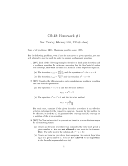
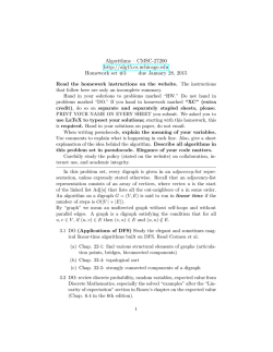


© Copyright 2026