1. Art and Diseño

Average-Case Competitive Analyses
for One-Way Trading
Hiroshi Fujiwara1
Toyohashi University of Technology
Kazuo Iwama
Kyoto University
Yoshiyuki Sekiguchi
Tokyo University of Marine Science and Technology
Abstract
Consider a trader who exchanges one dollar into yen and assume that the exchange rate
fluctuates within the interval [m, M ]. The game ends without advance notice, then the
trader is forced to exchange all the remaining dollars at the minimum rate m. El-Yaniv
et al. presented the optimal worst-case threat-based strategy for this game [EFKT01]. In
this paper, under the assumption that the distribution of the maximum exchange rate is
known, we provide average-case analyses using all the reasonable optimization measures
and derive different optimal strategies for each of them. Remarkable differences in behavior
are as follows: Unlike other strategies, the average-case threat-based strategy that minimizes
E[OPT/ALG] exchanges little by little. The maximization of E[ALG/OPT] and the minimization of E[OPT]/E[ALG] lead to similar strategies in that both exchange all at once.
However, their timing is different. We also prove minimax theorems with respect to each
objective function.
Keywords. Online Algorithms, Competitive Analysis, Average-Case Analysis, Stochastic
Analysis, Functional Analysis, Currency Trading, One-Way Trading, Financial Engineering.
1
Introduction
Since online competitive analysis was introduced, there has scarcely been any significant difference in attitude to worst-case performance
evaluation
ALG of online algorithms. Most studies use, as
or
min
their performance measure, max OPT
ALG
OPT for maximization problems, where ALG
and OPT denote the returns for maximization (the costs for minimization) of an online and an
optimal offline algorithms, respectively. (The difference between the two is not essential, both
are getting better with the quantity approaching to 1.0.) When it comes to average-case evaluation with an input distribution,
what is an
adequate
measure? A natural extension based on
ALG
E[OPT]
E[ALG]
,
E
,
,
or
expectations would be E OPT
ALG
OPT
E[ALG]
E[OPT] . It might seem that all of them are
reasonable and which one to be used is just a matter of taste. In this paper we warn that such
an easy choice is in fact quite dangerous by illustrating that the resulting optimal algorithm
varies crucially depending on which measure is adopted.
Our problem in this paper is one-way trading [EFKT01]. In this problem a trader owns
one dollar at the beginning and exchanges it into as much yen as possible, depending on the
exchange rate. We assume the range of the exchange-rate fluctuation is guaranteed to be on
[m, M ]. Note that the rate does not necessarily reach either m or M . The trader is allowed
to exchange an arbitrary amount of dollars to yen on each transaction but not allowed to get
dollars back. We also assume that the cost of sampling the exchange rate and the transaction
fees are negligible. There is a sudden end of the game at which the trader is obliged to exchange
all the remaining dollars at the possible lowest rate m. The trader is not informed in advance
when the game ends.
1
This work was partially supported by KAKENHI (16092216, 19700015, and 19740059).
1
s(r)
E[ALG/OPT]
1.4
E[OPT/ALG] (ATB)
1.2
1.0
max[OPT/ALG]
0.8
(WTB)
0.6
0.4
0.2
0.0
1
2
E[ALG]/E[OPT] & E[OPT]/E[ALG]
(i.e. E[ALG])
3
4
5
r
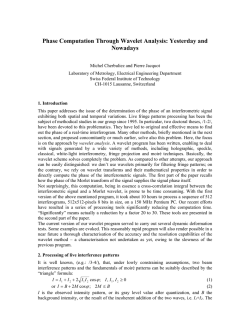
Figure 1: Optimal exchange strategies according to five different measures: The amount of
dollars s(r)dr to be exchanged when the exchange rate reaches r for the first time.
El-Yaniv et al. [EFKT01] presented the worst-case threat-based strategy WTB: (i) If the
q
current exchange rate q is the highest thus far, then the trader should exchange q0 sw (r)dr
1
for mcw ≤ r ≤ M and zero elsewhere, and q0 is the highest rate
dollars, where sw (r) = cw (r−m)
on the previous transaction. (ii) Otherwise, the trader should not exchange. cw is a constant
M −m
. Denoting the returns of an online and an optimal
determined by the equation c = ln m(c−1)
offline strategies
WTB minimizes the worst-case competitive
by ALG and OPT, respectively,
ALG (and
maximizes
min
).
They
also proved that randomization does not
ratio max OPT
ALG
OPT
help, i.e., the ratio cannot be improved even if the strategy is randomized. Thus there does not
seem any room for further improvement.
However, it is also true that worst-case analysis is often criticized as too pessimistic, and
average-case analysis has always been an interesting research target. For online algorithms
as well, several objective functions as presented above have recently appeared in the literature [FI05, PS06, Bec04, SSS06, NR08, GGLS08]. Our current problem involves a lot of human
activities; it seems especially interesting to make an analysis under proper input distributions.
1.1
Our Contribution
Our goal in this paper is average-case competitive analyses for one-way trading under several
input distributions and performance measures. Our first contribution is to show that the optimal
becomes
different depending on the performance measure, such as
ALGsignificantly
E[OPT]
strategy
E[ALG]
,
E
,
,
or
E OPT
ALG
OPT
E[ALG]
E[OPT] . Figure 1 illustrates the optimal amount of dollars to be
exchanged when the exchange rate reaches r for the first time, under the assumption that the
maximum rate of a game is uniformly distributed from between one and five. For comparison,
sw of the strategy WTB, independent of the distribution,
OPTis also drawn with a dashed line. (A)
One can easily distinguish the difference between E ALG and the others: Only the strategy
that minimizes E OPT
ALG , which we call the average-case threat-based strategy (ATB), exchanges
little by little on a certain rate range. In addition, ATB behaves differently also from WTB:
Whereas WTB waits for the possible maximum rate with keeping some dollars, ATB completes
the transaction
by the time the rate grows
up to 3.24. (B) Note that the minimization of
ALG
and
the
maximization
of
E
E OPT
ALG
OPT lead to different results. Recall that for worst-case
analysis it does not make sense to change max and min with taking reciprocal. Unlike ATB, the
2
ALG strategy that maximizes E OPT
is to exchange all at once at rate 2.67, which is drawn as a
E[ALG]
delta function in Figure 1. (C) The minimization of E[OPT]
E[ALG] and the maximization of E[OPT] are
essentially the same problem, i.e., the maximization of E [ALG], since E [OPT] is independent
of the online strategy. The result is to exchange all atonceat rate 3.00. We will prove that for
ALG
and that of E [ALG] result in such
an arbitrary distribution both the maximization of E OPT
one-time transaction. It is also shown that for
an
IFR
distribution
(for the definition please
ALG refer to Section 5), the exchange timing for E OPT is earlier than that for E [ALG].
We derive the performance of ATB and others all in closed form. This mathematically
nontrivial analysis itself is another important contribution of this paper. Firstly, for one-way
trading it is required to handle a function that describes a strategy, i.e. when and how much
to exchange, which obviously makes the analysis involved. Secondly, unlike other average-case
measures, this objective function is nonlinear: The return of an online strategy appears in the
denominator. El-Yaniv et al. gave some results on E [ALG],
are derived implicitly based
which
on the linearity [EFKT01]. We constructively analyze E OPT
with
the help of the calculus of
ALG
variations. More specifically, a subproblem over a smaller solution space is first solved. Then
we confirm the sufficient condition for the original problem.
1.2
Previous Work
Although the worst-case analysis introduced by Sleator and Tarjan [ST85] has provided us
with beautiful results in online computation, its limitation has also been revealed: (a) The
evaluation is often too pessimistic and therefore resulting optimal strategies seem far from
practical ones, for instance the optimal strategy for one-way trading is to wait for the possible
maximum rate with some dollars left. (b) In some cases the worst-case competitive ratio cannot
tell the performance difference properly, e.g. all of the algorithms LRU, FWF, and FIFO for
paging have the same worst-case competitive ratio despite the clear difference in empirical
ALG performance [BE98]. For supplementing these weak points, average-case analysis using E OPT
and so on has been recently proposed. Note that the expectation E [·] is taken with respect to
the input distribution.
ALG as a criterion of optimality
To overcome the weak point (a), [FI05] first employed E OPT
for designing strategies for the ski-rental problem and presented a family of optimal online
strategies which is different from that for worst-case analysis. The significant difference in
analysis between the ski-rent problem and one-way trading is as follows: Whereas a strategy
for the ski-rental problem is represented by a single real number which specifies when to buy
skis, for one-way trading, as mentioned, we need to determine a function for trading.
Other than the model that an input is drawn from a distribution that is known by the
online player in advance, several average-case models have been considered: Koutsoupias and
Papadimitriou introduced the diffuse adversary model in which the online player knows the class
of input distributions and the adversary attacks by choosing the worst distribution from the
class [KP94]. In the smoothed competitive analysis [BLMS+ 06], the input is probabilistically
distributed around a parameter selected by the adversary.
As for the difficulty (b), paging and online bin packing have been intensively studied. BecE[ALG]
[Bec04]. Shor
chetti showed the difference in performance between FWF and LRU using E[OPT]
studied the difference in the expected wasted spaces generated by the packing algorithms Best
Fit and First Fit, whose worst-case competitive ratios are the same [Sho86]. Please see [FW98]
for further results.
It seems itself of interest whether to take the expectation of ratios or the ratio of expectations. Panagiotou and Souza investigated
the performance of LRU for different cache size
E[ALG]
[PS06]. Conmeasures
more adequately than E[OPT]
and mentioned that in this case E ALG
OPT
3
ALG E[ALG]
cerning bin packing, in contrast, E OPT
make no difference as far as we consider
and E[OPT]
the asymptotic ratio for a sufficiently long input sequence [NR08]. Garg et al. recently pointed
E[ALG]
out the difference between E ALG
OPT and E[OPT] for the online Steiner tree problem: To obtain
ALG an upper bound of E OPT requires a scenario-wise comparison independently of results for
E[ALG]
E[OPT] [GGLS08].
In stochastic scheduling the processing time of a job is assumed to be a random variable
and therefore the performance of an algorithm has been measured based on average-case per[DLK82]. For stochastic complete-time scheduling Scharbrodt et al.
formance, usually E[ALG]
ALG E[OPT]
analyzed E OPT and illustrated its validity [SSS06]. Combining the conventional stochastic
scheduling and online optimization, Megow et al. proposed a stochastic online scheduling model
in which a job arrives online and its processing time is drawn probabilistically [MUV06].
El-Yaniv et al. introduced one-way trading in the context of online computation in their
conference paper [EFKT92]. They gave optimal strategies using worst-case analysis, as well as
some bounds of the worst-case competitive ratio. Al-Binali provided an optimal strategy in a
risk-reward framework in which the trader has an acceptable risk level and a forecast of the
exchange-rate fluctuation [al-99]. Iwama and Yonezawa generalized this framework in that they
introduced a below forecast and designed multi-phased strategies [IY99]. Chen et al. obtained
the worst-case competitive ratio in explicit form under the assumption that the exchange rate
approximately follows the geometric Brownian motion [CKLW01]. Lorenz et al. studied the
problem under the setting that at each point of time the trader chooses whether to convert a
fixed fraction of the initial wealth or to do nothing [LPS07]. Other models, including two-way
trading and portfolio selection, are mentioned in [BE98].
2
Preliminaries for the Calculus
First of all, we shall explain the motivation to apply Lebesgue integration
in this paper. The
most important objective of our work is to solve the minimization of E OPT
ALG . Unfortunately,
it seemed rather difficult to solve this problem directly. We thus began with some numerical
experiments to find an optimal over all finite sequences each of which describes a strategy.
Observing the results, we conjectured that a family of discontinuous functions achieves the
minimum. Therefore, we choose the function space L1 [m, M ] as a feasible set in order to deal
with such discontinuous functions comprehensively. L1 [m, M ] denotes the whole set of Lebesgue
M
integrable real-valued functions f on [m, M ] for which m |f (x)|dx < ∞ (see e.g. [Roy88]). We
also use the notation of C[m, M ] for the whole set of continuous real-valued functions on [m, M ].
We discuss Lebesgue-Stieltjes integration somewhere as needed. It is enough just to care
the treatment of discontinuous points as below. Let F be a non-decreasing function on [a, b]
that is discontinuous at c ∈ [a, b] and differentiable elsewhere, and g be a continuous function
on [a, b]. Denoting the derivative of F by f , we calculate
c
b
b
g(x)dF (x) =
g(x)f (x)dx +
g(x)f (x)dx + g(c)(F (c+) − F (c−)),
a
a
c
where F (c+) and F (c−) stand for lim→+0 F (c + ) and lim→+0 F (c − ), respectively. We will
use these notations throughout this paper.
Once again, our goal is to find a function that minimizes the functional E OPT
ALG . Let us
begin by describing a necessary condition for an extremum. The Gˆ
ateaux differential [Lue69]
of a functional J : L1 [m, M ] → R at f with increment v ∈ L1 [m, M ] is defined as
1
{J(f + v) − J(f )} .
→0 DJ(f )v := lim
4
A necessary condition for J to have an extremum at f¯ ∈ L1 [m, M ] is that
DJ(f¯)v = 0
holds for all v ∈ L1 [m, M ]. We usually proceed with our argument as follows: Suppose that
M
DJ(f¯)v is written as a form of m g(f¯, x)v(x)dx. Then, the fundamental lemma in variational
calculus implies that g(f¯, x) = 0 for all x ∈ [m, M ] (see e.g. [Lue69]).
Besides, we introduce the Kuhn-Tucker condition for the optimization of a functional with
inequality constraints. What one should note is, differently from the optimization over a finitedimensional vector space, the treatment of constraints over a real-valued domain. Suppose that
the constraint “f (x) ≥ 0 for all x ∈ [m, M ]” is added to the above example on J. Then, the
Kuhn-Tucker condition [Lue69] (i.e. a necessary condition) for the problem to have an extremum
at f¯ is that there exists μ ∈ L∞ [m, M ] such that
μ(x) ≤ 0 almost everywhere on [m, M ],
M
(1)
μ(x)f¯(x)dx = 0,
m
and
DJ(f¯)v +
M
μ(x)v(x)dx = 0
m
for all v ∈ L1 [m, M ]. (μ can be regarded as a Lagrange Multiplier for a finite-dimensional case.)
As far as this paper is concerned, it suffices to consider μ ∈ B[m, M ] ⊂ L∞ [m, M ] such that
instead of (1),
μ(x) ≤ 0 for all x ∈ [m, M ],
which is a stronger condition. B[m, M ] denotes the whole set of functions μ on [m, M ] for which
there exists K ∈ R such that |μ(x)| < K for all x ∈ [m, M ]. We thus omit to explain L∞ and
“almost everywhere”, which are not directly necessary in the later arguments. Please refer to
[Roy88] for further study on function spaces and measure theory.
3
Worst-Case Threat-Based Strategy
Recall that in our model the trader knows the possible range [m, M ] of the exchange-rate
fluctuation and does not know when the game ends. (In [EFKT01] this model is referred to
as Variant 2.) For convenience of calculus we assume that the exchange rate q(t) is piecewise
t+Δt
t+Δt
˜
˜
dS(t)
dollars into t
q(t)dS(t)
continuous with time t ≥ 0. The trader can exchange t
yen in an arbitrarily small time interval Δt. Thus the strategy of the trader is represented by
a function S˜ : [0, ∞) → [0, 1]. The rule of one-way transaction forces S˜ to be a non-decreasing
function. Suppose that the game is over at time τ . Then the trader has to exchange the
remaining dollars at the minimum rate m. The total return is written as
τ
τ
τ
˜
˜
˜
q(t)dS(t) + m 1 −
dS(t) = m +
(q(t) − m) dS(t).
ALGS˜ (τ ) =
0
0
0
On the other hand, the optimal offline strategy will exchange the whole one dollar at the highest
rate throughout the game and therefore its return is OPT(τ ) = max0≤x≤τ q(x).
El-Yaniv et al. stated that it is sufficient to consider strategies that exchange only when the
exchange rate is the highest so far [EFKT01]. Let q¯(t) denote max0≤x≤t q(x). Such a strategy
q(t+Δt)
dS(r) dollars if q(t + Δt) > q¯(t) and does not exchange otherwise, where
exchanges q¯(t)
5
S : [m, M ] → [0, 1] is a non-decreasing function. We distinguish between these two categories
of strategies by denoting S˜ and S; strategies with respect to time and those with respect to
the highest exchange rate. We also describe a strategy with respect to the exchange rate by
s(r) := dS(r)
dr if the derivative of S exists. Suppose that the highest exchange rate of the game
is p. Without loss of generality, we assume q(0) = m. The return is obtained as
p
p
p
ALGS =
rdS(r) + m 1 −
dS(r) = m +
(r − m) dS(r).
m
m
m
Obviously, the optimal offline strategy gains OPT = p. We later denote ALGS simply by ALG
when S is clear from the context. Here we present the (worst-case) threat-based strategy proposed
M −m
.
by El-Yaniv et al. Let cw be the root of the equation c = ln m(c−1)
Strategy WTB Suppose that the exchange rate changes from q(t) to q(t + Δt). (i) If q(t +
q(t+Δt)
sw (r)dr dollars, where
Δt) > q¯(t) then exchange q¯(t)
sw (r) =
1
cw (r−m) ,
0,
mcw ≤ r ≤ M ;
m ≤ r < mcw .
(ii) If q(t + Δt) ≤ q¯(t) then do not exchange.
Theorem 1 ([EFKT01]). For any q, the strategy WTB minimizes the worst-case competitive
OPT(τ )
to cw .
ratio maxτ ALG
˜ (τ )
S
4
Average-Case Threat-Based Strategy
We consider the model in which the highest exchange rate until a game is over follows a probability distribution and the trader devises a strategy with help of the knowledge of it. A distribution
is characterized by a cumulative distribution function F : [m, M ] → [0, 1] such that F (p) is the
probability that the highest exchange rate of the game is equal to or less than p. Throughout
this paper, E[·] denotes the expectation with respect to F unless otherwise specified as EH [·]
for a distribution H. We will seek an optimal online strategy that minimizes
M
p
OPT
p
dF (p)
=
E
ALG
m m + m (r − m)dS(r)
among those that exchange only when the exchange rate is the highest so far.
Lemma 2 claims that it suffices to consider such a family of strategies, as it is the case
in the worst-case analysis. More specifically, if the highest exchange rate is drawn from a
distribution, an optimal strategy with respect to the highest exchange rate is also optimal
among those with respect to time which may exchange even not at the highest rates. As the
same as in Section 3, let q be a rate function of time and q¯(t) := max0≤x≤t q(x). For a given q,
let D := {t : 0 ≤ ∃x < t, q(x) ≥ q(t)}, i.e., the set of time instant at which the current rate is
not the highest so far. We begin with a lemma that any strategy with respect to time can be
converted into one that exchanges only at the highest rates without reducing its gain. Please
recall that a strategy with (without) a tilde denotes one with respect to time (the highest
exchange rate, respectively).
Lemma 1. For any q and any strategy S˜0 , there exists a strategy S˜ such that S is constant on
D and ALGS˜ (τ ) ≥ ALGS˜0 (τ ) for all τ ≥ 0.
6
Proof. One can see that D consists of a family of disjoint intervals, which are labeled as
D1 , D2 , . . . , Dl . Let us set ai = inf Di and bi = sup Di for all 1 ≤ i ≤ l. For each Di , one
can choose zi ∈
/ D such that q(zi ) ≥ supx∈Di q(x) and zi ≤ ai . We compose S˜1 , S˜2 , . . . , S˜l from
S˜0 by
⎧
˜
˜
˜
⎪
⎨Si−1 (t) + Si−1 (bi ) − Si−1 (ai −), zi ≤ t < ai ;
S˜i (t) = S˜i−1 (bi ),
ai ≤ t < bi ;
⎪
⎩˜
0 ≤ t < zi , bi ≤ t.
Si−1 (t),
for 1 ≤ i ≤ l. It follows that
bi
˜
(q(t) − m) dSi−1 (t) ≤ sup q(x) − m · S˜i−1 (bi ) − S˜i−1 (ai −)
lim
→+0 a −
x∈Di
i
≤ (q(zi ) − m) · S˜i−1 (bi ) − S˜i−1 (ai −)
zi
(q(t) − m) dS˜i (t).
= lim
→+0 z −
i
Since each zi is a lower bound of Di , we have for all τ ≥ 0,
τ
τ
˜
˜
(q(t) − m) dS0 (t) ≤
(q(t) − m) dS1 (t) ≤ · · · ≤
0
0
τ
0
(q(t) − m) dS˜l (t).
˜ the proof is completed.
By adding m for each and rewriting S˜l as S,
Given a distribution F and a rate function q, consider a distribution H : [0, ∞) → [0, 1]
defined as H(t) := F (¯
q (t)) for all t ≥ 0. Then, one can observe that H(t) is the probability that
the game ends by the time t, since F (p) is the probability that (the highest exchange rate) ≤ p.
Indeed, H increases while the exchange rate hits a new high, and remains constant otherwise.
∗
Lemma 2. Suppose that there
exists a strategy S such that EF [OPT/ALGS ∗ ] ≤ EF [OPT/ALGS ]
holds for all S. Then, EH OPT(t)/ALGS˜∗ (t) ≤
˜ where S˜∗ (t) := S ∗ (¯
q (t)) for all t ≥ 0.
EH OPT(t)/ALGS˜ (t) for all S,
Proof. Assume that there exists S˜0 such that
EH
OPT(t)
OPT(t)
> EH
.
ALGS˜∗ (t)
ALGS˜0 (t)
Since H and S˜∗ are constant on D by definition, we have
OPT(t)
OPT(t)
=
dH(t)
EH
ALGS˜∗ (t)
[0,∞)\D ALGS˜∗ (t)
OPT(t)
dF (¯
q (t))
=
ALG
[0,∞)\D
S˜∗ (t)
M
OPT
dF (p)
=
m ALGS ∗
OPT
,
= EF
ALGS ∗
7
where p := q¯(t). On the other hand, Lemma 1 implies that there exists S˜ such that S˜ is constant
on D and
OPT(t)
OPT(t)
≥ EH
.
EH
ALGS˜0 (t)
ALGS˜ (t)
˜ for all t ≥ 0. Arguing similarly to above we obtain
Consider S defined as S(¯
q (t)) := S(t)
OPT(t)
OPT
= EF
.
EH
ALGS˜ (t)
ALGS
Thus we have
EF
OPT
ALGS ∗
> EF
OPT
,
ALGS
which contradicts the optimality of S ∗ .
As a result of the analysis in Section 4.3 we obtain an optimal strategy, which we name
the average-case threat-based strategy (ATB). This strategy advises to exchange dollars only
during a certain exchange-rate range of [α, β] ⊂ [m, M ]. In what follows we assume that the
distribution F has a positive density function f .
Strategy ATB Suppose that the exchange rate changes from q(t) to q(t + Δt). (i) If q(t +
q(t+Δt)
sa (r)dr dollars, where
Δt) > q¯(t) then exchange q¯(t)
⎧
⎨
sa (r) =
⎩
m
√
(α−m) αf (α)
3r−m
2(r−m)
f (r)
r
+
f (r)
2
r
f (r)
0,
,
α ≤ r ≤ β;
(2)
otherwise.
(ii) If q(t + Δt) ≤ q¯(t) then do not exchange. α and β are constants given by
M
β
sa (r)dr = 1 and β(β − m)f (β) =
pf (p)dp.
α
(3)
β
Given f , one can have the value of β from the second equation in (3). The value of α is determined by the first equation in (3) after substituting sa with α unknown. The optimality of
ATB requires the Condition (C) which appears in Lemma 4. A simple sufficient condition for
(C) is the following (C).
f is non-decreasing on [m, β] and (r − m)2 rf (r) ≥ (β − m)2 βf (β) holds for all r ∈ [β, M ].
(C)
Examples of ATB for several distributions will follow shortly before showing the optimality.
4.1
Uniform Distribution
1
Consider the probability density function f (p) = M −m
, which means that the highest rate p is
uniformly distributed on the range [m, M ]. The optimal online strategy ATB is then represented
by
m√
· 3r−m√ , α ≤ r ≤ β;
sa (r) = (α−m) α 2(r−m) r
0,
otherwise.
√
We derive β = 13 m + m2 + 3M 2 < m + 23 (M − m) from (3). (The other root is negative
Note that the uniform
and therefore infeasible.) One can easily confirm the Condition (C).
8
OPT/ALG
s(r)
2.2
8
2.0
6
E[OPT/ALG] (ATB)
max[OPT/ALG] (WTB)
1.8
E[OPT/ALG] (ATB)
1.6
4
max[OPT/ALG] (WTB)
1.4
2
0
1.0
1.2
1.2
1.4
1.6
1.8
2.0
1.0
r
2
4
6
8
10
r
Figure 3: Performance ratios of ATB
and WTB for a uniform distribution
(M/m = 1 to 10).
Figure 2: ATB and WTB for a uniform
distribution.
distribution means that we have a completely even chance of the highest exchange rate in the
range. This allows us to concentrate on rather narrow range for trade, which is obviously
impossible if we assume the worst-case adversary. Actually, the above inequality implies that
ATB completes the conversion before the rate reaches 66% of the range [m, M ]. Figure 2
illustrates the case of m = 1 and M = 2. When ATB finishes the entire transaction, WTB
still retains 48% of the initial asset. Moreover, WTB waits with some dollars left until the
exchange rate finally reaches M , no matter how scarcely the luck happens. The advantage of
ATB appears in the
measure: By exchanging dollars intensively
OPT on a narrow range
performance
=
E
is
improved
down
to
1.20
from
1.29
(=
c
of [1.38, 1.53], E OPT
w
ALG
WTB ). For the setting
of m = 1 and M = 10, the improvement
is
1.88
from
2.10
by
making
transaction
on the range
OPT OPT [2.8, 6.1]. Figure 3 illustrates E ALG and max ALG for M/m = 1 to 10.
4.2
Extreme Value Distribution
If random variables are independent and identically distributed then the maxima under some
affine transformation follow the generalized extreme value distribution [Ger89, EKM97]
1
1
p − μ −1− k
p − μ −k
1
1+k
exp − 1 + k
.
f (p) =
σ
σ
σ
Apparently, this distribution provides the trader with useful information on the exchange rate.
Consequently, the degree of improvement is outstanding compared with that of the uniform
distribution. Again, let m = 1 and M = 2. Recall that the value of cw is 1.29 previously. (i)
Weibull distribution, say, k = −0.5, σ = 0.12, μ = 1.77 (see Figure 4): The density function has
a peak at 1.84 and a long tail to the left. That is, the trader is informed
that the rate is in an
is
reduced
down to 1.15.
upward trend. ATB exchanges on the range [1.59,1.66] and E OPT
ALG
(ii) Fr´echet distribution, say, k = 0.5, σ = 0.2, μ = 1.39
This setting satisfies the Condition (C).
(see Figure 5): This setting yields a right-tailed distribution whose peak is at 1.32. The trader
anticipates
that
the rate does not grow so much. ATB converts dollars on the range [1.27,1.34]
becomes
1.19. One can confirm the Condition (C).
and E OPT
ALG
9
s(r), f(r)
s(r), f(r)
20
20
E[OPT/ALG] (ATB)
15
15
f
E[OPT/ALG] (ATB)
10
10
f
5
0
1.0
5
1.2
1.4
1.6
1.8
Figure 4: ATB for a Weibull distribution.
4.3
2.0
r
0
1.0
1.2
1.4
1.6
1.8
2.0
r
Figure 5: ATB for a Fr´echet distribution.
Proof of Optimality
The proof of the optimality involves the calculus of variations. The minimization of E
can be written as:
M
pdF (p)
p
(P) minimize J(s) :=
m
+
m
m (r − m)s(r)dr
M
s(r)dr = 1, s(r) ≥ 0, s ∈ L1 [m, M ].
subject to
OPT ALG
m
Outline of the proof We first provide a sufficient condition for global optimality for (P).
Next we consider a subproblem (P0 ) over a smaller solution space. Starting from a necessary
condition for (P0 ), we derive a local optimal solution. Finally, it is confirmed that the obtained
solution satisfies the sufficient condition for the original problem (P).
Lemma 3. Suppose that there exist feasible s¯ ∈ L1 [m, M ], λ ∈ R and μ ∈ B[m, M ] such that
M
s(r)dr = 0 and
μ(r) ≤ 0 for all r ∈ [m, M ], m μ(r)¯
p
M
M
M
−p m (r − m)v(r)dr
λv(r)dr +
μ(r)v(r)dr = 0
(4)
2 dF (p) +
p
m
m
m
s(r)dr
m + m (r − m)¯
for all v ∈ L1 [m, M ]. Then s¯ is a unique solution to the problem (P).
Proof. The objective function is Gˆ
ateaux differentiable on the feasible set with the derivative
DJ(s) given by
p
M
−p m (r − m)v(r)dr
DJ(s)v =
2 dF (p)
p
m
s(r)dr
m + m (r − m)¯
1
is strictly convex on [0, ∞), we can show that J is strictly
for each v ∈ L1 [m, M ]. Since 1+x
convex on the convex feasible set. Indeed, for any two different strategies s1 and s2 in the feasible
set and any 0 < γ < 1, J(γs1 + (1 − γ)s2 ) < γJ(s1 ) + (1 − γ)J(s2 ) holds. Hence, it follows that
M
M
for each feasible s, J(s) ≥ J(¯
s) + DJ(¯
s)(s − s¯). Also, m s(r)dr = 1 and m μ(r)s(r)dr ≤ 0,
10
since μ(r) ≤ 0 for all r ∈ [m, M ] as assumed. Then we have for each feasible s
J(s) ≥ J(s) + λ
M
s(r)dr − 1 +
m
≥ J(¯
s) + DJ(¯
s)(s − s¯) + λ
M
μ(r)s(r)dr
m
M
(s(r) − s¯(r))dr +
m
M
μ(r)(s(r) − s¯(r))dr
m
= J(¯
s) + (DJ(¯
s) + λ + μ)(s − s¯)
= J(¯
s).
M
M
s(r)dr = 0,
Therefore s¯ is a minimizer of the problem (P). Note that m s¯(r)dr = 1 and m μ(r)¯
and that we derive the last equality by applying (4).
M Suppose s0 also attains the minimum. Then the equalities hold in each relation above. Thus
¯.
m μ(r)s0 (r)dr = 0 and the strict convexity of J ensures that s0 = s
Note In Lemma 3, it is mathematically more natural to consider L∞ [m, M ] that is the dual
space of L1 [m, M ] than B[m, M ], which requires the knowledge of functional analysis. The
condition in this lemma then corresponds to the Kuhn-Tucker condition [Lue69]. To consider
B[m, M ] ⊂ L∞ [m, M ] is sufficient for our arguments and therefore we do so.
implies the following condition (C).
Lemma 4. The Condition (C)
(C)
α
pf (p)dp ≥ 0, ∀r ∈ [m, α];
α(α − r)(α − m)f (α) − (r − m)
r
(3r − m)f (r) + (r − m)rf (r) > 0,
M
2
pf (p)dp ≥ 0,
β(β − m) f (β) − (r − m)
∀r ∈ (α, β);
∀r ∈ [β, M ].
r
implies that f (r) ≥ 0 for all r ∈ [m, β]. Therefore the second
Proof. The Condition (C)
α
inequality straightforwardly holds. Let g(r) = α(α − r)(α − m)f (α)
−
(r
−
m)
r pf (p)dp. By
α
differentiating we have g (r) = −α(α − m)f (α) + r(r − m)f (r) − r pf (p)dp. Again, g (r) =
(3r − m)f (r) + (r − m)rf (r), which is positive. Together with g (α) = 0, it follows that
g (r) ≥ 0 for all r ∈ [m, α]. Since g(α) = 0, we obtain the first inequality. By applying
M
rf (r) ≥ (β − m)2 βf (β)/(r − m)2 , we have β(β − m)2 f (β) − (r − m) r pf (p)dp ≥ (r − m)(β −
m)2 βf (β)/(M − m) > 0 for all r ∈ [β, M ], which is sufficient for the third inequality.
Theorem 2. Suppose that a distribution F has a density function f which is positive, continuously differentiable, and satisfies the Condition (C). Then the unique minimizer of the problem
(P) is sa in (2). The constants are given by (3).
Proof. First, we narrow the candidates of solutions to functions which are nonnegative and
continuous on a subinterval of [m, M ] and zero elsewhere. Then the problem finding a minimizer
11
from such family of functions has the following form:
(P0 ) minimize J0 (s, α, β)
β
α
pf (p)
pf (p)dp
p
dp +
:=
m
m
+
m
α
α (r − m)s(r)dr
M
pf (p)dp
;
+
β
β
m + α (r − m)s(r)dr
β
subject to G(s, α, β) :=
s(r)dr = 1, s(r) ≥ 0, m < α < β < M,
α
s ∈ C[m, M ].
Observe the problem (P0 ) is no longer a convex program. Thus we find a function s¯ which
satisfies a necessary condition for local optimality in (P0 ). Then we will confirm the condition
in Lemma 3 by explicitly giving a constant λ and a function μ there.
Suppose (¯
s, α, β) is a local optimal of (P0 ) and s¯ is positive. Then there exists λ ∈ R such
that
s, α, β)(v, ξ, η) + λDG(¯
s, α, β)(v, ξ, η) = 0
(5)
DJ0 (¯
for all ξ, η ∈ R, v ∈ C[m, M ]. Here
s, α, β)(v, ξ, η)
DJ0 (¯
⎫⎤
⎡⎧
M
⎪
⎪
⎨ β (α − m)¯
(α − m)¯
s(α) β pf (p)dp ⎬⎥
s(α)pf (p)dp
⎢
=⎣
2 ⎦ ξ
2 + p
β
⎪
⎪
s(r)dr
⎩ α m + α (r − m)¯
s(t)dt ⎭
m + α (t − m)¯
⎫
⎧
p
⎪
⎪
β
⎬
⎨ (β − m) M pf (p)dp
−pf (p) α (r − m)v(r)dr
β
+ 2 s¯(β) η +
2 dp
p
⎪
⎪
α
(r
−
m)¯
s
(r)dr
m
+
⎭
⎩ m + β (r − m)¯
s(r)dr
α
α
β
M
−pf (p) α (r − m)v(r)dr
+
2 dp
β
β
s(r)dr
m + α (r − m)¯
and
DG(¯
s, α, β)(v, ξ, η) = s¯(β)η − s¯(α)ξ +
β
v(p)dp.
α
By substituting ξ = η = 0 in (5), we have
p
β
β
β
−pf (p) α (r − m)v(r)dr
dp
+
A
·
(r
−
m)v(r)dr
+
λ
v(p)dp = 0,
2
p
α
α
α
s(t)dt
m + α (t − m)¯
where
M
− β pf (p)dp
A= 2 .
β
s(t)dr
m + α (t − m)¯
We change the order of the integration of the first term and replace p with r in the third
term. Then we obtain
$
β
β
−pf (p)dp
v(r) (r − m)
2 + A + λ dr = 0.
p
α
r
s(t)dt
m + α (t − m)¯
12
The fundamental lemma in variational calculus states that if the equation holds for every v ∈
C[m, M ], then
β
−pf (p)dp
(6)
(r − m)
2 + A + λ = 0
p
r
s(t)dt
m + α (t − m)¯
for all r ∈ [α, β]. By substituting r = β and r = α in (6), we have respectively (α − m)B + (α −
m)A + λ = 0 and (β − m)A + λ = 0, where
β
B=
α
We also have
β
r
−pf (p)dp
2 .
p
s(t)dt
m + α (t − m)¯
rf (r)
−pf (p)dp
2 + (r − m) 2 + A = 0
p
r
s(t)dt
s(t)dt
m + α (t − m)¯
m + α (t − m)¯
(7)
by differentiating (6) and hence
B+
(α − m)αf (α)
+A=0
m2
by letting r = α. Thus we obtain
λ=
(α − m)2 αf (α)
.
m2
Then we eliminate the first term in (6) and (7) and hence
(r − m)2 Thus we obtain
m+
r
rf (r)
α (t
− m)¯
s(t)dt
2 − λ = 0.
%
1
(t − m)¯
s(t)dt = √ (r − m) rf (r),
λ
α
since the left hand side should be positive. By differentiating we have
$
&
&
3r − m
f (r) f (r)
r
1
+
.
s¯(r) = √
r
2
f (r)
λ 2(r − m)
r
m+
(8)
(9)
The second inequality in the Condition (C) guarantees its feasibility. Now let us determine α
and β. By substituting β for r in (7), we have
β(β − m)f (β) =
M
pf (p)dp,
β
β
which is the condition for β. Then, α is determined by α s¯(r)dr = 1 and (9). Therefore we
have shown that s¯ is equal to sa .
To complete the proof, we use Lemma 3 to show the obtained function to be a minimizer
of the original problem (P). By substituting s¯ for s in (4) and changing the order of the
13
integration, we have
α
v(r)
m
1
m2
α
−(r − m)
pf (p)dp + α(α − r)(α − m)f (α) + μ(r) dr
r
·
λ
β(β − m)2 f (β)
β
α
M
v(r)μ(r)dr +
+
v(r)
β
M
−(r − m)
pf (p)dp + β(β − m)2 f (β) + μ(r) dr
r
= 0.
Suppose now the Condition (C) is satisfied. Observing the first and third terms in the above
equality, we can choose μ(r) ≤ 0 for all r ∈ [m, α] and r ∈ [β, M ], respectively, so that each
term is equal to zero for any v ∈ L1 [m, M ]. The second term also becomes zero by setting
μ(r) = 0 for all r ∈ (α, β). We have thus confirmed that (4) is satisfied by obtained s¯, λ, and
μ.
4.4
Randomized Strategies
The following result by El-Yaniv et al. shows that randomization of one-way trading strategies'cannot improve
(
'EG [RALG]
( nor therefore the average-case performance measure such as
EG [RALG]
OPT
, or EF [EG [RALG]], where EG [RALG] denotes the expected
EF EG [RALG] , EF
OPT
return of a randomized strategy RALG. It is also mentioned that in one-way trading there is
no essential difference between the two types in randomized strategies; a mixed strategy that is
represented by a distribution over a class of deterministic strategies and a behavioral strategy
that randomly determines the amount of dollars to be exchanged at every time.
Proposition 1 ([EFKT01]). Let RALG be any randomized strategy which may be a mixed
or behavioral strategy. Then, there exists a deterministic strategy represented by S such that
EG [RALG] = ALGS for any scenario of the exchange-rate fluctuation. The reverse statement
also holds true: For any deterministic strategy represented by S, there exists a randomized
strategy RALG which satisfies the above equality.
4.5
Minimax Theorem
Online problems are usually handled as a game between an online player and an adversary.
In our model the adversary selects a distribution and after that the online player determines
the strategy. That is, the adversary cannot make any adaptive choice. Nevertheless, the next
theorem states that even this type of adversary can attack the player as cruelly as the one who
devises a strategy after observing the online player’s decision.
Theorem 3.
OPT
OPT
= min max E
= cw .
max min E
F ALG
ALG F
ALG
ALG
A remarkable point here is that we find a saddle point:
and
⎧
⎪
⎨0,
w −1)
cw −1
w
ln m(c
Fw (p) = cp−mc
2 (p−m) −
p−m ,
c2w
w
⎪
⎩
1,
14
sw (r) in (3), i.e., the strategy WTB
p ∈ [m, mcw );
p ∈ [mcw , M );
p = M.
(10)
In other words, Fw represents the strongest adversary in our model.
One should note that one-way trading in this paper is an infinite game. For a finite game,
Yao’s principle that is derived from Loomis’ lemma [MR95] provides a lower bound of the worstcase competitive ratio of randomized algorithms [BE98]. Indeed, if we narrow F and RALG
down to distributions over finite strategies such that RALG includes WTB, then an
upper
=
bound of can be given as follows: According to Loomis’ lemma, maxF minALG EF OPT
ALG
OPT implies that the right-hand-side equals
minG maxp E
' G RALG (. Jensen’s inequality
OPT OPT
minG maxp EG [RALG] = minALG maxp ALG = cw , which is equivalent to the first equality in
Theorem 3. However, our model treats uncountable strategy sets consisting of functions and
distributions, for which Loomis’ lemma does not hold. Theorem 3 is obtained independently
with a constructive discussion. Another example that derives a special case of Yao’s principle
for an infinite game with a countable strategy set can be found in [BE98]. Also note that unlike
other minimax theorems Theorem 3 holds for a noncompact strategy set.
Proof. Firstly, we prove minALG maxF E OPT
ALG = cw . We set the cumulative distribution function Fx (p) = 1 for p ∈ [x, M ] and zero for p ∈ [m, x) with x chosen after the online strategy is
revealed. This is equivalent to the adversary in a worst-case analysis. Therefore a lower bound
is cw . On the other hand, by substituting strategy sw of WTB the lower bound is achieved from
Theorem 1.
Secondly, we show maxF minALG E OPT
ALG = cw . The sketch of the proof is as follows. We
have already known that ATB minimizes for distributions satisfying the Condition (C). We
begin with formally applying ATB. Then we first maximize the objective functional over a
particular subset of distributions. In fact, we consider a subspace including a given distribution
F0 as a feasible set. Then a parametric optimization problem is obtained with F0 being the
parameter. We find a parameter for which the optimal value coincides with cw . Finally, we
confirm that the obtained optimal solution is an optimal for the original problem, by applying
Lemma 3.
Let us fix a distribution F0 that has a density function f0 . We formally substitute sa of
ATB for s. Then the function to be maximized is
M
β
α
pf0 (p)
pf0 (p)
pf0 (p)
%
%
dp +
dp.
dp +
1
1
m
√ (β − m) βf0 (β)
m
α √ (p − m) pf0 (p)
β
λ
λ
2
Note that we employed (8) instead of substituting sa directly and that λ = (α−m)m2αf (α) . Then,
for given α, β, and F0 , consider F that is equal to F0 on [m, α] and smooth on (α, M ). Then
the maximization problem is
β
m
p
pf (p)
%
%
dp
dF (p) +
m
(α − m) αf (α) α (p − m) pf (p)
m
M
pf (p)
m
%
%
dp
+
(α − m) αf (α) β (β − m) βf (β)
mM (F (M ) − F (M −))
%
;
+
(α − m)(β − m) αβf (α)f (β)
M
dF (p) = 1
subject to
α
maximize I(F ) :=
m
dF (p) > 0, p ∈ (α, M ]
F (p) = F0 (p), p ∈ [m, α],
15
where f is the function on [α, β] defined by
⎧
⎪
⎨F (α+),
f (p) = F (p),
⎪
⎩ F (β−),
p = α;
p ∈ (α, β);
p = β.
If the problem has an optimal F¯ , the Kuhn-Tucker theorem guarantees the existence of η ∈ R
such that F¯ also maximizes the functional
M
I(F ) + η
dF (p) − 1
m
over all F with dF (p) > 0 and F (p) = F0 (p) on [m, α]. Let us consider a set W of variations
such that every w ∈ W is nonzero on (α, β) and zero elsewhere. By considering the Gˆ
ateaux
differential of the above functional, we have
$
β
p
m
%
%
+ η dp = 0
w(p)
(α − m) αf¯(α) 2(p − m) pf¯(p)
α
for all w ∈ W , where f¯ is defined similarly by F¯ . The fundamental lemma in variational calculus
states that
p
m
%
%
+η =0
(11)
¯
(α − m) αf (α) 2(p − m) pf¯(p)
holds for all p ∈ (α, β). Then we obtain
p
(α − m)2 αf¯(α)
f¯(p) =
2
2
m
4η (p − m)2
for all p ∈ [α, β]. Letting p = α yields η = −α/(2m), since η should be nonpositive for satisfying
the equation (11).
By applying (8) to (11) again, we have
α
p
p
= −2η = .
(12)
m
m + α (r − m)s(r)dr
Note that s here is a strategy formally optimized with leaving α and β to be original for F0 .
Suppose that we have chosen F0 such that α ≤ mcw and β = M . Now let us remind ourselves
of WTB. If we substitute sw of WTB for s, then the left hand side of (12) is constant for
p ∈ [mcw , M ], which implies that sw is a candidate for s. In order for sw to be a solution, it is
necessary to choose F0 so that α/m = cw . In what follows, assume that we have chosen such
F0 .
We next adjust the undetermined quantities F¯ (M ) − F¯ (M −) and f¯(α) in the obtained
distribution so that the optimality of WTB is consistent for this distribution. So, we set
M
F¯ (M ) − F¯ (M −) to satisfy M (M − m)f¯(M ) = β pdF¯ (p) = M (F¯ (M ) − F¯ (M −)), which is
obtained by applying slightly modified arguments in Theorem 2 to the case β = M . Since F¯ is
a probability distribution, we have
M
α
¯
dF (p) +
f¯(p)dp + F¯ (M ) − F¯ (M −)
1=
m
α
α
M −m
m
m
(α − m)2 f¯(α)
ln
−
+
dF0 (p) +
=
α
α−m
M −m α−m
m
(α − m)2 f¯(α) M
.
+
α
M −m
16
M −m
Recall that cw = ln m(c
and α = mcw . Then,
w −1)
f¯(α) = (1 − K)
where K =
α
m dF0 (p).
α
,
(α − m)2
Eliminating f¯(α) we have
p
m(α − m)
;
f¯(p) = (1 − K)
α2
(p − m)2
m(α − m) M
.
F¯ (M ) − F¯ (M −) = (1 − K)
α2
M −m
Now we set F0 (p) = 0 on [m, α) and F0 (α) = K. Then we obtain I(F¯ ) = cw . Therefore if we
can show that WTB is in fact an optimal when K = 0, it completes the proof.
By applying Lemma 3 to the distribution above, it is sufficient to show that sw satisfies
m(α − m)
α2
β
α
p
−p2 m (r − m)v(r)dr
2 dp
p
(p − m)2 m + α (r − m)sw (r)dr
p
−M m (r − m)v(r)dr
m(α − m) M
+
2
M
α2
M −m
m + α (r − m)sw (r)dr
M
+
λv(r)dr +
m
α
m
−(α − m)
v(r)(r − m)dr +
m
α
M
v(r)dr +
Thus we can choose λ = (α − m)/m and
μ(r) =
M
M
m
μ(r)sw (r)dr = 0.
M
λv(r)dr +
m
μ(r)v(r)dr = 0,
m
for some λ ∈ R and μ ∈ B[m, M ] with μ(r) ≤ 0 for all r ∈ [m, M ] and
The above equation is simplified as
1
−
m
M
μ(r)v(r)dr = 0.
m
− α−r
m , r ∈ [m, α];
0,
r ∈ (α, M ]
so that the equality holds. Therefore WTB is an optimal for the obtained distribution and the
proof is completed.
5
Optimal Strategies for Other Measures
In this section we analyze E
ALG OPT
E[OPT]
E[ALG]
E[ALG] and E[OPT] need not to
E[ALG]
maximization of E[OPT]
are both equivalent
and E [ALG]. Note that
be considered; the minimization of E[OPT]
E[ALG] and the
to the maximization of E [ALG], since E [OPT] is independent
of the online strategy. Before
ALG and E [ALG], it suffices to concendiscussing optimal strategies, we claim that also for E OPT
trate on strategies which exchange only when the exchange rate is the highest so far. We give
the following two lemmas without proofs, which can be shown similarly to Lemma 2. We use
q (t)) for all t ≥ 0.
the same notation as in Section 4. For a given strategy S ∗ , let S˜∗ (t) := S ∗ (¯
Besides, one should recall that randomization does not help for either measures as mentioned
in Proposition 1.
17
∗
Lemma 5. Suppose that there
exists a strategy S such that EF [ALGS ∗ /OPT] ≥ EF [ALGS /OPT]
holds for all S. Then, EH ALGS˜∗ (t)/OPT(t) ≥
˜
EH ALGS˜ (t)/OPT(t) for all S.
Lemma 6. Suppose that there exists a strategy S ∗ such that EF [ALGS ∗ ] ≥ EF [ALGS ] holds
˜
for all S. Then, EH ALGS˜∗ (t) ≥ EH ALGS˜ (t) for all S.
Unlike the minimization of E OPT
, we can show that for any distribution, both the maxiALG
ALG mization of E OPT and that of E [ALG] lead to an optimal strategy that exchanges the whole
one dollar at a certain timing. Such a strategy is referred to as RPP in [EFKT01], in which the
maximization of E [ALG] is discussed.
We also mention the case that the given distribution belongs to a class of distributions,
called IFR. According to [Ger89], we define IFR on [m, M ] as follows.
Definition. A distribution F is said to be in IFR if f (p)/(1− F (p)) increases for all p ∈ [m, M ],
where f is the density function of F .
This class includes a comprehensive family of distributions such as the uniform, the normal,
or a special case of Weibull distributions. For adistribution F ∈ IFR, we prove that the optimal
timing of the one-time transaction for E ALG
OPT is earlier than that of E [ALG].
ALG ,
Theorem 4. The strategy S1 (r) = 1 for r ∈ [r1 , M ] and zero elsewhere maximizes E OPT
M dF (p)
where r1 < M is a maximizer of (r − m) r
p .
Proof. By changing the order of the integration, we have
p
M
m + m (r − m)dS(r)
ALG
=
dF (p)
E
OPT
p
m
M
M
M
dF (p)
dF (p)
+
dS(r)
(r − m)
=m
p
p
m
m
r
M
M
dF (p)
dF (p)
+ max
.
(r − m)
≤m
m≤r≤M
p
p
m
r
There exists r1 < M which achieves the maximum and then the maximum of E
attained for given S1 .
ALG OPT
is also
Theorem 5 ([EFKT01]). The strategy S0 (r) = 1 for r ∈ [r0 , M ] and zero elsewhere maximizes
E [ALG], where r0 is a maximizer of (r − m)(1 − F (r)).
Proposition 2. If F ∈ IFR, then r1 < r0 .
Proof. Let g(r) := (r − m)(1 − F (r)) and h(r) := (r − m)
M
r
dF (p)
p .
We have the derivative
f (r)
g (r) = 1 − F (r) − (r − m)f (r) = (1 − F (r)) 1 − (r − m)
1 − F (r)
.
f (r)
Since 1−F
(r) is an increasing function, the sign of g (r) turns only once from positive to negative
as r grows, or remains nonnegative. Therefore g(r) has a unique peak or is a non-decreasing
M
function. We also have h (r) = r dFp(p) − (r − m) f (r)
r . Since r1 is a maximizer of h and
18
h (m) > 0, h (r1 ) is zero. Thus
g (r1 ) = 1 − F (r1 ) − (r1 − m)f (r1 )
M
M
dF (p)
dF (p) − r1
=
p
r1
r1
M
p − r1
dF (p)
=
p
r1
> 0,
which implies that g(r) achieves the maximum in (r1 , M ].
We give some numerical results for distributions which have already
ALG appeared as examples.
and E [ALG], respecAs above theorems, let r1 and r0 denote the optimal timings for E OPT
tively. For the uniform distribution with m = 1 and M = 2, we have r1 = 1.46 and r0 = 1.50.
As introduced in Section 1, r1 = 2.67 and r0 = 3.00 for the case of m = 1 and M = 5. We
have r1 = 1.645 and r0 = 1.653 for the Weibull distribution presented in Section 4.2. The
example of a Fr´echet distribution there yields r1 = 1.29 and r0 = 1.32. Among these examples,
only the Fr´echet distribution does not belong to IFR, which is a counterexample for the reverse
statement of Proposition 2.
ALG and
We conclude this section by providing minimax theorems with respect to E OPT
E[OPT]
E[ALG] .
Theorem 6.
1
ALG
ALG
= max min E
=
.
min max E
F ALG
ALG F
OPT
OPT
cw
ALG =
Proof. A similar argument to the first part of the proof of Theorem 3 leads to maxALG minF E OPT
is
to
prove
1/cw . The remaining
ALG = 1/cw . By substituting WTB we have
minF maxALG E OPT
ALG ≥ 1/cw . Theorem 4 implies that for a given F , it is enough to consider
minF maxALG E OPT
strategies which exchange all at once. Let S(r) = 1 for r ∈ [r ∗ , M ] and zero elsewhere. A
minimizer is Fw in (10). Indeed, if r ∗ > mcw ,
r∗
M ∗
r ∗ − mcw
r ∗ (cw − 1)
1
m
r
ALG
=
dF (p) +
dF (p) = 2 ∗
+ 2 ∗
=
.
E
OPT
cw (r − m) cw (r − m)
cw
r∗ p
mcw p
∗
2
Otherwise, E ALG
OPT = r /(mcw ) ≤ 1/cw .
Lemma 7. minALG maxF
E[OPT]
E[ALG]
= cw .
Proof. A similar argument to the first part of the proof of Theorem 3.
Lemma 8 ([EFKT01]). maxF minALG
Theorem 7.
E[OPT]
E[ALG]
= cw .
E [OPT]
E [OPT]
= min max
= cw .
ALG E [ALG]
ALG F E [ALG]
max min
F
19
6
Concluding Remarks
If one analyzes the ski-rental problem using the average-case competitive ratio instead of the
conventional worst-case competitive ratio, then the optimal timing of buying skis shifts earlier [FI05]. In one-way trading the same property appears: Whereas strategy WTB waits until
the exchange rate reaches the possible maximum, strategy ATB quits the transaction at a certain timing. It might be interesting to investigate whether the same property holds for other
online problems in general. We should also realize a limit of average-case analysis: To carry out
an average-case analysis, it is strongly required that the input sequence has a simple structure
and is explicitly parameterized, such as the total time of ski trips and the maximum exchange
rate.
A natural extension would be to assume other probabilistic models on the rate fluctuation,
such as the geometric Brownian motion [Øks95]. It should be noticed then that one has to
consider strategies with respect to time which may exchange even not at the highest rates.
Please recall that Lemmas 2, 5, and 6 enable us to concentrate on strategies with respect to the
highest exchange rate. Another probable difficulty would be how to define the expectation on
a stochastic process.
We think that this paper is an example to illustrate that functional analysis can work in
the realm of optimization of strategies/algorithms. In the most general variational problems,
however, it is almost impossible to obtain an explicit solution, even though its existence is
guaranteed. We suggest that for such a case, it could be helpful to narrow the solution space
by executing some numerical experiments on a finite-dimensional version of the problem.
Acknowledgments
We thank Prof. Hiroyoshi Miwa for useful comments on extreme value distributions.
References
[al-99] S. al-Binali. A risk-reward framework for the competitive analysis of financial
games. Algorithmica, 25(1):99–115, 1999.
[BE98] A. Borodin and R. El-Yaniv. Online Computation and Competitive Analysis. Cambridge University Press, 1998.
[Bec04] L. Becchetti. Modeling locality: A probabilistic analysis of LRU and FWF. In
Proc. ESA ’04, pages 98–109, 2004.
[BLMS+ 06] L. Becchetti, S. Leonardi, A. Marchetti-Spaccamela, G. Schfer, and T. Vredeveld.
Average-case and smoothed competitive analysis of the multilevel feedback algorithm. Math. Oper. Res., 31(1):85–108, 2006.
[CKLW01] G. Chen, M. Kao, Y. Lyuu, and H. Wong. Optimal buy-and-hold strategies for
financial markets with bounded daily returns. SIAM J. Comput., 31(2):447–459,
2001.
[DLK82] M. A. H. Dempster, J. K. Lenstra, and A. H. G. Rinnooy Kan, editors. Deterministic and Stochastic Scheduling. D. Reidel Publishing Company, Dordrecht, The
Netherlands, 1982.
20
[EFKT92] R. El-Yaniv, A. Fiat, R. M. Karp, and G. Turpin. Competitive analysis of financial
games. In Proc. FOCS ’92, pages 327–333, 1992.
[EFKT01] R. El-Yaniv, A. Fiat, R. M. Karp, and G. Turpin. Optimal search and one-way
trading online algorithms. Algorithmica, 30(1):101–139, 2001.
[EKM97] P. Embrechts, C. Kl¨
uppelberg, and T. Mikosch. Modelling Extremal Events: for
Insurance and Finance. Springer-Verlag, London, UK, 1997.
[FI05] H. Fujiwara and K. Iwama. Average-case competitive analyses for ski-rental problems. Algorithmica, 42(1):95–107, 2005.
[FW98] A. Fiat and G. J. Woeginger, editors. Online Algorithms: The State of the Art.
Springer-Verlag, London, UK, 1998.
[Ger89] I. B. Gertzbakh. Statistical Reliability Theory. Marcel Dekker, New York, 1989.
[GGLS08] N. Garg, A. Gupta, S. Leonardi, and P. Sankowski. Stochastic analyses for online
combinatorial optimization problems. In Proc. SODA ’08, pages 942–951, 2008.
[IY99] K. Iwama and K. Yonezawa. Using generalized forecasts for online currency conversion. In Proc. COCOON ’99, volume 1627 of LNCS, pages 409–421. Springer,
1999.
[KP94] E. Koutsoupias and C. Papadimitriou. Beyond competitive analysis. In Proc.
FOCS ’94, pages 394–400, 1994.
[LPS07] J. Lorenz, K. Panagiotou, and A. Steger. Optimal algorithms for k-search with
application in option pricing. In Proc. ESA ’07, pages 275–286, 2007.
[Lue69] D. G. Luenberger. Optimization by vector space methods. John Wiley & Sons Inc.,
New York, 1969.
[MR95] R. Motwani and P. Raghavan. Randomized Algorithms. Cambridge Univ. Press,
1995.
[MUV06] N. Megow, M. Uetz, and T. Vredeveld. Models and algorithms for stochastic online
scheduling. Math. Oper. Res., 31(3):513–525, 2006.
[NR08] N. Naaman and R. Rom. Average case analysis of bounded space bin packing
algorithms. Algorithmica, 50(1):72–97, 2008.
[Øks95] B. Øksendal. Stochastic differential equations: an introduction with applications.
Springer-Verlag, fourth edition, 1995.
[PS06] K. Panagiotou and A. Souza. On adequate performance measures for paging. In
Proc. STOC ’06, pages 487–496, 2006.
[Roy88] H. L. Royden. Real Analysis. Prentice Hall, third edition, 1988.
[Sho86] P. W. Shor. The average-case analysis of some on-line algorithms for bin packing.
Combinatorica, 6(2):179–200, 1986.
[SSS06] M. Scharbrodt, T. Schickinger, and A. Steger. A new average case analysis for
completion time scheduling. J. ACM, 53(1):121–146, 2006.
[ST85] D. D. Sleator and R. E. Tarjan. Amortized efficiency of list update and paging
rules. Commun. ACM, 28(2):202–208, 1985.
21