1. Art and Diseño

Soil-Foundation-Structure Interaction – Orense, Chouw & Pender (eds)
© 2010 Taylor & Francis Group, London, ISBN 978-0-415-60040-8
Assessment of varying dynamic characteristics of a SFSI system based
on earthquake observation
M. Iguchi
Tokyo University of Science, Noda, Chiba, Japan
M. Kawashima
Sumitomo Mitsui Construction Co. Ltd., Nagareyama, Chiba, Japan
T. Kashima
Building Research Institute, Tsukuba, Ibaraki, Japan
ABSTRACT: Variation in dynamic characteristics of a SFSI system for about ten years is investigated based
on 67 earthquake records observed in and around a densely instrumented structure. The results show about 30%
reduction of the base-fixed and sway-fixed frequencies in ten years. On the other hand, the extracted rigid-body
rocking mode frequency is unchanged over the years. It is shown that the change of the structural frequency is
attributed to the deterioration of stiffness of the superstructure. The variation in frequency during some specific
earthquakes is also studied, whose result exhibits strong amplitude dependence during the shaking and the
frequency recovers almost to the initial state as the shaking is terminated.
1
INTRODUCTION
to elucidate the causes of the frequency change of
structures.
Recently, Todorovska (2009a, b) has thrown new
light on the problem by analyzing a soil-structure interaction (SSI) system by using a system identification
method. The system frequency was evaluated taking
into account the effects of rigid-body rotational (rocking) motions of the foundation, thus it made possible to
ascertain that the shifts of resonant frequencies could
have been caused by the stiffness degradations of rocking motions of the structure. Especially, it was shown
that the rocking stiffness could degrade significantly
during intense earthquakes because of large nonlinearity in the supporting soil (Trifunac et al. 2001a, b).
The causes of the change in dynamic characteristics of
structures could differ from one building to another. It
is desired, therefore, to study the change in as many
types of structure as possible.
In this paper, the variation in dynamic characteristics of a soil-structure system is investigated based
on earthquake records observed in a densely instrumented building for about ten years. In a previous
paper, the aging of the same building has been investigated by Kashima & Kitagawa (2006) using the data
before the middle of 2005. Some additional analyses
are performed in this study including new data and
from different viewpoints. The base-fixed and swayfixed frequencies and damping factors of the system
are extracted from the observed records by means of
the subspace identification method (Van Overschee &
De Moor 1993) focusing on how the dynamic characteristics of the building vary with the passage of
In recent years, change in dynamic characteristics of
soil-structure systems over years has been discussed
based on the continuous observation of the system
vibrations. Several reasons have been brought out for
the causes of the change, but there still remains some
unknowns to be investigated. At the same time, since
there has been a growing interest in establishing a
structural health monitoring technique (Ghanem &
Sture 2000, Todorovska & Trifunac 2008), it has
become important to capture the actual state of variation and to elucidate the cause of the change based on
long-term observations.
A few studies have been presented dealing with
the change in system frequencies (or periods) which
reflect the global structural stiffness of the system
including a soil. Luco et al. (1987) and Clinton et al.
(2006) discussed the change in system frequencies
over years for a common building, the Millican Library
Building (CIT, USA). In the paper by Luco et al.
(1987), the cause of the change in system frequency
was attributed to the stiffness degradation of the superstructure, in other words, the change was interpreted
as being caused by the structural damage. On the
other hand, Clinton et al. (2006) suggested that the
reduction in system frequency could be attributed to
non-linear soil-structure-interaction, and at the same
time mentioned other possible causes. In spite of these
detailed researches, the cause of the change of the
system frequency has not been revealed. In establishing health monitoring procedure, it becomes essential
3
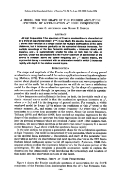
Figure 1. Front view of BRI annex building (left) and
main building (right). These two buildings are connected by
passage ways as seen in the picture.
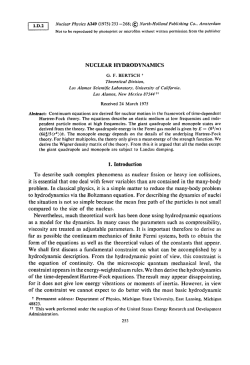
Figure 2. Layout of the seismic observation system in BRI
annex building and in surrounding soil.
time over years. Focus of the paper is also placed on
discussing the cause of the variation.
2
2.1
OUTLINE OF OBSERVATORY BUILDING
AND OBSERVATION SYSTEM
BRI annex building
Continuous earthquake observation has been conducted in Building Research Institute (BRI) of Japan
since 1950s. The BRI annex building is one of the
stations of the BRI strong motion network, and a large
number of earthquake records have been observed with
accelerometers densely installed within the building as
well as in the surrounding soil (Kashima & Kitagawa
2006).
The annex building is a steel-reinforced concrete
framed structure with eight stories above ground and
one story basement, and was completed in 1998. The
external view of this building is shown in Figure 1.
The building is supported by a flat mat foundation
embedded 8.2 m deep in the soil and has no pile. The
annex building is connected to the main building with
passage ways, but the two buildings are separated by
expansion joint and are structurally independent.
2.2
Seismic observation system
Figure 3. Plan of basement floor and location of three
accelerometers installed.
The seismic observation system at BRI site is composed of 22 accelerometers installed in the annex
building, surrounding soil and the main building, and
these are deployed so as to enable to extract the
dynamic characteristics of soil-structure interaction
effects. The configuration of the seismic observation
system is shown in Figure 2. Eleven accelerometers
are installed in the annex building, and seven in the
surrounding soil.
Three accelerometers are installed on both sides of
the basement and top floors, which enables us to evaluate not only translational but also rotational (rocking
and torsional) motions of the system.
Figure 3 shows the plan of the basement floor
and locations of the seismographs. In addition, two
accelerometers are deployed in the east and west sides
of the fifth and second floors. In computing translational motions, floor responses are evaluated by
averaging over the whole records observed on the floor.
Rigid-body rocking motions are evaluated by dividing
the difference of vertical motions at both sides of foundation by the separation distance between the sensors.
In this paper, the effects of torsional motions are not
taken into account.
4
represents the response of the rigid foundation, in
which the components and represent the translational displacement and rocking angle of the foundation, respectively. L denotes a reference length and
superscript T denotes the transpose of a vector. The
matrix [R] = [{1} L−1 {h}] represents a matrix which
relates {uF } to the nodes at which accelerations of the
effective input motions apply, where {1} is a vector
of ones, and {h} = {h(n) , h(n−1) , · · ·, h(1) }T represents
the height of a floor from the bottom of the basement. The vector {uF }, which represents the response
of a foundation during earthquakes and may be interpreted as actual input motions for the superstructure,
is referred to as an effective input motion (Iguchi et al.
2007). The effective input motion differs from the freefield motions because of both kinematic and inertial
interactions.
3.2
The objective of this section is to review briefly the fundamental identification procedure for the continuoustime state-space model including the SSI effects for
preparation for the next section.
The second order differential equation (Equation 1)
may be reduced to the following continuous-time statespace model:
Figure 4. Multi-mass model of a soil-structure system.
2.3
Observed records
More than 560 sets of earthquake records have been
observed in the BRI annex building since the start of
observation in 1998. Among them, the records with
peak ground acceleration (PGA) larger than 10 cm/s2
are selected for analyses. But, somewhat smaller
(PGA > 8 cm/s2 ) records are included when data satisfying the above criteria were not available for more
than a year.As a result, 67 sets of records were analyzed
in this paper.
The peak ground accelerations (PGA) of the
recorded motions are small in general. The largest
PGA of the records is 74 cm/s2 and the largest interstory drift angle was 4.7 × 10−5 rad on the average.
The BRI annex building can be considered not to
have experienced serious structural damage during the
earthquakes.
3
3.1
Modal decomposition in state-space
where
are state and input vectors having 2n elements. And,
METHODOLOGY
is the output vector whose elements represent absolute accelerations of masses. The matrices [Ac ], [Bc ],
[Cc ] and [Dc ] are composed of [M ], [C], [K] and [R].
Subscript c indicates the continuous-time model.
After solving the eigenvalue problem for the system
matrix [Ac ], modal decomposition of Equations 2a and
2b can be achieved as shown by:
Equation of motion for SSI system
In what follows, a formulation of the equation of
motion for a SSI system is developed on the assumption that the superstructure is modeled as n degreesof-freedom shear building supported by a rigid
foundation. Figure 4 shows the analysis model and the
coordinates of the soil-structure system. The equation
of motion for the superstructure may be expressed as
Thus, we have
where [M ], [C], and [K] denote mass, damping, and
stiffness matrices of the superstructure, respectively,
(n) (n−1)
(1)
and {us } = {us , us
, · · · , us }T denotes the relative
displacement vector of the superstructure measured
removing the rigid body motion from the total displacement. In addition, the vector {uF } = { , L }T
where [ c ] is the diagonal matrix composed of eigenvalues λj (j = 1, 2, . . ., 2n), and [ ] is a matrix consisting of the corresponding eigenvector, {ψj }. The
eigenvalues and eigenvectors are given in the form of
n pairs of complex conjugate.
5
The input-output relations of the system will be
given in the image space of the Laplace transform as
shown by:
where {Yc (s)} and {Xc (s)} are the Laplace transform of
{yc } and {xc }, respectively, [Hc (s)] is a transfer function
matrix defined by
where [Vc ] = [Cc ][ ] and [Lc ]T = [ ]−1 [Bc ] represent the mode shape matrix and participation matrix,
respectively. It will be found that the poles of Equation 9 correspond to the eigenvalues of system matrix
[Ac ], and the eigenvalues λj may be expressed as
follows:
Figure 5. Flowchart of the subspace system identification
method for evaluating structural modal parameters. SVD
means singular value decomposition.
where ωj and ξj are the system circular frequency and
damping factor of j-th mode, respectively.
It should be noted that above formulation is valid not
only for the base-fixed system but for the soil-structure
system. If we set as {uF } = { , L }T , then the corresponding results will be those of the base-fixed system.
In case of evaluating the sway-fixed mode, the effective
input motion to the superstructure should be chosen as
{uF } = . The sway-fixed mode may be interpreted as
the soil-structure system which allows only the rigidbody rocking motion of the foundation (Stewart &
Fenves 1998, Todorovska 2009a, b).
3.3
where {xd }k = {xc (k t)} is the observed discrete-time
state vector, [Ad ], [Bd ], [Cd ] and [Dd ] are system
matrices (subscript d denotes discrete-time), and the
subscript k denotes discrete-time step. The system
matrices [Ad ] and [Bd ] for the discrete-time series
will be distinct by comparing with those of the
continuous-time, but these two models are convertible
with each other by using appropriate technique such
as the zero-order-fold assumption. Taking into account
the relation [Ad ] = e[Ac ] t ( t denotes time interval),
the eigenvalue decomposition of the matrix [Ad ] may
be performed in the same manner as Equation 7,
resulting in:
System identification and parameter estimation
Since some advanced system identification methods
are available at present, one can chose an appropriate method applicable to the problem. In this study,
subspace identification method (Conte et al. 2008)
is adopted for identifying dynamic characteristics of
soil-structure system. The subspace method has several advantages; the noticeable one is the capability
for applying to multi-input multi-output system without difficulties. Several algorisms for the subspace
identification have been proposed, and, among those,
the N4SID algorism (Van Overschee et al. 1993)
are applied in this study. It is beyond the scope of
this paper to go deep into the subspace identification
methodology. The detail may be found elsewhere (Van
Overschee & De Moor 1993, Katayama 2005). The
essentials of the subspace identification formulation
will be summarized in what follows.
The discrete-time state-space equations corresponding to Equations 2(a) and (b) can be expressed
as follows.
where [ d ] is a diagonal matrix which consists of the
eigenvalues of [Ad ], µj . From the definition, the relations between the eigenvalues of continuous-time and
discrete-time models may be shown as:
From above equation,
Eigenfrequencies and damping factors of the
continuous-time model can be evaluated by substituting the results obtained by Equation 14 into
Equation 10.
The flowchart of the system identification method
is shown in Figure 5.
6
Figure 7. The relationship between base-fixed frequency
and peak relative velocity (PRV). (a) NS (longitudinal) direction; (b) EW (transverse) direction. The plots are connected
by light lines in chronological order.
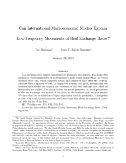
which corresponds to about a 50% reduction in the
rigidity.
The ratio of sway-fixed to base-fixed frequencies,
f˜1 /f1 , are also shown in Figure 6. These results show
that the sway-fixed frequency f˜1 tends to approach to
the base-fixed frequency f1 with a lapse of years in both
directions of the structure. This implies that the effect
of SSI on the fundamental structural frequency has
been relatively decreasing, but does not mean that the
rigidity of soil has changed. The average of the ratio
f˜1 /f1 for all records are 0.98 for NS (longitudinal) and
0.95 for EW (transverse) directions, respectively.
The sway-fixed mode can be decomposed into basefixed and rigid-body-rocking modes, and the swayfixed frequency (f˜1 ) and rocking frequency (fR ) may
be expressed by (Stewart & Fenves 1998, Todorovska
2009a, b):
Figure 6. Variation in base-fixed (f1 ) and sway-fixed (f˜1 ) frequencies. (a) Top: base-fixed ( ; connected by dashed line)
and sway-fixed (◦ ; connected by light solid line) frequencies
for NS (longitudinal) direction. The plotted size implies the
magnitude of peak relative velocities (PRV) of superstructure.
Dashed (base-fixed) and solid (sway-fixed) straight lines represent the regression lines for all plots by the least squares
method. Bottom: ratios of sway-fixed and base-fixed frequencies f˜1 /f1 . (b) Base-fixed and sway-fixed frequencies for EW
(transverse) direction in the same manner as in (a).
4
RESULTS AND DISCUSSION
It should be noted that Equation 16 was derived for a
structure with a flat foundation supported on a soil surface. Though approximate, the equation may be used
for an evaluation of the rigid-body rocking frequency
of a structure with a basement (Todorovska 2009a).
As anticipated from Equation 16, for the case of f˜1 /f1
which is nearly 1, the estimated frequency fR tends to
result in an unstable solution.
As the rocking frequency fR is subjected to the rigidity of the soil, the results will reflect the variation
in soil properties. Though not shown here, the estimated result for fR was found to be almost constant
throughout the observation.The computed rocking frequencies for NS (longitudinal) and EW (transverse)
directions are 7∼8 Hz and 5 Hz, respectively.
Inspecting the results shown in Figure 6, it may be
observed that the fundamental frequency tends to drop
suddenly for relatively large PRVs and to increase in
the next small shaking. The relationship between the
4.1 Variation in base-fixed and sway-fixed
frequencies
The variation in fundamental frequencies for the basefixed mode (f1 ) and the sway-fixed mode (f˜1 ) of the
structure for about ten years is shown in Figure 6.
The transverse axis is the elapsed years from the start
of observation. The plotted results are categorized
into five groups according to the amplitudes of peak
relative velocities (PRV) defined by
We will notice from Figure 6 that base-fixed frequencies f1 have dropped from 1.9 Hz to 1.3 Hz in
about ten years for both longitudinal and transverse
directions. Since there have been no changes in building usage, these results may be attributed mainly to
the degradation of the global stiffness of the structure,
7
Figure 8. The relationship between differences of base-fixed
frequency f1 and the logarithm of peak relative velocity
(PRV). (a) NS (longitudinal) direction; (b) EW (transverse)
direction. Gray thick line represents the regression line and
C.C. indicates the correlation coefficient.
base-fixed frequency f1 and PRV connected in chronological order is shown in Figure 7. The results are
suggesting that there is an obvious relation between the
logarithm of PRV and change in structural frequency
f1 within a short time span. The relationship between
differences in the logarithm of PRV,
Figure 9. Variation in base-fixed and sway-fixed damping
factors. (a) Top: base-fixed ( ; connected by dashed line) and
sway-fixed (◦ ; connected by light line) damping factors for NS
(longitudinal) direction. The plotted sizes implies magnitudes
of peak relative velocities (PRV) of superstructure. Dashed
(base-fixed) and solid (sway-fixed) straight lines represent
regressed results for all plots by the least squares method.
Bottom: ratio of base-fixed and sway-fixed damping factors
ξ˜1 /ξ1 . (b) Base-fixed and sway-fixed damping factors for EW
(transverse) direction in the same manner as in (a).
and the difference of the structural frequencies,
is shown in Figure 8, where superscript (n) indicates
the n-th event. There is almost linear relations between
ln PRV and f1 . Thus, introducing a proportionality
constant , we have a following empirical expression:
the fundamental mode frequencies shown in the previous section. On the average, the damping factor for the
base-fixed system is 3.1% for both directions, and for
the sway-fixed system the damping factors are 2.3%
for NS and 2.6% for EW directions. The ratio of damping factors for these two systems, ξ˜1 /ξ1 , is also shown
in Figure 9.
It should be noted that the damping factors of the
sway-fixed mode (ξ˜1 ) are smaller than the base-fixed
mode (ξ1 ). This tendency may be understood by recalling the relations between ξ1 and ξ˜1 . Damping factors of
sway-fixed system may be approximated by (Stewart
& Fenves 1998):
PRV (n+1)
where RPV =
. The values −1 ln RPV can be
PRV (n)
a measure for estimating the amplitude dependence
of structural frequencies. The estimated proportionality constants are ≈ −15.6 for NS direction and
≈ −17.5 for EW direction. The Equation 19 can be
used to estimate the base-fixed frequency using the
value of RPV .
4.2 Variation in damping factor
The computed results of damping factors for basefixed (ξ1 ) and sway-fixed systems (ξ˜1 ) are shown in
Figure 9. The results of damping factors tend to fluctuate from one earthquake to another, and are showing
somewhat outliers for the events with relatively small
PRVs. This is perhaps the result of lack of resolution
accuracy in the numerical computation. The tendencies about aging and amplitude dependence of the
damping factors can not be detected so clearly as in
where ξR represents the damping factor of the rigidbody rocking mode, which is generally small comparing with ξ1 . In addition, as the ratio f˜1 /fR is smaller than
8
Figure 11. Variation in the fundamental frequencies versus RMS of relative displacement amplitude of superstructure. Black solid and gray broken lines are the results of
base-fixed (structural) and sway-fixed ( system) frequencies,
respectively.
reference (open circles). In the method, the predominant frequency is determined by zero crossing with
positive slope (Clough & Penzien 1993). As the number of zero crossing can be expressed by the spectral
moments in the frequency domain, it may be rewritten
in the form of Equation 22 for the time domain by use
of the Parseval’s theorem. Thus, we have
Figure 10. Variation in the fundamental frequencies during
earthquake motions (EW (transverse) direction). Top: Time
histories of the earthquake ground motions; Middle: Time
histories of base-fixed (structural) frequency (black line) and
sway-fixed (system) frequency (gray line); Bottom: Time histories of root mean square value of the relative displacement
of the superstructure.
f˜1 /f1 the second term of the equation can be omitted.
Eliminating the second term from Equation 20, then
we have:
where T denotes the half width of window, which
was chosen as T = 4 sec . The computation was performed every 4 sec by shifting the time τ along the
time axis. In Figure 10, waveforms of free-field surface accelerations and root mean squares (RMS) of
relative displacements of the superstructure are shown
simultaneously.
Inspection of the results shown in Figure 10 reveals
that both the base-fixed and sway-fixed frequencies tend to decrease with increase in the structural response. The minimal values of frequencies
correspond to the time when the largest structural
response occurred. After that, the frequencies tend to
resume gradually as the structural response becomes
smaller, and the frequencies recover almost to preearthquake values at the end of shaking. Furthermore,
the above mentioned tendencies may be observed
in common for both base-fixed and sway-fixed frequencies. On the other hand, the results obtained by
zero crossing method correspond approximately to the
results obtained by the sophisticated method for large
response amplitudes. However, results by the method
tend to be unreliable for small response amplitudes.
The change in frequency versus structural response
(RMS of relative displacements of superstructure)
is shown in Figure 11. One of the distinct features
detected from the results is that the frequencies are
very much amplitude dependent. It is also interesting
to notice that the variation in frequencies is almost
linear with respect to the logarithm of amplitudes of
Since f˜1 /f1 < 1 as indicated in the previous section, we
have ξ˜1 < ξ1 .
4.3 Variation in frequency during earthquake
It is interesting to study the variation in dynamic
characteristics of soil-structure system not only over
a long period of time but during an earthquake.
Especially the short term change in the frequency is
evidently attributed to strong nonlinearity of structure that might be associated with damage in the
structure. Thus, it becomes important to observe the
frequency change during an earthquake in evaluation
of the seismic-resistance performance of structures.
In this section, we will investigate the change in
base-fixed and sway-fixed frequencies during specific
earthquake motions which have exhibited relatively
large structural responses.
Figure 10 shows the change in frequencies during
three selected earthquakes. The results are numerically evaluated by means of the subspace identification
method introducing a box-type moving window onto
wave forms. In the figure, the frequency change evaluated by the zero crossing method is also plotted for
9
Clough, R. W. & Penzien, J. 1993. Dynamics of structures,
2nd ed., McGraw-Hill.
Conte, J. P., He, X., Moaveni, B., Masri, S. F., Caffrey, J. P.,
Wahbeh, M., Tasbihgoo, F., Whang, D. H. & Elgamal, A.
2008. Dynamic testing of Alfred Zampa memorial bridge,
J. Struct. Eng., ASCE, 134(6), 1006–1016.
Ghanem, R. & Sture, S. (ed.) 2000. Special issue: structural health monitoring, J. Engrg. Mech., ASCE, 126(7),
665–777.
Iguchi, M., Kawashima, M. & Minowa, C. 2007. A measure
to evaluate effective input motions to superstructure, The
4th U.S.-Japan Workshop on Soil-Structure-Interaction,
Tsukuba, Japan.
Kashima, T. & Kitagawa, Y. 2006. Dynamic characteristics
of an 8-storey building estimated from strong motion
records, Proc. of 1st European Conference on Earthquake
Engineering and Seismology, Geneva, Switzerland.
Katayama, T. 2005. Subspace Methods for System Identification, Springer-Verlag, London.
Luco, J. E., Trifunac, M. D. & Wong, H. L. 1987. On the
apparent change in dynamic behavior of nine-story reinforced concrete building, Bull. Seism. Soc. Am. 77(6),
1961–1983.
Stewart, J. P. & Fenves, G. L. 1998. System identification for
evaluating soil-structure interaction effects in buildings
from strong motion recordings, Earthquake Engng. Struct.
Dyn. 27, 869–885.
Todorovska, M. I. & Trifunac, M. D. 2008. Impulse response
analysis of the Van Nuys 7-story hotel during 11 earthquakes and earthquake damage detection, Strut. Control
Health Monit., 15, 90–116.
Todorovska, M. I. 2009a. Seismic interferometry of a soilstructure interaction model with coupled horizontal and
rocking response, Bull. Seism. Soc.Am., 99(2A), 611–625.
Todorovska, M. I. 2009b. Soil-structure system identification of Millikan Library North-South response during four
earthquakes (1970–2002): what caused the observed wandering of the system frequencies?, Bull. Seism. Soc. Am.
99(2A), 626–635.
Trifunac, M. D., Ivanovi´c, S. S. & Todorovska, M. I.
2001a. Apparent periods of a building. I: Fourier analysis,
J. Struct. Eng., ASCE, 127(5), 517–526.
Trifunac, M. D., Ivanovi´c, S. S. & Todorovska, M. I. 2001b.
Apparent periods of a building. II: Time-frequency analysis, J. Struct. Eng., ASCE, 127(5), 527–537.
Van Overschee, P. & De Moor, B. 1993. N4SID: subspace
algorithms for the identification of combined deterministic and stochastic systems, Automatica, 30(1), 75–93.
structural displacement responses. The slopes of the
results shown in Figure 11 have special meaning in
estimating the variation in natural frequency based on
the displacement response of the structure.
5
CONCLUSIONS
The variation in dynamic characteristics of the eightstory steel-reinforced concrete building with the passage of time was investigated based on the earthquake
records observed in the building for about ten years. In
order to evaluate the SSI effects, the dynamic characteristics of the base-fixed and sway-fixed modes were
isolated from the records.
It was revealed that the base-fixed frequency has
decreased from 1.9 Hz to 1.3 Hz in about ten years both
in the longitudinal and transverse directions, which
corresponds to about a 50% reduction in the global
stiffness of the superstructure. On the other hand, the
sway-fixed frequencies were less than the base-fixed
frequencies by 5% in the transverse direction and 2%
in the longitudinal direction, respectively.
With use of the results of the sway-fixed and basefixed frequencies, the frequency of rigid-body rocking
mode was estimated, which showed almost constant
value throughout the observation. These results indicate that the observed variation in frequencies of the
building could be attributed to the stiffness degradation of the superstructure.
Finally, it was shown that the subspace identification method developed by Van Overschee & De Moor
(1993) could be successfully applied to the SSI system.
ACKNOWLEDGEMENT
This research was partially supported by the Ministry
of Education, Culture, Sports, Science and Technology, Grants-in-Aid for Scientific Research (C), Grant
Number 19560580, 2007–2008.
REFERENCES
Clinton, J. F., Bradford, S. C., Heaton, T. H. & Favela, J.
2006. The observed wander of the natural frequencies in
a structure, Bull. Seism. Soc. Am. 96(1), 237–257.
10