
International macroeconomics (advanced level) Lecture notes
International macroeconomics (advanced level) Lecture notes Nikolas A. M¨uller-Plantenberg∗ 2014–2015 ∗ E-mail: [email protected]. Address: Departamento de An´alisis Econ´omico - Teor´ıa Econ´omica e Historia Econ´omica, Universidad Aut´onoma de Madrid, 28049 Cantoblanco, Madrid, Spain. International Macroeconomics CONTENTS Contents I Aims of the course 12 II Basic models 14 1 Balassa-Samuelson effect 14 1.1 Growth accounting . . . . . . . . . . . . . . . . . . . . . . . . . . . . . . . . . . . . . . 14 1.1.1 Example 1 . . . . . . . . . . . . . . . . . . . . . . . . . . . . . . . . . . . . . . 14 1.1.2 Example 2 . . . . . . . . . . . . . . . . . . . . . . . . . . . . . . . . . . . . . . 15 1.1.3 Example 3 . . . . . . . . . . . . . . . . . . . . . . . . . . . . . . . . . . . . . . 15 1.2 The price of non-traded goods with mobile capital . . . . . . . . . . . . . . . . . . . . . 16 1.3 Balassa-Samuelson effect . . . . . . . . . . . . . . . . . . . . . . . . . . . . . . . . . . 20 1.4 Accounting for real exchange rate changes . . . . . . . . . . . . . . . . . . . . . . . . . 22 1.4.1 Theory versus empirics . . . . . . . . . . . . . . . . . . . . . . . . . . . . . . . . 23 31 January 2015 2 International Macroeconomics CONTENTS 1.4.2 Real appreciation of the yen . . . . . . . . . . . . . . . . . . . . . . . . . . . . . 23 1.4.3 Conclusions . . . . . . . . . . . . . . . . . . . . . . . . . . . . . . . . . . . . . . 24 III Difference equations 25 2 Introduction to difference equations 25 2.1 Definition . . . . . . . . . . . . . . . . . . . . . . . . . . . . . . . . . . . . . . . . . . 25 2.2 Examples . . . . . . . . . . . . . . . . . . . . . . . . . . . . . . . . . . . . . . . . . . . 26 2.2.1 Difference equation with trend, seasonal and irregular . . . . . . . . . . . . . . . 26 2.2.2 Random walk . . . . . . . . . . . . . . . . . . . . . . . . . . . . . . . . . . . . . 27 2.2.3 Reduced-form and structural equations . . . . . . . . . . . . . . . . . . . . . . . 28 2.2.4 Error correction . . . . . . . . . . . . . . . . . . . . . . . . . . . . . . . . . . . . 31 2.2.5 General form of difference equation . . . . . . . . . . . . . . . . . . . . . . . . . 32 2.2.6 Solution to a difference equation . . . . . . . . . . . . . . . . . . . . . . . . . . . 33 2.3 Lag operator . . . . . . . . . . . . . . . . . . . . . . . . . . . . . . . . . . . . . . . . . 34 31 January 2015 3 International Macroeconomics CONTENTS 2.4 Solving difference equations by iteration . . . . . . . . . . . . . . . . . . . . . . . . . . 35 2.4.1 Sums of geometric series . . . . . . . . . . . . . . . . . . . . . . . . . . . . . . . 35 2.4.2 Iteration with initial condition - case where |a1| < 1 . . . . . . . . . . . . . . . . . 36 2.4.3 Iteration with initial condition - case where |a1| = 1 . . . . . . . . . . . . . . . . . 37 2.4.4 Iteration without initial condition - case where |a1| < 1 . . . . . . . . . . . . . . . 38 2.4.5 Iteration without initial condition - case where |a1| > 1 . . . . . . . . . . . . . . . 39 2.4.6 The exchange rate as an asset price in the monetary model . . . . . . . . . . . . . 41 2.5 Alternative solution methodology . . . . . . . . . . . . . . . . . . . . . . . . . . . . . . 42 2.5.1 Example: Second-order difference equation . . . . . . . . . . . . . . . . . . . . . 45 2.6 Solving second-order homogeneous difference equations . . . . . . . . . . . . . . . . . . 48 2.6.1 Roots of the general quadratic equation . . . . . . . . . . . . . . . . . . . . . . . 48 2.6.2 Homogeneous solutions . . . . . . . . . . . . . . . . . . . . . . . . . . . . . . . 49 2.6.3 Particular solutions . . . . . . . . . . . . . . . . . . . . . . . . . . . . . . . . . . 54 31 January 2015 4 International Macroeconomics CONTENTS 3 Modelling currency flows using difference equations 55 3.1 A benchmark model . . . . . . . . . . . . . . . . . . . . . . . . . . . . . . . . . . . . . 59 3.2 A model with international debt . . . . . . . . . . . . . . . . . . . . . . . . . . . . . . . 64 IV Differential equations 69 4 Introduction to differential equations 69 5 First-order ordinary differential equations 70 5.1 Deriving the solution to a differential equation . . . . . . . . . . . . . . . . . . . . . . . 71 5.2 Applications . . . . . . . . . . . . . . . . . . . . . . . . . . . . . . . . . . . . . . . . . 73 5.2.1 Inflation . . . . . . . . . . . . . . . . . . . . . . . . . . . . . . . . . . . . . . . . 73 5.2.2 Price of dividend-paying asset . . . . . . . . . . . . . . . . . . . . . . . . . . . . 75 5.2.3 Monetary model of exchange rate . . . . . . . . . . . . . . . . . . . . . . . . . . 76 6 Currency crises 31 January 2015 77 5 International Macroeconomics CONTENTS 6.1 Domestic credit and reserves . . . . . . . . . . . . . . . . . . . . . . . . . . . . . . . . 77 6.2 A model of currency crises . . . . . . . . . . . . . . . . . . . . . . . . . . . . . . . . . 80 6.2.1 Exchange rate dynamics before and after the crisis . . . . . . . . . . . . . . . . . 82 6.2.2 Exhaustion of reserves in the absence of an attack . . . . . . . . . . . . . . . . . . 86 6.2.3 Anticipated speculative attack . . . . . . . . . . . . . . . . . . . . . . . . . . . . 87 6.2.4 Fundamental causes of currency crises . . . . . . . . . . . . . . . . . . . . . . . . 89 7 Systems of differential equations 93 7.1 Uncoupling of differential equations . . . . . . . . . . . . . . . . . . . . . . . . . . . . 93 7.2 Dornbusch model . . . . . . . . . . . . . . . . . . . . . . . . . . . . . . . . . . . . . . 95 7.2.1 The model’s equations . . . . . . . . . . . . . . . . . . . . . . . . . . . . . . . . 95 7.2.2 Long-run characteristics . . . . . . . . . . . . . . . . . . . . . . . . . . . . . . . 96 7.2.3 Short-run dynamics . . . . . . . . . . . . . . . . . . . . . . . . . . . . . . . . . . 96 8 Laplace transforms 100 8.1 Definition of Laplace transforms . . . . . . . . . . . . . . . . . . . . . . . . . . . . . . 100 31 January 2015 6 International Macroeconomics CONTENTS 8.2 Standard Laplace transforms . . . . . . . . . . . . . . . . . . . . . . . . . . . . . . . . . 101 8.3 Properties of Laplace transforms . . . . . . . . . . . . . . . . . . . . . . . . . . . . . . 102 8.3.1 Linearity of the Laplace transform . . . . . . . . . . . . . . . . . . . . . . . . . . 102 8.3.2 First shift theorem . . . . . . . . . . . . . . . . . . . . . . . . . . . . . . . . . . 102 8.3.3 Multiplying and dividing by t . . . . . . . . . . . . . . . . . . . . . . . . . . . . 102 8.3.4 Laplace transforms of the derivatives of f (t) . . . . . . . . . . . . . . . . . . . . 103 8.3.5 Second shift theorem . . . . . . . . . . . . . . . . . . . . . . . . . . . . . . . . . 104 8.4 Solution of differential equations . . . . . . . . . . . . . . . . . . . . . . . . . . . . . . 104 8.4.1 Solving differential equations using Laplace transforms . . . . . . . . . . . . . . . 104 8.4.2 First-order differential equations . . . . . . . . . . . . . . . . . . . . . . . . . . . 105 8.4.3 Second-order differential equations . . . . . . . . . . . . . . . . . . . . . . . . . 106 8.4.4 Systems of differential equations . . . . . . . . . . . . . . . . . . . . . . . . . . . 107 9 The model of section 6.2 revisited 31 January 2015 110 7 International Macroeconomics CONTENTS 10 A model of currency flows in continuous time 112 10.1 The model’s equations . . . . . . . . . . . . . . . . . . . . . . . . . . . . . . . . . . . . 112 10.2 Solving the model as a system of differential equations . . . . . . . . . . . . . . . . . . . 112 10.3 Solving the model as a second-order differential equation . . . . . . . . . . . . . . . . . 114 V Intertemporal optimization 117 11 Methods of intertemporal optimization 117 12 Intertemporal approach to the current account 118 12.1 Current account . . . . . . . . . . . . . . . . . . . . . . . . . . . . . . . . . . . . . . . 118 12.2 A one-good model with representative national residents . . . . . . . . . . . . . . . . . . 119 13 Ordinary maximization by taking derivatives 120 13.1 Two-period model of international borrowing and lending . . . . . . . . . . . . . . . . . 120 13.2 Digression on utility functions . . . . . . . . . . . . . . . . . . . . . . . . . . . . . . . . 123 31 January 2015 8 International Macroeconomics CONTENTS 13.2.1 Logarithmic utility. . . . . . . . . . . . . . . . . . . . . . . . . . . . . . . . . . . 123 13.2.2 Isoelastic utility. . . . . . . . . . . . . . . . . . . . . . . . . . . . . . . . . . . . 125 13.2.3 Linear-quadratic utility. . . . . . . . . . . . . . . . . . . . . . . . . . . . . . . . . 126 13.2.4 Exponential utility. . . . . . . . . . . . . . . . . . . . . . . . . . . . . . . . . . . 127 13.2.5 The HARA class of utility functions . . . . . . . . . . . . . . . . . . . . . . . . . 128 13.3 Two-period model with investment . . . . . . . . . . . . . . . . . . . . . . . . . . . . . 130 13.4 An infinite-horizon model . . . . . . . . . . . . . . . . . . . . . . . . . . . . . . . . . . 133 13.5 Dynamics of the current account . . . . . . . . . . . . . . . . . . . . . . . . . . . . . . 136 13.6 A model with consumer durables . . . . . . . . . . . . . . . . . . . . . . . . . . . . . . 138 13.7 Firms, the labour market and investment . . . . . . . . . . . . . . . . . . . . . . . . . . 142 13.7.1 The consumer’s problem. . . . . . . . . . . . . . . . . . . . . . . . . . . . . . . . 142 13.7.2 The stock market value of the firm. . . . . . . . . . . . . . . . . . . . . . . . . . 144 13.7.3 Firm behaviour. . . . . . . . . . . . . . . . . . . . . . . . . . . . . . . . . . . . . 145 13.8 Investment when capital is costly to install: Tobin’s q 31 January 2015 9 . . . . . . . . . . . . . . . . . . . 146 International Macroeconomics CONTENTS VI Dynamic optimization in continuous time 147 14 Optimal control theory 147 14.1 Deriving the fundamental results using an economic example . . . . . . . . . . . . . . . 147 14.2 The Maximum Principle . . . . . . . . . . . . . . . . . . . . . . . . . . . . . . . . . . . 153 14.3 Standard formulas . . . . . . . . . . . . . . . . . . . . . . . . . . . . . . . . . . . . . . 155 14.4 Literature . . . . . . . . . . . . . . . . . . . . . . . . . . . . . . . . . . . . . . . . . . . 156 31 January 2015 10 International Macroeconomics LIST OF TABLES List of Tables 31 January 2015 11 International Macroeconomics Part I Aims of the course The students of this course follow three different master programmes at the UAM: • Master en Econom´ıa Internacional, • Master en Econom´ıa Cuantitativa, ´ • Master en Globalizaci´on y Pol´ıticas Publicas. This course aims to offer something for all three groups by discussing: • some of the theory and empirics of international macroeconomics, • econometric applications in international macroeconomics, • the challenges for macroeconomic policy in a globalizing world. 31 January 2015 12 International Macroeconomics Methodology Use in international economics Difference equations Differential equations Exchange rate behaviour Hyperinflations Currency crises Example M¨uller-Plantenberg (2006) Cagan (1956) Flood and Garber (1984) M¨uller-Plantenberg (2010) Intertemporal optimization Dynamic general equilibrium Obstfeld and Rogoff (1996) Current account determination Obstfeld and Rogoff (1995) Present value models Current account determination Bergin and Sheffrin (2000) Continuous-time finance Exchange rate behaviour Dumas (1992) Hau and Rey (2006) Blanchard and Quah (1989) Vector autoregressions Real exchange rate behaviour Clarida and Gal´ı (1994) Enders (1988) Cointegration Purchasing power parity Fujii (2006) Error correction models Exchange rate pass-through Nonlinear time series Nonlinear adjustment towards PPP Obstfeld and Taylor (1997) 31 January 2015 13 International Macroeconomics Balassa-Samuelson effect Part II Basic models 1 Balassa-Samuelson effect The Balassa-Samuelson effect is a tendency for countries with higher productivity in tradables compared with nontradables to have higher price levels (Balassa, 1964, Samuelson, 1964). 1.1 Growth accounting Often we can derive relationships between growth rates by • first taking logs of variables, • then differentiating the resulting logarithms with respect to time. 1.1.1 Example 1 z = xy ⇒ log(z) = log(x) + log(y) 31 January 2015 14 International Macroeconomics Balassa-Samuelson effect z˙ x˙ y˙ = + z x y ⇒ zˆ = xˆ + yˆ, ⇒ where the dot above a variable indicates the derivative of that variable with respect to time and the hat above a variable the (continuous) percentage change of that variable. 1.1.2 Example 2 x z= y ⇒ log(z) = log(x) − log(y) z˙ x˙ y˙ ⇒ = − z x y ⇒ zˆ = xˆ − yˆ, 1.1.3 Example 3 z =x+y ⇒ log(z) = log(x + y) 31 January 2015 15 International Macroeconomics Balassa-Samuelson effect z˙ x˙ + y˙ x x˙ y y˙ = = + z x+y zx zy x y ⇒ zˆ = xˆ + yˆ z z ⇒ 1.2 The price of non-traded goods with mobile capital We consider an economy with traded and nontraded goods (p. 199–214, Obstfeld and Rogoff, 1996). We are interested to determine what drives the relative price of nontraded goods, PN . (That is, PN is the price of nontradables in terms of the price of tradables which for simplicity is normalized to unity, pT = 1). We make two important assumptions: • Capital is mobile between sectors and between countries. • Labour is mobile between sectors but not between countries. There are two production functions, one for tradables and one for nontradables, both with constant returns to scale: YT = AT F (KT , LT ), YN = AN G(KN , LN ). 31 January 2015 (1) (2) 16 International Macroeconomics Balassa-Samuelson effect The assumption of constant returns to scale implies that we can work with the production function in intensive form (here, in per capita terms): ( ) YT AT F (KT , LT ) KT yT := = = AT F , 1 = AT F (kT , 1) = AT f (kT ), (3) LT LT LT ( ) YN AN G(KN , LN ) KN (4) yN := = = AN G , 1 = AN G(kN , 1) = AN g(kN ). LN LN LN The marginal products of capital and labour in the tradables sector are therefore: ∂AT LT f (k) 1 = AT LT f ′(k) = AT f ′(k), ∂KT LT ( [ )] ∂AT LT f (k) −K T MPLT := = AT f (k) + LT f ′(k) = AT [f (k) − kf ′(k)] . 2 ∂LT LT MPKT := (5) (6) The marginal products of capital and labour in the nontradables sector are: MPKN = AN g ′(k), MPLN = AN [g(k) − kg ′(k)] . 31 January 2015 (7) (8) 17 International Macroeconomics Balassa-Samuelson effect Suppose now that firms maximize the present value of their profits (measured in units of tradables): )s−t ∞ ( ∑ 1 [AT,sF (KT,s, LT,s) − wsLT,s − (KT,s+1 − KT,s)], (9) 1 + r s=t )s−t ∞ ( ∑ 1 [PN,sAN,sF (KN,s, LN,s) − wsLN,s − (KN,s+1 − KN,s)]. (10) 1 + r s=t Profit maximization yields four equations with four unknowns (w, PN , kT , kN ): MPKT MPLT MPKN MPLN = AT f ′(kT ) = r, = AT [f (kT ) − f ′(kT )kT ] = w, = PN AN g ′(kN ) = r, = PN AN [g(kN ) − g ′(kN )kN ] = w. (11) (12) (13) (14) By combining equations (11) and (12) as well as equations (13) and (14), we find that the per capita products in both sectors are equal to the per capita cost of the factor inputs: AT f (kT ) = rkT + w, PN AN g(kN ) = rkN + w. 31 January 2015 (15) (16) 18 International Macroeconomics Balassa-Samuelson effect Equations (15) and (16) just represent Euler’s theorem for the constant-returns-to-scale production function (in this case, in per capita terms). Both equations become more tractable once we take logs and differentiate with respect to time. We start with equation (15): log(AT ) + log(f (kT )) = log(rkT + w) A˙ T f ′(kT )k˙ T rk˙ T + w˙ rk˙ T + w˙ ⇒ + = = AT f (kT ) rkT + w AT f (kT ) rkT ˆ rkT ˆ w ⇒ AˆT + kT = kT + wˆ AT f (kT ) AT f (kT ) AT f (kT ) ⇒ AˆT = µLT w, ˆ (17) (18) (19) (20) where w . AT f (kT ) Note that we assume that the interest rate is constant. For equation (16) we get a similar result: µLT := (21) PˆN + AˆN = µLN w, ˆ (22) where µLN := 31 January 2015 w . AN g(kN ) (23) 19 International Macroeconomics Balassa-Samuelson effect As seems intuitive, wages in the traded and nontraded goods sectors are determined by the productivity growth rates and wage shares in both sectors. By combining the last two results, we find that the relative price of nontradables grows according to the following equation: µLN ˆ PˆN = AT − AˆN . (24) µLT Note that it is plausible to assume that the production of nontradables is relatively labour-intensive: µLN ≥ 1. (25) µLT 1.3 Balassa-Samuelson effect We assume there are two countries: • Traded goods have the same price at home and abroad (equal to unity). • Nontraded goods have distinct prices at home and abroad, PN and PN∗ . We suppose further that the domestic and foreign price levels are geometric averages of the prices of tradables and nontradables: P = PTγ PN1−γ = PN1−γ , P ∗ = (PT∗ )γ (PN∗ )1−γ = (PN∗ )1−γ . 31 January 2015 (26) (27) 20 International Macroeconomics Balassa-Samuelson effect The real exchange rate thus depends only on the relative prices of nontradables: ( )1−γ P PN Q= ∗ = P PN∗ (28) To see how the inflation rates differ in both countries, we can log-differentiate this ratio: Pˆ − Pˆ ∗ = (1 − γ)(PˆN − PˆN∗ ) ] [ µLN ˆ (AT − Aˆ∗T ) − (AˆN − Aˆ∗N ) = (1 − γ) µ [(LT ) ( )] µLN ˆ µ LN = (1 − γ) AT − AˆN − Aˆ∗T − Aˆ∗N µLT µLT (29) The country with the higher productivity growth in tradables compared with nontradables experiences a real appreciation over time (for example, Japan versus the United States in the second half of the twentieth century). The reasoning here can also explain why rich countries tend to have higher price levels: • Rich countries have become rich due to higher productivity growth. • In general, productivity growth in rich countries has been particularly high in the tradables sector compared with nontradables sector. 31 January 2015 21 International Macroeconomics Balassa-Samuelson effect 1.4 Accounting for real exchange rate changes Let us now turn to the question how the prices of nontraded goods affect the real exchange rate at different horizons. First, we express the real exchange rate in terms of tradables and nontradables prices (all in logarithms): q = s + p − p∗ = s + γ(pT − p∗T ) + (1 − γ)(pN − p∗N ) = s + (pT − p∗T ) + (1 − γ) [(pN − pT ) − (p∗N − p∗T )] = x + y, (30) where x = s + (pT − p∗T ), y = (1 − γ) [(pN − pT ) − (p∗N − p∗T )] . Differentiation with respect to time yields: qˆ = xˆ = sˆ + (ˆ pT − pˆ∗T ) 31 January 2015 + yˆ + (1 − γ) [(ˆ pN − pˆT ) − (ˆ p∗N − pˆ∗T )] . 22 (31) (32) International Macroeconomics Balassa-Samuelson effect 1.4.1 Theory versus empirics • According to the Balassa-Samuelson hypothesis, most of the changes in the real exchange rate at long horizons are accounted for by differences in the relative prices of nontradable goods, y. • Similarly, most of the recent literature on real exchange rates emphasizes movements in the nontraded-goods component, y. • However, Engel (1999) has shown empirically that the nontraded-goods component, y, has accounted for little of the movement in real exchange rates [...] at any horizon: While I cannot be very confident about my findings at longer horizons, knowledge of the behaviour of the relative price on nontraded goods contributes practically nothing to one’s understanding of [...] real exchange rates. 1.4.2 Real appreciation of the yen Engel (1999) discusses whether the real appreciation of the yen over recent decades can be accounted for by changes in the relative prices of nontradables: • Nontraded-goods prices have risen steadily relative to traded-goods prices in Japan since 1970; at the same time, the yen has, consistent with the theory, appreciated considerably in real terms. 31 January 2015 23 International Macroeconomics Balassa-Samuelson effect • However, the rise in nontraded-goods prices may not be responsible for the rise of the yen after all: – First, the increase in the relative price of nontraded goods in Japan was about 40%, whereas the real exchange rate appreciated around 90%. – Second, the relative price of nontradables rose rather monotonously, yet there were periods of strong depreciation of the yen. – Finally, the relative price of nontradables rose elsewhere as well, reducing the size of y. For instance, the relative price of nontradables in the United States has closely mirrored the relative price of nontradables in Japan. 1.4.3 Conclusions • At long horizons, the Balassa-Samuelson hypothesis may be valid and differences in relative prices may be responsible for movements in the real exchange rate. • At least at short and medium horizons, however, it is the difference of tradable-goods prices that is mainly responsible for the movements of the real exchange rate. • It is quite possible that changes in the real exchange rate stem primarily from changes in the nominal exchange rates, even at rather long horizons. 31 January 2015 24 International Macroeconomics Introduction to difference equations Part III Difference equations 2 Introduction to difference equations Much of economic analysis, particularly in macroeconomics, nowadays centers on the analysis of time series. Time series analysis: • Time series analysis is concerned with the estimation of difference equations containing stochastic components. 2.1 Definition Difference equations express the value of a variable in terms of: • its own lagged values, • time and other variables. 31 January 2015 25 International Macroeconomics Introduction to difference equations 2.2 Examples 2.2.1 Difference equation with trend, seasonal and irregular y t = Tt + S t + I t Tt = 1 + 0, 1t (π ) St = 1, 6 sin t 6 It = 0, 7It−1 + εt Equation (33) is a difference equation. 31 January 2015 26 observed variables, trend, (33) (34) seasonal, (35) irregular. (36) International Macroeconomics Introduction to difference equations 2.2.2 Random walk Stock price modelled as random walk: yt+1 = yt + εt+1, where yt = stock price, εt+1 = random disturbance. Test: ∆yt+1 = α0 + α1yt + εt+1. H0: α0 = 0, α1 = 0. H1: otherwise. 31 January 2015 27 International Macroeconomics Introduction to difference equations 2.2.3 Reduced-form and structural equations Samuelson’s (1939) classic model: y t = c t + it , ct = αyt−1 + εc,t, it = β(ct − ct−1) + εi,t, 0 < α < 1, β > 0, (37) (38) (39) where yt := real GDP, ct := consumption, it := investment, εc,t ∼ (0, σc2), εi,t ∼ (0, σi2). 31 January 2015 (40) 28 International Macroeconomics Introduction to difference equations Structural equation A structural equation expresses an endogenous variable in terms of: • the current realization of another endogenous variable (among other variables) Reduced-form equation A reduced-form equation is one expressing the value of a variable in terms of: • its own lags, • lags of other endogenous variables, • current and past values of exogenous variables, • disturbance terms. 31 January 2015 29 International Macroeconomics Introduction to difference equations Therefore, • equation (37) is a structural equation, • equation (38) is a reduced-form equation, • equation (39) is a structural equation, Equation (39) in reduced form: it = αβ(yt−1 − yt−2) + β(εc,t − εc,t−1) + εi,t. (41) Equation (39) in univariate reduced form: yt = α(1 + β)yt−1 − αβyt−2 + (1 + β)εc,t − βεc,t−1 + εi,t. 31 January 2015 30 (42) International Macroeconomics Introduction to difference equations 2.2.4 Error correction The Unbiased Forward Rate (UFR) hypothesis asserts: st+1 = ft + εt+1 (43) with Et(εt+1) = 0, (44) where ft = forward exchange rate. (45) We can test the UFR hypothesis as follows: st+1 = α0 + α1ft + εt+1, H0 : H1 : α0 = 0, α1 = 1, otherwise. (46) Et(εt+1) = 0, (47) Adjustment process: st+2 = st+1 − α(st+1 − ft) + εs,t+2, ft+1 = ft + β(st+1 − ft) + εf,t+1, 31 January 2015 α > 0, β > 0. 31 (48) (49) International Macroeconomics Introduction to difference equations 2.2.5 General form of difference equation An nth-order difference equation with constant coefficients can be written as follows: yt = α0 + n ∑ αiyt−i + xt, (50) i=1 where xt is a forcing process, which can be a function of: • time, • current and lagged values of other variables, • stochastic disturbances. 31 January 2015 32 International Macroeconomics Introduction to difference equations 2.2.6 Solution to a difference equation The solution to a difference equation is a function of: • elements of the forcing process xt, • time t, • initial conditions (given elements of the y sequence). Example: yt = yt−1 + 2, yt = 2t + c, 31 January 2015 difference equation, solution. 33 (51) (52) International Macroeconomics Introduction to difference equations 2.3 Lag operator The lag operator L (backshift operator) is defined as follows: Liyt = yt−i, i = 0, ±1, ±2, . . . (53) Some implications: Lc = c, where c is a constant, (Li + Lj )yt = Liyt + Lj yt = yt−i + yt−j , LiLj yt = Liyt−j = yt−i−j , LiLj yt = Li+j yt = yt−i−j , L−iyt = yt+i. 31 January 2015 (54) (55) (56) (57) (58) 34 International Macroeconomics Introduction to difference equations 2.4 Solving difference equations by iteration 2.4.1 Sums of geometric series Note that when |k| < 1, m ∑ i=0 1 − k m+1 k = 1−k i and ∞ ∑ ki = i=0 1 , 1−k (59) since 1 − k m+1 1 + k + k + ... + k = 1−k 2 ⇔ (1 − k)(1 + k + k + . . . + k m) = 1 + k − k + k 2 − k 2 + . . . + k m − k m + k m+1 = 1 − k m+1. 2 m (60) (61) Note that when |k| > 1, m ∑ k −i i=0 31 January 2015 −k + k −m = 1−k and ∞ ∑ i=0 k −i = −k , 1−k 35 (62) International Macroeconomics since m ∑ k −i i=0 = m ∑ ( i=0 k Introduction to difference equations ) −1 i ( ) −1 m+1 1− k = 1 − (k −1) k − k −m −k + k −m = = . k−1 1−k (63) 2.4.2 Iteration with initial condition - case where |a1| < 1 Consider the first-order linear difference equation: yt = a0 + a1yt−1 + xt. (64) Iterating forward, using a given initial condition: y1 = a0 + a1 y0 + x1 y2 = a0 + a1 y1 + x2 = a0 + a1(a0 + a1y0 + x1) + x2 = a0 + a0a1 + a21y0 + a1x1 + x2 ... t−1 t−1 ∑ ∑ yt = a0 ai1 + at1y0 + ai1xt−i. i=0 31 January 2015 (65) i=0 36 International Macroeconomics Introduction to difference equations 2.4.3 Iteration with initial condition - case where |a1| = 1 What if |a| = 1? yt = a0 + yt−1 + xt ⇔ ∆yt = a0 + xt. (66) Iterate forward: y1 = a0 + y0 + x1 y2 = a0 + y1 + x2 = a0 + a0 + a1 y0 + x1 + x2 = a0 + a0 + y0 + x1 + x2 ... t ∑ yt = a0 t + y0 + xt−i. (67) i=1 31 January 2015 37 International Macroeconomics Introduction to difference equations 2.4.4 Iteration without initial condition - case where |a1| < 1 Iterating backward: yt = a0 + a1yt−1 + xt = a0 + a1(a0 + a1yt−2 + xt−1) + xt = a0 + a0a1 + a21yt−2 + xt + a1xt−1 = ... m m ∑ ∑ = a0 ai1 + am+1 yt−m−1 + ai1xt−i. 1 i=0 (68) i=0 If |a1| < 1, we therefore obtain the following solution: ∑ 1 − am+1 1 m+1 + a1 yt−m−1 + ai1xt−i, yt = a0 1 − a1 i=0 m (69) which in the limit simplifies to: ∞ ∑ a0 yt = + ai1xt−i. 1 − a1 i=0 31 January 2015 (70) 38 International Macroeconomics Introduction to difference equations A more general solution: ∞ ∑ a0 t yt = Aa1 + + ai1xt−i. 1 − a1 i=0 (71) 2.4.5 Iteration without initial condition - case where |a1| > 1 To obtain a converging solution when |a1| > 1, it is necessary to invert equation (64) and to iterate it forward: yt = a0 + a1yt−1 + xt a0 1 1 ⇔ yt = − + yt+1 − xt+1 a1 a1 a1 ) ( )m+1 ( m ( )i+1 m i ∑ ∑ a0 1 1 1 =− + yt+m+1 − xt+i+1 a1 i=0 a1 a1 a 1 i=0 ( )m+1 m ( )i+1 ∑ a0 −a1 + a−m 1 1 1 yt+m+1 − xt+i+1 =− + a1 1 − a1 a1 a 1 i=0 31 January 2015 39 (72) (73) International Macroeconomics Introduction to difference equations As m approaches infinity, this ”forward-looking” solution converges (unless yt or xt grow very fast): ∞ ( )i+1 ∑ a0 1 yt = − xt+i+1 (74) 1 − a1 i=0 a1 We may write this more compactly as follows: yt = a˜0 + a˜1yt+1 + ˜bxt+1 m m ∑ ∑ i m+1 = a˜0 a˜1 + a˜ yt+m+1 + ˜b a˜i1xt+i+1 i=0 ∞ ∑ a˜0 ˜ a˜i1xt+i+1, +b = 1 − a˜1 i=0 (75) i=0 where a˜0 = − a0 , a1 a˜1 = 1 , a1 ˜b = − 1 . a1 An important drawback of iterative method is that the algebra becomes very complex in higher-order equations. 31 January 2015 40 International Macroeconomics Introduction to difference equations 2.4.6 The exchange rate as an asset price in the monetary model In the monetary model with flexible prices, the current exchange rate, st, depends on the expected future exchange rate, set. Rational expectations imply that agents’ expectations coincide with realized values of the exchange rate, that is, set = st+1. The equation determining today’s nominal exchange rate then becomes: st = a˜1st+1 + ˜bft (76) where b ˜b = 1 , , ft = −(mt − m∗t ) + a(yt − yt∗) + qt. 1+b 1+b The solution to this difference equation is: a˜1 = st = ˜b ∞ ∑ a˜i1ft+i. (77) i=0 Today’s exchange rate thus depends, just like an asset price, on its current and future fundamentals. 31 January 2015 41 International Macroeconomics Introduction to difference equations 2.5 Alternative solution methodology Consider again the first-order linear difference equation (64): yt = a0 + a1yt−1 + xt. (78) Homogeneous part of equation (64): yt − a1yt−1 = 0. (79) Homogeneous solution. A solution to equation (79) is called homogeneous solution, yth. Particular solution. A solution to equation (64) is called particular solution, ytp. 31 January 2015 42 International Macroeconomics Introduction to difference equations General solution. The general solution to a difference equation is defined to be a particular solution plus all homogeneous solutions: yt = yth + ytp. (80) In the case of equation (64): yth = Aat1, (81) where A is an arbitrary constant. Using this homogeneous solution, the homogeneous part of equation (64) is satisfied: = 0. Aat1 − a1Aat−1 1 (82) We already found a particular solution to equation (64): ∞ ytp ∑ a0 = + ai1xt−i 1 − a1 i=0 31 January 2015 for |a1| < 1. (83) 43 International Macroeconomics Introduction to difference equations Therefore the general solution is: yt = yth + ytp = Aat1 ∞ ∑ a0 + + ai1xt−i. 1 − a1 i=0 (84) When initial conditions are given, the arbitrary constant A can be eliminated. Solution methodology: Step 1. Find all n homogeneous solutions. Step 2. Find a particular solution. 31 January 2015 44 International Macroeconomics Introduction to difference equations Step 3. Obtain general solution (= sum of particular solution and linear combination of all homogeneous solutions). Step 4. Eliminate arbitrary constants by imposing initial conditions. 2.5.1 Example: Second-order difference equation Consider the following second-order difference equation (n = 2): 3 . 0.2 yt−2 + |{z} yt = |{z} 0.9 yt−1 − |{z} a1 a2 (85) a0 Homogeneous part: yt − 0.9yt−1 + 0.2yt−2 = 0 31 January 2015 (86) 45 International Macroeconomics Introduction to difference equations Step 1. There are two homogeneous solutions (check!): h y1t = 0.5t, (87) h y2t = 0.4t. Step 2. There is for example the following particular solution (check!): ytp = 10. (88) Step 3. Now we form the general solution: yt = A10.5t + A20.4t + 10. 31 January 2015 (89) 46 International Macroeconomics Introduction to difference equations Step 4. Suppose there are the following initial conditions: y0 = 13, y1 = 11.3 ⇔ A1 = 1, A2 = 2. (90) The solution with initial conditions imposed is thus: yt = 0.5t + 0.4t + 10. (91) Remaining problems: • How do we find homogeneous solutions to a given difference equation? • How do we find a particular solution to a given difference equation? 31 January 2015 47 International Macroeconomics Introduction to difference equations 2.6 Solving second-order homogeneous difference equations 2.6.1 Roots of the general quadratic equation A quadratic equation of the form ax2 + bx + c = 0 (92) has the following solution: √ √ 2 −b ± b − 4ac −b ± d x1,2 = = . 2a 2a (93) When a = 1, the quadratic equation becomes: x2 + bx + c = 0 (94) The above solution simplifies to: √ √ 2 −b ± b − 4c −b ± d = . x1,2 = 2 2 (95) Note that d is called the discriminant. 31 January 2015 48 International Macroeconomics Introduction to difference equations 2.6.2 Homogeneous solutions Consider the homogeneous part of a second-order linear difference equation: yt − a1yt−1 − a2yt−2 = 0. (96) We try yth = Aαt as a homogeneous solution: Aαt − a1Aαt−1 − a2Aαt−2 = 0. (97) Note that the choice of A is arbitrary. Now divide by Aαt−2: α2 − a1α − a2 = 0. (98) This equation is called the characteristic equation. The roots (= solutions) of this equation are called characteristic roots. The characteristic equation of the second-order linear difference equation has the following solutions: √ √ a1 ± a21 + 4a2 a1 ± d α1,2 = = , (99) 2 2 where d (= a21 + 4a2) is the discriminant. 31 January 2015 49 International Macroeconomics Introduction to difference equations We obtain the following solution for the homogeneous equation: yth = A1α1t + A2α2t . (100) To see why this is the solution, just substitute equation (100) into equation (96): ) ( ) ( t t t−1 t−1 t−2 t−2 − a2 A1α1 + A2α2 =0 A1α1 + A2α2 − a1 A1α1 + A2α2 ( t ) ( ) ⇔ A1 α1 − a1α1t−1 − a2α1t−2 + A2 α2t − a1α2t−1 − a2α2t−2 = 0 ( ) ( ) ⇔ A1 α12 − a1α11 − a2 + A2 α22 − a1α21 − a2 = 0. (101) (102) (103) We call α1 and α2 the characteristic roots of equation (96) since they are the roots of the characteristic equation (98). Note that it is sometimes possible to guess the roots of the characteristic equation: (α − α1)(α − α2) = 0 ⇔ α2 − (α1 + α2)α + α1α2 = 0. (104) (105) Therefore the coefficients a1 and a2 are related to the characteristic roots α1 and α2 as follows: a1 = α1 + α2, a2 = −α1α2. 31 January 2015 (106) 50 International Macroeconomics Introduction to difference equations Consider for example the following equation: α2 − 0.5α + 0.06 = 0. (107) This equation has the roots α1 = 0.2 and α2 = 0.3, (108) a1 = 0.2 + 0.3 = 0.5, a2 = −0.2 × 0.3 = −0.06. (109) since Depending on the value of d, we have to distinguish three cases: Case where d > 0. • The characteristic roots in this case are: √ a1 ± d α1,2 = . 2 (110) • The characteristic roots are real and distinct. 31 January 2015 51 International Macroeconomics Introduction to difference equations • The homogeneous solution is: yth = A1α1t + A2α2t . (111) • yt is stable if |α1| < 1 and |α2| < 1. Case where d = 0. • The characteristic roots in this case are: a1 α1 = α2 = α = . 2 (112) • The characteristic roots are real and equal. • The homogeneous solution is: yth = A1αt + A2tαt. (113) • yt is stable if |α| < 1. 31 January 2015 52 International Macroeconomics Introduction to difference equations Case where d < 0. • The characteristic roots in this case are: √ α1 ± i d α1,2 = . 2 (114) • The characteristic roots are imaginary and distinct. • The homogeneous solution is: yth = β1rt cos(θt + β2) (115) where β1,2 = arbitrary constants, √ r = −a2, (a ) 1 θ = arccos . 2r (116) • yt is stable if r < 1. 31 January 2015 53 International Macroeconomics Introduction to difference equations 2.6.3 Particular solutions Let us now turn to the question of how to find a particular solution to a second-order linear difference equation: yt − a1yt−1 − a2yt−2 = ct. (117) In a number of important cases, there are functions that are known to work as particular solutions. Here are some examples: ct ct ct ct ct =c = ct + d = tn = ct = α sin(ct) + β cos(ct) ytp ytp ytp ytp ytp = A, = At + B, = A 0 + A 1 t + . . . + A n tn , = Act, = A sin(ct) + B cos(ct), The constants can be determined by the method of undetermined coefficients: • Substitute the solution (118) into equation (117). • Determine the constant A and B in terms of the other constants. 31 January 2015 54 (118a) (118b) (118c) (118d) (118e) International Macroeconomics Modelling currency flows using difference equations 3 Modelling currency flows using difference equations See M¨uller-Plantenberg (2006). The basic idea is conveyed in the diagram. 31 January 2015 55 International Macroeconomics Modelling currency flows using difference equations Current account Real exchange rate Cash flow (unobserved) Foreign exchange market Debt balance Balance of payments Cash flow and exchange rate determination. 31 January 2015 56 Nominal exchange rate International Macroeconomics 25 Modelling currency flows using difference equations JAPAN 25 0 1990 2000 ITALY 1990 2000 KOREA 2000 EURO AREA 25 1990 2000 FRANCE 1990 2000 CANADA 0 1990 2000 NETHERLANDS 1990 2000 2000 1990 2000 UNITED KINGDOM 0 1980 1990 2000 Large current account surpluses. 31 January 2015 1990 NORWAY 1980 25 0 1980 2000 0 1980 25 1990 RUSSIA 1980 25 0 1980 1980 0 1980 25 0 25 1990 0 1980 UNITED STATES 0 1980 25 0 25 25 0 1980 25 GERMANY 57 1980 1990 2000 International Macroeconomics Modelling currency flows using difference equations 17.5 15.0 Current account Nominal effective exchange rate Nominal effective exchange rate (counterfactual) 4.6 4.4 12.5 10.0 4.2 7.5 4.0 5.0 3.8 2.5 3.6 0.0 −2.5 3.4 1970 1975 1980 1985 1990 1995 Japanese current account and counterfactual exchange rate. 31 January 2015 58 2000 International Macroeconomics Modelling currency flows using difference equations 3.1 A benchmark model The benchmark model consists of the following equations: st = −ξct, qt = st, zt + ct = 0, zt = zt−1 − ϕqt−1, (119) (120) (121) (122) where qt st zt ct ϕ, ξ = real exchange rate, = nominal exchange rate, = current account, = monetary account (= minus country’s cash flow), > 0. Whereas the parameter ϕ measures the exchange rate sensitivity of trade flows, the parameter ξ determines how the nominal exchange rate is affected by a country’s international cash flow, ct. Transform model into first-order difference equation in the current account variable, zt: zt = (1 − ϕξ)zt−1. 31 January 2015 59 International Macroeconomics Modelling currency flows using difference equations The solution to this equation is: zt = A(1 − ϕξ)t, where A is an arbitrary constant. Now the solution for st, qt and ct can be derived from the model’s equations. We make the following observations: • When ϕξ > 1, the current account and all the other variables in the model start to oscillate from one period to the next. • As soon as ϕξ > 2, the model’s dynamic behaviour becomes explosive. • The current account, zt, and the real exchange rate, qt, are positively correlated. 31 January 2015 60 International Macroeconomics 30 Modelling currency flows using difference equations Current account Debt securities balance 20 10 0 −10 −20 1980 1985 1990 1995 Current account and lending in Japan. 31 January 2015 61 2000 International Macroeconomics Modelling currency flows using difference equations Current account (percentage of world trade) 0.5 0.0 1980 1985 1990 1995 2000 1990 1995 2000 1995 2000 5.00 4.75 4.50 Real effective exchange rate 1980 1985 −6.5 −7.0 US−Korean bilateral exchange rate (USD/KRW) 1980 1985 1990 Korea’s current account and exchange rate. 31 January 2015 62 International Macroeconomics Japan Modelling currency flows using difference equations Industrial countries All countries 1.0 0.8 0.6 0.4 0.2 1960 1965 1970 1975 1980 1985 1990 Japan’s share of world reserves. 31 January 2015 63 1995 2000 International Macroeconomics Modelling currency flows using difference equations 3.2 A model with international debt We have so far assumed that countries pay for their external transactions immediately. We shall now make the more realistic assumption that countries finance their external deficits by borrowing from abroad. Specifically, they use debt with a one-period maturity to finance their international transactions. Another assumption we adopt is that debt flows are merely accommodating current account imbalances, that is, we exclude independently fluctuating, autonomous capital flows from our analysis. The previous model is modified as follows: st = −ξct, qt = st, zt + dt + ct = 0, dt := d1t − d1t−1, ct = d1t−1, zt = zt−1 − ϕqt−1, 31 January 2015 (123) (124) (125) (126) (127) (128) 64 International Macroeconomics Modelling currency flows using difference equations where dt := debt balance (part of financial account of the balance of payments), d1t := flow of foreign debt with a one-period maturity, created in period t. (129) Observe that equations (125), (126) and (127) imply that countries pay for their imports and receive payments for their exports always after one period: ct = −zt−1. (130) Due to the deferred payments, adjustments now take longer than in the previous model. The model can be reduced to a second-order difference equation in the current account variable, zt: zt = zt−1 − ϕξzt−2. (131) As long as ϕξ > 41 , the solution to this equation is the following trigonometric function: zt = B1rt cos(θt + B2), where √ r := ϕξ, θ := arccos ( 1 √ 2 ϕξ (132) ) (133) , θϵ[0, π]. 31 January 2015 65 International Macroeconomics Modelling currency flows using difference equations We make the following observations: • As in the previous model, the variables move in a cyclical fashion. However, oscillating behaviour occurs already when ϕξ > 14 (before, the condition was that ϕξ > 1). • Whereas the frequency of the cycles, say ω, was one-half in the previous model—the variables were oscillating from one period to the next, completing one cycle in two periods—in this model ω is strictly less than one-half. • The present model becomes unstable as soon as ϕξ > 1. In the previous model, the corresponding condition was that product of the parameters had to be greater than two, ϕξ > 2. In other words, balance of payments and exchange rate fluctuations are potentially less stable when countries borrow from, and lend to, each other. With international borrowing and lending, exchange rate adjustment is slower, implying that balance of payments imbalances can grow larger. • The correlation between the current account and the exchange rate is still positive; however, the exchange rate now lags the movements of the current account. 31 January 2015 66 International Macroeconomics Modelling currency flows using difference equations Benchmark model Oscillating behaviour ϕξ > 1 Frequency of cycles ω= Explosive behaviour ϕξ > 2 1 2 Model with debt ϕξ > ω< 1 4 1 2 ϕξ > 1 Correlation between z and s Corr(zt, st) = +1 Corr(zt, st+1) = +1 since z1 = 1ξ st 31 January 2015 67 since z1 = 1ξ st+1 International Macroeconomics Modelling currency flows using difference equations Remarks: • The period of the cycles in equation (132), p is: p := 2π . θ (134) • The frequency of the cycles in equation (132), ω, is: ω := 1 θ = . p 2π (135) • Since for there to be cycles in zt, 14 < ϕξ < ∞, we know that 0 < θ < π. From there we get the result regarding the frequency of the cycles: 1 0<ω< . 2 31 January 2015 (136) 68 International Macroeconomics Introduction to differential equations Part IV Differential equations 4 Introduction to differential equations Instead of using difference equations, it is sometimes more convenient to study economic models in continuous time using differential equations. Definition: • A differential equation is a mathematical equation for an unknown function of one or several variables that relates the values of the function itself and of its derivatives of various orders. 31 January 2015 69 International Macroeconomics First-order ordinary differential equations 5 First-order ordinary differential equations We denote the first and second derivative of a variable x with respect to time t as follows: dx x˙ := , dt d2 x x¨ := 2 . dt (137) What is a differential equation? • In a differential equation, the unknown is a function, not a number. • The equation includes one or more derivatives of the function. The highest derivative of the function included in a differential equation is called its order. Further, we distinguish ordinary and partial differential equations: • An ordinary differential equation is one for which the unknown is a function of only one variable. In our case, that variable will be time. • Partial differential equations are equations where the unknown is a function of two or more variables, and one or more of the partial derivatives of the function are included. 31 January 2015 70 International Macroeconomics First-order ordinary differential equations 5.1 Deriving the solution to a differential equation Consider the first-order differential equation: x(t) ˙ = ax(t) + b(t), (138) The function b(t) is called ”forcing function”. We can derive a solution as follows: x(t) ˙ − ax(t) = b(t) −at ⇔ x(t)e ˙ − ax(t)e−at = b(t)e−at ] d [ ⇔ x(t)e−at = b(t)e−at. dt Note that the term e−at is called the ”integrating factor”. For t2 > t1, we obtain: ∫ t2 x(t2)e−at2 − x(t1)e−at1 = b(u)e−audu t1 ∫ t2 ⇔ x(t2) = x(t1)ea(t2−t1) + b(u)e−a(u−t2)du t1 ∫ t2 ⇔ x(t1) = x(t2)e−a(t2−t1) − b(u)e−a(u−t1)du. t1 31 January 2015 71 (139) (140) (141) (142) (143) (144) International Macroeconomics First-order ordinary differential equations (145) Case where a < 0. In this case, as t1 → −∞: ∫ t2 x(t2) → b(u)ea(t2−u)du −∞ ∫ t or x(t) → b(u)ea(t−u)du. (146) (147) −∞ Case where a > 0. In this case, as t2 → ∞: ∫ ∞ x(t1) → − b(u)e−a(u−t1)du t1 ∫ ∞ or x(t) → − b(u)e−a(u−t)du. (148) (149) t 31 January 2015 72 International Macroeconomics First-order ordinary differential equations 5.2 Applications 5.2.1 Inflation Suppose that inflation increases whenever money growth falls short of current inflation: π(t) ˙ = a (π(t) − µ(t)) , (150) where π(t) = inflation, µ(t) = money growth, a > 0. (151) We can solve for π(t): π(t) ˙ = aπ(t) + b(t), (152) where b(t) = −aµ(t). 31 January 2015 (153) 73 International Macroeconomics First-order ordinary differential equations Then current inflation is determined by future money growth: ∫ ∞ π(t) = − b(u)e−a(u−t)du ∫ t∞ =a µ(u)e−a(u−t)du. t 31 January 2015 74 (154) International Macroeconomics First-order ordinary differential equations 5.2.2 Price of dividend-paying asset Consider the following condition which equalizes the returns on an interest-bearing and a dividendpaying asset: R= ⇔ ˙ π(t) q(t) + q(t) q(t) q(t) ˙ = Rq(t) − π(t), (155) (156) where R = interest rate (constant), q(t) = price of dividend-paying asset, π(t) = dividend. (157) The condition implies that the current price of the dividend-paying asset depends on the present discounted value of all future dividends: ∫ ∞ q(t) = π(u)e−R(u−t)du. (158) t 31 January 2015 75 International Macroeconomics First-order ordinary differential equations 5.2.3 Monetary model of exchange rate Consider a continuous-time version of the monetary model of exchange rate determination: m(t) − p(t) = ay(t) − bR(t), q(t) = p(t) − p∗(t) + s(t), R(t) = R∗(t) − s(t). ˙ (159) (160) (161) The model can be rewritten in terms of an ordinary differential equation of the nominal exchange rate variable (for simplicity without the time argument): s˙ = R∗ − R 1 = [(m − m∗) − (p − p∗) − a(y − y ∗)] b (162) 1 ∗ ∗ = [(m − m ) − (q − s) − a(y − y )] b 1 1 = s + [(m − m∗) − q − a(y − y ∗)] . b b Solving this differential equation, we see that the current exchange rate is forward-looking and depends on its future economic fundamentals: ∫ ∞ 1 1 s(t) = (163) [−(m − m∗) + q + a(y − y ∗)] e− b (u−t)du. b t 31 January 2015 76 International Macroeconomics Currency crises 6 Currency crises 6.1 Domestic credit and reserves Balance sheet of a central bank: Activos Pasivos Bonos (D) Efectivo en circulaci´on Reservas extranjeras (R) Dep´ositos bancarios 31 January 2015 77 International Macroeconomics Currency crises M = Currency + Bank deposits = RS + D RS + D = ×D D = eρ D, where RS = official reserves, D = domestic credit, ρ = index of official reserves (≥ 0). In logarithms: m = ρ + d. The central bank creates money: • by buying domestic bonds (d ↑), • by buying foreign reserves (ρ ↑). 31 January 2015 78 International Macroeconomics Currency crises The monetary model can therefore be modified as follows: s = −(d − d∗) − (ρ − ρ∗) + a(y − y ∗) − b(R − R∗) + q. • Given the levels of the other variables, an increase in the domestic credit (purchase of domestic bonds) as well as an increase in reserves (purchase of foreign currency and bonds) induce a depreciation of the domestic currency (s ↓). • However, it is also for instance possible to neutralize a domestic credit expansion by running down foreign reserves, keeping the exchange rate constant. The previous equation may also be written in terms of percentage changes: ∆s = −(∆d − ∆d∗) − (∆ρ − ∆ρ∗) + a(∆y − ∆y ∗) − b(∆R − ∆R∗) + ∆q, where ∆ is the difference operator (that is, ∆x = xt − xt−1), or in terms of instantaneous percentage changes (derivatives of the logarithms with respect to time): s˙ = −(d˙ − d˙∗) − (ρ˙ − ρ˙ ∗) + a(y˙ − y˙ ∗) − b(R˙ − R˙ ∗) + q. ˙ 31 January 2015 79 International Macroeconomics Currency crises 6.2 A model of currency crises The model we discuss is a simplified version of Flood and Garber (1984). See also Mark (2001, chapter 11.1). From the definition of the real exchange rate, it follows that the nominal exchange rate is determined as follows: s(t) = −p(t) + p∗(t) + q(t). (164) For simplicity, we assume that p∗(t) = 0. Another assumption, which we will relax later on however, is that purchasing power parity holds so that q(t) = 0. The money market is given by the following equation: m(t) − p(t) = ay(t) − bR(t), (165) where national income, y(t), is set to zero for simplicity. Finally, we assume that uncovered interest parity holds: R(t) = R(t)∗ − s(t). ˙ (166) We assume that R∗(t) = 0, again to make things simple. 31 January 2015 80 International Macroeconomics Currency crises To sum up, the model consists of three simplified equations: s(t) = −p(t), m(t) − p(t) = −bR(t), R(t) = −s(t). ˙ (167) (168) (169) In addition, we assume that the domestic credit component of the national money supply grows at rate µ: m(t) = ρ(t) + d(t), d(t) = d(0) + µt. 31 January 2015 (170) (171) 81 International Macroeconomics Currency crises 6.2.1 Exchange rate dynamics before and after the crisis Using the first three equations of the model, we can derive a first-order differential equation in s(t): bs(t) ˙ = s(t) + m(t) 1 1 ⇔ s(t) ˙ = s(t) + m(t). b b (172) (173) The solution to this differential equation is: ∫ ∞ 1 1 m(t)e− b (u−t)du. s(t) = − b t (174) This integral may be further simplified using integration by parts. Note that integration by parts is based on the following equation: ∫ b ∫ b b f ′(x)g(x)dx. f (x)g ′(x)dx = f (x)g(x) − (175) a a a In the case where f (x) = x and g ′(x) = ex for instance, which is similar to ours, we obtain: ∫ b ∫ b b exdx. xexdx = xex − a 31 January 2015 a a 82 (176) International Macroeconomics Currency crises As regards equation (174), we have to distinguish two cases: • the time before the attack when m(t) = m(0) = d(0) + ρ(0), • the time after the attack when m(t) = d(0) + µt. In the first case, the exchange rate is constant: ∫ ∞ 1 1 m(0)e− b (u−t)du. s¯(t) = − b t 1 f (u) = − m(0), b f ′(u) = 0, (177) 1 g ′(u) = e− b (u−t), (178) 1 g(u) = −be− b (u−t). (179) ∞ ( ) 1 − 1b (u−t) s¯(t) = − m(0) × −be b (180) t = −m(0) = −d(0) − ρ(0). This is, of course, the expected result from equation (172) when the exchange rate is fixed. 31 January 2015 83 International Macroeconomics Currency crises In the second case, after the exchange rate has started floating, the constant expansion of the domestic credit leads to a continued depreciation: ∫ ∞ 1 1 s˜(t) = − (d(0) + µu)e− b (u−t)du. (181) b t 1 1 f (u) = − (d(0) + µu), g ′(u) = e− b (u−t), b 1 1 f ′(u) = − µ, g(u) = −be− b (u−t). b ∞ ( ( ) ∫ ∞ 1 ) 1 1 − b (u−t) − 1b (u−t) s˜(t) = − (d(0) + µu) × −be − − µ × −be du b b t t = −d(0) − µt − µb. 31 January 2015 84 (182) (183) (184) International Macroeconomics Currency crises Note that in the equation (184), we have solved the integral using once more integration by parts: 1 f (u) = − µ, b f ′(u) = 0, ∫ 1 g ′(u) = −be− b (u−t), (185) 1 g(u) = b2e− b (u−t) (186) ( ) 1 − 1b (u−t) − µ × −be du b ∞ ( ) ( ) 1 2 − 1b (u−t) = − µ × b e b ∞ t (187) t = µb. 31 January 2015 85 International Macroeconomics Currency crises 6.2.2 Exhaustion of reserves in the absence of an attack Time evolution of reserves: ρ(t) = m(t) − d(t) = m(0) − (d(0) + µt) = ρ(0) − µt. (188) Time of exhaustion of reserves: ρ(0) − µtT = 0 1 ⇔ tT = ρ(0). µ 31 January 2015 (189) (190) 86 International Macroeconomics Currency crises 6.2.3 Anticipated speculative attack Time of speculative attack: s¯(tA) = s˜(tA) ⇔ −d(0) − ρ(0) = −d(0) − µtA − µb 1 ⇔ tA = ρ(0) − b = tT − b. µ (191) (192) (193) Reserves at the time of the speculative attack: ( ) 1 ρ(t) = ρ(0) − µtA = ρ(0) − µ ρ(0) − b = µb > 0. µ 31 January 2015 87 (194) International Macroeconomics Currency crises Intuition: • At the time of the attack, tA, people change abruptly their expectations regarding the depreciation of the exchange rate: s(t) ˙ =0 → s(t) ˙ < 0. (195) • Uncovered interest parity implies a discrete rise in the interest rate and thus an immediate fall of the money demand: R↑. (196) • A sudden rise in prices (p(t) ↑) would help to restore equilibrium in the money market but would imply a discrete downward jump of the exchange rate (s(t) ↓), which is not possible since speculators could make a riskless profit by selling the currency an instant before and buying it an instant after the attack. • The sudden fall in the money demand therefore has to be neutralized by a discrete reduction of the nominal money supply, m(t); that is, the central bank is forced to sell its remaining reserves in one final transaction: ρ(t) ↓, 31 January 2015 m(t) ↓ . (197) 88 International Macroeconomics Currency crises 6.2.4 Fundamental causes of currency crises In the model, we can distinguish between the short-term and the long-term causes of a currency crisis: • In the short term, a speculative attack on the domestic currency occurs because of the sudden change in exchange rate expectations which force the central bank to sell all its remaining reserves at once. • The long-term cause of the crisis lies in the continuous expansion of the domestic credit, d(t), which oblige the central bank to run down its reserves to keep the money supply constant. However, whereas the short-term cause of the speculative attack is a central feature of the model, the long-term cause is not; domestic credit expansion merely represents an example of how a currency crisis can come about in the long run. 31 January 2015 89 International Macroeconomics Currency crises To see why, let us look once more at how changes in the nominal exchange rate come about (leaving aside the time argument of the functions for simplicity): s˙ = −p˙ + p˙ ∗ + q˙ = −(m ˙ −m ˙ ∗) + a(y˙ − y˙ ∗) − b(R˙ − R˙ ∗) − c + q¯˙ (198) = −(ρ˙ − ρ˙ ∗) − (d˙ − d˙∗) + a(y˙ − y˙ ∗) − b(R˙ − R˙ ∗) + z + k + r + q¯˙, where c = payments (”cash flow”) balance (determining demand and supply in foreign exchange market), z = current account, k = capital flow balance, r = changes in official reserves, q¯ = residual exchange rate determinants (neither value nor demand differences). (199) • Note that we have made use here of the balance of payments identity, z(t) + k(t) + c(t) + r(t) = 0. • Remember also that acquisitions of foreign assets enter the financial account of the balance of payments as debit items with a negative sign; for instance, all of the following transactions take a negative sign: 31 January 2015 90 International Macroeconomics Currency crises – the acquisition of foreign capital by domestic residents and the sale of domestic capital by foreigners (k(t) < 0, ”capital outflows”), – money inflows (c < 0) and – purchases of foreign reserves by the central bank (r < 0). In practice, there are two important long-term causes of currency crises: Domestic credit expansion ˙ > 0) leads to an increase in the domestic money supply. • Continued domestic credit expansion (d(t) • To avoid excessive growth of the money supply, the central bank must sell reserves (ρ(t) ˙ < 0, r(t) > 0). • Ultimately, the selling of foreign reserves will result in a speculative attack and a collapse of the exchange rate. • The country could avoid a currency crisis by limiting the growth of its domestic credit. 31 January 2015 91 International Macroeconomics Currency crises Money outflows • A persistent current account deficit or continued capital outflows (z(t) < 0, k(t) < 0) lead to large payments to foreigners (c(t) > 0), which drive up the demand for foreign currencies at the expense of the domestic currency. • To stabilize the exchange rate, the central bank needs to sell its reserves (ρ(t) ˙ < 0, r(t) > 0). • Ultimately, the selling of foreign reserves will result in a speculative attack and a collapse of the exchange rate. • Note that in this case, the depletion of reserves is not caused by growing domestic credit. Reducing ˙ < 0) will not be a useful remedy to avoid a currency crisis since it is likely domestic credit (d(t) to produce a recession. (This is a lesson that was learned during the currency crises of the 1990s, particularly the Asian crisis of 1997–1998.) • Instead it is important to stabilize the current account (for instance through a controlled depreciation, a so-called crawling peg) and to restrict capital outflows (for instance through capital controls). 31 January 2015 92 International Macroeconomics Systems of differential equations 7 Systems of differential equations 7.1 Uncoupling of differential equations Consider the system of differential equations: ˙ x(t) = A x(t) + b(t) . n×1 n×n n×1 n×1 (200) Note that the system contains n interdependent equations so that our previous method of analysing differential equations does not apply. However, suppose that A is diagonalizable, that is: A = PΛP−1 (201) where P = (p1, p2, . . . , pn)n×n, Λ = diag(λ1, λ2, . . . , λn)n×n, pi = ith eigenvector of A, λi = ith eigenvalue of A. 31 January 2015 (202) 93 International Macroeconomics Systems of differential equations We may now transform the original system of differential equations in (200) into a set of n independent (orthogonal) equations as follows: ˙ x(t) = Ax(t) + b(t) ˙ ⇔ x(t) = PΛP−1x(t) + b(t) ˙ ⇔ P−1x(t) = ΛP−1x(t) + P−1b(t) ⇔ x˙ ∗(t) = Λx∗(t) + b∗(t) (203) (204) (205) (206) Our previous method of solving differential equations may now be applied to each of the n independent equations. At any time, x(t) and b(t) may be recovered as follows: x(t) = Px∗(t), 31 January 2015 b(t) = Pb∗(t). (207) 94 International Macroeconomics Systems of differential equations 7.2 Dornbusch model The Dornbusch model is presented in many textbooks, for example in Heijdra and van der Ploeg (2002) and Obstfeld and Rogoff (1996). 7.2.1 The model’s equations The Dornbusch model is based on the following relations: y = −cR + dG − e(s + p − p∗), m − p = ay − bR, R = R∗ − s, ˙ p˙ = f (y − y¯). (208) (209) (210) (211) • Endogenous variables: y, R, s, p. • Exogenous variables: m, G, y¯, p∗, R∗. • Parameters (all positive): a, b, c, d, e, f. 31 January 2015 95 International Macroeconomics Systems of differential equations 7.2.2 Long-run characteristics We may derive the long-run characteristics by setting s˙ = 0 and p˙ = 0: • Monetary neutrality: p = m in the long run, and no effect of m on y or R. • Unique equilibrium real exchange rate: q = s + p − p∗ 1 = (−¯ y − cR∗ + dG) . e (212) Note that the equilibrium real exchange rate is not affected by monetary policy but that it can be affected by fiscal policy. 7.2.3 Short-run dynamics To study the short-run dynamics implied by the model, let us reduce the model to a system of two differential equations in s and p. Note first that for given values of the nominal exchange rate and the 31 January 2015 96 International Macroeconomics Systems of differential equations domestic price level, the domestic output and interest rate can be written as: c(m − p) + bdG − be(s + p − p∗) y= , b + ac −(m − p) + adG − ae(s + p − p∗) R= . b + ac (213) s˙ = R∗ − R (m − p) − adG + ae(s + p − p∗) ∗ =R + , b + ac p˙ = f (y − y¯) c(m − p) + bdG − be(s + p − p∗) − f y¯. =f b + ac (214) [ ] s˙ p˙ [ = ae b+ac bef − b+ac ae−1 b+ac +bef − cfb+ac ][ ] s p [ + 1 b+ac cf b+ac −ad b+ac bdf b+ac 0 −f −ae b+ac bef b+ac m ] G 1 y¯ . 0 p∗ R∗ 31 January 2015 97 (215) International Macroeconomics Systems of differential equations We shall assume that ae < 1. In a diagram with p on the horizontal and s on the vertical axis, the s˙ = 0 curve is upward-sloping since s˙ = 0 implies: 1 − ae 1 d b + ac ∗ p + − m + G + p∗ − R. ae ae e ae On the other hand, the p˙ = 0 curve is downward-sloping since p˙ = 0 implies: s= s=− c + be c d b + ac p+ m+ G− y¯ + p∗. be be e be 31 January 2015 (216) (217) 98 International Macroeconomics Systems of differential equations We may now analyse the model in a phase diagram with s on the vertical and p on the horizontal axis. In doing so, we assume that: • the exchange rate, s, is a jump variable that moves instantaneously towards any level required to achieve equilibrium in the long run and that • the price level, p, is a crawl variable that moves continuously without abrupt jumps. We are interested to answer the following questions: • Is the system saddle-path stable? (The condition for the model to be saddle-path stable is that |A| < 0 and is here fulfilled.) • How is the adjustment towards the equilibrium? • How does the equilibrium and the adjustment towards the equilibrium change if there is a change in one or several of the exogenous variables. 31 January 2015 99 International Macroeconomics Laplace transforms 8 Laplace transforms The main purpose of Laplace transforms is the solution of differential equations and systems of such equations, as well as corresponding initial value problems. Useful introductions to Laplace transforms can be found in ? and Kreyszig (1999). 8.1 Definition of Laplace transforms The Laplace F (s) = L{f (t)} of a function f (t) is defined by: ∫ ∞ F (s) = L{f (t)} = f (t)e−stdt. (218) 0 It is important to note that the original function f depends on t and that its transform, the new function F , depends on s. The original function f (t) is called the inverse transform, or inverse, of F (s) and we write: f (t) = L−1(F ). (219) To avoid confusion, it is useful to denote original functions by lowercase letters and their transforms by the same letters in capitals: f (t) → F (s), 31 January 2015 g(t) → G(s), etc. (220) 100 International Macroeconomics Laplace transforms 8.2 Standard Laplace transforms f(t) F(s) = L{f(t)} f(t) F(s) = L{f(t)} 1 1 s 1 s2 2! s3 n! sin(at) a s2 +a2 s s2 +a2 a 2 s −a2 s 2 s −a2 e−cs s −as t t2 tn tn−1 (n−1)! eat cos(at) sinh(at) cosh(at) sn+1 1 sn 1 s−a u(t − c) δ(t − a) Of course, these tables can also be used to find inverse transforms. 31 January 2015 101 e International Macroeconomics Laplace transforms 8.3 Properties of Laplace transforms 8.3.1 Linearity of the Laplace transform The Laplace transform is a linear transform: L{af (t) + bg(t)} = aL{f (t)} + bL{g(t)}. (221) 8.3.2 First shift theorem The first shift theorem states that if L{f (t)} = F (s) then: L{e−atf (t)} = F (s + a). (222) 8.3.3 Multiplying and dividing by t If L{f (t)} = F (s), then L{tf (t)} = −F ′(s). (223) If L{f (t)} = F (s), then { } ∫ ∞ f (t) L = F (σ)dσ, t s 31 January 2015 (224) 102 International Macroeconomics { provided limt→0 f (t) t Laplace transforms } exists. 8.3.4 Laplace transforms of the derivatives of f (t) The Laplace transforms of the derivatives of f (t) are as follows: L{f ′(t)} = sL{f (t)} − f (0), L{f ′′(t)} = s2L{f (t)} − sf (0) − f ′(0), L{f ′′′(t)} = s3L{f (t)} − s2f (0) − sf ′(0) − f ′′(0). (225) It is convenient to adopt a more compact notation here, letting x := f (t) and x¯ := L{x}: L{x} = x¯, L{x} ˙ = s¯ x − x(0), L{¨ x} = s2x¯ − sx(0) − x(0), ˙ ... ˙ L{ x } = s3x¯ − s2x(0) − sx(0) − x¨(0), .... ... L{ x } = s4x¯ − s3x(0) − s2x(0) ˙ − s¨ x(0) − x (0). 31 January 2015 103 (226) International Macroeconomics Laplace transforms 8.3.5 Second shift theorem The second shift theorem states that if L{f (t)} = F (s) then: L{u(t − c)f (t − c)} = e−csF (s), L−1{e−csF (s)} = u(t − c)f (t − c). (227) (228) This theorem turns out to be useful in finding inverse transforms. 8.4 Solution of differential equations 8.4.1 Solving differential equations using Laplace transforms Many differential equations can be solved using Laplace transforms as follows: • Rewrite the differential equation in terms of Laplace transforms. • Insert the given initial conditions. • Rearrange the equation algebraically to give the transform of the solution. • Express the transform in standard form by partial fractions. • Determine the inverse transforms to obtain the particular solution. 31 January 2015 104 International Macroeconomics Laplace transforms 8.4.2 First-order differential equations First-order differential equation: x(t) ˙ = 2x(t) = 4, (229) where x(0) = 1. (230) Solution: • Laplace transforms: 4 (s¯ x − x(0)) − 2¯ x= . s (231) • Initial condition: 4 s¯ x − 1 − 2¯ x= . s (232) • Solve for x¯: s+4 x¯ = . s(s − 2) 31 January 2015 (233) 105 International Macroeconomics Laplace transforms • Partial fractions: 3 2 x¯ = − . s−2 s • Inverse transforms: (234) x(t) = 3e2t − 2. (235) 8.4.3 Second-order differential equations Second-order differential equation: x¨(t) − 3x(t) ˙ + 2x(t) = 2e3t, (236) where x(0) = 5, x(0) ˙ = 7. (237) Solution: • Laplace transforms: ( 2 ) ˙ s x¯ − sx(0) − x(0) − 3(s¯ x − x(0)) + 2¯ x= 31 January 2015 106 2 . s−3 (238) International Macroeconomics • Initial conditions: ( 2 ) s x¯ − 5s − 7 − 3(s¯ x − 5) + 2¯ x= Laplace transforms 2 . s−3 (239) • Solve for x¯: 5s2 − 23s + 26 x¯ = (s − 1)(s − 2)(s − 3) (240) • Partial fractions: 4 1 x¯ = + . s−1 s−3 (241) • Inverse transforms: x(t) = 4et + e3t. (242) 8.4.4 Systems of differential equations Systems of differential equations: y(t) ˙ − x(t) = et, x(t) ˙ + y(t) = e−t, 31 January 2015 (243) (244) 107 International Macroeconomics Laplace transforms where x(0) = y(0) = 0. (245) Solution: • Laplace transforms: 1 , s−1 1 (s¯ x − x(0)) + y¯ = . s+1 (s¯ y − y(0)) − x¯ = (246) (247) • Initial conditions: 1 s¯ y − x¯ = , s−1 1 . s¯ x + y¯ = s+1 (248) (249) • Solve for x¯: s2 − 2s − 1 x¯ = . (s − 1)(s + 1)(s2 + 1) 31 January 2015 (250) 108 International Macroeconomics Laplace transforms • Partial fractions: 1 1 1 1 s+1 x¯ = − + 2 . 2s − 1 2s + 1 s + 1 (251) • Inverse transforms: 1 1 x(t) = − et − e−t + cos t + sin t. 2 2 (252) • Obtain y(t) from y(t) = −x(t) ˙ + e−t: 1 1 y(t) = et + e−t − cos t + sin t. 2 2 31 January 2015 (253) 109 International Macroeconomics The model of section 6.2 revisited 9 Solving the model of section 6.2 using Laplace transforms Let us use the Laplace transform method to solve once again the currency crisis model of section 6.2. Recall the differential equation (172), which describes the nominal exchange rate’s dynamics before and after the attack: 1 1 s(t) ˙ = s(t) + m(t). (254) b b Let us consider the case where the exchange rate has already started to float after being attacked, so that m(t) = d(0) + µt. To avoid confusion with the parameter s of the Laplace transform, we use the function x(t) rather than s(t) to denote the exchange rate. Then we have: 1 1 x(t) ˙ = x(t) + (d(0) + µt). b b (255) Here is how we can solve the differential equation for s(t) using Laplace transforms: ) ( 1 1 d(0) µ s¯ x − x(0) = x¯ + + 2 b b s s bx(0)s2 + d(0)s + µ ⇔ x¯ = . s2(sb − 1) 31 January 2015 110 (256) (257) International Macroeconomics The model of section 6.2 revisited Now we take partial fractions: x¯ = −d(0) − µb µ x(0) + d(0) + µb . − 2+ s s s − 1b (258) Taking the inverse Laplace transforms of the resulting terms, we obtain: 1 x(t) = −d(0) − µb − µt + (x(0) + d(0) + µb) e b t. (259) We see that there are infinitely many solutions, depending on the choice of the initial condition. • If we choose x(0) = −d(0) − µb as the initial condition, we obtain the linear solution already encountered in equation (184). • However, with any other initial condition, the exchange rate will diverge exponentially from the linear trend given by −d(0) − µb − µt. 31 January 2015 111 International Macroeconomics A model of currency flows in continuous time 10 A model of currency flows in continuous time 10.1 The model’s equations We now consider model of currency flows and exchange rate movements in continuous time. The model consists of the following equations: s(t) ˙ = −ξc(t), q(t) = s(t), z(t) ˙ = −ϕq(t), c(t) = −z(t). (260) (261) (262) (263) 10.2 Solving the model as a system of differential equations Let us write the model a little more compactly: q(t) ˙ = ξz(t), ˙ = −ϕq(t). z(t) (264) (265) Solution using Laplace transforms: 31 January 2015 112 International Macroeconomics A model of currency flows in continuous time • Laplace transforms: (s¯ q − q(0)) = ξ z¯, (s¯ z − z(0)) = −ϕ¯ q. (266) • Solve for z¯: z¯ = sz(0) − ϕq(0) . s2 + ξϕ • Inverse transforms: z(t) = z(0) cos (√ (267) (√ ) ϕq(0) sin ξϕ t √ ξϕ t − ξϕ ) (268) ˙ = −ϕq(t): • Obtain q(t) from z(t) 1 q(t) = z(t) ˙ ϕ (√ ) (√ )] 1[ √ = − ξϕ z(0) sin ξϕ t − ϕq(0) cos ξϕ t ϕ 31 January 2015 113 (269) International Macroeconomics A model of currency flows in continuous time 10.3 Solving the model as a second-order differential equation Note that the model can also be expressed in terms of a second-order differential equation in z(t): z¨(t) + ξϕz(t) = 0. (270) Solving this equation should obviously lead to the same final solution: • Laplace transforms: ( 2 ) (s z¯ − sz(0) − z(0) ˙ + ξϕ¯ z = 0. (271) • Solve for z¯: z¯ = sz(0) + z(0) ˙ . s2 + ξϕ (272) • Inverse transforms: z(t) = z(0) cos 31 January 2015 (√ ) ξϕ t + (√ z(0) ˙ sin ξϕ t √ ξϕ ) 114 (273) International Macroeconomics A model of currency flows in continuous time • Obtain q(t) from z(t) ˙ = −ϕq(t): 1 ˙ q(t) = z(t) ϕ (√ ) (√ )] 1[ √ = − ξϕ z(0) sin ξϕ t + z(0) ˙ cos ξϕ t ϕ (274) In this model, • the cyclical fluctuations come about since current account imbalances immediately produce offsetting payment flows, • which push the exchange rate either up or down (depending on whether the current account is in surplus or in deficit). Any current account imbalance thus carries with it the seed of its own reversal. Now compare the model’s prediction with the swings in Japan’s and Germany’s current account and exchange rate data plotted in figures ?? and ??. 31 January 2015 115 International Macroeconomics 25 A model of currency flows in continuous time Current account Nominal effective exchange rate 4.50 4.45 20 4.40 15 4.35 10 4.30 5 4.25 0 4.20 −5 4.15 1980 1985 1990 German current account and nominal exchange rate in the 1980s. 31 January 2015 116 International Macroeconomics Methods of intertemporal optimization Part V Intertemporal optimization 11 Methods of intertemporal optimization • Ordinary maximization • Calculus of variations • Optimal control • Dynamic programming 31 January 2015 117 International Macroeconomics Intertemporal approach to the current account 12 Intertemporal approach to the current account See Obstfeld and Rogoff (1995, 1996). 12.1 Current account Current account balance of a country: • exports minus imports of goods and services (elasticities approach), rents on labour and capital, unilateral transfers; • increase in residents’ claims on foreign incomes or outputs less increase in similar foreign-owned claims on home income or output; • national saving less domestic investment (absorption approach, intertemporal approach). The intertemporal approach views the current account balance as the outcome of forward-looking dynamic saving and investment decisions. 31 January 2015 118 International Macroeconomics Intertemporal approach to the current account 12.2 A one-good model with representative national residents Consider a small open economy that produces and consumes a single composite good and trades freely with the rest of the world. The current account, CAt, is equal to the accumulation of net foreign assets and to the saving-investment balance: CAt = Bt+1 − Bt = rtBt + Yt − Ct − Gt − It, (275) where Bt+1 rt Yt Ct Gt It := stock of net foreign assets at the end of period t, := interest rate, := domestic output, := private consumption, := government consumption, := net investment. 31 January 2015 119 (276) International Macroeconomics Ordinary maximization by taking derivatives 13 Ordinary maximization by taking derivatives 13.1 Two-period model of international borrowing and lending Utility: U1 = u(C1) + βu(C2). (277) Intertemporal budget constraint: Y1 + (1 + r)B1 = C1 + B2, Y2 + (1 + r)B2 = C2 + B3. (278) (279) Current account: CA1 = S1 = B2 − B1 = Y1 + rB1 − C1, CA2 = S2 = B3 − B2 = Y2 + rB2 − C2. 31 January 2015 (280) (281) 120 International Macroeconomics Ordinary maximization by taking derivatives Combining the intertemporal budget constraints yields: 1 1 1 Y1 + Y2 + (1 + r)B1 = C1 + C2 + B3 1+r 1+r 1+r ⇔ C2 = (1 + r)Y1 + Y2 + (1 + r)2B1 − (1 + r)C1 − B3 1 1 1 ⇔ C 1 = Y1 + Y2 + (1 + r)B1 − C2 − B3 . 1+r 1+r 1+r (282) (283) (284) Maximization problem: max = u(C1) + βu((1 + r)Y1 + Y2 + (1 + r)2B1 − (1 + r)C1 − B3) C1 First-order condition: ′ ′ u (C1) − β(1 + r)u (C2) = 0 ⇔ 1 βu′(C2) = . u′(C1) 1+r Maximization problem: ) ( 1 1 1 max = u Y1 + Y2 + (1 + r)B1 − C2 − B3 + βu(C2) C2 1+r 1+r 1+r First-order condition: 1 ′ βu′(C2) 1 ′ − u (C1) − βu (C2) = 0 ⇔ = . 1+r u′(C1) 1+r 31 January 2015 121 (285) (286) (287) (288) International Macroeconomics Ordinary maximization by taking derivatives Maximization problem: max = u(Y1 + (1 + r)B1 − B2) + βu(Y2 + (1 + r)B2 − B3) B2 (289) First-order condition: ′ ′ −u (C1) + β(1 + r)u (C2) = 0 ⇔ 1 βu′(C2) = . u′(C1) 1+r Let B1 = B3 = 0. Let u(·) = log(·). Then: ( ) 1 1 1 C1 = C2 = Y2 , Y1 + β(1 + r) 1+β 1+r β C2 = ((1 + r)Y1 + Y2) . 1+β (290) (291) (292) Current accounts: β 1 Y1 − Y2 , 1+β (1 + β)(1 + r) β 1 CA2 = B3 − B2 = − Y1 + Y2 . 1+β (1 + β)(1 + r) CA1 = B2 − B1 = 31 January 2015 122 (293) (294) International Macroeconomics Ordinary maximization by taking derivatives 13.2 Digression on utility functions 13.2.1 Logarithmic utility. Logarithmic utility is given by: u(C) = log(C), 1 u′(C) = > 0, C 1 u′′(C) = − 2 < 0, C u′′(C) 1 γ¯ (C) = − ′ = , u (C) C γ(C) = du′ (C) u′ (C) − dC C (295) Cu′′(C) =− ′ = 1, u (C) dC 1 u′(C) C σ(C) = = − du′(C) = − ′′ = 1, ρ(C) Cu (C) ′ u (C) where 31 January 2015 123 International Macroeconomics Ordinary maximization by taking derivatives • γ¯ (C) is the absolute risk aversion, or the reciprocal of the so-called risk tolerance, • γ(C) is the relative risk aversion, or consumption elasticity of marginal utility, and • σ(C) is the elasticity of intertemporal substitution. 31 January 2015 124 International Macroeconomics Ordinary maximization by taking derivatives 13.2.2 Isoelastic utility. The class of period utility functions characterized by a constant elasticity of intertemporal substitution is: 1 C 1− σ u(C) = 1, 1− σ σ > 0, 1 u′(C) = C − σ > 0, 1 1 u′′(C) = − C − σ −1 < 0, σ u′′(C) 1 γ¯ (C) = − ′ = , u (C) σC Cu′′(C) 1 γ(C) = − ′ = = γ = const. u (C) σ 1 σ(C) = = σ = const. γ(C) (296) For σ = 1, the isoelastic utility function is replaced by its limit, log(C). 31 January 2015 125 International Macroeconomics Ordinary maximization by taking derivatives 13.2.3 Linear-quadratic utility. Linear-quadratic utility is given by: (b − C)2 , u(C) = − 2 u′(C) = b − C, u′(C) ≥ 0 if C ≤ b, u′′(C) = −1 < 0, u′′(C) 1 γ¯ (C) = − ′ = , u (C) b−C Cu′′(C) C = , γ(C) = − ′ u (C) b−C 1 b σ(C) = = − 1. γ(C) C 31 January 2015 (297) 126 International Macroeconomics Ordinary maximization by taking derivatives 13.2.4 Exponential utility. Exponential utility is given by: C u(C) = −be− b , b > 0, C u′(C) = e− b > 0, 1 C u′′(C) = − e− b < 0, b u′′(C) 1 γ¯ (C) = − ′ = = const., u (C) b Cu′′(C) C γ(C) = − ′ = , u (C) b 1 b σ(C) = = . γ(C) C 31 January 2015 (298) 127 International Macroeconomics Ordinary maximization by taking derivatives 13.2.5 The HARA class of utility functions A HARA utility function, u(C), is one whose absolute risk aversion is hyperbolic: u′′(C) 1 γ¯ = − ′ = > 0, u (C) aC + b (299) for some constants a and b. Since the inverse of absolute risk aversion is risk tolerance, a HARA utility function exhibits linear risk tolerance: 1 u′(C) = − ′′ = aC + b > 0. (300) γ¯ u (C) The relative risk aversion of a HARA utility function is given by: Cu′′(C) C 1 b γ(C) = − ′ = = − 2 . u (C) aC + b a a C + ab (301) For a utility function of the HARA class: • risk tolerance (the reciprocal of absolute risk aversion) is a linearly increasing function of a and is constant if a = 0; • relative risk aversion is rising with b and is constant if b = 0. 31 January 2015 128 International Macroeconomics Ordinary maximization by taking derivatives It can be shown that all the utility functions mentioned above belong to the HARA family: 31 January 2015 Utility function a b Logarithmic Isoelastic Linear-quadratic Exponential >0 >0 <0 =0 =0 =0 >0 >0 129 International Macroeconomics Ordinary maximization by taking derivatives 13.3 Two-period model with investment Production function: Y = F (K). (302) As usual, F ′(K) > 0, F ′′(K) < 0 and F (0) = 0. Utility: U1 = u(C1) + βu(C2). (303) Intertemporal budget constraint, where It = Kt+1 − Kt: Y1 + (1 + r)B1 + K1 = C1 + B2 + K2, Y2 + (1 + r)B2 + K2 = C2 + B3 + K3. (304) (305) Current account: CA1 = S1 − I1 = B2 − B1 = Y1 + rB1 − C1 − I1, CA2 = S2 − I2 = B3 − B2 = Y2 + rB2 − C2 − I2. 31 January 2015 130 (306) (307) International Macroeconomics Ordinary maximization by taking derivatives Combining the intertemporal budget constraints yields: 1 1 1 1 Y1 + Y2 + (1 + r)B1 + K1 = C1 + C2 + B3 + K3 1+r 1+r 1+r 1+r ⇔ C2 = (1 + r)Y1 + Y2 + (1 + r)2B1 + (1 + r)K1 − (1 + r)C1 − B3 − K3 1 1 1 1 Y2 + (1 + r)B1 − C2 − B3 − K3 . ⇔ C 1 = Y1 + 1+r 1+r 1+r 1+r Maximization problem: (308) (309) (310) max = u(F (K1) + (1 + r)B1 + K1 − B2 − K2) B2 ,K2 + βu(F (K2) + (1 + r)B2 + K2 − B3 − K3) (311) First-order conditions: βu′(C2) 1 −u (C1) + β(1 + r)u (C2) = 0 ⇔ = , u′(C1) 1+r βu′(C2) 1 ′ ′ ′ −u (C1) + β(1 + F (K2))u (C2) = 0. ⇔ = . u′(C1) 1 + F ′(K2) ′ ′ (312) (313) (314) Therefore returns on capital and foreign assets must be equal: F ′(K2) = r. 31 January 2015 (315) 131 International Macroeconomics Ordinary maximization by taking derivatives Let B1 = B3 = 0. Let u(·) = log(·). Then: ( ) 1 1 1 C2 = Y1 + Y2 , C1 = β(1 + r) 1+β 1+r β ((1 + r)Y1 + Y2) . C2 = 1+β 31 January 2015 (316) (317) 132 International Macroeconomics Ordinary maximization by taking derivatives 13.4 An infinite-horizon model Utility at time t: ∞ ∑ Ut = β s−tu(Cs). (318) s=t Intertemporal budget constraint: AsF (Ks) + (1 + r)Bs + Ks = Cs + Bs+1 + Ks+1 + Gs The infinite-horizon budget constraint is: )s−t )s−t ∞ ( ∞ ( ∑ ∑ 1 1 Ys + (1 + r)Bt = (Cs + Is + Gs). 1 + r 1 + r s=t s=t Here it is assumed that the transversality condition holds: )T ( 1 lim Bt+T +1 = 0. T →∞ 1 + r Maximization problem: ∞ ∑ max βs−tu[AsF (Ks) + (1 + r)Bs + Ks − Bs+1 − Ks+1 − Gs] Bs+1 ,Ks+1 31 January 2015 s=t 133 (319) (320) (321) (322) International Macroeconomics Ordinary maximization by taking derivatives First-order conditions: −u′(Cs) + β(1 + r)u′(Cs+1) = 0 βu′(Cs+1) 1 = , ⇔ u′(Cs) 1+r −u′(Cs) + β(1 + As+1F ′(Ks+1))u′(Cs+1) = 0 βu′(Cs+1) 1 ⇔ = . u′(Cs) 1 + As+1F ′(Ks+1) (323) (324) (325) (326) Therefore returns on capital and foreign assets must be equal: As+1F ′(Ks+1) = r. (327) Note that when β = 1/(1 + r), optimal consumption is constant: [ ] )s−t ∞ ( ∑ 1 r (1 + r)Bt + (Ys − Gs − Is) . Ct = 1+r 1 + r s=t (328) If the period utility function is isoelastic, the Euler equation (323) takes the form Cs+1 = (1 + r)σ β σ Cs. 31 January 2015 (329) 134 International Macroeconomics Ordinary maximization by taking derivatives We can use it to eliminate Ct+1, Ct+2, etc. from budget constraint (320). Under the assumption that (1 + r)σ−1β σ < 1, so that consumption grows a a net rate below r, the result is the consumption function ∑ ( 1 )s−t (Ys − Is − Gs) (1 + r)Bt + ∞ s=t 1+r ∑ Ct = . (330) ∞ σ−1 β σ ]s−t [(1 + r) s=t Defining θ ≡ 1 − (1 + r)σ β σ , we rewrite this as: [ ] )s−t ∞ ( ∑ r+θ 1 Ct = (1 + r)Bt + (Ys − Is − Gs) . 1+r 1 + r s=t Given r, consumption is a decreasing function of β. 31 January 2015 135 (331) International Macroeconomics Ordinary maximization by taking derivatives 13.5 Dynamics of the current account See Obstfeld and Rogoff (1996, section 2.2). For a constant interest rate r, define the permanent level of a variable X on date t by: )s−t )s−t ∞ ( ∞ ( ∑ ∑ 1 1 ˜t = X Xs , 1 + r 1 + r s=t s=t (332) so that )s−t ∞ ( ∑ 1 ˜t = r X Xs . 1 + r s=t 1 + r (333) ˜ is its annuity value at the prevailing interest rate. The permanent level of X, X, Using (328), we obtain: CAt = Bt+1 − Bt = Yt + rBt − Ct − It − Gt ˜ t). = (Yt − Y˜t) − (It − I˜t) − (Gt − G (334) When β ̸= 1/(1 + r) and utility is isoelastic, ˜ t) − CAt = (Yt − Y˜t) − (It − I˜t) − (Gt − G 31 January 2015 θ Wt, 1+r 136 (335) International Macroeconomics Ordinary maximization by taking derivatives where )s−t ∞ ( ∑ 1 Wt = (1 + r)Bt + (Ys − Is − Gs) 1 + r s=t and θ = 1 − (1 + r)σ β σ . 31 January 2015 137 (336) International Macroeconomics Ordinary maximization by taking derivatives 13.6 A model with consumer durables See Obstfeld and Rogoff (1996, section 2.4). Let Cs be consumption of nondurables and Ds be the stock of durable goods the consumer owns as date s ends. A stock of durables yields its owner a proportional service flow each period it is owned. Let p be the price of durable goods in terms of nondurable consumption (determined in the world market). Utility function Ut = ∞ ∑ β s−t[γ log Cs + (1 − γ) log Ds] (337) s=t Period-to-period budget constraint: F (Ks) + (1 + rs)Bs + Ks + ps(1 − δ)Ds−1 = Cs + Bs+1 + Ks+1 + psDs + Gs, (338) where ps[Ds − (1 − δ)Ds−1] is the cost of durable goods purchases in period s. Maximization problem: max Bs+1 ,Ks+1 ,Ds 31 January 2015 ∞ ∑ β s−t[γ log Cs + (1 − γ) log Ds], s=t 138 (339) International Macroeconomics Ordinary maximization by taking derivatives where Cs = F (Ks) − [Bs+1 − (1 + rs)Bs] − (Ks+1 − Ks) − ps[Ds − (1 − δ)Ds−1] − Gs. First-order conditions: 1 1 = 0, − + β(1 + rs) Cs Cs+1 1 1 − + β(1 + F ′(Ks+1) = 0, Cs Cs+1 1 − γ γps βγps+1(1 − δ) − + = 0. Ds Cs Cs+1 (340) (341) (342) Rewrite these equations: rs = F ′(Ks+1), Cs+1 = β(1 + rs)Cs, (1 − γ)Cs 1−δ = ps − ps+1 ≡ ιs. γDs 1 + rs+1 (343) (344) (345) Here, ι is the implicit date s rental price, or user cost, of the durable good, that is, the net expense of buying the durable in one period, using it in the same period, and selling it in the next. Equation (345) states that, at an optimum, the marginal rate of substitution of nondurables consumption for the services of durables equals the user cost of durables in terms of nondurables consumption. 31 January 2015 139 International Macroeconomics Ordinary maximization by taking derivatives Intertemporal budget constraint (with constant r): )s−t ∞ ( ∑ 1 (Cs + ιsDs) = 1 + r s=t )s−t ∞ ( ∑ 1 (Ys − Gs − Is). (346) (1 + r)Bt + (1 − δ)ptDt−1 + 1 + r s=t This constraint states that the present value of expenditures (the sum of nondurables purchases plus the implicit rental cost of the durables held) equals initial financial assets (including durables) plus the present value of net output. Assuming that β = 1/(1 + r) (so that nondurables and durables consumption is constant): [ ] )s−t ∞ ( ∑ 1 γr (1 + r)Bt + (1 − δ)ptDt−1 + (Ys − Gs − Is) Ct = 1+r 1 + r s=t [ ] )s−t ∞ ( ∑ (1 − γ)r 1 Dt = (1 + r)Bt + (1 − δ)ptDt−1 + (Ys − Gs − Is) ι(1 + r) 1 + r s=t How do durables affect the current account? With p constant: )( ) ( 1 − γ Cs 1+r , s ≥ t. p= 1+δ γ Ds 31 January 2015 140 (347) (348) (349) International Macroeconomics Ordinary maximization by taking derivatives Let Z = Y − G − I. Then: Ct (1 − γ)Ct CAt = Bt+1 − Bt = rBt + Zt − − − p[Dt − (1 − δ)Dt−1] γ γ [ )s−t ] ∞ ( ∑ r 1 = Zt − Zs 1 + r s=t 1 + r 1−δ (1 − γ)Ct pDt−1 + − pDt + (1 − δ)pDt−1 1+r γ ˜ t) + (ι − p)∆Dt. = (Yt − Y˜t) − (It − I˜t) − (Gt − G − 31 January 2015 141 (350) International Macroeconomics Ordinary maximization by taking derivatives 13.7 Firms, the labour market and investment See Obstfeld and Rogoff (1996, section 2.5.1). The production function (homogeneous to degree one) is AF (K, L), where L is constant. We can think of output as being produced by a single representative domestic firm that behaves competitively and is owned entirely by domestic residents. Vt is the date t price of a claim to the firm’s entire future profits (starting on date t + 1). Let xs+1 be the share of the domestic firm owned by the representative consumer at the end of date s and ds the dividends the firm issues on date s. 13.7.1 The consumer’s problem. Utility function: Ut = ∞ ∑ u(Cs). (351) s=t Period-to-period financial constraint: Bs+1 − Bs + Vsxs+1 − Vs−1xs = rBs + dsxs + (Vs − Vs−1)xs + wsL − Cs − Gs. 31 January 2015 142 (352) International Macroeconomics Ordinary maximization by taking derivatives Maximization problem: ∞ ∑ max u[(1 + r)Bs − Bs+1 − Vs(xs+1 − xs) + dsxs + wsL − Gs]. Bs+1 ,xs+1 (353) s=t First-order conditions: u′(Cs) = (1 + r)βu′(Cs+1), Vsu′(Cs) = (Vs+1 + ds+1)βu′(Cs+1). (354) (355) From this, we see that returns on foreign bonds and shares must be equal: ds+1 + Vs+1 1+r = Vs (356) A useful reformulation of the individual’s budget constraint uses the variable Qs+1, which is the value of the individual’s financial wealth at the end of period s: Qs+1 = Bs+1 + Vsxs+1. (357) The period-to-period financial constraint becomes: Qs+1 − Qs = rQs + wsL − Cs − Gs, s = t + 1, t + 2, . . . , Qt+1 = (1 + r)Bt + dtxt + Vtxt + wtL − Ct − Gt. 31 January 2015 143 (358) (359) International Macroeconomics Ordinary maximization by taking derivatives By forward iteration, we obtain: )s−t )s−t ∞ ( ∞ ( ∑ ∑ 1 r Cs = (1 + r)Bt + dtxt + Vtxt + (wsL − Gs). 1 + r 1 + r s=t s=t Here it is supposed that the following transversality condition holds: )T ( 1 Qt+T +1 = 0. lim T →∞ 1 + r (360) (361) 13.7.2 The stock market value of the firm. Note that equation (356) implies: dt+1 Vt + 1 Vt = + 1+r 1+r ( )s−t ∞ ∑ 1 = ds . 1 + r t+1 (362) We rule out self-fulfilling speculative asset-price bubbles: ( )T 1 lim Vt+T = 0. T →∞ 1 + r 31 January 2015 144 (363) International Macroeconomics Ordinary maximization by taking derivatives 13.7.3 Firm behaviour. The dividends a firm pays out in a period are its current profits less investment expenditure, that is, ds = Ys − wsLs − Is. The value of the firm can therefore be written as follows: )s−t ∞ ( ∑ 1 Vt = [AsF (Ks, Ls) − wsLs − (Ks+1 − Ks)]. (364) 1 + r s=t+1 The firm maximizes the present value of current and future dividends, given Kt: )s−t ∞ ( ∑ 1 dt + V t = [AsF (Ks, Ls) − wsLs − (Ks+1 − Ks)]. 1 + r s=t (365) First-order conditions for capital and labour: AsFK (Ks, Ls) = r, AsFL(Ks, Ls) = ws, s > t, s ≥ t. (366) (367) Note that the consumer’s problem is the same is the same as in an economy without a firm, where the consumer is itself the producer. This is so since the Euler equation and budget constraints are identical, provided the equilibrium conditions xs = 1 and Ls = L hold on all dates s. To see this, combine equations (364) and (354). 31 January 2015 145 International Macroeconomics Ordinary maximization by taking derivatives 13.8 Investment when capital is costly to install: Tobin’s q See Obstfeld and Rogoff (1996, section 2.5.2). There are now quadratic installation costs for investment. The firm maximizes, for a given Kt: )s−t [ ] ∞ ( ∑ 1 χ Is2 dt + V t = AsF (Ks, Ls) − − wsLs − Is , 1 + r 2 K s s=t (368) subject to Ks+1 − Ks = Is. (369) Lagrangian, to differentiate with respect to labour, investment and capital: )s−t [ ] ∞ ( ∑ χ Is2 1 AsF (Ks, Ls) − Lt = − wsLs − Is − qs(Ks+1 − Ks − Is) . 1 + r 2 K s s=t (370) First-order conditions: AsFL(Ks, Ls) − w = 0, χIs − 1 + qs = 0, − Ks As+1FK (Ks+1, Ls+1) + χ2 (Is+1/Ks+1)2 + qs+1 −qs + = 0. 1+r 31 January 2015 146 (371) (372) (373) International Macroeconomics Optimal control theory Part VI Dynamic optimization in continuous time 14 Optimal control theory 14.1 Deriving the fundamental results using an economic example A firm wishes to maximize its total profits over some period of time starting at date t = 0 and ending at date T : ∫ T W (k0, x) = u(k, x, t)dt 0 The variable kt is the capital stock at date t, the initial capital stock k0 is given to the firm. The variable xt is chosen by the firm at every instant. The function u(kt, xt, t) determines the rate at which profits are being earned at time t as a result of having capital k and taking decisions x. The integral W (·) sums up the profits that are being earned at all the instants from the initial date until date T , when starting with a capital stock k0 and following the decision policy x. Note that x denotes a time path for the decision variable x, it comprises all the decisions taken at all the instants between date zero and T . 31 January 2015 147 International Macroeconomics Optimal control theory Changes in the capital stock are governed by the following equation: dk = f (k, x, t) k˙ = dt Note that the decisions x influence not only contemporaneous profits but also the rate at which the capital stock is changing and thereby the amount of capital available in the future. As we will see, this gives rise to a potential tradeoff. The problem is how to choose the time path x so as to maximize the overall result, W . Difficult to solve, since it involves optimization in a dynamic context. Ordinary calculus only tells us how to choose individual variables to solve an optimization problem. How to solve the problem then? Reduce the problem to one to which ordinary calculus can be applied. Consider the problem when starting at date t: ∫ T W (kt, x, t) = u(kτ , xτ , τ )dτ t ∫ T = u(kt, xt, t)∆ + u(kτ , xτ , τ )dτ t+∆ = u(kt, xt, t)∆ + W (kt+∆, x, t + ∆) 31 January 2015 148 International Macroeconomics Optimal control theory where ∆ is a very short time interval. This says that the value contributed to the total sum of profits from date t on is made up of two parts. The first part consists of the profits accrued in the short time interval beginning at date t. The second part is the sum of all the profits earned from date t + ∆. Let V ∗(kt, t) denote the best achievable value for W when starting at date t with a capital stock kt: V ∗(kt, t) ≡ max W (kt, x, t) x Suppose the firm chooses xt (any decision, not necessarily the optimal one) for the short, initial time interval ∆ and thereafter follows the best possible policy. Then this would yield: V (kt, xt, t) = u(kt, xt, t)∆ + V ∗(kt+∆, t + ∆) (374) Now the whole problem reduces to finding the optimal value for xt. Adopting this value would make V in the last equation become equal to V ∗. The first-order condition is: ∂ ∂ ∗ u(k, xt, t) + V (kt+∆, t + ∆) ∂xt ∂xt ∂ ∂V ∗ ∂kt+∆ = ∆ u(k, xt, t) + ∂xt ∂kt+∆ ∂xt = 0 ∆ 31 January 2015 (375) 149 International Macroeconomics Optimal control theory Consider the second factor of the second term. Since ∆ is small, ˙ kt+∆ = kt + k∆ ˙ the rate at which the capital stock changes, depends on the decision variable, xt: Remember that k, k˙ = f (k, x, t) We obtain: ∂kt+∆ ∂f =∆ ∂xt ∂xt What is the meaning of the first factor, ∂V ∗/∂k? It is the marginal value of capital at date t + ∆, telling us how the maximal value of W changes in response to a unit increase in the capital stock at date t + ∆. Let it be denoted by λt: ∂ ∗ V (k, t) ∂k λt will sometimes be referred to as the co-state variable whereas kt is the state variable. λt ≡ 31 January 2015 150 International Macroeconomics Optimal control theory The first-order condition in equation (375) now becomes: ∂u ∂f + λt+∆ ∂xt ∂xt ∂u ∂f ∂f = + λt + λ˙ t∆ ∂xt ∂xt ∂xt = 0 Here use has been made of the fact that the marginal value of capital changes smoothly over time so that ˙ λt+∆ = λt + λ∆. Now let ∆ approach zero. The third term becomes negligible, and we obtain the following important result: ∂u ∂f +λ =0 (376) ∂xt ∂xt It says that along the optimal path, the marginal short-run effect of a change in the decision variable must just offset the long-run effect of that change on the total value of the capital stock. Suppose the optimal value for xt has been determined by equation (376) and let it be denoted by x∗t . When this decision is chosen, V (kt, xt, t) in equation (374) becomes equal to V ∗(kt, t): V ∗(k, t) = u(k, x∗t , t)∆ + V ∗(kt+∆, t + ∆) 31 January 2015 151 International Macroeconomics Optimal control theory Let us differentiate this with respect to k: ∂u ∂ + V ∗(kt+∆, t + ∆) ∂k ∂k ∂u ∂kt + ∆ = ∆ + λt+∆ ∂k ( ∂k ) ∂u ∂f ˙ = ∆ + 1+∆ (λ + λ∆) ∂k ∂k ∂u ∂f ∂f = ∆ + λ + ∆λ + ∆λ˙ + λ˙ ∆2 ∂k ∂k ∂k λt = ∆ The final term in the last line becomes negligible when ∆ approaches zero; thus we ignore it. After rearranging, we have another important result: ∂u ∂f +λ (377) ∂k ∂k This means that when the optimal path of capital accumulation is followed, the rate at which a unit of capital depreciates in a short time interval must be equal to both its contribution to profits during the interval and its contribution to potential profits in the future, that is, after the end of the interval. −λ˙ = 31 January 2015 152 International Macroeconomics Optimal control theory 14.2 The Maximum Principle The two results in equations (376) and (377), as well as the requirement that dotk = f (k, x, t) which is part of the problem setting, are conveniently summarized with the aid of an auxiliary function, the so-called Hamiltonian function: H ≡ u(k, x, t) + λtf (k, x, t) All three formulas can be expressed in terms of partial derivatives of the Hamiltonian: ∂H = k˙ ∂λ ∂H = 0 ∂x ∂H = −λ˙ ∂k (378) (379) (380) These three formulas jointly determine the time path of the decision, or choice, variable xt, the capital stock kt and the value of capital λt. 31 January 2015 153 International Macroeconomics Optimal control theory Why the name Maximum Principle? This can be seen by interpreting the Hamiltonian itself, but the same conclusions can be derived by looking at a slightly modified Hamiltonian: d λk dt ˙ = u(k, x, t) + λk˙ + λk H ∗ ≡ u(k, x, t) + H ∗ can be interpreted as the sum of profits realized during a given instant of time and the change in the value of the capital stock (resulting both from quantity and valuation changes) during that instant. In other words, it summarizes all current and potential future profits. This is what we want to maximize throughout the period considered, from the initial date to date T . But if we maximize H ∗ with respect to x and k, we just obtain equations (376) and (377). The modified Hamiltonian H ∗ differs from H in that it includes capital gains. But this is just a matter of definition. When we use H instead of H ∗, the relevant formulas are those in equations (378) to (380). For boundary conditions, see Chiang (1992). Second-order conditions haven’t been mentioned but should in principle also be checked. 31 January 2015 154 International Macroeconomics Optimal control theory 14.3 Standard formulas In economics, the optimal control problem often takes the following form. The objective function is given by: ∫ t W (k0) = u(kt, xt, t)e−ρtdt 0 where e−ρt is the discount factor and k0, the initial value of the state variable, is a given as part of the problem. The state equation is given by k˙ = f (kt, ut, t). The Hamiltonian for such a problem is: H ≡ u(kt, xt, t)e−ρt + λtf (kt, xt, t) The Maximum Principle demands that the following equations hold for t ϵ [0, ∞]: ∂H = k˙ ∂λ ∂H = 0 ∂x ∂H = −λ˙ ∂k 31 January 2015 155 International Macroeconomics Optimal control theory An equally valid method is to use the current-value Hamiltonian, defined as: HC ≡ He−ρt = u(kt, xt, t) + µtf (kt, xt, t) where we work with a redefined co-state variable µ ≡ λte ρt. The first-order conditions now become: ∂H = k˙ ∂µ ∂H = 0 ∂x ∂H = −µ˙ + ρµ ∂k 14.4 Literature A good introduction to optimal control theory is Chiang (1992). Sydsæter, Strøm and Berck (2000) provide a collection of useful formulas. The derivations above summarize Dorfman’s (1969) article which gives an economic interpretation to the Maximum Principle. 31 January 2015 156 International Macroeconomics REFERENCES References Balassa, Bela. The purchasing power parity doctrine: A reappraisal. Journal of Political Economy, vol. 72, no. 6, Dec. 1964, 584–596. Bergin, Paul R. and Steven M. Sheffrin. Interest rates, exchange rates and present value models of the current account. Economic Journal, vol. 110, Apr. 2000, 535–558. Blanchard, Olivier Jean and Danny Quah. The dynamic effects of aggregate demand and supply disturbances. American Economic Review, vol. 79, no. 4, Sep. 1989, 655–673. Cagan, Phillip. The monetary dynamics of hyperinflation. In Milton Friedman (ed.), Studies in the quantity theory of money. University of Chicago Press, Chicago, 1956, pp. 25–117. Chiang, Alpha C. Elements of Dynamic Optimization. McGraw-Hill, Inc., New York, St. Louis, San Francisco, 1992. Clarida, Richard H. and Jordi Gal´ı. Sources of real exchange rate fluctuations: How important are nominal shocks? Carnegie-Rochester Conference Series on Public Policy, vol. 41, 1994, 1–56. Dorfman, Robert. An economic interpretation of optimal control theory. American Economic Review, vol. 59, no. 5, Nov. 1969, 817–831. 31 January 2015 157 International Macroeconomics REFERENCES Dumas, Bernard. Dynamic equilibrium and the real exchange rate in a spatially separated world. Review of Financial Studies, vol. 5, no. 2, 1992, 153–180. Enders, Walter. ARIMA and cointegration tests of purchasing power parity. Review of Economics and Statistics, vol. 70, no. 3, Aug. 1988, 504–508. Engel, Charles. Accounting for US real exchange rate changes. Journal of Political Economy, vol. 107, no. 3, Jun. 1999, 507–538. Flood, Robert P. and Peter M. Garber. Collapsing exchange-rate regimes: some linear examples. Journal of International Economics, vol. 17, Aug. 1984, 1–13. Fujii, Eiji. Exchange rate pass-through in the deflationary Japan: How effective is the yen’s depreciation for fighting deflation? In Michael M. Hutchison and Frank Westermann (eds.), Japan’s Great Stagnation: Financial and Monetary Policy Lessons for Advanced Economies. MIT Press, 2006. Hau, Harald and H´el`ene Rey. Exchange rates, equity prices and capital flows. Review of Financial Studies, vol. 19, no. 1, 2006, 273–317. Heijdra, Ben J. and Frederick van der Ploeg. Foundations of Modern Macroeconomics. Oxford University Press, Oxford, New York, 2002. Kreyszig, Erwin. Advanced Engineering Mathematics. John Wiley and Sons, New York, 1999. 31 January 2015 158 International Macroeconomics REFERENCES Mark, Nelson C. International Macroeconomics and Finance. Blackwell Publishing, Maldon, Oxford, Victoria, 2001. M¨uller-Plantenberg, Nikolas. Japan’s imbalance of payments. In Michael M. Hutchison and Frank Westermann (eds.), Japan’s Great Stagnation: Financial and Monetary Policy Lessons for Advanced Economies. MIT Press, 2006. M¨uller-Plantenberg, Nikolas. Balance of payments accounting and exchange rate dynamics. International Review of Economics and Finance, vol. 19, no. 1, Jan. 2010, 46–63. Obstfeld, Maurice and Kenneth S. Rogoff. The intertemporal approach to the current account. In Gene M. Grossman and Kenneth S. Rogoff (eds.), Handbook of International Economics. North Holland, Amsterdam, 1995, pp. 1731–1799. Obstfeld, Maurice and Kenneth S. Rogoff. Foundations of International Macroeconomics. MIT Press, Cambridge, Massachusetts, 1996. Obstfeld, Maurice and Alan M. Taylor. Nonlinear aspects of goods-market arbitrage and adjustment: Heckscher’s commodity points revisited. Journal of the Japanese and International Economies, vol. 11, 1997, 441–479. Samuelson, Paul A. Interactions between the multiplier analysis and the principle of acceleration. Review of Economics and Statistics, vol. 21, no. 2, May 1939, 75–78. 31 January 2015 159 International Macroeconomics REFERENCES Samuelson, Paul A. Theoretical notes on trade problems. Review of Economics and Statistics, vol. 46, May 1964, 145–154. Sydsæter, Knut, Arne Strøm and Peter Berck. Economists’ Mathematical Manual. Springer, Berlin, Heidelberg, New York, 2000. 31 January 2015 160
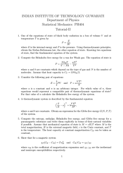
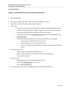

© Copyright 2026