
Variational Methods for Medical Ultrasound Imaging
W ESTFÄLISCHE
W ILHELMS -U NIVERSITÄT
M ÜNSTER
> Variational Methods for
Medical Ultrasound Imaging
Daniel Tenbrinck
- 2013 -
wissen leben
WWU Münster
Variational Methods for
Medical Ultrasound Imaging
Fach: Informatik
Inaugural-Dissertation zur Erlangung des
Doktorgrades der Naturwissenschaften
- Dr. rer. nat. im Fachbereich Mathematik und Informatik
der Mathematisch-Naturwissenschaftlichen Fakultät
der Westfälischen Wilhelms-Universität Münster
vorgelegt von
Daniel Tenbrinck
- 2013 -
Dekan:
Prof. Dr. Martin Stein
Erster Gutachter:
Prof. Dr. Xiaoyi Jiang
(Westf¨alische Wilhelms-Universit¨at M¨
unster)
Zweiter Gutachter:
Prof. Dr. Martin Burger
(Westf¨alische Wilhelms-Universit¨at M¨
unster)
Tag der m¨
undlichen Pr¨
ufung:
Tag der Promotion:
i
Abstract
This thesis is focused on variational methods for fully-automatic processing and analysis
of medical ultrasound images. In particular, the e↵ect of appropriate data modeling in
the presence of non-Gaussian noise is investigated for typical computer vision tasks.
Novel methods for segmentation and motion estimation of medical ultrasound images
are developed and evaluated qualitatively and quantitatively on both synthetic and real
patient data.
The first part of the thesis is dedicated to the problem of low-level segmentation. Two
di↵erent segmentation concepts are introduced. On the one hand, segmentation is formulated as a statistically motivated inverse problem based on Bayesian modeling. Using
recent results from global convex relaxation, a variational region-based segmentation
framework is proposed. This framework generalizes popular approaches from the literature and o↵ers great flexibility for segmentation of medical images. On the other hand,
the concept of level set methods is elaborated to perform segmentation based on the
results of a discriminant analysis of medical ultrasound images. The proposed method
is compared to the popular Chan-Vese segmentation method.
In the second part of the thesis, the concept of shape modeling and shape analysis is
described to perform high-level segmentation of medical ultrasound images. Motivated
by structural artifacts in the data, e.g., shadowing e↵ects, the latter two segmentation
methods are extended by a shape prior based on Legendre moments. Efficient numerical
schemes for encoding and reconstruction of shapes are discussed and the proposed highlevel segmentation methods are compared to their respective low-level variants.
The last part of the thesis deals with the challenge of motion estimation in medical
ultrasound imaging. A broad overview on optical flow methods is given and typical
assumptions and models are discussed. The inapplicability of the popular intensity constancy constraint is shown for the special case of images perturbed by multiplicative
noise both mathematically and experimentally. Based on the idea of modeling image intensities as random variables, a novel data constraint based on local statistics is proposed
and their validity is proven. The incorporation of this constraint into a variational model
for optical flow estimation leads to a novel method which outperforms state-of-the-art
methods from the literature on medical ultrasound images.
This thesis aims to give a balanced view on the di↵erent stages involved in solving
computer vision tasks in medical imaging: Starting from modeling problems, to their
analysis and efficient numerical realization, to their final application and adaption to
real world conditions.
ii
Keywords: Image Processing, Medical Image Analysis, Denoising, Segmentation, Motion Estimation, Variational Methods, Variational Regularization, Optical Flow, Bayesian
Modeling, Expectation-Maximization Algorithm, Noise Modeling, Additive Gaussian
Noise, Rayleigh Noise, Ultrasound Speckle Noise, Generalized Mumford-Shah Formulation, Chan-Vese Algorithm, Medical Ultrasound Imaging, Echocardiography
Dedicated in memory to my beloved mother.
v
Acknowledgments
Sitting in front of a PhD thesis that is finished to 99%, and thinking about all the
persons who directly and indirectly influenced this work, is a task which should best be
done after a couple of weeks vacation and having a settled mind. However, as always in
academic environments, time is short and the next deadline pushes me to hurry on.
For this reason, I decided to acknowledge only the most important people of my life
in the last few years. I will thank all my other supporters in my very individual way,
namely, by organizing a huge party which will be well-remembered in future days.
First of all, I would like to thank my supervisor and mentor Prof. Dr. Xiaoyi Jiang for
giving me quite early the chance to participate in research and develop my skills. As a
team, we underwent five good years with many exceptional experiences within academic,
but also personally. The thing I appreciated most being in his working group, was the
possibility to adjust my research interests freely within the field of computer vision.
Simultaneously, he always managed to keep me on track, when I got lost in the vast
jungle of ideas, algorithms, and papers.
Prof. Dr. Martin Burger is the next person I would like to thank. Although we are settled
in di↵erent institutes in the Department of Mathematics and Computer Science, we
found many common interests to bridge the gap between these two disciplines. Mentoring
my advances in applied mathematics and being my most feared opponent on the football
court, we had a quite contrary relationship in the last couple of years. Hopefully, I proved
him that computer scientists can do more than ’only’ programming software. My grateful
thanks are dedicated to PD Dr. med. J¨org Stypmann, who introduced me to the field
of cardiology and echocardiography with all his expertise. From him I learned how to
sound like a clinical expert in order to convince even the most critical audiences during
conference talks. I have to admit, that the majority of our best collaborative ideas
originated from social events in M¨
unster’s pubs.
I thank the Department of Cardiology and Angiology, University Hospital of M¨
unster,
who acquired the medical ultrasound data, including echocardiographic data of my own
heart. This work was partly funded by the Deutsche Forschungsgemeinschaft, SFB 656
MoBil (project C3).
In the following I would like to give my special thanks to:
• Alex Sawatzky, who had a great influence on the content of this thesis. Our discussions and ideas led to numerous successful implementations and even papers. I
owe him more than just a crate of ’Lala’.
vi
• Jahn M¨
uller, for accompanying me during these stressful times and sharing all
valuable information with me in the process of getting a PhD degree. While I am
writing these lines, he is still sitting next to me, pushing me forward in order to
celebrate this day with a good glass of Aberlour.
• Selcuk Barlak, for always being the good friend I needed, when university got over
my head. His guidance is one of the main reasons I got this far in academics.
• Michael Fieseler and Fabian Gigengack, who stood next to me in good and in bad
times, and shared the most funny office of the department with me.
• the members of the Institute of Computer Science, for helpful discussions and interesting talks. We always had a great time together and the next get-together-BBQ
is in planning.
• the members of the Institute of Applied Mathematics, for affiliating me and treating
me like one of them. In fact, I managed to get on their internal mailing list STRIKE!
• Caterina Zeppieri, who introduced me to the aesthetical field of calculus of variations, and always had an sympathetic ear for my questions and problems.
• Frank W¨
ubbeling, for many, many helpful discussions and joint scribbling on the
board. Additionally, he was my main source for internal gossip in our institutes.
• Olga Friesen, for her helpful hints on statistical mathematics, which I needed
urgently in the course of my work.
• my proof readers Selcuk Barlak, Michael Fieseler, Fabian Gigengack, and Alex
Sawatzky, who wiped out many, many mistakes and typos from this thesis.
• all of my students, who enriched and inspired my work in the Institute of Computer
Science.
• all my friends, who gave me a decent time in M¨
unster and made me happy.
The most important person in the last years is Anna Cathrin G¨ottsch, who supported
me like no other. She has always been there if I needed someone to care for me and
endure me in times of hard pressure at work. For this I love her and will always admire
her.
Finally, I would like to thank my family, who supported me in these years and gave me
the time to finish my PhD thesis. I know it has been a long time and I owe you many
missed parties and relaxing evenings. I promise we will make up for the lost time.
vii
Contents
List of Algorithms
1
1 Introduction
3
1.1
Motivation . . . . . . . . . . . . . . . . . . . . . . . . . . . . . . . . . . .
4
1.2
Contributions . . . . . . . . . . . . . . . . . . . . . . . . . . . . . . . . .
9
1.3
Organization of this work
. . . . . . . . . . . . . . . . . . . . . . . . . .
2 Mathematical foundations
2.1
2.2
2.3
11
13
Topology and measure theory . . . . . . . . . . . . . . . . . . . . . . . .
13
2.1.1
Topology . . . . . . . . . . . . . . . . . . . . . . . . . . . . . . . .
14
2.1.2
Measure theory . . . . . . . . . . . . . . . . . . . . . . . . . . . .
17
Functional analysis . . . . . . . . . . . . . . . . . . . . . . . . . . . . . .
20
2.2.1
Classical function spaces . . . . . . . . . . . . . . . . . . . . . . .
21
2.2.2
Dual spaces and weak topology . . . . . . . . . . . . . . . . . . .
23
2.2.3
Sobolev spaces . . . . . . . . . . . . . . . . . . . . . . . . . . . .
24
Direct method of calculus of variations . . . . . . . . . . . . . . . . . . .
27
2.3.1
Convex analysis . . . . . . . . . . . . . . . . . . . . . . . . . . . .
28
2.3.2
Existence of minimizers
30
. . . . . . . . . . . . . . . . . . . . . . .
3 Medical Ultrasound Imaging
33
3.1
General principle . . . . . . . . . . . . . . . . . . . . . . . . . . . . . . .
34
3.2
Acquisition modalities . . . . . . . . . . . . . . . . . . . . . . . . . . . .
36
3.3
Physical phenomena . . . . . . . . . . . . . . . . . . . . . . . . . . . . .
38
3.3.1
(Non-)Gaussian noise models . . . . . . . . . . . . . . . . . . . .
42
3.3.2
Structural noise . . . . . . . . . . . . . . . . . . . . . . . . . . . .
47
Ultrasound software phantoms . . . . . . . . . . . . . . . . . . . . . . . .
49
3.4
viii
Contents
4 Region-based segmentation
4.1
4.2
4.3
4.4
4.5
53
Introduction . . . . . . . . . . . . . . . . . . . . . . . . . . . . . . . . . .
54
4.1.1
Tasks and applications for segmentation . . . . . . . . . . . . . .
55
4.1.2
How to segment images? . . . . . . . . . . . . . . . . . . . . . . .
56
4.1.3
Segmentation in medical ultrasound imaging . . . . . . . . . . . .
60
Classical variational segmentation models . . . . . . . . . . . . . . . . . .
63
4.2.1
Mumford-Shah model . . . . . . . . . . . . . . . . . . . . . . . . .
63
4.2.2
Chan-Vese model . . . . . . . . . . . . . . . . . . . . . . . . . . .
65
Variational segmentation framework for region-based segmentation . . . .
67
4.3.1
Motivation . . . . . . . . . . . . . . . . . . . . . . . . . . . . . . .
68
4.3.2
Proposed variational region-based segmentation framework . . . .
68
4.3.3
Physical noise modeling . . . . . . . . . . . . . . . . . . . . . . .
74
4.3.4
Optimal piecewise constant approximation . . . . . . . . . . . . .
78
4.3.5
Numerical realization . . . . . . . . . . . . . . . . . . . . . . . . .
82
4.3.6
Implementation details . . . . . . . . . . . . . . . . . . . . . . . .
88
4.3.7
Results . . . . . . . . . . . . . . . . . . . . . . . . . . . . . . . . .
90
4.3.8
Discussion . . . . . . . . . . . . . . . . . . . . . . . . . . . . . . .
99
Level set methods . . . . . . . . . . . . . . . . . . . . . . . . . . . . . . . 105
4.4.1
Implicit functions and surface representations . . . . . . . . . . . 106
4.4.2
Choice of velocity field V . . . . . . . . . . . . . . . . . . . . . . . 111
4.4.3
Numerical realization . . . . . . . . . . . . . . . . . . . . . . . . . 114
Discriminant analysis based level set segmentation . . . . . . . . . . . . . 123
4.5.1
Motivation . . . . . . . . . . . . . . . . . . . . . . . . . . . . . . . 123
4.5.2
Proposed discriminant analysis based segmentation model . . . . 131
4.5.3
Results . . . . . . . . . . . . . . . . . . . . . . . . . . . . . . . . . 136
4.5.4
Discussion . . . . . . . . . . . . . . . . . . . . . . . . . . . . . . . 143
5 High-level segmentation with shape priors
145
5.1
Introduction . . . . . . . . . . . . . . . . . . . . . . . . . . . . . . . . . . 145
5.2
Concept of shapes . . . . . . . . . . . . . . . . . . . . . . . . . . . . . . . 146
5.3
5.2.1
Shape descriptors . . . . . . . . . . . . . . . . . . . . . . . . . . . 148
5.2.2
Moment-based shape representations . . . . . . . . . . . . . . . . 150
5.2.3
Shape priors for high-level segmentation . . . . . . . . . . . . . . 161
5.2.4
A-priori shape information in medical imaging . . . . . . . . . . . 164
High-level segmentation for medical ultrasound imaging . . . . . . . . . . 166
5.3.1
Motivation . . . . . . . . . . . . . . . . . . . . . . . . . . . . . . . 167
5.3.2
High-level information based on Legendre moments . . . . . . . . 168
5.3.3
Numerical realization of shape update
. . . . . . . . . . . . . . . 171
Contents
5.4
5.5
5.6
ix
Incorporation of shape prior into variational segmentation framework
5.4.1 Bayesian modeling . . . . . . . . . . . . . . . . . . . . . . . .
5.4.2 Numerical realization . . . . . . . . . . . . . . . . . . . . . . .
5.4.3 Implementation details . . . . . . . . . . . . . . . . . . . . . .
5.4.4 Results . . . . . . . . . . . . . . . . . . . . . . . . . . . . . . .
Incorporation of shape prior into level set methods . . . . . . . . . .
5.5.1 Numerical realization . . . . . . . . . . . . . . . . . . . . . . .
5.5.2 Implementation details . . . . . . . . . . . . . . . . . . . . . .
5.5.3 Results . . . . . . . . . . . . . . . . . . . . . . . . . . . . . . .
Discussion . . . . . . . . . . . . . . . . . . . . . . . . . . . . . . . . .
6 Motion analysis
6.1 Introduction . . . . . . . . . . . . . . . . . . . . . . . . . . . .
6.1.1 Tasks and applications of motion analysis . . . . . . .
6.1.2 How to determine motion from images? . . . . . . . . .
6.1.3 Motion estimation in medical image analysis . . . . . .
6.2 Optical flow methods . . . . . . . . . . . . . . . . . . . . . . .
6.2.1 Preliminary conditions . . . . . . . . . . . . . . . . . .
6.2.2 Data constraints . . . . . . . . . . . . . . . . . . . . .
6.2.3 Data fidelity . . . . . . . . . . . . . . . . . . . . . . . .
6.2.4 Regularization . . . . . . . . . . . . . . . . . . . . . . .
6.2.5 Determining optical flow . . . . . . . . . . . . . . . . .
6.3 Histogram-based optical flow for ultrasound imaging . . . . . .
6.3.1 Motivation and observations . . . . . . . . . . . . . . .
6.3.2 Histograms as discrete representations of local statistics
6.3.3 Histogram constancy constraint . . . . . . . . . . . . .
6.3.4 Histogram-based optical flow method . . . . . . . . . .
6.3.5 Implementation . . . . . . . . . . . . . . . . . . . . . .
6.3.6 Results . . . . . . . . . . . . . . . . . . . . . . . . . . .
6.3.7 Discussion . . . . . . . . . . . . . . . . . . . . . . . . .
.
.
.
.
.
.
.
.
.
.
.
.
.
.
.
.
.
.
.
.
.
.
.
.
.
.
.
.
.
.
.
.
.
.
.
.
.
.
.
.
.
.
.
.
.
.
.
.
.
.
.
.
.
.
.
.
.
.
.
.
.
.
.
.
.
.
.
.
.
.
.
.
.
.
.
.
.
.
.
.
.
.
.
.
.
.
.
.
.
.
.
.
.
.
.
.
.
.
.
.
.
.
.
.
.
.
.
.
.
.
172
173
174
177
180
185
186
189
190
194
.
.
.
.
.
.
.
.
.
.
.
.
.
.
.
.
.
.
197
197
198
199
201
207
208
208
211
213
216
220
221
224
227
231
237
243
248
7 Conclusion
253
Bibliography
257
1
List of Algorithms
1
2
3
4
5
Proposed region-based variational segmentation framework . . . . .
Solver for weighted ROF problem (ADMM) . . . . . . . . . . . . .
Reinitialization of a signed distance function . . . . . . . . . . . . .
Chan-Vese segmentation method . . . . . . . . . . . . . . . . . . .
Proposed discriminant analysis based level set segmentation method
.
.
.
.
.
.
.
.
.
.
. 85
. 88
. 121
. 127
. 135
6
7
Proposed variational high-level segmentation framework (ADMM) . . . . 177
Proposed high-level segmentation level set method . . . . . . . . . . . . . 189
8
9
Horn-Schunck optical flow method . . . . . . . . . . . . . . . . . . . . . . 219
Proposed histogram-based optical flow method . . . . . . . . . . . . . . . 237
3
1
Introduction
With the help of new technological developments, medical ultrasound imaging evolved
rapidly in the past decades and became a ’condicio sine qua non’ for diagnostics in clinical routine. Due to its low costs, the absence of radiation, and its real-time capacities,
it is employed in a wide range of applications today, e.g., in prenatal diagnosis and
echocardiography.
As medical ultrasound imaging gained importance for clinical healthcare, the interest
in processing and analysis of ultrasound images simultaneously rose within the computer vision and mathematical image processing community. To tackle the challenging
problems in ultrasound images, e.g., a physical noise phenomena called multiplicative
speckle noise, novel methods have been proposed in the recent years which fundamentally di↵er from standard image processing techniques. Since those methods were mainly
introduced in the context of ultrasound image denoising, the question arises whether the
success of the implementation of non-standard noise models translates to other problems
in ultrasound image analysis and if the improvements are significant enough to justify
the additional computational e↵ort. This thesis addresses the question if non-standard
noise models give any benefit for the main tasks of computer vision in medical ultrasound imaging, i.e., image segmentation and motion estimation, and we propose novel
methods in this context.
In the following sections we give an overview of the content of this work. We start in
Section 1.1 with a short motivation for the use of variational methods in medical image
analysis and in particular for medical ultrasound imaging. The main contributions of
this thesis are listed in Section 1.2. Finally, the organization of this work is outlined in
Section 1.3.
4
1 Introduction
1.1 Motivation
Calculus of variations has a long history within the field of mathematical analysis and a
first sophisticated theory was introduced by Leonhard Euler at the beginning of the 18th
century in order to systematically elaborate the ’Brachistochrone curve’ problem initially
formulated by the Bernoulli brothers. In the last three centuries important contributions
have been made by many mathematicians, e.g., Weierstrass, Lebesgue, Carath´eodory,
Legendre, Hamilton, Dirichlet, Riemann, Gauss, Tonelli, and Hilbert just to mention a
few popular ones. Hence, the calculus of variations evolved to a powerful theory with
useful tools for optimization problems of functionals. Eventually, three of the famous
’Hilbert problems’ were dedicated to this field in 1900. In the past decades these methods
underwent a second peak of attention due to the development of a↵ordable computers,
which are able to solve real-life problems with the help of applied mathematics.
One particular application of the calculus of variations is medical image analysis, which in
general deals with the (semi-)automatic processing, analysis, and interpretation of medical image data from various image modalities, e.g., computed tomography or magnetic
resonance tomography. Typical problems include image denoising, image segmentation,
and quantification. Today, research in computer vision and mathematical image processing assists physicians in classification and interpretation of symptoms and enables
them to make time-efficient and reproducible diagnoses in daily clinical routine and thus
maximize the potential number of treatable patients.
While there are many di↵erent approaches in the field of medical image analysis the
impact of variational methods is indisputable. Although these methods require a deep
understanding of the respective mathematical background, the established theory of
calculus of variations gives a solid foundation for a huge variety of problems in medical
image analysis and thus can be seen as universally applicable in this context.
To utilize variational methods in medical image analysis, one has to model the specific
task as an optimization problem of a functional. Typically, the goal is to find a solution
to problems of the form,
inf
u2X
⇢
E(u) =
Z
⌦
g(~x, u(~x), ru(~x)) d~x
.
(1.1)
Depending on the choice of a suitable Banach space X and the integrand g in (1.1), the
solution u 2 X has to fulfill certain requirements if it exists. In order to model physical
e↵ects in the given image data and to incorporate a-priori knowledge about the expected
solution, a special class of variational methods has been introduced. This formulation
is statistically motivated and is based on Bayesian modeling of Gibbs a-priori densities.
1.1 Motivation
5
This leads to variational problems of the form,
inf D(u) + ↵R(u) ,
u2X
↵>0.
(1.2)
Using the terminology of inverse problems, the data fidelity term D measures the deviation of the solution u 2 X to an assumed physical data model and the regularization
term R enforces certain characteristics of an expected solution.
Physical noise modeling for ultrasound imaging
Within this thesis we are especially interested in non-standard data models for computer
vision tasks in medical ultrasound imaging and hence in more appropriate data fidelity
terms in (1.2). For this reason, implicit and explicit physical noise modeling plays an
important role throughout this work.
The standard data model in computer vision for given image data f reads as,
f = u + ⌘,
(1.3)
where u denotes the unknown exact image and ⌘ represents a global perturbation of u
with normally distributed noise. With respect to the form in (1.3), this model is also
known as additive Gaussian noise and is signal-independent. Gaussian noise is the most
common noise model used in the literature, as it is suitable for a wide range of applications, e.g., digital photography or computed tomography. However, observations and
physical experiments indicate that the noise model in (1.3) is not an appropriate choice
for medical ultrasound images. In this context the term ’multiplicative speckle noise’
has gained attention throughout the ultrasound imaging community and first adaptions
of known methods from mathematical image denoising to this model led to significant
improvements in this field.
Inspired by these recent developments, we are interested in the translation of the findings
in image denoising to other important problems in computer vision and mathematical
image processing. By incorporation of appropriate physical noise models we especially
try to improve the performance of algorithms for image segmentation and motion estimation on medical ultrasound images. In this context we investigate Loupas noise of
the form,
(1.4)
f = u + u2 ⌘ ,
where u denotes the unknown exact image and ⌘ is a global perturbation of u with
normally distributed noise. The noise in (1.4) can be desribed as adaptive because the
bias caused by ⌘ is locally amplified or damped by the magnitude of the original image
6
1 Introduction
signal u. The impact of this multiplicative noise is determined by a physical parameter
0
2
, which depends on the imaging system and the respective application.
Furthermore, under certain conditions another multiplicative noise model has proven to
be feasible for medical ultrasound imaging. In case of Rayleigh distributed noise the
considered data model for f is of the form,
f = uµ ,
(1.5)
where u denotes the unknown exact image and µ represents Rayleigh distributed noise.
Both perturbations in (1.4) and (1.5) are categorized as multiplicative noise and they
are signal-dependent due to the relation to u. They di↵er fundamentally from the case
in (1.3) and it is challenging to design robust methods in presence of these non-Gaussian
noise models. Figure 1.1 illustrates the impact of these three noise models on a onedimensional signal.
400
400
350
350
300
300
250
250
200
200
150
150
100
100
50
50
0
0
−50
−50
0
50
100
150
200
250
300
350
400
(a) Exact signal u
0
50
100
150
200
250
300
350
400
(b) Data f perturbed by add. Gaussian noise
400
400
350
350
300
300
250
250
200
200
150
150
100
100
50
50
0
0
−50
−50
0
50
100
150
200
250
300
350
400
(c) Data f perturbed by Loupas noise
0
50
100
150
200
250
300
350
400
(d) Data f perturbed by Rayleigh noise
Fig. 1.1. One-dimensional visualization of the perturbation of a signal by three
di↵erent noise models typically assumed in medical ultrasound imaging.
1.1 Motivation
(a) Erroneous low-level segmentation
7
(b) Training shapes
Fig. 1.2. An unsatisfying segmentation result of an automatic low-level segmentation method due to missing anatomical structures in (a) motivates the incorporation
of high-level information induced by a set of training shapes in (b).
High-level information based on shape priors
Next to the perturbation of medical ultrasound images by physical noise discussed above,
one also has to deal with structural artifacts, e.g., shadowing e↵ects. Since whole image
regions can be a↵ected by this phenomenon, automatic segmentation methods are likely
to produce erroneous segmentation results on the respective data sets. Especially lowlevel segmentation algorithms are notably prone to structural artifacts as they are based
on intrinsic image features only. Figure 1.2a shows an unsatisfying segmentation result
of such a method due to missing anatomical structures near the valvular region of the
left ventricle in a human myocardium.
For this reason, several contributions to the field of ultrasound image segmentation
proposed the incorporation of high-level information by means of a shape prior. The
main intention of using high-level information during the process of segmentation is
to stabilize a method in the presence of physical image noise and structural artifacts.
Figure 1.2b shows a small part of a training data set consisting of left ventricle shapes
delineated by medical experts, which is used for high-level segmentation of medical
ultrasound images.
However, to the best of our knowledge it has not been investigated in the literature so
far, if realistic data modeling, e.g., physical noise modeling, has any significant impact
on the segmentation results of such high-level approaches. Due to this, we evaluate in
the course of this thesis if it is profitable to perform physical noise modeling next to the
incorporation of a-priori knowledge about the shape to be segmented.
8
1 Introduction
Motion estimation in ultrasound imaging
Motion estimation plays a key role for the assessment of medical parameters in computerassisted diagnosis, e.g., in echocardiography. In the context of echocardiographic data it
is often referred to as speckle tracking echocardiography (STE) in clinical environments
and plays an important role in diagnosis and monitoring of cardiovascular diseases and
the identification of abnormal cardiac motion. Next to measurements of the atrial chambers’ motion, many diagnosis protocols are specialized for STE of the left ventricle, e.g.,
for revealing myocardial infarctions and scarred tissue.
Typically, STE is done by manual contour delineation performed by a physician, followed by automatic contour tracing over time. This semiautomatic o✏ine-procedure is
time consuming as it requires the physician to segment the endocardium manually. Furthermore, it is clear that speckle tracking is difficult in the presence of speckle noise and
in low contrast regions due to the loss of signal intensity. This makes speckle tracking a
very challenging task and motivates the goal of developing robust and fully automatic
motion estimation methods for medical ultrasound imaging.
Most proposed methods for motion estimation on medical ultrasound data are derived
from classical computer vision concepts and include registration and optical flow methods. One typical assumption in the context of optical flow methods is the intensity
constancy constraint (ICC), which is given in the case of two-dimensional data by,
I(x, y, t) = I(x + u, y + v, t + 1) .
(1.6)
Obviously, this constraint is seldom fulfilled on real data, but using quadratic distance
measures in combination with additional smoothness constraints has proven to lead to
satisfying results of optical flow methods on most type of images in computer vision.
However, the situation is di↵erent for medical ultrasound images, due to the presence of
physical phenomena such as multiplicative speckle noise. In particular, we are able to
show mathematically that the ICC in (1.6) and its higher order variants are not valid
in the presence of Loupas noise and results of methods based on these constraints are
prone to get biased.
To overcome this problem, it is feasible to model the signal intensities of image pixels
as discrete random variables and use the local distribution of these random variables as
feature for motion estimation. It turns out that this feature leads to more robust and
accurate optical flow estimation results and the correctness of a newly derived constraint
based on local statistics can be shown both mathematically as well as experimentally.
1.2 Contributions
9
1.2 Contributions
In this thesis we address typical tasks of computer vision and mathematical image processing for medical ultrasound imaging and utilize variational methods to model these
tasks appropriately. The main contribution in this work is the incorporation of a-priori
knowledge about the image formation process in ultrasound images and the development
of novel variational formulations which are based on non-standard data fidelity terms.
We elaborate di↵erent ways to increase the robustness of computer vision concepts in
the presence of perturbations in ultrasound imaging and investigate the impact of both
implicit and explicit physical noise modeling on the results of the proposed methods.
In general, we aim to present a balanced view on the process of observation-based modeling, analysis of the proposed variational formulations, and their respective numerical
realization. Furthermore, this thesis gives a broad overview on related techniques and
introduces the related topics in a top-down manner. All proposed models are evaluated
on synthetic data and/or real patient data from daily clinical routine.
Low-level segmentation
We investigate two di↵erent concepts of low-level segmentation. We propose a regionbased variational segmentation framework which explicitly incorporates physical noise
models using the theory of Bayesian modeling. We perform segmentation using singular
energies and also methods recently proposed from the field of global convex relaxation.
The generality and modularity of this segmentation framework gives a huge amount of
flexibility to perform segmentation tasks in medical imaging and allows to model the
image intensities for each region separately. In particular, we realized:
• four di↵erent data fidelity terms corresponding to additive Gaussian noise, Loupas
noise, Rayleigh noise, and Poisson noise,
• four di↵erent regularization terms, i.e., piecewise-constant approximation, H 1 seminorm, Fisher information, and total variation.
For a two-phase segmentation task, e.g., partitioning the image domain in background
region and object-of-interest, this leads to (4 ⇥ 4)2 = 256 possible segmentation setups. Naturally, it is not possible to evaluate all options of this proposed segmentation
framework in the course of this thesis, due to the vast time e↵ort needed for parameter optimization. Hence, we concentrate on three noise models typically assumed for
medical ultrasound imaging and piecewise-constant approximations as used, e.g., in the
popular Chan-Vese segmentation method.
10
1 Introduction
In the context of low-level segmentation we analyze the just mentioned Chan-Vese
method and observe that its level set based realization leads to erroneous segmentation
results on medical ultrasound images. We elaborate di↵erent reasons for this observation
such as the existence of local minima and an inappropriate data fidelity term. To overcome these drawbacks, we propose a novel segmentation formulation that partitions the
image domain by incorporating valuable information from the image histogram using
discriminant analysis. The superiority of the proposed method is demonstrated on real
patient data from echocardiographic examinations.
High-level segmentation
As indicated in Section 1.1, structural artifacts often lead to the necessity of incorporating high-level information into the process of segmentation. Within this thesis we
discuss di↵erent concepts of shape description and focus on moment-based representations of image regions. We discuss the advantages and disadvantages of geometric,
Legendre, and Zernike moments from an application view and give details on efficient
implementations of these. In particular we give a formal proof for the correctness of
an iterative construction formula for Legendre coefficients, which eases the challenge of
evaluating high-order Legendre polynomials. Based on Legendre moments we construct
a shape prior as realization of a Rosenblatt-Parzen estimator, known from statistics.
Although several works propose the use of shape priors to increase the robustness of
segmentation methods, it is unclear if the influence of these shape priors make physical noise modeling unnecessary for medical ultrasound data. Hence, we extend the two
proposed low-level segmentation concepts by the shape prior mentioned above and investigate the impact of physical noise modeling on robustness and accuracy of high-level
segmentation within this thesis. In this context we perform qualitative and quantitative
studies on real patient data from echocardiography.
Motion estimation
Finally, we address the problem of fully automatic motion estimation on medical ultrasound images and give a broad introduction to this topic. We focus on optical flow
methods and summarize the most common assumptions, constraints, data fidelity terms,
and regularization methods from this field. We are able to show mathematically and
experimentally that the most popular constraints, i.e., the ICC in (1.6) and its variants,
lead to erroneously corresponding pixels in presence of multiplicative noise and hence to
biased results of motion estimation.
1.3 Organization of this work
11
By observing the characteristics of speckle noise in medical ultrasound images, we propose a novel feature based on local statistics and deduce an alternative constraint to
overcome the limitations of the ICC. The so-called histogram constancy contraint is embedded in a variational formulation and compared to the closely related Horn-Schunck
optical flow method. We show the validity of the histogram-based optical flow method
mathematically and give a formal proof for the existence of unique minimizers by using
the direct method of calculus of variations. The new model is evaluated on both synthetic as well as real patient data and we show that it outperforms recent state-of-the-art
methods from the literature on medical ultrasound data.
1.3 Organization of this work
In Chapter 2 we provide the mathematical foundation for the modeling and analysis of
computer vision tasks in medical ultrasound imaging. In particular, we give the basic
tools needed to show the existence of minimizers of variational formulations based on
concepts from functional analysis, e.g., Sobolev spaces.
A short introduction to the application of medical ultrasound imaging in Chapter 3 motivates the development of non-standard methods for this imaging modality and outlines
the challenges induced by physical phenomena such as speckle noise and shadowing effects.
Chapter 4 is subdivided into two semantic parts both focused on low-level segmentation. In the first half we discuss classical segmentation formulations from the literature
and propose the region-based variational segmentation framework which allows to incorporate di↵erent noise models and regularization terms. In the second part we give a
introduction to the concept of level set segmentation and provide the foundation for the
numerical realization of a novel segmentation formulation based on discriminant analysis.
We give an introduction to the concept of shape representation and its use for medical
ultrasound segmentation in Chapter 5. Both proposed low-level segmentation methods
from the last chapter are extended by a shape prior based on Legendre moments. We
investigate the impact of physical noise modeling on high-level segmentation and evaluate the use of di↵erent data fidelity terms in this context.
Finally, we discuss the challenge of fully automatic motion estimation for medical ultrasound images in Chapter 6. We give a broad overview on optical flow methods and prove
the inapplicability of the fundamental assumption of intensity constancy for ultrasound
images. A new constraint based on local statistics is introduced and its superiority is
shown mathematically and experimentally.
13
2
Mathematical foundations
In this chapter we aim to give a solid foundation for the mathematical arguments needed
to formulate variational problems in medical ultrasound imaging. We start from the very
basics of topology and measure theory in Section 2.1 to be able to introduce more abstract
concepts in the course of this chapter, e.g., Lebesgue spaces. As already indicated in
Section 1, we are interested in finding optimal solutions for minimization problems based
on functionals. Since a solution of such a problem is a function which is determined to
fulfill certain requirements depending on the application at focus, it is reasonable to give
the most important relations from the field of functional analysis in Section 2.2. Based
on the concepts of Sobolev spaces and weak converging sequences, we are able to provide
tools from the direct method of calculus of variations, which are needed for the analysis
of variational problems and the proof for existence of minimizers.
Since the mathematical relations in this chapter are well-known and not in the focus of
this thesis, we only give the needed information and refrain to describe these concepts in
more detail. Hence, the following descriptions have to be understood as reference text
for later chapters.
2.1 Topology and measure theory
We start with an introduction to general topological spaces in Section 2.1.1 and refine
basic concepts such as open sets, continuity, and converging sequences for metric spaces
and finally define vector spaces.
In Section 2.1.2 we start with the definition of measurable spaces and -algebras and give
important examples, e.g., the Lebesgue -algebra. Introducing measurable functions we
are able to reproduce the construction of the Lebesgue integral.
14
2 Mathematical foundations
2.1.1 Topology
The following definitions in the context of topological and metric spaces are based on
[69, §1-3] written by Forster and [5, §0] by Alt.
Definition 2.1.1 (Topological spaces and open sets). Let X be a basic set, I an arbitrary
index set and J a finite index set. A set T containing subsets of X is called topology,
if the following properties are fulfilled,
• the empty set {} and X itself are elements in T ,
S
• any union i2I Xi of elements Xi 2 T is an element in T ,
T
• any finite section j2J Xj of elements Xj 2 T is an element in T .
The subsets of X which are in the topology T are called open sets and the basic set X
with the topology T is called a topological space (X, T ). Elements of the basic set X in
a topological space (X, T ) are called points.
Example 2.1.2 (Real vector spaces Rn with canonical topology). The set of all open
intervals (a, b) ⇢ R induces a topology for the set of real numbers R. Accordingly, for
real vector spaces Rn one possible topology is the product topology of the latter one, which
is given by the set of Cartesian products of open intervals (a1 , b1 ) ⇥ · · · ⇥ (an , bn ) ⇢ Rn .
Definition 2.1.3 (Continuity in topological spaces). Let (X1 , T1 ) and (X2 , T2 ) be topological spaces. A function f : (X1 , T1 ) ! (X2 , T2 ) is called continuous, if the preimage
of any open set Y 2 T2 is open, i.e., f 1 (Y ) 2 T1 .
Definition 2.1.4 (Neighborhood of points). Let (X, T ) be a topological space and x 2 X
a point. A subset V ⇢ X with x 2 V is called neighborhood of x if there exists a open
set U 2 T which contains x with U ⇢ V .
Definition 2.1.5 (Sequences in topological spaces). Let (X, T ) be a topological space.
A function : N ! X is called sequence in X. We define elements of the sequence
as xn := (n) and denote with (xn ) := (xn )n2N the whole sequence. A subsequence
(xnk )k2N of (xn ) is a sequence induced by a strictly monotonic function : N ! N with
xnk := x (k) = ( (k)).
Definition 2.1.6 (Convergent sequences in topological spaces). Let (X, T ) be a topological space. A sequence (xn ) in X is called convergent to a point x 2 X, if for every
open neighborhood Y 2 T of x there exists a n0 2 N such that xn 2 Y for all n n0 .
2.1 Topology and measure theory
15
Definition 2.1.7 (Compactness in topological spaces). Let (X, T ) be a topological space.
S
A subset K ⇢ X is called compact if every open cover K ⇢ i2I Ui (with Ui 2 T ) has
S
a finite subcover such that K ⇢ j2J Uj for Uj 2 T , for which I is an arbitrary index
set and J ⇢ I is a finite index set. A topological space (X, T ) is called locally compact
if every point x 2 X has a compact neighborhood.
Definition 2.1.8 (Separability and Hausdor↵ spaces). Let (X, T ) be a topological space.
Two points x, y 2 X are called separable in X if there exist a neighborhood U ⇢ X of x
and a neighborhood V ⇢ X of y, such that the section of these neighborhoods is empty,
i.e., U \ V = ;. If any distinct points x, y 2 X are separable then we call (X, T ) a
Hausdor↵ space.
Metric spaces
In order to measure distances in topological spaces in a meaningful way it is mandatory
to define a metric space and refine the concepts introduced above.
Definition 2.1.9 (Metric spaces). Let X be a basic set. A function d : X ⇥ X ! R is
called a metric if the following properties are fulfilled for arbitrary elements x, y, z 2 X,
• d(x, y)
0
^
d(x, y) = 0 , x = y ,
• d(x, y) = d(y, x) ,
• d(x, z) d(x, y) + d(y, z) .
A basic set X with a metric d on X is called a metric space (X, d). The elements x 2 X
are called points.
Definition 2.1.10 (Open ball in metric spaces). For a point x 2 (X, d) in a metric
space (X, d) the open ball Br (x) ⇢ X with radius r > 0 is defined as the set
Br (x) := {y 2 X | d(x, y) < r} .
Remark 2.1.11. A metric space (X, d) is a topological space in the sense of Definition
2.1.1. This is due to the fact, that the metric d induces a topology on the basic set X.
In this case a set U ⇢ X is open in the induced topology T if each point x 2 U has an
open ball which is fully contained in U , i.e.,
8 x 2 U 9 r > 0 : Br (x) ⇢ U .
16
2 Mathematical foundations
Remark 2.1.12 (Converging sequences in metric spaces). Let (X, d) be a metric space.
A sequence (xn ) is called convergent to a point x 2 X, if for every r > 0 there exists a
n0 2 N, such that xn 2 Br (x) for all n n0 . Equivalently, a sequence is convergent if
for every ✏ > 0 there exists a n0 2 N, such that d(xn , x) < ✏ for all n n0 .
Definition 2.1.13 (Cauchy sequences in metric spaces). Let (X, d) be a metric space.
A sequence (xn ) in X is called Cauchy sequence, if for every ✏ > 0 there exists a n0 2 N,
such that d(xn , xm ) < ✏ for all n, m n0 .
Definition 2.1.14 (Complete spaces). A metric space (X, d) is called complete, if every
Cauchy sequence (xn ) in X converges to a point x 2 X.
In the case of metric spaces we can give equivalent definitions of continuity and compactness, which are more intuitive compared to the respective Definitions 2.1.3 and 2.1.7.
Definition 2.1.15 ((Sequential) continuity in metric spaces). Let (X, dX ) and (Y, dY )
be metric spaces. A function f : (X, dX ) ! (Y, dY ) is called (sequentially) continuous,
if for every sequence (xn ) in X converging to a point x 2 X the corresponding image
sequence (f (xn )) converges to the point f (x) =: y 2 Y .
Definition 2.1.16 ((Sequential) compactness in metric spaces). Let (X, d) be a metric
space. A subset K ⇢ X is called (sequentially) compact, if every sequence (xn ) ⇢ K
has a subsequence (xnk ) which converges to a point x 2 K.
Definition 2.1.17 (Normed vector spaces). Let V be a vector space over a field K, e.g.,
K = R. A norm on V is a function || · || : V
! R 0 , which fulfills the following
properties for vectors x, y 2 V and scalars a 2 K,
• ||x|| = 0 ) x = 0 ,
• ||ax|| = |a| · ||x|| ,
• ||x + y|| ||x|| + ||y|| .
Here, | · | is the absolute value in K. The pair (V, || · ||) is called a normed vector space.
Remark 2.1.18. A normed vector space (V, || · ||) is a metric space in the sense of
Definition 2.1.9. Using the homogeneity property of the norm ||·|| for a = 1 and a = 0,
respectively, one can deduce symmetry of the norm and the identity of indiscernibles, i.e.,
• ||x
y|| = ||y
x|| ,
• ||x|| = 0 , x = 0 .
2.1 Topology and measure theory
17
Hence, (V, || · ||) can be interpreted as metric space (V, d) by setting the metric d as
d(x, y) := ||x y||. In particular, (V, || · ||) is a topological space by Remark 2.1.11 with
the topology induced by the norm || · ||.
Definition 2.1.19 (Banach spaces). A normed vector space (V, || · ||) is called Banach
space, if it is complete.
Definition 2.1.20 (Euclidean vector spaces). An n-dimensional Euclidean vector space
En is a real normed vector space together with an Euclidean structure. This structure
is induced by the definition of a scalar product on vectors v, w 2 En , i.e.,
v
u n
uX
hv, wi = v · w := t
vi w i .
i=1
The Euclidean scalar products allows to measure angles between vectors and induces a
norm on En by ||v|| := hv, vi.
Example 2.1.21. The vector space Rn together with the standard inner product on Rn
is an Euclidean vector space.
2.1.2 Measure theory
The following definitions introduce the basic concepts of measure theory needed for the
proper construction of the Lebesgue integral, which we need in the context of Lebesgue
spaces in later Sections. We follow [53, §2] by De Barra.
Definition 2.1.22 ( -Algebra and measurable spaces). Let ⌦ be a basic set, P(⌦) the
power set of ⌦, and I an arbitrary index set. A set A ⇢ P(⌦) containing subsets of ⌦
is called -algebra, if the following properties are fulfilled,
• ⌦ itself is an element in A,
• for A 2 A its complement Ac is also an element in A,
S
• any union i2I Ai of elements Ai 2 A is element in A.
The pair (⌦, A) is called measurable space and a subset Ai 2 A is called measurable
set.
Definition 2.1.23 (Measure and measure space). Let ⌦ be a set, I an arbitrary index
set, and A a -algebra over ⌦. A function µ : A ! R [ {+1} is called measure if
the following properties are fulfilled,
18
2 Mathematical foundations
• µ(;) = 0 ,
• µ(A)
• µ
S
0 for A 2 A ,
i2I Ai
=
P
i2I
µ(Ai ) ,
with Ai \ Aj = ; for i 6= j .
The triple (⌦, A, µ) is called a measure space.
Definition 2.1.24 (Borel -algebra). Let (⌦, T ) be a topological space. The Borel algebra B(⌦) is uniquely defined as the smallest -algebra that contains all open sets of
⌦ with respect to the corresponding topology T .
Definition 2.1.25 (Borel measure). Let (X, T ) be a locally compact Hausdor↵ space and
B(X) the Borel -algebra on X. Any measure µ on B(X) is called Borel measure on
X, if for each point x 2 X there exists an open neighborhood U , such that µ(U ) < +1.
Remark 2.1.26 (Lebesgue-Borel measure). The canonical Borel measure µ on the measurable space (Rn , B(Rn )) is called Lebesgue-Borel measure. It is chosen such that it
assigns each interval [a, b] ⇢ R (for n = 1) its length µ([a, b]) = b a. Analogously,
it assigns each rectangle its area and each cuboid its volume (for n = 2 and n = 3,
respectively). Hence it is uniquely defined by the property,
µ([a1 , b1 ] ⇥ · · · ⇥ [an , bn ]) = (b1
a1 ) · · · (bn
an ) .
The Lebesgue-Borel measure µ is translation-invariant and normed, i.e., µ([0, 1]) = 1.
However, µ is not complete, i.e., not every subset of a null set is measurable.
Definition 2.1.27 (Lebesgue -algebra and Lebesgue measure). Let (Rn , B(Rn ), µ) be
a measure space with the Lebesgue-Borel measure of the n-dimensional Euclidean vector
space Rn . The Lebesgue -algebra L(Rn ) is defined by adding all sets A ⇢ Rn to
B(Rn ) which are between two Borel sets B1 , B2 2 B(Rn ) with equal Borel measure, i.e.,
B1 ⇢ A ⇢ B2 with µ(B1 ) = µ(B2 ). By this extension the Lebesgue-Borel measure µ gets
completed and hence is called the Lebesgue measure . Naturally, the measure (A) is
determined by B1 and B2 , since (B2 \B1 ) = 0 and thus (A) = (B1 ) = (B2 ).
Definition 2.1.28 (Lebesgue measure null set). Let (Rn , L(Rn ), ) be the measure space
with the Lebesgue measure of the n-dimensional Euclidean vector space Rn . A Lebesgue
measurable set N 2 L(Rn ) is called Lebesgue measure null set, if the Lebesgue measure
of N is zero, i.e., (N ) = 0. Any non-measurable subset of a Lebesgue measure null
set is considered to be neglible from a measure-theoretical point-of-view and hence its
Lebesgue measure is defined as zero as well.
2.1 Topology and measure theory
19
Definition 2.1.29 (Measurable functions). Let (⌦1 , A1 ) and (⌦2 , A2 ) be measurable
spaces. A function
f : (⌦1 , A1 ) ! (⌦2 , A2 )
is called measurable if any measurable set A 2 A2 has a measurable preimage in A1 ,
i.e., f 1 (A) 2 A1 .
Following [53, §3], we are now able to introduce the Lebesgue integral for measurable
functions.
Definition 2.1.30 (Construction of the Lebesgue integral). Let (Rn , L(Rn ), ) be the
Euclidean measure space of Rn with the Lebesgue measure and f : ⌦ ⇢ Rn ! R be a
Lebesgue measurable function. The Lebesgue integral of f is constructed in three steps.
i) First, one considers simple functions gn : ⌦ ! R 0 which are non-negative,
Lebesgue measurable, and only have n 2 N di↵erent values. These elementary
functions can be written as
n
X
gn =
↵ i Ai ,
i=1
n
for which the Ai 2 L(Rn ) are Lebesgue measurable sets and fulfill ⌦ = [˙ i=1 Ai ,
Ai denotes the characteristic function of Ai , and the ↵i 2 R 0 represent the nonnegative real values of gn . Then the Lebesgue integral of simple functions gn can be
computed using the Lebesgue measure , i.e.,
Z
gn d
=
⌦
Z X
n
↵i
Ai
⌦ i=1
d
:=
n
X
↵i (Ai ) .
i=1
ii) Next, one considers general non-negative functions f : ⌦ ! R 0 which are
Lebesgue measurable. These functions can be written as (pointwise) limit of simple
functions from step i). Thus, for a sequence of simple functions (gn )n2N which converge pointwise and monotonically increasing against f , the Lebesgue integral of f
is defined as the limit of these approximating simple functions, i.e.,
Z
fd
⌦
:=
Z
lim gn d
⌦ n!1
= lim
n!1
Z
gn d .
⌦
The last equality holds due to the monotone convergence theorem [53, §3, Theorem
4]. Since the Lebesgue measure is complete, this limit process is well-defined.
20
2 Mathematical foundations
iii) Last, one considers arbitrary functions f : ⌦ ! R that are Lebesgue measurable.
By defining
f + := max{f, 0} ,
f := max{ f, 0}
it is possible to split f into its positive and negative parts by f = f + f . Thus,
using the construction in step ii) the Lebesgue integral of f is defined as
Z
fd
:=
⌦
Z
Z
+
f d
⌦
f d .
⌦
The function f is called Lebesgue integrable if both integrals above are finite, i.e.,
Z
+
f d
^
< +1
⌦
Equivalently, one may require that
R
⌦
Z
f d
< +1 .
⌦
|f | d is finite.
2.2 Functional analysis
Based on the very basic concepts introduced in Section 2.1, one is able to formulate
more abstract relationships in the context of infinite-dimensional function spaces and in
particular Lebesgue spaces. To give the needed definitions from the field of functional
analysis we follow the books of Alt [5, §1-3] and Dacarogna [45, §1].
Definition 2.2.1 (Linear operator). Let X, Y be two real vector spaces. A function
F : X ! Y is called a linear operator on X, if the following properties are fulfilled,
i) F (x + y) = F (x) + F (y) ,
ii) F ( x) =
F (x) ,
for all x, y 2 X ,
for all x 2 X,
2R.
Definition 2.2.2 (Continuous operator). Let X, Y be real normed vector spaces and
F : X ! Y a linear operator. We call F continuous if it is bounded, i.e., there exists a
constant C 0 such that,
||F (x)||Y C||x||X
for all x 2 X .
Example 2.2.3. As a canonical example for continuous linear operators between two
finite-dimensional normed spaces X, Y , one might think about the multiplication of vectors x 2 X with a fixed matrix A.
2.2 Functional analysis
21
Definition 2.2.4 (Space of continuous linear operators T ). Let X, Y be real normed
vector spaces. The vector space of continuous linear operators T (X, Y ) is defined as,
T (X, Y ) := {F : X ! Y | F is continuous and linear } .
For a given F 2 T (X, Y ) the operatornorm || · ||T (X,Y ) is given by,
||F ||T (X,Y ) :=
sup ||F x||Y .
||x||X 1
If Y is even a Banach space, then T (X, Y ) is also a Banach space [5, Theorem 3.3].
2.2.1 Classical function spaces
In the following we introduce classical function spaces as they are investigated in functional analysis, e.g., Lebesgue spaces. These infinite dimensional function spaces allow
us to introduce Sobolev spaces in later sections. The definitions given here basically
follow [5, §1.7 and §1.10] and [45, §1.2]
Definition 2.2.5 (Function spaces C m ). Let ⌦ ⇢ Rn be an open, bounded subset and
let m 0. Further let ↵ 2 Nn0 be a n-dimensional multi-index. Then the vector space of
the m-times continuously di↵erentiable functions C m (⌦) is defined as,
C m (⌦) = {f : ⌦ ! R | f is m-times continuously di↵erentiable in ⌦ and
D↵ is continuously extendable on ⌦ for |↵| m} .
Here, |↵| denotes the sum of the n components of ↵ and the di↵erential operator D↵ is
defined as,
@ |↵|
D ↵ = ↵1
.
(2.1)
@ x 1 . . . @ ↵n x n
The function space C m (⌦) provided with the norm given by,
||f ||C m (⌦) =
X
0|↵|m
||D↵ f ||1 ,
is a Banach space.
The vector space C 1 (⌦) is thus the space of infinitely di↵erentiable functions.
22
2 Mathematical foundations
Definition 2.2.6 (Function spaces L p ). Let (⌦, L(⌦), ) be a measure space with the
Lebesgue measure and 1 p < 1. The set of functions f : ⌦ ! R which are measurable
and Lebesgue integrable in the p-th power induce a vector space,
L (⌦) := { f : ⌦ ! R | f is Lebesgue measurable,
p
Z
⌦
|f (x)|p d (x) < 1 } .
The function space L p can be provided with a seminorm given by,
||f ||L p (⌦) :=
✓Z
p
⌦
|f (x)| d (x)
◆ p1
.
(2.2)
In the case p = 1 the seminorm in (2.2) is replaced by a seminorm based on the essential
supremum, i.e.,
||f ||L 1 (⌦) := ess sup |f (x)| .
x2⌦
Remark 2.2.7. Due to the existence of Lebesgue measure null sets the function || · ||L p
in (2.2) is only a seminorm. Indeed, let N 2 L(⌦) be a Lebesgue measure null set, i.e.,
(N ) = 0. Then for the characteristic function N of N we get || N ||L p = 0 although
p
N 6⌘ 0. Thus, it is reasonable to consider a proper factor space of L .
Definition 2.2.8 (Lebesgue spaces Lp ). Let (⌦, L(⌦), ) be a measure space with the
Lebesgue measure and 1 p 1. Further, let N p (⌦) be the set of functions f 2 L p (⌦)
with ||f ||L p = 0. Then the factor space
Lp (⌦) := L p (⌦) / N p
is a normed vector space with the norm induced by (2.2). The space Lp is complete and
hence a Banach space which is called Lebesgue space.
We further define the space of locally Lebesgue integrable functions Lploc (⌦) as,
Lploc (⌦) := {f : ⌦ ! R | f 2 Lp (C) for all C ⇢ ⌦ compact } .
Remark 2.2.9. By definition the vectors in Lp are not functions f anymore, but equivalence classes [f ]. In particular, two functions f1 and f2 are in the same equivalence
class if they are equal -almost everywhere on ⌦, i.e., up to Lebesgue measure null sets.
Thus, the seminorm || · ||L p in (2.2) gets a norm in Lp (⌦) by || [f ] ||Lp := ||f ||L p .
2.2 Functional analysis
23
Definition 2.2.10 (Strong convergence in Lp ). Let ⌦ ⇢ Rn be an open subset. Further
let 1 p 1 and (un )n2N ⇢ Lp (⌦). The sequence (un ) (strongly) converges to a
function u 2 Lp (⌦), if
lim ||un u||Lp (⌦) = 0 .
n!1
In this context we introduce the notation (un ) ! u in Lp (⌦) for the strong convergence.
2.2.2 Dual spaces and weak topology
Since we are interested in compactness results in infinite-dimensional function spaces, it
is reasonable to introduce the concept of dual spaces and weak convergence. We follow
the definitions in [5, §3-5] and [45, §1.3].
Definition 2.2.11 (Continuous dual spaces). Let X be a normed vector space. Then
the (continuous) dual space X 0 of X is defined as the vector space of linear functionals
on X (cf. Definition 2.2.4), i.e.,
X 0 := T (X, R) = { F : X ! R | F is continuous and linear } .
The weak topology of X with respect to X 0 is the coarsest topology on X for which the
linear functionals in X 0 are continuous in the sense of Definition 2.2.2.
For a Banach space X the dual space X 00 := (X 0 )0 of X 0 is called bidual space of X.
Definition 2.2.12 (Reflexive spaces). If the canonical embedding of a Banach space X
into its bidual space X ,! X 00 is an isomorphism, it is called a reflexive space.
Definition 2.2.13 (H¨older conjugates). Let 1 < p, q < 1, then p and q are called
H¨older conjugates to each other, if the following equality holds,
1
1
+
= 1.
p
q
(2.3)
If p = 1, then q = 1 is called its H¨older conjugate and vice versa.
Example 2.2.14 (Dual spaces of Lp ). The following properties exist for dual spaces of
Lp (⌦).
i) Let 1 p 1 and let q be the H¨older conjugate of p. Then the space Lq (⌦) is the
dual space of Lp (⌦) in the sense of Definition 2.2.11.
ii) For 1 < p < 1 the space Lp (⌦) is reflexive. Note that L1 (⌦) and L1 (⌦) are
non-reflexive.
24
2 Mathematical foundations
Definition 2.2.15 (Weak convergence in Lp ). Let ⌦ ⇢ Rm be an open subset.
• Let 1 p < 1 and (un )n2N ⇢ Lp (⌦). The sequence (un ) weakly converges to a
function u 2 Lp (⌦), if
lim
n!1
Z
(un
u)' dx = 0
⌦
for all ' 2 Lq (⌦) .
In this context we introduce the notation (un ) * u in Lp (⌦) for the weak convergence.
• In the case p = 1 a sequence (un )n2N ⇢ L1 (⌦) weakly-⇤ converges to a function
u 2 L1 (⌦), if
lim
n!1
Z
(un
⌦
u)' dx = 0
for all ' 2 L1 (⌦) .
⇤
In this context we introduce the notation (un ) * u in L1 (⌦) for the weak-⇤ convergence.
The following theorem can be interpreted as a generalization of the Bolzano-Weierstrass
theorem, which cannot be applied directly for infinite-dimensional spaces. However,
using the concept of the weak topology on a reflexive Banach space, we are able to
utilize similar compactness results.
Theorem 2.2.16. Let X be a reflexive Banach space. Then any bounded sequence
(xn )n2N ⇢ X is compact with respect to the weak convergence, i.e., if there exists a
constant C > 0 such that ||xi ||X C for all i 2 N, then there exists a subsequence
(xnk )k2N ⇢ (xn ), such that
xnk * xˆ 2 X .
Proof. [5, Theorem 5.7]
2.2.3 Sobolev spaces
Finally, we are able to introduce the concept of weak di↵erentiability and consequently
the well-known Sobolev spaces, which play a key role in the formulation of variational
models in mathematical image processing due to their properties. We follow the definitions in [5, §1.15] and [45, §1.4].
2.2 Functional analysis
25
Definition 2.2.17 (Weak di↵erentiability). Let ⌦ ⇢ Rn and f 2 Lploc (⌦) (cf. Definition
2.2.8). Further, let ↵ 2 Nn0 be a n-dimensional multi-index. The function f is called
weakly di↵erentiable, if there exists a function g 2 Lploc (⌦), such that for all test functions
' 2 Cc1 (⌦),
Z
Z
f (x)D↵ '(x) dx = ( 1)|↵|
⌦
g(x)'(x) dx .
⌦
Here, |↵| denotes the sum of the n components of ↵ and the di↵erential operator D↵ is
defined as in (2.1). The function D↵ f := g is called ↵-th weak derivative of f .
Remark 2.2.18. In the context of weak derivatives the following properties can be shown
according to [45, §1.27],
i) If the ↵-th weak derivative of a function exists, it is unique a.e. on ⌦.
ii) All important rules of di↵erentiation can be generalized in a way that they are compatible with the definition of weak di↵erentiability.
iii) If a function f 2 Lp (⌦) is di↵erentiable in the conventional sense it is in particular
weakly di↵erentiable and its weak derivative is identical with its (strong) derivative.
Definition 2.2.19 (Sobolev spaces W k,p ). Let ⌦ ⇢ Rn be an open subset. Further, let
↵ 2 Nn0 be a n-dimensional multi-index, k 1 an integer, and 1 p 1. The set of
functions whose weak derivatives are Lebesgue integrable is given by,
W k,p (⌦) := { f : ⌦ ! R | D↵ f 2 Lp (⌦) for all 0 |↵| k } .
The Banach space W k,p (⌦) with the norm
||f ||W k,p (⌦) :=
is called Sobolev space.
8
>
>
>
<
>
>
>
:
P
0|↵|k
||D↵ f ||pLp (⌦)
max ||D↵ f ||L1 (⌦)
0|↵|k
! p1
if 1 p < 1
if p = 1
Remark 2.2.20. The following statements further characterize Sobolov spaces,
i) The space W k,p (⌦) is reflexive for 1 < p < 1.
ii) The special case of p = 2 is the only Sobolev space that is also a Hilbert space
and is denoted as H k (⌦) := W k,2 (⌦). This is a direct consequence of the Riesz
representation theorem, e.g., see [5, Theorem 4.6], and the H¨older inequality as
given in [45, Theorem 1.13].
26
2 Mathematical foundations
Definition 2.2.21 (Convergence in W k,p ). Let ⌦ ⇢ Rn be an open subset. Further let
1 p 1, and (un )n2N ⇢ W k,p (⌦). The sequence (un ) (strongly) converges to a
function u 2 W k,p (⌦), if
lim ||un
n!1
lim ||D↵ un
n!1
u||Lp (⌦) = 0 ,
D↵ u||Lp (⌦) = 0
for all 1 |↵| k .
In this context we introduce the notation (un ) ! u in W k,p (⌦) for the strong convergence in accordance with Definition 2.2.10. Weak convergence in W k,p (⌦) is defined
analogously with respect to Definition 2.2.15.
Remark 2.2.22 (Uniqueness of the limit). The limit of any weakly or strongly converging
sequence (un )n2N ⇢ W k,p (⌦) is unique [45, Remark 1.16].
Remark 2.2.23. Let ⌦ ⇢ Rn be a open bounded set with a Lipschitz boundary and let
1 < p < 1. If for a sequence (un )n2N ⇢ W k,p (⌦) there exists a constant C > 0, such
that ||ui ||W k,p (⌦) C for all i 2 N, then there exists a subsequence (unk )k2N ⇢ (un ) and
uˆ 2 W k,p (⌦) with,
unk * uˆ .
Using the Definition 2.2.19, this is a direct corollary of Theorem 2.2.16.
Generalization of Lp and W k,p spaces
To formulate variational models in the vectorial case, the concepts introduced above
have to be further generalized. Fortunately, all important properties can be translated
to the case of functions f : ⌦ ! Rm for m > 1.
Definition 2.2.24 (Bochner-Lebesgue spaces Lp (⌦; Rm )). Let (⌦, L(⌦), ) be a measure
space with the Lebesgue measure, 1 p < 1, and m
1. Then the factor space
Lp (⌦, Rm ) is defined as the space of functions f : ⌦ ! Rm which are -equal almost
everywhere on ⌦ in the sense of Remark 2.2.9 and for which the following norm is
finite,
✓Z
◆ p1
p
||f ||Lp (⌦;Rm ) :=
|f (x)| d (x)
.
(2.4)
⌦
Note that the inner norm in (2.4) is defined on Rm and hence is a generalization of
(2.2) on Lp (⌦). The space Lp (⌦; Rm ) is a Banach space and is called Bochner-Lebesgue
space. One can generalize the Sobolev space W k,p (⌦) analogously.
2.3 Direct method of calculus of variations
27
2.3 Direct method of calculus of variations
In this section we present the fundamental terminology and definitions needed for the
direct method of calculus of variations. In the context of the calculus of variations we
are interested in minimization problems of the form,
inf
u2X
⇢
E(u) =
Z
⌦
g(~x, u(~x), ru(~x)) d~x
,
(2.5)
where X is a Banach space, ⌦ ⇢ Rn a open subset, g : ⌦ ⇥ Rm ⇥ Rn⇥m , and a functional
E : X ! R [ {+1} on X. Based on the results in the following, we are able to analyze
problems of the form in (2.5) and prove the existence of minimizers of E in X. We
mainly follow the definitions of the books by Dacarogna in [45, §1-2] and [46].
Definition 2.3.1 (Carath´eodory functions). Let ⌦ ⇢ Rn be an open subset. Furthermore, let g : ⌦ ⇥ Rm ⇥ Rn⇥m ! R be a function. We call g Carath´eodory function
if,
i) for all (s, ⇠) 2 Rm ⇥ Rn⇥m the mapping ~x 7! g(~x, s, ⇠) is measurable on ⌦,
ii) for almost every ~x 2 ⌦ the mapping (s, ⇠) 7! g(~x, s, ⇠) is continuous on Rm ⇥ Rn⇥m .
Definition 2.3.2 (Minimizing sequence). Let X be a Banach space, E : X ! R [ {+1}
a functional, and m = inf x2X E(x) the infimum of E on X. Then any sequence (xn ) ⇢ X
with E(xn ) ! m is called minimizing sequence.
Remark 2.3.3. Note that for a minimizing sequence (xn ) ⇢ X the limit m = inf x2X E(x)
is not necessarily attained by any xˆ 2 X. Furthermore, one can always find a minimizing sequence for an infimum m = inf x2X E(x) < +1 of a functional E on X , e.g., by
the following construction process: Pick an arbitrary x0 2 X with m < E(x0 ) < +1
and set = E(x02) m . Since > 0, there must be a x 2 X with m + > E(x ) m. If
E(x ) > m, one can progress iteratively.
Definition 2.3.4 (Sequential lower semicontinuity). Let X be a Banach space and
E : X ! R [ {+1} a functional. We call E lower semicontinuous (l.s.c) at x 2 X
if
lim inf E(xn )
E(x) ,
n!1
for every sequence (xn )n2N ⇢ X with (xn ) ! x in X. Furthermore, E is l.s.c. on X if
it is l.s.c. in every x 2 X.
For the case X = W k,p (⌦), 1 < p < 1, we call F weakly lower semicontinuous (w.l.s.c),
if it is l.s.c. with respect to the weak convergence in W k,p (⌦) (cf. Definition 2.2.21).
28
2 Mathematical foundations
Remark 2.3.5. If a functional E is continuous on a Banach space X in the sense of
Definition 2.1.15, than E and ( E) are already lower semicontinuous on X.
Definition 2.3.6 (Coerciveness). Let X be a Banach space and E : X ! R [ {+1} a
functional. We call E coercive, if for all t 2 R there exists a compact subset Kt ⇢ X,
such that,
{u 2 X | E(u) t} ⇢ Kt .
An equivalent definition of coerciveness for X = Rn requires that lim E(~x) = +1.
|~
x|!1
2.3.1 Convex analysis
One of the most important properties for many variational formulations is convexity.
Since the existence of minimizers for variational optimization problems directly depends
on this feature, we give in the following the basic terminology and generalize the concept
of di↵erentiability to convex functionals. We follow the definitions in [45, §1.5 and §3.5].
Definition 2.3.7 (Convex sets and functions). The following definitions characterize
convex sets and functions in the scalar and vectorial case.
i) A set ⌦ ⇢ Rn is called convex set, if for every ~x, ~y 2 ⌦ and every
point ~z := ~x + (1
)~y is in ⌦.
2 [0, 1] the
ii) Let ⌦ ⇢ Rn be a convex set and g : ⌦ ! R a real function. We call g convex, if for
every ~x, ~y 2 ⌦ and every 2 [0, 1] the following inequality holds,
g( ~x + (1
)~y )
g is called strictly convex if for every
g(~x) + (1
) g(~y ) .
2 (0, 1) the inequality above is strict.
iii) Let ⌦ ⇢ Rn be an open bounded subset and let
g : ⌦ ⇥ Rm ⇥ Rn⇥m
! Rm
(~x, ~u, ⇠) 7 ! g(~x, ~u, ⇠)
be a function for n, m > 1 (vectorial case). We call g polyconvex, if g can be written
as a function G with,
g(~x, ~u, ⇠) = G(~x, ~u, ⇠, adj2 ⇠, . . . , adjs ⇠)
for s = min{n, m} ,
for which adji ⇠ is the matrix of i ⇥ i minors of the matrix ⇠ and G is convex for
every fixed pair (~x, ~u) 2 ⌦ ⇥ Rm .
2.3 Direct method of calculus of variations
29
Example 2.3.8. The following two examples should illustrate the relation between convexity and polyconvexity. Let n = m = 2 and ⌦ ⇢ R2 an open bounded subset. The
function
g(x, u, ⇠) = |⇠|4 + |det ⇠|4
is not convex due to the determinant. However, it is polyconvex since for
function
G(x, u, ⇠, ) = |⇠|4 + | |4
:= det ⇠ the
is convex in (⇠, ).
Remark 2.3.9. Convexity implies polyconvexity, but the opposite is false (cf. Example
2.3.8).
Proposition 2.3.10 (Quadratic Euclidean norm in Rn ). The quadratic Euclidean norm
|| · ||2 : Rn ! R 0 is strictly convex.
Proof. For this proof we identify the quadratic Euclidean norm of a vector ~x 2 Rn with
the scalar product of the Euclidean space, i.e., ||~x||2 = h~x, ~xi according to Definition
2.1.20. Now let ~x, ~y 2 Rn with ~x 6= ~y and 0 < < 1. Then we can deduce,
|| ~x + (1
)~y ||2
=
2
<
2
=
h~x, ~xi + (1
=
)2 h~y , ~y i
h~x, ~xi +
(1
) 2h~x, ~y i + (1
h~x, ~xi +
(1
) (h~x, ~xi + h~y , ~y i) + (1
||~x||2 + (1
)2 h~y , ~y i
)h~y , ~y i
)||~y ||2 .
In the case of convex functionals, we can generalize the concept of di↵erentiability.
Definition 2.3.11 (Subdi↵erential for convex functionals). Let X be a Banach space
and E : X ! R [ +1 a convex functional. Then we can define the subdi↵erential of E
in u 2 X as,
@E(u) := {p 2 X 0 | E(v)
E(u) + hp, v
ui, 8 v 2 X} ,
(2.6)
where X 0 is the continuous dual space of X (cf. Definition 2.2.11).
Remark 2.3.12. Note that the subdi↵erential @E(u) of a convex functional E is nonempty, but may have multiple elements. However, if E is Gˆateaux di↵erentiable in
u 2 X, then the subdi↵erential is a singleton [171, §3.2.2].
30
2 Mathematical foundations
2.3.2 Existence of minimizers
This section represents the most important mathematical foundations for this thesis.
With the tools provided in the following we are able to give sufficient and also necessary
conditions for the existence of minimizers for variational formulations of the form (2.5).
The following concepts are extracted from [45, §3].
First, we start with the sufficient conditions for the existence of minimizers in the scalar
case. We investigate the vectorial case in Section 6.3.4 in more detail.
Theorem 2.3.13 (Tonelli’s theorem). Let ⌦ ⇢ Rn be a bounded open subset with Lip¯ R, Rn ) be a Carath´eodory function
schitz boundary. Further let g = g(~x, u, ⇠) 2 C 0 (⌦,
which fulfills the following conditions:
¯ ⇥ R.
i) The function ⇠ ! g(~x, u, ⇠) is convex for every (~x, u) 2 ⌦
ii) There exist p > q 1 and constants ↵ 2 R>0 , , 2 R such that for every (~x, u, ⇠) 2
¯ ⇥ R ⇥ Rn the following growth condition holds,
⌦
g(~x, u, ⇠)
↵ |⇠|p +
|u|q +
.
Let X = W 1,p (⌦), then there exists a minimizer uˆ 2 W 1,p (⌦) of (2.5). If the function
¯ then the minimizer uˆ is even
(u, ⇠) 7! g(~x, u, ⇠) is strictly convex for every ~x 2 ⌦,
unique.
Proof. [45, Theorem 3.3, p.84]
Remark 2.3.14. Note that in the scalar case above, it can be shown that convexity is
also a necessary condition for the existence of minimizers.
Now we formulate the necessary conditions for the existence of minimizers, also known
as Euler-Lagrange equations. We begin with the weak formulation in the scalar case.
Theorem 2.3.15 (Euler-Lagrange equation (weak formulation)). Let ⌦ ⇢ Rn be an open
bounded subset with Lipschitz boundary. Let p 1 and g 2 C 1 (⌦⇥R⇥Rn ), g = g(~x, u, ⇠)
satisfy the following growth condition: There exists a constant
0 such that for every
n
(~x, u, ⇠) 2 ⌦ ⇥ R ⇥ R ,
|gu (~x, u, ⇠)|, |g⇠ (~x, u, ⇠)|
where g⇠ = (g⇠1 , . . . , g⇠n ) and gu =
@g
.
@u
1 + |u|p
1
+ |⇠|p
1
,
2.3 Direct method of calculus of variations
31
Let uˆ 2 W 1,p (⌦) be a minimizer of (2.5). Then, uˆ satisfies the weak form of the EulerLagrange equation,
Z
⌦
fu (~x, uˆ, rˆ
u)' + hf⇠i (~x, uˆ, rˆ
u), r'i d~x = 0
for all ' 2 W01,p (⌦) .
(2.7)
Proof. [45, §3.4]
Remark 2.3.16 (Euler-Lagrange equation (strong formulation)). If one assumes more
regularity in Theorem 2.3.15, i.e., f 2 C 2 (⌦ ⇥ R ⇥ Rn ) and uˆ 2 C 2 (⌦), any minimizer
uˆ of (2.5) fulfills the following partial di↵erential equation [45, Theorem 3.11],
n
X
@
[f⇠i (~x, uˆ, rˆ
u)] = fu (~x, uˆ, rˆ
u)
@x
i
i=1
for all ~x 2 ⌦ .
(2.8)
This relationship remains also valid in the vectorial case, i.e., for u : ⌦ ⇢ Rn ! Rm and
n, m > 1. Note that this leads to a system of partial di↵erential equations,
n
i
X
@ h
f⇠j (~x, uˆ, rˆ
u) = fuj (~x, uˆ, rˆ
u)
i
@xi
i=1
for j = 1, . . . , m, for all ~x 2 ⌦ ,
(2.9)
with f : ⌦ ⇥ Rm ⇥ Rm⇥n ! R.
Finally, the following theorem gives sufficient conditions for a functional to be w.l.s.c. in
the vectorial case, which we need for the proof of existence of minimizers for a variational
model for motion estimation in Section 6.3.4.
Theorem 2.3.17 (Acerbi-Fusco’s theorem). Let ⌦ ⇢ Rn be a open set, g(~x, s, ⇠) : Rn ⇥
Rm ⇥ Rn⇥m ! R a Carath´eodory function, C 2 R>0 a constant, and b(~x) 0 a locally
integrable function in ⌦. Furthermore, let the following growth condition hold for a fixed
1 p < 1,
0 g(~x, s, ⇠) b(~x) + C (|s|p + |⇠|p ) .
Then the functional
E(u) =
Z
g(~x, ~u, D~u) d~x ,
⌦
is weakly lower semicontinuous on W 1,p (⌦; Rm ) if and only if g(~x, s, ⇠) is convex in ⇠.
Proof. [1, Theorem II.4]
33
3
Medical Ultrasound Imaging
Medical ultrasound (US) imaging is the ’workhorse modality’ in routine diagnostic imaging. According to a diagnostic ultrasound census market report in [106], an estimated
31.2 million patient exams were conducted in radiology departments of clinics in the
United States in the year 2005 using ultrasound technology.
The main advantage of US imaging, also known as sonography, is its relative cheapness in comparison to other imaging modalities, since the purchase of a new ultrasound
imaging system costs only a fractional amount of money compared to e.g., a computed
tomography (CT) or magnetic resonance (MR) imaging system. The same holds true
for the costs of a single patient examination, where the amount of trained medical personnel and time needed for performing an imaging protocol are significantly higher for
CT imaging and MRI. Furthermore, US imaging is non-invasive and radiation-free, as it
operates with harmless sound waves, in contrast to CT or positron emission tomography.
Finally, it is the only bedside imaging modality in case of not transportable or immobile patients. These arguments make medical ultrasound imaging an ideal candidate for
routine diagnostic imaging and especially prenatal examinations.
However, data acquired by an ultrasound imaging system is hard to interpret for the
untrained observer, due to a variety of physical e↵ects perturbing the images. This fact
also bears challenging tasks for computer vision and mathematical imaging processing.
In this chapter we give a short introduction to medical ultrasound imaging and focus
especially on echocardiography, i.e., US imaging of the human heart. After a summary
of the general physical principle of ultrasound in Section 3.1, we describe the typical
acquisition modalities used in echocardiogaphy in Section 3.2. We discuss the challenges
of automatic processing of US images in the context of physical phenomena perturbing
the acquired images in Section 3.3 and give details on di↵erent types of noise occuring
in ultrasound data. Finally, we describe three di↵erent ultrasound software phantoms
in Section 3.4, which can be used for validation of computer vision methods.
34
3 Medical Ultrasound Imaging
3.1 General principle
We give a short introduction to the general principles of sonography and discuss the
most important physical quantities in the following. Note that this section represents
only an overview on this topic. For a more technical introduction in the field of physical
fundamentals for ultrasound imaging we refer to the book of D¨ossel in [57, §7.1f].
All sonographic imaging systems have in common that they are based on the principle
of the piezoelectric e↵ect, which was first investigated rigorously by the brothers Curie
in [44] in the year 1880. Using special piezoelectric crystals, e.g., quartz, one is able to
transform an electrical charge into mechanical stress and vice versa. This mechanical
stress consequently leads to a deformation of the crystal which can be used to generate
sound waves. The converse e↵ect transforms mechanical stress to the crystal (e.g., induced by sound waves) to a measurable electrical voltage.
Both e↵ects of the piezoelectrical phenomenon are utilized in medical US imaging systems to:
1. generate ultrasound waves with a high frequency generator and emit them into a
patient’s body,
2. transform reflected ultrasound waves into electric signals and convert them into
ultrasound images.
Ultrasound waves are generated and detected by using special ultrasound probes, also
known as transducers, containing directed piezoelectric crystals and the corresponding
electronics. In general, the image formation process, visualization, and data storage is
realized in the hardware of the ultrasound imaging system. However, modern transducers have the capabilities to implement the whole image formation process within their
electronic circuits.
To give an understanding of the physics of ultrasound waves, we define some basic
quantities in the following. The most important property of US waves is the frequency.
Definition 3.1.1 (Frequency and wavelength). For periodic (sinusoidal) sound waves
the frequency f is defined as the number of passing wave cycles per second. The classical
unit of measure is hertz (Hz). The frequency is proportional to the speed-of-sound c in
a medium in relation to its wavelength , i.e.,
f =
c
.
(3.1)
In echocardiographic examinations the speed-of-sound is empirically normed to 1540m/s,
as the sound waves are mainly transmitted through blood and muscle tissue [67, §1.1].
3.1 General principle
0
0.1
0.2
0.3
0.4
0.5
0.6
time t in seconds
35
0.7
0.8
0.9
1
(a) One-dimensional plot of three sound waves
(b) Di↵erent resolution of US images due
with di↵erent frequencies.
to di↵erent frequencies.
Fig. 3.1. Illustration of the frequency of ultrasound waves in (a) and the e↵ect of
di↵erent wavelengths induced by di↵erent frequencies in medical US imaging in (b).
Humans are able to hear sound waves which have frequencies between 20Hz and 20kHz
[150, §1]. Sound waves with higher frequencies are called ultrasound waves. Figure 3.1
illustrates three one-dimensional sound waves with di↵erent frequencies. Note that they
have the same amplitude and are arranged on top of each other for the sake of clarity.
As can be seen in (3.1), the frequency f determines the wavelength of the emitted sound
waves for a fixed transmission medium. The wavelength itself is a crucial parameter for
the resolution of the US images, which cannot be smaller than approximately twice
the wavelength [150, §1]. This fact can be explained mathematically by the NyquistShannon sampling theorem [179].
The next physical quantity of a sound wave is its loudness given by the amplitude.
Definition 3.1.2 (Accoustic pressure and amplitude). The amplitude A of a sound wave
is a logarithmic quantity which measures the ratio of the acoustic pressure P induced by
the wave to a reference value R, i.e.,
✓ ◆
P
A = 20 log
.
R
(3.2)
Typically, the amplitude or loudness of sound waves is measured in decibels dB [150, §1].
Medical ultrasound imaging is based on measurements of reflected ultrasound waves (cf.
Section 3.3). The amplitude of the reflected waves determines the image intensities of
the corresponding pixels during sampling in the process of image formation [190, §3].
This implies:
• bright image pixels correspond to high ultrasound wave amplitudes.
• dark image pixels correspond to low ultrasound wave amplitudes.
36
3 Medical Ultrasound Imaging
The position of pixels corresponding to the measurement of reflected ultrasound waves
is determined by the time needed for transmission to a reflector in the medium and back
to the transducer, i.e., the temporal interval between the generation of the ultrasound
wave pulse and the measurement of reflections. Thus, the position of an image pixel
encodes the penetration depth of the pulse [190, §3]. This implies,
• low positions of image pixels correspond to high penetration depths.
• high positions of image pixels correspond to low penetration depths.
Again, we state that the description given here is a simplification of the physical processes
of ultrasound wave interaction and the post-processing steps needed for image formation.
For a more detailed introduction to the general principle of medical ultrasound imaging
we refer to [57, §7].
3.2 Acquisition modalities
In this section we summarize the most common imaging modalities in medical ultrasound
imaging and their applications in echocardiography based on the books of Flachskampf
[67, §1.2.3], Otto [150, §1], and Sutherland et al. [190]. Since Doppler imaging and
contrast-enhanced imaging are not considered in the course of this thesis, we refrain
to discuss them here and instead refer to [190] and [67, §5], respectively.
The most simple modality for medical US imaging measures the reflection of ultrasound
waves on a single line and plots the amplitude (A) signal as an one-dimensional graph.
Historically, this modality was the first imaging technique in echocardiography and is
known as A-mode imaging.
Due to the relatively low computational e↵ort for the conversion hardware, it is possible
to send many A-mode pulses in a short time interval. By adding temporal information
and plotting the signal continuously, it is possible to measure the motion (M) of a
structure-of-interest over time. This imaging mode is called M-mode imaging and is
e↵ectively applied in echocardiographic tasks where a high temporal resolution is needed,
e.g., measurement of myocardial valve function [67, §24.2.2]. Typically, one can obtain up
to 3800 lines per second for a penetration depth of 20cm [150, §1]. Figure 3.2a illustrates
M-mode imaging along an one-dimensional line (red) perpendicular to a murine left
ventricle in short axis view. Clearly, one can measure the contraction and relaxation of
the myocardium with high temporal and spatial accuracy during systolic and diastolic
phase of the myocardium cycle, respectively. Note that one needs the temporal resolution
of M-mode for the high heart beat rate of the murine heart (⇠ 450 600bpm).
3.2 Acquisition modalities
(a) M-mode imaging
37
(b) B-mode imaging
Fig. 3.2. Images from two common imaging modalities used in echocardiography.
The most commonly used imaging modality in echocardiography measures many Mmode lines in a rectangular sector (linear transducer) or cone shaped sector (convex
transducer) by sweeping through the field-of-view either mechanically or electronically
[67, §1.2.3]. The measured signals are stitched together and converted to a brightness
(B) image according to the measured amplitudes (cf. Section 3.1). For this reason this
technique is known as 2D B-mode imaging.
Due to the problem of possible interference, it is not possible to send several ultrasound
wave pulses at the same time. Thus, the time needed for a single B-mode image increases linearly with the number of M-mode scan lines. This leads to a significant drop
in temporal resolution compared to simple M-mode imaging, e.g., for 128 scan lines
one can capture up to 30fps at a penetration depth of 20cm [150, §1]. However, the
additional spatial dimension eases the task of aligning the imaging plane within the
volume-of-interest during standardized examination protocols, thus leading to a better
reproducibility of measurements. Furthermore, medical parameters of higher order can
be measured more accurately, e.g., the mass of the left ventricle [67, §10.3.2]. Figure
3.2b shows an image from B-mode imaging of a human myocardium in a long-axis view.
Novel transducers use a two-dimensional array of single-cell piezoelectric crystals to
acquire a full three-dimensional volume. Their application is specialized for real-time
3D (RT3D) echocardiography and prenatal diagnostics. Although, this technique is
not yet as widespread as B-mode imaging, RT3D imaging is on the verge of becoming a
new golden standard in echocardiography [150, §1], since it is capable of capturing the
full anatomy of the myocardium within a single acoustic window [105, 135]. Modern
3D transducers can acquire a pyramidal sector of 30 ⇥ 50 at 30fps and a sector of
105 ⇥105 by stitching 4 7 consecutive imaged volumes triggered to a common phase of
an electrocardiographic signal [67, §8.1]. For a detailed report on the future implications
of RT3D imaging by the American Society of Echocardiography we refer to [105].
38
3 Medical Ultrasound Imaging
3.3 Physical phenomena
As described in Section 3.1, medical ultrasound imaging is based on the measurement of
reflections of the transmitted ultrasound wave pulses from structures within the imaging plane. However, the physical interactions of ultrasonic waves with tissue are quite
complex and are subject to research in physics, mathematics, and biomechanical engineering, e.g., see [57]. To give an explanation for the problems of medical ultrasound
data processing, described in the course of this work, we discuss the major physical phenomena of ultrasound wave interactions with anatomical structures in a simplified way
in the following.
The acoustic properties of anatomical structures directly depend on their respective mass
density and compressibility [190, §3]. Whenever an emitted pulse of ultrasound waves
meets an interface between two structures with di↵erent acoustic properties, two e↵ects
occur simultaneously:
1. a part of the waves gets reflected at the interface.
2. the remaining part of the waves gets transmitted into the second medium.
Transmitted waves at the boundary of two anatomical structures are also known as
refracted waves. Both reflected as well as refracted ultrasound waves are discussed in
detail below.
In general, the amount of reflected and refracted ultrasound waves is determined by the
di↵erence in acoustic impedance between two media, e.g., two di↵erent types of organic
tissue.
Definition 3.3.1 (Acoustic impedance). The acoustic impedance Z of a medium depends on the density ⇢ of the medium and the speed-of-sound c in that medium [150, §1],
i.e.,
Z = ⇢c .
(3.3)
Note that physical quantities such as the temperature have a direct influence on ⇢ and c
and thus also on the acoustic impedance.
kg
For example, blood at body temperature has an acoustic impedance of 1.48·106 s·m
2 , while
6 kg
bones have an average acoustic impedance of 7.75 · 10 s·m2 according to [61].
Based on the definition of acoustic impedance, one is able to describe physical e↵ects of
ultrasound wave interactions at boundaries of anatomical structures, such as reflection
and refraction.
3.3 Physical phenomena
39
US transducer
Skin membrane
Reflection
Tissue 1
Tissue 2
Refraction
(a) Schematic illustration of reflections
(b) 2D B-mode imaging
Fig. 3.3. Reflection between two types of tissue with di↵erent acoustic properties
in a schematic illustration (a) and real 2D B-mode image (b) inspired by [150, §1].
Reflection
Following [120], one can calculate the ratio of reflected US waves rZ based on the acoustic
impedance Z in Definition 3.3.1 by,
rZ =
✓
Z2
Z1
Z2 + Z1
◆2
.
(3.4)
Note that for two media with equal acoustic impedance Z1 = Z2 the ratio of reflected
US waves in (3.4) is rZ = 0 and thus all waves are transmitted to the second medium.
On the other hand for a huge di↵erence in acoustic impedance, it follows that rZ ⇡ 1,
meaning that almost all US waves are reflected at the interface.
In general, one can distinguish between two di↵erent forms or reflection [150, §1], i.e.,
specular reflection at smooth interfaces of anatomical structures and di↵use reflections
at structures smaller than the wavelength of the US waves (cf. Definition 3.1.1). The
latter e↵ect is also known as scattering and results in granular patterns in the US image
called speckle noise. We discuss this e↵ect in more detail in Section 3.3.1.
In the case of specular reflection, the amount of received ultrasound waves at the transducer is determined by the angle of incidence ↵ between the US wave pulse and the
reflecting interface [190, §3]. Similar to the physics of light reflection, the angle of incidence corresponds to the angle of reflection. For this reason one receives the highest
amount of reflected ultrasound waves at the transducer, if it is aligned perpendicular
to the reflecting surface [150, §1]. For very large incidence angles ↵ one can expect
dropouts of image information in the area of reflection, since it is unlikely that ultrasound waves reach the transducer. Figure 3.3 illustrates the concept of specular reflection
in a schematic illustration and a real 2D B-mode image of a highly reflective surface.
3 Medical Ultrasound Imaging
acoustic pressure P
40
distance d
(a) Attenuation of a 1D sound wave
(b) Negative attenuation e↵ect
Fig. 3.4. (a) Schematic illustration of the attenuation e↵ect for one-dimensional
sound waves and (b) negative attenuation e↵ect due to overcompensation.
Refraction and attenuation
Ultrasound waves which are not reflected at a interface between structures with di↵erent
acoustic impedance are transmitted to the second medium. Depending on the acoustic
properties in that medium, the remaining waves get refracted, i.e., their direction
of expansion is altered by the new conditions. This e↵ect is also known as acoustic
lensing and is similar to light waves passing a curved glass lens [150]. Refraction can
lead to artifacts in the image formation process, since an ultrasound transducer cannot
distinguish between refracted and straight echos in the image formation process [218].
Figure 3.3a shows the e↵ect of refraction in a schematic illustration.
During the expansion of ultrasound waves in tissue the transmitted energy of the pulse is
continuously absorbed by conversion to heat due to friction [150, §1]. Together with scattering and reflection, this consequently leads to a loss of acoustic pressure known as attenuation. The impact of attenuation is mainly determined by the acoustic impedance
Z of a medium through which the ultrasound waves are transmitted and the frequency
f (cf. Section 3.1), and can be expressed by the following power law [120],
P (x +
x) = P (x) e
(f,Z)
x
.
(3.5)
Here, P is the acoustic pressure (cf. Definition 3.1.2), is the attenuation coefficient
depending on the acoustic properties of the tissue, and x is the distance of transmission.
Figure 3.4a illustrates the loss of acoustic pressure for a one-dimensional sound wave
depending on the transmitted distance d. Due to attenuation there is a trade-o↵ between
3.3 Physical phenomena
(a) 1st setting
41
(b) 2nd setting
(c) 3rd setting
(d) 4th setting
Fig. 3.5. Four di↵erent gain settings manually calibrated during an echocardiographic examination of the human heart in an apical four-chamber view.
the resolution of US imaging and the penetration depth of the ultrasound waves [150,
§1]. The higher the frequency f , the smaller is the wavelength , and thus the better
is the resolution of the obtained ultrasound images as discussed in Section 3.1. On the
other hand, with increasing frequency the impact of attenuation in (3.5) gets stronger
and hence one loses penetration depth. As a rule of thumb, adequate imaging is possible
up to a distance of 200 wavelengths [150]. For this reason physicians have to balance
resolution and penetration depth by choosing reasonable settings and US transducers.
Due to the attenuation diagnostic ultrasound imaging systems use a technique known
as attenuation correction to compensate for the loss of acoustic pressure in deeper tissue
regions [190, §3]. Depending on the imaging setup, the electronic hardware of the US
imaging systems tries to compensate for the e↵ect of attenuation by amplifying received
ultrasound signals from deeper regions. This technique is called depth gain compensation
and is used to give the same image intensity to identical structures in the imaging plane.
However, this can result in unwanted e↵ects, e.g., negative attenuation as illustrated in
Figure 3.4b. Here, the liquid matter leads to relatively low attenuation for the transmitted US waves and thus to overcompensation by the attenuation correction.
In order to give physicians more flexibility during examination of patients, it is also
possible to calibrate the depth gain manually for di↵erent depths of the image. Figure
3.5 illustrates four di↵erent gain settings in 2D B-mode images of an echocardiographic
examination. As can be seen for the first setting, the lower regions of the image near the
left atrium are difficult to recognize due to attenuation. The second setting shows the
anatomical structures of the lower part of the left ventricle and the left atrium clearly, but
shows to high gain in the apical region. The third setting is globally overcompensated,
while the fourth setting is adequate for echocardiographic examinations.
42
3 Medical Ultrasound Imaging
Fig. 3.6. Multiplicative speckle noise in the lateral wall of a hypertropic left
ventricle from an echocardiographic examination.
3.3.1 (Non-)Gaussian noise models
Next to specular reflections discussed above, there exist di↵use reflections or scattering,
leading to granular image artifacts called speckle noise. The origin of these speckles is the
presence of tiny inhomogenities in the tissue which are smaller than the wavelength of
the ultrasound wave pulse and hence cannot be resolved in the image formation process
[150, 190], e.g., microvasculature or red blood cells. Due to their di↵erent acoustic
impedance they cause ultrasound waves to reflect locally, leading to constructive and
destructive wavelet interference [26, 67]. Their presence is especially conspicuous in soft
tissue and liquid matter, such as the blood in vascular structures [218]. Figure 3.6 shows
typical granular speckle artifacts in an US B-mode image of the left ventricle from an
echocardiographic examination.
Although these speckle pattern are widely rated as physical noise, their consideration
has several advantages in clinical environments. First, the scattered signal from moving
blood cells is used as the base for Doppler velocity imaging (cf. [190, §3]) and thus enables many important examination protocols for medical ultrasound imaging. Second,
description and recognition of speckle patterns is the focus of a research field in biomedical physics known as ultrasound tissue characterization. Over the last decades several
approaches have been proposed to characterize di↵erent states of pathological tissue by
means of speckle analysis, e.g., [178, 210]. The idea is to deduce medical parameters
from the texture of multiplicative speckle noise in ultrasound images and use them for
quantitative comparison of healthy and diseased tissue. For a state-of-the art review we
refer to the work of Noble in [143].
3.3 Physical phenomena
43
Physical noise modeling is a standard approach in recent computer vision methods for
medical ultrasound imaging as we discuss below. All approaches considering speckle artifacts have in common that they use statistical formulations to incorporate non-Gaussian
noise models into denoising and segmentation methods. In this section we focus on three
di↵erent noise models for medical ultrasound imaging.
First, we discuss the standard noise model in computer vision tasks, i.e., additive Gaussian noise, since there still exist methods (implicitly) assuming this form of noise for
ultrasound images, e.g., for segmentation in [42, 228] and for motion estimation in
[157, 205]. Subsequently, we describe the most commonly assumed noise model for
medical US imaging, i.e., the Rayleigh noise model. The Rayleigh distribution is widely
accepted in the literature and is used, e.g., for segmentation in [16, 63, 90, 123, 170] and
for denoising in [3, 26, 141]. Finally, we introduce a noise model which recently gained
attention in the field of denoising, i.e., the Loupas noise model. To the best of our
knowledge this model has only been used in denoising problems [41, 54, 110, 130, 167],
but not for segmentation of medical ultrasound images so far. To illustrate the di↵erent
characteristics of these noise models, Figure 3.7a-3.7d demonstrate the respective impact on a two-dimensional synthetic image, and Figure 3.7e-3.7h show the perturbation
of a corresponding one-dimensional signal. One can observe that the appearance of the
Loupas and the Rayleigh noise model is in general stronger compared to the additive
Gaussian noise, especially for bright image intensities. Furthermore, they realize multiplicative noise models, which are signal-dependent. Hence, an appropriate choice of data
fidelity terms for computer vision tasks is required to handle the perturbation e↵ects of
di↵erent noise models accurately.
Note that next to the three noise model discussed in the following, there exist various
other signal-dependent models for the statistical distribution of ultrasound signals, e.g.,
Rician family distributions [210], Gamma distributions [8], Nakagami distributions [178],
K-distributions [62], and multiplicative Gaussian noise models [110, 167]. The latter one
has been studied extensively in the context of laser speckle in optics and for synthetic
aperture radar (SAR) imaging [223].
Although many di↵erent distribution models have been investigated until today, it is still
unclear which one is suited best for di↵erent computer vision tasks in medical ultrasound
imaging [16, 192]. The contribution of this work is to qualitatively assess which of the
three discussed noise models is suited best for low-level and high-level segmentation of
medical ultrasound images in Section 4 and 5, respectively. Furthermore, we investigate
the impact of alternative data fidelity terms considering multiplicative speckle noise on
the robustness and accuracy of optical flow estimation in Section 6.
44
3 Medical Ultrasound Imaging
350
250
300
250
200
200
150
150
100
100
50
0
50
−50
−100
0
(a) Exact signal u
(b) Additive Gaussian noise ( = 30)
500
500
400
400
300
300
200
200
100
0
100
−100
0
(c) Loupas noise ( = 5)
(d) Rayleigh noise ( = 0.5)
400
400
350
350
300
300
250
250
200
200
150
150
100
100
50
50
0
0
−50
−50
0
50
100
150
200
250
300
350
400
(e) Exact signal u
0
50
100
150
200
250
300
350
400
(f ) Additive Gaussian noise ( = 30)
400
400
350
350
300
300
250
250
200
200
150
150
100
100
50
50
0
0
−50
−50
0
50
100
150
200
250
300
(g) Loupas noise ( = 5)
350
400
0
50
100
150
200
250
300
350
(h) Rayleigh noise ( = 0.5)
Fig. 3.7. Impact of di↵erent noise models on a two dimensional synthetic image
and a corresponding one-dimensional signal.
400
3.3 Physical phenomena
45
Additive Gaussian noise
Additive Gaussian noise is the standard noise model in computer vision and mathematical image processing, as it e↵ects most real images. The degradation by additive
Gaussian noise, also called white noise, can occur during image capture, transmission via
electronic devices, or even processing on hardware chips [184, §2.3.6]. The perturbation
with white noise during the image formation process is modeled as,
f = u + ⌘,
(3.6)
for which ⌘ is a normal distributed random variable with mean 0 and variance
the probability density function of ⌘ is given by,
p(⌘) = p
1
e
2⇡
⌘2
2
2
, i.e.,
.
As gets clear from (3.6), this form of noise is signal-independent and has a globally
identical distribution of noise. This fact can also be observed in Figure 3.7b and 3.7f.
The assumption of the additive Gaussian noise model is often implicitly given by using
the standard L2 data fidelity term as distance measure. For example, this is the canonical
choice of fidelity in many segmentation formulations, e.g., in the Mumford-Shah or ChanVese model as we discuss in Section 4.3.3. Since additive Gaussian noise is the most
common form of noise in computer vision, these segmentation methods are successful on
a large class of images.
Rayleigh noise
The most commonly assumed noise model in medical ultrasound imaging is the Rayleigh
noise model. The classic example for Rayleigh noise is scattering caused by red blood
cells. In case of the Rayleigh noise model, the image formation process can be modeled
as,
f = u⌫ .
(3.7)
Here, ⌫ 2 R
function,
0
is a Rayleigh distributed random variable with the probability density
p (⌫) =
⌫
2
e
⌫2
2 2
,
in which 2 R>0 is a fixed parameter determining the magnitude of scattering. As
can be seen in Figure 3.7d and 3.7h, the multiplicative nature of Rayleigh noise in (3.7)
leads to heavy perturbations in bright image regions.
46
3 Medical Ultrasound Imaging
Historically, Burckhardt translated the results from research on laser speckles to the
investigation of speckle patterns in medical ultrasound imaging in [26]. He stated that
in the case of many uniformly distributed scatterers within the same resolvable image
pixel, the measured amplitude follows a Rayleigh distribution.
Wagner et al. investigated the Rayleigh noise model as a special case of Rician distributions in [210], and proposed to use this more general form of noise modeling for medical
ultrasound imaging, as the Rayleigh distribution would not be appropriate in every situation.
This finding could be fortified by the results of Tuthill, Sperry, and Parker in [202],
who performed a quantitative comparison between Rician and Rayleigh distributions
depending on the number of local random scatterers within a single resolvable image
pixel. Since then the Rayleigh noise model has been used for many computer vision
tasks in medical ultrasound imaging, e.g., [3, 16, 26, 63, 90, 123, 141, 170, 192].
Despite the popularity of the Rayleigh noise model for medical ultrasound imaging, recent findings suggest that it is rather unsuitable for images acquired in daily clinical
routine, cf. [16, 41, 192] and references therein.
One possible reason for this new tendency in the literature is the fact, that since approximately the mid of the 1990s clinical ultrasound imaging systems generate log-compressed
images instead of sampling the radio frequency (RF) envelope obtained before. This
reduction of the dynamic range of the RF signals is meant to map all important information to grayscale images and hence to make subjective findings during examinations
more easy for the physicians [67, §1.2.7]. Especially, the developing companies of clinical ultrasound imaging systems continuously employ new nonlinear transformations, i.e.,
logarithmic amplifiers [62].
Loupas noise model
The last form of noise we want to discuss originates from an experimentally derived
model for multiplicative speckle noise by Tur, Chin and Goodman in [201]. The image
formation process is given by,
f = u + u2 ⌘ .
(3.8)
In this context, u is the unbiased image intensity and ⌘ is a normal distributed random
variable with mean 0 and variance 2 as in the case of additive Gaussian noise.
In general, the parameters
and
depend on the imaging system, the application
settings, and the examined tissue and determine the degree of signal dependency and
thus the characteristics of the multiplicative noise. Typical values for can be found
in the literature, e.g., in [167] the authors choose = 2 to model the noise in medical
3.3 Physical phenomena
47
US imaging. For the case = 0 one simply obtains the case of additive Gaussian noise
discussed above. In [130] Loupas et al. initially proposed the case = 1 for the use on
medical ultrasound images. This special case is known as Loupas noise model and the
image formation process consequently is given as,
f = u +
p
u⌘ .
(3.9)
Although this noise model is somewhat similar to the additive Gaussian noise model
introduced discussed above, its impact on the given data f di↵ers fundamentally from
the influence of additive Gaussian noise, due to the multiplicative adaption of the noise
p
level ⌘ by the signal u. Loupas noise leads to heavy distortions in the image due to
the signal-dependency in (3.8), especially in regions with high intensity values, as can be
observed in Figure 3.7c and 3.7g, in which a spatial variation of signal amplitudes leads
to di↵erent noise variance. This is due to the multiplicative nature of the Loupas noise
model, since the noise variance directly depends on the underlying signal intensity.
During a quantitative analysis of a huge dataset of US B-mode images from di↵erent
clinical ultrasound imaging systems, Tao, Tagare, and Beaty observed in [192] a fundamental relationship between the noise variance and the local mean intensity. They
found that the standard deviation of gray levels in tissue as well as in blood varies approximately linearly with the local mean of the intensities. As we show in Section 6.3.1,
this corresponds to the characteristics of the Loupas noise model in (3.9).
Though the Loupas noise model recently gained popularity within the denoising community, e.g., [41, 54, 110], its use has not been investigated in the context of image
segmentation to the best of our knowledge. This motivates a qualitative and quantitative comparison of the latter three noise models for this typical computer vision task
within this thesis.
3.3.2 Structural noise
In addition to noise artifacts induced through scattering by tiny inhomogenities, we
discuss perturbations by structural noise in the following. The impact of structural
noise on medical ultrasound images is much stronger than the influence of speckle noise,
since it not only e↵ects single pixels but whole image regions. In general, structural
noise occurs in the presence of strong reflectors in the image, e.g., bone structures or
air.
One canonical example of structural noise is induced by insufficient covering of the
US transducer with acoustic coupling gel. This causes strong reflections right at the
48
3 Medical Ultrasound Imaging
Fig. 3.8. Illustration of shadowing e↵ects of di↵erent extend due to strong reflectors
in two US B-mode images.
transducer due to the presence of air bubbles, which have a significantly lower acoustic
impedance (cf. Definition 3.3.1). The immediate reflection of ultrasound waves leads to
dropout of signal in the image regions beneath the air bubbles [150, §1].
The most important form of structural noise within this work are so called acoustic
shadowing e↵ects. Acoustic shadowing occurs when a strong reflector (having a significantly di↵erent acoustic impedance as the surrounding tissue) blocks the transmission
of ultrasound waves beyond that point [150, §1], e.g., bones or the lungs. Similar to
the shape of a shadow caused by intransparent objects in a light beam, the acoustic
shadow follows the transmission path of the ultrasound waves. This leads to the fact
that a small reflector near the transducer can cause large shadowing e↵ects to the image
regions beyond. Typically, these regions appear dark with only little signal intensities,
since almost no ultrasound echo is received from these regions.
Figure 3.8 shows typical structural artifacts caused by shadowing e↵ects in two situations with di↵erent extend. Due to the presence of a strong reflector in the upper part of
the US B-mode images, one obtains images perturbed by acoustic shadowing (delineated
by the red dashed lines). As can be seen, almost no information can be received from
the shadowed regions. Furthermore, the closed contour of the connected anatomical
structure in the left image shows gaps. This leads especially to problems for automatic
segmentation algorithms as we discuss in Section 5.3.1.
Another class of structural noise artifacts is caused by reverberation. Reverberation is caused by two or more highly-reflective interfaces and leads to multiple linear
high-amplitude ultrasound signals projecting the structure of the reflectors repeatedly
beneath the correct image position [218, §1]. The reason for this e↵ect is that ultrasound
waves are reflected several times between the reflectors. At each reflection a part of the
ultrasound waves is transmitted back to the transducer, leading to a periodic received
signal.
3.4 Ultrasound software phantoms
49
3.4 Ultrasound software phantoms
The validation of novel algorithms from computer vision and mathematical image processing for the analysis of medical US images turns out to be difficult on real data due
to missing ground truth information. First, obtaining manual segmentations by physicians for RT3D data generated by state-of-the art US transducers (cf. Section 3.2) is
inpracticable due to the enormous e↵ort of delineating each slice of a three-dimensional
volume manually.
Validation of motion analysis techniques is even more difficult, since for evaluation of
dense motion estimation methods one needs ground truth vector fields. Obtaining these
ground truth data generally requires complex experimental setups with very precise devices [10]. Certainly, the generation of ground truth vector fields for real patient data is
nearly impossible. For this reason, many works are restricted to qualitative evaluations
instead of quantitative measurements or measure the performance only for few manually
depicted points, e.g., in [11].
To overcome this fundamental problem of method validation on medical ultrasound
data, some authors evaluate their algorithms on synthetic data generated with the help
of software phantoms. Software phantoms o↵er a lot of flexibility, because the physical
properties of both simulated imaging system and the imaged object can be adjusted easily. Furthermore, ground truth for the validation of image analysis methods is implicitly
given by the defined geometry. Existing ultrasound image simulations focus on particular physical e↵ects. In the following we discuss three fundamentally di↵erent approaches
from the literature.
Speckle noise simulation
In [154] Perreault and Auclair-Fortier proposed a method to simulate the e↵ect of multiplicative speckle noise in synthetic images. First, the geometry of a noise-free input
image is altered by resampling it on a polar transformed grid. By this approach they
simulate the e↵ect of lower resolution in deeper image regions as it can be observed in
2D B-mode images obtained with a convex transducer. Second, they add multiplicative
speckle noise similar to Loupas noise to the synthetic image (cf. Section 3.3.1.)
For a validation of the proposed motion estimation algorithms in Section 6.3.6 we extended the speckle noise simulation from [154] to three dimensional volumes and the
anatomical structure of the human heart as geometry for the simulation to enhance
realism. In particular we used the extended cardiac-torso (XCAT) phantom proposed
by Segars et al. in [177], which provides data that has detailed anatomic structures
50
3 Medical Ultrasound Imaging
(a) XY plane
(b) XZ plane
(c) YZ plane
(d) XY plane
(e) XZ plane
(f ) YZ plane
Fig. 3.9. Orthogonal slices of the anatomy of the human heart as noise free geometry of the XCAT phantom (top row) and the corresponding three-dimensional
speckle noise simulation (bottom row).
and is applicable for simulating di↵erent medical imaging modalities, e.g., computed
tomography and positron emission tomography. Furthermore, this phantom includes
ground-truth deformation vectors which encode the motion of the heart during the myocardial cycle.
Using the speckle noise simulation in combination with the XCAT phantom, we are able
to produce realistic 4D datasets for the validation of computer vision methods and in
particular motion estimation algorithms. Figure 3.9a - 3.9c show three orthogonal slices
of the ground truth geometry of the XCAT phantom in a 142 ⇥ 139 ⇥ 132 voxel volume,
with each voxel having a spatial resolution of 1mm3 . Additionally, Figure 3.9d - 3.9f
show the resulting speckle noise simulation.
FIELD simulation software
The most straight forward approach to simulate US images is to solve the wave equation
numerically for a given geometry and specified conditions, e.g., the transducer geometry, as demonstrated in [108, 111]. By this, all interactions between the US wave and
3.4 Ultrasound software phantoms
51
Fig. 3.10. Software simulation of an artificial US B-mode image of a human kidney
generated with FIELD. Image downloaded from http://field-ii.dk/.
soft tissue are simulated accurately and thus very realistic results are obtained. However, realistic simulation of ultrasound data is challenging, due to the complexity of
the underlying partial di↵erential equations and their approximation. For a overview
on mathematical models for reconstruction in ultrasound tomography in both time and
frequency domain we refer to [142, §7.4].
In [108] Jensen proposed an ultrasound simulation software called FIELD, which is
based on the Tupholme-Stepanishen method to compute approximations of both pulseecho and continuous wave fields in di↵erent media. Furthermore, the software is able
to simulate di↵erent transducer geometries and excitations. The simulation has already
been used for the validation of computer vision methods, e.g., in [16]. Figure 3.10 shows
a simulated 2D B-mode image of a human kidney calculated with FIELD. Due to the
exact mathematical modeling of the wave transmission and reflections the calculated
images appear very realistic compared to real medical ultrasound images.
The FIELD code is mainly written in C for fast executions and has a MathWorks
MATLAB frontend for user interaction. The software has been extended several times
and the latest release of FIELD2 can be downloaded for free on http://field-ii.dk/.
The disadvantage of this approach is that, due to the complexity of the calculations,
generating a single image can take up to 24 hours [111], which is rather impractical in
many cases. For this reason Karamalis, Wein, and Navab proposed in [111] to model the
propagation of ultrasound waves by the Westervelt equation, which is solved explicitly
by finite di↵erence schemes. As this can be performed highly-efficient on modern GPUs,
they achieve a significant speed-up in the generation of simulated US images and are
able to generate images in under 80 minutes.
52
3 Medical Ultrasound Imaging
Fig. 3.11. Illustration of the geometrical acoustics simulation for the geometry of
the left ventricle obtained from the XCAT phantom.
Geometrical acoustics simulation
To overcome the limitations of the previously discussed software phantoms, Law et al.
recently proposed in [120] a simulation software for medical ultrasound images based on
geometrical acoustics. In particular, they use raycasting techniques to approximate the
propagation of acoustic waves in simulated tissue for training of medical personnel, e.g.,
for US-guided needle insertion procedures. With the help of parallelized GPU implementation they are able to produce realistic ultrasound images with their characteristic
visual artifacts in real-time. By modeling of the ultrasound beam using a superposition
of Gaussian functions, the authors simulate di↵erent transducer settings, e.g., frequency
or focal length. Furthermore, typical perturbations such as acoustic shadowing, attenuation and reverberation e↵ects can be simulated at a high level of realism. Mesh surfaces
are used in [120] to determine intersections with interfaces of simulated tissue.
We extended the geometrical acoustic simulation from [120] to enable the simulation of
medical ultrasound imaging in three-dimensional volumetric voxel data. By this we are
able to incorporate the anatomical information of the XCAT phantom discussed above
to increase the realism of the simulated images and have the advantage of ground truth
motion information. Furthermore, we realized the simulation of multiplicative speckle
noise using a Rayleigh distribution, having adaptive parameters with respect to the underlying geometry of the XCAT phantom, i.e., the septal wall of the left ventricle shows
di↵erent noise patterns compared to the lateral wall. Figure 3.11 shows two di↵erent
view angles simulating an echocardiographic examination of the left ventricle.
In future work, this extended geometrical acoustics software phantom is meant to provide a fast and flexible simulation of medical ultrasound images for the validation of
novel methods in computer vision and mathematical image processing.
53
4
Region-based segmentation
Image segmentation has been a fundamental challenge in computer vision ever since.
The task to divide an image into several semantic parts according to a given similarity
criterion is called ’segmentation problem’ and arises in various applications of automated
image processing. In this chapter we deal with the special case of low-level segmentation,
i.e., segmentation based on image features only. In this context we particularly focus
on variational formulations modeling region-based segmentation tasks for a broad field
of applications. We investigate two di↵erent paradigms which correspond to popular
segmentation formulations from the literature.
First, we propose a region-based variational segmentation framework as generalization
of the Mumford-Shah segmentation formulation and incorporate typical physical noise
models for medical ultrasound imaging. We evaluate these noise models and investigate
their impact on segmentation accuracy and robustness during segmentation. The obtained results on synthetic and real patient data indicate that physical noise modeling
is essential for satisfying segmentation results in medical ultrasound imaging.
Second, we introduce a discriminant analysis based segmentation model, for which we
determine solutions with the help of level set methods. This variational model is motivated by observations made for the popular Chan-Vese segmentation method applied
on medical ultrasound data. We attribute problems of the Chan-Vese method in the
presence of multiplicative speckle noise to an inappropriate data fidelity term and the
convergence to unwanted local minima. We overcome the drawbacks of this model by
determining an optimal threshold, which is incorporated into a novel segmentation formulation. We show the superiority of the proposed method for real patient data from
echocardiographic examinations and quantitatively measure the segmentation performance by comparison to manual delineations from medical experts.
54
4 Region-based segmentation
4.1 Introduction
The task of automated image segmentation has become increasingly important in the
last decade, due to a fast expanding field of applications, e.g., in biomedical imaging.
The main goal of segmentation is to partition an image domain into meaningful subregions according to an appropriate homogeneity criterion. This criterion is in general
chosen such that the pixels are grouped into structures which correspond to the same
objects within the semantic context, e.g., the segmentation of satellite images into crops,
urban areas, and forests using color information [180, §10].
Human perception itself groups visual stimuli according to their relationships and assembles these to higher order components. Some of these relationships have been investigated intensively by psychologists, which led to a field of research known as the theory
of Gestalt [70, §14.2]. Some of these relationships, important for human perception, are
given in the following:
• Similarity - features are similar according to some homogeneity criterion,
• Proximity - features share the same spatial locality,
• Motion - features having coherent motion within an image sequence.
These relationships can be interpreted as low-level features as they can be recognized
immediately without further knowledge. We focus on this type of relationships within
this chapter. Human experience and training helps to recognize higher-order relationships, e.g., familiarity as feature to recognize known objects. These high-level features
are covered in Section 5. Similar to the grouping of visual stimuli in human perception,
segmentation in computer vision can be formulated as a problem of grouping image
pixels to regions according to the relationships indicated above.
In the following we give an overview on typical segmentation tasks and applications from
the literature. We focus in particular on the application of segmentation in medical ultrasound imaging and give an overview of related work on this topic. We discuss the
classical variational segmentation models of Mumford-Shah and Chan-Vese in Section
4.2, as these inspired the two proposed segmentation formulations in this work. Subsequently, we introduce in Section 4.3 a region-based variational segmentation framework
for the incorporation of physical noise models and a-priori knowledge about the expected
solutions. We give an introduction to level set methods in Section 4.4 and discuss relevant details for numerical realization in the context of level set segmentation. Using
this concept, we are able to analyze problems of the Chan-Vese method, when applied
on medical ultrasound data in Section 4.5. Finally, we propose a novel discriminant
analysis-based segmentation model, which is realized by level set methods.
4.1 Introduction
55
4.1.1 Tasks and applications for segmentation
Many computer vision tasks can be interpreted as inference problem, i.e., one wants to
draw logical conclusions from a given image under certain premises. However, since images can contain a lot of potential data, it is not obvious which pixels help to solve the
inference problem and which not. In this context, segmentation can reduce the amount
of information significantly and deliver a compact representation that summarizes all
pixels of interest [70, §14]. This goal is common in all segmentation tasks and applications. Typical examples for application areas are preprocessing in semantic analysis
of documents (e.g., [88]), quantification in biomedical imaging (e.g., [119, 135]), and
visualization of anatomic structures (e.g., [56, 145]).
Following the argumentation in [180, §10], the main goal of determining a compact and
summarizing representation of image data can be further subdivided into the following two categories. First, segmentation can be performed as preprocessing step to
simplify subsequent analysis steps in computer vision. This can alleviate the influence
of physical noise on images and create initial conditions for methods which are very
dependent on the image region they are applied on, e.g., mimic analysis on facial expressions as proposed in [156]. In general, this objective can be described as low-level
computer vision task, since one processes images without giving any interpretation to
the segmented regions.
Possible applications can range from simple binarization by thresholding [148], to the extraction of an object-of-interest using saliency maps [2], to the segmentation of vessel-like
structures in volumetric medical imaging data [56]. In all these applications segmentation is performed before further processing of the image data. In particular, in the
context of medical image analysis the delineation of anatomical structures, e.g., the
endocardial border of the left ventricle, enables automatic assessment of medical parameters used for diagnosis purposes. We discuss the latter application in more detail in
Section 4.1.3.
The second task of segmentation is to perform a change of representation. Image
pixels are assembled to form local regions, which themselves can be grouped to form
higher-level units, e.g., semantic objects. These semantic objects can be used for scene
interpretation and image understanding. Naturally, this objective is categorized as highlevel computer vision task, since a-priori knowledge for data interpretation is needed.
Typical applications include tracking of pedestrians [140], interpretation of aerial images [203], and atlas-based segmentation of anatomical structures [82]. We focus on
the task of high-level segmentation in Section 5 and discuss how to incorporate a-priori
knowledge in terms of a shape prior.
56
4 Region-based segmentation
4.1.2 How to segment images?
There are various ways to perform segmentation, reaching from simple thresholding algorithms, to mathematical models given by variational formulations and partial di↵erential
equations, to model-based methods incorporating a-priori knowledge about shapes. As
a rule of thumb, one could state: the more complex the given data is, the more mathematical modeling and computational e↵ort is needed to obtain satisfying segmentation
results. However, all approaches share common requirements for the segmentation result, independent of the level of incorporated knowledge. In general, one wants to obtain
a partition of the image domain into pairwise disjoint regions, which can be expressed
mathematically as in the following.
Let ⌦ ⇢ Rn be the image domain of a given image f which has to be segmented. Note
that two- and three-dimensional data is common in literature, i.e., n 2 {2, 3}. The
segmentation problem now consists in separation of the image domain ⌦ into an optimal
partition Pm (⌦) of pairwise disjoint regions ⌦i , i = 1, . . . , m, i.e.,
Pm (⌦) 2
⇢
(⌦1 , . . . , ⌦m ) : ⌦ =
m
[
i=1
⌦i and ⌦i \ ⌦j = ; for all i 6= j
.
(4.1)
Depending on the application, the specific order of the subregions ⌦i in (4.1) can be
important, e.g., for labeling problems in semantic image analysis [180, §10.2.2], or is
rather insignificant for further processing steps, e.g., for preprocessing of data.
Within this thesis we are interested in two-phase segmentation problems, i.e., the case
m = 2 in (4.1). In general, these problems require a partition P2 (⌦) of the image domain
according to a background region ⌦1 ⇢ ⌦ and an object-of-interest ⌦2 ⇢ ⌦. Since both
regions can easily be relabeled during the process of segmentation in this simple task,
we disregard their specific order in the following and focus on determining a partition
P2 (⌦) which accurately represents the information contained in the image f .
According to [180, §10.1] the following properties are preferable for any segmentation to
be determined.
• Subregions ⌦1 , . . . , ⌦m , induced by the partition Pm (⌦), should be homogeneous
with respect to a certain homogeneity criterion, e.g., gray-level or texture.
• Adjacent subregions of the partition Pm (⌦) should be discriminable according to
the homogeneity criterion used for segmentation.
• The subregion interiors ˚
⌦1 , . . . , ˚
⌦m should have a simple geometry without holes or
gaps. Boundaries of the subregions @⌦1 , . . . , @⌦m should be smooth and accurate
with respect to the homogeneity criterion.
4.1 Introduction
57
Segmentation
pixel-based
region-based
...
...
Background Subtraction
Clustering
Histogram analysis
Thresholding
...
model-based
Active contours
Level set methods
Split & Merge
Watershed algorithm
...
Active shapes
Atlas-based methods
Hough transform
Shape priors
...
Fig. 4.1. Overview of di↵erent segmentation algorithms.
Figure 4.1 gives an overview of popular methods from computer vision and mathematical
image processing. As illustrated, it is reasonable to categorize these methods by means of
their respective level of representation, i.e., pixel-based, region-based, and model-based
segmentation methods. We discuss these three categories in more detail in the following.
Pixel-based methods
Pixel-based methods obviously perform segmentation pixel-wise. In this context, the
determination of an optimal partition P2 (⌦) is also known as binarization problem. The
decision, if a pixel belongs to ⌦1 or ⌦2 , is performed under global criterion without
consideration of local information from the neighborhood of a pixel. Typical representatives are thresholding methods, background subtraction methods, and simple clustering
methods. These approaches are in general easy to implement and can perform image
segmentation in real-time due to their relatively low complexity. In general, pixel-based
methods are applied for tasks which have strict temporal constraints, e.g., video surveillance systems and quality control systems in industry. Additionally, these methods are
also often used as preprocessing step to identify salient regions in an image and then use
more sophisticated methods for image analysis.
Despite their low computational complexity, it is known that these approaches are not
suitable for demanding segmentation tasks, e.g., segmentation of the left ventricle in
echocardiographic examinations, due to the lack of spatial information. For this reason,
we have only little interest in these methods within this thesis. For an introduction
to pixel-wise segmentation approaches we refer to [70, §14.3f.], [184, §6.1], and [180,
§10.1.1]. A recent evaluation of background subtraction methods can be found in [25].
58
4 Region-based segmentation
Region-based methods
Region-based methods assemble pixels to higher-order units and incorporate spatial information about the geometry of these regions. Algorithms that are relatively easy to
realize include split&merge methods and the popular watershed algorithm. For a introduction to these rather uncomplicated region-based approaches we refer to [184, §6.3].
More sophisticated methods utilize sophisticated mathematical relationships, such as active contours or level set methods.
Since we are interested in variational models, we give a short overview of important
works in this field. One of the most significant contributions in this field is the seminal
work by Kass, Witkin, and Terzopoulos in [112], which introduced the concept of active
contours also known as snakes. Basically, these snakes are controlled continuity splines
which can move dynamically in the image domain according to internal image forces and
external constraint forces. Although this spline is not necessarily a closed curve in [112],
it can be used for segmentation tasks by minimizing a variational energy functional and
thus pulling the snake towards image contours.
Another popular segmentation model has been proposed shortly after the latter approach by Mumford and Shah in [139]. The authors propose a variational model for
segmentation of image regions ⌦1 , . . . , ⌦m ⇢ ⌦ by a closed set , representing the segmentation contours and simultaneously estimating piece-wise smooth approximations of
these regions (cf. Section 4.2.1). The segmentation contours are given by the closed set,
=
m
[
i=1
@⌦i \ @⌦ .
(4.2)
Note that both the segmentation contour , as well as the active contours in [112] have
to be parameterized, which leads to complicated numerical realizations and high computational e↵ort during minimization of the associated energy functionals [146, §1.3].
Simultaneously, another fundamental paradigm for segmentation has been proposed by
the pioneer work on propagating fronts by Osher and Sethian in [147]. The advantage
of their approach is the implicit representation of a dynamic front, e.g., a segmentation contour, by level sets. This implicit representation overcomes the complications of
parametrized segmentation contours indicated above (cf. Section 4.4.1).
In the last two decades the three fundamental paradigms discussed above have been
extensively investigated and improved. Some of the most important contributions in
this field are enumerated in the following. The active contour model in [112] has been
notably extended by Caselles, Kimmel, and Sapiro in [29], introducing geodesic active
contours. The authors propose to compute minimal distance curves in a Riemannian
4.1 Introduction
59
space, depending on the image content, to improve previous curve evolution models.
Their method is realized by level set methods in order to overcome the problems of
topological changes when segmenting a unknown number of separate objects in an image.
The well-known Chan-Vese method has been proposed by the same-named authors in
[33] as a special case of the Mumford-Shah segmentation model for piece-wise constant
approximations. Their approach is known as one of the first purely region-based variational segmentation formulations and is also realized using level set methods. The
original two-phase model has been extended to multiphase problems (i.e., m > 2 in
(4.1)) by the same authors in [206]. We discuss the Chan-Vese segmentation method in
more detail in Section 4.2.2.
Recently, Chan, Esedoglu, and Nikolova applied the concept of convex relaxation in
[32] for global optimization of a variety of nonconvex optimization problems arising in
computer vision and mathematical image processing. Thus, it gets possible to compute global minimizers using convex minimization schemes. E.g., Brown, Chan, and
Bresson propose a completely convex formulation of the Chan-Vese method in [19]. We
investigate this relationship in Section 4.3.5.
We can further distinguish between edge-based [29, 112, 139] and region-based [32, 33,
206] segmentation methods. In this work we concentrate on the latter ones, since our
work is motivated by segmentation tasks in biomedical imaging, where we have to segment continuous objects-of-interest, which may not necessarily have sharp edges.
Model-based methods
The last category of segmentation methods covers model-based approaches, which incorporate a-priori knowledge about the object to be segmented. The problem of segmenting
parts of an image, e.g., lines or regions, with the help of models is also known as fitting
problem [180, §10.4].
One typical example for model-based methods is the Hough transform, which can be
used to find line segments or circles on edge-filtered images. For an introduction to the
Hough transform and possible extensions we refer to [70, §15.1] and [180, §10.3.4].
More sophisticated methods use a set of reference objects for training and are capable
of segmenting new objects which variate from the reference set to a certain extend. In
statistical shape analysis these variations can be modeled accurately, and variational
methods incorporate so-called shape priors to add these extra information to increase
the segmentation robustness in challenging applications. We discuss these high-level
segmentation methods in Section 5 in more detail.
60
4 Region-based segmentation
4.1.3 Segmentation in medical ultrasound imaging
Segmentation in medical ultrasound imaging plays a key role in computer aided diagnosis. In the field of echocardiography segmentation is used to assess medical parameters
of the cardiovascular system. The American Society of Echocardiography published
guidelines for (myocardial) chamber quantification in [119], which are used worldwide
as reference for the assessment of echocardiographic parameters. In particular, they
standardize measurements of morphology and function of the left ventricle in order to
reduce the significant inter-observer variability induced by visual inspection and qualitative estimations.
Information like left ventricular volume, ejection fraction, or septal wall thickness can be
calculated by delineating datasets from echocardiographic examinations of a patient’s
myocardium. Typically, these measurements are based on images generated from Mmode or B-mode imaging (cf. Section 3.2) and are performed semi-automatically using
software solutions of the ultrasound imaging system or a corresponding workstation.
Due to the excellent temporal resolution of M-mode imaging, this modality can complement B-mode imaging especially for assessment of functional parameters, e.g., strain.
However, it is significantly more challenging to adjust the one-dimensional acoustic window within the volume of the left ventricle for optimal examination settings. Furthermore, the estimation of volumetric parameters from a one-dimensional measurement
bears certain risks of miscalculation, especially in pathological examination cases with
irregular anatomical structures [119], e.g., patients with ventricular hypertrophy.
Hence, two-dimensional B-mode imaging constitutes the base of most echocardiographic
imaging protocols. One possible way to compensate for shape distortions of the ventricular chamber is to use the biplane Simpson’s method, i.e., combine the information from
an apical four-chamber view and an apical two-chamber view [119]. Figure 4.2 illustrates a typical measurement for estimation of the left ventricular volume by a manual
delineation of the endocardial border in both an apical four-chamber view (left) as well
as an apical two-chamber view (right) by an echocardiographic expert.
Examination protocols using modern 3D matrix transducers are on the verge of becoming a new golden standard in the coming decade as they are capable of capturing the full
anatomy of the myocardium within a single acoustic window [105, 135]. However, this
technique is still not broadly available in daily clinical routine. For a review on novel
three-dimensional acquisition protocols and the respective advantages we refer to [105].
Note that manual delineations in three-dimensional volumes are hardly possible due to
the enormous e↵ort. This motivates the use of fully-automatic segmentation methods in
echocardiography.
4.1 Introduction
61
(a) End-diastolic phase in a2C-view
(b) End-systolic phase in a2C-view
(c) End-diastolic phase in a4C-view
(d) End-systolic phase in a4C-view
Fig. 4.2. Manual segmentation of the left ventricle by a medical expert. Top row:
delineation of lumen at workstation in apical two-chamber (a2C)-view. Bottom
row: delineation of lumen at imaging system in apical two-chamber (a4C)-view.
As a rule of thumb, one can summarize that the assessment of medical parameters gets
more robust with the increase of image information, i.e., the amount of acquired image
data. On the other hand, acquisition of additional data is time-consuming and hence
there is a natural trade-o↵ between the value of additional information and time-e↵ort.
For this reason optimized imaging protocols standardize data acquisition to maximize
the benefit for both physicians and patients in clinical treatment [119].
Most echocardiographic parameters can be estimated by using specialized formulas,
which are designed to fit the majority of examination cases based on accumulated data
of the normal population, e.g., the modified Simpson’s rule for assessment of the ventricular volume [119]. Note that certain formulas use cubic polynomials for the estimation
of volumetric parameters. Even slight deviations during the delineation of anatomical
structures can lead to magnification of estimation errors. These small deviations even
occur, when two di↵erent physicians delineate the same structure-of-interest in medical
ultrasound images. This problem is known as inter-observer variability, and thus there is
a strong need for accurate and reproducible segmentation methods in echocardiography.
62
4 Region-based segmentation
Related work
Automatic segmentation of medical ultrasound data data is a hard task due to low
contrast, shadowing e↵ects, and speckle noise as discussed in Section 3.3. In order to
tackle these problems a huge variety of approaches has been proposed until today.
With respect to the typical segmentation tasks in echocardiography discussed above,
most authors in the literature assume two signal sources in medical ultrasound images:
reflecting tissue with high intensity values and a background signal with low intensities,
i.e., m = 2 in (4.1). This bimodal assumption is sufficient for most cases, e.g., for
the assessment of medical parameters as illustrated in Figure 4.2. Here, the object-ofinterest is the lumen of the left ventricle, which is segmented in the end-diastolic as well
as in the end-systolic phase. By simple subtraction of the segmented areas one obtains
the ejection fraction, which is an estimated measure for the theoretical pumping volume
of the examined myocardium.
In the following we give a short overview on recent works on ultrasound segmentation.
For an extensive review of methods in this field of research we refer to the work of Noble
and Boukerroui in [144].
Although edges are a popular feature for segmentation, their use in ultrasound imaging
is restricted. Multiplicative speckle noise induces wrong gradient information within
the image, which results in unwanted segmentation results. The few edge-based methods
for segmentation are based on phase-based feature detection, which uses concepts from
Fourier analysis to overcome the drawbacks of classical edge-based methods in presence
of multiplicative speckle noise. In [138] Mulet-Parada and Noble introduce a phase-based
measure for the detection of boundaries even in low-contrast regions. This measure is
incorporated into a spatio-temporal segmentation framework to guarantee continuity
over time. Belaid et al. present in [12] a di↵erent phase-based measure based on the socalled monogenic signal, which uses the Riesz transform to describe a two-dimensional
signal analytically. The authors perform step edge detection using a feature asymmetry
measure and incorporate this measure into a level set segmentation method to delineate
the endocardial border of the left ventricle in presence of shadowing e↵ects.
For the reasons discussed above, most proposed segmentation methods in medical ultrasound imaging are region-based approaches. Most of these methods aim to model the
physical e↵ects perturbing regions in ultrasound images, to increase the robustness of
segmentation algorithms, e.g., in presence of multiplicative speckle noise. Recently, several authors proposed to explicitly model multiplicative noise characteristics in medical
ultrasound images based on di↵erent assumed noise models, cf. [16, 90, 122, 170, 192]
and references therein. We discuss these approaches in the context of Bayesian modeling
in more detail in Section 4.3.2.
4.2 Classical variational segmentation models
63
4.2 Classical variational segmentation models
From the segmentation approaches summarized in Section 4.1.2, two variational segmentation models have gained a huge popularity within the community of computer
vision and mathematical image processing. As the proposed methods in this thesis are
directly related to those models, we give an introduction to them in the following. In
Section 4.2.1 we discuss the classical Mumford-Shah segmentation model, which forms
the base for various recent segmentation algorithms. Furthermore, we mention a purely
region-based variant of the Mumford-Shah model, whose idea is adopted in Section 4.3.
Subsequently, we identify the popular Chan-Vese formulation as a special case of the
Mumford-Shah model for piecewise-constant approximations in Section 4.2.2.
4.2.1 Mumford-Shah model
Similar to the active contour model (cf. Section 4.1.2), Mumford and Shah suggest in
[139] to perform the segmentation task with the help of a segmentation contour which
partitions the image domain. The image domain ⌦ of an image f : ⌦ ! R is meant to be
divided according to (4.1) into pairwise disjoint subregions ⌦i ⇢ ⌦, i = 1, . . . , m, which
have piecewise smooth boundaries separating them. The union of these boundaries is
denoted as the segmentation contour ⇢ ⌦, as given in (4.2). Note that the number of
regions is not explicitly modeled in [139], but is rather induced implicitly by .
The idea of the Mumford-Shah approach is to model the image intensities as values
of a piecewise-smooth function u : ⌦ ! R. In particular, it enforces the segmentation
contour to partition the image domain ⌦ in a way, such that the approximation u to
f is smooth within each subregion ⌦i ⇢ ⌦, i = 1, . . . , m. Discontinuities are allowed at
the border of these subregions, i.e., at the location of the segmentation contour . The
variational Mumford-Shah segmentation model is given by,
EM S (u, ) =
Z
(u
⌦
2
f ) d~x + µ
Z
⌦/
|ru|2 d~x +
| |.
(4.3)
The L2 data fidelity term requires the approximation u to be close to the given data f
on the whole image domain ⌦. As we show in Section 4.3.3 this data fidelity term is
optimal in the presence of additive Gaussian noise. The second term in (4.3) induces a H 1
seminorm regularization on ⌦/ , for which the regularization parameter µ > 0 enforces
the smoothness of the approximation u within each region ⌦i ⇢ ⌦, i = 1, . . . , m. The
last term can be interpreted as one-dimensional Hausdor↵-measure, which penalizes the
length of the segmentation contour by the regularization parameter
0.
64
4 Region-based segmentation
Segmentation of the image f can be performed by solving the minimization problem,
EM S (u, ) | u 2 H 1 (⌦),
inf
⇢ ⌦ closed
.
(4.4)
The existence of minimizers for (4.4) is proven by Dal Maso, Morel, and Solimni in [48],
using the direct method of calculus of variations from Section 2.3.
As the authors in [139] show, for a fixed contour and µ ! +1 the solution uˆ of (4.4)
converges to a piecewise-constant limit, i.e., uˆ(~x) = ci for ~x 2 ⌦i , i = 1, . . . , m. This
special case is discussed in more detail for the Chan-Vese model in Section 4.2.2.
Ambrosio-Tortorelli model
Ambrosio and Tortorelli link the Mumford-Shah functional in (4.3) to an elliptic functional known as the Ambrosio-Tortorelli model in [7]. Although the Ambrosio-Tortorelli
segmentation formulation can be categorized as an edge-based approach, the authors
show that both variational models are closely related. In particular, the authors in [7]
show that a sequence of approximating elliptical functionals,
Eh (u, z) =
Z
1
⌦
z
2 2h
2
|ru| + |rz|
2
1
+ ↵2 h2 z 2 d~x +
4
Z
⌦
|f
u|2 d~x ,
converge to the Mumford-Shah model in (4.3), i.e., Eh ! EM S for h ! +1. Here,
z : ⌦ ! [0, 1] is a continuous approximation of the segmentation contour , which takes
high values in the presence of discontinuities. The term ’convergence’ for functionals
is also known as De Giorgi -convergence (not to be confused with the segmentation
contour ⇢ ⌦). For an introduction to the concept of -convergence we refer to [47].
Efficient region-based Mumford-Shah model
Recently, Wirtz proposed an efficient region-based Mumford-Shah (ERBMS) variant in
[220, §4.4.4]. Inspired by the popular Chan-Vese model in Section 4.2.2, this formulation
overcomes some of the drawbacks of the traditional model in (4.3). In particular, it
avoids the Helmholtz-like optimality conditions at the boundaries of each subregion
⌦i ⇢ ⌦, i = 1, . . . , m, which occur when solving the minimization problem (4.4). These
boundary conditions often lead to numerical problems when discretized [220].
The main idea of this approach is to expand the H 1 seminorm regularization in (4.3)
to the whole image domain ⌦. In order to preserve discontinuities at the location of
the segmentation contour ⇢ ⌦, u is represented as sum of globally smooth functions
ui 2 H 1 (⌦), i = 1, . . . , m, which are only considered in their respective subregion ⌦i .
4.2 Classical variational segmentation models
65
Thus, the approximation u can be expressed with the help of indicator functions as,
u =
m
X
i ui
8
<1,
(~
x
)
=
i
:0,
with
i=1
for ~x 2 ⌦i
(4.5)
else
Using this idea, the traditional Mumford-Shah model can be reformulated in the case of
a two-phase segmentation problem, i.e., m = 2, to the ERBMS model as,
EERBM S (u1 , u2 , ) =
Z
2
(f
Z⌦
+
(1
|ru1 |2 d~x
⌦
Z
2
u2 ) d~x + µ2 |ru2 |2 d~x +
u1 ) d~x + µ1
) (f
⌦
Z
⌦
(4.6)
| |.
As gets clear from (4.6), one does not have to take care for the boundary conditions
on ⇢ ⌦ during minimization, but only at the border of the image domain @⌦. Furthermore, the smoothness of the approximation u can be adjusted for each subregion
individually. The ERBMS formulation is used in the context of a generalized variational
segmentation framework incorporating physical noise models in Section 4.3.
4.2.2 Chan-Vese model
The popular Chan-Vese segmentation model has been proposed in [33] as a special case of
the Mumford-Shah energy functional (4.3) for piecewise constant functions, i.e., ui = ci
constant on each connected subregion ⌦i ⇢ ⌦, i = 1, . . . , m, of the partition Pm (⌦) in
(4.1). As the title ’Active Contours Without Edges’ suggests, this segmentation model is
purely region-based. The energy functional for a two-phase segmentation problem, e.g.,
object-of-interest and background region, is given by,
ECV (c1 , c2 , ) =
Z
(c1
f )2 d~x +
1
⌦1
2
Z
(c2
⌦2
2
f ) d~x +
H
n 1
( ) +
Z
d~x .
(4.7)
⌦1
The first two terms of ECV in (4.7) can be interpreted as L2 data fidelity terms, which ask
for optimal constants c1 , c2 2 R minimizing the quadratic distance to the given image
f . The term Hn 1 ( ) is the (n 1)-dimensional Haussdor↵ measure and penalizes the
length of the segmentation contour
using
as regularization parameter. The last
term measures the area of ⌦1 with as respective weighting parameter. Note that the
last term is usually disregarded in the literature (in particular by the authors of [33]
themselves) for common segmentation tasks, i.e., formally = 0 in (4.7).
66
4 Region-based segmentation
Segmentation is performed by solving the associated minimization problem,
inf { ECV (c1 , c2 , ) | ci constant,
⇢ ⌦ closed } .
(4.8)
Naturally, it is not possible to find an optimal triple (cˆ1 , cˆ2 , ˆ ) of (4.8) by minimizing
ECV in all variables simultaneously. Hence, the authors in [33] propose an alternating
minimization scheme (see Section 4.5.1 for details) in order to decouple the minimization
of the optimal constants c1 , c2 and the segmentation contour . As we show in Section
4.3.4, for a fixed the energy functional ECV in (4.7) is minimized with respect to c1
and c2 , if these constant functions are the mean values of the respective regions ⌦1 and
⌦2 (see also [139]), i.e, they can be computed as,
1
ci =
|⌦i |
Z
f (~x) d~x ,
i = 1, 2 .
(4.9)
⌦i
Furthermore, minimization of ECV in for fixed constants c1 and c2 is known as the
minimal surfaces problem for which numerous mathematical results exist, cf. [45, §5]
and references therein.
The introduction of indicator functions for the subregions ⌦i , combined with an alternative formulation of the Chan-Vese energy functional in (4.7) which is based on level set
methods, makes it possible to overcome numerical problems when tracking the segmentation contour explicitly. The Chan-Vese method has been extended to multiphase
segmentation problems, i.e., m > 2 in (4.1), by the same authors in [206]. Furthermore,
Wang et al. propose a local variant of the Chan-Vese model to tackle the problems of
intensity inhomogeneities in [212]. Finally, Brown, Chan, and Bresson propose in [19] a
completely convex formulation of the Chan-Vese functional using convex relaxation.
After an introduction to level set methods in Section 4.4, we discuss possible drawbacks of the Chan-Vese model in Section 4.5.1. Furthermore, we describe the numerical
realization of the Chan-Vese segmentation algorithm in detail.
4.3 Variational segmentation framework for region-based segmentation
67
4.3 Variational segmentation framework for
region-based segmentation
In this section we propose a purely region-based variational segmentation framework,
which generalizes the efficient region-based Mumford-Shah (ERBMS) model from Section 4.2.1 and allows the incorporation of di↵erent physical noise models. In particular,
we evaluate the additive Gaussian noise model, the Loupas noise model, and the Rayleigh
noise model from Section 3.3.1 for segmentation of medical ultrasound imaging.
This framework allows a flexible incorporation of di↵erent noise models occurring in
medical imaging and a-priori knowledge about the subregions to be segmented using
statistical (Bayesian) modeling. In contrast to comparable segmentation approaches,
this method allows for the modeling of fore- and background signal separately. Furthermore, it uses recent results from global convex segmentation to perform minimization of
the corresponding energy functional and hence overcomes several drawbacks of methods
based on level sets and signed distance functions, e.g., [16, 33, 42].
Note that the proposed framework has already been extensively investigated for three
di↵erent noise models and three regularization terms in our work in [173] and thus we
focus in this section on the most important parts of this framework and its extension by
the Rayleigh noise model as given in our work in [197].
First, we give a motivation for the investigation of di↵erent noise models for ultrasound
imaging in Section 4.3.1 and summarize typical assumptions on di↵erent noise models in
the literature. We formulate the segmentation task by means of statistical modeling in
Section 4.3.2. Subsequently, we deduce a maximum a-posteriori estimation by applying
Bayes’ theorem, which results in our general variational segmentation model. The incorporation of noise models in terms of data fidelity terms is discussed in detail in Section
4.3.3. We focus on the computation of optimal constants in Section 4.3.4, and give additional possibilities for appropriate regularization terms. The numerical realization of
the proposed segmentation framework is given in Section 4.3.5 and we describe how to
implement the corresponding optimization schemes efficiently. In particular, we apply
results from convex relaxation to obtain global optima for the segmentation step of our
implementation. In Section 4.3.7 we evaluate the three di↵erent noise models indicated
above qualitatively and quantitatively on both synthetic as well as real patient data
from echocardiographic examinations. Finally, we discuss some observed drawbacks of
the numerical realization in the case of the two multiplicative noise models, i.e., Loupas
and Rayleigh noise, and show some preliminary results for total variation denoising in
Section 4.3.8.
68
4 Region-based segmentation
4.3.1 Motivation
Despite its high level of awareness in the segmentation community, the Mumford-Shah
formulation in Section 4.2.1 has not yet been investigated in a more general context
of physical noise modeling. This is a crucial part in image denoising, since the image
noise naturally has to be covered by the denoising method in order to produce satisfying
results. Some exemplary literature on image denoising based on statistical methods can
be found in [8, 110, 117, 167]. Furthermore, only few publications considered the e↵ect
of a specific noise model on the results of image segmentation [36, 137]. Since the field
of applications for automated image segmentation grows steadily, a lot of segmentation
problems need a suitable noise model, e.g., synthetic aperture radar, positron emission
tomography or medical ultrasound imaging. Especially for data with poor statistics, i.e.,
with a low signal-to-noise ratio, it is important to consider the impact of the present
noise model in the process of segmentation as we will show in later sections.
It is widely-accepted that speckle noise in medical ultrasound data is of multiplicative
nature as discussed in Section 3.3.1. However, it is not clear which noise model in the
literature is most appropriate for certain segmentation tasks [16]. A typical assumption
on the intensity distribution in ultrasound segmentation is the Rayleigh noise model,
e.g., in [16, 90, 122, 170]. However, the validity of this assumption is questionable for
log-compressed medical ultrasound images in daily clinical routine as Tao et al. indicated
in their evaluation study in [192]. In the field of ultrasound denoising, the Loupas noise
model gained attention recently [110, 117, 167]. To the best of our knowledge this model
has not been investigated in the context of medical ultrasound segmentation yet.
The contribution of this work is to investigate the impact of both the Rayleigh as well as
the Loupas noise model on the results of medical ultrasound imaging and compare them
to the classical noise model from computer vision, i.e., the additive Gaussian noise model.
We evaluate the gain in robustness and segmentation accuracy qualitatively as well as
quantitatively on synthetic and real patient data from echocardiographic examinations.
4.3.2 Proposed variational region-based segmentation framework
The main idea of our region-based segmentation framework is based on the fact that a
wide range of noise types is present in real-life applications, particularly including noise
models that are fundamentally di↵erent from additive Gaussian noise. To formulate a
segmentation framework for di↵erent noise models and thus for a large set of imaging
modalities, we use tools from statistics. First, we introduce some preliminary definitions
to describe our model accurately.
4.3 Variational segmentation framework for region-based segmentation
69
Let ⌦ ⇢ Rn be the image domain (we consider the typical cases n 2 {2, 3}) and let f
be the given (noisy) image we want to segment. The segmentation problem consists in
separation of the image domain ⌦ into an optimal partition Pm (⌦) of pairwise disjoint
regions ⌦i , i = 1, . . . , m as given in (4.1). Naturally, the partition Pm (⌦) is meant to be
done with respect to the given image information induced by f , e.g., separation into an
object-of-interest and background for m = 2.
In many cases one is not only interested in the partition Pm (⌦) of the image domain,
but also in the simultaneous restoration of the given data f as an approximation of the
original noise free image. For this purpose we follow the idea of the ERBMS model in
Section 4.2.1 and compute a smooth function ui for each subregion ⌦i , i = 1, . . . , m of
Pm (⌦), where the smoothness of ui is not only enforced in ⌦i , but on the entire image
domain ⌦. Thus an approximation u of the noise free image can be written as in (4.5),
u =
1 u1
+ ··· +
m um
,
where i denotes the indicator function of ⌦i , and ui is a global smooth function induced
by ⌦i and the given data f , i.e.,
8
< restoration of f in ⌦ ,
i
ui =
ˆ
: appropriate extension in ⌦ \ ⌦ .
i
(4.10)
Bayesian modeling for region-based segmentation
As discussed in Section 4.1.3, many region-based segmentation approaches for medical
ultrasound imaging perform segmentation with the help of probabilistic methods, which
formulate image segmentation as a Bayesian inference problem, e.g., [16, 90, 122, 170].
Here, image intensities are modeled as random variables and one tries to maximize the
probability of a partition of the image domain given the observed random variables induced by the image. This idea has been pioneered in the context of active contours
by Zhu and Yuille in [229]. For an introduction to probabilistic segmentation methods
based on Bayesian modeling we refer to [70, §16].
In order to give precise statements on probability densities we use a discrete formulation
with N denoting the number of pixels (or voxels) and expressing the dependency on
N by a superscript in the functions (to be interpreted as piecewise constant on pixels
and identified with the finite-dimensional vector of coefficients in a suitable basis) and
partitions (any subdomain ⌦i ⇢ ⌦ restricted to be a union of a finite number of pixels).
As a last step, we consider the formal limit N ! 1 to obtain our variational model.
70
4 Region-based segmentation
Since this serves as a motivation only, we refrain to discuss the challenging problem of
analyzing the continuum limit. Note that in the case of hierarchical Bayesian priors related to the standard Mumford-Shah model, this has been already carried out by Helin
and Lassas in [95].
In the following we deduce the proposed general region-based segmentation framework
from the viewpoint of statistical (Bayesian) modeling. Following [43, 122, 153] the parN
tition Pm
(⌦) of the image domain ⌦ can be computed via a maximum a-posteriori
probability (MAP) estimation, i.e., by maximizing the a-posteriori probability density
N
p(Pm
(⌦) | f N ) using Bayes’ theorem. However, since we also want to restore an approximation u of the original noise free image, we maximize a modified a-posteriori probability
density,
N
N
N
N
p(uN , Pm
(⌦) | f N ) / p(Pm
(⌦)) p(uN | Pm
(⌦)) p(f N | uN , Pm
(⌦)) .
(4.11)
The main advantage of this formulation is the possibility to separate geometric properties
of the partition of ⌦ (first term) from image-based features (second and third term). In
addition, the densities on the right-hand side of (4.11) are often easier to model than
N
the a-posteriori probability density p(uN , Pm
(⌦) | f N ) itself. Note that the probability
N
N
densities p(Pm
(⌦)) and p(uN | Pm
(⌦)) allow to incorporate a-priori information into the
N
segmentation process with respect to the desired partition Pm
(⌦) and the restoration
N
u .
N
In order to characterize the a-priori probability density p(Pm
(⌦)) for the geometric
term in (4.11), we consider a geometric prior which is most frequently used in segmentation problems, e.g., for the Chan-Vese segmentation method in Section 4.2.2. This
prior provides a regularization constraint favoring smallness of the edge set as given
in (4.2) in the (n 1)-dimensional Hausdor↵ measure Hn 1 , i.e.,
N
p(Pm
(⌦)) / e
n
HN
1
(
N)
,
> 0.
(4.12)
Note that in order to avoid unwanted grid e↵ects, one should use an appropriate apn 1
proximation HN
of the Hausdor↵ measure Hn 1 that also guarantees a correct limit
as N ! 1.
N
N
To characterize the two image-based densities p(uN | Pm
(⌦)) and p(f N | uN , Pm
(⌦))
N
in (4.11), we assume that the functions ui in (4.5) are uncorrelated and independent
N
with respect to the partition Pm
(⌦). This is a valid assumption, since the segmentation
should exactly separate the parts with di↵erent behavior of uN . Due to the composition
N
of uN by functions uN
by ⌦N
i and the pairwise disjoint partition of ⌦
i , we obtain
4.3 Variational segmentation framework for region-based segmentation
71
simplified expressions of the form,
p(u
N
N
| Pm
(⌦))
=
p(f | u
N
N
, Pm
(⌦))
N
p(uN
i | ⌦i ) ,
(4.13a)
m
Y
N
p(f N | uN
i , ⌦i ) ,
(4.13b)
i=1
and
N
m
Y
=
i=1
N
N
N
N
where p(uN
| uN
i | ⌦i ) and p(f
i , ⌦i ) denote for a subregion ⌦i the probability of
N
observing an image uN
i and f , respectively.
N
First, we discuss the densities p(uN
i | ⌦i ) from (4.13a), which can be reduced to apriori probability density functions p(uN
i ). The most frequently used a-priori densities,
in analogy to statistical mechanics, are Gibbs functions [77, 78] of the form
p(uN
i ) / e
↵i RiN (uN
i )
,
↵i > 0 ,
(4.14)
where RiN is a discretized version of a non-negative (and usually convex) energy functional Ri . Using these a-priori densities, we can write (4.13a) as,
p(u
N
N
| Pm
(⌦))
/
m
Y
e
↵i RiN (uN
i )
.
(4.15)
i=1
N
N
To characterize the densities p(f N | uN
i , ⌦i ) in (4.13b), we assume that each value f |P x
(with P x ⇢ ⌦N being a pixel) describes a realization of a random variable and all
random variables are pairwise independent and identically distributed within the same
corresponding subregion ⌦N
i . Consequently, it is possible to replace the probability
N
N
N
N
p(f | ui , ⌦i ) by a joint a-posteriori probability pi (f N | uN
i ) in ⌦i , i.e., the expression
in (4.13b) reads as
p(f
N
|u
N
N
, Pm
(⌦))
/
m
Y
Y
i=1 P x⇢⌦N
i
pi (f N |P x | uN
i |P x ) .
(4.16)
On can think of the probability in (4.16) as the likelihood for observing the N random
events of f N under the unknown conditions given by the approximation uN . Naturally,
one wants to maximize this likelihood with respect to the uN to determine a good
estimation from a statistical point of view. For more details on likelihood functions we
refer to [86].
As mentioned above, we use a MAP estimator to determine an approximation of the unknown image u and a partition of the image domain Pm (⌦). Thus, we have to maximize
72
4 Region-based segmentation
the modified a-posteriori probability (4.11), respectively minimize its negative logarithm,
i.e.,
N
(uN , Pm
(⌦))M AP 2
arg min
N (⌦)
uN ,Pm
N
log p(f N | uN , Pm
(⌦))
N
log p(uN | Pm
(⌦))
N
log p(Pm
(⌦))
By inserting the a-priori densities (4.12) and (4.15) for the geometric prior and image
terms, respectively, as well as the region-based image term (4.16), we consequently
minimize the following energy functional,
N
N
N
E N (uN
1 , . . . , u m , ⌦1 , . . . , ⌦m ) =
m
m
X
X
X
log pi (f N |P x | uN
)
+
↵i RiN (uN
i |P x
i ) +
i=1 P x⇢⌦N
i
i=1
n 1
HN
(
N
).
(4.17)
We already stated above that a suitable selection of probability densities pi (f N | uN
i )
N
depends on the underlying physical noise model in the given data f and the subregion
N
N
⌦N
i . We present the corresponding form of pi (f | ui ) for the cases of additive Gaussian,
Loupas, and Rayleigh noise in Section 4.3.3.
The variational problem (4.17) for the MAP estimate has a formal continuum limit
(with ↵i and rescaled by the pixel volume), which we shall consider as the basis of our
variational framework in the following:
E(u1 , . . . , um , ⌦1 , . . . , ⌦m ) =
m ✓Z
X
log pi (f | ui ) d~x + ↵i Ri (ui ) +
i=1
⌦i
H
n 1
◆
( ) .
(4.18)
Finally, we add that in the context of inverse problems the functionals Ri in (4.18) and
the in the Gibbs a-priori density (4.14) are related to regularization functionals, whereas
R
the resulting functionals ⌦i log pi (f | ui ) d~x are related to data fidelity terms for each
subregion ⌦i .
The main advantage of the proposed region-based segmentation framework (4.18) is
the ability to handle the information, i.e., the occurring type of noise and the desired
smoothness conditions, in each subregion ⌦i of the image domain ⌦ separately. For
example, it is possible to choose di↵erent smoothing functionals Ri , if subregions of
di↵erent characteristics are expected. Moreover, the proposed framework is a direct
generalization of the Chan-Vese segmentation model and the region-based version of the
Mumford-Shah segmentation model to non-Gaussian noise problems, which is discussed
in detail in Section 4.3.4.
.
4.3 Variational segmentation framework for region-based segmentation
73
Two-phase variational segmentation formulation
With respect to the typical segmentation tasks in medical ultrasound imaging discussed
in Section 4.1.3, we assume a two-phase segmentation problem (i.e., m = 2 in (4.18)).
This is reasonable, since we are interested in segmenting objects in a complex background, e.g., the left ventricle of the human myocardium. Furthermore, this enables us
to extensively employ methods from convex relaxation for the numerical realization in
Section 4.3.5. An extension to multiphase problems can be performed with the same
challenges as in the case of the standard Chan-Vese model, e.g., see [206].
First, we assume that we want to segment the image domain ⌦ by a partition P2 (⌦)
in (4.1) into a background region and an object-of-interest, which we denote in this
context with ⌦1 and ⌦2 , respectively. Consequently, we introduce an indicator function
in order to represent both subregions, such that
8
< 1 , if ~x 2 ⌦ ,
1
(~x) =
: 0 , else .
The negative log-likelihood functions
terms using the notation,
Di (f, ui ) =
(4.19)
log pi (f | ui ) in (4.18) are defined as data fidelity
log pi (f | ui )
for i 2 {1, 2} .
(4.20)
Finally, we use the well-known relation between the (n 1)-dimensional Hausdor↵ measure and the total variation of an indicator function (see e.g., [6, §3.3]), which implies
H
n 1
( ) = | |BV (⌦) =
Z
⌦
|r (~x)|`r d~x .
Here, ⇢ ⌦ is the edge set of the partition P2 (⌦) = (⌦1 , ⌦2 ), is defined in (4.19), and
| · |BV (⌦) denotes the total variation of a function in ⌦.
Thus, we can reformulate (4.18) for the case of a two-phase segmentation problem as,
E(u1 , u2 , ) =
Z
(~x) D1 (f, u1 ) + (1
(~x)) D2 (f, u2 ) d~x
(4.21)
⌦
+ ↵1 R1 (u1 ) + ↵2 R2 (u2 ) +
| |BV (⌦) .
The data fidelity terms D1 and D2 are negative log-likelihood functions, which are chosen
according to the assumed noise model for the given image f , as we discuss in Section
4.3.3. The regularization terms R1 and R2 are used to incorporate a-priori knowledge
about the expected unbiased signals as described in Section 4.3.4.
74
4 Region-based segmentation
To perform segmentation according to the model in (4.21) we have to solve the following
minization problem,
inf { E(u1 , u2 , ) | ui 2 X,
2 BV (⌦; {0, 1}) } ,
(4.22)
for which X denotes an appropriate subset of a Banach space of functions according to
the chosen data fidelity terms Di and regularization functionals Ri , i = 1, 2, in (4.21).
For the analysis of the optimization problem (4.22) in case of additive Gaussian and
Loupas noise, and a proof for the existence of respective minimizers using the direct
method of calculus of variations (cf. Section 2.3) we refer to our work in [173, §3].
4.3.3 Physical noise modeling
As mentioned above, the choice of the probability densities Di (f, ui ) = pi (f | ui ) for
i = 1, 2, in (4.21) solely depends on the image formation process and hence on the
assumed noise model for the image f and the subregion ⌦i . Typically, one assumes
probability densities pi (f | ui ) which belong to the exponential family [36, 122, 137], e.g.,
Gaussian, Exponential, Poisson, and Rayleigh distributions.
Following [122], the family of distributions of a random variable f (e.g., a pixel in the observed image) is said to be a canonical exponential family, if there exists a k-dimensional
parameter vector ✓~ 2 Rk , a function A : Rk ! R, and functions h, T1 , . . . , Tk : R ! R,
such that the corresponding probability density function can be written as,
~ (f ) i
~ = h(f ) eh ✓,T
p(f | ✓)
~
A(✓)
,
(4.23)
where h(f ) is the reference density, T = (T1 , . . . , Tk )T is the natural sufficient statistic,
and ✓~ is the natural parameter vector.
In most cases it is (often implicitly) assumed that the image is perturbed by additive
Gaussian noise. However, there are many real-life applications in which di↵erent types of
noise occur, e.g., multiplicative noise models in medical ultrasound imaging as discussed
in Section 3.3.1. In this thesis we focus on the Loupas and Rayleigh noise model.
As one could observe in Section 3.3.1, the appearance of Loupas and Rayleigh noise
is in general stronger compared to additive Gaussian noise, especially in bright image
regions. Hence, an appropriate choice of probability densities is required to handle the
perturbation e↵ects of di↵erent noise models accurately. For the sake of simplicity and
since we are only interested in the formulation in (4.21), we use pi (f (~x) | ui (~x)) in the
following. However, this term has to be interpreted as the value of pixels in the sense of
the modeling in Section 4.3.2.
4.3 Variational segmentation framework for region-based segmentation
75
Additive Gaussian noise model
One of the most commonly used noise models in computer vision and mathematical
image processing is the additive Gaussian noise model. From Section 3.3.1 we recall
that the image formation process for an observed image f is typically modeled as,
f = u + ⌘,
2
⌘ ⇠ N (0,
),
i.e., ⌘ is a normal-distributed random variable with expectation 0 and variance 2 .
Clearly, this kind of noise is signal-independent and has a global noise distribution.
For this case the conditional probability pi (f (~x) | ui (~x)) in (4.16) is given by (cf. [137]),
pi (f (~x) | ui (~x)) = p
1
e
2⇡
1
2 2
(ui (~
x)
f (~
x))2
,
i = 1, 2 .
Thus, this model leads to the following negative log-likelihood functions in the energy
functional E for i = 1, 2 in (4.21),
p
log pi (f (~x) | ui (~x)) = log( 2⇡ ) +
1
2
2
(ui (~x)
f (~x))2 .
Disregarding terms independent of ui , we can deduce the following data fidelity term for
additive Gaussian noise,
Di (f, ui ) =
1
2
2
(ui (~x)
f (~x))2 ,
i = 1, 2 .
(4.24)
Consequently, the additive Gaussian noise model induces the commonly used L2 data
fidelity term, which is the canonical choice of fidelity in many segmentation formulations,
e.g., in the Mumford-Shah or Chan-Vese model (see Section 4.2). Therefore, these
segmentation methods are successful on a large class of images, since additive Gaussian
noise is the most common form of noise in computer vision applications.
Finally, we mention that the unknown variance 2 in (4.24) is neglected in the following
for the additive Gaussian noise model, because it can be scaled by the regularization
parameters ↵i and in the energy functional (4.21).
Loupas noise model
The following noise model is signal-dependent and using the notation from above the
image perturbation with multiplicative noise can be described by,
f = u + u2 ⌘ ,
⌘ ⇠ N (0,
2
).
76
4 Region-based segmentation
The fixed parameter determines the signal-dependence of the noise variance and typical
values in the literature are 2 {1, 2} as discussed in Section 3.3.1. Note that for = 0
one obtains the case of additive Gaussian noise as already discussed above.
In the following we concentrate on the case of the Loupas noise model ( = 1), i.e., the
image formation process is given by
f = u +
p
u⌘ ,
where ⌘ is given as above. Obviously, the induced noise model is signal-dependent and
perturbations on the image are amplified proportional to the image intensity. For this
case the conditional probability pi (f (~x) | ui (~x)) in (4.16) is given by
1
p
e
2⇡ui (~x)
pi (f (~x) | ui (~x)) =
x)
f (~
x))2
1 (ui (~
ui
2 2
,
i = 1, 2 .
This is a special case of the exponential family of distributions in (4.23), since we can
write the conditional probability as,
✓~ = (
1
2
,
1
2
2u
~ (f ) i
~ = h(f ) eh ✓,T
p(f | ✓)
~
A(✓)
,
with
u
1
+ log 2⇡
2
2
2
~ =
) , h(f ) = 1 , T (f ) = (f, f 2 )T , A(✓)
2
u .
Thus, this noise model leads to the following negative log-likelihood functions in the
energy functional E for i = 1, 2 in (4.21),
1
1
(ui (~
x)
f (~
x))2
!
ui
p
e 22
2⇡ui (~x)
p
log ui (~x)
(ui (~x)
f (~x))2
=
+ log( 2⇡ ) +
.
2
2 2 ui (~x)
log pi (f (~x) | ui (~x)) =
log
Disregarding terms independent of ui , the Loupas noise model leads to the following
data fidelity term,
Di (f, ui ) =
(ui (~x)
f (~x))2
log ui (~x)
+
,
2
2 ui (~x)
2
i = 1, 2 .
(4.25)
In contrast to the additive Gaussian noise model, we cannot simply rescale the regularization parameters, such that the unknown variance 2 vanishes. Therefore, we have
to perform an estimation of this unknown parameter from the discrete image f later in
Section 4.3.5. Due to the multiplicative nature of the Loupas noise model we have to
deal with a more complicated data fidelity term in (4.25) and hence to more challenges
in the computation of minimizers in (4.21) compared to additive Gaussian noise.
4.3 Variational segmentation framework for region-based segmentation
77
Rayleigh noise model
The last noise model we want to discuss is the Rayleigh noise model, which is the most
commonly assumed noise model in the literature when dealing with medical ultrasound
images as discussed in Section 3.3.1. We recall, that the assumed image formation
process di↵ers fundamentally from the latter two models and is given by,
f = u⌫ ,
for which ⌫ 2 R
function,
0
is a Rayleigh-distributed random variable with the probability density
p (⌫) =
⌫
2
e
⌫2
2 2
,
>0.
To deduce the conditional probability pi (f (~x) | ui (~x)) we need the following lemma.
Lemma 4.3.1 (Conditional probability for multiplicative noise models). Let f be the
observation of a random variable described by the image formation process f = u ⌫.
Then the conditional probability for observing f given u is given by,
✓ ◆
f 1
p(f | u) = p
.
u u
(4.26)
Proof. [8, Proposition 3.1]
Using this relationship, one gets the following negative log-likelihood functions in the
energy functional E in (4.21),
log pi (f (~x) | ui (~x)) =
=
✓
log p
log
✓
f (~x)
ui (~x)
f (~x)
ui (~x)
f 2 (~x)
=
2 2 u2i (~x)
2
log
◆
e
✓
1
ui (~x)
f 2 (~
x)
2 2 u2 (~
x)
i
◆
!
f (~x)
2 u2 (~
i x)
+ log ui (~x)
◆
.
Thus, for the Rayleigh noise model we obtain the following data fidelity term,
1
Di (f, ui ) =
2
✓
f (~x)
ui (~x)
◆2
log
✓
f (~x)
2 u2 (~
i x)
◆
,
i = 1, 2 .
(4.27)
As in the case of the Loupas noise model, we cannot rescale the regularization parameters, such that the unknown variance 2 vanishes. Therefore, we have to perform an
estimation of this unknown parameter from the given image f later in Section 4.3.5.
78
4 Region-based segmentation
4.3.4 Optimal piecewise constant approximation
In this section we discuss di↵erent convex regularization functionals Ri : X ! R[{+1}
that allow to incorporate a-priori information about possible solutions in an appropriate
Banach space X into the proposed segmentation framework in (4.21).
Since numerical experiments with all possible combinations of data fidelity terms from
Section 4.3.3 and the proposed regularization functionals is not feasible within the scope
of this thesis, we focus on optimal piecewise constant approximations, i.e., we investigate solutions which minimize the proposed segmentation model with the regularization
functionals,
8
< 0 , if |ru | = 0 ,
i
Ri (ui ) =
i = 1, 2 .
(4.28)
: 1 , else ,
Restricting possible solutions to be piecewise constant induces a natural extension of
the Chan-Vese segmentation model from Section 4.2.2 to non-Gaussian noise models
described in Section 4.3.3. To perform this extension it suffices to exchange the L2 data
fidelity terms in (4.7) by general negative log-likelihood functions log pi (f |ci ), such
that one obtains a generalized Chan-Vese formulation by,
ECV ⇤ (c1 , c2 , ) =
Z
⌦1
log p1 (f | c1 ) d~x +
Z
⌦2
log p2 (f | c2 ) d~x +
Hn 1 ( ) . (4.29)
As on can clearly see, this energy functional corresponds to the proposed region-based
segmentation framework (4.21) using the regularization functionals Ri defined in (4.28)
to enforce constant solutions c1 and c2 . Actually, these optimal constants can be computed explicitly using the form of the negative log-likelihood functions, by solving the
following minimization problem,
cˆi = arg min
ci constant
⇢Z
Di (f, ci ) d~x
,
i = 1, 2 .
(4.30)
⌦i
For a fixed partition of ⌦ induced by the segmentation contour we give the optimal
piecewise constants for the three investigated noise models in the following.
First, in the case of additive Gaussian noise in (4.24) and i = 1, 2, we have to discuss
the case,
Z
Di (f, ci ) d~x =
⌦i
Z
(ci
⌦i
2
f (~x)) d~x =
Z
⌦i
c2i
2f (~x)ci + f 2 (~x) d~x
4.3 Variational segmentation framework for region-based segmentation
79
To deduce optimal constants, we investigate the necessary condition for a minimum, i.e.,
Z
0 =
2 ci
Z
)
2 f (~x) d~x
⌦i
ci constant
)
ci
Z
ci d~x =
⌦i
d~x =
| {z }
⌦i
Z
Z
f (~x) d~x
⌦i
f (~x) d~x
⌦i
=|⌦i |
Hence, we can compute the optimal constants for additive Gaussian noise as,
1
cˆi =
|⌦i |
Z
f (~x) d~x ,
i = 1, 2 .
(4.31)
⌦i
Obviously, the optimal constants are determined by the mean intensities in the respective
regions ⌦i ⇢ ⌦, i = 1, 2, as already indicated by Mumford and Shah in [139], or Chan
and Vese in [33]. Hence, using the optimal piecewise constant approximation in (4.31),
it gets obvious that the classical Chan-Vese segmentation model (4.7) is a special case of
the proposed segmentation framework in (4.21) for choosing the functions log pi (f |ui )
as L2 data fidelity terms.
For the Loupas noise model in (4.25) and i = 1, 2, we get,
Z
Di (f, ci ) d~x =
⌦i
Z
(ci
⌦i
f (~x))2
log ci
1
+
d~
x
=
2 2 ci
2
2
Z
ci
2f (~x) +
⌦i
f 2 (~x)
+ log ci d~x
ci
To deduce the optimal constants we use the quadratic formula (q.f.), i.e.,
0 =
Z
⌦i
c2i
+
2
2
ci + f (~x) d~x
)
q.f.
)
c2i
2
|⌦i | + ci |⌦i | +
s
2
ci =
2
4
±
Z
f 2 (~x) d~x
⌦i
1
+
4
|⌦i |
Z
f 2 (~x) d~x .
⌦i
Using the positive solution of the quadratic formula we get for the Loupas noise model
in (4.25),
0s
1
R
2
4 ⌦i f (~x) d~x
1
2A
4 +
cˆi = @
,
i = 1, 2 .
(4.32)
2
|⌦i |
Finally, we discuss the case of the Rayleigh noise model in (4.27) and i = 1, 2,
Z
Di (f, ci ) d~x =
⌦i
=
Z
Z
⌦i
⌦i
✓
◆2
✓
◆
1 f (~x)
f (~x)
log
d~x
2 c2
2
ci
i
✓
◆
f 2 (~x)
f (~x)
log
+ 2 log ci d~x .
2
2 2 c2i
80
4 Region-based segmentation
To deduce optimal constants, we investigate the necessary condition for a minimum, i.e.,
0 =
Z
⌦i
2 c2i
f 2 (~x)
d~x
2 c3
i
)
Z
⌦i
c2i
d~x =
1
2
2
Z
f (~x) d~x
⌦i
Restricting ourselves to the positive square root, we get the following optimal constant
for the Rayleigh noise model (see also [122]),
cˆi =
s
1
2
2 |⌦|
Z
f 2 (~x) d~x .
(4.33)
⌦
Due to the simple form of the deduced constants, the extension of the Chan-Vese segmentation method to non-Gaussian noise models in (4.29) is easy to implement and allows
to be used in a wide range of applications in which piecewise constant approximations
are appropriate.
Additional regularization functionals
In the following we shortly discuss additional regularization functionals which are compatible with the proposed variational segmentation framework in (4.21) for the sake of
completeness. Note that we refrain to give the respective implementation details and
numerical experiments within this thesis, since they are mainly covered in our work in
[173].
First, we investigate the classical squared H 1 -seminorm already proposed by Mumford and Shah in [139], i.e.,
Ri (ui ) =
Z
⌦
|rui (~x)|2 d~x
i = 1, 2 .
(4.34)
This regularization functional enforces possible solutions ui 2 H 1 (⌦), i = 1, 2, to be
smooth in their respective region ⌦i and extended appropriately in ⌦ / ⌦i with respect
to (4.10). With increasing regularization parameter ↵i in (4.21) discontinuities in the
restoration ui of f in ⌦i are penalized stronger. As shown in [139] for ↵i ! +1 the
squared H 1 -seminorm regularization converges to a piecewise constant limit as in (4.28).
Using the L2 data fidelity terms for the modeling of additive Gaussian noise in (4.24)
together with the regularization functionals in (4.34), one obtains a purely region-based
formulation of the popular Mumford-Shah model, i.e., the ERBMS-model in (4.6). Thus,
the classical Mumford-Shah segmentation model is a special-case of the proposed variational segmentation framework in (4.21).
4.3 Variational segmentation framework for region-based segmentation
81
Next, we introduce the Fisher information regularization, given by,
1
Ri (ui ) =
2
Z
⌦
|rui (~x)|2
d~x ,
ui (~x)
u
0 a.e.
i = 1, 2 .
(4.35)
The use of this regularization energy is motivated by the fact that the functional in (4.35)
is one-homogeneous and thus is more appropriate in the context of density functions
than the squared H 1 -seminorm in (4.34). This is particularly significant in the context
of problems with data corrupted by multiplicative noise, e.g., Rayleigh or Loupas noise,
since in these applications the desired functions typically represent densities.
Furthermore, the adaptive regularization property of the denominator u in (4.35) is additionally useful, since the background region of an image (with assumed low intensities)
will be regularized stronger than the target subregion. Note that the Fisher information
energy has already been used as regularization functional in density estimation problems,
e.g., in [80, 207]. For a qualitative comparison of the denoising performance between the
H 1 -seminorm regularization in (4.34) and the Fisher information regularization in (4.35)
in the presence of Poisson noise we refer to [173, §6.1].
Finally, we want to discuss the possibility to use total variation regularization functionals, which can be formulated as,
Ri (ui ) = |ui |BV =
Z
⌦
|rui (~x)|`r d~x
i = 1, 2 .
(4.36)
The total variation regularization also enforces possible solutions u 2 BV (⌦) to be
smooth in their respective region ⌦i , similar to the H 1 -seminorm regularization in (4.34).
However, using the regularization functional in (4.36) has the advantage of preserving
discontinuities, which is favorable in many computer vision tasks. Depending on the application, one typically chooses r = 1 in (4.36) for anisotropic total variation restoration
of f , and r = 2 for isotropic total variation restoration of f in the respective regions
⌦i , i = 1, 2.
In the context of Poisson noise and the Loupas data fidelity term in (4.25), this regularization functional has been investigated for reconstruction and denoising tasks in
medical images by Sawatzky in [171, §6.3]. We describe some preliminary results of
total variation denoising for data perturbed by multiplicative noise in Section 4.3.8.
82
4 Region-based segmentation
4.3.5 Numerical realization
In this section we anticipate the numerical realization of the minimization problem
(4.22), for which we also provide a theoretical basis in this section.
Due to the simultaneous minimization with respect to u1 , u2 , and , the minimization
problem is hard to solve in general and hence we use an alternating minimization scheme
to achieve our aim, i.e., we decouple the restoration of f in ⌦i by the ui (denoising step)
from the computation of an optimal based on this restoration (segmentation step).
This approach is commonly used for segmentation models in the literature (e.g., for the
variational models of Ambrosio-Tortorelli [7], Chan-Vese [33], or Mumford-Shah [139])
and leads to the following iterative minimization process,
(un+1
, un+1
)
t
b
2
arg min E(ub , ut ,
n+1
2
arg min E(un+1
, un+1
, ).
t
b
n
),
(4.37a)
ui 2 X i
(4.37b)
2 BV (⌦; {0,1})
Note that both substep of the minimization scheme in (4.37) are challenging. One has
to consider appropriate subsets Xi of Banach spaces in the denoising step in (4.37a), depending on the chosen data fidelity term and the regularization functional. The segmentation step (4.37b) is difficult, due to the non-convexity of the function set BV (⌦; {0, 1}).
In the following we discuss the realization of both substeps in the alternating minimization scheme separately and discuss how to implement the optimization of the proposed
variational segmentation framework in (4.21).
Numerical realization of denoising step
For the realization of the denoising step (4.37a) of the alternating minimization scheme,
one has to compute optimal restorations of f in the subregions ⌦1 , ⌦2 ⇢ ⌦, which are
given by the indicator function n in (4.19). Hence, one has to solve two variational
problems of the form,
un+1
i
2 arg min
ui 2Xi
⇢Z
⌦
n
i
Di (f, ui ) d~x + ↵i Ri (ui )
i = 1, 2 ,
(4.38)
for which the ↵i > 0, i = 1, 2, are regularization parameters and the indicator function
n
is given by ni = n for i = 1 and ni = (1
) for i = 2. Naturally. the choice of
appropriate subsets Xi of Banach spaces in the minimization problems (4.38) and the
numerical realization of these, directly depends on the chosen data fidelity term Di and
the regularization functional Ri from Sections 4.3.3 and 4.3.4, respectively.
4.3 Variational segmentation framework for region-based segmentation
83
For several reasons, we restrict ourselves in this thesis to the case of the regularization
functional in (4.28), which enforces the solutions of (4.38) to be piecewise constant.
First, the description of the numerical realization for di↵erent data fidelity terms and
the H 1 -seminorm regularization and Fisher information regularization is already covered
by our work in [173, §5.1f] and is rather challenging to present in a short form from a
technical point-of-view. Second, the evaluation of all discussed data fidelity terms in
Section 4.3.3 in combination with the anticipated regularization functionals in Section
4.3.4 is exhaustive and would go beyond the scope of this thesis. Finally, using constant
approximations has the advantage that one can neglect the two regularization parameters
↵i , i = 1, 2, in the proposed variational segmentation framework (4.21) and hence the
task of performing numerical experiments in Section 4.3.7 is alleviated.
In summary, the denoising step of the alternating minimization scheme (4.37) is performed within this thesis by the explicit formulas for the optimal piecewise constant
functions cn+1
, i = 1, 2, for additive Gaussian noise in (4.31), for Loupas noise in (4.32),
i
and Rayleigh noise in (4.33).
Numerical realization of segmentation step
In the following we discuss the numerical realization of the segmentation step, i.e. obtaining an optimal indicator function n+1 in (4.37b) based on the optimal constants
cn+1
obtained in the denoising step described above.
i
The standard approaches to solve geometric problems of this form are active contour
models or level set methods as discussed in Section 4.1.2. Although these models have
attracted strong attention in the past, there are several drawbacks leading to complications in the computation of segmentation results. For example, the explicit curve
representation of snake models do not allow changes in topology of the segmented regions. Furthermore, level set methods require an expensive re-initialization of the level
set function during the evolution process (cf. Section 4.4.3).
However, the main drawback of these methods is the non-convexity of the respective
energy functionals and consequently the existence of local minima leading to unsatisfactory results with wrong scales of details. We discuss the latter problem in more detail
in the context of the Chan-Vese segmentation model in Section 4.5.1.
To overcome the problem of non-convexity of the function set BV (⌦; {0, 1}), we utilize
the concept of exact convex relaxation for the segmentation step. Considering the
form of the energy functional E to be minimized in (4.21), exact convex relaxation
results for such problems have been proposed by Chan, Esedoglu, and Nikolova in [32],
which we recall in the following.
84
4 Region-based segmentation
Lemma 4.3.2 (Exact convex relaxation). Let a 2 R and g 2 L1 (⌦). Then there exists
a minimizer of the constrained minimization problem
min
a +
2 BV (⌦; {0,1})
Z
g
⌦
d~x + | |BV (⌦) ,
(4.39)
and every solution is also a minimizer of the relaxed problem
min
v 2 BV (⌦; [0,1])
a +
Z
⌦
g v d~x + |v|BV (⌦) ,
(4.40)
leading to the fact that the minimal functional values of (4.39) and (4.40) are equal.
Moreover, if vˆ solves (4.40), then for almost every µ 2 (0, 1) the indicator function
8
<1,
ˆ(~x) =
:0,
if vˆ(~x) > µ ,
else ,
solves (4.39) and thus also (4.40).
Proof. see [32, Theorem 2]
Recently, several globally convex segmentation models have been proposed in [18, 19, 32]
to overcome the fundamental problem of existence of local minima. The main idea of
these approaches is based on the unification of image segmentation and image denoising
tasks into a global minimization framework.
Within this thesis, we follow the idea from [28], where a relation between the well-known
Rudin-Osher-Fatemi (ROF) model [168] and the minimal surface problem is presented.
We recall this relation in the following theorem and note that the ROF model always
admits a unique solution, since the associated energy functional is strictly convex [28].
Theorem 4.3.3 (Segmentation by solving ROF problem). Let > 0 be a fixed parameter, g 2 L2 (⌦), and uˆ the unique solution of the ROF minimization problem
min
u 2 BV (⌦)
1
2
Z
(u
g)2 d~x +
⌦
|u|BV (⌦) .
(4.41)
Then, for almost every t 2 R, the indicator function
8
<1,
ˆ(~x) =
:0,
if uˆ(~x) > t ,
else ,
(4.42)
4.3 Variational segmentation framework for region-based segmentation
85
is a solution of the minimal surface problem
min
2 BV (⌦; {0,1})
Z
(~x) (t
g) d~x +
⌦
| |BV (⌦) .
(4.43)
In particular, for all t but a countable set, the solution of (4.43) is even unique.
Proof. see [28, Proposition 3.1]
Using Theorem 4.3.3 we are able to translate our geometric segmentation problem to
a well-investigated ROF denoising problem. We can observe that the problem (4.37b)
corresponds to the minimal surface problem (4.43) by setting
t = 0
and
g = D2 (f, cn+1
)
2
D1 (f, cn+1
).
1
(4.44)
Therefore, the solution n+1 of the segmentation step (4.37b) can be computed by simple
thresholding as in (4.42) with t = 0, where uˆ is the solution of the ROF problem (4.41),
for which the function g is specified in (4.44). The alternating minimization scheme for
the numerical computation of a solution to (4.22) is summarized in Algorithm 1.
Algorithm 1 Proposed region-based variational segmentation framework
t=0
0
= initializeSegmentation()
repeat
(cn+1
, cn+1
) = computeOptimalConstants( n )
Section 4.3.4
1
2
n+1
g = computeG(cn+1
,
c
)
(4.44)
1
2
Algorithm 2
uˆ = solve wROF(g)
n+1
= thresholdU(ˆ
u, t)
(4.42)
until Convergence
The ROF denoising model in (4.41) is a well-understood and intensively studied variational problem in mathematical image processing. Hence, a variety of numerical schemes
have already been proposed in the literature to solve this problem efficiently, e.g., the
projected gradient descent algorithm of Chambolle in [30], the nonlinear primal-dual
method of Chan, Golub, and Mulet in [34], the split Bregman algorithm of Goldstein
and Osher in [85], and some first-order algorithms in [9, 31].
In the following we propose to solve the ROF denoising problem (4.41) and thus consequently the segmentation step (4.37b) by using the alternating direction method of
multipliers (ADMM), which is a variant of augmented Lagrangian methods, in order to
decouple the L2 data fidelity term from the singular total variation regularization energy.
For an introduction to augmented Lagrangian methods we refer to, e.g., [71, 83, 107].
86
4 Region-based segmentation
We discuss the solution of the ROF denoising problem in a more general setting, i.e., we
solve the weighted ROF problem (cf. [171, §6.3.4]),
1
2
min
u 2 BV (⌦)
Z
g)2
(u
h
⌦
|u|BV (⌦) ,
d~x +
(4.45)
where h : ⌦ ! R is a weighting function (h ⌘ 1 for ROF). This general discussion
enables us to give some preliminary results of total variation denoising in Section 4.3.8.
Following the approach of Sawatzky in [171, §6.3.4], the weighted ROF problem (4.45)
is equivalent to a constrained optimization problem given by,
1
min
u,˜
u,v 2
Z
g)2
(˜
u
h
⌦
Z
d~x +
|v|`r d~x
⌦
s.t. u˜ = u and v = ru ,
(4.46)
Based on this constrained optimization problem, we can deduce the augmented Lagrangian functional with respect to (4.46) as,
1
Lµ1 ,µ2 (u, u˜, v, 1 , 2 ) =
2
+ h 1 , ru
Z
g)2
(˜
u
h
⌦
vi + h 2 , u
dx + ↵
u˜i +
Z
⌦
|v|`r dx + i 0 (˜
u)
µ1
||ru
2
v||2L2 (⌦) +
µ2
||u
2
u˜||2L2 (⌦) ,
where i 0 (˜
u) is an indicator function with i 0 (˜
u) = 0 if u˜ 0 almost everywhere and +1
>0
else. Furthermore, µ1 , µ2 2 R are penalty parameters used to enforce the constraints
in (4.46) and 1 , 2 are Lagrangian multipliers. For the ROF problem the augmented
Lagrangian approach is equivalent to the split Bregman method [23, §3.2], [171, §6.3].
To minimize the augmented Lagrangian functional, one possible way is to apply Uzawa’s
algorithm (without preconditioning) in [64] and alternately minimize Lµ1 ,µ2 with respect
to u, u˜, and v, given the Lagrangian multipliers 1 , 2 . Subsequently, one performs a
steepest ascent step with respect to 1 , 2 . This leads to the following numerical scheme,
uk+1 2 arg min
u
u˜
k+1
2 arg min
u
˜ 0
v
k+1
n⌦
⇢
k
1 , ru
↵
vk + h
+
1
2
Z
g)2
(˜
u
⌦
h
µ1
||ru
2
d~x + h
⇢ Z
2 arg min ↵ |v|`r d~x + h
v
k
2, u
u˜k i
v k ||2L2 (⌦) +
k
k+1
2, u
k
k+1
1 , ru
⌦
u˜i +
vi +
k+1
1
=
k
1
+ µ1 ruk+1
k+1
2
=
k
2
+ µ2 uk+1
µ2
||u
2
u˜k ||2L2 (⌦)
µ2 k+1
||u
2
µ1
||ruk+1
2
v k+1 ,
u˜k+1 .
o
(4.47a)
,
u˜||2L2 (⌦)
v||2L2 (⌦)
, (4.47b)
,
(4.47c)
(4.47d)
(4.47e)
4.3 Variational segmentation framework for region-based segmentation
87
We discuss the numerical realization for the three minimization problems of the alternating scheme in (4.47) in the following.
First, the problem (4.47a) is di↵erentiable in u, and assuming Neumann boundary conditions one deduces the following Helmholtz-type optimality equation,
µ1 ) uk+1 =
(µ2 I
|
k
2
+ µ2 u˜k
k
1
div
{z
+ µ1 v k ,
}
=:z k
(4.48)
where I is the identity operator and
denotes the Laplace operator. Using finite
di↵erence discretization in a discrete setting on the image domain ⌦, (4.48) can be solved
efficiently by using a discrete cosine transform (DCT-II), since
is diagonalizable in
the DCT-transformed space [171, §6.3.4]. Hence, we can compute,
u
k+1
= DCT
1
✓
DCT(z k )
µ2 + µ1 kˆ
◆
,
(4.49)
where z k is defined in (4.48), kˆ denotes the negative Laplace operator in the discrete
cosine space, and DCT 1 represents the inverse DCT.
Second, the minimization problem (4.47b) is di↵erentiable with respect to u
˜ and due to
the non-negativity constraint one can perform an update by the explicit formula,
u˜
k+1
= max
⇢
g + h(µ2 uk+1
I + µ2 h
k
2)
, 0
.
(4.50)
Note that the maximum operation in (4.50) has to be understood pointwise on ⌦.
Finally, for the minimization of the singular energy (4.47c), we have to distinguish
between anisotropic total variation and isotropic total variation, i.e., r = 1 and r = 2 in
(4.46), respectively. Following [171, §6.3.4], one can compute the i-th component of v k+1
in the anisotropic case by using a one-dimensional explicit shrinkage formula given by,
vik+1
= sgn
✓
@uk+1
@xi
1
(
µ1
k
1 )i
◆
max
✓
@uk+1
@xi
1
(
µ1
k
1 )i
µ1
, 0
◆
.
(4.51)
For the more challenging isotropic case (due to the coupled components vi , i = 1, . . . , n),
we can use a generalized shrinkage formula introduced by Wang et al. in [213],
vik+1
=
@uk+1
@xi
ruk+1
1
( k1 )i
µ1
1
µ1
k
1
`2
max
✓
ru
k+1
1
µ1
k
1
`2
µ1
, 0
◆
.
(4.52)
The numerical realization of the minimization of the weighted ROF problem (4.46) and
consequently for the segmentation step (4.37b) is summarized in Algorithm 2.
88
4 Region-based segmentation
We propose to initialize the dual variables and the Lagrange multipliers as zeros. The
alternating minimization scheme of the ADMM solver iteratively updates the di↵erent variables until the relative change of the primal variable uk falls below a specified
threshold, i.e.,
||uk+1
uk ||L2 (⌦)
< ✏.
(4.53)
||uk+1 ||L2 (⌦)
4.3.6 Implementation details
In the following we describe relevant implementation details of the proposed variational
high-level segmentation framework and, in particular, give typical parameter settings and
the approximate computational e↵ort needed to perform segmentation. We implemented
Algorithm 1 and Algorithm 2 in the numerical computing environment MathWorks
MATLAB (R2010a) on a 2 ⇥ 2.2GHz Intel Core Duo processor with 2GB memory and
a Microsoft Windows 7 (64bit) operating system.
Parameter choice
Although we restrict the discussion of the proposed variational segmentation framework
to the case of piecewise constant approximations and hence skipped the two regularization parameters ↵1 , ↵2 in (4.21), there are still several parameters to be adjusted
correctly in order to perform segmentation.
First, we would like to discuss an important implementation detail of the ADMM solver
realized by Algorithm 2. In order to guarantee an efficient convergence of the alternating
minimization scheme, we adapt the penalty parameters µ1 , µ2 in (4.47) during each
iteration k ! k + 1 by following a common approach from the literature, e.g., see the
work of He et. al in [91].
Algorithm 2 Solver for weighted ROF problem (ADMM)
u˜0 = g
v 0 = 01 = 0
0
2 = 0
repeat
uk+1 = updateU(˜
uk , v k , k1 , k2 )
k+1
u˜
= updateTildeU(g, h, uk+1 , k2 )
v k+1 = updateV(uk+1 , k1 )
k+1
= updateLambda1(uk+1 , v k+1 , k1 )
1
k+1
= updateLambda2(uk+1 , u˜k+1 , k2 )
2
until Convergence
(4.49)
(4.50)
(4.51) or (4.52)
(4.47d)
(4.47e)
4.3 Variational segmentation framework for region-based segmentation
89
The idea of this approach is to adjust the penalty parameters of the ADMM solver in a
way, such that the residua converge uniformly to zero. To achieve this, we update the
parameters µ1 , µ2 in each iteration step according to the following criterion,
µk+1
=
1
8
>
>
>
<
>
>
>
:
2 µk1
,
0.5 µk1 ,
µk1 ,
if
|r1k |
>
10 |sk1 |
,
if |sk1 | > 10 |r1k | ,
else ,
and µk+1
=
2
8
>
>
>
<
>
>
>
:
2 µk2 ,
0.5 µk2 ,
µk2 ,
if |r2k | > 10 |sk2 | ,
if |sk2 | > 10 |r2k | ,
else .
The residual terms r1k , sk1 and r2k , sk2 can be measured by,
r1k = ||v k+1
r2k = ||uk+1
ruk+1 ||L2 (⌦) ,
u˜k+1 ||L2 (⌦) ,
sk1 = µk1 || div v k+1
sk2 = µk2 ||˜
uk+1
v k ||L2 (⌦) ,
u˜k ||L2 (⌦) .
In context of the method of multipliers, this approach is investigated in more detail by
Rockafellar in [163], and it can be shown that superlinear convergence can be achieved for
rik , ski ! +1, i = 1, 2. The adaption of the penalty parameters µ1 , µ2 makes Algorithm
2 also less dependent on their initialization and we propose µ01 = µ02 = 0.1 for the first
iteration. Finally, we use ✏ = 10 8 in (4.53) for the termination of the ADMM solver
and n = 4 outer iterations of the global minimization scheme realized by Algorithm 1.
Naturally, the appropriate choice of the regularization parameter in (4.21) depends
on the assumed noise model, the noise variance parameter, and the intended level-ofdetail of the segmentation. However, it is reasonable to give coarse intervals for , based
on the observations made during our numerical experiments in Section 4.3.7.
If one assumes additive Gaussian noise, and hence uses the piecewise constant approximations in (4.31), an appropriate choice is 2 [150, 45.000]. Note that this wide range
of possible parameters is due to the quadratic L2 data fidelity terms in (4.21) in the case
of additive Gaussian noise. In the case of Loupas noise, one has to choose 2 [20, 300].
Finally, a typical parameter choice for Rayleigh noise is 2 [0.1, 2.7].
Runtime
In the following, we give details about the expected runtime for Algorithm 1 and Algorithm 2, using the parameter settings discussed above. For an image with 435 ⇥ 327
pixels we measured the number of iterations and the corresponding runtime needed to
solve the weighted ROF problem and perform one segmentation step of the alternating
minimization scheme. The computation of the optimal constant approximations c1 , c2
for back- and foreground, respectively, takes approximately 2ms and hence is neglectable.
90
4 Region-based segmentation
Assuming additive Gaussian noise, we observed that the first outer iteration (n = 1) of
Algorithm 1 takes approximately 8000 13000 inner iterations of Algorithm 2 (⇠ 82s).
Every subsequent outer iteration (n = 2, 3, 4) needs only 3000 5000 inner iterations
(⇠ 30s), thus leading in total to approximately 3 minutes runtime for the final segmentation. Note that in the first iteration n = 1 of Algorithm 1, the optimal constants
c1 , c2 in (4.21) are not yet adapted to the image properly leading to more outliers. This
explains the higher runtime for this first outer iteration.
For the case of Loupas noise, the first outer iteration of 1 takes approximately 4000 6000
inner iterations of Algorithm 2 (⇠ 40s). Subsequent steps have to perform 3000 5000
inner iterations (⇠ 30s), hence leading to approximately 2 minutes runtime in total.
Finally, if one assumes Rayleigh noise, we observe that the first outer iteration of 1 needs
approximately 2000 4000 inner iterations of Algorithm 2 (⇠ 20s). Every subsequent
outer iteration takes only 1000 2000 inner iterations (⇠ 10s), hence leading in total to
approximately 1 minute runtime for the final segmentation.
4.3.7 Results
In this section we investigate the influence of the di↵erent noise models on low-level
segmentation using the proposed variational region-based segmentation formulation in
(4.21). We evaluate the impact of physical noise modeling by cross-validating all introduced data fidelity terms and piecewise constant approximations. In particular, we
perform qualitative and quantitative studies on synthetic data and apply the proposed
segmentation framework on ultrasound images from real patient examinations.
Synthetic data
To evaluate the importance of a correct noise model in automated image segmentation,
we investigate images perturbed by physical noise forms described in Section 3.3.1, i.e.,
additive Gaussian noise, Loupas noise, and Rayleigh noise.
We choose the objects to be segmented with respect to typical segmentation tasks from
biomedical imaging. Often, only one major anatomical structure has to be segmented,
e.g., the left ventricle of the heart in echocardiographic examinations [144, 150]. Furthermore, it is desirable to preserve as many image details as possible during the process
of segmentation. Especially in tumor imaging, small lesions having a size of only a few
pixels can be overseen easily, due to a loss of details by too intense regularization. This
leads to severe consequences if not taken into account, and hence it is important to
preserve details of small image regions.
4.3 Variational segmentation framework for region-based segmentation
91
Fig. 4.3. Synthetic image simulating anatomical structures of di↵erent size.
We designed a synthetic image of size 344 ⇥ 344 pixels by placing a simplified shape of
the left ventricle of the human heart in the image center, as it would be imaged in an
apical four-chamber view in echocardiography. Below, we put three small squares with
sizes of 1, 2, and 4 pixels, to simulate minor structures, such as small lesions, which we
want to preserve during image segmentation. We set two curved lines on the left and
right side of the software phantom image with a respective diameter of 1 and 2 pixels
to simulate vessel-like structures, which play an important role in perfusion studies of
di↵erent organs [150, 218], e.g., liver veins or coronary arteries of the heart. These
structures have a constant intensity value of 255 and the background has a constant
intensity value of 30. Figure 4.3 shows this synthetic image without noise.
To qualitatively evaluate the impact of the data fidelity term, we perturb the image in
Figure 4.3 with synthetic noise and try to find the optimal value of the regularization
parameter . This optimization is done with respect to the following two criteria,
• Segmentation of the main structure without noise artifacts.
• Preservation of small anatomical structures without loss of details.
Naturally, it is hard to fulfill both constraints simultaneously, since there is a trade-o↵
between noise-free segmentation results and a detailed partition of the image. For the
synthetic images we look for the highest possible value of , which preserves as many
small structures as possible, and on the other hand for the lowest possible value of that
ensures a complete segmentation of the main structure without noise-induced artifacts.
In order to measure the segmentation performance of the proposed method quantitatively, we use the Dice index [55] given by,
D(A, B) =
2 |A \ B|
,
|A| + |B|
which compares two segmentations A, B and assigns a value D(A, B) 2 [0, 1].
(4.54)
92
4 Region-based segmentation
First, we begin with the experimental setup for additive Gaussian noise. We perturbed the synthetic image from Figure 4.3 using di↵erent noise variance parameters
2
2 {25, 45, 65, 85, 105} with respect to the noise model (3.6). By this parameter interval we cover di↵erent scenarios ranging from perturbation with little noise, to heavy
noise distortions. Both situations are illustrated in Figure 4.4, and we describe our
observations in the following.
For 2 = 25 the perturbation of the synthetic image is rather moderate. Background and
foreground regions can easily be distinguished visually as demonstrated in Figure 4.4a.
Consequently, all three noise models show satisfying segmentation results in this easy
case, as can be seen in Figure 4.4c - 4.4h. All three data fidelity terms and respective
constants c1 , c2 lead to satisfying segmentation results compared to the ground truth
segmentation in Figure 4.4b.
In the case of heavy distortions and 2 = 105, the two di↵erent image regions are barely
separable as can be seen in Figure 4.4i, especially for the small structures and the vessellike curves. Naturally, the segmentation performance has significantly dropped for all
three noise models, and the trade-o↵ discussed above gets obvious in Figure 4.4k - 4.4p.
If one tries to keep as many image details as possible, it is not possible to exclude
noise artifacts from the segmentation results. Enforcing a higher regularization helps to
suppress the noise e↵ectively. However, the vessel-like structures are also lost, due to
the high level-of-detail. The best visual result is achieved by the additive Gaussian noise
model as illustrated in Figure 4.4l.
Optimizing the regularization parameter
with respect to the Dice index in (4.54),
confirms this observation as can be seen in Table 4.1. Although the classical L2 data
fidelity terms and the mean values give the best quantitative results, the di↵erence to the
other two noise models is only marginal. One can observe that the Rayleigh noise model
is inferior to the Loupas noise model in presence of an intermediate level of additive
Gaussian noise.
Noise
level
Gaussian model
2
Loupas model
Dice
Rayleigh model
Dice
Dice
25
170
1.000
100
0.994
1.4
0.999
45
4800
0.998
140
0.992
2.2
0.986
65
9400
0.988
255
0.982
2.35
0.976
85
12000
0.974
270
0.969
2.4
0.965
105
17000
0.962
266
0.951
2.05
0.951
Table 4.1. Segmentation performance of the three di↵erent noise models in presence of additive Gaussian noise based on the Dice index.
4.3 Variational segmentation framework for region-based segmentation
(a) Data f (
2
= 25)
(b) Ground truth
(c) Gauss ( = 170)
93
(d) Gauss ( = 350)
(e) Loupas ( = 100) (f ) Loupas ( = 115) (g) Rayleigh ( = 1.6) (h) Rayleigh ( = 1.8)
(i) Data f (
2
= 105)
(j) Ground truth
(k) Gauss ( = 5550) (l) Gauss ( = 15000)
(m) Loupas ( = 115) (n) Loupas ( = 257) (o) Rayleigh ( = 0.7) (p) Rayleigh ( = 1.9)
Fig. 4.4. Visualization of the segmentation results for the three noise models in
presence of additive Gaussian noise with noise parameter 2 = 25 and 2 = 105.
94
4 Region-based segmentation
The next experiment to discuss is the perturbation by Loupas noise. In this case, the
synthetic image from Figure 4.3 is perturbed using di↵erent noise variance parameters
2
2 {1, 3, 5, 7, 9} with respect to the noise model (3.9). Similar to the last experiment,
we try to cover perturbation with little noise and heavy distortions. Both situations are
illustrated in Figure 4.5, and we describe our observations in the following.
For the case of moderate noise ( 2 = 3), the perturbation of the background region
is hard to recognize as Figure 4.5a illustrates. In contrast to this, the left ventricle
structure shows significantly more noise compared to additive Gaussian noise. This is
due to the signal-dependency of Loupas noise. All three noise models give satisfying
segmentation results compared to the ground truth image in Figure 4.5b.
Perturbing the synthetic image with heavy distortions ( 2 = 9), the left ventricle structure in Figure 4.5i shows many gaps. Simultaneously, noise artifacts in the background
region are visible. This induces a more challenging situation for segmentation algorithms. Figure 4.5k - 4.5l shows that it is not possible to obtain satisfying segmentation
results using the traditional L2 data fidelity terms for additive Gaussian noise, due to
the trade-o↵ between noise free segmentation and preservation of image details. Compared to this observation, the Rayleigh noise model seems to be more adaptive to the
multiplicative nature of the noise as can be seen in Figure 4.5o - 4.5p. The Loupas noise
model is able to give satisfying segmentation results, as one can observe in Figure 4.5m.
The qualitative observations described above can be confirmed by optimizing the regularization parameter with respect to the Dice index in (4.54). Table 4.2 indicates
that segmentation based on the additive Gaussian noise model fails for a noise variance
of 2 > 5 in this special experimental setup. Both the Rayleigh as well as the Loupas
noise model are more robust under multiplicative noise as gets clear by this quantification, and their di↵erence is only marginal. The Loupas noise model achieves the best
segmentation performance in all tested scenarios. This is not really surprising, since we
deduced the respective data fidelity terms and constants especially for this noise type.
Noise
level
Gaussian model
2
Loupas model
Dice
Rayleigh model
Dice
Dice
1
200
1.000
10
1.000
0.1
1.000
3
3100
0.990
20
1.000
0.8
0.998
5
7000
0.980
160
0.997
1.1
0.991
7
13000
0.965
200
0.990
1.9
0.989
9
14800
0.946
210
0.982
2.35
0.981
Table 4.2. Segmentation performance of the three di↵erent noise models in presence of Loupas noise based on the Dice index.
4.3 Variational segmentation framework for region-based segmentation
(a) Data f (
2
= 3)
(e) Loupas ( = 30)
(i) Data f (
2
= 9)
(b) Ground truth
95
(c) Gauss ( = 3500) (d) Gauss ( = 5000)
(f ) Loupas ( = 100) (g) Rayleigh ( = 0.6) (h) Rayleigh ( = 1.3)
(j) Ground truth
(k) Gauss ( = 7000) (l) Gauss ( = 23000)
(m) Loupas ( = 190) (n) Loupas ( = 260) (o) Rayleigh ( = 1.8) (p) Rayleigh ( = 2.6)
Fig. 4.5. Visualization of the segmentation results for the three noise models in
presence of Loupas noise with noise parameter 2 = 3 and 2 = 9.
96
4 Region-based segmentation
Finally, we discuss our observations for the case of Rayleigh noise. Here, the synthetic image from Figure 4.3 is perturbed using di↵erent noise variance parameters
2 {0.1, 0.35, 0.6, 0.85, 1.1} with respect to the noise model (3.7). As already discussed in earlier sections, Rayleigh noise is also signal-dependent and leads to even
stronger artifacts in bright image regions compared to Loupas noise. We show two
di↵erent situations in Figure 4.6, and discuss our observations in the following.
For a relatively low noise parameter of = 0.35, one can observe heavy distortions in
the left ventricle structure in Figure 4.6a, comparable to Loupas noise with a high noise
variance discussed above. Thus, we have similar results in this experiment: the additive
Gaussian noise model fails to segment the image in the presence of Rayleigh noise as
illustrated in Figure 4.6c - 4.6d. To preserve all image details, one has to tolerate few
noise artifacts in the left ventricle structure using the Loupas noise model, as can be seen
in Figure 4.6e. The best segmentation result compared to the ground truth segmentation
in Figure 4.6b is achieved by the Rayleigh noise model in Figure 4.6h.
Similar observations can be made for a high noise parameter of = 1.1. Although the
range of intensity values in the perturbed synthetic image in Figure 4.6i has increased
drastically, one obtains comparable segmentation results in Figure 4.6k - 4.6p as in
the case of a low noise parameter. This is due to the multiplicative characteristic of the
image formation process in (3.7), which leads to very low image intensities in dark image
regions compared to the bright image regions, where the noise is significantly amplified.
When optimizing the regularization parameter with respect to the Dice index in (4.54),
one can observe in Table 4.3 that the additive Gaussion noise model gives unsatisfying
segmentation results for all levels of noise variance . In contrast to that, both the
Loupas noise model as well as the Rayleigh noise model give satisfying segmentation
results for all tested parameters. Naturally, the Rayleigh noise model performs best
with respect to the Dice index during this experiment.
Noise
Gaussian model
level
Loupas model
Dice
Rayleigh model
Dice
Dice
0.10
225
0.955
28
0.989
2.2
0.992
0.35
3000
0.946
80
0.988
2.8
0.992
0.60
7600
0.955
170
0.990
2.65
0.994
0.85
18500
0.946
180
0.988
2.15
0.994
1.10
25800
0.955
316
0.990
2.65
0.994
Table 4.3. Segmentation performance of the three di↵erent noise models in presence of Rayleigh noise based on the Dice index.
4.3 Variational segmentation framework for region-based segmentation
(a) Data f ( = 0.35)
(e) Loupas ( = 45)
(i) Data f ( = 1.1)
(b) Ground truth
(c) Gauss ( = 650)
97
(d) Gauss ( = 4600)
(f ) Loupas ( = 100) (g) Rayleigh ( = 0.7) (h) Rayleigh ( = 2.6)
(j) Ground truth
(k) Gauss ( = 8000) (l) Gauss ( = 47000)
(m) Loupas ( = 120) (n) Loupas ( = 280) (o) Rayleigh ( = 1.1) (p) Rayleigh ( = 2.6)
Fig. 4.6. Visualization of the segmentation results for the three noise models in
presence of Rayleigh noise with noise parameter = 0.35 and = 1.1.
98
4 Region-based segmentation
(a) Add. Gaussian noise
(b) Loupas noise
(c) Rayleigh noise
(d) Add. Gaussian noise
(e) Loupas noise
(f ) Rayleigh noise
Fig. 4.7. Segmentation results for the three noise models on real patient data.
Real patient data
In addition to the validation of the three noise models on synthetic data discussed above,
we evaluated the e↵ect of physical noise modeling on segmentation of real US B-mode
images. It turns out to be challenging to quantify the segmentation accuracy of the
proposed variational segmentation framework on echocardiographic data. The reason
for this is the fact that Algorithm 1 performs a global partitioning of the image domain
due to the results of convex relaxation in Theorem 4.3.3. However, echocardiographic
experts are interested only in the endocardial border of the left ventricle in many cases.
Hence, postprocessing would be needed to extract a closed contour from the global segmentation results of the proposed segmentation framework.
As this is out of the scope of this thesis, we give qualitative results based on our observations in the following. Note that we overcome this limitation by the realization of a
di↵erent segmentation approach in Section 4.5, which is able to delineate the endocardial
border due to the presence of local minima.
We evaluated the segmentation results of the proposed region-based variational segmentation framework on eight images from real echocardiographic examinations. In general,
we found similar characteristics for the three noise models on all eight images, which are
exemplarily illustrated in Figure 4.7.
4.3 Variational segmentation framework for region-based segmentation
99
For the additive Gaussian noise model we observed a missclassification of pixels especially in low-contrast regions, as can be seen for the septal wall of the left ventricle
(upper left part) in Figure 4.7a and 4.7d. These image regions are erroneously assigned
to be part of the background which leads to gaps. We made the same observation for
segmentation of real US B-mode images of the human liver in our work in [173].
In contrast to that, the Rayleigh noise model has the tendency to classify the majority
of pixels as target region. The only exception are image regions with image intensities
close to zero. This inevitably leads to misclassification of noise artifacts as can be seen
for the speckle noise perturbations in the lumen of the left ventricle (lower right part)
in Figure 4.7c and 4.7f. This observation is characteristic for the Rayleigh noise model
as the multiplicative nature of the assumed image formation process damps low image
intensities and amplifies noise significantly in bright image regions (cf. Section 3.3.1).
Finally, we discuss our observations for the Loupas noise model. During our numerical
experiments on the eight real images, the Loupas noise model performed best compared
to the latter two noise models. As illustrated exemparily in Figure 4.7b and 4.7e, one
obtains a good trade-o↵ between the segmentation result of the additive Gaussian noise
model and the Rayleigh noise model. The described speckle noise artifacts in the lumen
of the left ventricle (lower right part) are correctly assigned to the background and significantly more pixels in the low-contrast region (upper left part) are classified as target
structure.
4.3.8 Discussion
We introduced a region-based variational segmentation framework for the incorporation
of physical noise models and a-priori knowledge about possible solutions for medical
imaging. In particular, the corresponding data fidelity terms for non-Gaussian noise
have been deduced from statistical inverse problems using Bayesian modeling.
By the restriction to a generalized Chan-Vese segmentation formulation with optimal
piecewise constant approximations, we were able to validate the three noise models from
Section 3.3.1, i.e., additive Gaussian noise, Loupas noise, and Rayleigh noise, qualitatively and quantitatively on synthetic data. We observed that the traditional additive
Gaussian noise model leads to erroneous segmentation results, when used for images
perturbed by multiplicative noise. The two other noise models performed significantly
better on the overall set of test images. We observed that the Loupas noise model performs only marginally better than the Rayleigh noise model in this synthetic two-phase
segmentation situation. However, when used for real patient data from echocardiography, we observed that the Loupas noise model is superior to the other noise models with
respect to its robustness in presence of physical perturbations, e.g., speckle noise.
100
4 Region-based segmentation
In summary, our findings indicate that the Rayleigh noise model indeed seems not to
be the best choice for medical ultrasound images acquired in clinical environments, as
already suspected in [16, 192]. The log-compressed grayscale images of modern ultrasound imaging systems lead to signal distributions which are not representable by the
image formation process assumed for Rayleigh noise. However, this statement does not
contradict the observation of the works discussed in Section 3.3.1, in which the authors
approve that the Rayleigh noise model is an appropriate choice for unprocessed radio
frequency data as used in early imaging systems. The additive Gaussian noise model is
not valid for segmentation of medical ultrasound images as our experiments show. This
coincides with the recent trend in the literature to explicitly model physical noise.
Finally, our observations suggest that the Loupas noise model, originally used for denoising tasks on US images, is also suitable for segmentation approaches. To the best
of our knowledge, similar investigations for the Loupas noise model have not been made
in the literature so far, which motivates further studies in future work.
Total variation denoising
During the development of the proposed variational segmentation framework described
in Section 4.3.2, we investigated the potential of total variation denoising for medical
ultrasound imaging using the three di↵erent noise models from Section 4.3.3. This task
can be modeled by the following minimization problem,
inf
u2X
⇢
E(u) =
Z
D(u, f ) d~x + ↵|u|BV
,
(4.55)
⌦
where D is the respective data fidelity term of the investigate noise model, i.e., additive Gaussian noise, Loupas noise, and Rayleigh noise model, introduced in Section
4.3.3. Analogously to the approach of Sawatzky in [171, §5.3], we reformulated the
corresponding variational models as nested minimization problems of the form,
u
n+1
2 arg min
u2X
⇢
1
2
Z
(u
⌦
q n )2
hn
d~x + ↵|u|BV
.
(4.56)
Based on this formulation, for each outer iteration step one has to solve a convex weighted
ROF problem using Algorithm 2.
We shortly anticipate the mathematical relations which lead to the nested formulation
of quadratic convex problems in (4.56) in the following.
4.3 Variational segmentation framework for region-based segmentation
101
For the case of additive Gaussian noise, we use the data fidelity term in (4.24), which
immediately leads to the well-known ROF problem,
uˆ 2 arg min
u2X
⇢
1
2
Z
f )2 d~x + ↵|u|BV
(u
.
(4.57)
⌦
Obviously, the minimization problem (4.57) is already of the form in (4.56) for q n = f
and hn ⌘ 1. Thus, the outer iteration of the nested iteration scheme vanishes.
For the case of the Loupas noise model, we additionally require the solution u to nonnegative, i.e., u 0 a.e. on ⌦. Using the data fidelity term (4.25) for the minimization
problem (4.55) leads to the following associated Karush-Khun-Tucker (KKT) optimality
conditions [96, Theorem 2.1.4],
f
+ ↵p
u
0 = 1
0 =
,
(4.58a)
u,
(4.58b)
where
0 is a Lagrangian multiplier and p 2 @|u|BV is an element of the subdi↵erential
of the convex total variation functional (see Definition 2.3.11). By multiplying the
first equation in (4.58) with u, one can formally eliminate the second equation and the
Lagrangian multiplier. Using a semi-implicit approach from [172], one can deduce the
following fixed point equation,
un+1 = f
↵ un pn+1 .
(4.59)
Considering the form of (4.59), we see that each step of this iteration sequence can be
realized by an equivalent convex quadratic variational problem,
u
n+1
2 arg min
u
0
⇢
1
2
Z
✓
u
⌦
⇣
f2
un
2
un
⌘ ◆2
d~x + ↵|u|BV
.
Obviously, this formulation is of the form of the nested iteration scheme in (4.56) for
2
2
q n = uf n
and hn = un .
Analogously, we deduce an equivalent convex quadratic formulation for the Rayleigh
noise model. For u 0 a.e. on ⌦, we get the following KKT optimality conditions,
0 = 2
0 =
2
f2
+ ↵up
u2
u,
for which we use the same terminology as in (4.58).
,
(4.60a)
(4.60b)
102
4 Region-based segmentation
Noise model
qn
hn
Additive Gaussian noise
f
1
f2
un
Multiplicative speckle noise
Rayleigh noise
2
2
f2
2 un
un
(un )2
2 2
Table 4.4. Overview for the function settings of q n and hn in (4.56) with respect
to the di↵erent physical noise models proposed in Section 3.3.1.
As in case of the Loupas model discussed above, we eliminate the Lagrangian multiplier
by multiplication of the first equation in (4.60) with u. Using the semi-implicit approach
from [172] leads to the following fixed point equation,
un+1 =
f2
↵
+
(un )2 pn+1 .
2 2 un
2 2
(4.61)
Each step of (4.61) can be realized by the equivalent convex quadratic problem,
u
n+1
2 arg min
u
0
⇢
1
2
Z
u
⌦
2
2
f2
2 un
(un )2
2 2
d~x + ↵|u|BV
.
(4.62)
Clearly, this formulation has the form of the nested iteration scheme in (4.56) for q n =
n 2
f2
and hn = (u2 2) . We summarized the settings of the term q n and the weight hn for
2 2 un
the weighted ROF denoising problem for all three noise models in Table 4.4.
Originally, we planned to perform a cross-validation of the three noise models on synthetic data, similar to the evaluation of the proposed segmentation framework in Section
4.3.7. However, we observed that the approach discussed above is not efficient for the
two multiplicative noise models, i.e., the Loupas noise model and the Rayleigh noise
model. For these cases the inner loop of the nested iteration scheme performed approximately 20, 000 100, 000 iterations to produce satisfying total variation denoising results
with sharp edges. Figure 4.8 illustrates the problem of slow convergence for the case of
the Rayleigh noise model on a synthetic image with very little noise. As can be seen, it
takes many iterations until the solution u of (4.56) obtains sharp edges.
Furthermore, to guarantee stability of the iteration scheme, one has to use a damped
version of the weighted ROF problem (4.56), which is given by,
u
n+1
2 arg min
u2X
⇢
1
2
Z
(u
⌦
(! q n + (1
hn
!) un )2
dx + ↵!|u|BV
, ! 2 (0, 1] . (4.63)
This confirms the observations in [171, §5.3] for the case of the Loupas noise model.
4.3 Variational segmentation framework for region-based segmentation
(a) 5, 000 iterations
(b) 50, 000 iterations
103
(c) 100, 000 iterations
Fig. 4.8. Three intermediate results of total variation denoising using Algorithm
2 using the Rayleigh noise model.
20
40
60
80
100
120
140
20
40
60
80
100
(a) Synthetic data
120
140
(b) SSIM index for denoising performance
Fig. 4.9. Synthetic image for the evaluation of total variation denoising in (a) and
plot of the obtained denoising results measured by the SSIM index in (b) for the
additive Gaussian noise model (red) and the Loupas noise model (blue).
Although we were not able to produce meaningful results in an acceptable time for the
Rayleigh noise model in (4.62), we give some preliminary results of total variation denoising on synthetic images perturbed by multiplicative noise according to (3.9), in order
to quantify the impact of physical noise modeling on the quality of denoising results.
Figure 4.9 shows the synthetic test image used for this experiment. We arranged rectangular structures of di↵erent sizes and image intensities in front of a constant background.
For a quantitative comparison of the additive Gaussian noise model and the Loupas noise
model, we used the strucural similarity (SSIM) index by Wang et al. in [214], which is
claimed to be more consistent with human perception then e.g., the signal-to-noise ratio
(SNR). For every noise parameter 2 we optimized the regularization parameter ↵ in
(4.56) with respect to the SSIM index.
104
(a) Data f (
4 Region-based segmentation
2
= 0.5) (b) Data f (
(e) Gauss (↵ = 0.26)
2
= 1.0) (c) Data f (
(f ) Gauss (↵ = 0.29)
2
= 1.5) (d) Data f (
2
= 2.0)
(g) Gauss (↵ = 0.30) (h) Gauss (↵ = 0.29)
(i) Loupas (↵ = 0.04) (j) Loupas (↵ = 0.09) (k) Loupas (↵ = 0.12) (l) Loupas (↵ = 0.14)
Fig. 4.10. Total variation denoising results for the additive Gaussian noise model
and the Loupas noise model on synthetic data perturbed by multiplicative noise
according to (3.9).
The qualitative denoising results for the additive Gaussian noise model and the Loupas
noise model are shown in Figure 4.10 for four exemplary noise parameter settings. Figure
4.10a - 4.10d show the synthetic images perturbed by multiplicative noise. The results
of total variation denoising using the additive Gaussian noise model are illustrated in
Figure 4.10e - 4.10h. In Figure 4.10i - 4.10d, we show the results of total variation
denoising using the Loupas noise model.
As can be observed, the traditional L2 data fidelity term of the Gaussian noise model
is not able to perform denoising appropriately. On the one hand, one looses image
details when a high regularization parameter ↵ is used, especially for small structures
and regions with low intensity values. On the other hand, the noise in image regions
with high intensity values leads to heavy perturbations for a small ↵.
4.4 Level set methods
105
In contrast to that, the Loupas noise model gives satisfying denoising results as can
be observed in Figure 4.10. The reason for this significant di↵erence is the adaptive
nature of the respective Loupas data fidelity term in (4.25), which enforces more intense
regularization for high intensity values.
Additionally, we plotted the best denoising results by means of the SSIM index in Figure
4.9b. Clearly, the additive Gaussian noise model fails to produce satisfying denoising
results, with increasing noise variance 2 . Thus, we can state that it is mandatory to
use appropriate physical noise modeling for denoising tasks in presence of multiplicative
noise.
To overcome the lack of efficiency of the ADMM realization of the weighted ROF problem
(4.56), we plan to investigate alternative minimization methods in future work.
For example, Nascimento et al. propose in [141] to solve a Sylvester equation in order
to perform total variation denoising assuming Rayleigh noise. Furthermore, Afonso et
al. deduce in [3] an alternative regularized convex formulation and also use an ADMM
solver for the numerical realization with higher efficiency.
4.4 Level set methods
One powerful class of numerical algorithms capable of solving segmentation tasks are
level set methods, which have gained a lot of popularity in the recent years and also competed with various classical segmentation approaches, e.g., active contours (cf. Section
4.1.2). Based on the idea of implicit representations of surfaces, these methods have
various plausible arguments for their use, such as convenient ways to track and handle
the evolution of shapes and interfaces, in particular during topological changes of the
latter ones. After their initial introduction in the seminal work of Osher and Sethian in
[147], level set methods have been investigated extensively by the research community.
Until today a huge variety of applications for level set methods have been proposed,
e.g., classical segmentation tasks [16, 33, 126, 170], simulation and modeling [189], and
rendering [93].
In this section we introduce the basic idea of level set methods and give details about
their numerical realization. We start with a motivation for implicit representations of
functions and the introduction of level set functions in Section 4.4.1. One crucial part of
the level set segmentation model is the selection of an appropriate velocity field for the
segmentation contour, which is discussed for typical choices in Section 4.4.2. We conclude the methodology with important numerical tools in Section 4.4.3, which guarantee
convergence of the segmentation algorithms.
106
4 Region-based segmentation
4.4.1 Implicit functions and surface representations
As indicated in Section 4.1.2, the first proposed contour-based segmentation techniques,
e.g., active contours, su↵er from the nontrivial task of tracking the contour during the
evolution process. Using the notation in Section 4.1.2, these methods represent the
segmentation contour ⇢ ⌦ explicitly by parametrization on a fixed Cartesian grid and
perform the image segmentation by motion of the interface . This can be done by
defining a velocity field V : ⌦ ! Rn , which describes the movement of the interface for
each point ~x 2 , i.e., one has to solve the following ordinary di↵erential equation,
d~x
= V (~x)
dt
for all ~x 2
.
(4.64)
Methods performing the evolution of the interface explicitly by this Lagrangian formulation are also referred to as front tracking methods (cf. [161, 211] and references
therein). Discretizing the surface by segments and solving the di↵erential equation in
(4.64) numerically is challenging, since an algorithm which realizes the interface motion
explicitly has to account for di↵erent complicated scenarios. First of all, one has to
realize that even simple velocity fields V can lead to large distortions of the boundary
segments approximating , which leads to significant loss of accuracy if not compensated
for. This problem is also known as mesh-instability and di↵erent approaches have been
proposed to ease this e↵ect, e.g., a least-squares smoothing scheme in [227] in the context
of collapsing bubbles and jet generation, e.g., as in US-induced microbubble destruction.
An even larger problem is induced by topology changes of the interface , i.e., separate
regions get connected by the motion of the interface, or a single connected region splits
up into multiple regions as demonstrated in Figure 4.11 below. Hence, a numerical realization has to account for these changes and modify the discretization of the surfaces
accordingly, which is rather difficult to accomplish.
To overcome the discussed challenges of explicit contour modeling, the idea is to change
the representation of fundamentally. Eulerian formulations induce a segmentation
contour ⇢ ⌦ implicitly by modeling it as a level set of a function F : ⌦ ! R. This
idea is based on the theory of implicit functions.
Theorem 4.4.1 (Implicit functions). Let U1 ⇢ Rk and U2 ⇢ Rm be open sets and let
F : U1 ⇥ U2 ! Rm be a continuously di↵erentiable function. Let (a, b) 2 U1 ⇥ U2 be a
point in the k-level set of F , i.e., F (x, y) = k with k 2 R in the image of F .
Further let the m ⇥ m matrix
✓
◆
dF
@Fi
=
dy
@yj 1i,jm
4.4 Level set methods
107
be invertible in (a, b). Then there exists an open neighborhood V1 ⇢ U1 of a 2 U1 ,
a neighborhood V2 ⇢ U2 of b 2 U2 , as well as a continuously di↵erentiable function
g : V1 ! V2 ⇢ Rm with g(a) = b, such that for all x 2 V1 ,
F (x, g(x)) = k .
The function g is called implicit function and for every point (x, y) 2 V1 ⇥ V2 with
F (x, y) = 0, it holds that y = g(x).
Proof. see [69, §8, Theorem 2]
To understand the relationship between explicit definitions of functions and implicit
representations described by Theorem 4.4.1, the following geometrical example is often
used throughout the literature, e.g., in [146, §1.2].
Example 4.4.2 (Unit circle). Let us consider the set of points on the unit circle, i.e.,
S 1 = {(x, y) 2 R2 |
p
x2 + y 2 = 1} .
(4.65)
It is obvious that we cannot find a real function, such that its graph represents the
unit circle. However, the set in (4.65) can be given implicitly using the (continuously
di↵erentiable) function
(x, y) = x2 + y 2
1.
For (0, 1) = 0 we see that the derivative @@y (0, 1) = 1 is not vanishing and hence
Theorem 4.4.1 gives us the existence of a (continuously di↵erentiable) implicit function
g(x) = y which locally parameterizes the unit circle. Such a function g : ( 1, 1) ! R
can be given explicitly as
p
g(x) = 1 x2 ,
i.e., g describes the upper half of the unit circle. Analogously, for the point (0, 1) one
can find an implicit function whose graph is the lower part of the unit circle.
As indicated in Section 4.1, the general segmentation task requires the computation of a
partition Pm (⌦) of the image domain ⌦ ⇢ Rn . In order to overcome the disadvantages
of front tracking methods, e.g., the challenging realization of topological changes as
discussed above, the segmentation contour ⇢ ⌦ is given implicitly as zero-level set of
an appropriately chosen real function using the results of Theorem 4.4.1.
108
4 Region-based segmentation
Definition 4.4.3 (Implicit representation of segmentation contour ). Let ⌦ ⇢ Rn be an
open and bounded subset and let : ⌦ ! R be a continuously di↵erentiable real function.
The zero-level set of partitions ⌦ in the following three parts,
• ⌦+ := {~x 2 ⌦ | (~x) > 0},
•
:= {~x 2 ⌦ | (~x) = 0},
• ⌦
:= {~x 2 ⌦ | (~x) < 0}.
The (non-empty) zero-level set implicitly induces a (n
tween exterior regions ⌦+ and interior regions ⌦ .
1)-dimensional interface be-
Remark 4.4.4. The function
in Definition 4.4.3 is sometimes denoted as ’implicit
function’ itself in the literature, e.g., in [146]. However, in this work we refrain to use
this terminology and remain with the mathematically more rigorous notation of ’implicit
representation’.
In the context of level set methods the partitioning of ⌦ is realized similar to the popular
active contour model (cf. Section 4.1.2) with the help of a dynamic closed segmentation
contour t = (t) ⇢ ⌦, which separates ⌦ into interior and exterior regions of objectsof-interests, i.e., in ⌦ (t) and ⌦+ (t), respectively.
Motivated by the huge computational e↵ort of explicit representations, level set methods
have been proposed initially by Osher and Sethian in [147], in order to o↵er an alternative
way to model the evolution process of (t), while completely avoiding the discussed
complications of tracking its motion explicitly. Representing the surface implicitly as
level set of an appropriate function (cf. Definition 4.4.3) automatically preserves closed
contours and allows topological changes without additional e↵orts, as can be seen in
Figure 4.11.
To model the dynamic motion of the interface (t) with the help of level sets, the
functions in Definition 4.4.3 have to be further characterized.
Definition 4.4.5 (Level set function). Let ⌦ ⇢ Rn be an open and bounded subset. We
introduce a temporal variable t 0 to model the evolution of the interface (t) ⇢ ⌦ in
time. A Lipschitz continuous function
:⌦ ⇥ R
0
! R,
which implicitly represents the dynamic interface (t) in the sense of Definition 4.4.3 is
denoted as level set function.
4.4 Level set methods
109
(a) Initialization of
0
(b) Initialization of
(c)
60
for
60
=
0
+ 60
(d)
60
=
0
+ 60
(e)
60
for
85
=
0
+ 85
(f )
85
=
0
+ 85
0
Fig. 4.11. Two-dimensional illustration of a dumbbell-shaped level set function
t
and the implicitly induced interface t = (t) during a topology change in the
evolution process, inspired by [39].
After the introduction of the minimal properties of level set functions in Definition 4.4.5,
the question arises how to choose wisely in order to guarantee the well-behavedness
of numerical solutions based on level set methods. One particular appropriate class of
level set functions are signed distance functions, which are globally smooth on ⌦ except
in a few singularities [146, §2,§7].
110
4 Region-based segmentation
Definition 4.4.6 (Signed distance functions). Let ⌦ ⇢ Rn be an open and bounded
subset. A signed distance function : ⌦⇥R 0 ! R is a level set function (cf. Definition
4.4.5) satisfying the condition,
| (~x, t)| = d(~x, t) = ± min { |~x
~y | | ~y 2 (t) }
for all ~x 2 ⌦ ,
(4.66)
for which d : ⌦ ⇥ R 0 ! R is the signed distance to the closest point y 2 (t) and has
the following properties,
•
(~x, t) =
d(~x, t) > 0
for all x 2 ⌦+ (t),
•
(~x, t) =
d(~x, t) = 0
for all x 2 (t),
•
(~x, t) =
d(~x, t) < 0
for all x 2 ⌦ (t).
Note that the signed distance function
Rn .
directly depends on the chosen vector norm on
Remark 4.4.7. In order to adapt the segmentation contour (t) during the evolution
process, the values of
have to be changed. Hence, in general one cannot expect a
signed distance function to keep the property of signed distance after several evolution
steps. To maintain the advantages of signed distance functions many authors propose to
frequently reinitialize during the process of segmentation. In Section 4.4.3 we discuss
this approach in more detail.
In Figure 4.12 an one-dimensional example of a signed distance function (x, t) = |x| 3
is shown. The segmentation contour is a zero-dimensional manifold, i.e., the set of
two points (t) = { 3, 3}. As can be seen,
is smooth everywhere with the slope
r 2 { 1, 1}, except in x = 0. This observation motivates the following remark.
Remark 4.4.8. For a signed distance function there exist points ~x 2 ⌦, for which the
minimal distance to the interface corresponds to more than one point ~y 2 (t), i.e., the
corresponding set
S(~x, t) := { arg min |~x
~y | }
~
y 2 (t)
is not a singleton. We denote these points as singular points, since is not di↵erentiable
in these kinks. However, for all regular points ~x and a fixed t 0 it easily follows that
S(~x, t) is a singleton, the signed distance function is smooth in these regular points,
and |r (~x, t)| = 1. In Figure 4.12 one can observe a singular point x = 0 of the signed
distance function (x, t) = |x| 3.
4.4 Level set methods
111
4
3
2
1
0
−1
−2
−3
−4
−6
−5
−4
−3
−2
−1
0
1
2
3
4
5
6
Fig. 4.12. 1D illustration of a signed distance function (x, t) = |x| 3 (red line)
and the induced interface (t) = { 3, 3} (dashed blue lines), inspired by [146, §2.4].
4.4.2 Choice of velocity field V
Instead of solving the di↵erential equation in (4.64) to perform the evolution process
of the segmentation contour (t) explicitly, an implicit representation of
by level
set functions leads to a more convenient approach, as indicated in Section 4.4.1. In
particular, to perform level set segmentation, the steady state solution of a convection
equation is estimated, i.e., one has to compute the level set function which solves,
d
(~x, t) = V (~x, t) · r (~x, t) +
dt
x, t)
t (~
= 0
for all ~x 2 ⌦ .
(4.67)
Solving the PDE in (4.67) iteratively, describes the evolution of the level set function
(~x, t) in all ~x 2 ⌦ and (implicitly) also of the segmentation contour (t) for every time
step t depending on the given velocity field V . This Eulerian formulation of the interface motion describes a transport process. Note, that V in (4.67) also has a temporal
dependency, since the velocity field can change during the evolution process.
For the sake of notational simplicity we use level set functions without the temporal dependence in the following, i.e., (~x) = (~x, t), V (~x) = V (~x, t), and = (t). However,
we use the rigorous notation including time dependency whenever needed.
One important question in the literature is how to choose the velocity field V on ⌦, such
that the motion of leads to the desired segmentation. The choice of an appropriate V
is a fundamental problem of segmentation algorithms based on level set methods and is
a major characteristic that discriminates novel approaches from existing ones.
112
4 Region-based segmentation
On the one hand, the motion of can be driven by internal forces, i.e., forces only
depending on the current evolution state of (and thus of itself). Typical choices of
V using internal forces are e.g., motion in normal direction of the interface , or motion
depending on the mean curvature of the level sets of (see below).
On the other hand, external forces play an important role, especially for image segmentation tasks. In this case the velocity V can be adjusted with respect to features such
as the signal intensities in the given data [33] or prominent discontinuities [29].
In the case of an external driven velocity field V on the interface it proved to be useful
to choose V in a way, such that it is constant in the normal direction of [146, §3], i.e.,
dV
(~x) = 0 ,
d~n
(4.68)
where ~n denotes the normal vector of in the point ~x 2 . This is feasible since the
variation of the velocity in normal direction to the interface is meaningless for the computation of a single evolution step in contrast to the tangential variation. In particular,
the authors in [97] show that keeping condition (4.68) helps to maintain the properties
of a signed distance function (cf. Definition 4.4.6) during the evolution process.
Normal velocity
The first option for the velocity field V used in this thesis is known as normal velocity
[146, §4.1] and can be interpreted as internal force, i.e., it only depends on the current
~ : ⌦ ! Rn ,
state the level set function . Denoting the normalized gradient field by N
we define the normal velocity for all regular points ~x 2 ⌦ as,
~ (~x) = v(~x) r (~x) ,
V (~x) = v(~x) N
|r (~x)|
(4.69)
for which v : ⌦ ! R determines the speed of the interface motion. For a signed distance
function , the choice of V in (4.69) simplifies to V (~x) = v(~x)r (~x). For points ~y 2 ⌦
~ (~y ) as normal
which induce a kink in , it is feasible to choose the normal vector N
vector in arbitrary direction [146, §1.4]. To plug the normal velocity into the convection
equation (4.67), we take advantage of the useful relationship,
~ (~x) · r (~x)
N
(4.69)
=
r (~x)
· r (~x) = |r (~x)| ,
|r (~x)|
and hence get the following PDE known as level set equation for the evolution of ,
v(~x) |r (~x)| +
x)
t (~
= 0.
(4.70)
4.4 Level set methods
(a) t = 0
113
(b) t = 20
(c) t = 50
(d) t = 100
Fig. 4.13. 2D illustration of a normal velocity-driven contour evolution induced
by updating the values of a signed distance function at di↵erent time points t,
inspired by [146, §6.1].
Figure 4.13 illustrates the movement of an interface in normal direction of the associated signed distance function , using (4.70) with v(~x) ⌘ 1. For the initialization of
the contour of a star shape in an image of size 225 ⇥ 225 pixels is used. As can be
seen, the interface expands in normal direction in every time step. Since there is no
external force restricting this expansion, the iterative process for the solution of (4.70)
diverges and the whole image will eventually be partitioned as interior region ⌦ .
Mean curvature velocity
A second option for the choice of the velocity field V is called mean curvature velocity
[146, §4.1], which is a special case of the model in (4.70). In this case the velocity term
v in (4.69) directly depends on the mean curvature of the level sets of , i.e.,
v(~x) =
(~x) ,
(4.71)
where > 0 is a constant and is the curvature at regular points ~x 2 ⌦. Note that
is the Euler-Lagrange derivative of the total variation of (cf. Section 4.5.1) and can
be computed as,
✓
◆
r
(~
x
)
(4.69)
~ (~x) = div
(~x) = r · N
.
|r (~x)|
Plugging the velocity in (4.71) into the level set equation (4.70) leads to the following
PDE for the evolution of ,
(~x) |r (~x)| +
x)
t (~
= 0.
(4.72)
Using the model in (4.72) enforces the level set function to reduce the mean curvature
of its level sets, which leads to a smooth segmentation contour .
114
4 Region-based segmentation
(a) t = 0
(b) t = 500
(c) t = 2000
(d) t = 8000
Fig. 4.14. 2D illustration of a mean curvature-driven contour evolution induced
by updating the values of a signed distance function at di↵erent time points t,
inspired by [146, §4.1].
Figure 4.14 illustrates the motion of an interface , driven by the mean curvature of the
associated signed distance function and using (4.72) with = 1. For the initialization
of the contour of a star shape in an image of size 225 ⇥ 225 pixels is used. As can be
seen in the evolution process of , the sharp features of the star shape are smoothened
out, since the curvature has the highest magnitude in these points. The iterative
process for the solution of (4.72) eventually converges against the steady-state solution
of a circle, which resembles a geometry with the least mean curvature.
4.4.3 Numerical realization
To compute the steady-state solution of the level set equation (4.70), a straightforward
approach is to use numerical discretization and perform the evolution of the interface
iteratively. Maintaining numerical stability of the implemented algorithm requires an
appropriate choice of discretization schemes for both temporal and spatial domain. We
discuss possible numerical realizations for a stable evolution of the level set function
and thus the interface . We di↵erentiate between several discretization schemes and
stability conditions depending on the specific choice of the velocity field V in (4.67).
Time discretization
Assuming that a level set function
and a velocity field V are given, the evolution
process of is performed iteratively. We introduced a time variable t for this reason
in Definition 4.4.5. By discretizing the time domain in equidistant intervals of size t,
we can introduce a notation for the level set function and the velocity field at time step
n of the evolution process by n (~x) = (~x, n t) and V n (~x) = V (~x, n t), respectively.
4.4 Level set methods
115
For the sake of clarity, we refrain to indicate the time dependence of the velocity field
in the following and use V (~x) = V n (~x). Note that the specific choice of t is crucial for
the stability of the evolution process [186, §1.6] and is discussed in form of the CourantFriedrich-Lewy (CFL) condition for two exemplary cases below.
A simple approach to compute the evolution of for the time step n ! n + 1 is to use
the forward Euler method [146, §3.2], using an explicit first-order time discretization,
n+1
n
(~x)
(~x)
t
Hence, the evolution of the level set function
n+1
(~x) =
n
(~x)
n
V (~x) · r
=
n
!
n+1
(~x) .
can be computed explicitly by,
t V (~x) · r
n
(~x) .
(4.73)
Depending on the chosen spatial discretization of r and V , the iteration step in (4.73)
has to satisfy stringent time-step restrictions for t to guarantee stability [146, §3.2]. To
achieve a faster evolution process with a less stringent time step restriction, other time
discretization schemes can be used, e.g., a TVD Runge-Kutta approach as proposed by
Shu and Osher in [181]. However, in many cases first-order time discretization using a
forward Euler method has proven to be sufficient enough [146, §3.5].
Spatial discretization of hyperbolic terms
The success of numerical methods solving the level set equation (4.67) heavily depends
on the discretization schemes for the arising spatial and temporal derivatives [146].
Depending on the chosen velocity field, one has to decide carefully which approximation
is suitable. Thus, we give the appropriate discretization schemes for the velocity fields
introduced in Section 4.4.2, i.e., velocity in normal direction and mean curvature velocity.
In the case of motion in normal direction the velocity field is given in (4.69) as,
~ (~x) ,
V (~x) = v(~x) N
~ (~x) denotes the normal vector field of the level set function . Let us assume that
where N
the velocity v(~x) is induced by external forces, i.e., v(~x) does not depend on the current
state of . Naively, one would discretize the resulting PDE in (4.70) and especially
the hyperbolic term v(~x)|r (~x)| in a straightforward manner using globally identical
finite di↵erences on ⌦. However, this approach fails even for the most simple velocity
terms v [146, §3.2]. This e↵ect can be understood easily by investigating the following
one-dimensional example.
116
4 Region-based segmentation
Example 4.4.9 (Normal velocity in 1D). Let
(x) =
8
>
>
>
<
>
>
>
:
x
2
|x|
x
2
for x
1
for
2
2 < x < 2
for x
2
be a level set function as illustrated in Figure 4.15a, and let v(x) ⌘ 1 for all x 2 ⌦ ⇢ R
at time step t. If we consider the point x = 1, which induces the right interface between
⌦ and ⌦+ , the (outer) normal vector in x is N (x) = 1. Due to v(x) = 1, the right
interface is determined to move in normal direction with speed one, i.e., in the direction
of increasing real numbers. To compute the values of
for the next iteration of the
evolution process in (4.73), one has to solve the hyperbolic PDE,
n+1
(x) =
n
(x)
t v(x) (
n 0
) (x) .
(4.74)
Setting the time step width t = 1, it gets obvious, that the new values of
solely
depend on the approximation of the derivative ( n )0 in (4.74). Since the information
flows in normal direction for v(x) ⌘ 1, the new position of the right interface ⇢ R>0
at time step t + 1 depends only on the values on the left of it. This is compatible with the
method of characteristics for hyperbolic PDEs [146, §3.2], which states that information
propagates along the characteristic curves of the solution.
Hence, for the motion of the right interface one has to approximate ( n )0 in (4.74) based
on the values left of it, i.e., using finite backward di↵erences ( n )0 ⇡ (D ) (see e.g.,
[146, §1.4]). Analogously, one has to approximate ( n )0 ⇡ (D+ ) for x 2 R<0 . The
approximation of 0 in x = 0 has to be computed more carefully, since (D+ ) and (D )
have di↵erent signs. This is discussed in a more general setting below this example.
Figure 4.15 illustrates the e↵ect of di↵erent numerical approximations for ( n )0 . One can
observe the initial situation with the level set function at time step t in Figure 4.15a.
Updating for a time step of width t = 1 and using the appropriate approximations
of the spatial derivative described above leads to a correct motion of the interface with
velocity v(x) = 1 as shown in Figure 4.15b. In contrast to that, using an inappropriate
discretization induces a wrong velocity v(x) = 2 for the interface in Figure 4.15c.
First-order methods computing the spatial derivatives r in dependence of the sign of
the local coordinates of the velocity field V as in Example 4.4.9 are known as upwind
schemes [146, §3.2]. To compute the partial derivatives of hyperbolic terms of the form
v(~x)|r (~x)| it is possible to use the so-called Godunov scheme, initially proposed in
[84], which gives a consistent finite di↵erence method for discontinuous solutions in fluid
4.4 Level set methods
117
3
3
3
2
2
2
1
1
1
0
0
0
−1
−1
−1
−2
−2
−2
−3
−4
−3
(a)
−2
n
−1
0
and
1
n
2
3
4
= { 1, 1}
−3
−4
(b)
−3
−2
n+1
−1
0
and
1
n+1
2
3
4
−3
−4
−3
= { 2, 2} (c)
−2
n+1
−1
0
and
1
n+1
2
3
4
= { 3, 3}
Fig. 4.15. 1D illustration of an update n ! n+1 according to (4.74) using (b) an
appropriate approximation of r and (c) an inappropriate approximation of r .
dynamics. The implementation of Godunov’s method is described e.g., in [146, §6.2],
and we give a short summary for its application in the following. For an image domain
⌦ ⇢ Rn the hyperbolic PDE in (4.70) can be written as,
x)
t (~
+
✓
v(~x) x1 (~x)
v(~x) xn (~x)
,...,
|r (~x)|
|r (~x)|
◆
· r (~x) = 0 ,
where xi denotes the i-th partial derivative of .
As indicated above, upwind schemes approximate spatial derivatives depending on the
sign of the term, due to the characteristic curves. Since |r (~x)| 0, this term can be
ignored and the appropriate discretization of the partial derivative xi solely depends
on the sign of v(~x) xi (~x).
Let us assume the domain ⌦ is isotropically discretized with step width h, i.e., xi = h
+
for all i = 1, . . . , n. For the sake of brevity, we denote with +
the finite
i = (Di )
forward di↵erences and by i = (Di ) the finite backward di↵erence for all i = 1, . . . , n.
Then the Godunov scheme di↵erentiates the following four cases for the selection of an
@
appropriate discretization (Dih ) ⇡ @x
,
i
Dih
(~x) =
8
>
>
>
>
>
>
<
(~x)
for
v(~x)
i
+
x)
i (~
(~x) > 0 ^ v(~x)
for
v(~x)
i
(~x) < 0 ^ v(~x)
for
v(~x)
i
(~x) 0 ^ v(~x)
for
v(~x)
i
i
>
>
0
>
>
>
>
: max (~x)
i
for which
max
i
(~x)
0 ^ v(~x)
+
x)
i (~
> 0,
+
x)
i (~
< 0,
+
x)
i (~
0,
+
x)
i (~
0,
is given as,
max
i
= (Dimax ) (~x) = arg max Dih (~x) .
Dih 2{(Di ),(Di+ )}
(4.75)
118
4 Region-based segmentation
Remark 4.4.10. Note that the first case of the Godunov scheme in (4.75) tells us to
use finite backward di↵erences Di in Example 4.4.9 for all x > 0, while the second
case states that we have to use finite forward di↵erences Di+ for all x < 0 to compute
the motion of the contour n correctly. The third case applies for the kink in x = 0,
since this point can be interpreted as a locally flat point of expansion. Although this
situation does not occur in Example 4.4.9, the last case in (4.75) describes the opposite
situation of a V-shaped kink and looks like a roof top. In terms of hydrodynamics, it can
be interpreted as a point where two fluids collide, also known as shock. Here the velocity
vector of higher magnitude determines the motion in the subsequent time step.
To further increase the accuracy of the Godunov scheme presented in (4.75) the firstorder finite di↵erences Di and Di+ can be exchanged by approximations of higher order,
e.g., by using the Hamilton-Jacobi (W)ENO approach [146, §3.4]. However, within this
work we restrict ourselves to first-order approximations, since these are accurate enough
for the segmentation task at hand.
Using the forward Euler time discretization introduced above in combination with the
upwind finite di↵erencing method is a consistent finite di↵erence approximation for
(4.67) according to [146, §3.2]. In order to achieve convergence of this finite di↵erence
approximation, we have to ensure stability of the evolution process. For the case of
normal velocity the following theorem gives the necessary Courant-Friedrich-Lewy (CFL)
condition for the convergence of the iteration scheme (4.73).
Theorem 4.4.11 (Convergence for normal velocity). Let be a level set function and
~ (~x) be a velocity field in normal direction with speed v independent of
let V (~x) = v(~x)N
the current state of (cf. (4.69)). The forward Euler method in (4.73) converges if the
following CFL condition holds,
t max
~
x2⌦
(
n
X
|Vi (~x)|
i=1
xi
)
< 1.
(4.76)
Proof. [186, Theorem 1.6.2]
Remark
assuming
xi = 1
condition
4.4.12. In the special case of echocardiographic data, i.e., n 2 {2, 3}, and
a standard isotropic numerical discretization of the spatial domain ⌦, i.e.,
for i = 1, . . . , n, we can choose a fixed ↵ < 1 and hence simplify the CFL
on the time step width t in (4.76) by,
t =
8
>
< ↵ / max { |V1 (~x)| + |V2 (~x)| }
~
x2⌦
>
: ↵ / max { |V1 (~x)| + |V2 (~x)| + |V3 (~x)| }
~
x2⌦
for
n=2,
for
n=3.
4.4 Level set methods
119
Spatial discretization of parabolic terms
As indicated above, the success of a numerical solution for a given PDE crucially depends on the chosen discretization scheme. For hyperbolic terms we introduced upwind
di↵erence schemes, e.g., the Godunov scheme, to approximate the respective partial
derivatives. However, this is not a universal solution and may fail in di↵erent situations.
For parabolic terms, e.g., the curvature introduced in Section 4.4.2 or heat di↵usion in
solid materials, one has to choose finite di↵erences which include information from all
spatial directions [146, §4.2].
In order to discretize the curvature driven velocity V (~x) =
(~x)|r (~x)| in (4.72),
one can use the following formulas for the mean curvature (~x) of [146, §1.4],
=
2
x
yy
2
x
y
xy
+
2
y
xx
=
2
x
yy
2
x
y
xy
+
2
y
xx
+
2
x
zz
2
x
z
xz
+
2
z
xx
+
2
y
zz
2
y
z
yz
+
2
z
yy
/ |r |2
for n = 2 ,
(4.77a)
for n = 3 ,
(4.77b)
/ |r |3
2
@
where ij = @i@j
denotes the second order partial derivatives. To approximate the
partial derivatives of first and second order in (4.77), central di↵erences should be used.
These are consistent of order 2 and incorporate information from both sides, i.e.,
@
(~x) ⇡ (Di0 ) (~x) = (Di+ + Di ) (~x) =
@xi
(~x +
xi )
(~x
2 xi
xi )
.
Remark 4.4.13. If is (close to) a signed distance function (cf. Definition 4.4.6), the
velocity in (4.71) can be approximated by V (~x) =
(~x) and hence (4.72) becomes the
heat equation [146, §4.1],
x)
t (~
=
(~x)
for
>0.
In this case the domain dependency of the occurring spatial derivatives of the parabolic
PDE becomes obvious. Furthermore, the Laplace operator
can be computed much
more efficiently in comparison to (4.77), i.e.,
=
xx
+
yy
+
zz
.
(4.78)
However, in order to use (4.78) one has to guarantee that the level set function
is
sufficiently close to a signed distance function (at least in vicinity of the zero level set)
to guarantee a correct motion of the interface .
120
4 Region-based segmentation
Using the forward Euler time discretization introduced above in combination with central
di↵erences is a consistent finite di↵erence approximation for (4.67) [146, §4.2]. In order
to achieve convergence of this finite di↵erence approximation, we have to ensure stability
of the evolution process [186, §1.5]. For the case of mean curvature velocity the following
theorem gives the necessary CFL condition for convergence of the iteration scheme (4.73).
Theorem 4.4.14 (Convergence for mean curvature velocity). Let be a level set function and let V (~x) =
(~x) be a curvature-driven velocity field in normal direction with
> 0 (cf. (4.71)). The forward Euler method in (4.73) converges if the following CFL
condition holds,
n
X
2 t
< 1.
(4.79)
( xi ) 2
i=1
Proof. [186, Theorem 6.3.1]
Reinitialization to signed distance function
In the previous sections we have already described several advantages of choosing the
level set function as a signed distance function, e.g., global smoothness and efficiency
of numerical realizations as discussed in Remark 4.4.13. However, until now we omitted
to discuss how to obtain such a signed distance function for a given segmentation contour
⇢ ⌦ and how to maintain the desired properties of .
Let us assume the segmentation interface is induced by a binary mask on the domain ⌦
in a discrete setting. Then a straightforward approach is to compute the distance of each
point ~x 2 ⌦ to the closest point on explicitly, e.g., by using contour plotting algorithms
[146, §7.2]. This is a rather slow approach, since in the most naive implementation one
would need O(|⌦|2 ) computations to obtain a signed distance function. Since we are
only interested in the motion of , one could restrict these computations to a local band
around the zero level set of . Alternatively, one can use fast marching or fast sweeping
methods (see e.g., [93]) to efficiently initialize
as signed distance function. As we
discuss below, there exists an elegant approach which only needs an initialization of the
signed distance function with a local band of distance one around .
Although has been initialized as signed distance function, it often shifts away from
being a signed distance function during the evolution of in the iterative process (4.73).
Due to cumulating numerical errors, this can result in steep local gradients, which is undesired, e.g., with respect to the temporal step width t in (4.76). Thus, it is reasonable
to reinitialize to being a signed distance function periodically. This approach has been
initially proposed by Chopp in [39].
4.4 Level set methods
121
Reinitialization can be performed in various ways, e.g., by generating a binary mask
for the interface and initializing
explicitly as discussed above. However, a more
sophisticated way is to solve a hyperbolic PDE known as reinitialization equation, which
was rigorously introduced by Sussmann, Smereka, and Osher in [189] as,
S(~x) (|r (~x)|
1) +
where S denotes an indicator function with
8
>
>
1,
>
<
S(~x) =
0,
>
>
>
: 1,
x)
t (~
= 0.
for ~x 2 ⌦+ ,
for ~x 2
,
(4.80)
(4.81)
for ~x 2 ⌦ .
To solve (4.80), only has to be initialized as a signed distance function locally around
in a band of width one [146, §7.4], i.e., one initializes 0 (~x) = S(~x) according to
(4.81). Since the reinitialization equation itself can be seen as a special case of the level
set equation (4.70) with normal velocity, i.e.,
~ (~x) ,
V (~x) = S(~x) N
it can be solved by discretizing the hyperbolic terms using upwind di↵erencing and
updating with a forward Euler time discretization as discussed above. The reinitialization and construction of a signed distance function is summarized in Algorithm 3.
Algorithm 3 Reinitialization of a signed distance
S = initializeIndicator( )
= S
repeat
r = computeDerivativesGodunov(S, )
t = computeCFL(r )
= updatePHI( , r , t)
until (t < maxIteration) || Convergence
function
(4.81)
(4.75)
(4.76)
(4.73)
Figure 4.16 illustrates the construction or reinitialization of a signed distance function
after an appropriate initialization around a segmentation contour with a fixed distance
of ten pixels to the domain border. As can be seen in Figure 4.16a and 4.16d, it is
sufficient to initialize as a signed distance function in a local band of size one around
in order to guarantee the convergence of Algorithm 3 to a function that is approximately
a signed distance function on ⌦ (up to kinks), as shown in Figure 4.16c and 4.16f.
122
4 Region-based segmentation
1
12
0.8
3
10
0.6
8
2
0.4
6
1
0.2
4
0
0
2
−0.2
0
−1
−2
−0.4
−2
−4
−0.6
−3
−0.8
−6
−8
−1
(a) Initialization of
(b)
after 6 iterations
(c)
10
10
10
8
8
8
6
6
6
4
4
4
2
2
2
0
0
0
−2
−2
−2
−4
−4
−4
−6
−6
−6
−8
−8
−10
−8
−10
5
10
15
20
25
30
(d) Initialization of
35
40
after 25 iterations
−10
5
10
(e)
15
20
25
30
35
after 6 iterations
40
5
(f )
10
15
20
25
30
35
40
after 25 iterations
Fig. 4.16. Construction of a signed distance function by solving (4.80) iteratively
using Algorithm 3. (a)-(c) Two-dimensional illustration of for di↵erent time steps.
(d)-(f) One-dimensional plot of the values of
in the horizontal center line for
di↵erent iterations. The blue dashed lines indicate the position of the interface
induced by .
Since we are in most cases only interested in a correct motion of the segmentation contour
, it is sufficient to iterate Algorithm 3 only a few times to construct as signed distance
function in a local band of several pixels around , which is illustrated in Figure 4.16b
and 4.16e.
Recently, Li et al. proposed in [126] a method that enforces to be a signed distance
function, by incorporating the following regularization term for variational methods,
R( ) =
2
Z
(|r (~x)|
1)2 d~x .
(4.82)
⌦
By choosing the regularization parameter in (4.82) appropriately, the level set function
can be enforced to be close to a signed distance function without explicit reinitialization during the minimization of the respective variational model. This is meant to
avoid the expensive reinitialization process of Algorithm 3 and erroneous motion of the
interface due to numerical approximation errors [126].
4.5 Discriminant analysis based level set segmentation
123
4.5 Discriminant analysis based level set segmentation
In this section we introduce a novel variational model for two-phase segmentation tasks,
which is related to the popular Chan-Vese method from Section 4.2.2. In particular, the
proposed model is based on a discriminant analysis of the given data and a replacement
of the common L2 data fidelity terms by a more robust similarity measure. This approach is numerically realized using level set methods as introduced in Section 4.4.
First, we give a motivation for this approach by observations made for the Chan-Vese
model, when used on medical ultrasound data perturbed by multiplicative speckle noise
in Section 4.5.1. Subsequently, we introduce the discriminant analysis based segmentation model in Section 4.5.2 and discuss the numerical realization of both segmentation
algorithms. Finally, we validate the methods on real patient data from echocardiographic
examinations in Section 4.5.3.
4.5.1 Motivation
As already concluded in Section 4.3.7, standard segmentation formulations such as the
popular Chan-Vese approach, tend to produce erroneous segmentation results in the
presence of multiplicative speckle noise. This is caused by the insufficient modeling of
signal-dependent perturbations using the common L2 data fidelity term (see also Theorem 6.3.1). By incorporating physical noise models in segmentation algorithms the
robustness and segmentation accuracy can be increased significantly, as shown in Section 4.3. However, this adaption leads in general to increased computational e↵ort, due
to sophisticated modeling and relatively complex numerical solving schemes (cf. Section
4.3.5) with additional parameters to be optimized.
The goal in this section is to introduce a simple variational segmentation formulation
which accounts for the impact of multiplicative speckle noise, i.e., induces a higher robustness on medical US data. Simultaneously, we aim to obtain closed segmentation
contours which delineate the endocardial border of the left ventricle, as this is not possible with the proposed variational segmentation framework due to the global convex
segmentation approach in Section 4.3.5.
To give a motivation for the proposed approach, we observe the impact of two di↵erent
noise models on an intensity histogram, i.e., additive Gaussian noise according to (3.6)
and multiplicative speckle noise as modeled in (3.9).
The e↵ect of additive Gaussian noise is illustrated in Figure 4.17a. Obviously, for a fixed
variance 2 > 0 there is a globally identical impact on the signal distribution. This is
natural, since additive Gaussian noise is signal-independent as indicated in Section 3.3.1.
124
4 Region-based segmentation
(a) Additive Gaussian noise
(b) Multiplicative speckle noise
Fig. 4.17. E↵ect of additive and multiplicative noise on the intensity distribution
in an image histogram.
For multiplicative speckle noise one can observe di↵erent characteristics in Figure 4.17b.
In regions with high intensity values the grayscale distribution gets spread out much
wider than in regions with low intensity values. This e↵ect is amplified for increasing
noise variance 2 . Thus, it is more difficult to separate the two signal distributions compared with additive Gaussian noise, especially in the overlapping areas of the histogram.
It is our goal to incorporate this observation on the signal distribution in US images
efficiently for a robust segmentation of US images.
Restrictions of the Chan-Vese method
In the following we discuss the characteristics of the Chan-Vese formulation (4.7) introduced in Section 4.2.2 for the situation of images perturbed by multiplicative speckle
noise as illustrated in Figure 4.17b.
In order to overcome the enormous numerical e↵ort of using an explicit parametrization
of , Chan and Vese propose in [33] to express ECV in (4.7) with the help of level set
functions (cf. Section 4.4). They use a signed distance function : ⌦ ! as introduced
in Definition 4.4.6 such that the segmentation contour and the two respective regions
are given implicitly as level sets of . Furthermore, they use the well-known Heavyside
function
8
< 0 , for x < 0
H(x) =
: 1 , for x 0
as an indicator function for the two respective subregions ⌦1 , ⌦2 ⇢ ⌦ induced by , i.e.,
in accordance with (4.19) we have H( (~x)) = 0 for ~x 2 ⌦2 and H( (~x)) = 1 else.
4.5 Discriminant analysis based level set segmentation
125
Thus, the optimal constants in (4.9) can be expressed as,
c1 =
R
f (~x) H( (~x)) d~x
⌦R
,
H( (~x)) d~x
⌦
c2 =
R
f (~x) (1 H( (~x))) d~x
.
(1 H( (~x))) d~x
⌦
⌦R
(4.83)
Additionally, the weak derivative of the Heavyside function H in the distributional sense
(see e.g., [5, §3.9]) is given as the one-dimensional -Dirac measure,
0 (x)
=
d
H(x) .
dx
Using the notation above, the energy functional in (4.7) can be rewritten in the context
of level set methods as,
FCV (c1 , c2 , ) =
Z
(c1
f (~x))2 H( ) d~x +
1
⌦
Z
+
⌦
Z
(c2
f (~x))2 (1
H( (~x))) d~x
(4.84)
Z
x)) |r (~x)| d~x +
H( (~x)) d~x ,
0 ( (~
2
⌦2
⌦
and the associated minimization problem reads as,
inf { FCV (c1 , c2 , ) | ci constant,
2 W 1,1 (⌦) } .
(4.85)
In general, a proof for existence of minimizers for 4.85 is hard to obtain, due to the
non-convexity of (4.84). However, using the results from convex relaxation discussed
in Section 4.3.5, the authors Brown, Chan, and Bresson prove the existence of global
optima for the relaxed problem in [19].
In most segmentation tasks it is not reasonable to penalize the size of the segmentation
area and hence the respective regularization term is disregarded [33], i.e., formally = 0
in (4.84). We follow this approach and discuss a reduced variant of the original ChanVese formulation in the following.
To compute a local minimum for (4.85), an alternating minimization scheme is used as
indicated in Section 4.2.2. Thus, the minimization problem (4.85) is transformed into
two decoupled minimization problems, i.e.,
inf { FCV (c1 , c2 ,
n
) | ci constant } ,
inf { FCV (cn+1
, cn+1
, )|
1
2
2 W 1,1 (⌦) } .
(4.86a)
(4.86b)
To solve (4.86a), the optimal constants c1 and c2 can be computed for a fixed analogously to (4.9) as mean values of the respective subregions ⌦1 , ⌦2 ⇢ ⌦ using (4.83).
126
4 Region-based segmentation
For the minimization of the subsequent minimal partition problem (4.86b) the authors
in [33] propose to use regularized versions of the Heavyside function H and the onedimensional -Dirac measure 0 , i.e., for a small ✏ > 0 they use the following functions,
1
H✏ (x) =
2
✓
⇣ x ⌘◆
2
1 +
arctan
,
⇡
✏
✏ (x)
1
= H✏0 (x) =
⇡
x2
✏
+ ✏
.
(4.87)
Denoting with f (x, u, ⇠) = f (x, , r ) the integrand of FCV and using the regularized
functions in (4.87), the strong formulation of the Euler-Lagrange equation (cf. Remark
2.3.16) for minimization of (4.86b) with respect to can be deduced as,
n
X
@
[f⇠i (x, u, ⇠)]
fu (x, u, ⇠)
@x
i
i=1
✓
✓
◆
r (~x)
= ✏ ( (~x))
div
x)
1 (f (~
|r (~x)|
0 =
2
c1 ) +
x)
2 (f (~
c2 )
2
◆
(4.88)
,
with the Cauchy boundary condition [33],
✏(
(~x)) @
(~x) = 0
|r (~x)| @~n
for all ~x 2 @⌦ ,
which has to be fulfilled by any minimizer ˆ of (4.86b) a.e. on the domain ⌦.
0
Introducing an artificial temporal variable t 2
and applying a gradient descent
approach, one is interested in a stationary solution of the resulting PDE, i.e., @@t = 0 for
(4.88). A forward Euler time discretization can be applied as discussed in Section 4.4.3
and hence one gets the following iterative update,
n+1
(~x) =
n
(~x) +
t ✏(
n
(~x))
✓
div
✓
r
|r
n
(~x)
n (~
x)|
◆
x)
1 (f (~
2
c1 ) +
x)
2 (f (~
c2 )
2
◆
.
We exchange the regularized -Dirac measure ✏ by |r n | to expand the evolution of
to all level sets (cf. Section 4.4), i.e., globally on ⌦. Then the iterative update reads as,
n+1
n
(~x) =
(~x) +
t |r
n
(~x)|
✓
div
✓
r
|r
n
(~x)
n (~
x)|
◆
x)
1 (f (~
2
c1 ) +
x)
2 (f (~
V~ =
div
✓
r
|r |
◆
1 (f
◆
,
(4.89)
and thus is directly related to (4.73) for
✓
c2 )
2
2
c1 ) +
2 (f
c2 )
2
◆
r
.
|r |
4.5 Discriminant analysis based level set segmentation
Algorithm 4 Chan-Vese segmentation method
S = initializeIndicator( )
0
= initializePhi(S)
repeat
for k = 1; k M ; k + + do
(c1 , c2 ) = computeOptimalConstants((
t = computeCFL(c1 , c2 , ( n )k , )
( n )k+1 = updatePhi(( n )k , t))
end for
n+1
= reinitializePhi(( n )M )
until Convergence
127
(4.81)
Algorithm 3
n
)k )
(4.83)
(4.90)
(4.89)
(4.75)
This can be interpreted as motion in normal direction controlled by both internal (mean
curvature) and external forces (data fidelity) as discussed in 4.4.2. The curvature term
in (4.89) can be approximated using (4.77) as introduced in Section 4.4.3.
For this case the stability of the iterative update n ! n+1 is guaranteed for the
associated convection-di↵usion PDE [186, §6.4] by the Courant-Friedrich-Lewy condition
using Theorems 4.4.11 and 4.4.14,
t max
~
x2⌦
(
n
X
|D(c1 , c2 , f )(~x) xi (~x)|
2
+
|r (~x)| xi
( xi ) 2
i=1
for which D(c1 , c2 , f )(~x) =
x)
2 (f (~
c2 ) 2
)
< 1,
(4.90)
c1 )2 denotes the data fidelity.
x)
1 (f (~
Remark 4.5.1. In our situation of performing segmentation tasks on medical images
the temporal step width t can be given explicitly from the CFL condition (4.90) for
0 < ↵ < 1 and x = 1 (isotropic spatial step width for image processing),
t =
max | 2 (f (~x)
~
x2⌦
↵ |r (~x)|
c2 ) 2
x)
1 (f (~
c1
)2 ||r
(~x)|1
+
↵
.
2n
The alternating minimization scheme for the level set formulation of the Chan-Vese
functional is summarized in Algorithm 4. Note that we introduced a second index M
for the maximal number of inner iterations until the (optional) reinitialization of to
a signed distance function as described in Section 4.4.3.
Keeping the optimal constants c1 , c2 fixed and disregarding the smoothness term for ,
i.e., formally = 0, we observe that the data fidelity term in (4.84) gets minimal, if
clusters all intensity values with respect to the mean values of ⌦1 and ⌦2 . Hence, a
pixel gets assigned to ⌦2 , if the di↵erence of its intensity value to the respective mean
value is smaller than to the mean value of the background region (and vice versa).
128
4 Region-based segmentation
Obviously, this induces a classification threshold
tCV =
c1 + c2
.
2
Note that this threshold only depends on the mean values of the two signal distributions
and does not consider the respective variances. As discussed in Section 4.3.3 the L2
data fidelity term and hence the induced threshold tCV represent an optimal choice for
segmentation tasks on images perturbed by additive Gaussian noise. This can also be
seen in Figure 4.17a, where the noise perturbation is global and an optimal threshold
only depends on the mean values of the respective signal distributions.
However, this model is rather inapplicable for images perturbed by multiplicative noise.
This fact is illustrated in Figure 4.18. The two solid black lines resemble the intensity
values of an unbiased signal u in an image intensity histogram. By adding multiplicative
speckle noise according to (3.9) with = 1 and noise variance parameter 2 = 2.7 we
generated a perturbed image f . As can be seen at the image intensity histogram of f
(dashed line), the intensity values get spread out according to a local normal distribution
induced by the normal distributed random variable ⌘ in (3.9). Due to the multiplicative
nature of this noise form the noise variance is significantly higher in the part with higher
intensity values of the image histogram. Thus, it is more challenging to separate the
two signals, especially in the overlapping part of the histogram.
The red line in Figure 4.18 illustrates the threshold tCV induced by the mean values of
the two signals (black solid lines). Apparently, the data cannot be partitioned reasonably
by tCV and a shift to the left side of the histogram would be appropriate. In Section 4.5.2
we introduce a method to estimate a threshold by the means of discriminant analysis
that also considers the variance of the two signal distributions and hence leads to a
better partitioning of the signal intensities (indicated by the blue dashed line).
This observation of the induced threshold tCV gets even more apparent, if one recalls the
Euler-Lagrange equations (4.88) of the minimal partition problem (4.86b). By setting
1 = 2 (standard parameter choice in [33]) the associated Euler-Lagrange equations
with respect to the level set function are given by,
0 =
=
✓
✓
r
✏ ( (x)) µ div
|r
✓
✓
r
✏ ( (x)) µ div
|r
◆
(x)
(x)|
◆
(x)
(x)|
(f (x)
2(c2
2
2
◆
c1 ) + (f (x) c2 )
✓
◆◆
c1 + c2
c1 ) f (x)
.
2 }
| {z
= tCV
Here, µ is the rescaled parameter in (4.88). Disregarding the regularization term for
, i.e., µ = 0, it gets clear that the Euler-Lagrange equation only holds in one case.
4.5 Discriminant analysis based level set segmentation
129
Noisy data f
Unbiased signal u
Otsu threshold
Chan−Vese threshold
0
50
100
150
200
250
Signal intensity
Fig. 4.18. Comparison of the Chan-Vese threshold tCV and the Otsu threshold tO
(discussed in Section 4.5.2) in the presence of multiplicative noise.
The equilibrium status of the evolution of is obtained, if the segmentation contour is
situated at points ~x 2 ⌦ for which f (~x) = tCV holds true (see also [146, §12.2]).
For the case 1 6= 2 , the two L2 terms are not weighted equally and hence the induced
threshold is shifted towards the mean value with higher regularization parameter. Note
that it is in general difficult to choose the two parameters 1 , 2 appropriately for a
given data set (see discussion below). Hence, in most cases the two parameters are
chosen equally for the sake of simplicity [33].
As we show in Section 4.5.3 the data fidelity term of the Chan-Vese model (4.84) and
the induced threshold tCV are not appropriate for medical ultrasound images and lead
to erroneous segmentation results.
The main drawback of the classical Chan-Vese formulation (4.84) is the non-convexity of
the associated energy functionals and consequently the existence of local minima, which
lead to unsatisfactory segmentation results. This is due to two di↵erent facts. First,
the original Chan-Vese formulation in (4.7) has four di↵erent parameters to be chosen
for a given data set. Disregarding the regularization term for the segmentation area,
i.e., = 0, three parameters have to be estimated for a given data set. Since these parameters influence each other, this leads to many local minima in the parameter space.
Obviously, the optimization of these parameters for a huge set of images to be segmented
is very time consuming, and hence a more simple model with less parameters would be
advantageous in such a situation.
130
4 Region-based segmentation
The second reason for the existence of local minima is based on the fact that a solution
of the minimization problem (4.85) can only be achieved by an alternating minimization
scheme of the two corresponding subproblems (4.86a) and (4.86b), as realized in Algorithm 4. Obviously, there is a strong dependence between and the optimal constants
c1 and c2 , since the estimation of optimal constants c1 , c2 depends on the current state
of and vice versa. This alternating minimization frequently converges to a local minimum, depending on the specified parameter set. For fixed parameters 1 , 2 , and this
local minimum depends on the specific initialization of and thus of the segmentation
contour , since Algorithm 4 is totally deterministic.
As can be seen in two slightly di↵erent situations in Figure 4.19, the success of the
Chan-Vese segmentation crucially depends on the chosen initialization of the segmentation contour . The red rectangle in Figure 4.19a shows the first initialization within
the dark region of the left ventricle in an US B-mode image of the human heart in an
apical four-chamber view. Since only few pixels inside the rectangle do not belong to
the background region, the Chan-Vese method converges to an acceptable segmentation
of the LV as shown in Figure 4.19b.
However, if the initialization is slightly changed, one obtains totally di↵erent segmentation results as illustrated in Figure 4.19d, in which a part of the septal wall is segmented.
For this result, a shift of the previous initialization one pixel to the left has been performed. The reason for this unsatisfying segmentation result is that some bright pixels in
the initialization in Figure 4.19c lead to the estimation of a high mean value within this
region. Although most pixels within the segmentation contour belong the background,
the iterative optimization process converges to this local minimum.
(a) 1st Initialization
(b) CV result for (a)
(c) 2nd Initialization
(d) CV result for (c)
Fig. 4.19. The problem of local minima illustrated by segmentation results of the
Chan-Vese (CV) model based on two slightly di↵erent initialization.
These observations motivate us to propose a novel segmentation formulation in Section
4.5.2 that overcomes the problems discussed above, e.g., the strong dependence of the
obtained segmentation results on the chosen initialization of the segmentation contour
as discussed above.
4.5 Discriminant analysis based level set segmentation
131
4.5.2 Proposed discriminant analysis based segmentation model
In order to overcome the drawbacks of the popular Chan-Vese segmentation model discussed in Section 4.5.1 we propose a novel variational segmentation formulation based
on level set methods. This section represents an extended version of the work proposed
in [196]. The data fidelity term of the Chan-Vese formulation is exchanged by a simple
term, which partitions the data according to an optimal threshold by means of discriminant analysis. We demonstrate its advantages in terms of robustness and efficiency and
discuss a numerical realization to segment medical ultrasound images. Finally, we show
its superiority over the Chan-Vese method on real patient data from echocardiographic
examinations.
Optimal threshold by discriminant analysis
To challenge the problem of misclassification of pixels due to multiplicative noise (cf.
Section 4.5.1), we propose to use an established statistical approach to find an optimal
threshold tO . In this context, optimal refers to determining a threshold that minimizes
the within-class variance and maximizes the between-class variance between two classes
of pixels simultaneously. The idea is to apply discriminant analysis from statistics on
an image histogram and subsequently determine the optimal threshold. This approach
corresponds to the popular Otsu thresholding method in [148] for grayscale images.
Let us denote the number of pixels of a given grayscale image f with N and let
H:
256
! [0, 1]
be the normalized histogram of this image. Then, H can be seen as a probability
distribution with H(i) = pi being the probability of intensity value 0 i 255.
Naturally, a threshold t 2 N, 0 t < 255, induces two grayscale intensity classes
C0 = {n 2
| n t} ,
C1 = {n 2
| n > t} .
We denote the mean value of the whole image f by m and we use m0 (t) and m1 (t) for
the mean values of the two classes C0 and C1 (induced by threshold t), respectively.
Then, the intraclass variances of C0 and C1 are given by,
2
0 (t)
=
t
X
i=0
pi (i
m0 (t))2 ,
2
1 (t)
=
255
X
i=t+1
pi (i
m1 (t))2 .
(4.91)
132
4 Region-based segmentation
115
110
Otsu Threshold
Chan−Vese Threshold
Intensity Value
105
100
95
90
85
80
0
(a) Multiplicative speckle noise
20
40
60
Noise variance
80
100
(b) Adaption of thresholds
Fig. 4.20. E↵ect of noise variance 2 on an image histogram in (a) and the adaption
of the Otsu threshold tO compared to the Chan-Vese threshold tCV in (b).
Based on the intraclass variances in (4.91), one can define the global within-class variance
W and the between-class variance B by,
W (t)
= P0
2
0 (t)
+ P1
2
1 (t)
,
(4.92a)
= P0 (m0 (t)
m)2 + P1 (m1 (t)
m)2 ,
(4.92b)
P
P
where P0 = ti=0 pi and P1 = 255
i=t+1 pi represent the relative portions of the respective
classes. Finally, the optimal Otsu threshold tO can be computed by maximizing,
B (t)
tO = argmax
0 t < 255
B (t)
W (t)
.
(4.93)
Maximizing the fraction in (4.93) corresponds to finding a threshold t, which induces
an optimal relation of small within-class variance and large between-class variance. In
particular, Otsu shows in [148] that minimizing W and maximizing B can be achieved
simultaneously (because B + W equals to the overall variance of the image).
Figure 4.20a shows the impact of multiplicative speckle noise on an image histogram
according to the noise model in (3.9) with increasing noise variance 2 . In Figure 4.20b
one can see how the Otsu threshold tO is adapted with increasing noise variance. As
already discussed in Section 4.5.1, signals with high intensity values get spread much
higher due to the multiplicative nature of speckle noise and hence the threshold tO shifts
to the left side of the histogram in Figure 4.20a, i.e., the value of tO in Figure 4.20b
decreases. In contrast to that, the threshold tCV induced by the Chan-Vese model (cf.
Section 4.5.1) stays constant for increasing noise variance 2 , since it depends only on
the mean values of the respective signal distributions.
4.5 Discriminant analysis based level set segmentation
133
In addition, Figure 4.18 illustrates that the threshold tO (blue line) separates the two
signal distributions significantly better than the Chan-Vese threshold tCV (red line).
This leads to less misclassification of intensity values for medical ultrasound images.
Therefore, we incorporate the threshold tO derived from discriminant analysis into a
novel variational segmentation formulation in the following.
Proposed variational segmentation model
Motivated by the observations in Section 4.5.1 and using the optimal threshold tO derived from the discriminant analysis discussed above, we introduce a novel variational
segmentation formulation for medical ultrasound images in the following. Using the
notation from Section 4.5.1 the proposed segmentation model reads as,
1
E( ) =
2
Z
sgn( (~x)) (f (~x)
tO ) d~x +
⌦
Z
0(
⌦
(~x)) |r (~x)| d~x .
(4.94)
The idea of the model in (4.94) is to partition the given data according to the optimal
threshold tO introduced above using a linear distance measure. Analogously to the
Chan-Vese model, we enforce smoothness of the level set function by minimizing its
total variation at the segmentation contour . Since the threshold tO is fixed throughout
the segmentation process, one only has to minimize with respect to , i.e., one has to
solve a minimal partition problem,
inf { E( ) |
2 W 1,1 (⌦) } .
(4.95)
Note that the proposed model in (4.94) is not restricted on ultrasound data since it does
not explicitly model the noise perturbation as done, e.g., in Section 4.3. Furthermore,
it can also be easily extended to multiphase segmentation problems (cf. [206, 148]).
Remark 4.5.2 (Existence of minimizers). The existence of minimizers for the optimization problem (4.95) is guaranteed, due to the convex relaxation results of Lemma 4.3.2.
By approximating the signum function in (4.94) by sgn(x) ⇡ 2H(x) 1, we get an analogous formulation of a minimal surface problem as in (4.43), with (~x) = H( (~x)),
according to the notation in (4.19). With the help of Theorem 4.3.3, one can solve an
associated ROF denoising problem, and the unique minimizer of this problem is also a
minimizer to (4.95).
However, in the context of level set functions it gets clear that a minimizer ˆ of (4.95)
is not unique, as there exist many level set functions, which have the same zero-level set
representing the final segmentation contour. Fixing ˆ to be a signed distance function
overcomes this problem.
134
4 Region-based segmentation
Numerical realization
Analogously to Section 4.5.1, we use level set methods to compute a solution for the
minimal surface problem (4.95), i.e., we use
as a level set function (cf. Definition
4.4.5). First, we approximate the signum function in (4.94) by sgn(x) ⇡ 2H(x) 1.
This is valid since the zero-level set of , i.e., {~x 2 ⌦ | (~x) = sgn(~x) = 0}, is a null set
with respect to the Lebesgue measure (cf. Definition 2.1.28).
Denoting the integrand of E in (4.94) with f (x, u, ⇠) = f (x, , r ) and using the
regularized functions in (4.87), the strong formulation of the Euler-Lagrange equation
(cf. Remark 2.3.16) for minimization of (4.95) in can be deduced as,
n
X
@
[f⇠i (x, u, ⇠)]
fu (x, u, ⇠)
@x
i
i=1
✓
✓
◆
r (~x)
= ✏ ( (~x))
div
(f (~x)
|r (~x)|
0 =
tO )
◆
(4.96)
,
with the Cauchy boundary condition [33],
✏(
(~x)) @
(~x) = 0
|r (~x)| @~n
for all ~x 2 @⌦ ,
which has to be fulfilled by any minimizer ˆ of (4.95) almost everywhere on ⌦ with
respect to the Lebesgue measure.
We introduce an artificial temporal variable t to model the evolution of (and thus the
segmentation contour ) as discussed in Section 4.4. To compute a stationary solution
to (4.96), i.e., @@t = 0, a forward Euler time discretization can be applied as discussed
in Section 4.4.3 and hence one gets the following iterative update,
n+1
n
(~x) =
(~x) +
t ✏(
n
(~x))
✓
div
✓
r
|r
n
(~x)
n (~
x)|
◆
+ tO
f (~x)
◆
.
As already mentioned in Section 4.5.1 it is reasonable in certain situations to exchange
the regularized -Dirac measure ✏ by |r | in order to expand the evolution of
in
normal direction from the segmentation contour to all level sets (cf. Section 4.4), i.e.,
globally on ⌦. Then the iterative update reads as,
n+1
(~x) =
n
(~x) +
t |r
n
(~x)|
✓
div
✓
r
|r
n
(~x)
n (~
x)|
◆
+ tO
f (~x)
◆
,
(4.97)
◆
r (~x)
.
|r (~x)|
and thus is directly related to (4.73) for
V~ (~x) = ( (~x) + tO
~ (~x) =
f (~x)) N
✓
div
✓
r (~x)
|r (~x)|
◆
+ tO
f (~x)
4.5 Discriminant analysis based level set segmentation
135
Algorithm 5 Proposed discriminant analysis based level set segmentation method
tO = computeOtsuThreshold(f )
(4.93)
S = initializeIndicator( )
(4.81)
0
= initializePhi(S)
Algorithm 3
repeat
while k < M do
t = computeCFL(tO , ( n )k , )
(4.98)
n
n
( )k+1 = updatePhi(( )k , t))
(4.97)
end while
n+1
= reinitializePhi(( n )M )
(4.75)
until Convergence
This can be interpreted as motion in normal direction controlled by both internal (mean
curvature) and external forces (data fidelity) as discussed in Section 4.4.2. In order to
control if the segmentation contour expands or contracts during its evolution, one can
simply invert the sign of the level set function during its initialization. The curvature
term in (4.97) can be approximated using (4.77) as introduced in Section 4.4.3.
The stability of the iterative update n ! n+1 is guaranteed for the associated
convection-di↵usion PDE [186, §6.4] by the Courant-Friedrich-Lewy condition using
Theorems 4.4.11 and 4.4.14,
t max
~
x2⌦
(
n
X
|D(tO , f )(~x) xi (~x)|
2
+
|r (~x)| xi
( xi ) 2
i=1
for which D(tO , f )(~x) = f (~x)
)
< 1,
(4.98)
tO denotes the data fidelity term.
Remark 4.5.3. In our situation of performing segmentation tasks on medical images,
the temporal step width t can be given explicitly from the CFL condition (4.98) for
0 < ↵ < 1 and x = 1 (isotropic spatial step width for image processing),
t =
↵ |r (~x)|
↵
+
.
max |(f (~x) tO ||r (~x)|1
2n
~
x2⌦
The proposed segmentation method is summarized in Algorithm 5. Here, M is the maximal number of inner iterations until is reinitialized to a signed distance function, as
described in Section 4.4.3. This is recommended in specific situations as we discuss in
Section 4.5.3. The main di↵erence to the Chan-Vese realization is that after the determination of the optimal threshold tO , the inner loop in Algorithm 5 realizes only the
minimization of the minimal partition problem (4.95) in contrast to the alternating minimization scheme in Algorithm 4. This eases the problem of local minima, as discussed
in Section 4.5.1, significantly.
136
4 Region-based segmentation
(a) Initialization of
(b) Expansion of
(c) Convergence state of
Fig. 4.21. Initialization, expansion and the stationary solution during the evolution
process (4.97) of the segmentation contour .
Figure 4.21 illustrates three di↵erent states of the segmentation contour during its evolution, using Algorithm 5 for a two-dimensional US B-mode image of the left ventricle
(LV) of a human heart in an apical four-chamber view. To delineate the endocardial
border of the LV, the segmentation contour is initialized within the cavum, as shown in
Figure 4.21a. As can be seen in Figure 4.21b, expands for every iterative update of
according to (4.97). Note that the expansion slows down in regions with pixel intensities
near the optimal threshold tO , especially for the speckle noise artifact in the lower right
corner. However, since the proposed method is more robust than the Chan-Vese method,
the contour does not stop in those regions (cf. Figure 4.23). Algorithm 5 terminates
in the case of convergence as shown in Figure 4.21c. As we show in Section 4.5.3, this
segmentation result is very close to manual segmentations by echocardiographic experts.
4.5.3 Results
In this section we validate the proposed method from Section 4.5.2 on eight di↵erent 2D
US B-mode data sets from real examinations of the human heart imaged with a Philips
iE33 ultrasound system in di↵erent views, i.e., two-chamber, three-chamber, and apical
four-chamber views. We use this data, to demonstrate that it is possible to use the
proposed model for heterogeneous data from echocardiography. The segmentation task
for these images is to delineate the endocardial border of the left ventricle as echocardiographic experts would perform it during their manual measurements.
We compare the proposed model qualitatively and quantitatively with the traditional
Chan-Vese model from Section 4.5.1 with respect to robustness, efficiency, and accuracy
of the respective segmentation algorithms .
4.5 Discriminant analysis based level set segmentation
137
Qualitative comparison
To compare the traditional Chan-Vese segmentation method (Algorithm 4) with the
proposed segmentation method (Algorithm 5), we tested a huge range of parameters for
the two implementations, i.e.,
• maximum number of inner iterations until reinitialization M 2 [5, 5000] ,
• smoothness parameter
2 [1, 2200] ,
• data fidelity weights for the Chan-Vese algorithm
1,
2
2 [0.5, 1.5] .
Since the proposed model is simpler and needs less parameters compared to the ChanVese model, parameter testing could be performed much more efficiently. During our
experiments we observed a significantly higher robustness in terms of parameter choice
for the proposed model in Section 4.5.2. While the proposed method gave satisfying
results for many parameter setups within the sampled range, the Chan-Vese method
converged only for a few parameter settings to reasonable segmentation results. Furthermore, these feasible parameter setups could not be located in a close range, but
were spread over the whole parameter space. In contrast to that we could observe a
good correlation between the parameters and M for the proposed method, i.e., we
found the best segmentation results when the maximum number of inner iterations until reinitialization of was chosen as M 2 [ 2 , 32 ]. This observation is constituted by
the choice of the temporal step width t with respect to the CFL stability condition
(4.98). Note that choosing the maximum number of inner iterations M too high leads
to unwanted topological changes and an expansion of the segmentation contour over
anatomical structures in regions of low contrast (e.g., apical part and mitral valve of left
ventricle in Figure 4.22). Thus, frequent reinitialization is recommended for level set
segmentation of medical ultrasound data.
We could observe that the standard parameter choice 1 = 2 for the Chan-Vese method
is suboptimal for medical ultrasound images. This is reasonable, due the impact of multiplicative speckle noise as discussed in Section 4.5.1. However, if we selected these two
parameters such that their ratio was 12 < 0.7, we could observe that the labels of the
subregions ⌦1 and ⌦2 tend to switch during the evolution process of . Thus, for these
parameter settings we were not able to perform a segmentation of the cavum of the left
ventricle, but only for the tissue of the myocardium.
As already indicated in Section 4.5.1 the traditional Chan-Vese method is in general
prone to convergence to unwanted local minima. Due to the interconnection of the two
subproblems in (4.86), the result of the alternating minimization strongly depends on
the initialization of .
138
4 Region-based segmentation
(a) 1st Initialization at (b) 2nd Initialization (c) CV segmentation (d) Our segmentation
septal wall of LV
in cavum of LV
for (a) and (b)
for (a) and (b)
Fig. 4.22. Di↵erent initializations of within an US B-mode image of the left
ventricle (LV) of a human heart and the respective segmentation results of the
Chan-Vese (CV) model and the proposed model (Our).
As illustrated in Figure 4.22 the proposed method is very robust in terms of initialization,
due to the fact than one only has to solve a minimal partition problem and thus avoids
unwanted local minima. In Figure 4.22a and 4.22b we show two di↵erent initializations
of the segmentation contour at the septal wall and in the cavum of the left ventricle,
respectively. Both initializations lead for the Chan-Vese method to a local segmentation
of the septal wall tissue (bright region) as can be seen in Figure 4.22c. While this is
reasonable for the first initialization, the result for the second initialization is unwanted,
since most pixels in the inside region of belong to the dark background. The proposed
method on the other hand leads in both cases to the same segmentation in Figure 4.22d,
which delineates the inner contour of the left ventricle as required. In order to segment
the myocardial tissue similar to Figure 4.22c, one has to invert the sign of during its
initialization as discussed in Section 4.5.2.
Finally, we want to compare the data fidelity of both models on the given data. Figure
4.23 gives a direct comparison of the values of the data fidelity terms of the Chan-Vese
formulation (4.84) and the proposed model (4.94) for real US B-mode images from a
human left ventricle (LV) in an apical four-chamber view. In Figure 4.23a one can see
the data fidelity for the Chan-Vese model, which is computed using the mean values of
the respective regions after an acceptable segmentation of the LV in Figure 4.23c. As
can be seen, the integrand of the L2 data fidelity terms of the Chan-Vese method leads
to high values, especially for outliers induced by speckle noise in the cavity of the left
ventricle. In contrast to that, the proposed model gives a much smaller range of values
for the data fidelity term as shown in Figure 4.23b. This is natural, since we use a
linear distance measure as data fidelity term. Furthermore, the Otsu threshold induces
a significantly less missclassification of pixels (in particular for speckle noise artifacts)
and thus leads to better segmentation results as indicated in Figure 4.23e.
4.5 Discriminant analysis based level set segmentation
139
2000
200
1000
150
0
100
−1000
50
−2000
0
−3000
−50
(a) Data fidelity of Chan-Vese model
(c)
(b) Data fidelity of proposed model
Segmentation
(d) Thresholded data
(e)
Segmentation
(f ) Thresholded data
result of Chan-Vese
fidelity of Chan-Vese
result
of
fidelity of proposed
method
model
method
proposed
model
Fig. 4.23. Direct comparison of data fidelity and segmentation results for the
Chan-Vese model and the proposed model.
To observe this last fact even better, we show the thresholded data fidelity terms to
indicate pixels with non-negative value (white pixels) and negative value (black pixels)
of the Chan-Vese model and the proposed model in Figure 4.23d and 4.23f, respectively.
As can be clearly seen, the speckle noise artifacts in the upper left and lower right part
of the cavum have a less severe impact on the data fidelity of the proposed method
compared to the Chan-Vese model.
This leads to a more robust and accurate segmentation performance as we show in
quantitative measurements below.
Quantitative comparison
In order to measure the segmentation performance of the proposed method compared
to the Chan-Vese segmentation algorithm, we asked two echocardiographic experts to
manually segment the eight given data sets. We use the Dice index introduced in Section
4.3.7 to compare two segmentation results A, B and quantify the segmentation performance of both algorithms.
140
4 Region-based segmentation
(a) Data set 2
(b) 1st manual segmentation
(c) 2nd manual segmentation
(d) Initialization
(e) Chan-Vese segmentation
(f ) Our segmentation
Fig. 4.24. Segmentation results of the Chan-Vese algorithm and the proposed
method (our) compared to the manual delineations of two medical experts.
We globally optimized the parameters of the two segmentation algorithms with respect
to the maximum average Dice index on all eight data sets, using the two respective
expert delineations as ground truth. For the Chan-Vese algorithm we found the best
parameter setup for 1 = 1, 2 = 0.7, = 500, and M = 10. In contrast to that, the
best parameters for the proposed method were determined as = 95 and M = 30.
In Figure 4.24b and 4.24c one can see the manual delineations of the two echocardiographic experts for an US B-mode image of the left ventricle (LV) in an apical fourchamber view. Both, the Chan-Vese algorithm and the proposed method are initialized
with the segmentation contour as illustrated in Figure 4.24d and converge to the segmentation results shown in Figure 4.24e and 4.24f, respectively.
Naturally, the contour of the Chan-Vese algorithm stops in regions perturbed by speckle
noise due to misclassification of pixel intensities, as discussed in Section 4.5.1. Hence,
this method produces unsatisfying segmentation results compared to the manual delineations. The proposed model overcomes these problems and turns out to be significantly
more robust in the presence of speckle noise as can be seen in Figure 4.24.
4.5 Discriminant analysis based level set segmentation
141
(a) Data set 4
(b) 1st manual segmentation
(c) 2nd manual segmentation
(d) Initialization
(e) Chan-Vese segmentation
(f ) Our segmentation
Fig. 4.25. Segmentation results of the Chan-Vese algorithm and the proposed
method (our) compared to the manual delineations of two medical experts.
Similar results can be observed for another US B-mode image of the left ventricle (LV)
in an apical four-chamber view in Figure 4.25. Compared to the manual delineations
of the two echocardiographic experts in Figure 4.25b and 4.25c the proposed method
(Figure 4.25f) performs significantly better compared to the Chan-Vese method (Figure
4.25e).
This observation could be confirmed for all eight data sets as indicated by Table 4.5.
The average segmentation performance of the Chan-Vese method with respect to the
Dice index is 0.8503, while the proposed method reaches 0.8791. The average interobserver variability on these eight data sets is 0.9174. In conclusion, the proposed
method performs better than the Chan-Vese method on medical ultrasound images.
Dataset
Observer variability
Chan-Vese model
Proposed model
1
0.9217
0.8731
0.8803
2
0.9265
0.9075
0.9443
3
0.8906
0.7551
0.8132
4
0.8954
0.9278
0.9254
5
0.9083
0.8229
0.8401
6
0.9348
0.7551
0.8172
7
0.9201
0.8674
0.8934
8
0.9414
0.8942
0.9192
Table 4.5. Dice index values for comparison with manual segmentation.
142
4 Region-based segmentation
We observed that the Chan-Vese algorithm (⇠ 50s) needs less time for performing segmentation compared to the proposed methods (⇠ 110s) for images of size 240 ⇥ 180
pixels on a 2.26GHz Intel Core 2 processor with 4GB RAM and Mathworks Matlab
(2010a), and using the optimized parameters indicated above.
However, if one uses 1 = 2 for the Chan-Vese model, the regularization parameter
has to be chosen accordingly higher and one gets very strict CFL conditions (4.90) for
the temporal time discretization of the Chan-Vese method and thus a slower convergence
of the iteration scheme (⇠ 120s). Hence, it is difficult to give a general statement on the
performance, since the runtime directly depends on the chosen parameters.
When reinitializing the signed distance function more frequently and simultaneously violating the CFL conditions, we were able to speed up both methods by a factor of ⇠ 4
and perform segmentation in 12s 18s without numerical errors. However, note that in
general one must obey the CFL conditions to guarantee stability of the iteration scheme.
A possibility to decrease the runtime further, is to update the signed distance function
not globally on ⌦, but only in a narrow band around the contour (see [146]).
Limits of the proposed model
Naturally, both the Chan-Vese method from Section 4.5.1 and the proposed method from
Section 4.5.2 cannot be used universally for all segmentation tasks in medical ultrasound
imaging. Since both realizations are categorized as low-level segmentation methods,
i.e., segmentation only based on image intensities, they lead to erroneous segmentation
results in specific situations. First, one can expect problems when the data is heavily
perturbed by physical e↵ects, e.g., shadowing e↵ects or multiplicative speckle noise as
discussed in Section 3.3. Second, ultrasound imaging under suboptimal conditions can
lead to missing anatomical structures within the data, such that the region-of-interest
is not closed anymore. Hence, any low-level segmentation algorithm would also segment
misleadingly connected regions.
Figure 4.26 gives two examples for the limit of the proposed segmentation model. Due
to the perturbation of an US B-mode image of the left ventricle in a two-chamber view
by shadowing e↵ects the anterior wall (right side in image) and the mitral valve (center
bottom in image) are only partly visible in Figure 4.26a. Thus, the segmentation contour
expands out of the left ventricle and leads to an unsatisfying segmentation result.
Figure 4.26b illustrates the problem of US imaging in a suboptimal angle of an apical fourchamber view of the left ventricle. Here, no shadowing e↵ects occur and all endocardial
contours give a relatively high contrast for segmentation. However, due to a suboptimal
imaging plane, the mitral valve (center bottom of image) is only imaged partly and thus
does not appear to be closed. This leads eventually to a segmentation of the connected
4.5 Discriminant analysis based level set segmentation
143
(a) Erroneous segmentation result due to
(b) Erroneous segmentation result due to
shadowing e↵ects
missing anatomical structures
Fig. 4.26. Erroneous segmentation results of the proposed method due to missing
anatomical structures and shadowing e↵ects illustrate the limits of this model.
left atrium by mistake. Note that this problem also arises even for high values of the
smoothness parameter in (4.94).
In order to successfully segment medical ultrasound images that su↵er from the two
problems indicated above, one needs additional information about the data. This motivates the incorporation of a-priori knowledge about the shape of the left ventricle in
Section 5 of this work.
4.5.4 Discussion
We proposed a novel variational model for two-phase segmentation tasks in this section.
Motivated by the problems arising for the traditional Chan-Vese model, when applied
for medical ultrasound data, we deduced a segmentation formulation that accounts for
the characteristics of multiplicative speckle noise, while simultaneously reducing the
complexity of the problem formulation. By formulating a special case of the minimal
partition problem and realizing it with the help of level set methods we ca avoid unwanted local minima in contrast to the Chan-Vese model. Since the proposed model is
quite simple, parameter training and optimization is more efficient than for the ChanVese method. On a direct comparison of both algorithms for real patient data from
echocardiographic examinations we observed that the proposed method performs significantly better in terms of robustness and segmentation accuracy than the Chan-Vese
method and achieved a higher average Dice index when compared with manual delineations from experienced physicians.
144
4 Region-based segmentation
The reason for this improvement is the incorporation of an optimal threshold by means
of discriminant analysis, which also respects the signal-dependent noise variance of the
image intensity distributions. Additionally, the use of a linear distance measure, in contrast to the common L2 data fidelity term of the Chan-Vese model, further increases
the robustness under outlier pixels. For the globally optimized parameter settings the
Chan-Vese method performed better in terms of computational e↵ort. However, in general both methods show similar run-times since Algorithm 4 and 5 have a analogous
structure. Finally, we investigated typical cases for which both models are not feasible
and lead to erroneous segmentation results. This motivates the incorporation of further
a-priori knowledge of the data, e.g., shape information.
Although we tested both segmentation algorithms from this section on real 3D US data
of the human heart captured with a X11 transducer of a Philips iE33 imaging system,
we could only observe a marginal improvement in the segmentation results using the
proposed segmentation model. We suppose that this observation is due to the di↵erent
imaging technique (cf. Section 3.2), which does not capture the three-dimensional data
instantly, but fuses parts of the imaged volume over a period of several heart beats (⇠7
beats). Thus, the statistics are completely di↵erent for this kind of data. Furthermore,
the contours in this data set appeared very much delineated and less e↵ected by multiplicative speckle noise compared to US B-mode images captured with the same device.
This leads us to the assumption, that also the internal preprocessing steps di↵er from
the standard situation of two-dimensional data.
A possible extension of the proposed model in Section 4.5.2 would consider an adapted
version of the discriminant analysis described in this work. In particular, one could
exchange the definition of the intraclass variances in (4.91) by weighted variants, i.e.,
2
0 (t)
=
t
X
i=0
pi
(i
m0 (t))2
,
m0 (t)
2
1 (t)
=
255
X
i=t+1
pi
(i
m1 (t))2
.
m1 (t)
(4.99)
This adaption is motivated by the observation of di↵erent signal distribution variances
depending on the unbiased signal intensity (cf. Loupas noise model in Section 3.3.1).
First experiments showed an improvement for the estimation of an optimal threshold tO
as discussed in Section 4.5.2.
However, the overall segmentation performance degraded by using this modified threshold in our segmentation formulation in (4.94). The reason for this is that the new
threshold led in some cases to the fact, that speckle noise artifacts within the cavum
of the left ventricle were wrongly classified as tissue region similar to the Chan-Vese
method in Figure 4.23c. Thus, further investigations are needed to adapt the proposed
method to medical ultrasound data more explicitly.
145
5
High-level segmentation with shape priors
In this chapter we investigate the impact of physical noise modeling on high-level segmentation using shape priors. The main question in this context is, if it is profitable to
perform physical noise modeling next to the incorporation of a-priori knowledge about
the shape to be segmented. For this reason we extend the low-level segmentation models
from Chapter 4 by adding a shape prior based on Legendre moments. We evaluate the
impact of physical noise modeling on high-level segmentation qualitatively and quantitatively on real patient data from echocardiographic examinations and demonstrate that
appropriate data fidelity terms lead to increased segmentation robustness and accuracy.
5.1 Introduction
Segmentation of medical ultrasound images is a difficult task due to the impact of
di↵erent physical e↵ects discussed in Section 3.3, e.g., multiplicative speckle noise. As
we observed for low-level segmentation methods like the Mumford-Shah and Chan-Vese
model in Section 4, it is advantageous to incorporate a-priori knowledge about the
characteristics of the image modality. Although this procedure is e↵ective in the case
of image noise, it is not sufficient for regions with structural artifacts, e.g., shadowing
e↵ects or low contrast regions in US data as described in Section 4.5.3. This special
situation occurs regularly in clinical routine, e.g., when US waves get reflected by ribs
during echocardiographic examinations of the human heart. Thus, development of a
segmentation algorithm that can automatically segment the LV of the myocardium in
the presence of the mentioned e↵ects is of great interest to cardiologists.
In order to tackle this challenging problem, the incorporation of high-level information,
such as prior knowledge about the shape to be segmented, has proved to be feasible.
The idea of using two-dimensional models of expected objects in images to support
146
5 High-level segmentation with shape priors
segmentation tasks is known since the early 1990s, e.g., the popular active shape model
in [40]. Here, single templates were used as model for comparison, which is sufficient
for industrial applications, due to the highly standardized fabrication methods of massproduction. However, using only one representation of an object as representative for a
whole class of objects leads in general to an oversimplification of reality. In particular
applications from biology and medicine require significantly more information on the
subject of interest, due to its natural variability.
Note that we focus on using shape information as a-priori knowledge for computer
vision tasks, such as segmentation. However, this is only one possible option for shape
information and orthogonal topics such as shape analysis and shape spaces are active
fields of research. The task in these fields is to find new ways to encode shapes, identify
them in given data, and compare them to a set of reference shapes. For a general
introduction to statistical shape analysis and shape spaces we refer to [58, 59, 68].
In Section 5.2 we give di↵erent possibilities for encoding and comparison of high-level
information and we are particularly interested in moment-based shape descriptors, e.g.,
Legendre moments, since they o↵er certain advantages for high-level segmentation tasks.
Additionally, we give a short overview of high-level segmentation methods that have
been reported as being successfully used in medical imaging and in particular in medical
ultrasound imaging. In Section 5.3 we incorporate high-level information by means of a
shape prior into the low-level segmentation methods proposed in Section 4.3 and 4.5, i.e.,
the variational region-based segmentation framework and the discriminant-based level
set method, respectively, and validate both realizations qualitatively and quantitatively
on real patient data.
5.2 Concept of shapes
Shape recognition plays an important role in human visual perception. According to psychologists, human vision identifies shapes by grouping of features in visual perception
based on similar attributes [70, §14.2]. Shapes are not only important for recognition
and awareness of objects in visual perception, but form a fundamental aspect in visual
interpretation of the observed scenery [164]. Inspired by these observations, shape representation and comparison became an active field of research in mid- and high-level
computer vision. Analogously to human vision, this concept supports object detection
and image interpretation in a wide range of applications.
Before we discuss the details of shape analysis, it is important to understand how the
term ’shape’ is defined in the context of computer vision and mathematical image pro-
5.2 Concept of shapes
147
Fig. 5.1. A star-shaped object in three di↵erent poses.
cessing. It turns out that it is not convenient to give an exact mathematical definition
for a shape in terms of specific sets within the image domain, since the term ’shape’
can also include meta-information, e.g., the perimeter length or the property of ellipticity. Due to the fact that the concrete description and comparison of shapes di↵ers
from application to application, we introduce a relatively weak but sufficient definition
of shapes as given in [58]. We elaborate this term in later sections more specifically, i.e.,
for moment-based shape representation in Section 5.2.2.
Definition 5.2.1 (Shape). A shape is defined as all the geometrical information of an
imaged object which are invariant under certain registration transformations.
The geometric description of an imaged object can be decomposed into its shape and
a transformation which describes the pose of that object within the scenery [58]. In
general there are di↵erent assumptions about these registration transformations and
also di↵erent ways to determine them. Typical transformations assumed in computer
vision tasks are Euclidean transformations and affine transformations. Note that the
latter ones are a more general class of transformations and include a wider range of pose
changes, e.g., shearing. This makes them in general harder to determine in computer
vision tasks and leads to additional unknown variables. Following these observations,
it gets clear that one has to consider the pose of entities in order to compare shapes
with each other. For this reason many approaches share the general idea of normalizing
shapes, e.g., by a translation to the center, rescaling to a defined range, and rotating
the shape according to its principal axes [42]. To achieve this, two di↵erent concepts are
used in the literature: first, one estimates the pose parameters by means of a registration
transformation, e.g., in [40, 103, 115, 165, 166, 200, 228]. Second, one computes invariant shape descriptors intrinsically, e.g., as proposed in [42, 73, 104, 109, 183]. Note that
the latter approach yields several advantages, such as less parameters to be determined.
Figure 5.1 shows a black star-shaped object in three di↵erent poses. According to
Definition 5.2.1 all three entities have the same shape, but are described by di↵erent
registration transformations with respect to a reference shape. Denoting the first rep-
148
5 High-level segmentation with shape priors
resentation as reference shape, the second object can be obtained by a simple scale and
rotation transformation, i.e., an Euclidean transformation. The third representation is
obtained by a shearing, which is a special case of an affine transformation and thus more
complex to describe mathematically.
In Section 5.2.1 we give an overview of popular approaches for shape description and
discuss features that can be deduced from shapes. We focus on shape description by
moments in Section 5.2.2, since this concept has reasonable arguments for its use in
computer vision applications, e.g., medical imaging. In Section 5.2.3 we investigate
possible ways to incorporate high-level information into segmentation models by means
of a shape prior. Finally, we give an overview of successfully implemented segmentation
methods from medical image analysis using shape information to increase segmentation
robustness in Section 5.2.4.
5.2.1 Shape descriptors
In the literature there are many known approaches to encode the shape of objects within
images with the help of descriptors (cf. [94], [184, §8], [225], and references therein).
Representation and measurements based on shapes are a fundamental part of shape
analysis and also play an important role in medical image analysis. For example, by
measuring the variance in shapes of anatomical structures, physicians can identify relevant parameters for pathological findings in medical imaging [94]. In general, one can
divide the proposed methods in literature into region-based and contour-based shape
descriptors. Within these two classes there are di↵erent paradigms to describe objects
based on their shape representation. In Figure 5.2 we give an overview of di↵erent
possibilities for shape description and representation inspired by [225].
Contour-based methods
On the one hand, contour-based methods try to describe the shape of an object by its
boundary information. Typical structural approaches try to break the contour into
sub-parts and analyze them with respect to certain criteria. One example for such an
approach is based on the idea of discretizing the surface of an object by line segments
and approximating it by a polygon, e.g., in [87]. Each primitive gets associated with a
four element vector describing two-dimensional coordinates, angle, and distance to the
next primitive. Computed shape descriptors are compared using the editing distance.
Global approaches calculate a feature vector of the integral boundary directly and use
metric distances to compare the resulting numerical feature vectors. Common features
5.2 Concept of shapes
149
Shape description
region-based methods
structural
Convex hull
Core
Media axis
...
...
contour-based methods
global
global
Area
Eccentricity
Euler number
Legendre moments
Zernike moments
...
Fourier descriptors
Hausdor↵ distance
Perimeter
Scale space
Wavelet descriptors
...
structural
B-spline
Chain code
Polygon
...
Fig. 5.2. Overview of shape description methods inspired by [225].
computed from the image boundary are eccentricity, convexity, sigmoidality, rectangularity, circularity, and ratio of principle axis [155]. For a review of these rather simple
descriptors we refer to [164]. Another prominent contour-based approach uses Fourier
descriptors to describe the boundary of a shape, e.g., in [118]. In general, the boundary
has to be closed for this method since the Fourier series is only defined for periodic functions. The contour is also approximated by line segments, but in contrast to the polygon
method, the connection points are used to compute Fourier coefficients. The order of
this Fourier series approximation defines the accuracy of the descriptor and the coefficients can be used to compare di↵erent shapes by metric distances. Fourier descriptors
are invariant under Euclidean transforms and hence attractive for many applications in
computer vision, e.g., sketch matching in [180, §8.4.3]. For an illustrative introduction
to Fourier descriptors we refer to [89, §2].
Region-based methods
On the other hand, region-based techniques take all the pixels within a shape region into
account to obtain the shape representation and hence are more robust to noise compared
to contour-based approaches [225]. Within this class the structural approaches decompose a shape region into subparts in order to respresent and compare these, similar to
the structural contour-based approaches discussed above. Often, the idea of these approaches is to obtain locally convex parts. As an example, one tries to subdivide a shape
region according to the deficiencies with respect to its convex hull. The convex hull is
the smallest convex set containing the shape region and can be computed, e.g., by using
boundary tracing methods [184, §8.3.3]. Approximating the boundary by line segments
150
5 High-level segmentation with shape priors
as preprocessing step can decrease the computational e↵ort for computing a convex hull
by order one [225]. Subsequently, the shape is represented as a concavity tree containing
all recursively computed subregions, which are convex.
Global region-based shape descriptors are the most preferable choice for computer vision
tasks, since they give compact features, are generally applicable, have low computational
complexity, and most important, a robust and accurate retrieval performance for shapes
[225]. Typical representatives of this class are moments, which we discuss in more detail
in Section 5.2.2.
5.2.2 Moment-based shape representations
As indicated in Section 5.2.1, moment-based shape representation can be classified as a
global region-based shape description approach, i.e., all pixels within the shape region are
used for the computation of a shape descriptor based on moments. Historically, the first
notable application of moments for pattern recognition tasks has been proposed by Hu
in [104]. Moments are numerical values which can be used to analytically characterize a
function and thus have the potential for encoding and compression tasks (cf. [151, 160]).
In general, moments can be obtained by the evaluation of properly chosen base functions
on the image domain. Depending on the selection of these functions, one can compute
di↵erent moment-based representations, e.g., geometric moments or Legendre moments
(see discussion below).
Another advantage of moment-based shape representation is that the corresponding
mathematical theory is well-investigated. For most moment-based representations there
exist formulations which make the resulting shape descriptor invariant under Euclidean
transformations (cf. Definition 5.2.1).
Similar to the encoding by Fourier descriptors discussed above, any L1 (⌦) function
f : ⌦ ! R can be transformed into its corresponding moment-based representation and
reconstructed loss-less, if one uses infinitely many moments for encoding [191, 193].
However, in real-world applications one can only use a finite number of moments, which
inevitably leads to loss of information. In practice, the order N 2 N of used moments
is chosen large enough to encode the given shape without losing important details and
thus guarantee acceptable reconstruction errors.
Figure 5.3 illustrates the e↵ect of di↵erent orders N of Legendre moments used for
encoding a star-shaped object on the reconstructions. As can be seen in Figure 5.3b,
using moments of order N = 5 leads to a massive loss in shape details compared to the
original shape in Figure 5.3a. With increasing order N the reconstruction of the shape
by its Legendre moment-based representation gains details as illustrated in Figure 5.3c
5.2 Concept of shapes
(a) Original shape.
(b)
151
Reconstruction
with N = 5.
(c)
Reconstruction
with N = 15.
(d)
Reconstruction
with N = 40.
Fig. 5.3. Reconstruction from Legendre moments. (a) Original star-shaped object.
(b)-(d) Di↵erent reconstructions of the star shape in (a) from a finite number N of
Legendre moments.
and 5.3d for N = 15 and N = 40, respectively. It is reasonable to use a order of moments
lower than N ⇠ 100, since higher order moments get increasingly susceptible to noise
and hence produce erroneous reconstructions for real images [194].
In accordance with the notation from Section 4, let ⌦1 ⇢ ⌦ be the inside region of a
given shape. A typical assumption in the literature is that the image domain is contained
in the unit rectangle, i.e., ⌦ ⇢ [ 1, 1]2 . Using this convention, higher-order moments
will in general have increasingly smaller numerical values, which is advantageous for
the convergence properties during reconstruction from moments [193]. In this work we
identify a shape representing a region ⌦1 ⇢ ⌦ by its characteristic function following the
notation in Section 4.3,
8
< 1 , if ~x 2 ⌦ ,
1
(~x) =
(5.1)
: 0 , else .
Although moments can be computed for both binary as well as gray-scale images, we use
the binary representation in (5.1) in order to formulate the high-level segmentation task
as a geometrical problem later in Section 5.4.1. An efficient algorithm for contour-based
computation of moments is given by Jiang and Bunke in [109].
In the following, we focus on three di↵erent moment-based shape descriptors for twodimensional images, i.e., geometric moments, Legendre moments, and Zernike moments.
Note that the computation of moments is not restricted to 2D data and there exist alternative moment-based representations in the literature, e.g., Chebyshev moments [160].
However, we restrict ourselves to the latter three approaches as they are most commonly
used for computer vision tasks and have already been evaluated comparatively, e.g., in
[194].
152
5 High-level segmentation with shape priors
Geometric moments
Geometric moments are the simplest moments used for shape representation in the
literature and are rather easy to implement (cf. [184, §8.3.2] and references therein).
However, they are closely related to other moment-based representations, e.g., Legendre
and Zernike moments. In this context, their computation o↵ers several advantages as
discussed below.
Definition 5.2.2 (Geometric moments). Let p, q 2 N0 and let : ⌦ ! {0, 1} be a given
shape. The geometric moments mp,q ( ) of order N = p + q are defined as,
mp,q ( ) =
Z
p q
(x, y) x y dxdy =
⌦
Z
xp y q dxdy ,
(5.2)
⌦1
i.e., the integral on ⌦1 of any two-dimensional monomial with exponent sum smaller or
equal to N .
From the representation in (5.2), it gets clear that one can deduce simple shape descriptors (for the binary case) by using only geometric moments of order N 1, e.g.,
m0,0 ( ) =
Z
0 0
(x, y) x y dxdy =
⌦
encodes the area of the shape represented by
center-of-mass (xc , yc ) for a shape by,
xc =
m1,0
,
m0,0
Z
dxdy ,
⌦1
. Furthermore, one can compute the
yc =
m0,1
.
m0,0
(5.3)
Since geometric moments of order p+q N depend on translation, scaling, and rotation,
one has to adapt the computation formula in (5.2) to account for pose changes of shapes
discussed at the beginning of Section 5.2. By translating the shape’s center-of-mass in
(5.3) to the origin, one gets central geometric moments by,
mcp,q (
) =
Z
(x, y) (x
xc )p (y
yc )q dxdy .
(5.4)
⌦
As the centralized geometric moments mcp,q of order p + q N are translation-invariant,
one can use them to deduce normalized central moments by,
⌘p,q
where
=
p+q
2
mcp,q
=
,
(m0,0 )
+ 1 is a normalization constant.
(5.5)
5.2 Concept of shapes
153
To achieve rotational invariance there exist di↵erent ways: first, one can use closed-form
invariants based on geometric moments up to a certain order, e.g., as proposed by Hu in
[104] or even affine-invariant moments proposed by Foulonneau et al. in [72]. Another
option is to explicitly estimate the rotational angle of the shape and subsequently rotate
the shape to a reference coordinate system as performed, e.g., in [103, 115, 165, 228].
In order to overcome numerical errors due to the integration in (5.2), Hosny in [100]
and Chong et al. in [37] propose an efficient and exact algorithm for the computation
of geometric moments by evaluating the monomials at the upper and lower integration
limits for each pixel in a pre-computable kernel.
In the setting of a discrete shape , which is given for a set of pixels (xi , yj ), i = 1, . . . , N ,
j = 1, . . . , M , with isotropic grid width h > 0, one can approximate (5.2) by,
mp,q ( ) =
N X
M Z
X
i=1 j=1
xi + h
2
xi
h
2
Z
yj + h
2
yj
h
2
xp y q dxdy (xi , yj ) .
Instead of evaluating the double integral for each pixel (xi , yj ) numerically, e.g., by applying Simpson’s rule, the authors in [37, 100] propose to compute the integral analytically,
which is possible in an exact way for the monomials. Hence, one has to compute the
following expression for an exact computation of geometric moments,
m
ˆ p,q (
h) =
N X
M
X
Ip (xi )Iq (yj ) (xi , yj ) ,
(5.6)
i=1 j=1
for which the exact integrals Ip , Iq are given as,
Ip (xi ) =
Iq (yj ) =
Z
Z
xi + h
2
xi
h
2
yj + h
2
yj
xp dx =
h
2
y q dy =
1 ⇥
( 1 + ih)p+1
p+1
1 ⇥
( 1 + jh)q+1
q +1
( 1 + (i
1)h)p+1
( 1 + (j
1)h)q+1
⇤
⇤
,
.
The (direct) use of geometric moments for computer vision tasks is rather uncommon,
since they bear many disadvantages to other moment-based representations. First, it is
well-known that the inverse problem of reconstructing a function from a finite number
of geometric moments is ill-posed. If A denotes the operator assigning a function f its
corresponding sequence of moments (mi,k )i,k2N , one can show that A is a linear operator
for which an inverse operator exists. However, this inverse operator, representing the
reconstruction from a set of moments, is not continuous [191] (cf. Definition 2.2.2).
Furthermore, for a fixed order of moments N , it is possible to obtain a continuous
function g 2 C 0 (⌦) whose moments exactly match those of f up to the given order N .
154
5 High-level segmentation with shape priors
As one has to solve a set of coupled algebraic equations to obtain g, already determined
coefficients have to be calculated again, if one increases the order of moments N used
for reconstruction [193].
Finally, reconstructing a function f from a finite number of geometric moments involves
inverting an ill-conditioned Gram matrix of nearly parallel vectors. The reason for this
problem is that the chosen base functions for geometric moments, i.e., the monomials
in (5.2), are non-orthogonal and hence not optimal for encoding a given function by its
corresponding moments [73]. This motivates the use of orthogonal base functions such
as Legendre polynoms, which we discuss in the following.
Legendre moments
To overcome the ill-posedness of the inverse reconstruction problem of geometric moments discussed above, it is straightforward to exchange the set of base functions from
simple monomials to a set of orthogonal functions. An appropriate set of base functions is given by the Legendre polynomials, as proposed in [193]. It is well-known that
Legendre polynomials form a complete orthogonal base of the Hilbert space L2 (( 1, 1))
together with the L2 inner product h·, ·i [5, §7], i.e.,
Z
1
!(x)Pn (x)Pm (x) dx =
1
2
2n + 1
nm
,
(5.7)
for all m, n 2 N0 and the constant weighting function ! ⌘ 1. Here, nm denotes the
Kronecker delta for n and m. The Legendre polynomial Pn of order n on the unit interval
[ 1, 1] is compactly given by the Rodrigues formula [191],
Pn (x) =
1 dn 2
(x
2n n! dxn
1)n ,
(5.8)
and has rational coefficients, i.e., Pn 2 Q[X].
Definition 5.2.3 (Legendre moments). Let p, q 2 N0 and let : ⌦ ! {0, 1} be a given
shape. The Legendre moments Lp,q ( ) of order N = p + q are defined as,
Lp,q ( ) = Cp,q
for which Cp,q =
(2p + 1)(2q + 1)
4
Z
(x, y)Pp (x)Pq (y) dxdy ,
(5.9)
⌦
is a normalization factor.
Legendre moments guarantee an optimal reconstruction with respect to the minimization
of the mean square error [73].
5.2 Concept of shapes
155
Instead of expressing the Legendre polynomials using Rodrigues formulation in (5.8) and
computing the integral in (5.9) directly, one can use a linear relationship to geometric
moments mu,v from (5.2), i.e.,
Lp,q ( ) = Cp,q
p
q
X
X
ap,u aq,v mu,v ( ) ,
(5.10)
u=0 v=0
where ai,j are the Legendre coefficients given by [38],
ai,j = ( 1)
i j
2
1
2i
(i + j)!
! i+j
! j!
2
i j
2
for (i
j) mod 2 ⌘ 0 ,
(5.11)
and any ai,j = 0 if (i j) mod 2 ⌘ 1. This relationship is induced by the fact that
one obtains Legendre polynomials by summing up all monomials up to order N , applying the Gram-Schmidt orthogonalization process [5, Remark 7.19] and demanding that
Pn (1) = 1 for any n 2 N0 [191, 193].
From the representation in (5.11), it gets clear that the computational costs raise significantly with increasing order of moments N . For this reason, it is necessary to use a
recurrence relation to bypass the factorial terms. It is well-known that Legendre polynomials of order (n + 1) can be expressed recursively based on Legendre polynomials of
lower order [38, 102], i.e.,
Pn+1 (x) =
2n + 1
x Pn (x)
n+1
n
Pn 1 (x) .
n+1
(5.12)
Using this recursive relationship of the Legendre polynomials, we are able to prove
that one can incrementally compute the Legendre coefficients ai,j (as mentioned in [191]
for shifted Legendre polynomials) and thus avoid numerical problems due to the large
factorial terms in (5.11).
Theorem 5.2.4. Let Pn 2 L2 (( 1, 1)) be any Legendre polynomial of order n 2 N,
which can be written as,
n
X
Pn (x) =
an,k xk ,
(5.13)
k=0
where the an,k 2 Q, k = 0, . . . , n, are the corresponding Legendre coefficients. Then the
coefficients for the Legendre polynomial Pn+1 of order (n + 1) can be computed iteratively
by,
2n + 1
n
an+1,k =
an,k 1
an 1,k ,
(5.14)
n+1
n+1
for n, k 2 N with (n + 1)
k and (n
k) mod 2 ⌘ 1.
156
5 High-level segmentation with shape priors
Proof. We show the recursive dependency of the Legendre coefficients in (5.14) by mathematical induction.
We investigate the base case n = 1, k = 0 and n = 1, k = 2, for the coefficients of
the Legendre polynomial P2 (x) of order N = (n + 1) = 2. Due to the fact that all
Legendre polynomials have to fulfill Pm (1) = 1 for all m 2 N0 as discussed above, it
follows directly that the constant polynomial is given by P0 (x) ⌘ 1 and thus a0,0 = 1.
Due to the orthogonality property in (5.7), it is also clear that P1 (x) = x for x 2 [ 1, 1]
and a1,1 = 1. Based on this we can approve the assertion for,
a2,0
(5.14)
=
2+1
a1, 1
1 + 1 | {z }
1
a0,0 =
1 + 1 |{z}
=0
a2,2
(5.14)
=
1
2
(5.11)
3
2
(5.11)
=
( 1)
2 0
2
1
22
2 0
2
(2 + 0)!
,
! 2+0
! 0!
2
1
22
2 2
2
=1
2+1
a1,1
1 + 1 |{z}
1
a0,2 =
1 + 1 |{z}
=1
=
( 1)
2 2
2
(2 + 2)!
.
! 2+2
! 2!
2
=0
Note that we use the fact that the coefficients are an,k = 0 for any k > n or k < 0, due
to the polynomial form in (5.13). Before we perform the inductive step, we deduce the
following helpful identity for any n, k 2 N,
1 =
n2 + nk + n + k
(2n + 1) k + n (n
k + 1)
=
2
n + nk + n + k
(n + 1)(n + k)
(4n + 2) n + 2k + 1 k + 4n n 2k + 1
=
(n + 1)(n + k)(n + k + 1)
n+k+1
2
(5.15)
.
The induction hypothesis (i.h.) is that the assertion (5.14) has been shown for any
n, k 2 N with 0 k n.
We prove the inductive step n ! n + 1 by,
an+1,k
(5.11)
= ( 1)
(5.15)
=
n k+1
2
1
2n+1
n
(n + k + 1)!
! n + 2k + 1 ! k!
k+1
2
n+k+1
2
(4n + 2)
k
4n n 2k + 1 n + 2k + 1
+
(n + 1)(n + k)(n + k + 1)
(n + 1)(n + k)(n + k + 1)
· ( 1)
n k+1
2
1
2n+1
n k+1 1
2n + 1
(n + k
1)!
( 1) 2
n
k
+
1
n
+
k
1
n
n+1
2
!
! (k
1)!
2
2
n k 1
n
1
(n + k
1)!
( 1) 2
n
k
1
n
+
k
1
n
1
n+1
2
!
! k!
2
2
n
i.h. 2n + 1
=
an,k 1
an 1,k .
n+1
n+1
=
n
!
(n + k + 1)!
! n + 2k + 1 ! k!
k+1
2
5.2 Concept of shapes
157
Using the representation (5.10) of Legendre moments, instead of (5.9), has several advantages. First, it is much more efficient, since one does not have to solve a system of
coupled algebraic equations [193], but use a set of pre-computed Legendre polynomial
coefficients using the results of Theorem 5.2.4. Second, taking advantage of the exact
computation of geometric moments from [100] discussed above, one can avoid numerical
errors due to discrete integration (cf. [102] for technical details). Finally, since one
is interested in invariant moments, it is straightforward to compute normalized central
Legendre moments from normalized central geometric moments as introduced above,
i.e.,
p
q
X
X
ap,u aq,v ⌘u,v ( ) ,
(5.16)
p,q ( ) = Cp,q
u=0 v=0
for which the ⌘u,v are given in (5.5).
Using (5.16), one is able to encode a shape into a scale- and translation-invariant
feature vector ~ N 2 Rd based on normalized central Legendre moments of order N 2 N0 ,
~N( ) = {
p,q (
)2R|p + q N},
with dimension d = (N + 1)(N + 2) / 2.
The reconstruction of a function f N from a finite vector of normalized central Legendre moments ~ N can be expressed in a closed-form [73] by evaluating the Legendre
polynomials as,
p
N X
X
f N (x, y) =
(5.17)
p q,q Pp q (x)Pq (y) .
p=0 q=0
Note that with increasing order N the reconstruction error of f N compared to the exact
function f is reduced. However, one has to take special care of numerical approximation
errors for higher order moments, e.g., by using the exact computation in [102], since
these get relatively large compared to low order moments [73]. In order to guarantee
a binary reconstruction, one simply applies thresholding on the reconstructed function
fN.
Obtaining rotation invariance is more challenging compared to the problem of translation and scale invariance. Hu proposed in [104] a set of rotational invariant features based
on combinations of normalized central moments using the theory of algebraic invariants.
Foulonneau et al. give closed-form expressions for affine-invariant geometric moments
in [72] and due to the relationship (5.9) consequently also affine-invariant Legendre moments in [73]. A more straightforward way to obtain rotational invariant moments is to
use Zernike moments [193], which are based on an orthogonal set of functions that have
relatively simple rotation properties as discussed in the following.
158
5 High-level segmentation with shape priors
(a) Unit disc inside rectangular image domain. (b) Rectangular image domain inside unit disc.
Fig. 5.4. Illustration of two di↵erent sample techniques for rectangular images in
the context of Zernike moment computation on the unit disc inspired by [37].
Zernike moments
As indicated above, another possibility to obtain moments which are rotation invariant,
is to compute Zernike moments. These are based on an alternative set of orthogonal
polynomials, which were first introduced by Zernike in [208] in the context of beam
optics.
In order to discuss Zernike polynomials, it is prevalent to assume images with compact
support on the unit disc ⌦ = {~x 2 R2 | |~x| 1}. Di↵erent possibilities to transform and
sample a rectangular image on the unit disc are discussed in [37] and also illustrated in
Figure 5.4. For p 2 N0 , q 2 Z with |q| p, and any radius r 0 the real-valued radial
polynomials are defined as,
p
X
Rp,q (r) =
bp,q,k rk ,
(5.18)
k=q
p k even
for which the coefficients bp,q,k are similar to the Legendre coefficients ai,j in (5.11) and
are given by [183],
bp,q,s = ( 1)
p s
2
p
s
2
!
⇣
p+s
!
2 ⌘ ⇣
⌘
s + |q|
s |q|
!
!
2
2
.
Based on the definition of radial polynomials in (5.18), it is possible to introduce Zernike
polynomials as,
Vp,q (x, y) = Vp,q (r cos ✓, r sin ✓) = Rp,q (r) eiq✓ .
(5.19)
5.2 Concept of shapes
159
Note that for a point (x, y) 2 ⌦ one obtains the radial coordinate r and angular coordinate ✓ by,
⇣y⌘
p
r =
x2 + y 2 ,
✓ = tan±1
,
x
where the inverse tangent tan±1 (·) takes into consideration the quadrant of the respective
point.
The appealing feature of Zernike polynomials is the separable nature of their radial and
angular components, as gets clear from (5.19), i.e., Zernike polynomials can be written
as a product of two separate terms depending only on the radius r and the angle ✓,
respectively. Similar to the case of Legendre polynomials, the set of Zernike polynomials
is a complete orthogonal base of L2 (⌦; C) [193], i.e.,
Z
2⇡
0
Z
1
0
⇤
!(r, ✓)Vn,p (r, ✓)Vm,q
(r, ✓) drd✓ =
⇡
n+1
nm pk
,
for all m, n 2 N0 and the constant weighting function ! ⌘ 1. Here, ij denotes the
⇤
Kronecker delta for i and j, and Vm,q
is a complex conjugated Zernike polynomial.
Based on Zernike polynomials, the advantages of the related moments were discussed
first in [193].
Definition 5.2.5 (Zernike moments). Let : ⌦ ! {0, 1} be a given shape and p 2 N0 ,
q 2 Z with |q| p. The Zernike moments Zp,q ( ) of order p and repetition q are defined
as,
Z Z
p + 1 2⇡ 1
⇤
Zp,q ( ) =
(r, ✓) Vp,q
(r, ✓) drd✓ .
(5.20)
⇡
0
0
The desired property of rotation invariance is obtained by restriction to real-valued
Zernike moments [193]. This argument gets clear if one compares the Zernike moments
for a given shape and its rotated version ↵ for any angle ↵ 2 R. Computing the
Zernike moments Zp,q for ↵ according to Definition 5.2.5, one simply gets,
Zp,q (
↵
) = e
iq↵
Zp,q ( ) .
(5.21)
This identity is due to the form of the Zernike polynomials in (5.19), as the polynomials
acquire a phase factor in case of a rotation. As gets clear in (5.21), the magnitude of
the Zernike moments is una↵ected by any rotation, i.e., |Zp,q ( ↵ )| = |Zp,q ( )|.
However, computing Zernike moments bears also problems, when not performed properly. According to Chong [37], there are two possible sources for approximation errors
when computing Zernike moments in discrete images. First, the geometrical error which
is induced by the transformation of a rectangular image to the unit disc domain.
160
5 High-level segmentation with shape priors
Figure 5.4 illustrates two possible sampling techniques. When naively mapping the rectangular image domain onto the unit disc, one faces the problem of pixels lying outside
the sampling region as illustrated in Figure 5.4a. Naturally, image information gets lost
in these border regions and this leads to erroneous Zernike moment-based representations. To overcome this problem the authors in [37] propose to map the rectangular
image domain inside the unit disc, as can be seen Figure 5.4b. By this approach, it is
guaranteed that all shape information are included in the Zernike moment-based representation and hence no geometrical error is produced by encoding.
The second source for approximation errors is the numerical error induced by numerical integration schemes for (5.20). The often used zeroth order approximations lead to
severe limitations, especially for increasing order p of the computed Zernike moments,
since the Zernike polynomials get highly oscillatory for large p. To overcome this problem, the authors in [37] propose the exact computation of Zernike moments by making
use of the close relationship to geometric moments. Following the notation in [128], it
can be shown that geometric moments and Zernike moments are related by,
✓ k q ◆✓ ◆
p
q
2
X
p+1 X X
q
n
2
=
( i)
bp,q,k mk
q
m
n
m=0 n=0
k=q
k q
Zp,q
2m n,2m+n
p k even
Using this relationship has two significant advantages in comparison to the straightforward formulation (5.9). First, scale and translation invariance can be achieved by
exchanging the geometrical moments mp,q by normalized central moments ⌘p,q in (5.5)
as discussed in [114]. Hence, one obtains normalized central Zernike moments µp,q by,
✓ k q ◆✓ ◆
p
q
2
X
p+1 X X
q
n
2
=
( i)
bp,q,k ⌘k
q
m
n
m=0 n=0
k=q
k q
µp,q
2m n,2m+n
(5.22)
p k even
Second, one is able to exactly compute the geometric moments using the formulation in
(5.6) and hence avoid any numerical errors induced by integration schemes. Note that if
one does not use the exact computation formula for geometric moments discussed above,
the relationship in (5.22) leads to higher numerical errors than the direct formulation in
(5.20) for Zernike moments of order N 35 as discussed in [183].
Hosny proposed in [101] a fast algorithm that makes use of the above discussed e↵ects and
significantly increases the computational speed for Zernike moments by pre-computing
the needed coefficients bp,q,p in (5.22). Another possible way to increase computational
⇤
efficiency, is to exploit symmetry, e.g., by using Zp, q = Zp,q
and |Zp,q | = |Zp, q |, one
only has to compute Zernike moments for repetition q
0 [37]. Exploitation of even
more symmetry e↵ects is discussed in [183].
5.2 Concept of shapes
161
Based on (5.22), one is able to encode a shape
invariant feature vector,
into a scale-, translation-, and rotation-
µ
~ N ( ) = { µp,q ( ) 2 R | p N } ,
consisting of Zernike moments of order N 2 N0 with dimension d = 2N 2 +1. This feature
vector is invariant under Euclidean transformations, which is especially interesting for
pattern recognition applications, e.g., [37, 104, 114, 193] and references therein.
The reconstruction of a function fN from a finite vector of normalized central Legendre
moments µ
~ N can be expressed as closed-form expression [37] by,
fN (x, y) =
N
X
X
µp,q Vp,q (x, y) .
p=0 |q|p
p |q| even
Similar to the case of Legendre moments, the quality of the reconstruction directly depends on the order of Zernike moments used for encoding (cf. Figure 5.3).
In summary, Zernike moments o↵er the most advantages for moment-based representations of shapes compared to geometric moments or Legendre moments, e.g., invariance
under Euclidean transformations and low information redundancy [194]. However, the
numerical realization of Zernike moments is significantly more challenging and various
possible error sources have to be considered during implementation as discussed above.
5.2.3 Shape priors for high-level segmentation
Shape information can be used to support high-level segmentation tasks in computer
vision and mathematical image processing. The incorporation of a-priori knowledge
about shapes into the process of segmentation is also known as shape prior segmentation.
Based on the chosen representation of the shapes, there are di↵erent concepts of shape
priors used in the literature (see the review article in [94]). The chosen representation
is a crucial component for designing shape priors, and one is interested in finding a
representation which compactly captures the variability of a class of shapes [165].
Following Definition 5.2.1, it is inevitable to align image objects to a set of training shapes
during the segmentation process . First, there exist methods which explicitly estimate
the transformation parameters needed to measure the correspondence of di↵erent shapes.
In contrast to that, there are also methods which directly measure correspondence of
shape representations by intrinsically aligning shapes and hence achieving registration
invariance. Hence, it is reasonable to categorize di↵erent shape priors with respect to
the underlying correspondence analysis approach.
162
5 High-level segmentation with shape priors
In the following we give an overview of recent approaches from the literature for the
incorporation of shape information and classify these according to the categorization
criterion discussed above. For description, we focus on the representation, comparison,
and alignment of shapes within these methods.
Explicit alignment shape priors
We start with methods which determine transformation parameters explicitly to fit a
shape model to an image object. Cootes et al. propose an approach known as ’active
shape models’ in [40] which is based on the idea of representing a shape by a set of
contour points and adjusting each point individually with respect to a set of training
shapes. The authors use principal component analysis to model the major variations
in direction of the k largest eigenvectors. Given an initial estimate of pose parameters
for an Euclidean transformation, a training shape is fitted to an image object. Every
contour point of the model shape is adjusted independently in normal direction to the
boundary. This information is used for updating the initial pose parameters of the
transformation and also to adjust the principal components of the model shape in order
to minimize the least squares distance to the image object. The active shape model
approach is extended by a supervised learning framework based on random forest classification by Ghose et al. in [79]. Fussenegger et al. propose in [75] a level set method
for segmentation and tracking tasks, which trains new aspects during online phase and
incrementally builds up an active shape model. In contrast to other approaches, where
the segmentation process and the learning of the shape model are totally detached, all
parts of the method are coupled.
A rather simple approach is presented by Houhou et al. in [103], which is based on the
idea of generating a statistical map as the mean intensity of a training set of aligned
binary shapes. Unlike other works, the authors align the images by manual inspection.
This segmentation is performed by iteratively updating the pose parameters of a Euclidean transformation and subsequently align the statistical map model to the image
object.
In the work of Erdem et al. [65] the authors propose to represent shapes with edge
strength functions defined on binary silhouettes. Correspondence to a reference function
is measured by estimating a local deformation by means of registration. By employing
linear elasticity regularization the deformation is forced to be reasonable and smooth.
In [200] Tsai et al. represent shapes implicitly by a signed distance function as used for
level set methods (cf. Definition 4.4.6). Their approach is inspired by the first proposal
of this idea by Leventon et al. in [125]. To build up a set of training shapes, all given
shapes are aligned by minimizing an energy functional with respect to the unknown
5.2 Concept of shapes
163
pose parameters of a Euclidean transformation. Subsequently, the authors employ a
singular eigenvalue decomposition to generate a set of k major eigenshapes encoding the
variations within the training data. The actual segmentation is performed using a level
set formulation which iteratively refines the principal components of the current shape
and the pose parameters according to a suitable data fidelity term in the segmentation
energy.
Similarly, Rousson and Cremers propose to align a set of reference shapes encoded as
signed distance functions in [166] and use a principal component analysis to span a
finite-dimensional shape subspace. This allows for an efficient optimization during the
segmentation process based on the estimated shape distribution. However, in this work
the authors propose to model the shape distribution using a kernel density estimator,
which is able to approximate arbitrary shape distributions, in contrast to other works
explicitly assuming a Gaussian distribution.
Intrinsic alignment shape priors
In this part we summarize recent approaches which intrinsically implement the alignment of shapes without explicitly estimating transformation parameters. The basic idea
of [166] discussed above is rigorously generalized in the work of Cremers, Osher, and
Soatta in [43]. Here, the authors introduce two important concepts for the incorporation of shape priors into segmentation frameworks based on level set methods. First,
they propose shape dissimilarity measures for signed distance functions which are invariant under scale and translation transformations. Second, they propose to use a
Parzen-Rosenblatt kernel density estimator to generate a statistical shape dissimilarity
measure. This nonparametric density estimator is suitable to model arbitrary distributions, in contrast to the commonly assumed single Gaussian distribution estimation
approaches. The idea of using a nonparametric shape prior by means of a kernel density
estimator has gained a lot of popularity in the computer vision community and thus has
been refined and extended in di↵erent works, e.g., [35, 73, 115, 226].
In [123] Lecellier et al. combine a shape prior defined for Legendre moment-based representations of shapes with a data fidelity term designed for physical noise models of the
exponential family. The high-level segmentation step is performed by minimizing the
Euclidean distance between the normalized central Legendre moments of the current
segmentation and a single reference shape. An adaption of this approach for affineinvariant Legendre moments is realized by Foulonneau et al. in [72], also with respect to
only a single reference shape. An extension of this model to a multi-reference shape prior
is introduced by the same authors in [73], using a Parzen-window kernel estimation as
proposed by [43]. We discuss this specific approach in more detail in Section 5.3.2.
164
5 High-level segmentation with shape priors
5.2.4 A-priori shape information in medical imaging
The idea of incorporating high-level information into the process of image segmentation
for medical imaging data has already been used successfully by various authors. This
section is meant to give a overview of recently developed methods in this field and in
particular in medical ultrasound imaging. Note that a subset of these approaches has
already been mentioned under another focus of discussion in Section 5.2.3. We refer to
the work of Heimann and Meinzer in [94] for an expansive review of statistical shape
models for three-dimensional medical image segmentation .
Computed tomography
Houhou et al. propose in [103] to use binary images from manual segmentations as training set and compute a statistical map based on these binary images to build up a shape
prior model. The segmentation is performed by minimizing a variational formulation
with the help of maximum a-posteriori estimation. They determine the objects’ pose
by computing a rigid transformation which is optimal by means of the least squares
distance. The authors give a few experimental results on synthetic images perturbed by
additive Gaussian noise and real medical CT images of the human neck.
Chen and Radke propose a variational segmentation formulation in [35] based on regionbased shape and intensity information. Both features are learned from a given set of
training shapes. The authors use level set methods and a shape prior designed for nonparametric shape distributions. They apply their approach on pelvic CT scans of human
patients, which proves to be challenging due to highly inhomogeneous background and
target regions. The authors state that the main advantage of their method is the fact
that no regularization parameter has to be determined for image segmentation, since
data fidelity term as well as regularization term were observed to have approximately
the same magnitude for their specific application.
Magnetic resonance imaging
In [200] Tsai et al. incorporate high-level information from a set of training shapes
into a level set formulation representing shapes as signed distance functions. This approach is tested on synthetic data containing hand-written digits and jet fighters. Furthermore, the authors test their method for segmentation of the left ventricle in real
two-dimensional MRI images and on three-dimensional MRI data of a human prostate.
5.2 Concept of shapes
165
Positron emission tomography
The use of shape priors in positron emission tomography is rather uncommon and to the
best of our knowledge not many publications come this field of research. Liao and Qi
propose in [127] to incorporate shape information in the process of image reconstruction
by utilizing segmented images from registered CT data. Using level set methods, they
align the clear edges from CT to support reconstruction of the corresponding PET image
and hence obtain smooth regions-of-interest with sharp boundaries. The authors show
results for a single simulated PET image corresponding to real murine PET/CT data.
In [82] Gigengack et al. propose a so-called passive contour distance for the use in atlasbased PET/CT segmentation of murine data. Here, shape information are extracted
from the Digimouse software atlas.
We tested the potential of shape priors for segmentation of three-dimensional PET data
with the help of Legendre moments in [219]. As could be shown for synthetic as well
as real patient data, the robustness of the segmentation is significantly increased when
high-level information are used, especially on data sets with structural artifacts, e.g., on
data sets of human patients after myocardial infarction.
Medical ultrasound imaging
The use of shape priors for segmentation of echocardiographic data yields great potential. Rousson and Cremers propose in [166] to perform a kernel density estimation
in a low-dimensional subspace spanned by the given training shapes combined with a
nonparametric intensity model and a data-driven estimation of the objects’ pose. The
authors qualitatively compare the proposed approach to an existing method on real
echocardiographic data and three-dimensional prostate data from CT.
The latter approach is generalized by Cremers, Osher, and Soatto in [42] and embedded
into the context of level set methods. The authors propose a variational model for intrinsic registration of the evolving level set contour to a space of scale and translation
invariant level set functions. They test their method on natural images of a walking
person and additionally evaluate the proposed approch for the segmentation of the left
ventricle in real echocardiographic data.
In [123] Lecellier et al. combine a-priori knowledge about physical noise present in medical US imaging with a shape prior based on Legendre moments. They give a general
formulation for the derivation of appropriate data fidelity terms and refer to [122] for
appropriate physical noise modeling, e.g., additive Gaussian noise and Rayleigh noise.
Although the numerical realization for the minimization of the variational formulation
is omitted, the authors show experimental results on real echocardiographic data.
166
5 High-level segmentation with shape priors
Using multiple mean parametric models derived from principal component analysis on
trained shape and intensity information, Ghose et al. propose in [79] a segmentation
framework for the human prostate in real medical US B-mode images. They group
these mean models by spectral clustering and use probabilistic classification using random forests to build and propagate the shape model during the segmentation process.
Ma et al. construct three-dimensional training shapes of the left ventricle in [135] based
on two-dimensional manual delineations from echocardiographic experts and perform
principal component analysis on the set of training shapes. This reference set is split up
into end-diastolic and end-systolic states of the left ventricle to enable segmentation of
di↵erent phases during myocardial cycle. The authors use active shape models to align
the shape model to acquired data from single-beat 3D echocardiography.
Dydenko et al. propose a level set framework in [63] incorporating both a motion and a
shape prior for tracking of the septal wall in the human myocardium. They assume a
Rayleigh distribution to use an appropriate data fidelity term in their framework.
In [228] Zhou et al. combine a local region-based segmentation formulation with the
advantages of additional features such as motion and high-level information to tackle
the challenging problem of tracking a beating heart of a zebrafish in ultrasound biomicroscopic images. The authors validate their method on images from a hardware
phantom and show excellent results on real data of living zebrafishes.
5.3 High-level segmentation for medical ultrasound
imaging
Medical ultrasound images are a↵ected by a variety of physical perturbations as described in Section 3.3. To increase the robustness of segmentation algorithms in presence
of these e↵ects, a variety of high-level segmentation approaches have been proposed in
the literature (cf. Section 5.2.4). In the following we incorporate a-priori knowledge
about the shape of the left ventricle into the low-level segmentation methods proposed
in Section 4.5 and Section 4.3 and investigate the impact of di↵erent data fidelity terms
on the robustness and segmentation accuracy of high-level segmentation.
In Section 5.3.1 we motivate the application of high-level segmentation techniques by the
observation of problems occurring, when low-level segmentation algorithms are used on
difficult ultrasound data. We introduce a multi-reference shape prior based on Legendre
moments from the literature in Section 5.3.2. Subsequently, we discuss its numerical
implementation and in particular the realization of a shape update in Section 5.3.3.
5.3 High-level segmentation for medical ultrasound imaging
(a) Manual segmentation by an expert
167
(b) Erroneous low-level segmentation
Fig. 5.5. Comparison of (a) a manual segmentation of the human left ventricle
by an expert to (b) an unsatisfying automatic low-level segmentation result due to
missing anatomical structures.
5.3.1 Motivation
The main intention of using high-level information during the process of segmentation
is to stabilize a method in presence of image noise and structural artifacts, e.g., occlusion. Low-level segmentation algorithms are notably prone to the latter e↵ects, as they
are based on intrinsic image features only. These image features can be severely corrupted by perturbations. In the context of medical ultrasound imaging there are several
physical phenomena that cause problems to low-level segmentation methods. The most
important e↵ects have already been discussed in Section 3.3, i.e., multiplicative speckle
noise and shadowing e↵ects. However, even in the absence of these e↵ects, situations
may occur, in which the imaged structures lead to erroneous segmentation results.
Figure 5.5 illustrates the problem of low-level segmentation methods when used for objects in a complex background, i.e., the human heart in an apical four-chamber view.
The task for the given image is to delineate the endocardial border of the left ventricle
(upper cavity). The challenge in this situation is the fact that the lumen of the left
ventricle is not closed the mitral valves in the lower part of Figure 5.5. An echocardiographic expert uses his knowledge about the shape of the left ventricle to delineate the
anatomical structure as can be seen in Figure 5.5a, regardless of physical e↵ects and
missing structures. Low-level segmentation methods though, can lead to unsatisfying
segmentation results as illustrated in Figure 5.5b. Here, the left ventricle is connected
to the lower cavity of the left atrium, since there is no visible separation.
Based on these observations, it is desirable to enhance the low-level segmentation models
introduced in Section 4 by additional information about the shape of the left ventricle
and thus increase the robustness and segmentation accuracy.
168
5 High-level segmentation with shape priors
An overview of methods proposed for high-level segmentation of medical ultrasound data
has already been given in Section 5.2.4. All these methods have in common that they
implement shape priors for US image segmentation and report increased robustness in
the presence of perturbations. However, the impact of physical noise modeling on the
results of high-level segmentation processes has not been investigated so far.
Hence, the contribution of this work is to investigate the impact of the noise models
introduced in Section 3.3.1 on the process of high-level US image segmentation. In
contrast to related works, we quantify the influence of appropriate noise modeling for
high-level segmentation of ultrasound images and determine the best candidate for the
combination with shape priors.
5.3.2 High-level information based on Legendre moments
In Section 5.2.1 di↵erent concepts of shape representation have been introduced and
discussed. For our purpose of investigating the impact of physical noise modeling on
high-level segmentation it is reasonable to use moment-based shape descriptors as discussed in detail in Section 5.2.2. There are several advantages of representing the shape
of the left ventricle by moments.
First, as a special case of global region-based shape descriptors, moments are most robust in the presence of noise [225]. Furthermore, since we use orthogonal polynomials to
encode the shapes, we can expect relatively small feature vectors with only little redundancy, which leads to relatively low computational complexity during the segmentation
process. Additionally, optimization can be performed in finite-dimensional spaces due
to the fixed order N of the moments, in contrast to finding optimal solutions in infinitedimensional spaces, e.g., computation of an optimal signed distance function.
Second, since the shape of the left ventricle can vary significantly for di↵erent patient
data sets and imaging protocols, we are interested in a multi-reference shape prior, which
can capture these variations without any additional assumptions on the shape distribution. We already discussed such a shape prior based on a kernel density estimation in
Section 5.2.3, both in the context of using signed distance functions and moment-based
representations. Representation of shapes by signed distance functions as described in
[43] would be straightforward in the case of the level set segmentation method proposed
in Section 4.5. However, in the context of the region-based variational segmentation
framework introduced in Section 4.3, it is less meaningful to encode segmented regions
as signed distance functions. To investigate the influence of data modeling on both
low-level segmentation frameworks flexibly, we use a multi-reference shape prior using
Legendre moment-based representations of shapes as proposed in [73].
5.3 High-level segmentation for medical ultrasound imaging
169
For the description of the shape prior we recall that we are interested in segmenting
images f : ⌦ ! R defined on an open and bounded image domain ⌦ ⇢ R2 . As we
are interested in a partitioning of ⌦ into the left ventricle and other structures (which
we denote as background region), we discuss our method in the context of a two-phase
segmentation problem, i.e., m = 2 in (4.1). Hence, we identify the left ventricle region
by binary functions, i.e., we encode a given shape : ⌦ ! {0, 1} by an indicator function
as formulated in (5.1).
Given a set of reference shapes ref
k , k = 1, . . . , n, e.g., from manual delineations by
echocardiographic experts, we transform each shape ref
into its respective normalized
k
central Legendre moment-representation of order N 2 N according to (5.16),
~N = ~(
k
ref
k )
= {
ref
p,q ( k )
2R|p + q N}.
Some works in the literature, e.g., Zhang et al. in [226], subsequently perform principal
component analysis on the set of feature vectors ~ N
k , k = 1, . . . , n, and keep the first
0 < t d principal components to use only the most discriminative shape features
within the shape subspace spanned by the reference shapes. However, we refrain from
using principal component analysis for the proposed high-level segmentation methods,
as this requires knowledge about the shape distribution to choose an optimal value t.
Given a set of Legendre moment feature vectors ~ N
k , k = 1, . . . , n, one has to make
assumptions on the statistical shape distribution that is most appropriate for these reference vectors. Typical parametric distribution models assumed in the literature are, e.g.,
uniform distributions and normal distributions. For details on statistical shape analysis
we refer to [58, 59, 68]. Recently, di↵erent authors in the literature stated that using
parametric distribution models for shape modeling is inappropriate in many applications
(cf. [42, 166] and references therein). This is due to the fact that for many high-level
segmentation tasks, e.g., in medical image analysis, the shape representations form clusters which cannot be described sufficiently by a parametric global distribution model.
In order to overcome the limitations of assuming a parametric shape distribution, Rousson and Cremers [166] proposed to use a Parzen-Rosenblatt kernel density estimator
known from statistics. One can define the kernel density estimator for a given vector
~ N as [166],
!
n
X
~N
~N
1
k
P(~ N ) =
K
,
(5.23)
n k=1
for which K : Rd ⇥Rd ! R is a symmetric kernel function which integrates to one, and
is the bandwidth of the kernel function. This estimator is able to approximate arbitrary
distributions and it can be shown that the kernel density estimation converges to the
true distribution for n ! 1 and ! 0, e.g., see [182].
170
5 High-level segmentation with shape priors
(a) Global parametric model
(b) Gaussian mixture model
Fig. 5.6. Illustration of two di↵erent approximations of the distribution of a set of
two-dimensional points inspired by [166]. The dashed line indicates the domain of
high probability for the estimated density.
Typically, one assumes that the probability for each shape is equal and the kernel function K is chosen as a standard normal distribution, i.e.,
1
K(~x) = p
exp
2⇡
✓
h~x, ~xi
2
◆
.
For this special case, (5.23) realizes a Gaussian mixture model (GMM) [73] with Gaussian
distributions of fixed variance 2 2 R>0 . To measure the probability of the Legendremoment based representation of a shape ~ N with respect to a given set of reference shape
representations ~ N
k , we model the shape distribution by a GMM as,
n
X
1
N
~
P( ) = p
e
2⇡ n k=1
|~ N
~ N |2
k
2 2
(5.24)
This assumption is used in several related works, e.g., [166, 226], and can be interpreted
as describing clusters of shapes by the sum of local Gaussian distributions, in contrast
to assuming one global distribution model.
Figure 5.6 illustrates the advantage of this model for a set of two-dimensional points.
Since the points in this example are arranged in clusters, the approximation by a global
parametric Gaussian distribution in Figure 5.6a is rather inappropriate. Although no
points are in the center-of-mass of these clusters, the estimated density would have the
highest probability there. In contrast to that, the GMM realized by the RosenblattParzen kernel density estimator adequately approximates the distribution of the points
as can be seen in Figure 5.6b. For this reason, the Rosenblatt-Parzen kernel density
estimator is a good choice for unknown and arbitrarily complex distributions. For further
details on GMMs we refer to [184, §10.10].
5.3 High-level segmentation for medical ultrasound imaging
171
Typically, the unknown parameter 2 is estimated from the given set of feature vectors
[42, 166] by an average nearest-neighbor estimation, i.e.,
2
n
1 X
=
min |~ N
n i=1 i6=j i
~ N |2 .
j
This can be interpreted as GMM model for which two feature vectors are situated within
a range of standard deviation one of the corresponding Gaussian functions [42].
Due to the statistical modeling of the segmentation process in Section 4.3.2, it is reasonable to introduce the multi-reference shape prior for a shape based on the GMM
in (5.24) as,
Rsh ( ) =
log p(~ N ( )) =
log
n
X
e
k=1
|~ N ( )
2 2
~ N |2
k
!
.
(5.25)
The negative logarithm is due to the maximization of the a-posteriori probability density
in (4.11) and is discussed in Section 5.4.1 below. Note that we identify a shape with
its Legendre-moment based representation ~ N ( ) in (5.25), which is only valid if the
order N of the Legendre-moments is chosen high enough (cf. Section 5.2.2).
Finally, note that Zernike moments are superior to Legendre moments in many applications as indicated in Section 5.2.2. Although it would be possible to incorporate these
into the suggested shape prior in (5.25), we abdicate the advantage of intrinsic rotational
invariance induced by Zernike moments, due to the significantly higher numerical e↵ort
during implementation.Thus, we have to perform an additional step to achieve rotational
invariance and align all shapes according to angles obtained by a principal component
analysis. This approach is feasible, since the shape of the left ventricle is elongated and
thus the two major axis are clearly distinguishable by the respective eigenvalues of the
covariance matrix. The implementation of rotational invariance enhances the robustness of the segmentation algorithms proposed in the following sections and enables to
segment ultrasound images obtained from di↵erent examination protocols for which the
orientation of the left ventricle varies.
5.3.3 Numerical realization of shape update
To perform high-level segmentation based on the shape prior in (5.25) one has to compute
a shape which minimizes Rsh ( ). Due to the form of the shape prior, it is reasonable to
identify a shape with its Legendre-moment based representation ~ N ( ). This enables
to perform the minimization inn the finite-dimensional shape space Rd . Note that this
172
5 High-level segmentation with shape priors
identification always leads to approximation errors depending on the chosen order N 2 N,
due to the loss of information during encoding and reconstruction discussed in Section
5.2.2. Hence, the order N has to be chosen high enough to allow for this approach. In
the following we keep N 2 N fixed and high enough, such that approximation errors are
negligible. Furthermore, we write ~ ( ) = ~ N ( ) in the following for the sake of clarity.
According to [73, 226] the shape prior energy Rsh ( ) can be minimized iteratively by a
successive shape update using a gradient descent approach,
~ j+1 ( ) = ~ j ( )
⌧
@Rsh ⇣~ j ⌘
( ) ,
@
(5.26)
where ⌧ 2 R 0 is the step width in direction of the steepest gradient and ~ 0 ( ) = ~ ( ).
Denoting with ~ j = ~ j ( ), the direction of the gradient descent can be computed by
simple derivation of (5.25) as,
n
@Rsh ⇣~ j ⌘
1 X ~j
( ) =
(
@
C(~ j ) k=1
~ k) e
~
| j
~ |2
k
2 2
with
C(~ j ) = 2
2
n
X
e
~
| j
~ |2
i
2 2
.
i=1
After convergence of the gradient descent approach in (5.26), one can obtain the updated
shape that minimized Rsh by using the reconstruction formula for Legende moments in
(5.17). In summary, the shape update for a given shape j ! j+1 in the shape space
can be visualized as,
j
(5.16)
!
~ ( j)
(5.26)
!
~(
j+1
)
(5.17)
!
j+1
.
5.4 Incorporation of shape prior into variational
segmentation framework
In the following we shortly describe how to incorporate the shape prior introduced in
Section 5.3.2 into the region-based variational segmentation framework from Section 4.3.
In particular, we present a possibility to use the shape prior as regularization term in Section 5.4.1. We highlight modifications in the numerical realization during minimization
of the corresponding energy functional in Section 5.4.2. Implementation details, such as
computational complexity and parameter choice, are given in Section 5.4.3, where as experimental results on real patient data are presented in Section 5.4.4. Note that a major
part of the proposed high-level segmentation framework is based on our work in [197].
We restrict our discussion to the two-phase segmentation formulation, i.e., partitioning
in region-of-interest and background region for m = 2 in (4.1).
5.4 Incorporation of shape prior into variational segmentation framework
173
Since we want to investigate the impact of di↵erent noise models on high-level segmentation results for medical ultrasound data, we restrict the proposed framework to a
generalized Chan-Vese formulation (cf. Section 4.3.4) with constant approximations c1
and c2 for subregions ⌦1 and ⌦2 , respectively,
E(c1 , c2 , ) =
Z
(~x) D1 (f, c1 ) + (1
(~x)) D2 (f, c2 ) d~x +
⌦
| |BV (⌦) .
(5.27)
In this context, denotes the indicator function in (5.1) for the region-of-interest ⌦1 ,
which we also use to represent the shape of the segmented object.
Although the assumption of a constant approximation for the image intensities in the
background region ⌦2 is rather inappropriate for echocardiographic images, e.g., due to
the inhomogeneity image regions surrounding the lumen of the left ventricle, we restrict
ourselves to this case for the sake of simplicity. Discarding the regularization terms
R1 and R2 in (4.21), we are able to focus on the evaluation of di↵erent data fidelity
terms D1 and D2 during shape prior segmentation. Computation of more realistic approximations would increase the computational e↵ort drastically and thus complicate
our investigations. In particular, this restriction alleviates the search for optimal regularization parameters of (4.21) when applying the proposed high-level segmentation
framework on real patient data in Section 5.4.4. Note that the assumption of piecewise
constant images has also been used successfully by other authors, e.g., in [42, 73, 226].
5.4.1 Bayesian modeling
As discussed in Section 4.3.2, the proposed region-based variational segmentation framework is statistically motivated, and the partitioning P2 (⌦) of the image domain ⌦ is
computed via a maximum a-posteriori probability estimation for p(u, P2 (⌦) | f ). Utilizing the idea of Bayesian modeling, we are able to decouple geometric properties from
image based terms in (4.11).
To incorporate high-level information about shapes into the segmentation process, we
modify the a-priori probability density for the partition P2 (⌦) as,
⇣
⌘
N
~
p(P2 (⌦)) / p
( ) e
Hn
1(
)
,
> 0.
(5.28)
Here, p(~ N ( )) is the Rosenblatt-Parzen kernel density estimator (for the special case of
a GMM) in (5.24), which is evaluated for the shape induced by the partition P2 (⌦).
The second term provides a regularization constraint that favors a small size of the edge
set of ⌦1 in the (n 1)-dimensional Hausdor↵ measure Hn 1 as given in (4.12).
174
5 High-level segmentation with shape priors
Embedding the modified a-priori probability density (5.28) into the the a-posteriori
probability (4.11), we obtain a maximum a-posteriori estimation by minimizing the
negative logarithm. Thus, our proposed variational segmentation framework combining
both low-level and high-level information reads as,
E(c1 , c2 , ) =
Z
(~x) D1 (f, c1 ) + (1
⌦
(~x)) D2 (f, c2 )d~x + | |BV (⌦) + Rsh ( ) . (5.29)
The total variation | |BV (⌦) of (i.e., the perimeter of ⌦1 in ⌦) allows to regulate the
level of details in the segmentation results by the regularization parameter 2 R>0 and
hence the smoothness of the segmentation contour. The shape prior Rsh from (5.25)
controls the influence of the high-level information by an additional regularization parameter
2 R>0 , based on the set of reference shapes. Consequently, we obtain a
unified variational segmentation framework incorporating low-level (noise models) and
high-level (shape priors) information.
Note that the segmentation model (5.29) slightly varies from the model originally proposed in [197], where an additional auxiliary variable sh has been introduced together
with a penalty term to ensure the constraint
= sh . However, as we show in the
following, this penalty term appears naturally during the numerical realization of the
segmentation method. Thus, we discuss a more elegant variational model in this work
compared to the proximal formulation in [197]. Segmentation is performed by solving
the following minimization problem,
inf { E(c1 , c2 , ) | ci constant,
2 BV (⌦; {0, 1}) } .
(5.30)
5.4.2 Numerical realization
For the numerical realization of the proposed high-level segmentation model discussed
above, one has to compute a solution to the minimization problem (5.30). This can be
performed by solving the equivalent constrained minimization problem,
inf
, sh 2BV (⌦;{0,1})
ci constant
(Z
(~x) D1 (f, c1 ) + (1
(~x)) D2 (f, c2 ) d~x
⌦
+
| |BV (⌦) +
Rsh (
sh )
s.t.
=
sh
)
(5.31)
.
It is reasonable to decouple the minimization of the shape prior Rsh , since this can be
performed efficiently in the shape space by means of Legendre moments (cf. Section
5.3.2). The problem (5.31) can be solved using methods for constrained optimization,
e.g., the alternating direction method of multipliers (ADMM) discussed in Section 4.3.5.
5.4 Incorporation of shape prior into variational segmentation framework
175
The augmented Lagrangian function of the constrained problem (5.31) reads as,
L (c1 , c2 , ,
sh ,
Z
) =
(~x)) D2 (f, c2 ) d~x + | |BV (⌦)
(~x) D1 (f, c1 ) + (1
⌦
+
Rsh (
sh )
+ h ,
sh i
+
2
(5.32)
2
sh ||L2 (⌦)
||
Here, is a Lagrangian multiplier (not to be confused with the Legendre moment feature
vector ~ N from Section 5.2.2), 2 R>0 is a relaxation parameter, and the additional
inner product term, also known as augmentation, ensures the constraint = sh . Using
Uzawa’s algorithm (see e.g., [64]) without preconditioning, one can solve for c1 , c2 , ,
and sh iteratively using an alternating minimization scheme given by,
ck+1
2
i
where ˜k1 =
k+1
k
arg min
ci constant
and ˜k2 = (1
2 arg min
2BV (⌦;{0,1})
⇢Z
k
arg min
sh 2BV
(⌦;{0,1})
⇢
˜ki (~x) Di (f, ci ) d~x
⌦
⌦
,
i = 1, 2 ,
(5.33a)
). Furthermore, we have,
(~x) D1 (f, ck+1
1 ) + (1
(~x)) D2 (f, ck+1
x
2 ) d~
(5.33b)
| |BV (⌦) + h
+
k+1
sh 2
⇢Z
Rsh (
sh )
+h
k
,
k
k
sh i
,
k+1
sh i
+
+
2
2
||
||
k 2
sh ||L2 (⌦)
,
k+1
2
sh ||L2 (⌦)
. (5.33c)
Finally, one obtains an update for the estimation of the Lagrangian multiplier
a gradient ascent step,
k+1
=
k
k+1
sh
+
k+1
.
k+1
by
(5.33d)
The optimal constants ck+1
and ck+1
of the denoising problem (5.33a) are computed for
1
2
each assumed noise model depending on the current segmentation k as described in
Section 4.3.3 and thus there is no adaption needed for high-level segmentation.
Consequently, we can focus on the numerical realization of the segmentation problems
(5.33b) and (5.33c) in the following. First, we discuss the solution of the subproblem
(5.33b), which can be rewritten to,
k+1
2
arg min
2 BV (⌦;{0,1})
⇢
h , gi +
| |BV (⌦)
.
(5.34)
Here, h·, ·i denotes the standard dot product of two functions in the Hilbert space L2 (⌦).
176
5 High-level segmentation with shape priors
Using the identity
g =
2
⌘
for characteristic functions, g is given by,
D1 (f, ck+1
1 )
D2 (f, ck+1
2 )
+
✓
k
1
2
k
sh
◆
.
Note that the last term decreases the values of g in the region of the shape ksh and
increases its values outside of ksh by the magnitude of the regularization parameter
. Due to the convex relaxation results of Theorem 4.3.3, we can efficiently compute
a solution for (5.34) by solving an associated Rudin-Osher-Fatemi (ROF) denoising
problem,
Z
1
min
(u(~x)
g(~x))2 d~x + |u|BV (⌦) .
(5.35)
u 2 BV (⌦) 2
⌦
An optimal solution uˆ 2 BV (⌦) to (5.35) can be computed using Algorithm 2 for the
constant weighting function h ⌘ 1. The updated segmentation k+1 can finally be
obtained by thresholding uˆ pointwise on ⌦, such that,
8
< 1 , if uˆ(~x) < 0 ,
k+1
(~x) =
: 0 , else .
(5.36)
The advantage of this approach is the strict convexity of the ROF model, which guarantees the existence of unique minimizer and consequently the avoidance of local minima,
in contrast to, e.g., level set methods in Section 5.5.
To obtain an update of the auxiliary variable k+1
sh as solution to the subproblem (5.33c),
one computes the necessary conditions for a local minimum (pointwise on ⌦) as,
k
0 =
k+1
(~x)
k+1
x)
sh (~
(~x)
+
@Rsh
@ sh
Using a semi-implicit approach, we compute an update of
k+1 j+1
sh
(~x) =
k+1
(~x)
1
✓
@Rsh ⇣
@ sh
k+1 j
sh
sh
k+1
x)
sh (~
.
as,
(~x)
⌘
k
(~x)
◆
.
0
Following the idea in [226], we perform only a single iteration step, initialize ksh = ksh
k 1
k+1
and thus get k+1
, we are
sh . With the help of the updated segmentation
sh =
k
k+1
able to approximate sh ⇡
. This is feasible, since the constraint in (5.31) is enforced
by the augmentation during the minimization process.
Finally, we are able to efficiently realize the shape update by performing a gradient
descent step in the finite dimensional shape space as indicated in (5.26) by,
k+1
x)
sh (~
=
k
x)
sh (~
1
✓
@Rsh
@ sh
k
x)
sh (~
k
(~x)
◆
.
(5.37)
5.4 Incorporation of shape prior into variational segmentation framework
177
Algorithm 6 Proposed variational high-level segmentation framework (ADMM)
0
= initializeSegmentation()
0
0
sh =
0
= 0
repeat
k+1
k
(ck+1
)
Section 4.3.4
1 , c2 ) = computeOptimalConstants(
k+1
k
k
k
uˆ = solveROF(ck+1
,
c
,
,
,
,
,
)
Algorithm
2
1
2
sh
k+1
= thresholdU(ˆ
u)
(5.36)
k+1
k+1
k
=
updateShape(
,
,
,
)
(5.37)
sh
k+1
k+1
k+1
= updateMultiplier(
, sh , )
(5.33d)
until Convergence
The numerical realization of the proposed variational high-level segmentation framework
is summarized in Algorithm 6. In each iteration step of the alternating minimization
scheme one has to solve an ROF problem using Algorithm 2 and consequently one has to
realize two nested iteration schemes. We refrain to explicitly indicate this in Algorithm
6 for the sake of clarity.
We propose to initialize the segmentation 0 either as a set of equidistant circles covering
⌦ or as manual initialization by the user. Naturally, one chooses 0sh = 0 as initialization for the auxiliary variable and 0 ⌘ 0 during the first iteration. The alternating
minimization scheme iteratively updates the di↵erent variables until the relative change
of the primal variable k falls below a specified threshold, i.e.,
||
k+1
||
k
k+1 ||
||L2 (⌦)
< ✏.
L2 (⌦)
5.4.3 Implementation details
In the following we describe relevant implementation details of the proposed variational
high-level segmentation framework and, in particular, give typical parameter settings
and the computational e↵ort. We implemented Algorithm 6 in the numerical computing
environment MathWorks MATLAB (R2010a) on a 2 ⇥ 2.2GHz Intel Core Duo processor
with 2GB memory and a Microsoft Windows 7 (64bit) operating system.
Parameter choice
We choose the order of Legendre moment-based representations of shapes as N = 40
for the following reasons. First, for lower order of moments N < 40 the reconstruction
error led to significant distortions of the shapes. This is illustrated in Figure 5.3, where
178
5 High-level segmentation with shape priors
important image features of the star-shaped object are lost after reconstruction and
hence lead to undiscriminable shape representations. We made similar observations
during the reconstruction of the left ventricle. Although in this case the shape of the
left ventricle is almost elliptical, the concave indention representing the delineation by
the mitral valves gets lost for low moment orders.
To avoid this problem we performed experiments with high moment orders, i.e., N > 40.
However, as discussed in Section 5.2.2 for high order of moments, the problem of potential
numerical errors arises. Additionally, we observed that the increase in reconstruction
accuracy is rather marginal for moments of order N > 40. For this reason, we fixed
the order of the Legendre moments used for encoding the shape of the left ventricle to
N = 40. This leads for a given shape to a feature vector ~ 2 Rd of size d = 861.
During our numerical experiments for the proposed variational high-level segmentation
framework, we optimized the selection of regularization parameters , , and in (5.29)
with respect to the segmentation performance as described in Section 5.4.4 below. Note
that the used datasets were normalized to f : ⌦ ! [0, 1] during these experiments. In
the following, we give the typical parameter settings for the three di↵erent noise models
(cf. Section 4.3.3).
For additive Gaussian noise we used 2 [0.02, 1.5], 2 [0.01, 0.05], and 2 [10 4 , 0.9].
In the case of Loupas noise we chose 2 [0.015, 0.02], 2 [0.01, 0.05], and 2 [0.8, 0.9].
Assuming Rayleigh noise, we could observe the best segmentation results for the parameters 2 [0.1, 0.5], 2 [10 4 , 10 3 ], and 2 [0.1, 0.2].
Based on the parameter setting discussed above, we observed that a noise variance parameter of = 0.19 in (4.32) is the best choice in the case of multiplicative speckle
noise, while = 0.27 in (4.33) led to the best results for Rayleigh noise.
Computational complexity
In order to understand the computational complexity of to proposed variational highlevel segmentation framework and the overall time needed to compute segmentation
results, we give a detailed discussion of the substeps of Algorithm 6 with respect to their
computational e↵ort.
Let us assume we have k outer iterations of our segmentation process. In each of these
iterations we have to compute the optimal constants for ⌦1 and ⌦2 and perform the
image-based segmentation by solving an associated ROF denoising problem based on
the updated optimal constants c1 and c2 . The last step is the update of the shape sh
according to its similarity to the training set of shapes by an shape update in the vector
space of moment-based representations.
5.4 Incorporation of shape prior into variational segmentation framework
179
The computation of the optimal constants can be performed in O(|⌦|), since the intensity values of all pixels are used only once to perform these calculations.
The image-based segmentation step is rather complex, as efficient solver schemes
from numerical mathematics are used (cf. Algorithm 2). Let us assume we need p inner iteration steps. Then the computational complexity of the segmentation step is in
O(p · |⌦| log(|⌦|)), since we have to perform a discrete cosine transformation in every
inner iteration step.
Finally, we discuss the shape update using a single steepest gradient step. Let N be
the degree of the used Legendre polynomials and let us assume we use all principal components of the feature vectors. Furthermore, let d = (N + 1)(N + 2) / 2 be the dimension
of the vector of central normalized Legendre moments ~ . To encode the current shape
by Legendre-moments (cf. Section 5.2.2) we have a complexity of O(d · |⌦|). The
gradient descent step for the optimization of the shape prior is performed in O(d). To
reconstruct the updated shape from Legendre moments we need O(d · |⌦|) operations.
Hence, the total computational complexity of the proposed variational high-level segmentation framework is in O(pk · |⌦| log |⌦|).
Runtime
We give details about the expected runtime for Algorithm 6 in the following. For a 108⇥
144 pixel image we measured the number of iterations needed to perform segmentation
and the corresponding runtime.
For the image-based segmentation step of Algorithm 6 we observed that 850 1400
inner iterations are enough to reach a stationary state for Rayleigh and multiplicative
speckle noise, i.e., no more changes between two consecutive inner iteration steps in
the associated ROF solver. For additive Gaussian noise 1200 2400 inner iterations
were needed. For the outer iterations we observed between 25 35 iteration steps until
convergence of the alternating minimization scheme.
The computation of the optimal constant approximations for fore- and background takes
approximately 1ms and the shape update 60ms. Compared to the segmentation step,
these two substeps can be neglected for the overall runtime of the proposed method. As
described above the image-based segmentation has the highest computational complexity
and needs 5.1s per step. The overall time for the segmentation process with 35 outer
iterations takes approximately 150s.
180
5 High-level segmentation with shape priors
Fig. 5.7. Part of the training data set used to build the shape prior energy (5.25).
The masks show manually segmented shapes of LV of the human heart.
5.4.4 Results
In this section we investigate the influence of the di↵erent noise models introduced in Section 3.3.1 on high-level segmentation of ultrasound data using the proposed variational
high-level segmentation formulation in (5.29). Clearly, the advantage of the low-level
variational segmentation framework from Section 4.3 is its flexibility and modular formulation. This helps us to evaluate the impact of physical noise modeling on high-level
segmentation by testing di↵erent data fidelity terms D1 and D2 for the fore- and background region, respectively. In particular, we evaluate the performance of the noise
models for additive Gaussian, Loupas, and Rayleigh noise, which have been deduced in
Section 4.3.3.
Training data for shape prior
In order to evaluate the segmentation results we asked two clinical experts to perform
manual delineations of the endocardial contour for 30 di↵erent datasets from echocardiographic examinations of real patients imaged by an Philips iE33 US imaging system with
di↵erent transducers. These datasets contain ultrasound B-mode images from di↵erent
acquisition angles, i.e., apical two-, three-, and four-chamber views. Both experts have
been familiar with this task due to daily clinical routine.
5.4 Incorporation of shape prior into variational segmentation framework
(a)
= 0.05
(b)
= 0.9
(c)
181
= 1.5
Fig. 5.8. Visualization of three di↵erent high-level segmentation results of the
variational framework using the additive Gaussian noise model. The di↵erent
values control the influence of the shape prior.
We obtained 60 binary masks in total, which could be used as reference shapes for
building the shape prior in Section 5.3.2. Figure 5.7 shows twelve of the 60 reference
shapes in inverted colors. As can be seen, the segmented reference shapes are quite
heterogeneous in terms of form, size, and angle. However, since we use invariant Legendre
moments for shape representation, our proposed approach compensates for the latter
two facts. As the shape of the left ventricle depends on the acquisition angle, we have a
significant inter-shape diversity within the training data set as can be seen in Figure 5.7.
Instead of specializing our algorithm with respect to one specific US imaging protocol,
we train our method for di↵erent echocardiographic acquisition protocols for the sake of
flexibility.
To train the shape prior energy we use a leave-one-out strategy, i.e., we build the shape
prior with n = 58 binary shapes, and use the two excluded delineations from the experts
for validation purposes. This procedure is necessary, since the training set needs to be
large enough to cover all shape variations of the left ventricle with respect to di↵erent
examination angles.
Qualitative evaluation
During our numerical experiments we observed an increase in robustness and segmentation accuracy for the Loupas and Rayleigh noise model. For the case of the additive
Gaussian noise model it was difficult to obtain meaningful segmentation results.
Figure 5.8 demonstrates the problem of the additive Gaussian noise model for three
di↵erent values of the regularization parameter , which controls the influence of the
shape prior. If is chosen too low, Algorithm 6 disregards any high-level information
182
5 High-level segmentation with shape priors
during segmentation and uses only low-level intensity values as shown in Figure 5.8a.
For high enough this behavior changes suddenly to the opposite e↵ect: first, strong
image features are ignored as can be seen for the septal wall (left side) in Figure 5.8b.
Increasing further, no image intensities but solely the trained shape information are
used as illustrated in Figure 5.8c.
Though one would expect this behavior for di↵erent values of , the changes between
these three stages are abrupt and not continuous for the additive Gaussian noise model.
This makes it very hard to obtain satisfying segmentation results. However, using an
extensive parameter search it was possible to obtain segmentation results comparable to
the Rayleigh noise model in rare cases. This problematic behavior was only observed for
the additive Gaussian noise model, which leads to the conjecture, that it is a result of
the inapplicability of additive noise models for medical ultrasound data. In order to underline this statement, we give further qualitative results in the following. We optimized
the parameters for the additive Gaussian noise model, such that strong image features
are still considered during segmentation, i.e., similar to Figure 5.8a.
We qualitatively compared the three di↵erent noise models on the dataset described in
Section 5.3.1 which we used to motivate the incorporation of high-level information in
the process of segmentation. We optimized all associated parameters manually with
respect to the qualitative segmentation results. Figure 5.9 shows the segmentation results of Algorithm 6 for the additive Gaussian, Loupas, and Rayleigh noise model. The
main problem for low-level segmentation algorithms is the presence of structural artifacts
(non-closedness of endocardial border) and the adjacent anatomical structure of the left
atrium at the bottom center in Figure 5.9a. The two manual delineations of the echocardiographic experts can be seen in Figure 5.9b and 5.9c, respectively. As demonstrated
in Figure 5.9d, the impact of the additive Gaussian noise model leads unsatisfying segmentation results due to the e↵ects discussed above. In contrast to that, the Loupas
and Rayleigh noise model are able to segment the left ventricle without inclusion of
other anatomical structures, e.g., the left atrium, as can be seen in Figure 5.9e and 5.9f,
respectively.
We performed further qualitative evaluations of the three noise models and got similar
results in all cases. In general, the additive Gaussian noise model is inapplicable in
the context of the proposed variational high-level segmentation method. The Loupas
noise model needs less regularization compared to the Rayleigh noise model and thus
the segmentation incorporates more image features as can be seen in Figure 5.9e and
5.9f. This makes the segmentation result of the Loupas noise model most similar to the
manual segmentations of the two echocardiographic experts.
5.4 Incorporation of shape prior into variational segmentation framework
(a) US B-mode image of LV
(b) 1st physician
(c) 2nd physician
(d) Additive Gaussian noise
(e) Loupas noise
(f ) Rayleigh noise
183
Fig. 5.9. US B-scan of the left ventricle (LV) with manual delineations from
echocardiographic experts and automatic segmentation results using Algorithm 6
for the noise models described in Section 3.3.1.
Quantitative evaluation
In order to quantitatively evaluate the performance of the three di↵erent noise models
from Section 4.3.3, the segmentation accuracy is measured using the Dice index as introduced in (4.54). For quantification we chose eight images from the set of test images
which cover all challenging e↵ects we observed in the given data, e.g., speckle noise and
shadowing e↵ects. As mentioned above, the shape prior energy is trained using a leaveone-out strategy excluding the validation dataset. For each tested image we optimized
the regularization parameters , , and in (5.29) to maximize the average Dice index
with respect to the two manual delineations of the echocardiographic experts.
Table 5.1 shows the determined Dice indices for our numerical experiments on the chosen eight datasets. The first row gives the inter-observer variability between the two
echocardiographic experts. As expected, segmentation with the additive Gaussian noise
model failed on all test images, due to the discussed problems above. In contrast to that,
184
5 High-level segmentation with shape priors
Dataset
Obsv. var.
Gaussian
Loupas
Rayleigh
1
0.9228
0.3444
0.8245
0.8123
2
0.9354
0.4470
0.7559
0.7838
3
0.9034
0.3306
0.9106
0.7539
4
0.9310
0.3595
0.8891
0.8017
5
0.9151
0.3439
0.9030
0.7999
6
0.9246
0.4754
0.8862
0.7693
7
0.9391
0.2953
0.8855
0.7689
8
0.8435
0.3689
0.8942
0.7368
Table 5.1. Dice index values of the three investigated noise models compared to
the inter-observer variability of two echocardiographic experts.
the Loupas and Rayleigh noise model lead to significantly better results. In particular,
they proved to be quite robust with respect to the initialization and the choice of regularization parameters. For the Loupas noise model we obtained an average Dice index of
0.8686, compared to an average Dice index of 0.7783 for the Rayleigh noise model. This
supports our observations in the qualitative evaluation and our findings for the low-level
segmentation method in Section 4.3.7.
(a) US B-mode image of LV
(b) 1st physician
(c) 2nd physician
(d) Gaussian noise
(e) Loupas noise
(f ) Rayleigh noise
Fig. 5.10. US B-scan of the left ventricle (LV) with manual delineations from
echocardiographic experts compared to automatic segmentation results.
5.5 Incorporation of shape prior into level set methods
185
Finally, we visualize the result of dataset 4 from Table 5.1 in Figure 5.10. As can be seen
in Figure 5.10a, the cavity of the left ventricle is heavily perturbed by speckle noise, which
leads to problems for low-level segmentation methods. The manual delineations of the
two echocardiographic experts are given in Figure 5.10b and 5.10c, respectively. Again,
the additive Gaussian noise model fails to segment the left ventricle, due to the e↵ects
discussed above. This leads to the relatively low Dice index in Table 5.1. The Loupas
and Rayleigh noise model perform significantly better and compensate for the impact
of multiplicative speckle noise, as can be seen in Figure 5.10e and 5.10f, respectively.
However, to counter the heavy perturbations in this dataset, both segmentation results
had to be computed for relatively high regularization parameters and . This led to a
loss of segmentation accuracy as can be seen especially in the region around the mitral
valve (bottom center) in Figure 5.10e.
5.5 Incorporation of shape prior into level set methods
In this section we discuss the incorporation of the shape prior Rsh defined in (5.25) into
the level set formulations of the Chan-Vese segmentation model and the proposed discriminant analysis based segmentation model from Section 4.5.1 and 4.5.2, respectively.
This extension enables us to apply the latter two approaches for high-level segmentation tasks. We highlight modifications in the numerical realization of level set evolution
in Section 5.5.1 and give implementation details with respect to parameter choice and
runtime in Section 5.5.2. Finally, we present experimental results on real patient data
in Section 5.5.3. Note that this section represents an extension of our work in [196].
For the sake of brevity, we discuss both proposed segmentation models in a single generalized formulation. Using the notation from Section 4.5.1, the proposed level set high-level
segmentation model can be written as,
E(c1 , c2 , ,
sh )
=
Z
Z
D( (~x), f (~x)) d~x +
⌦
+
Rsh (
sh )
+
2
Z
0(
⌦
(1
(~x)) |r (~x)| d~x
H( (~x))
x)
sh (~
2
(5.38)
d~x .
⌦
Here, D is the data fidelity of the two di↵erent level set segmentation models from
Section 4.5 given by,
D( (~x), f (~x)) =
8
<
:
1 (c1
1
2
f (~x))2 H( ) +
sgn( (~x)) (f (~x)
tO )
2 (c2
f (~x))2 (1
H( (~x)))
for (4.84) ,
for (4.94) .
186
5 High-level segmentation with shape priors
Segmentation is performed by solving the corresponding minimization problem,
inf { E(c1 , c2 , ,
sh )
2 W 1,1 (⌦),
| ci constant,
sh
2 BV (⌦; {0, 1}) } .
(5.39)
Note that the optimal constants c1 , c2 are omitted in the case of the discriminant analysis
based level set method in (4.94) during the computation of a solution to (5.39). However,
since we want to discuss both approaches uniformly, we use the more general formulation
of the Chan-Vese segmentation model.
5.5.1 Numerical realization
As already discussed in Section 5.4.2, it is reasonable to separate the image driven terms
from the shape driven terms of (5.38). Hence, solving the minimization problem (5.39)
can be performed by using an alternating minimization scheme given by,
(cn+1
, cn+1
) 2 arg min { E(c1 , c2 ,
1
2
n+1
n+1
sh
n
n
sh )
,
2 arg min { E(cn+1
, cn+1
, ,
1
2
2 arg min { E(cn+1
, cn+1
,
1
2
| ci constant } ,
n
sh )
n+1
,
|
sh )
(5.40a)
2 W 1,1 (⌦) } ,
(5.40b)
|
(5.40c)
sh
2 BV (⌦; {0, 1}) } .
In the case of the Chan-Vese segmentation model the optimal constants cn+1
and cn+1
are
1
2
n
computed iteratively depending on the current segmentation induced by
as described
in Section 4.5.1. Hence, no adaption for the solution of the denoising problem (5.40a)
has to be realized to perform high-level segmentation.
In the following we discuss the two segmentation problems (5.40b) and (5.40c) of the
alternating minimization scheme. These subproblems are coupled via the L2 penalty
term in (5.38), which enforces that (1 H( )) ⇡ sh . The corresponding minimization
problems are given by,
n+1
2 arg min
2W 1,1 (⌦)
⇢Z
D( (~x), f (~x)) d~x +
⌦
+
n+1
sh 2
arg min
sh 2BV
(⌦;{0,1})
Z
⇢
Rsh (
sh )
+
2
Z
2
Z
0(
⌦
(1
(~x)) |r (~x)| d~x
H( (~x))
⌦
(1
H(
n+1
(~x))
(5.41a)
2
n
x)
sh (~
x)
sh (~
2
d~x
,
d~x
, (5.41b)
⌦
where the data fidelity D as given above, and based on the updated optimal constants
cn+1
and cn+1
in case of the Chan-Vese formulation.
1
2
5.5 Incorporation of shape prior into level set methods
187
Analogously to Section 4.5.1, we use level set methods to compute a solution for the
minimal partition problem (5.41a), i.e., we use ( n )k as a level set function (cf. Definition 4.4.5) and update k ! k + 1 until convergence, depending on the shape nsh and
the optimal constants cn+1
and cn+1
.
1
2
Denoting with f (x, u, ⇠) = f (x, , r ) the integrand of the energy functional in (5.41a)
and using the regularized functions in (4.87), the strong formulation of the EulerLagrange equation (cf. Remark 2.3.16) with respect to the level set function
can
be deduced as,
n
X
@
[f⇠i (x, u, ⇠)]
fu (x, u, ⇠)
@x
i
i=1
✓
✓
◆
r (~x)
= ✏ ( (~x))
div
+ D⇤ (f (~x)) +
|r (~x)|
0 =
((1
H( (~x))
n
x))
sh (~
◆
,
with the Cauchy boundary condition [33],
✏(
(~x)) @
(~x) = 0
|r (~x)| @~n
for all ~x 2 @⌦ .
This necessary condition has to be fulfilled by any minimizer ˆ of (5.41a) almost everywhere on ⌦ with respect to the Lebesgue measure. Note that ✏ D⇤ is the partial
derivative of the data fidelity D with respect to , which is characterized by,
⇤
D (f (~x)) =
8
<
n+1
2 (c2
:t
O
n+1
1 (c1
f (~x))2
f (~x))2
f (~x)
for (4.84) ,
for (4.94) .
As mentioned in Section 4.5.1 it is reasonable to exchange the regularized -Dirac measure ✏ by |r | in order to expand the evolution of
in normal direction from the
segmentation contour to all level sets (cf. Section 4.4), i.e., globally on ⌦.
In the spirit of level set methods, we introduce an artificial temporal variable t and
compute a stationary solution to (5.41a), i.e., @@t = 0, by applying a forward Euler time
discretization as discussed in Section 4.4.3.
Denoting with nk = ( n )k , we get the following iterative update for the evolution of the
level set function,
n
x)
k+1 (~
+
t |r
=
n
x)
k (~
n
x)|
k (~
✓
div
✓
r
|r
n
x)
k (~
n
x)|
k (~
◆
⇤
+ D (f (~x)) + ((1
H(
n
x))
k (~
n
x))
sh (~
◆
.
(5.42)
188
5 High-level segmentation with shape priors
The stability of the iterative update nk ! nk+1 in (5.42) is guaranteed for the associated
convection-di↵usion PDE [146, §4.3] by the Courant-Friedrich-Lewy condition using
Theorems 4.4.11 and 4.4.14,
t max
~
x2⌦
(
n
⇤
X
|Dsh
( , f, sh )(~x)
|r (~x)| xi
i=1
x)|
xi (~
2
+
( xi ) 2
)
< 1,
(5.43)
⇤
n
with Dsh
= D⇤ (f (~x)) + ((1 H( nk (~x))
x)) and D⇤ as defined above. After
sh (~
convergence of the iterative updates in (5.42) to a potential minimizer ˆ of (5.41a), we
reinitialize ˆ to a signed distance function and set n+1 = ˆ for the outer loop of the
alternating minimization scheme.
Finally, we can compute an update n+1
for the minimization problem (5.41b) by desh
ducing the necessary conditions for a local minimum,
0 =
x)
sh (~
(1
H(
n+1
(~x)))
+
@Rsh
(
@ sh
x))
sh (~
.
Similar to the shape update (5.37) of the proposed variational high-level segmentation
framework, one gets,
n+1
x)
sh (~
= (1
H(
n+1
(~x)))
@Rsh
(
@ sh
n
x))
sh (~
.
(5.44)
With the help of the segmentation induced by the updated n+1 , we are able to approximate nsh ⇡ (1 H( n+1 )) and realize the shape update by performing a single gradient
descent step in the finite dimensional shape space as indicated in (5.26).
The numerical realization of the proposed high-level segmentation level set method is
summarized in Algorithm 7. We propose to initialize the partition of ⌦ induced by
H( 0 ) either as a set of equidistant circles covering ⌦ or as manual initialization by
the user. Naturally, one uses 0sh = (1 H( 0 )) for the first iteration. The alternating
minimization scheme (5.40) iteratively updates the di↵erent variables until the relative
change of the partition of ⌦ falls below a specified threshold, i.e.,
||H(
n+1
)
||H(
H( n )||L2 (⌦)
< ✏.
n+1 )|| 2
L (⌦)
Note that the computation of the optimal constants in Algorithm 7 is not needed for
the case of the discriminant analysis based level method. In contrast to Algorithm
4, we are able to perform the reinitialization of
to a signed distance function after
convergence of the inner loop, since we observed that only few iterations are needed for
the computation of a minimizer ˆ of (5.41a).
5.5 Incorporation of shape prior into level set methods
189
Algorithm 7 Proposed high-level segmentation level set method
S = initializeIndicator( )
(4.81)
0
= initializePhi(S)
Algorithm 3
0
0
=
(1
H(
))
sh
repeat
(cn+1
, cn+1
) = computeOptimalConstants( k )
(4.83)
1
2
repeat
t = computeCFL(cn+1
, cn+1
, nk , nsh , , )
(5.43)
1
2
n
n
n
=
updatePhi(
,
,
,
t)
(5.42)
k+1
k
sh
until Convergence
n+1
= reinitializePhi( nk )
(4.75)
n+1
n+1
= updateShape(
, , )
(5.44)
sh
until Convergence
5.5.2 Implementation details
In the following we describe relevant implementation details of the proposed high-level
segmentation method introduced above. Furthermore, we discuss typical parameter
settings and the estimated runtime of the method. We implemented Algorithm 7 in
the numerical computing environment MathWorks MATLAB (R2010a) on a 2 ⇥ 2.2GHz
Intel Core Duo processor with 2GB memory and a Unix (64bit) operating system.
Parameter choice
We chose the order of Legendre moment-based representations of shapes as N = 40 for
the reasons already discussed in Section 5.4.3.
For the proposed level set high-level segmentation method, we optimized the selection
of regularization parameters , , and in (5.38) globally for all tested datasets with
respect to the segmentation performance as described in Section 5.5.3 below. We give
the used parameter setting for both data fidelity terms in the following.
In case of the Chan-Vese data fidelity we observed satisfying results for 2 [500, 4000],
2 [700, 1500], and 2 [1500, 3500]. For the discriminant analysis based data fidelity
we used 2 [50, 150], 2 [40, 90], and 2 [50, 100].
Runtime
We give details about the expected runtime for Algorithm 7 in the following. For a
108 ⇥ 144 pixel image we measured the number of iterations needed to perform segmentation and the corresponding runtime.
190
5 High-level segmentation with shape priors
We observed that only 20 30 inner iterations of Algorithm 7 are needed for convergence of the inner loop. Hence, we could perform the image-based segmentation step
without any reinitialization of the level set function during the inner loop. For the
outer iterations we observed between 70 120 iteration steps until convergence of the
alternating minimization scheme.
The computation of the optimal constant approximations in the case of the Chan-Vese
formulation takes approximately 1ms and the shape update only 60ms as in the case of
the variational high-level segmentation framework. Each update of the level set function takes approximately 150ms and hence one segmentation step can be performed
in 3 5s. The overall time for the segmentation process with 80 outer iterations takes
approximately 230s.
5.5.3 Results
In this section we investigate the impact of the two data fidelity terms introduced in
Section 4.5 on high-level segmentation of ultrasound data. In particular, we compare
the robustness and segmentation accuracy of the traditional Chan-Vese data fidelity
term in (4.84) and the proposed discriminant analysis based term in (4.94). In order to
evaluate the segmentation results we utilized the same 60 manual delineations of the left
ventricle from two echocardiographic experts, which were already used in Section 5.4.4
in the context of the proposed variational high-level segmentation framework.
Qualitative evaluation
During our numerical experiments we observed an increase in robustness and segmentation accuracy for both data fidelity terms compared to the results of the respective
low-level segmentation methods in Section 4.5.3. In general, the influence of physical
perturbations, e.g., multiplicative speckle noise and shadowing e↵ects, could be alleviated by the incorporation of high-level information.
Figure 5.11 shows the segmentation results of Algorithm 7 for both data fidelity terms,
i.e., the Chan-Vese data fidelity term and the proposed discriminant analysis based
term, for the dataset introduced during the motivation of high-level segmentation in
Section 5.3.1. We recall that the main problem for low-level segmentation methods,
is the presence of structural artifacts (non-closedness of endocardial border) and the
adjacent anatomical structure of the left atrium at the bottom center in this image. The
two manual delineations of the echocardiographic experts can be seen in Figure 5.11a
and 5.11d, respectively.
5.5 Incorporation of shape prior into level set methods
191
(a) 1st physician
(b) CV without shape prior
(c) Ours without shape prior
(d) 2nd physician
(e) CV with shape prior
(f ) Ours with shape prior
Fig. 5.11. US B-mode image of the left ventricle with manual delineations of
echocardiographic experts and segmentation results using the Chan-Vese (CV) data
fidelity term and the proposed (Ours) discriminant analysis based term from Section
4.5 without shape prior (upper row) and with shape prior (lower row).
As visualized in in the top row, the level set method based on low-level information
only, leads to unsatisfying segmentation results for both data fidelity terms. Without
the shape prior introduced in Section 5.3.2, the Chan-Vese data fidelity term shows
problems in the presence of multiplicative speckle noise as can be seen for the apical
part of the left ventricle (top) in Figure 5.11b. The proposed discriminant analysis based
data fidelity obviously overcomes this problem in Figure 5.11c. However, the missing
anatomical structures in the region of the mitral valves (center) cause the segmentation
contour in both cases to grow into the cavity of the left atrium (bottom) during evolution
of the level set function.
192
Dataset
Obsv. var.
CV without shape prior
CV with shape prior
Ours without shape prior
Ours with shape prior
5 High-level segmentation with shape priors
1
0.9228
0.8731
0.8695
0.8803
0.8715
2
0.9354
0.9075
0.9300
0.9443
0.9265
3
0.9034
0.7551
0.8173
0.8132
0.8465
4
0.9310
0.9278
0.9097
0.9254
0.9149
5
0.9151
0.8229
0.8536
0.8401
0.8616
6
0.9246
0.7551
0.7863
0.8172
0.9010
7
0.9391
0.8674
0.9017
0.8934
0.9027
8
0.8435
0.8942
0.9063
0.9192
0.9108
avg
0.9144
0.8503
0.8718
0.8791
0.8919
Table 5.2. Dice index values for a quantitative evaluation of the two data fidelity
terms compared to the inter-observer variability of two echocardiographic experts.
Adding high-level information increases the robustness in presence of these e↵ects as
illustrated in the bottom row. The segmentation accuracy in the apical part (top) of
the left ventricle has increased significantly for the Chan-Vese data fidelity term when
used in combination with the shape prior as can be seen in Figure 5.11e. Still the shape
prior is not capable to enforce the segmentation contour to stay inside the left ventricle.
Increasing the regularization parameter led to a lower influence of image intensities in
this situation, such that important image features were completely ignored. In contrast
to that, the shape prior added enough robustness to the proposed discriminant analysis
based term to obtain a good trade-o↵ between low-level and high-level information as
visualized in Figure 5.11f. Although the mitral valve leaflets (center) are part of the left
ventricle cavity in the shown result, the segmentation contour was successfully enforced
to stay close to the reference shapes.
Due to the results in Figure 5.11, one might think that the Chan-Vese fidelity leads to unsatisfying segmentations on echocardiographic images, similar to the additive Gaussian
noise model in Section 5.4.4. However, Figure 5.11 shows the only case, for which this
approach totally failed (dataset 6 in Table 4.5). In general, we could observe reasonable
segmentation results of the Chan-Vese data fidelity term on the other datasets.
Quantitative evaluation
In order to quantitatively evaluate the performance of the two di↵erent data fidelity
terms from Section 4.5 with and without shape prior, we measured the segmentation
accuracy by using the Dice index in (4.54). We optimized the regularization parameters
, and globally on the same eight chosen datasets from Section 4.5.3 and 5.4.4. The
best parameters for the Chan-Vese data fidelity term, with respect to the average Dice
index on all datasets, are = 1600, = 1950, = 1000, and a ratio of 12 = 0.7 for
the two L2 fidelity terms. In case of the proposed discriminant analysis based term, we
got the best results for = 68, = 65, and = 75. For training of the shape prior
energy we use a leave-one-out strategy, i.e., n = 58 manual delineations, and use the two
excluded delineations for validation as already described in Section 5.4.4.
5.5 Incorporation of shape prior into level set methods
193
Table 5.2 shows the determined Dice indices for our numerical experiments on the chosen
eight datasets, based on the optimal parameters determined in Section 4.5.3 (without
shape prior) and the parameters given above (with shape prior). The first row gives the
inter-observer variability between the two echocardiographic experts.
The next two rows show the segmentation performance of the Chan-Vese data fidelity
term, without and with the incorporation of high-level information, respectively. In this
case, the segmentation results improved for all images, except the first one. In total, the
average segmentation performance increased from 0.8503 to 0.8718 with respect to the
Dice index. However, this performance is still inferior to the segmentation results of the
proposed discriminant analysis based data fidelity term without shape prior.
The segmentation performance of the latter one is shown in the last two rows of Table
5.2. Although the improvement is not as clear as for the Chan-Vese data fidelity term,
the total segmentation performance increased from 0.8791 to 0.8919, which is mainly
due to the significant increase in robustness for dataset 6 shown in Figure 5.11f.
(a) 1st physician
(b) CV without shape prior
(c) Ours without shape prior
(d) 2nd physician
(e) CV with shape prior
(f ) Ours with shape prior
Fig. 5.12. US B-mode image of the left ventricle with manual delineations of
echocardiographic experts and segmentation results using the Chan-Vese (CV) data
fidelity term and the proposed (Ours) discriminant analysis based term from Section
4.5 without shape prior (upper row) and with shape prior (lower row).
194
5 High-level segmentation with shape priors
To give a final impression on the influence of the incorporated shape prior in the presence
of multiplicative speckle noise, the segmentation results for dataset 4 in Table 5.2 with
the optimized parameters are given in Figure 5.12. As can be seen, the cavity of the left
ventricle is heavily perturbed by multiplicative speckle noise, which leads to problems for
low-level segmentation methods. The manual delineations of the two echocardiographic
experts are given in Figure 5.12a and 5.12d, respectively. When comparing the results in
both rows, it gets clear that the incorporation of the shape prior enhances the robustness
of the segmentation for both data fidelity terms. In contrast to the results in Figure
5.10, the segmentation results in Figure 5.12e and 5.12f show a higher level-of-details,
in particular in the region of the mitral valve (bottom center).
5.6 Discussion
We investigated the impact of physical noise modeling on high-level segmentation by
incorporating a shape prior for Legendre moment-based representations into the two
low-level segmentation concepts introduced in Section 4. In particular, we qualitatively
and quantitatively evaluated the use of the three di↵erent noise models from Section
3.3.1 in the context of the proposed variational high-level segmentation framework, and
both the Chan-Vese data fidelity term and the proposed discriminant analysis based
data fidelity term in the context of level set methods.
We observed that the incorporation of high-level information increases the robustness
and segmentation accuracy of the investigated methods significantly. Moreover, we found
that physical noise modeling still is very important, when using shape priors. As could
be seen in the case of the additive Gaussian noise model, the use of an inappropriate
data fidelity term can lead to complete failure of the high-level segmentation method.
Hence, we can conclude that using the proposed shape prior alone, is not a guarantee for
satisfying segmentation results in the presence of physical perturbations of US images,
e.g., multiplicative speckle noise and shadowing e↵ects.
In Section 5.4.4 we observed that the proposed variational high-level segmentation framework was not able to delineate the endocardial border of the left ventricle, when used in
combination with the additive Gaussian noise model. One reason for this behavior might
be that the L2 data fidelity term leads to much higher values of the energy functional
compared to the Loupas and Rayleigh data fidelity term. As a consequence, the regularization parameter has to be chosen accordingly higher to regulate deviations from
the reference shape. Since these deviations are penalized also with a quadratic energy,
even small changes between the binary masks of two shapes lead to large penalties.
5.6 Discussion
195
Additionally, the global convex segmentation approach in (5.34) prevents local minima
during segmentation, favoring the smallest possible energy value. This observation also
explains, why even small changes of the parameter lead to totally di↵erent segmentation results, as these penalties contribute quadratically and are even amplified by the
relatively high value of . To overcome this drawback, we altered the L2 penalty term to
allow for small changes by using a Gaussian smoothing filter g with standard deviation
, i.e.,
P ( , sh ) = ||g ( )
g ( sh )||L2 (⌦) .
First experimental results indicate that this approach alleviates the observed e↵ect and
enables high-level segmentation of medical ultrasound data using the additive Gaussian
noise model. This motivates the investigation of other penalty functions for shape prior
segmentation, e.g., a L1 distance measure, which is known to be more robust in the
presence of possible outliers.
In order to give a final statement on which of the two proposed high-level segmentation
performed better for the task of automatic delineation of the left ventricle, we recall
the quantitative results from Section 5.4.4 and 5.5.3, and show the two best methods
in Table 5.3. As can be seen, the level set high-level segmentation method using the
proposed discriminant analysis based data fidelity term shows in general better results
for the tested eight datasets compared to the variational framework with the Loupas
noise model. Although the latter one outperforms the level set method on datasets
3 and 5 in Table 5.3, the average segmentation performance is lower. One possible
reason for this is the existence of many local minima during the update of the level set
function in (5.42). When properly initialized, level set methods benefit from this fact,
as these local minima often correspond to the expected solution, when using constant
approximations for fore- and background regions.
Dataset
Obsv. var.
Loupas
Discriminant
1
0.9228
0.8245
0.8715
2
0.9354
0.7559
0.9265
3
0.9034
0.9106
0.8465
4
0.9310
0.8891
0.9149
5
0.9151
0.9030
0.8616
6
0.9246
0.8862
0.9010
7
0.9391
0.8855
0.9027
8
0.8435
0.8942
0.9108
avg
0.9144
0.8686
0.8919
Table 5.3. Dice index values for comparison of the two best methods.
In future work, it would be interesting to include temporal information, using consecutive ultrasound frames, to increase the robustness of segmentation results, since experts
from echocardiography also heavily depend on these information when evaluating examination data. Clustering of training data in terms of shape variations, combined with
an user-triggered selection of the application, would further increase the segmentation
accuracy and lead to better results. In particular, this is needed for the segmentation of
echocardiographic data in rare pathological cases.
197
6
Motion analysis
In this chapter we deal with the challenge of motion analysis, which is a widely studied
field in computer vision. We want to discuss di↵erent paradigms of motion estimation
and highlight various solutions to this problem successfully used in medical image analysis. Due to the characteristics of medical ultrasound imaging discussed in Chapter 3,
we discover that motion analysis based on single image intensity values and a L2 data fidelity leads to wrong correspondences of image regions and thus to erroneous results. We
prove this observation in a statistical setting and propose an alternative data constraint
using histograms as discrete representations of empirical distribution functions. The
advantage of this approach is demonstrated in the context of optical flow computation,
and a novel algorithm based on local cumulative histograms is proposed. In comparison
with the popular variational model of Horn-Schunck we show more robust and accurate
results for optical flow on synthetic and real patient data from medical ultrasound.
6.1 Introduction
Motion analysis is a major field in computer vision and refers to a family of problems arising when analyzing video data, i.e., image sequences. One could say that motion is one
of the most important features in image understanding, since human visual perception
itself highly depends on motion detection. Hence, it is no surprise that researchers have
spent lots of e↵ort to improve motion estimation techniques in the last three decades.
Video analysis tasks in computer vision have been of high interest from the very beginning, but were merely manageable due to the restricted possibilities of computers in the
early past. Clearly, motion can be estimated from the temporal information of an image
sequence and can be used for understanding and interpretation of image data.
198
6 Motion analysis
Today automatic motion analysis can be found in various commercial and scientific applications, such as traffic flow control, video surveillance systems, and even sensors for
driver-less autonomous cars. More popular examples can be found in entertainment
TM
products such as the Microsoft Kinect or computer-generated imagery movies in cinema.
6.1.1 Tasks and applications of motion analysis
The tasks of motion analysis are manifold and can range from the simple detection of
movements, up to the analysis of objects’ trajectories. Parameters deduced from motion,
e.g., acceleration or deformation, can help to characterize objects in the process of image
understanding. Following the categorization in [180, Section 9.1], we can distinguish the
following situations,
• Still imaging sensor, single moving object, and constant background,
• Still imaging sensor, multiple moving objects, and constant background,
• Moving imaging sensor and constant scene,
• Moving imaging sensor and multiple moving objects.
To give illustrative examples for these four categories we link the first situation to typical
motion sensors, which are often used to automatically turn on the light upon detection
of significant motion. The last and certainly most challenging situation in the list can
occur, e.g., in automatic control of an autonomous car, where not only the vehicle
itself is moving but also the other traffic participants. Although there exist applications
of motion estimation using multiple imaging sensors, such as 3D tracking of football
players [222], we restrict our discussion to the case of a single imaging sensor. Since
we are interested in the assessment of organic motion (especially myocardial motion)
in medical US data, we assume a fixed transducer position during the process of image
acquisition and hence we concentrate on the first two situations above.
The problem of motion analysis can be further refined to di↵erent sub-tasks occurring in
every-day applications. The most simple problem in this context is motion detection,
which is often realized by image subtraction methods (e.g., cf. [180, Section 9.2]). By
using a threshold for the absolute di↵erence of two consecutive images of a static scene,
constant background pixels can be filtered out, leaving possible candidates for detected
motion. Although one might naturally think about video surveillance as possible application of this technique (cf. [25]), it is also used in astrophysics for detection of moving
asteroids and stellar objects in the nearly static night sky [4, 76].
6.1 Introduction
199
Motion analysis
direct methods
Registration
Optical flow
Image subtraction
...
indirect methods
Harris corners
SIFT features
Template matching
Fig. 6.1. Overview of direct and indirect motion estimation methods.
If one is able to identify objects within the scenery, e.g., by segmentation, motion of these
objects can be recorded using tracking techniques (cf. [224]). One popular approach
for tracking is based on template matching, which is used to perform correspondence
analysis of image blocks (cf. [24]). Here, a reference model called ’template’ is compared
to possible candidates and the best match with respect to a certain similarity measure
is determined.
The last sub-task to mention is the computation of a dense field of motion vectors
for two given images. This can be done by using e.g., image registration (cf. [98, 136]) or
optical flow methods (cf. [169, 188]). As we point out in Section 6.1.3 these methods are
more suitable for medical imaging data, due to the ubiquitous presence of noise artifacts.
Furthermore, we need all motion information available in US data in order to compute
medical parameters from the given images. Hence, we discuss optical flow methods in
more detail in Section 6.2.
In summary, algorithms for motion analysis can be separated into two classes of approaches from a methodological point-of-view. The first class operates immediately on
the intensity values of two given images to compute the inherent motion between them
and thus is called direct. The second class is denoted as indirect, because algorithms
from this class calculate image features first and then perform a correspondence analysis
to estimate motion. Figure 6.1 shows a scheme illustrating this categorization.
6.1.2 How to determine motion from images?
In general, motion manifests itself by local intensity changes in a given sequence of
images I1 , . . . , Im with It : ⌦ ⇢ Rn ! R, 1 t m. If we restrict ourselves to image
sequences with static illumination properties and insignificant noise level, these changes
result from motion within the imaged scenery.
200
6 Motion analysis
However, the inverse conclusion does not hold, as gets clear in the popular example
of an image sequence visualizing a rotating sphere with homogeneous intensities and
missing texture. Although the sphere is rotating around its centroid and hence moving,
no intensity changes can be observed. A less synthetic problem of motion estimation
is the aperture problem (cf. [180, Section 9.3.5]). This situation occurs in many real
life applications, in particular for homogeneous image regions. To compensate for this
problem, additional constraints have to be set during motion estimation as described in
Section 6.2.2.
Many approaches for motion estimation are based on the basic assumptions of static
illumination properties and low noise level, since these assumptions are appropriate for
most real life applications. However, as we discuss in Section 6.3.1, there are situations
where this cannot hold, and hence one has to think about alternative model assumptions.
Another common assumption in motion estimation is that moving objects in an image
scenery have smooth motion trajectories. If the sampling rate of the imaging device is
high enough, this smoothness leads to only small changes in consecutive images.
In this context it is reasonable to introduce a quantity that is capable to describe motion
between two given images.
Definition 6.1.1 (Motion field). Let ⌦ ⇢ n be an open and bounded subset. A vector
field V : ⌦ ! Rn , ~x 7! ~u(~x) representing a projection of the d-dimensional motion of
image points ~x 2 ⌦, d n, for a given image It at time point t with respect to a reference
image It+ t is called motion field. The motion vectors ~u(~x) represent the displacement
between corresponding image points in It and It+ t . For the sake of brevity we use the
notation ~u = ~u(~x). Typically, we have situations where n 2 {2, 3}, d = 3, and t = 1.
As we are mainly interested in variational methods for medical imaging in this thesis,
we focus on mathematical models for motion estimation of the form,
inf D(~u) + ↵R(~u) .
~
u2X
(6.1)
In the terminology of inverse problems, X is an appropriate chosen Banach space, D is
a data fidelity term measuring the similarity of corresponding image points, and R is
an regularization functional used for the incorporation of a-priori knowledge about the
motion field V . Note that the regularization R is in general necessary to guarantee the
well-definedness of the associated inverse problem. In this context we mainly concentrate
on convex functionals to guarantee the existence of solutions in the calculus of variations
(cf. Section 2.3). In Sections 6.2.3 and 6.2.4 we discuss di↵erent data fidelity terms and
regularization terms in the case of optical flow estimation, respectively.
6.1 Introduction
201
6.1.3 Motion estimation in medical image analysis
Motion estimation is an essential tool in processing and analyzing medical image data.
It is used in a wide range of imaging modalities and bio-medical applications. For instance, it can be used to improve medical data by reducing blurring e↵ects induced by
motion.
In positron emission tomography (PET) these methods are successfully used in combination with so-called ’gating-techniques’. Here, the measured data is partitioned into different motion phases (so called ’gates’) using bio-signals before reconstruction [27], e.g.,
respiratory motion. In order to obtain motion compensated PET data with sufficient
signal statistics, di↵erent motion estimation methods have been established, which use
a-priori knowledge about the data and specific e↵ects typical for PET data [52, 81, 195],
e.g., the assumption of mass-preservation for accumulated PET tracers.
Determining the motion of organs and other structures within a patient’s body is also
useful for the assessment of medical parameters, e.g., the myocardial strain in MRI and
US imaging [124]. These measured parameters are the foundation of various examination
protocols used by physicians in hospitals every day. Several studies (cf. [14] and references therein) showed that automatically computed medical parameters are feasible for
the characterization of disturbed motion mechanics of the left ventricle, and furthermore
describe specific pathologies. As this is an interesting field of research, we concentrate
on the left ventricle of the myocardium in the following sections.
In order to estimate motion in medical ultrasound data (and especially in echocardiographic data) fully automatically, di↵erent approaches have been proposed in the literature. The majority can be classified as direct methods according to the categorization
in Section 6.1.
An example for an indirect approach using SIFT features and shape information can
be found in [132]. Although indirect methods tend to be of lower computational e↵ort
compared to direct methods and are locally more accurate with respect to registration
of image features in many cases, they are very dependent on the underlying algorithms
for feature extraction and segmentation.
The choice of direct methods for motion estimation in ultrasound images is quite natural, as a robust correspondence analysis is hard to realize on real US data, due to the
impact of multiplicative speckle noise and shadowing e↵ects. Hence, most authors prefer
to realize motion estimation using global, direct approaches, e.g., registration or optical
flow methods, and compensate for the discussed e↵ects with the help of regularization
techniques. For this reason we also concentrate on the latter approach in this thesis and
give a detailed introduction to optical flow methods in Section 6.2.5.
202
6 Motion analysis
Fig. 6.2. Three di↵erent types of left ventricular myocardial wall motion during
systole in an illustration adapted from [14].
Motion mechanics of the human left ventricle
Before discussing di↵erent approaches for motion estimation of the left human ventricle,
it is important to understand the mechanics of the left ventricle during the myocardial
cycle. Since the main interest in this work is set on motion estimation between subsequent images, the full motion mechanics of the human heart cycle are described only
roughly in the following. For a full description on this topic we refer to [67, §4.2.1].
Figure 6.2 illustrates the three di↵erent types of left ventricle wall motion during systole.
First, there is a radial compression of the ventricular wall which is further supported
by a circumferential twist of the left ventricle. This mechanical e↵ect is comparable to
squeezing out a sponge. The last type of motion is caused by contraction of the muscle
fibres within the myocardial wall of the left ventricle in a longitudinal direction. This
reduces the distance between base and apex of the ventricle and causes the myocardium
to lift during systole. The longitudinal motion mechanics are believed to be primarily
responsible for the ejection of blood from the ventricular chamber into the left atrium.
Each type of deformation is measured by the dimensionless quantity strain. Strain is
defined as the change of myocardial fibre length during stress at end-systole ls compared
to its original length in a relaxed state at end-diastole ld , i.e., (ls ld ) / ld . Note that for
two-dimensional ultrasound imaging it is not possible to acquire the echocardiographic
data in a way that all three types of strain are captured within the image sequence,
since the myocardial motion can not be described in a two-dimensional plane, but is
rather comparable to an opposing three-dimensional twist. As discussed later, this leads
to severe problems in motion estimation if not taken into account.
A relatively new approach to solve these problems is 3D speckle tracking echocardiography, using novel matrix transducer technologies [159].
6.1 Introduction
203
Speckle tracking
Motion estimation on echocardiographic data is often referred to as speckle tracking
echocardiography (STE) in clinical environments, and plays an important role in diagnosis and monitoring of cardiovascular diseases and the identification of abnormal
cardiac motion [15]. By tracing the endo- and epicardial border of the myocardial chambers, physicians assess important medical parameters, e.g., the strain of left ventricular
regions. Based on these measurements, abnormal motion of the myocardium can be
identified and quantified, hence helping in computer aided diagnosis in both clinical and
also preclinical environments (e.g., [15, 50, 187]). Next to measurements of the atrial
chambers’ motion, many diagnosis protocols are specialized for STE of the left ventricle,
e.g., for revealing myocardial infarctions and scarred tissue [15].
Typically, STE is done by manual contour delineation performed by a physician, followed
by automatic contour tracing over time [14]. STE has been introduced in [124, 162] and
is based on the idea of tracking clusters of speckle that appear to be stable over time.
This semiautomatic o✏ine-procedure is time consuming, and it gets clear that speckle
tracking has problems in low contrast regions and in the presence of shadowing e↵ects,
due to the loss of signal intensity.
Figure 6.3 illustrates the myocardial motion of a human heart from an TTE examination
acquired with a X51 transducer on a Philips iE33 ultrasound system (⇠ 150µm2 ⇥350µm
resolution @2.5MHz). Figure 6.3a - 6.3c show the contraction of the left ventricle at three
di↵erent time points during systole in a parasternal short-axis view. As can be seen, the
ring-shaped muscle of the left ventricle narrows during contraction and simultaneously
gets thicker due to compression of the muscle fibres, which can be explained by the
radial and circumferential motion mechanics discussed above. Figure 6.3d - 6.3f show
the corresponding time points from an apical four chamber view. Here, the typical lift of
the left ventricle during contraction and the distance reduction between base and apex
due to longitudinal strain can be seen quite obviously. Note that the e↵ects discussed in
Chapter 3, i.e., speckle noise and shadowing e↵ects, occur and also disappear over time.
This makes speckle tracking a very challenging task and motivates the development of
novel approaches for automatic motion estimaton in medical ultrasound imaging.
Current approaches in medical imaging
Optical flow methods have been used in medical imaging and especially for speckle
tracking recently. We give a short discussion of optical flow approaches from di↵erent
medical imaging modalities and in particular from medical ultrasound imaging in the
following.
204
6 Motion analysis
(a) End-phase of diastole
(b) Mid-phase of systole
(c) End-phase of systole
(d) End-phase of diastole
(e) Mid-phase of systole
(f ) End-phase of systole
Fig. 6.3. Myocardial motion during systole of the human heart in medical US.
(a)-(c) Left ventricular contraction during systole in parasternal short-axis view.
(d)-(f) Left ventricular contraction during systole in apical four-chamber view.
In [11] Becciu et al. apply 3D optical flow algorithms on cardiac MRI data for motion
analysis free of the aperture problem. They propose to track stable multiscale features
induced by MR tagging techniques after a harmonic filtering in the Fourier space. They
evaluate their method on phantom data and real patient data.
One of the first works on optical flow for positron emission tomography can be found in
[52]. In order to reduce spatial blurring and motion artifacts of the reconstructed PET
data, Dawood et al. propose to use gating techniques in combination with a local-global
optical flow method which allows for discontinuity preservation along organ boundaries.
The computed motion field is used to warp single gates to a reference gate and thus get a
motion-less reconstruction of the data. The latter approach has been further developed
by incorporating a-priori knowledge about the data and its specific e↵ects. In [195] we
proposed a heuristic method that takes into consideration the partial volume e↵ect in
PET images during estimation of optical flow. Improvements could be shown on clinical
patient data as well as on preclinical data sets of mice.
Comparable to the work on novel registration constraints by Gigengack et al. in [81],
Dawood et al. propose in [51] to use a mass-conservation constraint to compensate
6.1 Introduction
205
for partial volume e↵ects in cardiac PET data. Using 3D PET patient data, the high
accuracy of this approach has been shown with respect to myocardial thickness and
correlation of the motion compensated gates.
As we are especially interested in optical flow methods for echocardiographic data,
we discuss some of these approaches in more detail in the following. In the beginning of
real time 3D echocardiography, Veronesi et al. proposed in [205] the idea of using optical
flow for this new imaging modality in order to overcome the problem of left ventricle long
axis foreshortening, which is a severe problem in two-dimensional echocardiography, as
it is hard to obtain images of the left ventricle from the correct acoustic window. They
propose to use the classical Lucas-Kanade algorithm (see (6.21)) and track five feature
points, which have been manually initialized by an clinical expert for the first frame.
Using optical flow, the authors compute the estimated positions of these feature points
using the motion field for the subsequent US frames and calculate the long axis of the
left ventricle dynamically in each time frame. Thus, this method is semi-automatic and
is bounded to the application of long axis measurement. This restricts its usefulness for
motion analysis of echocardiographic data for the goal of heart disease diagnosis.
Duan et al. propose to use a region-based matching technique for optical flow in 4D ultrasound data of the heart in [60], assuming that the displacement in small neighborhoods is
similar. The motivation for this approach and against di↵erential methods, is explained
by a higher robustness under the influence of noise. For each voxel a displacement vector
is estimated by maximization of the cross-correlation distance measure within a certain
search window. The proposed algorithm is relying on an initialization by manual delineations of the endo- and epicardial contours by clinical experts and hence has to be
classified as semi-automatic. The authors use the estimated motion field to compute
medical parameters, i.e., strain and displacement, and test their method on 4D data
sets of dog and canine hearts. Their findings are described as being in strong agreement
with predictions of cardiac physiologists.
In [174, 198] we investigated the impact of the fundamental assumption of optical flow
algorithms, the ’Intensity Constancy Constraint’ (ICC), for medical ultrasound data. It
is shown mathematically that the popular squared Euclidean distance yields erroneous
motion estimation results when used in combination with the ICC in presence of multiplicative speckle noise (cf. Section 6.3.1). As an alternative approach we propose to
use local cumulative histograms as discrete representations of probability density functions in local neighborhoods. By exchanging the fundamental assumption of the ICC
the results of optical flow estimation on synthetic and real patient data in 2D and 3D
could be significantly improved. The proposed algorithm does not need any manual
initialization and thus can be classified as a fully automatic method. In Section 6.3 the
latter approach is described in more detail.
206
6 Motion analysis
Registration is used in the whole spectrum of medical imaging modalities and in its
many di↵erent applications. Hence, it would go beyond the scope of this work to give
an extensive overview of registration methods in medical imaging. However, we give a
short discussion of recent and successful methods in medical imaging and especially for
medical US data in the following.
For a comprehensive review on non-rigid registration techniques see, e.g., [98, 136]. A
more specific overview on registration methods for medical ultrasound data is given by
Wachinger in [209].
In [131] Lu et al. propose a Bayesian framework for integrated segmentation, non-rigid
registration, and tumor detection in cervical MR data for cancer radiation therapy.
Using this algorithm, they are able to generate a tumor probability map based on the
computed non-rigid transformation in order to compensate for deformations of soft tissue
organs during the process of external beam radiation therapy.
Another appreciable work is given by Gigengack et al. in [81] and focuses on motion
correction in positron emission tomography using a-priori knowledge about the data.
Particularly, a mass-conservation constraint is incorporated into the estimation of a
feasible transformation between two di↵erent PET gates and the superiority of this
approach compared to similar works is clearly demonstrated.
Recently, registration techniques have also been used for medical ultrasound data.
In [92] Hefny et al. propose a discrete wavelet transform and a multiresolution pyramid
to build up energy maps of robust details in these transformed images. Using variational
methods, a transformation based on these energy maps is estimated between two corresponding ultrasound images. The authors validate their method on synthetic and real
patient liver data.
As already mentioned above, using indirect methods for ultrasound image registration
is quite rare due to the inherent noise artifacts. For this reason we refer to the approach
presented by Lu et al. in [132], in which the authors propose to use shape information
by semi-automatic segmentation in combination with a correspondence analysis of local SIFT features. This information is embedded in a Bayesian framework based on a
viscous fluid model and the method is tested both on synthetic data as well as on real
patient data of the human kidney and breast.
Finally, Piella et al. propose a novel registration framework in [157] for multiple views
from 3D ultrasound sequences to estimate the myocardial motion and strain. The computed transformation is constrained to be di↵eomorphic and the corresponding velocity
field is modeled as a sum of B-spline kernels. The authors aim to calculate a smooth
and consistent motion field using all available spatial-temporal information available and
hence compensate for noise artifacts and shadowing e↵ects in the data.
6.2 Optical flow methods
(a) Translation
207
(b) Rotation
(c) Zoom-out
Fig. 6.4. Three di↵erent examples of typical motion fields.
6.2 Optical flow methods
Optical flow (OF) methods were first proposed for estimating motion in medical imaging
in the beginning of the 1990s, and have been intensively investigated and specialized
for di↵erent medical imaging modalities and applications since then. Before discussing
fundamental data constraints for optical flow methods in Section 6.2.2 and regularization
functionals in Section 6.2.4, we have to introduce the term optical flow properly first.
Definition 6.2.1 (Optical flow). Optical flow, or sometimes also called image flow,
is a motion field (cf. Definition 6.1.1) computed under certain assumptions about the
given image sequence I1 , . . . , Im . Hence, an optical flow vector ~u 2 n represents a
correspondence between two image points ~x 2 It and (~x+~u) 2 It+ t , respectively, fulfilling
specific constraints on the image data.
From a physical point-of-view the optical flow vector ~u can be interpreted as a velocity
vector determining the speed of an image point ~x measured for the time interval [t, t+ t].
Thus, the following relationship holds,
velocity ~u =
ˆ
d~x
.
dt
(6.2)
To illustrate typical motion fields Figure 6.4 shows three di↵erent examples of twodimensional vector arrays. In Figure 6.4a one can see a homogeneous motion field of
horizontal vectors representing a translation of a plane surface to the left side. If this
plane surface rotates counter-clockwise around its center, a motion field similar to Figure
6.4b is formed. The last example in Figure 6.4c demonstrates the projection of a threedimensional movement on the image plane, as the planar surface increases its distance
to the image sensor. This zooming-out e↵ect causes near objects to have longer velocity
vectors than objects far away from the image sensor. Note that this observation makes
it possible to gain depth-information from motion fields and hence it can be used in
computer vision for segmentation and image understanding tasks (cf. [43, 158]).
208
6 Motion analysis
6.2.1 Preliminary conditions
In order to apply optical flow methods for motion analysis, we have to mention two basic
conditions that have to be fulfilled for most OF algorithms. Since these two conditions
are given in a majority of real life applications, they are often assumed implicitly in
literature. However, there are exceptional situations for which these conditions are
violated and thus special solutions have to be found.
The first condition is quite natural, as we assume the given images I1 , . . . , Im to be
subsequently time-correlated, i.e., with increasing index 1 j m each image Ij shows
the same scenery at a progressing time point. Since most image sequences to be analyzed
are ordered as progressing time line, e.g., video sequences, this assumption is valid.
The second condition to mention is a constant illumination of the imaged scenery and
no changes in the reflectivity of objects over time. This assumption is more critical as
it does not allow light sources to be turned on or o↵ in the scenery. Furthermore, the
shadow of a moving object can change the illumination properties of its surrounding and
hence also violate this condition. However, if the time di↵erence t between two images
It and It+ t is relatively small, the di↵erence is marginal enough to also fulfill the second
condition at least for subsequent images. For dynamic illumination properties within
a given image sequence, several adapted optical flow methods have been proposed (cf.
[10] and references therein).
For medical ultrasound image sequences these conditions are only partially fulfilled, due
to the presence of shadowing e↵ects induced by acoustic reflectors as described in Section
3.3. In these sepcial situations we expect severe problems for motion estimation, if not
taken into account properly.
6.2.2 Data constraints
As discussed in Section 6.1.2, motion between corresponding image points is estimated
under certain assumptions about the data. Additional data constraints are necessary,
due to the ambiguity of possible correspondences of image points. In general, it is
possible to apply multiple constraints at once (cf. [152]). Note that strict constraints
might help to overcome the problem of non-uniqueness and outliers in the data, but
simultaneously reduce the space of possible solutions drastically and hence may result
in unsuitable motion fields. Thus, it is important to have a fundamental understanding
of the data one is dealing with and to draw appropriate conclusions for suitable data
constraints. In order to identify corresponding image points over time, we discuss several
possible data constraints based on image intensities and spatial derivatives for optical
flow in the following.
6.2 Optical flow methods
209
For the sake of clarity, we discuss these optical flow constraints for two-dimensional
images, i.e., ~x = (x, y) 2 R2 and ~u = (u, v) 2 R2 for n = 2 in Definition 6.1.1.
Note that without loss of generality, analogous constraints exist for higher dimensions.
Furthermore, we assume that we investigate motion between two consecutive images It
and It+1 , i.e., t = 1.
Intensity constancy constraint
The most prominent assumption used for optical flow estimation is that the intensity of
two corresponding pixels is constant, i.e.,
I(x, y, t) = I(x + u, y + v, t + 1) .
(6.3)
The assumption in (6.3) is known as intensity constancy constraint (ICC) and implies
that the illumination does not change between the corresponding images (as discussed
in Section 6.2.1).
In practice, the ICC may be violated on real data, e.g., due to the presence of noise and
occlusions. However, the influence of noise can be alleviated by smoothing the images
and using appropriate regularization functionals as discussed in Section 6.2.4 below. As
most optical flow methods are based on this data constraint, we discuss the derivation
of a partial di↵erential equation used for OF computation in the following. The basic
idea is a Taylor series approximation of first order,
I(x + u, y + v, t + 1)
=
⇡
✓
◆T
dx dy dt
I(x, y, t) + rI(x, y, t) ·
, ,
+ O(@ ↵ I)(x, y, t)
dt dt dt
✓
◆T
dx dy
@I
I(x, y, t) + rx I(x, y, t) ·
,
+
(x, y, t) ,
dt dt
@t
where O(@ ↵ I) denotes higher order terms, and ↵ is a multi-index with |↵| > 1. Using
(6.2) and the ICC in (6.3) this approximation can be formulated as partial di↵erential
equation called optical flow equation or also image flow equation,
0 = rx I(x, y, t) · (u, v)T +
@I
(x, y, t) .
@t
(6.4)
Here, ~u = (u, v)T is the unknown velocity vector from (6.2).
Remark 6.2.2. In fact, (6.4) can be interpreted as convection equation, which describes
a process similar to the transport equation (4.67) in Section 4.4.1 in the context of level
set functions. However, in this situation the velocity field V := (u, v) is unknown, while
for the evolution of a segmentation contour , the velocity is given.
210
6 Motion analysis
As mentioned, this approximation induces another common constraint on the motion
between two consecutive images It and It+1 . In this situation, one has to assume small
motion vectors ~u = (u, v), as the first order Taylor series approximation represents a
linearization which is only valid in a small neighborhood around (x, y, t) to some degree.
Hence, (6.4) is feasible for applications with motion vectors smaller than approximately
1 2 pixels, which should apply for image sequences with high temporal sampling rate.
To overcome this restriction for images with large motion vectors, multi-grid techniques
can be used (cf. Section 6.3.5).
As can be seen, the optical flow equation (6.4) yields an underdetermined system of
equations, since there is only one condition for two unknowns (in general n unknowns).
This degree of freedom makes (6.4) an ill-posed problem, which manifests in form of
the aperture problem discussed in Section 6.1.2. In order to still estimate OF with
this approach, one has to apply further constraints on the motion field or formulate the
problem with the help of variational methods and add appropriate regularization terms
(cf. Section 6.2.4). In Section 6.2.5 we discuss two popular methods which implement
these solutions, i.e., the Lucas-Kanade method and the variational Horn-Schunck model.
Intensity constancy constraints of higher order
Since we are especially interested in suitable data constraints for OF estimation between
medical ultrasound images, we investigate further intensity-based constraints of higher
order, i.e., we discuss data constraints for local derivatives of first and second order.
Note that the popular ICC in (6.3) can be interpreted as constraint for local derivatives
of order zero. An overview of optical flow methods based on higher order constancy
constraints can be found in [10, 152] for instance.
Naturally, a constancy constraints for first-order derivatives of corresponding pixels
is the gradient constancy constraint,
rI(x, y, t) = rI(x + u, y + v, t + 1) ,
(6.5)
which is used to match corresponding image gradients in It and It+1 . This is especially
useful in situations in which there is a global change in overall brightness between two
images, since the image gradient is invariant under these changes [20, 152]. For an
experimental evaluation of the gradient constancy constraint in (6.5) we refer to [66].
Disregarding directional information of the local gradient, another possibility is the
divergence constancy constraint,
div I(x, y, t) = div I(x + u, y + v, t + 1) .
(6.6)
6.2 Optical flow methods
211
For data constraints based on second-order derivatives we shortly discuss two useful
assumptions from the literature. The first one is the Hessian constancy constraint,
HI(x, y, t) = HI(x + u, y + v, t + 1) ,
(6.7)
which matches second order derivatives. Like the gradient constancy constraint it contains directional information and thus leads to more robustness in the estimation of
optical flow, when used in combination with the ICC.
Analogously to the divergence constancy constraint in (6.6), one could also use a Laplacian constancy contraint, which is given by,
I(x, y, t) =
I(x + u, y + v, t + 1) .
(6.8)
Although directional information is neglected by this formulation, it is suitable for image
point correspondences along edges as it is invariant under directional changes [152].
In general, one can expect that the high-order data constraints presented in this Section
yield a larger sensitivity to noise. Furthermore, with increasing order of the derivatives
the part of the images where a data constraint becomes zero and hence provides no information also grows. Thus, these constraints are usually combined with other appropriate
assumptions as proposed, e.g., in [66, 152].
As we show in Section 6.3.1, the ICC and its discussed variants based on spatial derivatives are not suitable for medical ultrasound data, due to the fact that they are mainly
based on only one pixel and its direct neighbors. Therefore, they are not robust under
a high level of noise, as e.g., multiplicative noise discussed in Section 3.3.1.
6.2.3 Data fidelity
To measure the similarity between corresponding image points, di↵erent data fidelity
terms have been proposed. Here, we focus on terms of the form,
D(~u) = d L I(~x + ~u, t + 1), L I(~x, t) ,
(6.9)
for which L is a linear di↵erential operator (cf. constancy constraints of higher order
discussed above) and d is a similarity measure on the image domain ⌦.
In the following we give a short overview of common data fidelity terms for optical flow
data constraints. For the sake of simplicity, we restrict our discussion to the popular
ICC from (6.3), i.e., the linear di↵erential operator L = idRn .
212
6 Motion analysis
L2 data fidelity term
Most optical flow algorithms in literature use a squared L2 data fidelity term for OF
estimation [10],
D(~u) = || I(~x + ~u, t + 1)
I(~x, t) ||2L2
=
Z
⌦
|I(~x + ~u, t + 1)
I(~x, t)|2 d~x . (6.10)
Usually, one minimizes the data fidelity term in (6.10) with respect to the unknown
motion vector ~u to find corresponding image points. However, since the inner part of
the L2 norm is non-linear in ~u this leads to problems when minimizing D.
For this reason, the linear first-order Taylor series expansion, known as optical flow equation (cf. (6.4)), is used instead, e.g., in [10, 22, 99, 134, 152]. Hence, the approximated
L2 data fidelity term reads as,
@I
D(~u) = || r~x I(~x, t) · ~u +
(~x, t) ||2L2 =
@t
Z
⌦
|r~x I(~x, t) · ~u +
@I
(~x, t)|2 d~x . (6.11)
@t
The data fidelity term in (6.11) is popular, since it is robust against outliers and penalizes
small intensity changes not too strict [10]. Furthermore, it is convex in ~u and thus is
preferable with respect to optimization and the calculus of variations in Section 2.3.
The authors in [11] propose to use the squared L2 norm of the optical flow as only energy
to optimize in combination with a constraint for a finite set of known flow vectors.
L1 data fidelity term
In some situations it is more appropriate to use a di↵erent distance measure for OF
computation. The L1 data fidelity term for optical flow is defined as,
D(~u) = || I(~x + ~u, t + 1)
I(~x, t) ||L1 =
Z
⌦
|I(~x + ~u, t + 1)
I(~x, t)| d~x . (6.12)
Analogously to the L2 fidelity term discussed above, it is common practice to replace
the ICC by the linear optical flow equation. As the L1 norm is not di↵erentiable in 0,
there are numerical challenges in the realization of respective algorithms that minimize
the energy induced by (6.12).
Approximated L1 data fidelity term
Due to the fact that the minimization of the data fidelity term in (6.12) is technically
challenging, an approximated variant of L1 data fidelity has been proposed, e.g., in [22].
6.2 Optical flow methods
213
For this reason, it is possible to use non-quadratic penalizer functions of the form,
(d2 ) = 2
2
s
1+
d2
2
,
(6.13)
for which beta is a fixed scaling parameter and one can set d2 = (rx I(~x, t)·~u +It (~x, t))2 as
in (6.11). This function is di↵erentiable and strict convex in d, which yields advantages
for the minimization of the non-quadratic data fidelity term,
D(~u) = || (d2 )||L1 = 2
2
Z
s
1+
⌦
(r~x I(~x, t) · ~u + It (~x, t))2
2
d~x .
(6.14)
For e.g., = 0.5, the penalizer
in (6.13) behaves very similar to the absolute value
function, but is simultaneously di↵erentiable in 0. For this reason it is often used as
approximation of the L1 data fidelity term in (6.12).
From a statistical point-of-view, using the non-quadratic data fidelity term in (6.14) can
be regarded as applying methods from robust statistics, where outliers are penalized less
severely than in quadratic approaches. Note that in general any Lp norm could be used
as similarity measure, but since most works in literature use p 2 {1, 2}, we focus our
discussion on the latter cases.
6.2.4 Regularization
As discussed in Section 6.2.2, an algorithm that only uses data constraints for OF estimation is not capable to determine an unique solution, due to the aperture problem,
and hence the problem is still ill-posed. Further constraints on the optical flow have to
be defined which introduce a dependency between neighboring pixels [152] and simultaneously alleviate the violation of constancy constraints (cf. Section 6.2.2) by noise,
outliers, and occlusions. These additional regularization terms for the optical flow are
often called smoothness assumptions and help to incorporate a-priori knowledge about
the expected solution of OF estimation.
As the focus in this chapter is the investigation of feasible data constraints for motion
estimation, we only discuss three di↵erent convex regularization functionals commonly
used in literature, since these yield the potential for unique optical flow solutions for the
motion estimation problem. For a more general overview of regularization techniques
in optical flow estimation see [217]. In this context we are particularly interested in the
relationship between these smoothness assumptions and the resulting optical flow.
214
6 Motion analysis
L2 regularization
One of the first smoothness assumptions for optical flow has been proposed by Horn
and Schunck [99], and is based on the idea that adjacent pixels in an image share
similar optical flow vectors. This observation is quite reasonable, since pixels belonging
to the same semantic part of an image scene should move in the same direction with
almost equal velocity. Note that small changes are still possible due to projection.
Mathematically, this constraint can be realized by defining a regularization energy,
R(~u) =
||r~u||2L2
=
Z X
n
⌦ i=1
|r~ui |2 d~x .
(6.15)
Note that in this context r~u = (ru1 , . . . , run )T is the Jacobian matrix of ~u. By minimizing R, the magnitude of local gradients in the optical flow is reduced and hence a
smooth motion field is preferred. Using a regularization parameter ↵ within the variational formulation (6.1), the impact of this e↵ect can be controlled and thus the smoothness of the optical flow can be regulated.
The L2 regularization has been used, e.g., in [13, 51, 99, 174]. Though it is easy to realize
this regularization numerically, the resulting optical flow is not discontinuity-preserving,
which is desirable in many applications.
L1 regularization
Since there is a need for edge-preserving optical flow solutions in certain applications,
di↵erent regularization energies have been proposed recently. L1 regularization, also
known as total variation (TV) regularization (cf. Section 4.3.4), became more and
more popular in the last decade, since novel minimization techniques from numerical
mathematics make it possible to realize this challenging term. The TV regularization is
given by the L1 norm of the gradient r~u, i.e.,
R(u, v) = |~u|BV = ||r~u||L1 =
Z X
n
⌦ i=1
|r~ui |`p d~x ,
(6.16)
for which the inner norm |.|`p has to be chosen for 1 p < 1 according to the type
of total variation measure needed (cf. Section 4.3.4 for details). Analogously to the L2
regularization discussed above, it is possible to control the impact of TV by a regularization parameter ↵. With increasing value of ↵ the level-of-details in the optical flow
gets reduced until for ↵ ! 1 the possible solutions for optical flow estimation converge
against the case of a globally constant motion field.
6.2 Optical flow methods
215
Using total variation regularization leads to homogeneous motion vector fields within
a semantic part of a scenery and simultaneously preserves discontinuities at respective edges in the image. Hence, it replaces the global smoothness assumption of the
L2 regularization proposed by Horn and Schunck [99] by piecewise smoothness. This
characteristic is desirable in many cases, as one wants to avoid that motion fields are
transferred from a moving object to a stationary background.
However, due to the non-di↵erentiability of the TV norm, special numerical minimization schemes have to be used in order to compute an optimal solution for optical flow (cf.
[30, 23]). Total variation regularization has been first proposed for denoising problems
by Rudin, Osher, and Fatemi [168], but soon was translated to optical flow methods,
e.g., see [20, 23, 216].
Approximated L1 regularization
Since minimization of energy functionals based on total variation (as discussed above)
is rather complicated, alternative approaches have been proposed. In order to preserve
discontinuities and simultaneously avoid the problem of di↵erentiability, non-quadratic
regularization terms can be used. The first possibility is to use the non-quadratic penalizer introduced in Section 6.2.2 as proposed in [22, 52, 66, 217]. For regularization
purposes another simple family of functions has also been proposed, e.g., in [20],
(d2 ) =
p
d2 +
2
,
(6.17)
for which
> 0 is a fixed scaling factor normally chosen relatively small (⇠ 10 4 )
and ensures the di↵erentiability of
in 0. As
! 0 the sequence of functions
converges against the absolute value |d|, which is the main motivation for using this
family of functions. Using the non-quadratic penalizer in (6.17) as regularization energy
n
P
for d2 = |r~u|2 =
|rui |2 , we get,
i=1
2
R(u, v) = || (d )||L1 =
=
Z
Z
⌦
⌦
(|r~u|2 ) d~x
n
X
i=1
2
|rui | +
2
! 12
(6.18)
d~x .
The incorporation of the non-quadratic regularizer in (6.18) for motion estimation is also
called pseudo L1 minimization. The main reason for its popularity in the literature (cf.
[20, 49, 152, 169]) is its di↵erentiability (particularly in 0) and hence a less complicated
numerical realization compared to the TV regularization discussed above.
216
6 Motion analysis
6.2.5 Determining optical flow
After the discussion of common assumptions on optical flow, respective data fidelity
terms, and di↵erent regularization functionals in Sections 6.2.2 - 6.2.4, respectively, we
investigate classical approaches to determine optical flow.
We start with a short discussion of a prominent method by Lucas and Kanade [134],
since many methods use this as foundation for their approaches until today. Afterwards,
we investigate the popular variational method of Horn and Schunck [99] as representative
of a large class of variational methods for OF estimation. For the sake of clarity, we
restrict ourselves in both cases to two-dimensional data in Definition 6.1.1.
Lucas-Kanade method
For discussion of the Lucas-Kanade method, we switch from the environment of continuous images and motion fields to a discrete setting for two-dimensional images. Using the
optical flow equation (6.4) as foundation, one has to solve an underdetermined system of
equations with two unknown variables for each pixel (x, y) 2 ⌦. The main idea of Lucas
and Kanade in [134] is to add local constraint for OF estimation and hence eliminate
the degrees-of-freedom. In conformance with the observation that image points share
similar motion vectors with their adjacent neighbors, the authors propose to assume
optical flow vectors to be equal in their local neighborhood Nr , with
Nr (~x) = { ~y 2 ⌦ | |~x
~y | r } .
Here, r 2 N>0 is the radius of the local neighborhood around a pixel ~x 2 ⌦. Typically,
a rectangular neighborhood of size (2r + 1) ⇥ (2r + 1) pixels is used for images, i.e., the
inner norm |.| is chosen as maximum norm |.|1 .
As the optical flow in Nr (~x) is assumed to be constant we get (2r + 1)2 equations for
two unknowns (uc , vc ), i.e.,
0 = r~x I(x, y, t) · (uc , vc )T +
@I
(x, y, t),
@t
8(x, y) 2 Nr (~x).
(6.19)
The problem of an underdetermined equation system gets translated to an overdetermined equation system of the form A (uc , vc )T = b, for which A 2 R(2r+1)⇥2 holds the
spatial derivatives and b 2 R2r+1 the temporal derivatives. Since we cannot expect from
(6.19) to have a solution (ˆ
uc , vˆc ) for all equations, we have to change the paradigm.
Instead of computing an exact solution to all equations, one estimates a suitable approximation by applying least-squares minimization.
6.2 Optical flow methods
217
This can be realized by solving the so called normal equations,
AT A (uc , vc )T = AT b .
(6.20)
A solution (ˆ
uc , vˆc ) to (6.19) is called least-squares solution and can be computed, e.g., by
inversion of the matrix AT A on the left side (cf. [74] for details). By simple calculations
and using the normal equations (6.20), we can explicitly give a solution for (6.19) as,
uˆc
vˆc
!
0
P
Ix2 (x, y)
B (x,y)2⌦h
= @ P
Ix Iy (x, y)
(x,y)2⌦h
P
Ix Iy (x, y)
(x,y)2⌦h
P
Iy2 (x, y)
(x,y)2⌦h
1
C
A
1
0
P
Ix It (x, y)
1
B (x,y)2⌦h
C
@ P
A .
Iy It (x, y)
(6.21)
(x,y)2⌦h
Apparently, there exist pixels for which the matrix AT A on the right side is not invertible,
especially in homogeneous image regions where the gradient rI vanishes. Hence, the
aperture problem in Section 6.1.2 is not really solved, leading to sparse optical flow
fields in applications with flat image regions. Moreover, the size of the neighborhood
r has significant impact on the resulting motion field [134] and it is obviously the only
controllable parameter of (6.21).
This simple approach can be extended with a spatial weighting function !(x, y) to give
the central pixel more influence in the optical flow computation [134, 205]. Since the
Lucas-Kanade method is quite simple and its realization is easy to understand, it is very
popular for optical flow estimation and many variants based on this foundation have
been proposed for a variety of applications, e.g., [113, 121, 175, 176, 205].
Horn-Schunck method
As indicated above we are especially interested in variational methods for optical flow
estimation in this thesis and hence discuss one of the first approaches by Horn and
Schunck [99], which has been developed at the same time as the Lucas-Kanade method.
In contrast to the locality of the latter approach, the Horn-Schunck method determines
optical flow by minimization of a global optimization problem of the form (6.1). The
problem is formulated by using a L2 measure of the optical flow equation (cf. Section
6.2.3) as data fidelity term and a L2 regularization (cf. Section 6.2.4) as smoothness
constraint. Thus, one has to minimize the following variational energy functional,
EHS (u, v) =
Z
⌦
|rx I(x, y, t) · (u, v)T + It (x, y, t)|2 + ↵ |ru|2 + |rv|2 dx dy , (6.22)
where ↵ is a fixed regularization parameter controlling the smoothness of a possible
solution (ˆ
u, vˆ).
218
6 Motion analysis
The energy functional EHS in (6.22) is convex, since both the data fidelity term and
the regularization term are convex. Hence, one can obtain a global optimum of EHS by
solving the strong Euler-Lagrange equations (cf. Remark 2.3.16) for (6.22), i.e.,
0 = Ix (Ix u + Iy v + It )
↵ u,
(6.23a)
0 = Iy (Ix u + Iy v + It )
↵ v,
(6.23b)
with homogeneous Neumann boundary conditions. Hence, we have to solve a system of
two coupled partial di↵erential equations, which can be interpreted as steady-state of a
reaction-di↵usion process [133]. Since we propose an OF approach in Section 6.3 closely
related to the Horn-Schunck model, we discuss its numerical realization following [99].
In most applications the equations in (6.23) are discretized on ⌦ using finite di↵erences
and the approximation u = u u, for which u is a (weighted) average of the direct
neighborhood of u (see Section 6.3.4). This approximation of the Laplace-operator helps
to solve the problem with a semi-implicit approach, and leads for each pixel (x, y) 2 ⌦
to a linear equation system of the form,
Ix2 + ↵ Ix Iy
Iy Ix Iy2 + ↵
!
u
v
!
=
↵u
↵v
Ix It
Iy It
!
.
(6.24)
In order to compute (u, v) for all pixels (x, y) 2 ⌦h simultaneously, one could solve the
arising linear equation system with the help of exact standard algorithms, such as the
Gauss elimination scheme (cf. [74]). However, this approach is expensive in terms of
computational e↵ort and also tends to be susceptible to numerical errors.
Moreover, since the corresponding matrix for all pixels in (6.24) is sparse, it is feasible
to use an iterative solver, such as the Gauss-Seidel or Jacobi method (cf. [74]), and to
use the average values (u, v) from the previous iteration. Since the determinant of the
matrix is d = ↵(Ix2 + Iy2 + ↵) we can solve for u and v as,
(Ix2 + Iy2 + ↵)u =
(↵ + Iy2 )u
Ix Iy v
Ix It ,
(6.25a)
(Ix2 + Iy2 + ↵)v =
Ix Iy u + (↵ + Ix2 )v
Iy It .
(6.25b)
Subtracting du and dv from both sides of (6.25a) and (6.25b), respectively, leads to an
alternative form of the equations, which shows an interesting relationship to the optical
flow equation (6.4) (see [99] for an illustration of this geometrical property),
(Ix2 + Iy2 + ↵)(u
u) =
Ix (Ix u + Iy v + It ) .
(6.26a)
(Ix2 + Iy2 + ↵)(v
v) =
Iy (Ix u + Iy v + It ) .
(6.26b)
6.2 Optical flow methods
219
By splitting the value of the optical flow vector (u, v) from its direct neighbors (u, v)
and using the updated uk+1 for the computation of v k+1 , this approach can be seen as
semi-implicit approach and finally leads to an iterative computation scheme for (u, v)
given as,
uk+1 = uk Ix (Ix uk + Iy v k + It ) / (Ix2 + Iy2 + ↵) ,
(6.27a)
v k+1 = v k
Iy (Ix uk+1 + Iy v k + It ) / (Ix2 + Iy2 + ↵) .
(6.27b)
Note that the computation scheme in (6.27) is in principle the Jacobi method (cf. [74]),
except that in (6.27b) the updated flow u¯k+1 is used. The Horn-Schunck method is
summarized in Algorithm 8. One possible initialization for (u0 , v 0 ) is a zero-vector flow
field and in general the iteration scheme in (6.27) updates (u, v) until convergence, i.e.,
the incremental changes of the optical flow fall below a predefined threshold ✏.
Finally, we state that the computation of the optical flow vector (u, v) in the next iteration only depends on the values of the neighbors from the last iteration step. This can be
interpreted as an information wave propagating through the flow field. This propagation
leads for the Horn-Schunck algorithm to the fact that OF vectors are also estimated in
homogeneous regions in which the aperture problem holds, and hence produces a dense
motion field in contrast to the Lucas-Kanade method discussed above.
Algorithm 8 Horn-Schunck optical flow method
(u0 , v 0 ) = initializeMotionField();
repeat
uk+1 = updateFlowVectorU(I, uk , v k )
v k+1 = updateFlowVectorV(I, uk+1 , v k )
until |(uk+1 , v k+1 ) (uk , v k )| < ✏
(6.27a)
(6.27b)
Current optical flow methods
In the literature there exist many extensions of the two traditional optical flow methods
discussed above. However, the major part of novel OF algorithms is based on variational methods, since these are well-understood in mathematics. Some of the most
sophisticated methods according to the Middlebury benchmark [10] are discussed in the
following. For a review of recent advances on optical flow algorithms in general see, e.g.,
[169, 188].
One particular approach gained popularity, because it combined the advantages of the
local and global optical flow methods of both Lucas-Kanade and Horn-Schunck in a
single framework as proposed by Bruhn et al. in [22].
220
6 Motion analysis
There are two algorithms which are based on histograms of oriented gradients. As
we discuss in Section 6.3.6, these appoaches are related to our proposed method to a
certain extend. Liu et al. propose in [129] the scale-invariant feature transform (SIFT)
flow algorithm, which uses a discrete, discontinuity preserving flow estimation based on
SIFT descriptors. Its main application is to match two images within a large image
collection consisting of a variety of scenes.
The large displacement (LD) optical flow proposed by Brox and Malik in [21] integrates
rich descriptors into a variational setting to tackle the problem of dense sampling-intime for small structures with high velocities, e.g., for detailed human body motion.
The authors investigate three di↵erent descriptors for matching, i.e., SIFT (as discussed
above), histogram of oriented gradients (HOG), and geometric blur.
The last algorithm to mention is the recently proposed motion detail preserving (MDP)
optical flow algorithm by Xu et al. in [221]. It is based on a sophisticated framework that
combines di↵erent approaches for high accuracy OF estimation. In a first step the flow is
initialized by matching SIFT features and filling gaps by comparing local pixel patches
(cf. the experiment in Section 6.3.1). This initialization is used for the minimization
of an energy functional based on an extended version of the Horn-Schunck model, i.e.,
using the gradient constancy constraint (cf. Section 6.2.2) as an additional data fidelity
term. In the last step the optical flow is improved by a refinement step using continuous
optimization and total variation regularization to preserve discontinuities.
6.3 Histogram-based optical flow for ultrasound imaging
Ultrasound images are perturbed by a variety of physical e↵ects, e.g., multiplicative
speckle noise, as analyzed in Section 3.3.1. In the following Section 6.3.1 we discuss
the problems of conventional optical flow methods using the ICC and its variants (cf.
Section 6.2.2) in the presence of these e↵ects. Motivated by these observations, features which are more robust under speckle noise, i.e., local cumulative histograms, are
proposed. Subsequently, a novel data constraint based on histograms is introduced in
Section 6.3.3. This histogram constancy constraint is embedded into a variational optical flow formulation and the corresponding numerical realization of this algorithm is
discussed in Section 6.3.4. Implementation details and di↵erent variants of the proposed method are investigated in addition. Finally, we qualitatively and quantitatively
compare the proposed method to the classical Horn-Schunck method and state-of-theart approaches from the literature in Section 6.3.6. The following introduction of the
histogram-based optical flow algorithm is related to the work in [174, 198].
6.3 Histogram-based optical flow for ultrasound imaging
221
6.3.1 Motivation and observations
One of the main assumptions of conventional optical flow algorithms is the absence of
noise in the given data as stated in Section 6.2.1. As this is not valid in real world applications, one uses proper regularization terms as discussed in Section 6.2.4. However, this
approach does not always give satisfying results in the presence of multiplicative speckle
noise, due to its signal-dependent nature, especially in image regions with high intensity
values. There are two di↵erent possibilities to tackle speckle noise by regularization:
• noise-compensation by over-regularization
• noise-compensation by adaptive regularization
The first approach determines a global regularization parameter large enough to enforce
the regularity of a possible solution and hence decrease the influence of noise. However, this leads to oversmoothing of the computed flow field, since meaningful image
features are ignored by over-regularization. Hence, there is always a natural trade-o↵
between noise reduction and loss-of-details. The second approach responds to the signaldependent nature of speckle noise by applying an adaptive regularization parameter and
thus regulating the influence of the regularization locally. This adaption to the image
content generally leads to a significant increase of computational e↵ort for OF estimation as shown, e.g., in [215].
For the reasons discussed above, an alternative way to deal with multiplicative speckle
noise is preferable. Instead of tackling the impact of noise by regularization techniques,
we propose to handle image noise in terms of adequate data fidelity terms as discussed
in Section 6.2.2.
We will show that these constancy constraints are prone to get biased by strong noise,
as they are directly based on single intensity values. In particular, we will prove that the
signal-dependent level of speckle noise leads to false correlations between pixels in optical
flow estimation when using the intensity constancy constraint (cf. (6.3)) or one of its
variants. Modeling the signal intensities of image pixels as discrete random variables, this
e↵ect can be investigated by statistical analysis and also demonstrated experimentally.
Motivated by these observations we propose an alternative image feature for motion
estimation in Section 6.3.2, resulting in a more appropriate constancy constraint for
optical flow estimation on US data.
In the following we investigate the aforementioned bias analytically for the case of the L2
data fidelity term. This measure is particularly interesting, as it is used in the majority
of OF methods (cf. Section 6.2.2). Theorem 6.3.1 provides the mathematical evidence
for the inapplicability of the ICC in presence of multiplicative noise of the form in (3.8).
222
6 Motion analysis
Theorem 6.3.1 (Inapplicability of the ICC for US imaging). Let 2 R 0 be an arbitrary constant parameter. Let X µ , Y ⌘ 2 Rn be random vectors with each component
Xjµ , Yj⌘ , j = 1, . . . , n, i.i.d. according to the noise model in (3.8), i.e.,
Xjµ = µ + s µ 2
Yj⌘ = ⌘ + s ⌘ 2 ,
and
with constant (unbiased) image intensities µ and ⌘, respectively. We define the energy,
E(µ, ⌘) = |X µ
Y ⌘ |2 .
(6.28)
Then, the expected value of E attains its global minimum if, and only if,
µ =
2
⌘
1
+⌘ .
(6.29)
Proof. For the sake of notational simplicity, we assume that = 1 in (3.8). This is
feasible, since the following argumentation holds up to a factor independent of µ and
⌘. It is easy to see that for the above requirements each random variable Xjµ , Yj⌘ is
normally distributed with mean µ, ⌘ and standard deviation µ 2 , ⌘ 2 , respectively, i.e.,
Xjµ ⇠ N (µ, µ ) ,
Yj⌘ ⇠ N (⌘, ⌘ ) .
(6.30)
We examine the expected value of E in (6.28) with respect to the random vectors X µ , Y ⌘ .
Using the known identity
V[X] = E[X 2 ]
(E[X])2 ,
(6.31)
and the linearity of the expected value we get,
E [E(µ, ⌘)]
=
=
⇤
⇥
E |X µ
Y ⌘ |2
" n
#
X
2
E
Xjµ
Yj⌘
j=1
=
n
X
E[(Xjµ )2 ]
2 E[Xjµ Yj⌘ ] + E[(Yj⌘ )2 ]
j=1
i.i.d.
=
(6.31)
=
(6.30)
=
n E[(Xjµ )2 ]
2 E[Xjµ ] E[Yj⌘ ] + E[(Yj⌘ )2 ]
⇣
2
n V[Xjµ ] + E[Xjµ ]
2 E[Xjµ ] E[Yj⌘ ] + V[Yj⌘ ] + E[Yj⌘ ]
n µ + µ2
2µ⌘ + ⌘ + ⌘ 2 .
2
⌘
We investigate the situation in which we observe a vector of such random variables
and want to minimize the energy in (6.28) as this would be the case in optical flow
6.3 Histogram-based optical flow for ultrasound imaging
223
estimation. Hence, we keep the parameter µ of X µ fixed and look for a minimum of the
expected value of E depending on the free parameter ⌘ of Y ⌘ , i.e., we are interested in
the constrained optimization problem (disregarding additive terms independent of ⌘),
arg min Eµ (⌘) = ⌘ + ⌘ 2
⌘
2µ⌘ .
(6.32)
0
Due to the strict convexity of Eµ on R+ , the existence of a unique minimum is guaranµ
teed. Hence, it suffices to examine the first order optimality condition dE
(⌘) = 0 for a
d⌘
minimum of Eµ . Thus, by di↵erentiation we get the relationship,
⌘
1
+ 2⌘
2µ = 0 ,
(6.33)
which consequently leads to the assertion (6.29).
The direct implications of Theorem 6.3.1 lead to the fact that a least-squares estimator
is biased in the presence of multiplicative speckle noise of the form in (3.8). This result
follows directly from (6.29) and is emphasized in the following corollary,
Corollary 6.3.2. For two pixel patches X µ , Y ⌘ of size n
1 with the same constant
(unbiased) intensity values, i.e., ⌘ = µ, independently perturbed in each pixel by noise
according to (3.8), we can conclude the following:
i) The expected squared euclidean distance of X µ and Y ⌘ is minimal if, and only if,
the data is perturbed by additive Gaussian noise, i.e., = 0.
ii) For multiplicative speckle noise, i.e., > 0, the expected squared euclidean distance
of X µ and Y ⌘ is not optimal and hence these two pixel patches are not estimated
to be corresponding with respect to this distance measure.
Translating the results from Corollary 6.3.2 to our situation reveals that the ICC in
(6.3) as data constraint for optical flow can lead to a mismatch of image regions in the
presence of multiplicative speckle noise and therefore to errors in motion estimation.
This systematic error can be demonstrated easily by the following experiment.
Starting from two pixel patches of size 5 ⇥ 5 with constant intensity values µ = 150 and
⌘ 2 [0, 255], we add a realistic amount of speckle noise according to (3.8) and = 1.5.
The resulting pixel patches, denoted by X 150 and Y ⌘ , are compared pixelwise with the
squared euclidean distance. For each integer ⌘ 2 [0, 255] we measure the distance of
these two random pixel patches and repeat this experiment 10, 000-times to fortify our
observations with sufficient statistics.
224
6 Motion analysis
kX 150
2
Y ⌘ k2
⌘
Fig. 6.5. Average distance between two pixel patches biased by speckle noise. The
two dashed lines represent the standard deviation of the 10,000 experiments. The
global minimum of this graph is below the correct value of ⌘ = 150.
The resulting plot is visualized in Figure 6.5 and shows the average squared euclidean
distance of the two pixel patches and the standard deviation. Normally, one would expect
the minimum of the graph to be exactly at the value ⌘ = µ = 150, i.e., the distance of
both pixel patches is smallest if they are equally distributed. However, the minimum
of the graph is below this value. Indeed, putting µ = 150 in (6.29) results in ⌘ ⇡ 141,
which is exactly the minimum observed in Figure 6.5. To verify this observation, other
values of µ 2 [0, 255] were investigated and we observed that the minimum distance was
always found below the correct value. This e↵ect can be interpreted as consequence of
the signal-dependent nature of multiplicative speckle noise.
The above theory shows that using the ICC as data fidelity term for images biased by
speckle noise can lead to wrongly correlated image regions and therefore to erroneous
motion estimation in medical ultrasound data.
6.3.2 Histograms as discrete representations of local statistics
Based on the observation that the ICC is not applicable in the presence of speckle noise,
we state that there is a need for suitable data constraints in medical US imaging. The
main characteristic of multiplicative speckle noise is its dependency on the underlying tissue, i.e., single speckles can alter between two images but the overall speckle distribution
within an image region remains approximately constant since the tissue characteristics
are in general locally homogeneous. Therefore, we suggest to consider a small neighborhood around a pixel and compare the local statistics of the images by modeling signal
intensities of image pixels as discrete random variables as indicated in Section 6.3.1. A
signal distribution can be characterized by its specific cumulative distribution function.
6.3 Histogram-based optical flow for ultrasound imaging
225
Definition 6.3.3 (Cumulative distribution function). For a given probability density
function f of a real valued random variable X the cumulative distribution function is
given by,
Zx
FX (x) =
f (t) dt ,
(6.34)
1
whereas the notation FX (x) = P(X x) is also common. The formulation (6.34) can
be interpreted as the probability that X takes on a value less than or equal to x 2 R.
Assuming that pixels in a neighborhood are distributed independently, i.e., without spatial correlation, and all significant characteristics of a signal distribution are captured in
this neighborhood, this approach is feasible independently of the assumed noise model.
Hence, we refrain to explicitly model the assumed probability density function f in (6.34)
by using one of the forms in Section 4.3.3, in order to keep this approach as general as
possible. This allows to use the proposed method also for other imaging modalities.
As a possible robust image feature, we propose to use local histograms as a discrete
representation of the intensity distribution within a small neighborhood. This feature
captures all important information of an image region, including noise statistics, and
thus can be used to relate corresponding pixels between di↵erent images.
In general cumulative histograms are preferable, since they are more robust than conventional histograms under changes in illumination and noise [185]. Note that if the
cumulative histograms are normalized between 0 and 1 they directly correspond to cumulative distribution functions in Definition 6.3.3. Indeed, local cumulative histograms
can be interpreted as empirical distribution functions, which are introduced in a discrete
setting as estimators for cumulative distribution functions [204].
Definition 6.3.4 (Cumulative histogram). For a real vector X = (x1 , . . . , xn ) the entry
for the i-th bin in the cumulative histogram H(X) 2 k of X with k bins is defined as
the ratio of random variables xj , j = 1, . . . , n, of X for which the condition xj (i)
holds. Here, the map : ! is a monotonic increasing step function which typically
partitions the codomain of the random variables xj in equidistant intervals. For the sake
of notational simplicity, we will identify the mapping in (6.35) with (i) = i in the
following. The i-th bin of H(X) can be written with the help of indicator functions as
used in statistics,
n
X
H[i](X) =
(6.35)
[xj i] !(xj ) ,
j=1
where !(xj ) is a spatial weighting function with
functions are discussed in Section 6.3.5.
Pn
j=1
w(xj ) = 1. Di↵erent weighting
226
6 Motion analysis
Remark 6.3.5 (Regularity assumptions on histograms). In the context of continuous
images f : ⌦ ! R the question arises, how regular the local cumulative histogram H of
f is for a compact neighborhood ⌃ ⇢ ⌦. Indeed, the regularity of H depends directly on
the regularity of f , i.e., in a continuous setting we can reformulate H as,
1
H[i](⌃) =
|⌃|
Z
h(i
f (~x)) d~x ,
(6.36)
⌃
with h denoting the Heavyside function. If one translates the neighborhood ⌃ a relatively short distance in ⌦, it gets clear, that the value of H[i](⌃) in (6.36) changes only
marginally, due to the strong overlap of regions.
For a proof of existence of minimizers in case of the proposed method in Section 6.3.4,
we add an artificial time variable t 2 R 0 to indicate di↵erent images in a sequence.
Further, we assume for the temporal derivative Ht [i] 2 L2 (⌦) and for the (weak) spatial derivative rx H[i] 2 Lp (⌦) for an appropriate p > 2 depending on the chosen H 1
embedding and the dimension n (cf. [45, Theorem 1.2.4]).
In the case of an equal weighting function, i.e., w(xj ) = n1 , j = 1, . . . , n, the cumulative
histogram represents an empirical distribution function and can be interpreted as discrete
estimator of the cumulative distribution function. Since the xj , j = 1, . . . , n, are random
variables, the indicator functions [xj i] can be modeled as Bernoulli random variables
with parameter pi , respectively. Hence, each entry H[i](X) represents an estimation for
a binomial random variable with parameter pi , i.e., H[i](X) ⇠ B(n, pi ). For a given
random variable Y the following relation between indicator functions and cumulative
distribution functions in Definition 6.3.3 holds [204],
E
V
⇥
⇥
[Y i]
[Y i]
⇤
⇤
= pi = P(Y i) ,
= pi (1
pi ) = P(Y i) (1
P(Y i)) ,
(6.37)
The main advantage of local cumulative histograms is the fact that they are significantly
more robust under speckle noise since they include more statistics than single pixels while
not depending on the specific speckle pattern of a regular pixel patch.
Figure 6.6 shows di↵erent local cumulative histograms within a real 2D US B-mode
image using 12 bins to represent the grayscale distribution. The US image shows a
slice of a patient’s hypertrophic left ventricle in an apical four-chamber view. The three
example histograms represent di↵erent regions of the image: the high intensity values
of the septum (1), a mixed signal distribution in the lateral wall of the myocardium due
to shadowing e↵ects (2), and the non-reflecting blood within the cardiac lumen (3). As
one can see, the three cumulative histograms can clearly be separated, which enables us
to distinguish also pixels from the low contrast region (2) and the background (3).
6.3 Histogram-based optical flow for ultrasound imaging
227
2
1
3
Fig. 6.6. Di↵erent regions in an US image of the left ventricle and the corresponding
cumulative histograms of these regions.
6.3.3 Histogram constancy constraint
After discussion of the advantages of local cumulative histograms in Section 6.3.2, we
investigate their applicability for motion estimation using statistical analysis. First, we
replace the ICC from (6.3) by a histogram constancy constraint (HCC) given by,
H(x, y, t) = H(x + u, y + v, t + 1) ,
(6.38)
in which the function H represents the cumulative histogram of the respective region
around pixel (x, y) at time t as given in Definition 6.3.4. Hence, by using the HCC
we relate corresponding pixels by the estimated signal distribution within the local
neighborhood.
To measure the distance of two cumulative histogram vectors we propose to use a L2 data
fidelity term (cf. Section 6.2.3) to make it comparable to the situation in Section 6.3.1.
Furthermore, this is a baseline approach in most optical flow methods [10]. Analogously
to Theorem 6.3.1, we investigate the properties of the proposed HCC in (6.38) as data
constraint for motion estimation in combination with this data fidelity term in the
following theorem.
Theorem 6.3.6. Let
0 be an arbitrary constant parameter. Let X µ , Y ⌘ 2 Rn be
random vectors with each component Xjµ , Yj⌘ , j = 1, . . . , n, i.i.d. according to the noise
model in (3.8), i.e., Xjµ = µ + s · µ 2 and Yj⌘ = ⌘ + s · ⌘ 2 with the constant (unbiased)
image intensities µ and ⌘, respectively. We define the energy,
Fn (µ, ⌘) = |H(X µ )
H(Y ⌘ )|2 .
(6.39)
Then, there exists a global minimum of Fn and for n sufficiently large this minimum is
attained if, and only if, µ = ⌘.
228
6 Motion analysis
Proof. Without loss of generality, we use cumulative histograms with k bins as empirical
distribution functions, i.e., w(xj ) = n1 . This is feasible, since this theorem also holds
for non-trivial weighting functions. Furthermore, we assume that = 1 in (3.8), for
the sake of simplicity, as in Theorem 6.3.1. According to the premises, each random
variable Xjµ , Yj⌘ is normally distributed with mean µ, ⌘ and standard deviation µ 2 , ⌘ 2 ,
respectively, i.e., Xjµ ⇠ N (µ, µ ) and Yj⌘ ⇠ N (⌘, ⌘ ). We examine the expected value
of Fn in (6.39) with respect to the random vectors X µ , Y ⌘ . Using that the Xjµ , Yj⌘ are
i.i.d., the linearity of the expectation value, and the identity (6.31) we get,
E [Fn (µ, ⌘)]
=
=
(6.31)
=
i.i.d.
(6.35)
=
i.i.d.
=
(6.37)
=
⇥
E |H(X µ )
k
X
i=1
k
X
H(Y ⌘ )|2
E[ (H[i](X µ ))2 ]
⇤
2 E[ H[i](X µ )H[i](Y ⌘ ) ] + E[ (H[i](Y ⌘ ))2 ]
V[H[i](X µ )] + (E[ H[i](X µ ) ])2
2 E[ H[i](X µ ) ] E[ H[i](Y ⌘ ) ]
i=1
+ V[H[i](Y ⌘ )] + (E[ H[i](Y ⌘ ) ])2
"
#
"
#!2
k
n
n
X
1X
1X
µ
µ
V
+ E
n j=1 [Xj i]
n j=1 [Xj i]
i=1
"
# "
#
n
n
1X
1X
µ
⌘
2E
E
n j=1 [Xj i]
n j=1 [Yj i]
"
#
"
#!2
n
n
1X
1X
⌘
⌘
+V
+ E
n j=1 [Yj i]
n j=1 [Yj i]
k ⇣ h
i⌘2
h
i h
i ⇣ h
i⌘2
X
E [ X µ i]
2 E [ X µ i] E [ Y ⌘ i] + E [ Y ⌘ i]
1
1
1
1
i=1
i
i
1 h
1 h
+ V [ X µ i] + V [ Y ⌘ i]
1
1
n
n
k
X
P(X1µ i)2
2 P(X1µ i)P(Y1⌘ i) + P(Y1⌘ i)2
i=1
+
1
P(X1µ i) (1
n
|
P(X1µ i)) + P(Y1⌘ i) (1
{z
P(Y1⌘ i))
=:rn (µ,⌘)
}
For n sufficiently large, i.e., n ! 1, the residual term rn vanishes and hence the expected
value of Fn converges against an energy F given by,
lim Fn (µ, ⌘) = F (µ, ⌘) =
n!1
k
X
i=1
(P(X1µ i)
P(Y1⌘ i))2 .
(6.40)
6.3 Histogram-based optical flow for ultrasound imaging
229
We investigate the situation in which we observe a vector of such random variables and
want to minimize the energy in (6.40). Hence, we keep the parameter µ of X µ fixed and
look for a minimum of the expected value of F in dependency of the free parameter ⌘
of Y ⌘ , i.e., we are interested in the constrained optimization problem
arg min Fµ (⌘) =
⌘
0
k
X
i=1
(P(X1µ i)
P(Y1⌘ i))2 .
(6.41)
Due to the strict convexity of Fµ on R, the existence of a unique minimum is guaranteed.
Apparently, the optimum of Fµ is zero and is attained if, and only if, each summand
in (6.41) is zero. Thus, the probability distribution functions of the random variables
Xj , Yj , j = 1, . . . , n, have to be equal. Consequently, this means µ = ⌘.
Corollary 6.3.7. The euclidean distance of two cumulative histograms for pixel patches
X µ , Y ⌘ of size n (sufficiently large), which are perturbed by noise according to (3.8),
gets minimal independently of the noise characteristic , if the unbiased intensity values
correspond to each other, i.e., µ = ⌘.
Remark 6.3.8. As discussed in the proof of Theorem 6.3.6 the residual term
k
1X
P(X1µ i) (1
n i=1
rn (µ, ⌘) =
P(X1µ i)) + P(Y1⌘ i) (1
P(Y1⌘ i))
(6.42)
vanishes for n ! 1. However, we are interested in the numerical error induced by this
approximation. First, we state that we can identify the cumulative distribution functions
in (6.42) with parameters pi , qi 2 [0, 1], 1 i k, of Bernoulli variables and deduce the
following estimate,
rn (µ, ⌘)
(6.37)
=
k
1X
pi (1
n i=1
k
pi ) + qi (1
pi )
1X
n i=1
✓
1 1
+
4 4
◆
=
k
.
2n
We use the fact that the function f (x) := x(1 x) is concave and attains it maximum
in x = 12 . Next, we can give a rough estimate for the convex energy in (6.40),
F (µ, ⌘) =
k
X
i=1
(P(X1µ i)
P(Y1⌘ i))2
k
X
1 = k.
i=1
Finally, we estimate the relative numerical error induced by a discrete approximation,
erel (n) :=
rn (µ, ⌘)
[Fn (µ, ⌘)]
=
k
rn (µ, ⌘)
1
2n
=
.
k
F (µ, ⌘) + rn (µ, ⌘)
2n + 1
k + 2n
(6.43)
230
6 Motion analysis
kH(X 150 )
2
H(Y ⌘ )k2
⌘
Fig. 6.7. Average distance between the histograms of two pixel patches biased
by speckle noise. Two dashed lines represent the standard deviation of 10,000
experiments. The minimum of this graph matches with the correct value of ⌘ = 150.
Note that the relative numerical error in (6.43) is of order 1 and hence vanishes linearly
with each additional pixel contributing to the local cumulative histogram. Although this
estimation is quite rough and can be seen as ’worst case’ approximation the influence of
rn can obviously be neglected, since the relative numerical error is low, e.g., for a 5 ⇥ 5
pixel neighborhood we get erel (n) < 2%.
Remark 6.3.9. Due to the results from Remark 6.3.8, it seems quite natural to choose
the size n of the local cumulative histogram H(X) relatively large in order to minimize the
influence of the residual term rn . However, since all spatial and structural information
of a local neighborhood X are neglected in H(X), one can observe a loss of locality with
increasing n. For this reason there is a trade-o↵ between the descriptiveness of a local
histogram in terms of locality and its robustness in the presence of multiplicative noise.
For the case of medical ultrasound images an optimal neighborhood size n with respect
to the latter two criteria is investigated in Section 6.3.5.
To illustrate the theoretical results presented in Theorem 6.3.6, the patch experiment
presented in Section 6.3.1 was repeated under the same conditions for the proposed
HCC. The results in Figure 6.7 show that the distance between the two pixel patches is
minimal, if both patches have the same constant intensity µ = ⌘ = 150 and share the
same local intensity distribution, before adding multiplicative speckle noise according to
(3.8). Thus, local cumulative histograms prove to be better suited for motion estimation
in the presence of speckle noise than single intensity values.
To conclude this section, we state that in contrast to the classical constancy constraints
discussed in Section 6.2.2, the HCC provides a less discriminative feature for optical flow
estimation (due to the loss of spatial information), but is significantly more robust in
the presence of a high level of noise.
6.3 Histogram-based optical flow for ultrasound imaging
231
6.3.4 Histogram-based optical flow method
To explore the e↵ect of the new constancy constraint in (6.38) on optical flow estimation,
we propose a novel variational optical flow method in this section. For this reason we
formulate a variational optimization problem based on the proposed HCC from Section
6.3.3 incorporated into the L2 data fidelity term in (6.10), and combine it with the L2
regularization for optical flow in (6.15). This corresponds to an adaption of the basic
OF algorithm of Horn-Schunck (HS) in Section 6.2.5 for local cumulative histograms,
which is feasible since the properties of the HS algorithm are well-understood. After an
analysis of this variational problem and its potential solutions, we deduce a numerical
optimization scheme and propose the histogram-based optical flow (HOF) algorithm.
Variational problem
To determine the optical flow ~u : ⌦ ! n , we are especially interested in variational
problems of the form
inf D(~u) + ↵R(~u) ,
(6.44)
~
u2X
as already indicated in Section 6.1.2. Using the HCC in (6.38) and the results of Theorem
6.3.6, an obvious choice of the data fidelity term D in (6.44) is the L2 distance between
local cumulative histograms of two consecutive images. As regularization term R in
(6.44) the L2 regularization for optical flow from Section 6.2.4 o↵ers several advantages,
e.g., convexity and di↵erentiability. Furthermore, smoothness of the optical flow ~u is
a reasonable assumption for the presented application, because human tissue can be
deformed up to a certain degree, but is not able to change its topology.
For this setting an appropriate choice of the general Banach space X in (6.44) is the
Sobolev space H 1 (⌦; n ) = W 1,2 (⌦; n ) (cf. Section 2.2.3), as we have to ensure that
all arising terms are well-defined and the minimization problem is well-posed. Hence,
0
for a histogram H with k bins, i.e., for H : ⌦ ⇥
! k , we formulate the following
variational problem,
inf
~
u2H 1 (⌦;
n)
Z
⌦
|H(~x + ~u, t + 1)
H(~x, t)|2 + ↵|r~u|2 d~x ,
(6.45)
where ↵ is the smoothness parameter determining the influence of the regularization
term and |r~u|2 is defined as in (6.15). Note that in this setting rui , i = 1, . . . , d, denote
the weak derivatives of ~u in the sense of Definition 2.2.17. Since the data fidelity term in
(6.45) is non-linear in ~u, we apply a linear approximation analogously to (6.4), i.e., the
componentwise first-order Taylor approximation of H[i] in (~x, t) for all bins 1 i k.
232
6 Motion analysis
Thus, we can deduce,
H[i](~u, t) ⇡ rx H[i](~x, t) · ~u + Ht [i](~x, t) ,
H[i](~x + ~u, t + 1)
(6.46)
where Ht [i] denotes the temporal derivative of the i-th bin of H with respect to the
two given images at time points t and t + 1. Note that this approximation is only
valid in a small neighborhood around the point (~x, t) and thus only for small velocity
vectors ~u 2 n . For this reason we propose a multi-grid approach for local cumulative
histograms in Section 6.3.5.
The minimization problem in (6.45) with the approximated data fidelity term in (6.46)
reads as,
Z
inf
|rx H(~x, t) · ~u + Ht (~x, t)|2 + ↵|r~u|2 d~x ,
(6.47)
1
n
~
u2H (⌦;
)
⌦
for which the inner norm |·|2 of the approximated data fidelity term has to be understood
as dot product in k . To prove the existence of a solution of the minimization problem
(6.47), we show the analytic properties of the energy functional, namely strict convexity
and weak sequential compactness and apply the results of the direct method of calculus
of variations introduced in Section 2.3.
Lemma 6.3.10. Let ~x 2 Rn and A 2 Rk⇥n an injective matrix. Then there exists a
constant c 2 R>0 such that ||A~x||2
c||~x||.
Proof. Since A is injective there exists a regular matrix ⌃ 2 Rn⇥n , a unitary matrix
U 2 Rk⇥n , and a unitary matrix V T 2 Rn⇥k such that,
A = U ⌃V T ,
and all diagonal entries of ⌃ are positive, i.e.,
value decomposition of A, we can deduce,
T
||A~x||2 = ||U ⌃ V
~x ||2 = ||U ||2 · ||⌃ ~y ||2
|{z}
| {z }
=~
y
ii
> 0 for i = 1, . . . , n. Using this singular
|min
=1
Since A is injective, the constant c is positive.
i
2
ii |
· ||~y ||2 = c ||V T ||2 · ||~x||2 = c||~x||2 .
| {z }
=1
Lemma 6.3.11 (Compactness of a minimizing sequence). Let H : ⌦ ⇣
⇥ R 0 ! Rk⌘ful@H
@H
fill the assumptions in Remark 6.3.5 and let the partial derivatives @x
, . . . , @x
be
n
1
linearly independent almost everywhere on ⌦, i.e., rx H is injective. Then any minimizing sequence of the energy functional E in (6.47) is compact with respect to the weak
convergence in H 1 (⌦).
6.3 Histogram-based optical flow for ultrasound imaging
233
Proof. First we have to show that the functional E is proper, i.e., there exists some
~u 2 H 1 (⌦), such that E(~u) < +1. We use ~u ⌘ ~0 2 Rn canonically, and hence deduce
that,
Z
E(~0) =
|Ht |2 d~x = K < +1 .
(6.48)
⌦
Now let (~un )n2N ⇢ H 1 (⌦) be a minimizing sequence, i.e.,
lim F (~un )
n!1
!
inf1
~
u2H (⌦)
F (~u)
(6.48)
<
+1 .
Further let M 2 R, such that F (~un ) M for all n 2 N. Then we can deduce the
following inequalities,
2M
2
6.3.10
Z
2
⌦
C2
2
|rx H~un + Ht | + ↵|r~un | d~x
Z
⌦
|~un |2 + ↵|r~un |2 d~x
|⌦| C1
Z
⌦
|rx H~un |2
2|Ht |2 + ↵|r~un |2 d~x
| {z }
C1
min{C2 , ↵} ||~un ||H 1 (⌦)
|⌦| C1 .
Using Remark 2.2.23, it follows directly that there exists a subsequence (~unk )k2N and
u¯ 2 H 1 (⌦), such that,
~unk * u¯ in H 1 (⌦) .
Lemma 6.3.12 (Weak lower semicontinuity). Let ⌦ ⇢ Rn be a open bounded subset
and let H : ⌦ ⇥ R 0 ! Rk fulfill the assumptions in Remark 6.3.5. Then the energy
functional E in is weakly lower semicontinuous on H 1 (⌦).
Proof. First, we show that f is a Carath´
eodory function according to Definition 2.3.1.
It is obvious that in the case of (6.47) the mapping (s, ⇠) 7! f (~x, s, ⇠) is continuous almost
everywhere on ⌦, since the squared norm on Rk and Rn is continuous. To show that the
mapping ~x 7! f (~x, s, ⇠) is measurable on ⌦, it suffices to show that the Lebesgue integral
is finite, since the functions s 2 H 1 (⌦) and ⇠ 2 L2 (⌦) are measurable per definition of
the L p function spaces (cf. Definition 2.2.6) and H is continuous on ⌦ by premise. By
using the Cauchy-Schwarz inequality (C.S.) we deduce,
E(s) =
Z
Z⌦
|rx H(~x, t) · s(~x) + Ht (~x, t)|2 + ↵ |⇠(~x)|2 d~x
|rx H(~x, t) · s(~x)|2 + |Ht (~x, t)|2 + ↵ |⇠(~x)|2 d~x
Z⌦
Z
Z
C.S.
2
2
|rx H(~x, t)| d~x · |s(~x)| d~x +
|Ht (~x, t)|2 + ↵ |⇠(~x)|2 d~x .
⌦
⌦
⌦
234
6 Motion analysis
Since all integrands are in L2 (⌦) by premise, we know E(s) < +1 and thus f is a
Carath´eodory function. For a fixed (s, ⇠) we get the following growth condition,
0 f (~x, s, ⇠) = |rx H(~x, t) · s(~x) + Ht (~x, t)|2 + ↵ |⇠(~x)|2
|rx H(~x, t) · s(~x)|2 + |Ht (~x, t)|2 + ↵ |⇠(~x)|2
| {z }
= b(~
x)
0
(6.49)
C.S.
b(~x) + |rx H(~x, t)|2 · |s(~x)|2 + + ↵ |⇠(~x)|2
b(~x) + C1 |s(~x)|2 + ↵ |⇠(~x)|2
b(~x) + max(C1 , ↵) |s(~x)|2 + |⇠(~x)|2 .
We finally show that the energy functional E is convex in ⇠. Let f be the integrand of the
energy functional E. In order to show that E is l.s.c with respect to the weak convergence
in H 1 (⌦) it suffices to show that ⇠ 7! f (~x, ~u, ⇠) is convex for every (~x, ~u(~x)) 2 ⌦ ⇥ Rn .
Since only the regularization term R of E in (6.47) depends on r~u, we can restrict the
following argument on this term without loss of generality.
Let ~u, ~v 2 H 1 (⌦; n ) with ~u 6⌘ ~v and let 0 < < 1. Then we can deduce,
R( ~u + (1
)~v )
=
2.3.10
<
↵
↵
Z
Z
⌦
| r~u + (1
⌦
)r~v |2 d~x
|r~u|2 + (1
)|r~v |2 d~x =
R(~u) + (1
)R(~v ) .
Due to the fact that E is a convex functional and f is a Carath´eodory function which
fulfills the growth condition (6.49), we can apply Theorem 2.3.17 and hence show that
E is weakly lower semicontinuous on H 1 (⌦; Rn ).
Theorem 6.3.13 (Existence of a minimizer). Let ⌦ ⇢ Rn be an open bounded set and
let ↵ 2 >0 be fixed. Furthermore, let H : ⌦ ⇥ R ! Rk be a function which fulfills the
assumptions in Remark 6.3.5 and rx H is injective almost everywhere on ⌦. Then there
exists an unique minimizer uˆ 2 H 1 (⌦; n ) of the minimization problem (6.47).
Proof. This proof basically follows the fundamental theorem of Tonelli [45, Theorem
3.3], which guarantees the existence of a minimizer for a coercive and l.s.c. functional.
Let m = inf ~v2H 1 (⌦) E(~v ) and let (~un )n2N be a minimizing sequence such that F (~un ) ! m.
Due to Lemma 6.3.11 there exists uˆ 2 H 1 (⌦; Rn ) and a subsequence (~unk )k2N ⇢ (~un )n2N
with ~unk * uˆ in H 1 (⌦; Rn ). Furthermore, E is lower semicontinuous with respect to the
weak convergence in H 1 (⌦; Rn ), as proven in Lemma 6.3.12, and hence we can deduce,
E(ˆ
u)
6.3.12
lim inf E(~unk )
k ! +1
2.2.22
=
lim E(~un ) =
n ! +1
inf E(~v ) = m .
~v 2H 1 (⌦)
6.3 Histogram-based optical flow for ultrasound imaging
235
Hence, we have shown that uˆ 2 H 1 (⌦; Rn ) is a minimizer of the energy functional E in
(6.47). The uniqueness of uˆ follows directly from the strict convexity of the regularization
term R as proven in Lemma 6.3.12.
Remark 6.3.14 (Generalization of Theorem 6.3.13). In the proof of Theorem 6.3.13 we
used the strict convexity of the regularization term R in (6.15) to prove the weak lower
semicontinuity of E. In fact this step can be generalized to any convex regularization
functional incorporating a-priori knowledge in terms of r~u, e.g., the total variation
regularization in (6.16) as we discuss in Section 6.3.7.
Remark 6.3.15 (Regularity of the minimizer). Let uˆ 2 H 1 (⌦; n ) be the unique minimizer of (6.47) according to Theorem 6.3.13. Then uˆ is at least twice continuously
di↵erentiable, i.e., uˆ 2 C 2 (⌦; n ).
This regularity result is a consequence of the observation that the Euler-Lagrange equations form a linear elliptic system of partial di↵erential equations (see (6.50) below).
General regularity results for quasilinear elliptic systems of partial di↵erential equations
(more general) can be found in [116, §4].
Numerical realization
For the computation of a minimizer of the variational problem in (6.47) we give the optimality conditions and the numerical discretization of the respective di↵erential operators
in the following. Subsequently, we deduce a numerical iteration scheme to compute the
solution and formulate the final histogram-based optical flow algorithm.
Note that for the sake of clarity we restrict ourselves to the two-dimensional case, i.e.,
n = 2, ~x = (x, y), and ~u = (u, v). However, the results of this section can easily be
extended to a higher-dimensional case and results for three-dimensional data are also
shown in Section 6.3.6.
Using the regularity results for the solutions of the minimization problem (6.47) from
Remark 6.3.15, we can use the strong formulation of the Euler-Lagrange theorem (cf.
Remark 2.3.16) and thus get necessary and also sufficient conditions for the computation
of a minimizer of (6.47) due to the convexity of the variational problem. For a fixed
regularization parameter ↵ 2 >0 the Euler-Lagrange equations of the minimization
problem can be deduced analogously to the Horn-Schunck formulation in (6.23),
0 = Hx · (Hx u + Hy v + Ht )
↵ u,
(6.50a)
0 = Hy · (Hx u + Hy v + Ht )
↵ v.
(6.50b)
236
6 Motion analysis
Hence, we have to solve a parabolic system of two coupled partial di↵erential equations whose solution (ˆ
u, vˆ) 2 C 2 (⌦, 2 ) can be interpreted as steady-state solution of a
reaction-di↵usion process [133].
Analogously to Section 4.4.3, we discretize the parabolic system of Euler-Lagrange equations in (6.50) with the help of finite di↵erences on the image domain ⌦ and utilize the
fact in [99] that the Laplace operator can be approximated by
u = u
u,
v = v
v,
where u and v are the mean values of the four (2D), respectively six (3D), direct neighbors. The derivatives Hx , Hy , and Ht of the histograms in (6.50) can be approximated
by the finite di↵erences,
Hx (x, y, t) = (H(x + 1, y, t)
H(x
Hy (x, y, t) = (H(x, y + 1, t)
H(x, y
Ht (x, y, t) = H(x, y, t + 1)
H(x, y, t) .
Using this discretization scheme, one gets
equations,
!
|Hx |2 + ↵ Hx · Hy
Hy · Hx |Hy |2 + ↵
1, y, t)) / 2
1, t)) / 2
for each pixel (x, y) 2 ⌦ a linear system of
u
v
!
=
↵u
↵v
Hx · Ht
Hy · Ht
!
,
(6.51)
As in the case of the Horn-Schunck method, the corresponding matrix of the linear
system of equations for all pixels (x, y) 2 ⌦ is very large and sparse, due to the fact that
the reaction-di↵usion process described by (6.50) depends only on the flow vectors in a
very local neighborhood. Hence, we propose to use a semi-implicit solving scheme (cf.
[74]) to solve for (u, v) iteratively and use the average values (u, v) of the last iteration
step.
Since the determinant of the matrix in (6.51) is d = (|Hx |2 + ↵)(|Hy |2 + ↵) (Hx · Hy )2
we can solve the linear equation system iteratively for uk+1 and v k+1 for all pixels simultaneously using a blockwise Gauss-Seidel approach given as,
uk+1 =
(|Hy |2 + ↵)(↵uk
Hx · Ht )
Hx · Hy (↵v k
Hy · Ht )
,
(|Hx |2 + ↵)(|Hy |2 + ↵)
(Hx · Hy )2
(6.52a)
v k+1 =
(|Hx |2 + ↵)(↵v k
Hy · Ht )
Hx · Hy (↵uk
Hx · Ht )
,
2
2
2
(|Hx | + ↵)(|Hy | + ↵)
(Hx · Hy )
(6.52b)
The proposed histogram-based optical flow method is summarized in Algorithm 9. In
practice we perform the update of the optical flow vectors (u, v) until the incremental
changes fall below a user-specified threshold ✏ > 0.
6.3 Histogram-based optical flow for ultrasound imaging
237
Algorithm 9 Proposed histogram-based optical flow method
(ˆ
u, vˆ) = initializeMotionField();
If⇤ = If
for lvl = maxScalingLevel ! 0 do
Hlvl = computeCumulativeHistograms(It , If⇤ , lvl)
(6.35)
(u0 , v 0 ) = initializeMotionField(lvl);
repeat
uk+1 = updateFlowVectorU(Hlvl , uk , v k )
[Equation 6.52a]
v k+1 = updateFlowVectorV(Hlvl , uk+1 , v k )
[Equation 6.52b]
until |(uk+1 , v k+1 ) (uk , v k )| < ✏
(ˆ
u, vˆ) = (ˆ
u, vˆ) + upscaleFlow(uk+1 , v k+1 )
If⇤ = warpImage(If , uˆ, vˆ)
end for
Furthermore, to cope with large velocity vectors between two given data sets we use an
adapted multigrid approach, which is discussed in detail in Section 6.3.5 below.
6.3.5 Implementation
After the introduction of the proposed variational optical flow model and the deduction of
a numerical realization to compute solutions to this model in Section 6.3.4, we investigate
di↵erent options to improve the accuracy and robustness of the histogram-based optical
flow (HOF) method in the following. For this we perform numerical experiments on
synthetic data generated with the three-dimensional software phantoms described in
Section 3.4. We implemented Algorithm 8 and Algorithm 9 in the numerical computing
environment MathWorks MATLAB (R2010a) on a 2 ⇥ 2.2GHz Intel Core Duo processor
with 2GB memory and a Microsoft Windows 7 (64bit) operating system.
Motion estimation accuracy of the HOF algorithm is measured by using the average
endpoint error (AEE) with respect to the ground truth vectors (ˆ
u, vˆ) proposed in [149],
AEE ((u, v), (ˆ
u, vˆ)) =
1 X p
(u(~x)
|⌦h |
h
uˆ(~x))2 + (v(~x)
vˆ(~x))2 .
(6.53)
~
x2⌦
The AEE measure quantifies the mean error in terms of the euclidean distance to the
ground truth vectors. Another possibility is to use the also popular average angular
error (AAE) (cf. [10]) with respect to the ground truth vectors (ˆ
u, vˆ), which is designed
to measure angle deviations by,
1 X
AAE ((u, v), (ˆ
u, vˆ)) =
arccos
|⌦h |
h
~
x2⌦
1 + u(~x) · uˆ(~x) + v(~x) · vˆ(~x)
p
p
1 + u(~x)2 + v(~x)2 1 + uˆ(~x)2 + vˆ(~x)2
!
.
238
6 Motion analysis
We prefer the AEE over the AAE, since it turns out that this measure is more descriptive
for the validation of optical flow algorithms [10], which is natural, as the AAE does not
consider di↵erences in vector length.
Within this section we discuss di↵erent choices of weighting functions and window sizes
for the local cumulative histograms and introduce a well-adapted multigrid approach
for the computation of local histograms without interpolation. Finally, we give typical parameter setting for the proposed HOF algorithm and analyze its computational
complexity.
Di↵erent weighting functions
The computation of the cumulative histogram vector H in Definition 6.3.4 can be realized in various ways by applying di↵erent weighting functions on the signal intensities
within the local neighborhood. The particular selection of a weighting function ! for
the local histograms has to be considered carefully depending on the type of data, as
one has to deal with two opposing e↵ects.
Using an equal weight for all pixels in a local neighborhood contributing to the cumulative histogram leads to a loss of locality and thus accuracy, since the information
inherent in the center pixel vanishes. Simultaneously, the robustness with respect to
outliers is significantly increased by this selection. On the other hand, one could think
of neglecting the influence of all pixels in the neighborhood, except the center pixel.
This extreme case turns out to be a realization of the Horn-Schunck method described
in Section 6.2.5, and thus shares the same problems as described in Section 6.3.1 due to
insufficient statistics. Hence, it is important to balance both e↵ects in order to obtain a
reasonable trade-o↵ between locality and robust signal intensity statistics.
To investigate the e↵ect of di↵erent weighting functions we tested several candidates
on synthetic data, realized with the speckle software phantom described in Section 3.4.
Particularly, we compared an equal -weighted function, a Gaussian function, two linearly
decreasing functions (cone- and pyramidal -formed), and a hyperbolically decreasing function. An illustration of these weighting functions can be seen in Figure 6.8. Note that
the peak of the hyperbola in Figure 6.8d is cut o↵ due to scalability reasons.
The results of this experiment are computed for a 9 ⇥ 9 ⇥ 9 neighborhood and the accuracy of the motion estimation measured in AEE according to (6.53) can be seen in
Table 6.1. They show that both a Gaussian as well as a cone-formed function deliver
the best results. A pyramidal-formed weighting function is inferior to the latter ones,
probably due to the lack of radial symmetry. Using an equal-weight function leads to a
loss of locality as discussed above.
6.3 Histogram-based optical flow for ultrasound imaging
(a) Equal
(c) Cone
(b) Gaussian
(d) Hyperbola
Fig. 6.8. Visualization of di↵erent experimental weighting functions ! for
local cumulative histograms.
239
Weighting function
AEE
Equal-weight
0.117 ± 0.038
Gaussian
0.081 ± 0.027
Cone
0.069 ± 0.015
Pyramid
0.105 ± 0.030
Hyperbola
0.243 ± 0.191
Table 6.1. Comparison of the performance of the HOF-algorithm with respect
to di↵erent weighting functions.
This is due to the fact that all image intensities in the neighborhood, including pixels
far away from the center pixel, contribute equally to the local histogram. The worst
results was found for the hyperbolically decreasing function, since the strong influence
of the central pixel gets biased easily biased by speckle noise and hence is close to the
case of the ICC.
Window size of local histograms
To investigate the impact of the window size for the local cumulative histograms on the
accuracy of optical flow estimation, we performed experiments on synthetic data using
the cone-shaped weighting function, which performed best in the evaluation discussed
above. Again, one can expect two opposing e↵ects when altering the window size of the
histogram. For increasing neighborhood size one gets more statistics from this region
and can expect a higher robustness under the impact of multiplicative speckle noise.
Simultaneously, one loses locality of the computed features and thus accuracy of the
motion estimation algorithm. On the other hand, with a decrease of window size the
proposed method converges to a case similar to the intensity constancy constraint, with
too little local statistics for a robust motion estimation in the presence of speckle noise.
In Table 6.2 the optical flow estimation results measured in AEE according to (6.53) for
window sizes between 33 and 193 voxels are listed. As one can clearly see, the best choice
for the window size is a 9 ⇥ 9 ⇥ 9 neighborhood. This observation can be interpreted
as the optimal trade-o↵ between the two opposing e↵ects discussed above. The optimal
window size has to contain enough statistics to cope with speckle noise, as well as smooth
the images just enough to conserve important structure details in the given images.
240
6 Motion analysis
Window size
AEE
3⇥3⇥3
5⇥5⇥5
7⇥7⇥7
9⇥9⇥9
11 ⇥ 11 ⇥ 11
13 ⇥ 13 ⇥ 13
15 ⇥ 15 ⇥ 15
17 ⇥ 17 ⇥ 17
19 ⇥ 19 ⇥ 19
0.442 ± 0.719
0.231 ± 0.219
0.123 ± 0.052
0.069 ± 0.015
0.091 ± 0.022
0.131 ± 0.060
0.201 ± 0.142
0.278 ± 0.255
0.322 ± 0.413
Table 6.2. Comparison of the performance of the HOF-algorithm with respect to
the window size.
Multigrid approach for local histograms
Due to the Taylor approximation of the constancy constraints (cf. Section 6.2.2 and
6.3.4), optical flow estimation can only be performed well for relatively small motion
vectors. For the algorithm of Horn-Schunck this is fulfilled for vectors of less than one
pixel length. For the approximation of the HCC in (6.38) the limitations in the length of
motion vectors are less severe, since the local regions, which are needed for computation
of the histograms, are strongly overlapping. Our experimental observations indicated
that consistent flow vector fields with a length of up to three pixels can be computed.
For larger displacements between two data sets the local linearization by the Taylor
approximation gets untenable and thus leads to erroneous motion estimation results. In
this case a standard approach is to use multigrid techniques. For a detailed introduction
to this topic we refer, e.g., to [199]. The general idea of this approach is to scale down
the data to a size in which the velocity vectors have a smaller length than approximately
one pixel. Once the displacement is estimated, the resulting vectors are used to warp
one image and hence reduce the motion that is left on the original scale. An accurate
warping method for images using optical flow vectors is given in [152].
To cope with large movements, we propose an adapted multigrid approach especially for
the computation of features based on local histograms. We intentionally do not use the
standard approach of scaling down the original images, since this leads to mixed intensity
values due to interpolation and therefore to degenerated local intensity distributions.
Instead, we want to keep the given data in the original scale and modify the way of
computing the local cumulative histograms.
6.3 Histogram-based optical flow for ultrasound imaging
241
(a) Original data with level 0
(b) Rescaled data with level
(c) Original data with level 1
of the proposed multigrid ap-
1 of the proposed multigrid
of the proposed multigrid ap-
proach
approach
proach
Fig. 6.9. Illustration of two levels of the proposed multigrid approach. Rescaling
the data in (b) induces degenerated statistics for the local cumulative histograms
due to interpolation in contrast to using the original data in (c) with larger neighborhoods.
In Figure 6.9 we illustrate the proposed multigrid scheme for local histograms. In this
context the circles represent the e↵ective neighborhood for the local cumulative histograms using the cone-shaped weighting function discussed above. The centers of this
neighborhoods are indicated by the black dots. Figure 6.9a shows the initial situation
for a toy example of size 3 ⇥ 3 pixels on level 0 of our multigrid approach. Standard
multigrid approaches in the literature downscale this initial data using interpolation
techniques and hence result in a level 1 scaling grid with less data as shown in Figure
6.9b. This inevitably leads to a loss of statistics in the estimated local histogram, which
we want to avoid by our approach. For this reason we calculate the histograms directly
on the original data without downscaling, as opposed to the standard method discussed
above.
Our idea is to depart the local histogram centers from each other and enlarge the window size by the appropriate scaling factor. Interpolation thus only occurs at the border
pixels of the neighborhood. Using a reasonable weighting function for the computation
of the local cumulative histogram (cf. discussion above) makes the contribution of these
interpolated pixel values negligible. This procedure leads to level 1 of the proposed
multigrid approach, which is based on the original data without downscaling as illustrated in Figure 6.9c.
In summary, we state that by using this method one is capable of performing motion
estimation with the proposed histogram-based optical flow algorithm for velocity vectors exceeding a length of one pixel, while using the original statistics of the data, thus
avoiding estimation errors induced by data interpolation.
242
6 Motion analysis
Parameter choice
To summarize the observations made in the experiments described above, for a good
compromise between robustness and locality, one has to use relatively large windows for
the local cumulative histograms, while simultaneously giving the central pixels a higher
influence on the histogram by appropriate weighting. For synthetic data generated by
the speckle software phantom in Section 3.4 it was found optimal to use a Gaussian- or
cone-shaped weighting function in combination with a window size of 9 ⇥ 9 pixels (2D),
respectively 9 ⇥ 9 ⇥ 9 voxels (3D). This coincides with our experiences with real patient
data described in Section 6.3.6.
Approximating the intensity distribution using only ten bins for the local cumulative
histogram in (6.35) has already returned reasonable results, which further improved
with increasing bin count. For more than 30 bins no more significant improvement was
observed, and thus we use 30 bins to discretize the local intensity distribution.
Since the L2 distance of two local cumulative histogram vectors is much smaller than
the distance of image intensity vectors in the Horn-Schunck algorithm the smoothness
parameter ↵ has to be chosen accordingly smaller. For real patient ultrasound data
empirical tests on 15 data sets showed optimal values for ↵ in the domain ↵ 2 [0.5, 1.5],
in contrast to ↵ 2 [200, 500] for HS. This specification is bound to the chosen parameters
stated above, i.e., number of bins, window size, and weighting function.
Computational complexity
The computational complexity of the Algorithm 9 (HOF) is comparable to the multigrid
implementation of Algorithm 8 (HS), since most necessary computations, e.g., scalar
products of local cumulative histograms in (6.52), can be computed in a preprocessing
step and thus can be reused in every iteration step.
The overall complexity of HOF for the 2D case is given by O((n2 + b + i)m), whereas the
classical HS needs O(im). Here m is the image size, n2 is the window size of the local
histograms, b is the number of bins, and i the number of iterations needed to calculate
the resulting flow field. For real ultrasound data and the optimal parameter settings we
observe an increase in runtime of factor ⇠ 1.5 compared to HS.
For two real ultrasound images of size 250 ⇥ 350 motion estimation using the HOF
algorithm takes approximately 1.5 times longer than the HS algorithm. Over a test
series with ten pairs of US B-mode images from echocardiography we measured an
average runtime of 60 seconds for the HOF algorithm compared to 45 seconds for the
HS algorithm.
6.3 Histogram-based optical flow for ultrasound imaging
243
6.3.6 Results
The Horn-Schunck method (Algorithm 8) and the proposed histogram-based optical flow
method (Algorithm 9) were implemented for both 2D ultrasound B-mode images and
also for 3D data from modern ultrasound systems.
It is reasonable to compare these two methods with each other, since the HS algorithm
is the foundation for the proposed HOF algorithm. Both algorithms were validated and
compared to three recent methods from the literature (for which the code is available)
discussed in Section 6.2.5 on synthetic data with ground truth vectors, as well as real
patient data from echocardiographic examinations. In particular we used the implementations of the large displacement (LD) optical flow algorithm of Brox et al. [21], the
SIFT optical flow algorithm of Liu et al. [129], and the motion detail preserving (MDP)
optical flow algorithm of Xu et al. [221]. The latter one is currently rated as one of
the best performing optical flow algorithms with respect to motion estimation accuracy
according to the Middlebury benchmark of Baker et al. [10]. All three algorithms are
closely related to the proposed HOF algorithm, since they are based on histogram of
oriented gradients features.
2D synthetic data
To quantitatively evaluate the discussed methods above, we used the two-dimensional
speckle noise software phantom from Section 3.4. We generated realistic optical flow
vectors for the anatomical structures of the heart in the software phantom as ground
truth under advisory of echocardiographic experts to simulate motion of the diastolic
phase, i.e., relaxation of the left ventricle. These optical flow vectors were additionally
smoothened by applying an appropriate Gaussian filter to realize elastic deformations of
the tissue. Finally, the generated vectors were used to warp the unperturbed geometry of
the heart in the target image and thus generate a floating image for motion estimation.
The results of the algorithms discussed above were compared to the ground truth vectors
by using the average endpoint error (AEE) from (6.53). We tested six di↵erent noise
levels, i.e., 2 2 {0.125, 0.250, . . . , 0.750}, and on each level we generated ten di↵erent
instances of random perturbation with multiplicative speckle noise. We optimized the
parameters of the five algorithms for each noise level with respect to the mean AEE and
performed 300 tests for our evaluation in total. We state that the deviation from the
average motion estimation performance within ten corresponding data sets of same noise
variance was very low (⇠ 2%), which indicates that our observations are reproducible
and independent of the used random seeds.
244
6 Motion analysis
(a) Ground truth flow
(b) LD flow
(c) SIFT flow
(d) MDP flow
(e) HS flow
(f ) HOF flow
Fig. 6.10. Synthetic data simulating an apical four-chamber view of the human
heart. (a) Unperturbed image of the geometry of a human heart with ground truth
flow vectors. (b)-(f) Results of the large displacement (LD) optical flow, the SIFT
flow algorithm, the motion detail preserving (MDP) optical flow algorithm, and
the Horn-Schunck (HS) optical flow, compared to the proposed histogram-based
optical flow algorithm (HOF), respectively. The computed optical flow vectors are
indicated as white arrows as an overlay on the perturbed floating image.
6.3 Histogram-based optical flow for ultrasound imaging
245
Figure 6.10 shows the corresponding flow fields on the most realistic noise level of = 0.5
according to echocardiographic experts. We have to remark that our software phantom
has a lack of small anatomical image details and thus a large smoothness parameter ↵
for HS is able to compensate for the high amount of speckle noise. Experiments on real
data discussed below show even more significant di↵erences between the HS and HOF
algorithms, since real data yields more small anatomical image details.
Table 6.3 shows the numerical results of the experimental setup discussed above. As
can be seen, the proposed data constraint, i.e., the HCC in (6.38), improves the motion
estimation significantly, compared to the original formulation of Horn-Schunck. Although the absolute di↵erence of motion estimation accuracy does not seem to be large,
a quantitative improvement of 20% has been reached just by the incorporation of a more
suitable data model into the algorithm of HS. Note that the standard deviation of the
AEE is also reduced by the proposed approach.
For the three recent algorithms from the literature based on histogram of gradient features we observed a significantly higher AEE during our experiments. This observation
can be interpreted by discussing two di↵erent problems.
First, all three algorithms expect discontinuities within the estimated flow vectors and
thus are not suited for the smooth ground truth data generated in this scenario. Since
they are designed for motion estimation in natural images from photography, they use
a L1 or approximated L1 regularization term (see Section 6.2.4). However, such discontinuities are not typical in biomedical applications, e.g., medical imaging.
Second, all three algorithms have problems in the presence of speckle noise, as these random inhomogeneities are interpreted as rich image features which have to be matched
accurately. With increasing parameter 2 the motion estimation accuracy of all three
algorithms from the literature increases until a certain level of noise is reached, which
fortifies this argument. This e↵ect can also be seen in Figure 6.10b for the case of the
LD flow, which produces strongly mismatched correspondences especially in the region
of the septal wall of the left ventricle. For this reason these methods were outperformed
by the proposed HOF algorithm and even by the traditional formulation of HS, which
is based on image intensities only.
The MDP algorithm showed the best results compared to the LD and SIFT flow algorithms and thus confirms the trend of the Middlebury benchmark [10]. However, we have
to acknowledge that the SIFT flow algorithm does not achieve flow fields at subpixel
accuracy, due to its design and thus is restricted to full integer flow vectors, as can be
seen in Figure 6.10c.
246
6 Motion analysis
Noise
level
2
LD flow
Mean
Std.dev.
SIFT flow
Mean
Std.dev.
MDP flow
Mean
Std.dev.
HS flow
Mean
Std.dev.
HOF flow
Mean
Std.dev.
AEE
AEE
AEE
AEE
AEE
AEE
AEE
AEE
AEE
AEE
0.125
1.166
2.393
0.924
0.836
0.834
0.782
0.287
0.320
0.230
0.264
0.250
1.161
3.146
0.845
0.746
0.594
0.533
0.318
0.337
0.255
0.281
0.375
1.059
2.742
0.799
0.714
0.592
0.519
0.354
0.375
0.291
0.314
0.500
1.104
2.959
0.786
0.707
0.609
0.515
0.381
0.406
0.313
0.319
0.625
1.304
3.579
0.780
0.702
0.626
0.514
0.400
0.411
0.350
0.373
0.750
1.340
3.393
0.789
0.717
0.662
0.535
0.446
0.489
0.379
0.368
Table 6.3. Performance comparison of the proposed HOF algorithm to the LD
optical flow algorithm, the SIFT optical flow algorithm, the MDP optical flow algorithm, and the HS method on synthetic data generated by a 2D software phantom
using the average endpoint error (AEE). The table shows the average values of ten
datasets created with di↵erent random instances of synthetic speckle noise.
3D synthetic data
We compared the proposed histogram based optical flow algorithm to the classical HornSchunck algorithm on three-dimensional synthetic data simulating two volumes of the
human heart acquired during diastolic phase, i.e., during relaxation of the left ventricle. The data is generated by the three-dimensional extension of the software phantom
discussed in Section 3.4. Since the available code for the additional three algorithms discussed above is only realized for two-dimensional images, we were not able to evaluate
them in this comparison. However, due to the larger amount of voxels in this experimental setup compared to the simple 2D software phantom used above, we evaluated
di↵erent parameters of the proposed HOF algorithm, e.g., di↵erent weighting functions
and window sizes as described in Section 6.3.5.
Using the ground truth vectors of the anatomical speckle noise phantom and the average
endpoint error (AEE) from (6.53), we measure the motion estimation accuracy of the
proposed HOF algorithm and the HS algorithm on three-dimensional data using both
a multigrid approach, as well as only motion estimation on the highest resolution level.
As can be seen in Table 6.4, our observations from the 2D software phantom above also
hold for the three-dimensional case. After optimizing the parameter settings for both
algorithms, we observed a gain of 68, 8% in accuracy of the optical flow computation
with respect to the AEE. Again, the standard deviation has been decreased drastically.
The proposed HOF algorithm achieves a higher motion estimation accuracy without
using a multigrid approach, then the traditional HS algorithm with multigrid approach.
This is due to the fact, that the violation of the assumption of small velocity vectors
is less severe for the HOF algorithm, since the used local cumulative histograms have a
large overlap and cover a greater distance as discussed in Section 6.3.5.
6.3 Histogram-based optical flow for ultrasound imaging
Sequence
OF with multigrid
OF without multigrid
247
HOF
HS
0.069 ± 0.015
0.221 ± 0.189
0.214 ± 0.161
0.283 ± 0.380
Table 6.4. Comparison of the performance of the HOF algorithm to the method
of HS on an anatomical 3D software phantom using the average endpoint error.
The improvement between the traditional algorithm of Horn-Schunck and our proposed
method becomes even more evident in this setting, since the geometry from the XCAT
phantom includes much more anatomical details as the two-dimensional software phantom in Figure 6.10. Note that the absolute error of both algorithms is less compared
to the 2D case from last section, since the number of zero velocity vectors in the threedimensional data set increased over-proportionally to the region-of-interest.
2D ultrasound B-mode images
To validate our approach on real medical data, we applied the five algorithms discussed
above on ten pairs of consecutive 2D US B-mode images of the left ventricle acquired
with a X51 transducer on a Philips iE33 ultrasound system (⇠ 150µm⇥350µm resolution
@2.5MHz).
In Figure 6.11a and 6.11b one can see two consecutive images (target and floating image) from real patient data of the left ventricle in an apical four-chamber view. These
frames have been extracted from the phase of cardiac systole, i.e., contraction of the left
ventricle. In this experimental setup, deformation grids were used to visualize the estimated motion vectors, since it was found easier to interpret the grid deformation than
the optical flow vector visualization in Figure 6.10. Since there is no ground truth for
real patient data, we let echocardiographic experts rate the quality of these estimations
to find the best parameter settings for each algorithm.
Figure 6.11e shows a result of the Horn-Schunck algorithm with the regularization parameter ↵ = 250. The visualized grid reveals several inconsistencies and anatomically
incorrect deformations although a relatively high regularization was chosen, especially
near the base of the left ventricle (lower left part). One possible reason for this is that
the HS algorithm is based on the intensity constancy constraint, which is not valid in
the presence of speckle noise as discussed in Section 6.3.1. Figure 6.11f demonstrates
the result of the proposed histogram based optical flow algorithm for ↵ = 1. One can
clearly see that the histogram constancy constraint leads to satisfying results on noisy
US images although using a relatively low regularization parameter.
248
6 Motion analysis
Figures 6.11c and 6.11d show the results from the LD and SIFT algorithms. As can be
seen, both algorithms estimate significantly less motion on the whole image than the HS
and HOF algorithms, probably due to the most prominent edges of the ultrasound cone,
which are interpreted as rich features. At this point we refrain to show an image of the
MDP algorithm, due to the fact that we were not able to obtain a satisfying motion field
for all tested parameter settings.
Our observations on the other nine pairs of consecutive images were similar to the discussed results above. The MDP algorithm failed to produce satisfying motion estimation
results. For the two other histogram of gradient feature-based algorithms the motion
detected by the SIFT flow method was rated as being more accurate, although the vectors are restricted to integer values and therefore the flow field does not appear very
smooth. Note that motion estimation in 2D US B-mode images still is prone to e↵ects
that induce erroneous flow fields, since anatomical structures move into the image from
outside the imaging plane during the myocardial cycle.
3D echocardiographic data
Finally, we also tested the feasibility of the proposed histogram based optical flow algorithm on real 3D patient data from an echocardiographic TTE examination of the
left ventricle captured with a X51 transducer on a Philips iE33 ultrasound system
(⇠ 150µm2 ⇥ 350µm resolution @2.5MHz) during the diastolic phase, i.e., relaxation
of the left ventricle. Figure 6.12 illustrates the results of motion estimation in three orthogonal slices of the data set with the corresponding motion vectors in sagittal, coronal,
and transversal planes. Since the full motion of the left ventricle can be captured in the
volume dataset, less problems occur in the estimation of the flow fields. Therefore we
chose the regularization parameter ↵ = 0.6 and observed satisfying results which gave
anatomically consistent flow fields in all three dimensions.
Our observations suggest that our method can be used for functional imaging with 3D
ultrasound data, which is a new and fast developing field in clinical environment.
6.3.7 Discussion
We investigated the impact of multiplicative speckle noise on optical flow estimation and
proved the inapplicability of the traditional intensity constancy constraint for ultrasound
imaging. To overcome the limitations of this widely used data constraint, we proposed
a new model for optical flow methods for US data based on local cumulative histograms
and proved its superiority.
6.3 Histogram-based optical flow for ultrasound imaging
249
(a) Floating frame
(b) Target frame
(c) LD result
(d) SIFT result
(e) HS result
(f ) HOF result
Fig. 6.11. (a)-(b) Floating and target frame of US B-mode images of the left
ventricle. (c)-(f) Deformation grid of the large displacement (LD) optical flow, the
SIFT flow algorithm, and Horn-Schunck (HS) optical flow compared to the proposed
histogram-based optical flow (HOF) algorithm, respectively.
Our algorithm has shown to be more robust in the presence of speckle noise compared
to the conventional method of Horn-Schunck, which was chosen as representative of a
class of algorithms based on the ICC and its relatives. We compared the performance
of three recent algorithms from the literature based on histogram of oriented gradients
features to our method on both synthetic and real patient 2D data. We observed similar
problems in the presence of multiplicative speckle noise for these algorithms as they use
local gradient information, which are known to be sensitive to noise.
250
6 Motion analysis
(a) transversal view
(b) sagittal view
(c) coronal view
Fig. 6.12. Transversal, sagittal, and coronal slices of an 3D US TTE examination.
The vectors indicate the result of motion estimation with HOF.
Furthermore, the MDP algorithm had severe problems, when applied on real ultrasound
data. One possible reason is the fact that the algorithm compares local neighborhoods
using the L2 distance in one step of the processing pipeline. As we proved in Theorem
6.3.1, this leads to false minima during optimization, due to the multiplicative noise
characteristics.
Finally, we conclude that it is worth designing new motion estimation models for medical
ultrasound imaging, as this can lead to significant improvements. Furthermore, our
investigations showed that there is a strong need for novel data constraints in the field
of image processing for US data.
In future work we plan to test the proposed optical flow algorithm on natural images from
photography and video sequences. The question if the proposed histogram constancy
constraint gives good results on images without perturbations by multiplicative speckle
noise suggests itself in this context. Since the results from Theorem 6.3.6 hold also
true for the special case of additive Gaussian noise, i.e., = 0 in (3.8), one can expect
satisfying motion estimation performance. We performed first tests to evaluate the
potential of the proposed model and observed accurate motion estimation results even
for a high level of additive Gaussian noise. However, quantitative measurements still
have to be performed to fortify this observation.
A possible extension of the proposed model in (6.47) is to incorporate a L1 regularization
term, as discussed in Section 6.2.4. This adaption makes sense for applications outside
of medical imaging where projections of objects induce discontinuities in the optical flow
vector field.
6.3 Histogram-based optical flow for ultrasound imaging
251
An adapted variational model for motion estimation based on the histogram constancy
constraint is given by,
inf
~
u2H 1 (⌦;
n)
Z
2
⌦
|rx H(~x, t) · ~u + Ht (~x, t)| d~x + ↵
Z X
n
⌦ i=1
|r~ui |`p d~x ,
(6.54)
in which the inner norm |.|`p has to be chosen for 1 p < 1 according to the type of
total variation measure needed (cf. Section 4.3.4 for details).
We already implemented this model using the alternating direction of multipliers method
(ADMM) from Section 4.3.5, similar to the realization of the proposed Optical Flow-TV
algorithm of Brune in [23, §8.5]. One has to take special care when minimizing the total
variation regularization term in the vectorial case, i.e., i > 1.
A fast dual minimization algorithm for the vectorial total variation norm can be found,
e.g., in [17], and was applied for the numerical realization of (6.54). In future work we
plan to further evaluate the proposed model in (6.54).
253
7
Conclusion
Computer-assisted processing and analysis of biomedical imaging data contributes significantly to the progress in modern life sciences. Technological breakthroughs in computer
vision and life sciences gives new impetus to frontier research in the respective other field.
Within this thesis we elaborated variational methods for typical computer vision tasks
in medical ultrasound imaging and focused on appropriate data modeling in the presence
of non-Gaussian noise. In particular, we developed novel methods for segmentation and
motion analysis. Numerical experiments on synthetic as well as real patient data indicate
that these methods are superior to established approaches known from the literature.
We proposed a variational region-based segmentation framework which is able to incorporate information about the image formation process by means of physical noise modeling.
Due to its modularity and flexibility, a large amount of segmentation problems can be
investigated and realized by this method. Based on this framework, we were able to
show that the popular Rayleigh noise model is not the best choice for log-compressed
ultrasound images, which are common for modern medical ultrasound imaging systems.
Our results suggest that the Loupas noise model, which has been used only for denoising
tasks in the literature so far, is a more appropriate choice for this data. The assumption
of additive Gaussian noise, commonly used in most computer vision applications, leads
to unsatisfying segmentation results.
Extending the proposed segmentation framework by a shape prior based on Legendre
moments, we could confirm these observations in the case of high-level segmentation.
In case of the L2 data fidelity term, induced by the assumption of additive Gaussian
noise, we were not able to obtain satisfying segmentation results during the evaluation
on real patient data. In contrast to that, the incorporation of the Rayleigh and Loupas
noise model showed a significant increase in segmentation accuracy and robustness. By
this extension we were able to overcome the major problem of low-level segmentation
methods, i.e., structural artifacts such as shadowing e↵ects.
254
7 Conclusion
Next to the region-based variational segmentation framework, we evaluated the potential of level set methods for fully-automatic segmentation of the left ventricle in images
from echocardiographic examinations. We analyzed disadvantages of the popular ChanVese segmentation method in the presence of multiplicative speckle noise and proposed
a novel level set method to overcome these drawbacks. The advantage of this approach
is both its simpleness and robustness: the noise inherent in ultrasound images does not
have to be modeled explicitly but is rather estimated by means of discriminant analysis.
In particular, we determined an optimal threshold, which enabled us to separate two
signal distributions in the intensity histogram and incorporate this information in the
evolution of the level set contour. The superiority of the proposed method over the
popular Chan-Vese formulation has been demonstrated on real echocardiographic data.
We also incorporated the Legendre moment based shape prior into the latter two approaches and further increased the robustness and segmentation accuracy in the presence
of physical phenomena in medical ultrasound imaging. The proposed level set formulation in combination with the shape prior yielded the best overall segmentation results
compared to manual delineations of two echocardiographic experts.
In the last part of this thesis we focused on the the challenge of motion estimation in
medical ultrasound imaging and in particular on optical flow methods. Assuming a perturbation of the ultrasound images with multiplicative noise, we were able to show the
inapplicability of a fundamental assumption for optical flow methods, i.e., the common
intensity constancy constraint, experimentally and mathematically.
Based on our observations, we developed a novel data constraint using local statistics.
With the help of local cumulative histograms we were able to identify corresponding
image regions and measure their similarity using standard L2 data fidelity terms. The
validity of this idea has been proven mathematically, and experimental results confirm
its ability to account for multiplicative speckle noise in medical ultrasound images.
We embedded this new constraint into a variational model similar to the popular HornSchunck formulation and show the existence of a unique minimizer of the associated
optimization problem by means of the direct methods of calculus of variations. Furthermore, we observed that the proposed optical flow methods outperforms state-of-the-art
methods from the literature both on synthetic and real patient data from medical ultrasound imaging.
The presented results in this thesis give a strong argument for physical noise modeling
in ultrasound imaging and the adaption of computer vision methods to this imaging
modality. By incorporation of a-priori knowledge about the image formation process,
one is able to significantly increase the accuracy and robustness in medical image analysis
and thus improve the reliability of computer-assisted diagnosis in modern healthcare.
255
Automatic recognition of heart remodeling processes
The computer vision methods developed in this thesis improve the results of fullyautomatic segmentation and motion estimation in medical ultrasound imaging. Even
though the respective algorithms increase the reliability of computer-assisted analysis of
medical ultrasound images in clinical environments, their application is not necessarily
limited to the respective processing tasks.
In fact, a combination of segmentation and motion estimation can lead to solutions
for inference problems on a higher abstraction level. One example is the investigation
of heart remodeling processes in the myocardium, induced by cardiovascular diseases,
e.g., acute infarction. These processes can give valuable information about the future
development of pathologies and hence help to prescribe the appropriate treatment.
In a first preliminary study we combined the information obtained from fully automatic
segmentation and motion estimation, to tackle a challenging decision problem on preclinical ultrasound data from laboratory mice. The aim in this study was to conclude
from the given data, if the murine myocardium shows any major defects due to artificially induces infarctions, and in which heart regions this defect is prevalent.
For this analysis, we employed concepts from pattern recognition to develop an automatic
analysis software for this specific problem. We used the information obtained from highlevel segmentation and motion estimation as features to train a Bayes classifier based on
manual ground truth classification of heart regions from an echocardiographic expert.
(a) End-diastolic phase
(b) End-systolic phase
(c) Displacement vectors
Fig. 7.1. Results of high-level segmentation and motion estimation for the left
ventricle of a murine heart.
256
7 Conclusion
Figure 7.1a and 7.1b shows automatic segmentation results of the left ventricle in the
murine heart during end-diastolic and end-systolic phase, respectively. The delineation
of the endocardial border is used to extract the relevant information from motion estimation between the two images. Figure 7.1c illustrates the visualization of computed
displacement vectors between two images. These displacement vectors are a major feature for the automatic recognition of heart remodeling processes.
We subdivided the shape of the myocardial muscle tissue into 16 segments and used
40 datasets for training of the classifier. We combined these motion information with
additional features, e.g., intensity distribution within a heart segment. The proposed
method has been validated on 11 other datasets and we achieved a recognition rate of
91.40% correctly classified heart segments with respect to the ground truth information
from the echocardiographic expert.
Currently, we work on an extension of this heart remodeling recognition system for human patient data. Naturally, this has a far greater impact for computer-assisted analysis
of medical images and is of great interest for cardiologists.
The preliminary results presented above indicate the potential of robust computer vision
methods (especially their combination, e.g., using segmentation and motion estimation)
for medical image analysis. In particular, it shows that novel methods can help medical
personnel in daily clinical routine by producing fully-automatic results in an accurate
and reproducible way.
Finally, we state that every efficiency increase in clinical environments gives physicians
the possibility to take better care for their patients. For this reason, we hope the content
of this thesis supports this global goal and helps to improve the current conditions in
healthcare for the benefit of every person.
257
Bibliography
[1] E. Acerbi and N. Fusco, Semicontinuity Problems in the Calculus of Variations, Archive for Rational Mechanics and Analysis, 86 (1984), pp. 125–145. 31
¨ sstrunk, Salient Region De[2] R. Achanta, F. Estrada, P. Wils, and S. Su
tection and Segmentation, in Proceedings of the 6th International Conference on
Computer Vision Systems - ICVS, 2008, pp. 66–75. 55
[3] M. Afonso and J. Sanches, A Total Variation Based Reconstruction Algorithm for 3D Ultrasound, in Pattern Recognition and Image Analysis, J. Sanches,
L. Mic´o, and J. Cardoso, eds., vol. 7887 of Lecture Notes in Computer Science,
Springer, 2013, pp. 149–156. 43, 46, 105
[4] C. Alard and R. Lupton, A Method for Optimal Image Subtraction, The Astrophysical Journal, 503 (1998), p. 325. 198
[5] W. Alt, Lineare Functionalanalysis, Springer Verlag, 1992. 14, 20, 21, 23, 24, 25,
125, 154, 155
[6] L. Ambrosio, N. Fusco, and D. Pallara, Functions of Bounded Variation
and Free Discontinuity Problems, Oxford Mathematical Monographs, Oxford University Press, 2000. 73
[7] L. Ambrosio and V. Tortorelli, Approximation of Functionals Depending
on Jumps by Elliptic Functionals via -convergence, Communications on Pure
and Applied Mathematics, 43 (1990), pp. 999–1036. 64, 82
[8] G. Aubert and J.-F. Aujol, A Variational Approach to Removing Multiplicative Noise, SIAM Journal on Applied Mathematics, 68 (2008), pp. 925–946. 43,
68, 77
258
Bibliography
[9] J.-F. Aujol, Some First-Order Algorithms for Total Variation Based Image
Restoration, Journal of Mathematical Imaging and Vision, 34 (2009), pp. 307–
327. 85
[10] S. Baker, D. Scharstein, J. Lewis, S. Roth, M. Black, and R. Szeliski,
A Database and Evaluation Methodology for Optical Flow, International Journal
of Computer Vision, 92 (2011), pp. 1–31. 49, 208, 210, 212, 219, 227, 237, 238,
243, 245
[11] A. Becciu, H. Assem, L. Florack, S. Kozerke, V. Roode, and
B. Haar Romeny, A Multi-scale Feature Based Optical Flow Method for 3D
Cardiac Motion Estimation, in Proceedings of the International Conference on
Scale Space and Variational Methods in Computer Vision, 2009, pp. 588–599. 49,
204, 212
[12] A. Belaid, D. Boukerroui, Y. Maingourd, and J. Lerallut, Phase-Based
Level Set Segmentation of Ultrasound Imaging, IEEE Transactions on Information
Technology in Biomedicine, 15 (2011), pp. 138–147. 62
[13] M. Black and P. Anandan, A Framework or the Robust Estimation of Optical
Flow, in Proceedings of the International Conference on Computer Vision - ICCV,
1993, pp. 231–236. 214
[14] H. Blessberger and T. Binder, Two Dimensional Speckle Tracking Echocardiography: Basic Principles, Heart, 96 (2010), pp. 716–722. 201, 202, 203
[15]
, Two Dimensional Speckle Tracking Echocardiography: Clinical Applications,
Heart, 96 (2010), pp. 2032–2040. 203
[16] D. Boukerroui, A Local Rayleigh Model with Spatial Scale Selection for Ultrasound Image Segmentation, in Proceedings of the British Machine Vision Conference - BMVC, 2012, pp. 84.1–84.12. 43, 46, 51, 62, 67, 68, 69, 100, 105
[17] X. Bresson and T. Chan, Fast Dual Minimization of the Vectorial Total Variation Norm and Applications to Color Image Processing, Inverse Problems and
Imaging, 2 (2008), pp. 455–484. 251
[18] X. Bresson, S. Esedoglu, P. Vandergheynst, J.-P. Thiran, and S. Osher, Fast Global Minimization of the Active Contour/Snake Model, Journal of
Mathematical Imaging and Vision, 28 (2007), pp. 151–167. 84
[19] E. Brown, T. Chan, and X. Bresson, Completely Convex Formulation of
Bibliography
259
the Chan-Vese Image Segmentation Model, International Journal of Compututer
Vision, 98 (2012), pp. 103–121. 59, 66, 84, 125
[20] T. Brox, A. Bruhn, N. Papenberg, and W. Weickert, High Accuracy
Optical Flow Estimation Based on a Theory for Warping, in Proceedings of the
European Conference on Computer Vision - ECCV, no. 4, 2004, pp. 25–36. 210,
215
[21] T. Brox and J. Malik, Large Displacement Optical Flow: Descriptor Matching
in Variational Motion Estimation, IEEE Transactions on Pattern Analysis and
Machine Intelligence, 33 (2011), pp. 500–513. 220, 243
¨ rr, Lucas/Kanade Meets
[22] A. Bruhn, J. Weickert, and C. Schno
Horn/Schunck: Combining Local and Global Optic Flow Methods, International
Journal of Computer Vision, 61 (2005), pp. 211–231. 212, 215, 219
[23] C. Brune, 4D Imaging in Tomography and Optical Nanoscopy, PhD thesis, University of M¨
unster, Germany, July 2010. 86, 215, 251
[24] R. Brunelli, Template Matching Techniques in Computer Vision: Theory and
Practice, Wiley, 2009. 199
[25] S. Brutzer, B. Hoferlin, and G. Heidemann, Evaluation of Background
Subtraction Techniques for Video Surveillance, in Proceedings of the IEEE International Conference on Computer Vision and Pattern Recognition - CVPR, 2011,
pp. 1937–1944. 57, 198
[26] C. Burckhardt, Speckle in Ultrasound B-Mode Scans, IEEE Transactions on
Sonics and Ultrasonics, 25 (1978), pp. 1–6. 42, 43, 46
¨ ther, M. Dawood, L. Stegger, F. Wu
¨ bbeling, K. Scha
¨ fers,
[27] F. Bu
¨ fers, List Mode-Driven Cardiac and Respiratory
O. Schober, and M. Scha
Gating in PET, Journal of Nuclear Medicine, 50 (2009), pp. 674–681. 201
[28] V. Caselles, A. Chambolle, and M. Novaga, The Discontinuity Set of
Solutions of the TV Denoising Problem and some Extensions, Multiscale Modeling
and Simulation, 6 (2007), pp. 879–894. 84, 85
[29] V. Caselles, R. Kimmel, and G. Sapiro, Geodesic Active Contours, International Journal of Computer Vision, 22 (1997), pp. 61–79. 58, 59, 112
[30] A. Chambolle, An Algorithm for Total Variation Minimization and Applications, Journal of Mathematical Imaging and Vision, 20 (2004), pp. 89–97. 85,
215
260
Bibliography
[31] A. Chambolle and T. Pock, A First-Order Primal-Dual Algorithm for Convex
Problems with Applications to Imaging, Journal of Mathematical Imaging and
Vision, 40 (2011), pp. 120–145. 85
[32] T. Chan, S. Esedoglu, and M. Nikolova, Algorithms for Finding Global
Minimizers of Image Segmentation and Denoising Models, SIAM Journal on Applied Mathematics, 66 (2006), pp. 1632–1648. 59, 83, 84
[33] T. Chan and L. Vese, Active Contours Without Edges, IEEE Transactions on
Image Processing, 10 (2001), pp. 266–277. 59, 65, 66, 67, 79, 82, 105, 112, 124,
125, 126, 128, 129, 134, 187
[34] T. F. Chan, G. H. Golub, and P. Mulet, A Nonlinear Primal-Dual Method
for Total Variation-Based Image Restoration, SIAM Journal on Scientific Computing, 20 (1999), pp. 1964–1977. 85
[35] S. Chen and R. Radke, Level Set Segmentation with Both Shape and Intensity
Priors, in Proceedings of the IEEE International Conference on Computer Vision
- ICCV, 2009, pp. 763–770. 163, 164
´fre
´gier, and V. Boulet, Statistical Region Snake-Based
[36] C. Chesnaud, P. Re
Segmentation Adapted to Di↵erent Physical Noise Models, IEEE Transactions on
Pattern Analysis and Machine Intelligence, 21 (1999), pp. 1145–1157. 68, 74
[37] C. Chong and P. Raveendran, On the Computational Aspects of Zernike
Moments, Image and Vision Computing, 25 (2007), pp. 967–980. 153, 158, 159,
160, 161
[38] C. Chong, P. Raveendran, and R. Mukundan, Translation and Scale Invariants of Legendre Moments, Pattern Recognition, 38 (2004), pp. 119–129. 155
[39] D. Chopp, Computing Minimal Surfaces via Level Set Curvature Flow, Journal
of Computational Physics, 106 (1993), pp. 77–91. 109, 120
[40] T. Cootes and C. Taylor, Active Shape Models - Smart Snakes, in Proceedings
of the British Machine Vision Conference, 1992, pp. 266–275. 146, 147, 162
´, P. Hellier, C. Kevrann, and C. Barillot, Non-Local Means[41] P. Coupe
based Speckle Filtering for Ultrasound Images, IEEE Transactions on Image Processing, 18 (2009), pp. 2221–2229. 43, 46, 47
[42] D. Cremers, S. Osher, and S. Soatta, Kernel Density Estimation and Intrinsic Alignment for Shape Priors in Level Set Segmentation, International Journal
of Computer Vision, 69 (2006), pp. 335–351. 43, 67, 147, 165, 169, 171, 173
Bibliography
261
[43] D. Cremers, M. Rousson, and R. Deriche, A Review of Statistical Approaches to Level Set Segmentation: Integrating Color, Texture, Motion and Shape,
International Journal of Computer Vision, 72 (2007), pp. 195–215. 70, 163, 168,
207
´
[44] J. Curie and P. Curie, D´eveloppement par Compression de l’Electricit´
e Polaire
dans les Cristaux H´emi`edres `a Faces inclin´ees, Bulletin de la Soci´et´e min´erologique
de France, 3 (1880), pp. 90–93. 34
[45] B. Dacorogna, Introduction to the Calculus of Variations, Imperial College
Press, 2004. 20, 21, 23, 24, 25, 26, 27, 28, 30, 31, 66, 226, 234
[46]
, Direct Methods in the Calculus of Variations, vol. 78 of Applied Mathematical Sciences, Springer, 2008. 27
[47] G. Dal Maso, An Introduction to -Convergence, Progress in Nonlinear Di↵erential Equations and Their Applications, Birkh¨auser, 1993. 64
[48] G. Dal Maso, J. Morel, and S. Solimini, A Variational Method in Image Segmentation: Existence and Approximation Results, Acta Mathematica, 168
(1992), pp. 89–151. 64
[49] E. d’Angelo, J. Paratte, G. Puy, and P. Vandergheynst, Fast TV-L1
Optical Flow for Interactivity, in Proceedings of the IEEE International Conference
on Image Processing - ICIP, 2011, pp. 1885–1888. 215
[50] F. D’Ascenzi, M. Cameli, V. Zaca, M. Lisi, A. Santoro, A. Causarano,
and S. Mondillo, Supernormal Diastolic Function and Role of Left Atrial Myocardial Deformation Analysis by 2D Speckle Tracking Echocardiography in Elite
Soccer Players, Echocardiography, 28 (2011), pp. 320–326. 203
¨ ther, M. Burger, O. Schober,
[51] M. Dawood, C. Brune, X. Jiang, F. Bu
¨ fers, and K. Scha
¨ fers, A Continuity Equation Based Optical Flow
M. Scha
Method for Cardiac Motion Correction in 3D PET Data, in Proceedings of the
International Workshop on Medical Imaging and Augmented Reality - MIAR,
2010, pp. 88–97. 204, 214
¨ ther, X. Jiang, and K. Scha
¨ fers, Respiratory Mo[52] M. Dawood, F. Bu
tion Correction in 3-D PET Data With Advanced Optical Flow Algorithms, IEEE
Transactions on Medical Imaging, 27 (2008), pp. 1164–1175. 201, 204, 215
[53] G. de Barra, Introduction to Measure Theory, Van Nostrand Reinhold Company,
1974. 17, 19
262
Bibliography
´, and P. Hellier, Real Time Ultra[54] F. de Fontes, G. Barroso, P. Coupe
sound Image Denoising, Journal of Real-Time Image Processing, 6 (2011), pp. 15–
22. 43, 47
[55] L. R. Dice, Measures of the Amount of Ecologic Association Between Species,
Ecology, 26 (1945), pp. 297–302. 91
[56] S. Diepenbrock and T. Ropinski, From Imprecise User Input to Precise Vessel
Segmentations, in Proceedings of the Eurographics Workshop on Visual Computing
for Biomedicine - VCBM, 2012, pp. 65–72. 55
¨ ssel, Bildgebende Verfahren in der Medizin: von der Technik zur medi[57] O. Do
zinischen Anwendung, Springer, 2000. 34, 36, 38
[58] I. Dryden, Statistical Shape Analysis in High-Level Vision, in Mathematical
Methods in Computer Vision, vol. 133 of The IMA Volumes in Mathematics and
its Applications, Springer, 2003, pp. 37–56. 146, 147, 169
[59] I. Dryden and I. Mardia, Statistical Shape Analysis, Wiley, 1998. 146, 169
[60] Q. Duan, E. Angelini, and A. Lorsakul, Coronary Occlusion Detection with
4D Optical Flow Based Strain Estimation on 4D Ultrasound, in Proceedings of the
International Conference on Functional Imaging and Modeling of the Heart, 2009,
pp. 211–219. 205
[61] F. Duck, Physical Properties of Tissue, Academic Press, 1990. 38
[62] V. Dutt, Statistical Analysis of Ultrasound Echo Envelope, PhD thesis, The Mayo
Graduate School, USA, August 1995. 43, 46
[63] I. Dydenko, F. Jamal, O. Bernard, J. D’hooge, I. Magnin, and D. Friboulet, A Level Set Framework With a Shape and Motion Prior for Segmentation and Region Tracking in Echocardiography, Medical Image Analysis, 10 (2006),
pp. 162–177. 43, 46, 166
[64] H. Elman and G. Golub, Inexact and Preconditioned Uzawa Algorithms for
Saddle Point Problems, SIAM Journal on Numerical Analysis, 31 (1994), pp. 1645–
1661. 86, 175
[65] E. Erdem, S. Tari, and L. Vese, Segmentation Using the Edge Strength Function as a Shape Prior within a Local Deformation Model, in 16th IEEE International Conference on Image Processing - ICIP, 2009, pp. 2989–2992. 162
[66] A. Fahad and T. Morris, Multiple Combined Constraints for Optical Flow
Bibliography
263
Estimation, in Proceedings of the International Symposium on Advances in Visual
Computing, no. 2, 2007, pp. 11–20. 210, 211, 215
[67] F. Flachskampf, Praxis der Echokardiografie, Thieme, 2010. 34, 36, 37, 42, 46,
202
[68] L. Floriani and M. Spagnuolo, Shape Analysis and Structuring, Mathematics
and Visualization, Springer, 2008. 146, 169
[69] O. Forster, Analysis 2, Vieweg, 2005. 14, 107
[70] D. Forsyth and J. Ponce, Computer Vision - A Modern Approach, Prentice
Hall, 2003. 54, 55, 57, 59, 69, 146
[71] M. Fortin and R. Glowinski, Augmented Lagrangian Methods: Applications
to the Numerical Solution of Boundary-Value Problems, vol. 15 of Studies in Mathematics and its Applications, Elsevier, 1983. 85
[72] A. Foulonneau, P. Charbonnier, and F. Heitz, Affine-Invariant Geometric
Shape Priors for Region-Based Active Contours, IEEE Transactions on Pattern
Analysis and Machine Intelligence, 28 (2006), pp. 1352–1357. 153, 157, 163
[73]
, Multi-Reference Shape Priors for Active Contours, International Journal of
Computer Vision, 81 (2009), pp. 68–81. 147, 154, 157, 163, 168, 170, 172, 173
[74] R. Freund and R. Hoppe, Stoer/Bulirsch: Numerische Mathematik 1, Springer,
2007. 217, 218, 219, 236
[75] M. Fussenegger, P. Roth, H. Bischof, D. Deriche, and A. Pinz, A Level
Set Framework Using a New Incremental, Robust Active Shape Model for Object
Segmentation and Tracking, Image and Vision Computing, 27 (2009), pp. 1157–
1168. 162
[76] B. Gary and D. Healy, Image Subtraction Procedure for Observing Faint Asteroids, Minor Planet Bulletin, 33 (2006), pp. 16–18. 198
[77] S. Geman and D. Geman, Stochastic Relaxation, Gibbs Distributions and the
Bayesian Restoration of Images, Journal of Applied Statistics, 20 (1993), pp. 25–
62. 71
[78] S. Geman and D. E. McClure, Bayesian Image Analysis: An Application to
Single Photon Emission Tomography, Statistical Computation Section, American
Statistical Association, (1985), pp. 12–18. 71
264
Bibliography
[79] S. Ghose, J. Mitra, A. Oliver, R. Marti, X. Llado, J. Freixenet, J. C.
Vilanova, J. Comet, D. Sidibe, and F. Meriaudeau, Spectral Clustering
of Shape and Probability Prior Models for Automatic Prostate Segmentation, in
Proceedings of the Annual International Conference of the IEEE Engineering in
Medicine and Biology Society - EMBC, 2012, pp. 2335–2338. 162, 166
´, and G. Toscani, The Wasserstein Gradient Flow
[80] U. Gianazza, G. Savare
of the Fisher Information and the Quantum Drift-Di↵usion Equation, Archive for
Rational Mechanics and Analysis, 194 (2009), pp. 133–220. 81
[81] F. Gigengack, L. Ruthotto, M. Burger, C. Wolters, X. Jiang, and
¨ fers, Motion Correction in Dual Gated Cardiac PET Using MassK. Scha
Preserving Image Registration, IEEE Transactions on Medical Imaging, 31 (2012),
pp. 698–712. 201, 204, 206
[82] F. Gigengack, L. Ruthotto, X. Jiang, J. Modersitzki, M. Burger,
¨ fers, Atlas-Based Whole-Body PET-CT SegmentaS. Hermann, and K. Scha
tion Using a Passive Contour Distance, in Proceedings of the 2nd International
MICCAI Workshop on Medical Computer Vision - MCV, 2012, pp. 82–92. 55, 165
[83] R. Glowinski and P. Le Tallec, Augmented Lagrangian and OperatorSplitting Methods in Nonlinear Mechanics, vol. 9 of Studies in Applied Mathematics, SIAM, 1989. 85
[84] S. Godunov, A Di↵erence Method for Numerical Calculation of Discontinuous
Solutions of the Equations of Hydrodynamics, Matematicheskii Sbornik, 47 (1959),
pp. 271–306. 116
[85] T. Goldstein and S. Osher, The Split Bregman Method for L1 -Regularized
Problems, SIAM Journal on Imaging Sciences, 2 (2009), pp. 323–343. 85
[86] G. Grimmett and D. Welsh, Probability: An Introduction, Oxford Science
Publication, 1986. 71
[87] W. Grosky, P. Neo, and R. Mehrotra, A Pictorial Index Mechanism for
Model-Based Matching, in Proceedings of the Fifth International Conference on
Data Engineering, 1989, pp. 180–187. 148
[88] M. Gupta, N. Jacobson, and E. Garcia, OCR Binarization and Image PreProcessing for Searching Historical Documents, Pattern Recognition, 40 (2007),
pp. 389–397. 55
Bibliography
265
[89] P. Haffner, Shape Representation Methods for Segmentation, Bachelor’s thesis,
University of M¨
unster, Sep 2012. 149
[90] M. Hansson, N. Overgaard, and A. Heyden, Rayleigh Segmentation of
the Endocardium in Ultrasound Images, in Proceedings of the 19th International
Conference on Pattern Recognition - ICPR, 2008, pp. 1–4. 43, 46, 62, 68, 69
[91] B. He, H. Yang, and S. Wang, Alternating Direction Method with Self-Adaptive
Penalty Parameters for Monotone Variational Inequalities, Journal of Optimization Theory and Applications, 106 (2000), pp. 337–356. 88
[92] M. Hefny and R. Ellis, Wavelet-based Variational Deformable Registration for
Ultrasound, in Proceedings of the IEEE International Symposium on Biomedical
Imaging - ISBI, 2010, pp. 1017–1020. 206
[93] J. Hegemann, Efficient Evolution Algorithms for Embedded Interfaces: From
Inverse Parameter Estimation to a Level Set Method for Ductile Fracture, PhD
thesis, University of M¨
unster, July 2013. 105, 120
[94] T. Heimann and H. Meinzer, Statistical Shape Models for 3D Medical Image
Segmentation: A Review, Medical Image Analysis, 13 (2009), pp. 543–563. 148,
161, 164
[95] T. Helin and M. Lassas, Hierarchical Models in Statistical Inverse Problems
and the Mumford-Shah Functional, Inverse Problems, 27 (2011), pp. 015008, 32
pp. 70
´chal, Convex Analysis and Minimization
[96] J. Hiriart-Urruty and C. Lemare
Algorithms I, Springer, 1993. 101
[97] Z. H.K., T. Chan, B. Merriman, and S. Osher, A Variational Level Set
Approach to Multiphase Motion, Journal of Computational Physics, 127 (1996),
pp. 179–195. 112
[98] M. Holden, A Review of Geometric Transformations for Nonrigid Body Registration, IEEE Transactions on Medical Imaging, 27 (2008), pp. 111–128. 199,
206
[99] B. Horn and B. Schunck, Determining Optical Flow, Artificial Intelligence, 17
(1981), pp. 185–203. 212, 214, 215, 216, 217, 218, 236
[100] K. Hosny, Exact and Fast Computation of Geometric Moments for Gray Level
Images, Applied Mathematics and Computation, 189 (2007), pp. 1214–1222. 153,
157
266
Bibliography
[101]
, Fast Computation of Accurate Zernike Moments, Journal of Real-Time Image
Processing, 3 (2008), pp. 97–107. 160
[102]
, Refined Translation and Scale Legendre Moment Invariants, Pattern Recognition Letters, 31 (2010), pp. 533–538. 155, 157
[103] N. Houhou, A. Lemkaddem, V. Duay, A. Alla, and J. Thiran, Shape
Prior based on Statistical Map for Active Contour Segmentation, in Proceedings
of the 15th IEEE International Conference on Image Processing - ICIP, 2008,
pp. 2284–2287. 147, 153, 162, 164
[104] M. Hu, Visual Pattern Recognition by Moment Invariants, IRE Transactions on
Information Theory, 8 (1962), pp. 179–187. 147, 150, 153, 157, 161
[105] J. Hung, R. Lang, F. Flachskampf, S. Shernan, M. McCulloch,
D. Adams, J. Thomas, M. Vannan, and T. Ryan, 3D Echocardiography:
A Review of the Current Status and Future Directions, Journal of the American
Society of Echocardiography, (2007), pp. –. 37, 60
[106] IMV Medical Information Devision, Diagnostic Ultrasound Census Market
Summary Report, 2005. 33
[107] K. Ito and K. Kunisch, Lagrange Multiplier Approach to Variational Problems
and Applications, vol. 15 of Advances in Design and Control, SIAM, 2008. 85
[108] J. Jensen, FIELD: A Program for Simulating Ultrasound Systems, in Proceedings
of the Nordic-Baltic Conference on Biomedical Imaging - NBC, 1996, pp. 351–353.
50, 51
[109] X. Jiang and H. Bunke, Simple and Fast Computation of Moments, Pattern
Recognition, 24 (1991), pp. 801–806. 147, 151
[110] Z. Jin and X. Yang, A Variational Model to Remove the Multiplicative Noise
in Ultrasound Images, Journal of Mathematical Imaging and Vision, 39 (2011),
pp. 62–74. 43, 47, 68
[111] A. Karamalis, W. Wein, and N. Navab, Fast Ultrasound Image Simulation
Using the Westervelt Equation, in Proceedings of the International Conference on
Medical Image Computing and Computer Assisted Intervention - MICCAI, 2010,
pp. 243–250. 50, 51
[112] M. Kass, A. Witkin, and D. Terzopoulos, Snakes: Active Contour Models,
International Journal of Computer Vision, 1 (1988), pp. 321–331. 58, 59
Bibliography
267
[113] D. Kesrarat and V. Patanavijit, A Novel Robust and High Reliability for
Lucas-Kanade Optical Flow Algorithm Using Median Filter and Confidence Based
Technique, in Proceedings of the International Conference on Advanced Information Networking and Applications Workshops - WAINA, 2012, pp. 312–317. 217
[114] A. Khotanzad and Y. Hong, Invariant Image Recognition by Zernike Moments, IEEE Transactions on Pattern Analysis and Machine Intelligence, 12
(1990), pp. 489–497. 160, 161
[115] J. Kim, M. Cetin, and A. Willsky, Nonparametric Shape Priors for Active
Contour-Based Image Segmentation, Signal Processing, 87 (2007), pp. 3021–3044.
147, 153, 163
[116] A. Koshelev, Regularity Problem for Quasilinear Elliptic and Parabolic Systems,
Lecture Notes in Mathematics, Springer. 235
[117] K. Krissian, R. Kikinis, C.-F. Westin, and K. Vosburgh, SpeckleConstrained Filtering of Ultrasound Images, in Proceedings of the IEEE Computer
Society Conference on Computer Vision and Pattern Recognition - CVPR, vol. 2,
2005, pp. 547–552. 68
[118] F. Kuhl and C. Giardina, Elliptic Fourier Features of a Closed Contour, Computer Graphics and Image Processing, 18 (1982), pp. 236–258. 149
[119] R. M. Lang, M. Bierig, R. B. Devereux, F. A. Flachskampf, E. Foster, P. A. Pellikka, M. H. Picard, M. J. Roman, J. Seward, J. S.
Shanewise, S. D. Solomon, K. T. Spencer, M. S. Sutton, and W. J.
Stewart, Recommendations for Chamber Quantification, Journal of the American Society of Echocardiogry, 18 (2005), pp. 1440–1463. 55, 60, 61
[120] Y. Law, T. Knott, B. Hentschel, and T. Kuhlen, Geometrical-Acousticsbased Ultrasound Image Simulation, in Proceedings of the Eurographics Workshop
on Visual Computing for Biomedicine - VCBM, 2012, pp. 25–32. 39, 40, 52
[121] G. Le Besnerais and F. Champagnat, Dense Optical Flow by Iterative Local
Window Registration, in Proceedings of the IEEE International Conference on
Image Processing - ICIP, vol. 1, 2005, pp. 137–140. 217
[122] F. Lecellier, J. Fadili, S. Jehan-Besson, G. Aubert, M. Revenu, and
E. Saloux, Region-Based Active Contours with Exponential Family Observations,
Journal of Mathematical Imaging and Vision, 36 (2010), pp. 28–45. 62, 68, 69, 70,
74, 80, 165
268
Bibliography
[123] F. Lecellier, S. Jehan-Besson, J. Fadili, G. Aubert, M. Revenu, and
E. Saloux, Region-based Active Contour with Noise and Shape Priors, 2006,
pp. 1649–1652. 43, 46, 163, 165
[124] M. Leitman, P. Lysyansky, S. Sidenko, V. Shir, E. Peleg, M. Binenbaum, E. Kaluski, R. Krakover, and Z. Vered, Two-dimensional Strain
– A Novel Software for Real-time Quantitative Echocardiographic Assessment of
Myocardial Function, Journal of the American Society of Echocardiography, 17
(2004), pp. 1021–1029. 201, 203
[125] M. Leventon, W. Grimson, and O. Faugeras, Statistical Shape Influence in
Geodesic Active Contours, in Proceedings of the Conference on Computer Vision
and Pattern Recognition - CVPR, 2000, pp. 1316–1323. 162
[126] C. Li, C. Xu, C. Gui, and M. Fox, Level Set Evolution without ReInitialization: A New Variational Formulation, in Proceedings of the International
Conference on Computer Vision and Pattern Recognition - CVPR, 2005, pp. 430–
436. 105, 122
[127] J. Liao and J. Qi, PET Image Reconstruction with Anatomical Prior Using Multiphase Level Set Method, in Proceedings of the IEEE Nuclear Science Symposium
- NSS, vol. 6, 2007, pp. 4163–4168. 165
[128] C. Lim, B. Honarvar, K. Thung, and R. Paramesran, Fast Computation
of Exact Zernike Moments Using Cascaded Digital Filters, Information Sciences,
181 (2011), pp. 3638–3651. 160
[129] C. Liu, J. Yuen, and A. Torralba, SIFT Flow: Dense Correspondence across
Scenes and Its Applications, IEEE Transactions on Pattern Analysis and Machine
Intelligence, 33 (2011), pp. 978–994. 220, 243
[130] T. Loupas, W. N. McDicken, and P. L. Allan, An Adaptive Weighted
Median Filter for Speckle Suppression in Medical Ultrasonic Images, IEEE Transactions on Circuits and Systems, 36 (1989), pp. 129–135. 43, 47
[131] C. Lu, S. Chelikani, D. Jaffray, M. M.F., L. Staib, and J. Duncan,
Simultaneous Nonrigid Registration, Segmentation, and Tumor Detection in MRI
Guided Cervical Cancer Radiation Therapy, IEEE Transactions on Medical Imaging, 31 (2012), pp. 1213–1227. 206
[132] X. Lu, S. Zhang, W. Yang, and Y. Chen, SIFT and Shape Information
Incorporated into Fluid Model for Non-rigid Registration of Ultrasound Images,
Bibliography
269
Computer Methods and Programs in Biomedicine, 100 (2010), pp. 123–131. 201,
206
[133] Z. Lu, W. Xie, and J. Pei, A PDE-Based Method For Optical Flow Estimation,
in Proceedings of the International Conference on Pattern Recognition - ICPR,
vol. 2, 2006, pp. 78–81. 218, 236
[134] B. Lucas and T. Kanade, An Iterative Image Registration Technique with an
Application to Stereo Vision, in Proceedings of the International Joint Conference
on Artificial Intelligence - IJCAI, 1981, pp. 674–679. 212, 216, 217
[135] M. Ma, M. van Stralen, J. Reiber, J. Bosch, and B. Lelieveldt, Model
Driven Quantification of Left Ventricular Function from Sparse Single-Beat 3D
Echocardiography, Medical Image Analysis, 14 (2010), pp. 582–593. 37, 55, 60, 166
ˇ, B. Likar, and F. Pernuˇ
[136] P. Markelj, D. Tomaˇ
zevic
s, A Review of 3D/2D
Registration Methods for Image-guided Interventions, Medical Image Analysis, 16
(2012), pp. 642–661. 199, 206
´fre
´gier, F. Goudail, and F. Gue
´rault, Influence of the
[137] P. Martin, P. Re
Noise Model on Level Set Active Contour Segmentation, IEEE Transactions on
Pattern Analysis and Machine Intelligence, 26 (2004), pp. 799–803. 68, 74, 75
[138] M. Mulet-Parada and J. Noble, 2D+T Acoustic Boundary Detection in
Echocardiography, Medical Image Analysis, 4 (2000), pp. 21–30. 62
[139] D. Mumford and J. Shah, Optimal Approximations by Piecewise Smooth Functions and Associated Variational Problems, Communications on Pure and Applied
Mathematics, 42 (1989), pp. 577—-685. 58, 59, 63, 64, 66, 79, 80, 82
¨ rr, and D. Gavrila, Pedestrian Detection and Tracking
[140] S. Munder, C. Schno
Using a Mixture of View-Based Shape & Texture Models, IEEE Transactions on
Intelligent Transportation Systems, 9 (2008), pp. 333–343. 55
[141] J. Nascimento, J. Sanches, and J. Marques, Tracking the Left Ventricle
in Ultrasound Images Based on Total Variation Denoising, in Pattern Recognition and Image Analysis, J. Mart´ı, J. Bened´ı, A. Mendon¸ca, and J. Serrat, eds.,
vol. 4478 of Lecture Notes in Computer Science, Springer, 2007, pp. 628–636. 43,
46, 105
¨ bbeling, Mathematical Methods in Image Reconstruc[142] F. Natterer and F. Wu
tion, Monographs on Mathematical Modeling and Computation, SIAM, 2001. 51
270
Bibliography
[143] J. Noble, Ultrasound Image Segmentation and Tissue Characterization, Journal
of Engineering in Medicine, 224, pp. 307–316. 42
[144] J. Noble and D. Boukerroui, Ultrasound Image Segmentation: A Survey,
IEEE Transactions on Medical Imaging, 25 (2006), pp. 987–1010. 62, 90
¨ m, J. Nysjo
¨ , and F. Malmberg, Visualization and Haptics for
[145] I. Nystro
Interactive Medical Image Analysis: Image Segmentation in Cranio-Maxillofacial
Surgery Planning, in Visual Informatics: Sustaining Research and Innovations,
no. 7066 in Lecture Notes in Computer Science, 2011, pp. 1–12. 55
[146] S. Osher and R. Fedkiw, Level Set Methods and Dynamic Implicit Surfaces,
Springer Verlag, 2003. 58, 107, 108, 109, 111, 112, 113, 114, 115, 116, 117, 118,
119, 120, 121, 129, 142, 188
[147] S. Osher and J. Sethian, Fronts Propagating with Curvature-Dependent Speed:
Algorithms Based on Hamilton–Jacobi Formulations, Journal of Computational
Physics, 79 (1988), pp. 12–49. 58, 105, 108
[148] N. Otsu, A Threshold Selection Method from Gray-Level Histograms, IEEE Transactions on Systems, Man, and Cybernetics, 9 (1979), pp. 62–66. 55, 131, 132, 133
[149] M. Otte and H. Nagel, Optical Flow Estimation: Advances and Comparisons,
in European Conference on Computer Vision — ECCV, J. Eklundh, ed., vol. 800
of Lecture Notes in Computer Science, 1994, pp. 49–60. 237
[150] C. Otto, Textbook of Clinical Echocardiography, Saunders, 2000. 35, 36, 37, 38,
39, 40, 41, 42, 48, 90, 91
[151] G. Papakostas, D. Karras, and B. Mertzios, Image Coding Using a
Wavelet Based Zernike Moments Compression Technique, in Proceedings of the
14th International Conference on Digital Signal Processing - DSP, vol. 2, 2002,
pp. 517–520. 150
[152] N. Papenberg, A. Bruhn, T. Brox, S. Didas, and J. Weickert, Highly
Accurate Optic Flow Computation with Theoretically Justified Warping, International Journal of Computer Vision, 67 (2006), pp. 141–158. 208, 210, 211, 212,
213, 215, 240
[153] N. Paragios and R. Deriche, Geodesic Active Regions: A New Paradigm
to Deal With Frame Partition Problems in Computer Vision, Journal of Visual
Communication and Image Representation, 13 (2002), pp. 249–268. 70
Bibliography
271
[154] C. Perreault and M. Auclair-Fortier, Speckle Simulation Based on BMode Echographic Image Acquisition Model, in Proceedings of the Canadian Conference on Computer and Robot Vision - CRV, 2007, pp. 379–386. 49
[155] M. Peura and J. Iivarinen, Efficiency of Simple Shape Descriptors, in Proceedings of the Third International Workshop on Aspects of Visual Form, 1997,
pp. 443–451. 149
¨ inen, Recognizing Spontaneous
[156] T. Pfister, X. Li, G. Zhao, and M. Pietika
Facial Micro-Expressions, in Proceedings of the IEEE International Conference on
Computer Vision - ICCV, 2011, pp. 1449–1456. 55
[157] G. Piella, M. De Craene, C. Yao, G. Penney, and A. Frangi, Multiview
Di↵eomorphic Registration for Motion and Strain Estimation from 3D Ultrasound
Sequences, in Proceedings of the International Conference on Functional Imaging
and Modeling of the Heart - FIMH, 2011, pp. 375–383. 43, 206
[158] K. Prazdny, Egomotion and Relative Depth Map from Optical Flow, Biological
Cybernetics, 36 (1980), pp. 87–102. 207
´rez de Isla, D. Vivas, and J. Zamorano, Three-dimensional Speckle
[159] L. Pe
Tracking, Current Cardiovascular Imaging Reports, 1 (2008), pp. 25–29. 202
[160] H. Rahmalan, N. Abu, and S. Wong, Using Tchebichef Moment for Fast and
Efficient Image Compression, Pattern Recognition and Image Analysis, 20 (2010),
pp. 505–512. 150, 151
[161] P. Rawat and X. Zhong, On High-Order Shock-Fitting and Front-Tracking
Schemes for Numerical Simulation of Shock–Disturbance Interactions, Journal of
Computational Physics, 229 (2010), pp. 6744–6780. 106
[162] S. Reisner, P. Lysyansky, Y. Agmon, D. Mutlak, J. Lessick, and
Z. Friedman, Global Longitudinal Strain: A Novel Index of Left Ventricular Systolic Function, Journal of the American Society of Echocardiography, 17 (2004),
pp. 630–633. 203
[163] R. Rockafellar, Monotone Operators and the Proximal Point Algorithm, SIAM
Journal on Control and Optimization, 14 (1976), pp. 877–898. 89
[164] P. Rosin, Handbook of Pattern Recognition and Computer Vision, World Scientific, 2005, ch. Computing Global Shape Measures, pp. 177–196. 146, 149
[165] M. Rousson and N. Paragios, Prior Knowledge, Level Set Representations &
272
Bibliography
Visual Grouping, International Journal of Computer Vision, 76 (2008), pp. 231–
243. 147, 153, 161
[166] R. Rousson and D. Cremers, Efficient Kernel Density Estimation of Shape and
Intensity Priors for Level Set Segmentation, in Proceedings of the 8th International
Conference on Medical Image Computing and Computer Assisted Intervention MICCAI, 2005, pp. 757–764. 147, 163, 165, 169, 170, 171
[167] L. Rudin, P.-L. Lions, and S. Osher, Geometric Level Set Methods in Imaging, Vision, and Graphics, Springer, 2003, ch. Multiplicative Denoising and Deblurring: Theory and Algorithms, pp. 103–119. 43, 46, 68
[168] L. Rudin, S. Osher, and E. Fatemi, Nonlinear Total Variation Based Noise
Removal Algorithms, Physica D: Nonlinear Phenomena, 60 (1992), pp. 259–268.
84, 215
´ nchez, Analysis of Recent Advances in Optical Flow Estimation Methods, in
[169] J. Sa
Proceedings of the International Conference on Computer Aided Systems Theory
- EUROCAST, no. 1, 2011, pp. 608–615. 199, 215, 219
[170] A. Sarti, C. Corsi, E. Mazzini, and C. Lamberti, Maximum Likelihood
Segmentation of Ultrasound Images with Rayleigh Distribution, IEEE Transactions
on Ultrasonics, Ferroelectrics and Frequency Control, 52 (2005), pp. 947–960. 43,
46, 62, 68, 69, 105
[171] A. Sawatzky, (Nonlocal) Total Variation in Medical Imaging, PhD thesis, University of M¨
unster, July 2011. 29, 81, 86, 87, 100, 102
¨ ller, and M. Burger, Total Variation Pro[172] A. Sawatzky, C. Brune, J. Mu
cessing of Images with Poisson Statistics, in Computer Analysis of Images and
Patterns, X. Jiang and N. Petkov, eds., vol. 5702 of Lecture Notes in Computer
Science, 2009, pp. 533–540. 101, 102
[173] A. Sawatzky, D. Tenbrinck, X. Jiang, and M. Burger, A Variational
Framework for Region-Based Segmentation Incorporating Physical Noise Models,
Journal of Mathematical Imaging and Vision, (2013), p. in press. 67, 74, 80, 81,
83, 99
¨ fers, K. Tiemann, and
[174] S. Schmid, D. Tenbrinck, X. Jiang, K. Scha
J. Stypmann, Histogram-Based Optical Flow for Functional Imaging in Echocardiography, in Proceedings of the International Conference on Computer Analysis
of Images and Patterns - CAIP, no. 1, 2011, pp. 477–485. 205, 214, 220
Bibliography
273
[175] D. Schreiber, Generalizing the Lucas–Kanade Algorithm for Histogram-Based
Tracking, Pattern Recognition Letters, 29 (2008), pp. 852–861. 217
[176]
, Incorporating Symmetry into the Lucas-Kanade Framework, Pattern Recognition Letters, 30 (2009), pp. 690–698. 217
[177] W. Segars, G. Sturgeon, S. Mendonca, J. Grimes, and B. Tsui, 4D
XCAT Phantom for Multimodality Imaging Research, Medical Physics, 37 (2010),
pp. 4902–4915. 49
[178] P. Shankar, V. Dumane, C. Piccoli, J. Reid, F. Forsberg, and
B. Goldberg, Classification of Breast Masses in Ultrasonic B-Mode Images Using a Compounding Technique in the Nakagami Distribution Domain, Ultrasound
in Medicine & Biology, 28 (2002), pp. 1295–1300. 42, 43
[179] C. Shannon, Communication in the Presence of Noise, Proceedings of the Institute of Radio Engineers, 37 (1949), pp. 10–21. 35
[180] L. Shapiro and G. Stockman, Computer Vision, Prentice Hall, 2001. 54, 55,
56, 57, 59, 149, 198, 200
[181] C. Shu and S. Osher, Efficient Implementation of Essentially Non-Oscillatory
Shock Capturing Schemes, Journal of Computational Physics, 77 (1988), pp. 439–
471. 115
[182] B. Silverman, Density Estimation for Statistics and Data Analysis, Chapman
and Hall, 1992. 169
[183] C. Singh and R. Upneja, Fast and Accurate Method for High Order Zernike
Moments Computation, Applied Mathematics and Computation, 218 (2012),
pp. 7759–7773. 147, 158, 160
[184] M. Sonka, V. Hlavac, and R. Boyle, Image Processing, Analysis and Machine Vision, Chapman & Hall, 2008. 45, 57, 58, 148, 149, 152, 170
[185] M. Stricker and M. Orengo, Similarity of Color Images, in Conference on
Storage and Retrieval for Image and Video Databases, 1995, pp. 381–392. 225
[186] J. Strikwerda, Finite Di↵erence Schemes and Partial Di↵erential Equations,
SIAM, 2004. 115, 118, 120, 127, 135
[187] J. Stypmann, M. Engelen, C. Troatz, M. Rothenburger, L. Eckardt,
and K. Tiemann, Echocardiographic Assessment of Global Left Ventricular Function in Mice, Laboratory Animals, 43 (2009), pp. 127–137. 203
274
Bibliography
[188] D. Sun, S. Roth, and M. Black, Secrets of Optical Flow Estimation and Their
Principles, in Proceedings of the IEEE International Conference on Computer
Vision and Pattern Recognition - CVPR, 2010, pp. 2432–2439. 199, 219
[189] M. Sussman, P. Smereka, and S. Osher, A Level Set Approach for Computing
Solutions to Incompressible Two-Phase Flow, Journal of Computational Physics,
114 (1994), pp. 146–159. 105, 121
[190] G. Sutherland, L. Hatle, P. Claus, J. D’hooge, and B. Bijnens, eds.,
Doppler Myocardial Imaging, BSWK, 2002. 35, 36, 38, 39, 41, 42
[191] G. Talenti, Recovering a Function from a Finite Number of Moments, Inverse
Problems, 3 (1987), pp. 501–517. 150, 153, 154, 155
[192] Z. Tao, H. D. Tagare, and J. D. Beaty, Evaluation of Four Probability Distribution Models for Speckle in Clinic Cardiac Ultrasound Images, IEEE Transactions on Medical Imaging, 25 (2006), pp. 1483–1491. 43, 46, 47, 62, 68, 100
[193] M. Teague, Image Analysis via the General Theory of Moments, Journal of the
Optical Society of America, 70 (1980), pp. 920–930. 150, 151, 154, 155, 157, 159,
161
[194] C. Teh and R. Chin, On Image Analysis by the Methods of Moments, IEEE
Transactions on Pattern Analysis and Machine Intelligence, 10 (1988), pp. 496–
513. 151, 161
[195] D. Tenbrinck, M. Dawood, F. Gigengack, M. Fieseler, X. Jiang, and
¨ fers, Motion Correction in Positron Emission Tomography Considering
K. Scha
Partial Volume E↵ects in Optical Flow Estimation, in Proceedings of the IEEE
International Symposium on Biomedical Imaging - ISBI, 2010, pp. 1233–1236. 201,
204
[196] D. Tenbrinck and X. Jiang, Discriminant Analysis based Level Set Segmentation for Ultrasound Imaging, in Proceedings of the International Conference on
Computer Analysis of Images and Patterns - CAIP, 2013, p. in press. 131, 185
[197] D. Tenbrinck, A. Sawatzky, X. Jiang, M. Burger, W. Haffner,
P. Willems, M. Paul, and J. Stypmann, Impact of Physical Noise Modeling
on Image Segmentation in Echocardiography, in Proceedings of the Eurographics
Workshop on Visual Computing for Biology and Medicine - VCBM, 2012, pp. 33–
40. 67, 172, 174
¨ fers, and J. Stypmann,
[198] D. Tenbrinck, S. Schmid, X. Jiang, K. Scha
Bibliography
275
Histogram-based Optical Flow for Motion Estimation in Ultrasound Imaging, Journal of Mathematical Imaging and Vision, (2012), p. in press. 205, 220
[199] U. Trottenberg and A. Schuller, Multigrid, Academic Press, 2001. 240
[200] A. Tsai, J. Yezzi, A., W. Wells, C. Tempany, D. Tucker, A. Fan,
W. Grimson, and A. Willsky, A Shape-Based Approach to the Segmentation
of Medical Imagery using Level Sets, IEEE Transactions on Medical Imaging, 22
(2003), pp. 137–154. 147, 162, 164
[201] M. Tur, K. C. Chin, and J. W. Goodman, When is Speckle Noise Multiplicative?, Applied Optics, 21 (1982), pp. 1157–1159. 46
[202] T. Tuthill, R. Sperry, and K. Parker, Deviations from Rayleigh Statistics
in Ultrasound Speckle, Ultrasound Imaging, 10 (1988), pp. 81–89. 46
[203] T. Tuytelaars, L. Van Gool, M. Proesmans, and T. Moons, The Cascaded Hough Transform as an Aid in Aerial Image Interpretation, in Proceedings
of the 6th International Conference on Computer Vision - ICCV, 1998, pp. 67–72.
55
[204] A. W. van der Vaart, Asymptotic Statistics (Cambridge Series in Statistical
and Probabilistic Mathematics), Cambridge University Press, 2000. 225, 226
[205] E. F. Veronesi, C. Corsi, E. Caiani, A. Sarti, and C. Lamberti, Tracking
of Left Ventricular Long Axis from Real-time Three-dimensional Echocardiography
Using Optical Flow Techniques, IEEE Transactions on Information Technology in
Biomedicine, 10 (2006), pp. 174–181. 43, 205, 217
[206] L. A. Vese and T. F. Chan, A Multiphase Level Set Framework for Image Segmentation Using the Mumford and Shah Model, International Journal of Computer
Vision, 50 (2002), pp. 271–293. 59, 66, 73, 133
[207] C. Villani, Topics in Optimal Transportation, vol. 58 of Graduate Studies in
Mathematics, American Mathematical Society, 2003. 81
[208] F. von Zernike, Beugungstheorie des Schneidenverfahrens und Seiner
Verbesserten Form, der Phasenkontrastmethode, Physica, 1 (1934), pp. 689–704.
158
[209] C. Wachinger, Ultrasound Mosaicing and Motion Modeling - Applications in
Medical Image Registration, PhD thesis, University of M¨
unchen, 2011. 206
[210] R. F. Wagner, S. W. Smith, J. M. Sandrik, and H. Lopez, Statistics of
276
Bibliography
Speckle in Ultrasound B-Scans, IEEE Transactions on Sonics and Ultrasonics, 30
(1983), pp. 156–163. 42, 43, 46
[211] C. Wang, X. Wang, and L. Zhang, Connectivity-Free Front Tracking Method
for Multiphase Flows with Free Surfaces, Journal of Computational Physics. 106
[212] X. Wang, D. Huang, and H. Xu, An Efficient Local Chan–Vese Model for
Image Segmentation, Pattern Recognition, 43 (2010), pp. 603–618. 66
[213] Y. Wang, J. Yang, W. Yin, and Y. Zhang, A New Alternating Minimization
Algorithm for Total Variation Image Reconstruction, SIAM Journal on Imaging
Sciences, (2008), pp. 248–272. 87
[214] Z. Wang, A. Bovik, H. Sheikh, and E. Simoncelli, Image Quality Assessment: From Error Visibility to Structural Similarity, IEEE Transactions on Image
Processing, 13 (2004), pp. 600–612. 103
[215] A. Wedel, D. Cremers, T. Pock, and H. Bischof, Structure- and Motionadaptive Regularization for High Accuracy Optic Flow, in Proceedings of the IEEE
International Conference on Computer Vision - ICCV, 2009, pp. 1663–1668. 221
[216] A. Wedel, T. Pock, C. Zach, H. Bischof, and D. Cremers, An Improved
Algorithm for TV-L1 Optical Flow, in Statistical and Geometrical Approaches to
Visual Motion Analysis, D. Cremers, B. Rosenhahn, A. Yuille, and F. Schmidt,
eds., vol. 5064 of Lecture Notes in Computer Science, 2009, pp. 23–45. 215
¨ rr, A Theoretical Framework for Convex Regu[217] J. Weickert and C. Schno
larizers in PDE-Based Computation of Image Motion, International Journal of
Computer Vision, 45 (2001), pp. 245–264. 213, 215
[218] H. Weiss and A. Weiss, Ultraschall-Atlas 2, VCH, 1990. 40, 42, 48, 91
[219] P. Willems, 3D Shape Prior Segmentation in Positron Emission Tomography,
Bachelor’s thesis, University of M¨
unster, Sep 2012. 165
[220] D. Wirtz, SEGMEDIX: Development and Application of a Medical Image Segmentation Framework, Masters’ thesis, University of M¨
unster, 2009. 64
[221] L. Xu, J. Jia, and Y. Matsushita, Motion Detail Preserving Optical Flow
Estimation, IEEE Transactions on Pattern Analysis and Machine Intelligence, 34
(2012), pp. 1744–1757. 220, 243
[222] M. Xu, J. Orwell, and G. Jones, Tracking Football Players with Multiple
Bibliography
277
Cameras, in Proceedings of the IEEE International Conference on Image Processing - ICIP, 2004, pp. 2909–2912. 198
[223] P. Xu and S. Shimada, Least Squares Parameter Estimation in Multiplicative
Noise Models, Communications in Statistics - Simulation and Computation, 29
(2000), pp. 83–96. 43
[224] A. Yilmaz, O. Javed, and M. Shah, Object Tracking: A Survey, 2006. 199
[225] D. Zhang and G. Lu, Review of Shape Representation and Description Techniques, Pattern Recognition, 37 (2004), pp. 1–19. 148, 149, 150, 168
[226] Y. Zhang, B. Matuszewski, A. Histace, and F. Precioso, Statistical Shape
Model of Legendre Moments with Active Contour Evolution for Shape Detection
and Segmentation, in Proceedings of the 14th International Conference on Computer Analysis of Images and Patterns - CAIP, 2011, pp. 51–58. 163, 169, 170,
172, 173, 176
[227] Y. Zhang, K. Yeo, B. Khoo, and C. Wang, 3D Jet Impact and Toroidal
Bubbles, Journal of Computational Physics, 166 (2001), pp. 336–360. 106
[228] X. Zhou, L. Sun, Y. Yu, W. Qiu, C. Lien, K. Shung, and W. Yu, Ultrasound Bio-Microscopic Image Segmentation for Evaluation of Zebrafish Cardiac
Function, IEEE Transactions on Ultrasonics, Ferroelectrics, and Frequency Control, 60 (2013), pp. 718–726. 43, 147, 153, 166
[229] S. Zhu and A. Yuille, Region Competition: Unifying Snakes, Region Growing, and Bayes/MDL for Multiband Image Segmentation, IEEE Transactions on
Pattern Analysis and Machine Intelligence, 18 (1996), pp. 884–900. 69


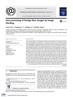
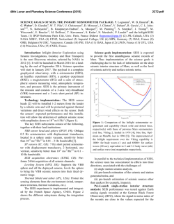
© Copyright 2026