
Advancing a Multimodal Transportation System by Eliminating
Advancing a Multimodal
Transportation System by
Eliminating Funding Restrictions
By Kevin DeGood and Andrew Schwartz January 2015
W W W.AMERICANPROGRESS.ORG
Advancing a Multimodal
Transportation System
by Eliminating Funding
Restrictions
By Kevin DeGood and Andrew Schwartz January 2015
Contents
1 Introduction and summary
6 Need for multimodal investments and flexibility
11 Multimodal best practices
17 Diminishing productivity and poor fiscal performance
from highways
22 Research results and methodology
37 State case studies
37 Texas
40 Arizona
43 Colorado
46 Georgia
49 Indiana
52 Minnesota
55 Missouri
58 Montana
61 Ohio
64 Tennessee
67 Washington
70 Wyoming
73 Conclusion
74 About the authors
75 Endnotes
Introduction and summary
Most of our assumptions have outlived their uselessness.–Marshall McLuhan1
One of the most pervasive, durable, and detrimental myths in transportation policy
is that highways pay for themselves, while public transportation does not. In reality,
both modes require significant public subsidies, as user fees—such as fuel taxes
and farebox revenues—cover only a portion of total costs. States and the federal
government supplement these user fees with property taxes, bonding, and general
revenues. On average, these nonuser fee revenues represent 26 percent of total
annual highway expenditures.2
Moreover, treating all highways equally obscures the fact that per-mile construction
and maintenance costs, driving levels, and motor fuel tax revenues vary substantially
depending on the location, size, and population around a particular road. While the
overwhelming majority of driving occurs within metropolitan areas, many large
urban highways and arterial roads cost substantially more money to maintain than
they generate in fuel taxes. This is also true of many rural and exurban arterial roads.
This means that states must cross subsidize thousands of miles of roads that generate
insufficient gas tax revenues each year.
Research by the Center for American Progress shows that nearly 4 in 10 miles of
interstate highway and other principal arterial roadways fail to generate enough in
user fees to cover their long-term maintenance costs. For the purposes of this analysis,
maintenance costs include one reconstruction and multiple resurfacings over the
course of three decades while excluding the costs of land acquisition, engineering,
construction, and inflation.
When the analysis is conducted assuming 1 percent annual inflation, the share of
interstate and other principal arterial roadways that fail to cover their costs rises by
more than 22,000 miles, or 9 percent. In all likelihood, actual construction inflation
will be much higher than 1 percent per year over the next 30 years. Furthermore, if
land acquisition and construction expenses were amortized over the same period,
an even higher share of roadways would fail to cover their costs.
1 Center for American Progress | Advancing a Multimodal Transportation System by Eliminating Funding Restrictions
This research also strongly suggests that an even higher share of minor arterial
roadways, collectors, and other local roads fail to cover their long-term costs. A
disproportionately large percentage of driving occurs on interstates and principal
arterials—which make up the National Highway System, or NHS—relative to the
rest of the roadway network. Data from the U.S. Department of Transportation’s
Federal Highway Administration shows that the NHS accounts for only 5.5 percent
of all roadway miles yet carries 55 percent of all vehicle miles traveled, or VMT,
each year.3 As a result, the remaining 94 percent of the system generates much less
user fee revenue on a per-mile basis, since it carries less than half of all driving.
TABLE 1
Fiscal performance of interstates and principal arterials
Geography
Loss
Share
Breakeven
Share
Surplus
Share
Urban areas, more than 1 million residents
5,340
44%
2,054
17%
4,643
39%
Urban areas, between 200,000 and 1 million residents
6,125
23%
3,973
15%
17,027
63%
Urban areas, between 50,000 and 200,000 residents
43,286
47%
11,178
12%
37,893
41%
Urban subtotal
54,752
42%
17,205
13%
59,564
45%
Rural subtotal
34,979
35%
10,764
11%
55,338
55%
National total
89,731
39%
27,968
12%
114,903
49%
Source: Based on authors’ calculations from the Federal Highway Administration, “HPMS Public Release of Geospatial Data in Shapefile Format,” available at http://www.fhwa.dot.gov/
policyinformation/hpms/shapefiles.cfm (last accessed October 2014); Federal Highway Administration, “2013 Status of the Nation’s Highways, Bridges, and Transit: Conditions &
Performance,” available at http://www.fhwa.dot.gov/policy/2013cpr/appendixa.htm (last accessed October 2014); U.S. Energy Information Administration, Petroleum Marketing
Monthly May 2014 (U.S. Department of Energy, 2014), available at http://www.eia.gov/petroleum/marketing/monthly/pdf/mgt.pdf; Federal Highway Administration, State MotorFuel Taxes and Related Receipts - 2012 (1) (U.S. Department of Transportation, 2013), available at http://www.fhwa.dot.gov/policyinformation/statistics/2012/pdf/mf1.pdf; Federal
Highway Administration, Revenues Used By States for Highways - 2012 1/ (U.S. Department of Transportation, 2013), available at http://www.fhwa.dot.gov/policyinformation/
statistics/2012/pdf/sf1.pdf.
TABLE 2
Fiscal performance of interstates and principal arterials including inflation
Geography
Loss
Share
Breakeven
Share
Surplus
Share
Urban areas, more than 1 million residents
7,672
64%
1,750
15%
2,616
22%
Urban areas, between 200,000 and 1 million residents
9,295
34%
5,366
20%
12,463
46%
Urban areas, between 50,000 and 200,000 residents
50,816
55%
11,353
12%
30,190
33%
Urban subtotal
67,783
51%
18,469
14%
45,269
34%
Rural subtotal
44,523
44%
11,722
12%
44,836
44%
National total
112,306
48%
30,191
13%
90,105
39%
Source: Based on authors’ calculations from the Federal Highway Administration, “HPMS Public Release of Geospatial Data in Shapefile Format,” available at http://www.fhwa.dot.gov/
policyinformation/hpms/shapefiles.cfm (last accessed October 2014); Federal Highway Administration, “2013 Status of the Nation’s Highways, Bridges, and Transit: Conditions &
Performance,” available at http://www.fhwa.dot.gov/policy/2013cpr/appendixa.htm (last accessed October 2014); U.S. Energy Information Administration, Petroleum Marketing
Monthly May 2014 (U.S. Department of Energy, 2014), available at http://www.eia.gov/petroleum/marketing/monthly/pdf/mgt.pdf; Federal Highway Administration, State MotorFuel Taxes and Related Receipts - 2012 (1) (U.S. Department of Transportation, 2013), available at http://www.fhwa.dot.gov/policyinformation/statistics/2012/pdf/mf1.pdf; Federal
Highway Administration, Revenues Used By States for Highways - 2012 1/ (U.S. Department of Transportation, 2013), available at http://www.fhwa.dot.gov/policyinformation/
statistics/2012/pdf/sf1.pdf.
2 Center for American Progress | Advancing a Multimodal Transportation System by Eliminating Funding Restrictions
States and the federal government fund a substantial portion of their transportation
expenditures by taxing the sale of gasoline and diesel fuel. Highway proponents have
successfully enacted prohibitions against using fuel tax revenues to support public
transportation and other multimodal projects in 30 states.4 At the federal level, there
is an unofficial rule that no more than 20 percent of fuel tax revenue can support
public transportation, also referred to as transit.5 These prohibitions and unofficial
limits hamper the ability of states and metropolitan regions to effectively plan for
future needs, as many worthwhile transit and multimodal projects languish due to
a lack of funds.
Highway boosters have exploited the myth of self-sufficiency to argue that fuel
tax revenue should only fund highway and bridge projects. In effect, highway
boosters argue that the source of the money should determine what that money
builds. This approach misses that, in many urban areas, transit, passenger rail, or
other multimodal projects are the most effective means of achieving an efficient,
economically productive, equitable, and environmentally sustainable transportation
system. While a roadway may produce an important share of transportation tax
revenues, additional roadway construction may not be the most appropriate
mobility solution. In short, objective measures of transportation system needs
should determine transportation priorities regardless of the source of funds.
In addition to the myth of highway user fee self-sufficiency, funding restrictions are
predicated on the false notion that public transportation riders do not pay gas taxes
and therefore do not pay into the system. The primary issue is the assumption that
people who ride transit never drive. In fact, the vast majority of transit riders does
indeed drive and, as a result, pays motor fuel taxes. A recent national survey by the
American Public Transportation Association found that 82 percent of transit riders
live in a household with a car.6 Of those transit riders with access to a car, 87 percent
used the vehicle more than three times per week.7 As this research shows, driving
and public transportation are complementary, with residents paying into the system
that allows them the flexibility to choose the mode of transportation that meets
their needs for any given trip.
Objective measures
of transportation
system needs
should determine
transportation
priorities regardless
of the source of
funds.
3 Center for American Progress | Advancing a Multimodal Transportation System by Eliminating Funding Restrictions
Beyond the issue of funding, transit provides significant benefits for people who
exclusively drive, as public transportation lowers roadway congestion.8 In the absence
of transit service, riders would be forced to drive for all trips, adding vehicles to the
network during the peak periods of travel demand—the morning and the evening.
Research by Texas A&M University shows that if transit services were stopped in the
top 10 largest metropolitan regions, it would increase roadway delay by 677 million
hours each year.9 Yet prohibitions on the use of gas taxes to fund public transit mean
that metropolitan and state transportation authorities are often denied the ability to
implement a balanced surface transportation system capable of delivering the most
benefits to residents and businesses.
The negative consequences of funding restrictions are especially harmful in metropolitan areas with growing roadway congestion. Research shows that total hours
of roadway delay in urban areas increased by 400 percent from 1982 to 2011.10
Yet state and local planners are often prevented from using user fee revenues,
overwhelmingly generated by urban drivers, to improve the transportation system
through balanced investment.
Data from the Federal Highway Administration show that 67 percent of all VMT—
or 1.9 trillion miles annually—occurs within urban areas.11 Urban drivers generate
nearly $7 out of every $10 in user fees, but they face counterproductive restrictions
regarding how those funds may be used. States and metropolitan regions should
have the flexibility to implement needed transportation projects regardless of the
source of funding.
TABLE 3
Annual hours of
additional roadway delay
if transit service ended
Metro region
Hours
New York
440,647,000
Chicago
67,432,000
Boston
37,943,000
Washington
33,810,000
Los Angeles
32,345,000
Philadelphia
30,167,000
Miami
11,589,000
Atlanta
10,520,000
Houston
6,733,000
Dallas-Fort Worth
6,292,000
Total
677,478,000
Source: David Schrank, Bill Eisele, and Tim Lomax,
“Urban Mobility Report 2012” (College Station, TX:
Texas A&M Transportation Institute, 2012), available
at http://d2dtl5nnlpfr0r.cloudfront.net/tti.tamu.edu/
documents/mobility-report-2012.pdf.
The U.S. surface transportation system is a complex mix of different modes, including
highways, intercity passenger rail, public transportation, freight rail, and intermodal
connections that allow freight to flow from ship to train and from train to truck.
Funding restrictions at the state and federal levels represent a major barrier to
successfully planning and implementing an efficient, equitable, sustainable, and
globally competitive transportation system.
Reforming surface transportation will require changes at the federal and state levels.
Specifically, Congress should establish a multimodal account within the Highway
Trust Fund to provide funding for highway, transit, passenger and freight rail,
port development, and intermodal facilities, among other projects. Funding from
this multimodal account should be distributed through a competitive program
administered by the Department of Transportation’s Office of the Secretary. In
addition, states should be given the flexibility to use any portion of their federal
highway funds for any project category eligible under the multimodal program.
4 Center for American Progress | Advancing a Multimodal Transportation System by Eliminating Funding Restrictions
At the state level, legislatures should repeal any statutory or state constitutional
prohibitions that prevent the use of motor fuel taxes or other user fees for projects
other than highways. Once these restrictions have been lifted, states should require
their respective transportation departments to engage in scenario planning based
upon achieving objectives and quantifiable system performance goals.
Taken together, increased funding flexibility from Congress and state legislatures
and goal-driven scenario planning will allow transportation agencies to implement
a truly multimodal, integrated, and balanced system.
5 Center for American Progress | Advancing a Multimodal Transportation System by Eliminating Funding Restrictions
Need for multimodal investments
and flexibility
Following the end of World War II, the U.S. economy and population expanded
rapidly. Yet existing highway infrastructure was inadequate to meet the need for
efficient long-distance travel and land development around cities. Originally, early
road funds from the federal government flowed through the U.S. Department of
Agriculture. Later, they flowed through the U.S. Department of Commerce.12 While
important, this modest funding did not represent a national investment program.
In 1956, then-President Dwight D. Eisenhower signed into law the Federal-Aid
Highway Act, which established the Highway Trust Fund and created a program
to build the interstate highway system.13 The initial focus of the federal surface
transportation program was highway development. The Federal-Aid Highway Act of
1956 and subsequent authorizations succeeded in providing seamless and efficient
connections between urban areas, while also supporting rural communities with
better farm-to-market roads.
However, the narrow focus of the program addressed only part of the country’s
transportation needs, leaving out mass transit and other multimodal priorities. In
1982, then-President Ronald Reagan signed into law the Surface Transportation
Assistance Act.14 The legislation expanded the mandate of the Highway Trust Fund
by establishing the Mass Transit Account to provide dedicated funding in support
of transit operation, as well as capital needs.15
The time has come to once again expand the mandate of the Highway Trust Fund
to include a third multimodal account to support surface transportation projects
currently excluded from the federal program, as well as major highway and transit
capital projects. The Surface Transportation Assistance Act of 1982 recognized
the shortcoming of only providing dedicated funding for highway construction
and maintenance. Similarly, a new multimodal account would recognize the
shortcoming of excluding freight and passenger rail, port development, and other
multimodal projects.
6 Center for American Progress | Advancing a Multimodal Transportation System by Eliminating Funding Restrictions
In addition to these excluded project categories, a new multimodal account should
support major highway and transit capital projects that are too large for a state or
metropolitan region to complete using annual formula funds. The core highway
and transit formula programs, which account for 95 percent of all federal surface
transportation outlays, are a vital source of funds to complete thousands of projects
each year.16 On average, states have more than 2,300 active highway and transit
projects receiving trust fund support at any given time.17 The vast majority of these
projects are modest in scope and cost. These projects are essential to the ongoing
maintenance and incremental improvement of our roadway and transit systems.
However, these funds are often inadequate to address larger capital needs. A single
large highway or transit project with regional or national significance could easily
consume a state’s entire allocation for multiple years, displacing thousands of
smaller projects as a result.
Defining the roadway network
The federal government measures the roadway system in terms of centerline miles and
lane miles. Centerline miles measure system length, and lane miles measure capacity by
multiplying the roadway length by the number of lanes in each direction. For instance,
a roadway that connects two cities 10 miles apart with four travel lanes in each direction
is said to have 10 centerline miles and 80 lane miles. This report presents data in terms
of centerline miles, and all shorthand references to “miles” denote centerline miles.
In addition, roadways are classified by their purpose and design characteristics.
Limited-access highways and other roadways designed to move vehicles at high speeds
are classified as major arterial roadways. Major arterials include the interstate highway
system, freeways and expressways, and other high-speed signalized roadways. These
facilities make up the National Highway System. This paper will use the terms “arterial
roadway” and “NHS” interchangeably to refer to all major arterial roads.
7 Center for American Progress | Advancing a Multimodal Transportation System by Eliminating Funding Restrictions
In many ways, a new multimodal program would function as a much larger version
of the Transportation Investment Generating Economic Recovery, or TIGER, grant
program. Created as part of the American Recovery and Reinvestment Act of 2009
and continued by Congress in subsequent years, the TIGER program functions as
a competitive grant program that supports surface transportation projects regardless
of mode. A multimodal account would provide funding for a competitive program
that would build on the best aspects of the TIGER program, with the added benefit
of providing dedicated funding not subject to annual appropriations. In short,
expanding the types of projects covered by the Highway Trust Fund would ensure
a truly comprehensive and balanced federal program capable of making the types
of investments needed to advance the nation’s 21st century economy.
Beyond providing grant funding for a competitive multimodal program, the next
surface transportation authorization bill should substantially expand the flexibility
of states and metropolitan regions to use their annual highway formula dollars as
they see fit. Currently, states and metropolitan regions have the flexibility to use
highway funds allocated under the Surface Transportation Program, or STP, for
either a roadway or transit capital projects. While beneficial, this practice continues
to limit the project selection decisions of states and regions. The flexibility should
be extended to any project eligible under the multimodal program. Under this
approach, a state or region could use its formula funds for surface transportation
projects, including passenger and freight rail, port access, and multimodal facilities,
among others.
Moreover, the STP represents only 26 percent of annual formula funds.18 The
expanded flexibility should also apply to the National Highway Performance
Program, or NHPP, and the Railway-Highway Crossing Program. Taken together,
these three programs account for more than 80 percent of formula funds, allowing
states both the flexibility and the dollar volumes necessary to make substantial
multimodal investments as needed.19
Finally, these funding reforms point to a more comprehensive role for the federal
government in surface transportation. The language used to describe that role is
important and should reflect the scope of the program. The Highway Trust Fund
received its name as part of the Federal-Aid Highway Act of 1956. At the time, the
name reflected the fact that the federal government made investments exclusively
focused on highways. Renaming the Highway Trust Fund the Transportation Trust
Fund would mirror the comprehensive nature of the restructured federal program.
8 Center for American Progress | Advancing a Multimodal Transportation System by Eliminating Funding Restrictions
Future growth and investment needs
Since the Highway Trust Fund was last reformed in 1982, the U.S. population has
grown by 76 percent, from 226 million to 315 million people.20 Over the next
50 years, the U.S. population will grow by approximately 100 million people.21
With this population growth will come more than 85 million additional commercial
and light-duty vehicles, increasing travel demand and stress on the transportation
system.22 Moreover, this travel demand will not be distributed evenly. In fact, growth
will overwhelmingly occur within metropolitan regions. More than 80 percent
of Americans live in urban areas, and urban populations are growing 25 percent
faster than rural populations.23
This has important implications for transportation policy because growing urban
congestion requires a broad mix of investments to efficiently move both people
and freight. The need for more transit, passenger and freight rail, and intermodal
projects reflects both the severe constraints facing highway expansion and economic
research that shows a precipitous decline in return on investment from additional
highway expansion. Initial highway investments following the Federal-Aid Highway
Act of 1956 and subsequent legislation produced substantial economic returns.
This productivity surge stemmed from the dramatic efficiency gains offered by major
highways compared with the existing roadway network. Yet further investments
have produced only marginal additional economic benefits, since the vast majority
of the efficiency gains have already been realized.24
Moreover, dense urban development patterns often make right-of-way acquisition
and property condemnation prohibitively expensive and politically challenging.
In the abstract, the American public often supports highway expansion. However,
this tentative support regularly switches to hostile opposition when the reality
of bulldozing homes and businesses becomes apparent. For this reason, highway
expansion tends to occur at the periphery of metropolitan regions where costs
and population densities are lower. Expansion on the periphery does little to nothing
to reduce economically damaging congestion in the rest of the region. These cost
and political realities are reflected by the fact that while the numbers of registered
vehicles and total miles driven have increased exponentially in recent decades, the
roadway network has only grown modestly.
9 Center for American Progress | Advancing a Multimodal Transportation System by Eliminating Funding Restrictions
TABLE 4
Changes in population, travel, and system capacity
1960
1980
2012
Percent change
1960–2012
Population
180 million
226.5 million
315 million
76%
Registered vehicles
74.4 million
161.5 million
253 million
240%
Vehicle miles traveled
718 billion
1.5 trillion
2.9 trillion
313%
Centerline miles
3.5 million
3.8 million
4.1 million
15%
-
7.9 million
8.6 million
8.6%
Lane miles
Source: Bureau of the Census, “Historical National Population Estimates: July 1, 1900 to July 1, 1999,” available at https://www.census.gov/
popest/data/national/totals/pre-1980/tables/popclockest.txt (last accessed October 2014); Bureau of the Census, Table 1. Monthly Population
Estimates for the United States: April 1, 2010 to November 1, 2013 (U.S. Department of Commerce, 2013), available at http://www.census.gov/
popest/data/state/totals/2012/tables/NA-EST2012-01.xls; Bureau of Transportation Statistics, Table 1-11: Number of U.S. Aircraft, Vehicles, Vessels,
and Other Conveyances (U.S. Department of Transportation), available at http://www.rita.dot.gov/bts/sites/rita.dot.gov.bts/files/table_01_11.
xlsx; Federal Highway Administration, Public Road Mileage - VMT - Lane Miles 1920 - 2012 (U.S. Department of Transportation, 2012), available at
http://www.fhwa.dot.gov/policyinformation/statistics/2012/xls/vmt421c.xls.
The lack of balanced investments combined with the rapid growth in travel demand
has dramatically increased congestion. Between 1982 and 2011, total hours of
roadway delay in urban areas increased by 400 percent.25 Each year, congestion
costs the economy $120 billion in lost productivity and wasted fuel.26 Continuing
to focus limited transportation funds disproportionately on highway investments
that provide marginal returns will only exacerbate this economic cost.27
This is especially troubling for the freight sector and for businesses that rely on
international trade, a global supply chain, and just-in-time delivery. As a share of
our gross domestic product, trade accounted for less than 10 percent of economic
activity in 1960.28 Today, trade accounts for more than 20 percent of economic
activity each year, or $3.2 trillion.29 This share will continue to rise in the coming
decades, as international freight shipments are projected to grow by 3.4 percent
each year.30 Research from the Federal Highway Administration shows that over
the next 30 years, truck freight will increase by 65 percent, reaching more than 18
billion tons annually.31
Business-as-usual transportation investments will not be sufficient to accommodate
and support this expected growth. States and the federal government must make
diverse investments to more efficiently, equitably, and sustainably move people
and goods.
10 Center for American Progress | Advancing a Multimodal Transportation System by Eliminating Funding Restrictions
Multimodal best practices
The lack of funding flexibility and the historic imbalance in the federal program
have left many beneficial transportation projects on the shelf to collect dust. The
following examples represent best practices and the kinds of projects that a
multimodal account and greater programmatic flexibility would fund.
Alameda Corridor
The ports of Los Angeles and Long Beach, California, make up the busiest port
complex in the United States, handling 14.5 million twenty-foot equivalent unit
containers, or TEUs, annually, with a value well in excess of $300 billion.32 The
port plays a significant role in the regional economy, accounting for 1 out of every
15 jobs in Southern California.33 Yet this economic productivity comes at a price.
The busy port complex generates a substantial amount of rail and truck traffic.
Prior to the completion of the Alameda Corridor, long freight trains traveling at
grade—meaning that they traveled on tracks that intersected with local streets—
caused lengthy delays to the roadway network dozens of times per day.34 In effect,
transportation bottlenecks exterior to the port threatened to limit its ability to grow
and remain competitive in the long term.
The Alameda Corridor is a 20-mile-long railroad trench that separates freight trains
from street traffic, linking the port complex to the transcontinental rail network near
downtown Los Angeles. The trench removed more than 200 at-grade crossings.35
Today, the corridor carriers a staggering 16,500 trains per year, dramatically reducing
roadway congestion, noise, and pollution from idling vehicles.36
11 Center for American Progress | Advancing a Multimodal Transportation System by Eliminating Funding Restrictions
The $2.4 billion project was financed through a combination of
$400 million in government grant funding and $2 billion in
revenue bonds to be repaid with container fees paid by the
railroads and collected by the Alameda Corridor Transportation
Authority. As of January 1, 2014, rail carriers must pay $22.58 for
each loaded TEU; $5.41 for each TEU returning empty; and
$10.82 for other types of rail cars, such as tankers.37 The project
involved 1,280 construction jobs for local residents, including
637 workers placed in union apprenticeships.38
Each day, the Alameda Corridor carries approximately 45 trains
and 13,000 TEUs.39 The congestion and environmental benefits
from the corridor project are substantial. A single train eliminates
the equivalent of between 250 and 280 trucks.40 This translates
into the removal of between 4.3 million and 4.9 million truck
trips from the port each year.41
Alameda Corridor Rail Trench
Alameda Corridor Connection with
Transcontinental Rail Yard
Hudson River tunnel
The Northeast Corridor rail line, which stretches from Boston,
Massachusetts, to Washington, D.C., is the busiest rail line in the
United States. One of the most critical and overburdened sections
is the Hudson River tunnels—also known as the North River
Tunnels—that connect New York City’s Lower Manhattan with
Jersey City, New Jersey. The tunnels are more than 100 years old
and in need of replacement. Recently, the CEO of Amtrak stated
that the existing tunnels have as little as 20 years of useful life
remaining before one or both will have to be shut down permanently.42 Losing one or both tunnels would have substantial negative
transportation and economic consequences. The tunnels operate
at capacity during the morning and evening peak periods, moving
23 trains through per hour.43 The timing of service is so tight that a
single 15-minute disruption can affect 15 commuter and passenger
rail trains.44
Photos courtesy of the Alameda Corridor Transportation Authority.
Beginning in the 1990s, planners studied more than 100 different project alternatives to determine the most effective way to meet future travel demand.45 The
analysis showed that the most effective solution was to construct two new tunnels
under the Hudson River to expand rail access between New York and New Jersey.
12 Center for American Progress | Advancing a Multimodal Transportation System by Eliminating Funding Restrictions
The new tunnels would more than double the number of trains per hour—
increasing capacity from 23 to 48—and eliminate more than 32,000 daily transfers.46 In addition, the expanded service would reduce commute times by an
average of 23 minutes. The new tunnels would also eliminate approximately
22,000 automobile trips and 590,000 miles of driving every day—a significant
benefit to drivers who already face heavily congested roadways.47 In short, the new
tunnels would provide the transportation access necessary to allow the region to
grow for decades to come.
Chicago freight rail
For nearly 150 years, the Chicago region has served as a hub for national freight
and passenger rail traffic. In fact, one-quarter of all freight rail traffic—37,500 rail
cars each day—flows through the Chicago region.48 The extensive rail network
suffers from bottlenecks and numerous conflict points with local roadways, causing
significant delays that add environmental pollution from idling vehicles and reduce
productivity. In fact, the average rail car requires almost 30 hours to travel through
the Chicago area.49
The Chicago Region Environmental and Transportation Efficiency program,
or CREATE, is a series of infrastructure improvements designed to considerably
improve freight and passenger rail travel times in the Chicago metropolitan area.
The program represents a unique partnership that includes the state of Illinois,
the city of Chicago, the commuter rail operator Metra, Amtrak, and the U.S.
Department of Transportation.50 The CREATE program consists of 70 projects,
including 25 road-rail grade separations; six rail-rail grade separations; and 36 other
improvements to tracks, switches, and signal systems.
Once the CREATE program is completed, area residents will save approximately
3,800 hours each day—hours they currently spend idling as trains pass.51 The
improved efficiency for freight trains and the reduced wait times for trucks will save
3.4 million gallons of diesel fuel each year.52 This includes reductions of 36,000
metric tons of carbon dioxide, 155 metric tons of nitrogen oxide, and 5 metric tons
of particulate matter.53 Finally, the Chicago region relies heavily on commuter rail
and passenger rail operations, with Metra serving 36 million riders and Amtrak
serving more than 2.6 million. The CREATE program will reduce total annual delay
for Metra and Amtrak riders by a projected 817,000 hours.54
13 Center for American Progress | Advancing a Multimodal Transportation System by Eliminating Funding Restrictions
CREATE Program Project Map
Rendering courtesy of the Chicago Department of Transportation.
The CREATE program has a total estimated cost of $3.8 billion.55 To date, the
program has received $1.2 billion, with 22 projects waiting for funding.56 Yet this
incredibly important program of projects has received only $339 million in federal
funds, with the largest share coming from a one-time infusion through the American
Recovery and Reinvestment Act.57
14 Center for American Progress | Advancing a Multimodal Transportation System by Eliminating Funding Restrictions
North Carolina passenger rail
Over the next 20 years, North Carolina’s population is anticipated to grow by 52
percent, which is the seventh-fastest population growth in the nation.58 Much of
this growth will occur within the Piedmont region, which extends from Charlotte
to the Raleigh-Durham-Chapel Hill Triangle region. This growth will substantially
increase intercity travel demand and highway congestion.
Piedmont Improvement Program Project Map
Rendering courtesy of the North Carolina Department of Transportation.
North Carolina is unique in that it owns 317 miles of railroad track with a 200-foot
wide right of way extending from Charlotte through the Triangle region to Morehead
City on the coast. For years, Amtrak has offered two daily round trips between
Raleigh and Charlotte as part of its Piedmont and Carolinian lines. In addition to
passenger service, Norfolk Southern and CSX Transportation use the track to provide
freight rail operations.
15 Center for American Progress | Advancing a Multimodal Transportation System by Eliminating Funding Restrictions
As far back as the 1990s, the state initiated planning to expand passenger rail
service along the Piedmont corridor. The project became known as the Piedmont
Improvement Program, or PIP. PIP consists of a series of infrastructure improvements that will increase passenger rail service from two to five round trips each day.59
The program includes adding 13 new bridges and removing 23 rail crossings to
separate vehicle and rail traffic in order to reduce accidents and improve overall
travel times.60 In addition, the program involves adding 32 miles of additional track
to allow passing zones for passenger trains traveling at higher speeds than freight
traffic. State traffic modeling shows that the expanded rail service will remove
66,000 automobile trips and 8 million miles of driving between Charlotte and
Raleigh each year.61 In 2013, the corridor carried a total of 363,000 passengers.62
The Piedmont project is primarily supported by $520 million in one-time funding
from American Recovery and Reinvestment Act.63 In total, the Federal Railroad
Administration received grant requests for seven times more funding than was
available.64 The overwhelming response by states to the availability of American
Recovery and Reinvestment Act funds highlights the pent-up demand for federal
investment in rail. Yet now that the Federal Railroad Administration has distributed
these one-time funds, states and metropolitan regions are once again faced with a
federal transportation program that does not provide ongoing rail capital projects.
16 Center for American Progress | Advancing a Multimodal Transportation System by Eliminating Funding Restrictions
Diminishing productivity and poor
fiscal performance from highways
Highways are an essential part of our surface transportation system. The 4.1
million miles of public roadway in the United States form a comprehensive
national network that links our largest urban centers with our most rural communities.65 In fact, the size and extent of the system creates a network effect whereby
the economic utility of the system is greater than any one part. Yet the initial
productivity gains that resulted from investments following World War II have
given way to substantially lower returns in recent decades.
Research indicates that the net economic benefit of highway investments has fallen
by more than 70 percent from its peak after World War II.66 For example, one study
showed that highway expenditures added approximately 1.4 percent per year to
economic growth prior to the mid-1970s but have added only 0.4 percent per year
since.67 These results highlight a fundamental truth: Making incremental improvements to a transportation network are never as productive as the initial construction.68
The arguments in support of transportation policies that disproportionately
favor highway investments over other modes are further diminished when fiscal
performance and congestion are added to the analysis. While total driving levels
have risen substantially in the past 40 years—especially within urban areas—
this increase has not resulted in positive fiscal performance for many roadways,
even in the largest metropolitan regions.
Texas is a state known for driving, and it provides a powerful example of the paradox
of rising congestion and poor roadway fiscal performance. Texas has 3,961 arterial
miles in its five largest metropolitan regions—Houston, Dallas-Fort Worth,
San Antonio, Austin, and El Paso. Of this total, 73 percent of these roadways have
insufficient vehicle traffic to generate enough gas tax revenue to cover long-term
maintenance costs. At the same time, research by Texas A&M University shows there
were almost 408 million hours of delay in 2011 due to congestion in the same five
metropolitan areas.69
17 Center for American Progress | Advancing a Multimodal Transportation System by Eliminating Funding Restrictions
TABLE 5
Rising congestion in five largest Texas metro regions, 1982–2011
Increase in total delay
Increase in congestion
cost per driver
Increase arterial
roadway lane miles
Houston
339%
292%
136%
Dallas-Fort Worth
1335%
897%
84%
San Antonio
1243%
1212%
69%
Austin
1073%
579%
181%
El Paso
1061%
1066%
72%
Metro area
Source: Results based on authors’ calculation from Texas A&M University, “Complete Data” (2012), available at http://tti.tamu.edu/documents/
ums/congestion-data/complete-data.xls.
Increased driving and poor fiscal performance may seem counterintuitive. After all,
how can metropolitan areas have both increased congestion and facilities that cost
far more to build and maintain then they generate in user fees from gas taxes?
The answer is twofold: First, travel demand is not distributed uniformly throughout
the day. The morning and evening rush hours can easily overwhelm a highway or
arterial roadway, causing substantial delays and lost productivity. Yet that same
facility may be significantly underutilized throughout the rest of the day. As a result,
highways can be both congested and a serious fiscal burden.
Second, building and maintaining major highways and arterial roadways in urban
areas is expensive. Land acquisition, construction, and maintenance costs are far
greater in urban areas than in rural areas. On average, 1 mile of urban interstate costs
between 6 and 23 times more than 1 mile of rural interstate.70 And while low-density
suburban and exurban land-use patterns push people to drive slightly more than their
rural- or urban-core counterparts, the additional driving is not enough to offset the
added cost of these facilities. According to the Texas Department of Transportation,
the agency needs a staggering $5 billion more each year just to maintain congestion
levels as they currently stand.71
18 Center for American Progress | Advancing a Multimodal Transportation System by Eliminating Funding Restrictions
Scenario planning
In addition to removing funding restrictions and providing greater programmatic
flexibility, states and regions must reform how they engage in transportation planning.
Contemporary transportation planning is dominated by a focus on incremental
improvements in the absence of a compelling vision of how investments will produce
change in the future. All too often, future growth and land-use patterns are taken
as fixed, without regard for how transportation shapes where and what developers
build. Under this approach, investments take on a certain air of inevitability. Past
investment decisions extend into the future and produce more of the same results.
Scenario planning represents a dynamic approach to planning that discards the
idea that the future is predetermined and instead looks at how different bundles of
investments could shape future growth around economic, social, and environmental
goals. Rather than starting with a narrow review of existing transportation assets
and lists of project requests from local communities, scenario planning asks more
fundamental questions about what a community should look like 10, 20, or 30 years
in the future and then works backward to find the appropriate mix of projects to
achieve that vision. After all, transportation infrastructure has a profound effect on
the built environment and how people move through it.
One of the most important benefits of scenario planning is that it shifts the transportation conversation away from a debate over one project versus another and instead
asks a community to define its goals and values. These goals may include improved
safety or more affordable and equitable access to community amenities such as
health care, parks, schools, and job training. In effect, through scenario planning,
a community is able to express how transportation should facilitate and help
accomplish larger social, economic, and environmental goals.
Typically, scenario planning involves a consideration of multiple alternative investment approaches and a look at how these approaches would shape the community
in the coming years. Detailed transportation planning involves thousands of projects
over a long period of time. Understandably, this is more than most people care to
follow or try to understand. Scenarios cut through this complexity by focusing on
the ultimate outcomes rather than the process along the way.
19 Center for American Progress | Advancing a Multimodal Transportation System by Eliminating Funding Restrictions
Scenario planning is also beneficial because it does not look at transportation
investments through the lens of a particular mode of transportation. Once planners
have worked with the community to set clear goals, the task becomes finding the best
mix of investments to achieve those goals. Instead of allowing the source of money to
determine project selection, planners allow the performance characteristics of each
mode and potential project to drive the process. This rational approach to planning
recognizes that transportation is not its own end but rather a means to other ends.
Policy recommendations
The U.S. surface transportation system is a complex mix of different modes,
including highways, intercity passenger rail, public transportation, freight rail, and
intermodal connections that allow freight to flow from ship to train and from train
to truck. State and federal funding restrictions are a major barrier to successfully
planning and implementing a transportation system that is efficient, equitable,
sustainable, and globally competitive.
Additional information on
scenario planning is available
from the following publications: FHWA Scenario
Planning Guidebook,
available at http://www.fhwa.
dot.gov/planning/scenario_
and_visualization/scenario_
planning/scenario_planning_
guidebook/guidebook.pdf
and Building a 21st Century
Infrastructure, available at
http://www.americanprogress.org/issues/
economy/report/2014/02/12/84015/
building-a-21st-centuryinfrastructure/
With the current federal surface transportation authorization measure—Moving
Ahead for Progress in the 21st Century, or MAP-21—set to expire in May 2015,
Congress should take the following steps to increase programmatic flexibility and
invest in multimodal projects as part of the next authorization:
• Establish a multimodal account within the Highway Trust Fund to provide
funding for highway, transit, passenger and freight rail, port development, and
intermodal facilities, among other projects.
• Allocate multimodal funds through a competitive program administered by the
Department of Transportation’s Office of the Secretary.
• Allow states to flex any portion of their federal highway funds for any project
category eligible under the multimodal program.
• Rename the Highway Trust Fund the Transportation Trust Fund to reflect its
broad surface transportation mandate.
20 Center for American Progress | Advancing a Multimodal Transportation System by Eliminating Funding Restrictions
At the state level, legislatures should substantially increase the flexibility of
transportation departments to plan and implement a truly integrated and balanced
system by removing funding barriers:
• Repeal any statutory or state constitutional prohibitions on using motor fuel taxes
or other user fees for projects other than highways.
• Require state departments of transportation to set objective system performance
goals and to evaluate multiple projects and modes to determine which investments
will most cost effectively achieve those goals.
Taken together, these policy changes will allow limited transportation funding to
flow to the projects that produce the greatest improvement to overall system
performance and that deliver the most economic, social, and environmental benefits.
Yet removing funding restrictions is only part of the challenge. Decades of funding
silos have created planning silos. Beyond funding flexibility, states must reform their
planning processes to set objective economic, social, and environmental goals.
These goals should be independent of any one transportation mode or funding
source. With these goals in hand, state transportation departments must learn to
evaluate different investment scenarios that include multiple modes to determine
which project mix will be most cost effective.
21 Center for American Progress | Advancing a Multimodal Transportation System by Eliminating Funding Restrictions
Research results and methodology
This report presents an analysis of the fiscal performance of principal arterial
roadways, which also make up the National Highway System. Fiscal performance
is calculated by comparing the daily gas tax revenue generated by drivers on each
individual roadway with the daily cost to maintain that road. While the NHS
represents only 5.5 percent of all roadway miles, it carriers 55 percent of all vehicle
miles traveled.72 For this reason, the NHS will have the highest fiscal performance
of any roadway classification. Stated differently, the NHS represents the high-water
mark for fiscal performance, since the remainder of the roadway system carries much
less traffic per mile but has a similar cost profile.
The methodology used to conduct this analysis makes four assumptions intended
to yield the most favorable results for the NHS. First, the life cycle cost estimates
do not include right-of-way acquisition, engineering, or initial construction. This
lowers the total cost over the 30-year period and reduces the amount of driving a
roadway requires to break even or generate a surplus.
Second, the analysis assumes that gas tax revenues for light- and heavy-duty vehicles
will remain constant in the future. Rising vehicle efficiency standards have already
eroded the revenue-generating capacity of state and federal gas taxes. And while some
legislatures have increased gas taxes, these raises have not kept pace with efficiency
gains. For instance, Congress has not raised the federal gas tax since 1993.73 This
methodological choice also reduces the amount of driving needed for a roadway
to break even or generate a surplus.
Third, this analysis adjusts the life cycle cost estimate for each roadway down to
reflect the share of roadway expenditures covered by user fees. States fund their
roadway investments with revenues from multiple sources. As a result, user fees in
the form of gas taxes and tolls cover only a portion of the annual total. Fiscal
performance calculations reflect this reality by multiplying the life cycle cost estimate
by the share of roadway expenditures covered by user fees. For instance, if a state
derives 75 percent of its highway funding from user fees, the life cycle cost estimate
22 Center for American Progress | Advancing a Multimodal Transportation System by Eliminating Funding Restrictions
would be reduced by 25 percent. By adjusting the life cycle cost downward, the
analysis remains neutral about how a state chooses to fund its roadways. In effect,
this downward adjustment means that roadways are only being held accountable for
the share of life cycle costs intended to be covered by user fees. Again, this reduces
the amount of driving needed for a roadway to break even or generate a surplus.
Fourth, this analysis uses a 30 percent range for break-even calculations. This means
that the break-even driving level is adjusted up and down by 15 percent to create a
generous break-even range. Even though the life cycle cost estimates from the Federal
Highway Administration already reflect a national sample of high- and low-cost areas,
adding the 30 percent range around the break-even point ensures that borderline
roadways are treated as breaking even.
Results
Even with four methodological choices intended to yield favorable results for
highways, 39 percent of all NHS miles fail to generate enough user fee revenues to
cover their long-term maintenance costs. When moderate inflation of 1 percent
per year is added to the analysis, the share of NHS miles that lose money jumps to
48 percent. Given historic inflation patterns in the construction industry, this rate
is likely substantially lower than what the actual rate will be. With a higher inflation
target, the share of underperforming arterials would rise even higher. The following
tables present national summary data for both the noninflation and inflation
scenarios, as well as the results by state if no inflation is assumed.
TABLE 6
Fiscal performance of interstates and principal arterials
Geography
Loss
Share
Breakeven
Share
Surplus
Share
Urban areas, more than 1 million residents
5,340
44%
2,054
17%
4,643
39%
Urban areas, between 200,000 and 1 million residents
6,125
23%
3,973
15%
17,027
63%
Urban areas, between 50,000 and 200,000 residents
43,286
47%
11,178
12%
37,893
41%
Urban subtotal
54,752
42%
17,205
13%
59,564
45%
Rural subtotal
34,979
35%
10,764
11%
55,338
55%
National total
89,731
39%
27,968
12%
114,903
49%
Source: Based on authors’ calculations from the Federal Highway Administration, “HPMS Public Release of Geospatial Data in Shapefile Format,” available at http://www.fhwa.dot.gov/
policyinformation/hpms/shapefiles.cfm (last accessed October 2014); Federal Highway Administration, “2013 Status of the Nation’s Highways, Bridges, and Transit: Conditions &
Performance,” available at http://www.fhwa.dot.gov/policy/2013cpr/appendixa.htm (last accessed October 2014); U.S. Energy Information Administration, Petroleum Marketing
Monthly May 2014 (U.S. Department of Energy, 2014), available at http://www.eia.gov/petroleum/marketing/monthly/pdf/mgt.pdf; Federal Highway Administration, State MotorFuel Taxes and Related Receipts - 2012 (1) (U.S. Department of Transportation, 2013), available at http://www.fhwa.dot.gov/policyinformation/statistics/2012/pdf/mf1.pdf; Federal
Highway Administration, Revenues Used By States for Highways - 2012 1/ (U.S. Department of Transportation, 2013), available at http://www.fhwa.dot.gov/policyinformation/
statistics/2012/pdf/sf1.pdf.
23 Center for American Progress | Advancing a Multimodal Transportation System by Eliminating Funding Restrictions
TABLE 7
Fiscal performance of interstates and principal arterials including inflation
Geography
Loss
Share
Breakeven
Share
Surplus
Share
Urban areas, more than 1 million residents
7,672
64%
1,750
15%
2,616
22%
Urban areas, between 200,000 and 1 million residents
9,295
34%
5,366
20%
12,463
46%
Urban areas, between 50,000 and 200,000 residents
50,816
55%
11,353
12%
30,190
33%
Urban subtotal
67,783
51%
18,469
14%
45,269
34%
Rural subtotal
44,523
44%
11,722
12%
44,836
44%
National total
112,306
48%
30,191
13%
90,105
39%
Source: Based on authors’ calculations from the Federal Highway Administration, “HPMS Public Release of Geospatial Data in Shapefile Format,” available at http://www.fhwa.dot.gov/
policyinformation/hpms/shapefiles.cfm (last accessed October 2014); Federal Highway Administration, “2013 Status of the Nation’s Highways, Bridges, and Transit: Conditions &
Performance,” available at http://www.fhwa.dot.gov/policy/2013cpr/appendixa.htm (last accessed October 2014); U.S. Energy Information Administration, Petroleum Marketing
Monthly May 2014 (U.S. Department of Energy, 2014), available at http://www.eia.gov/petroleum/marketing/monthly/pdf/mgt.pdf; Federal Highway Administration, State MotorFuel Taxes and Related Receipts - 2012 (1) (U.S. Department of Transportation, 2013), available at http://www.fhwa.dot.gov/policyinformation/statistics/2012/pdf/mf1.pdf; Federal
Highway Administration, Revenues Used By States for Highways - 2012 1/ (U.S. Department of Transportation, 2013), available at http://www.fhwa.dot.gov/policyinformation/
statistics/2012/pdf/sf1.pdf.
TABLE 8
Fiscal performance by state
State
Loss
Break even
Surplus
Alaska
89%
2%
9%
Arkansas
59%
14%
28%
Arizona
29%
12%
59%
California
20%
14%
66%
Colorado
42%
17%
41%
Connecticut
48%
4%
47%
District of Columbia
24%
19%
58%
Delaware
0%
0%
100%
Florida
9%
12%
79%
Georgia
38%
16%
47%
Hawaii
2%
2%
97%
Iowa
33%
22%
44%
Idaho
63%
13%
24%
Illinois
12%
14%
74%
Indiana
21%
14%
66%
Kansas
28%
18%
54%
Kentucky
11%
19%
71%
Louisiana
23%
13%
64%
Massachusetts
16%
17%
67%
Maryland
11%
8%
81%
24 Center for American Progress | Advancing a Multimodal Transportation System by Eliminating Funding Restrictions
State
Loss
Break even
Surplus
Maine
23%
13%
64%
Michigan
26%
14%
60%
Minnesota
34%
21%
45%
Missouri
46%
17%
36%
Mississippi
58%
16%
25%
Montana
91%
4%
6%
North Carolina
15%
13%
72%
North Dakota
83%
10%
7%
Nebraska
41%
16%
43%
New Hampshire
1%
4%
95%
New Jersey
0%
0%
99%
New Mexico
65%
11%
24%
Nevada
78%
4%
17%
New York
1%
2%
97%
Ohio
33%
16%
51%
Oklahoma
42%
14%
45%
Oregon
35%
11%
53%
Pennsylvania
11%
9%
80%
Rhode Island
40%
22%
38%
South Carolina
58%
12%
30%
South Dakota
94%
4%
2%
Tennessee
47%
15%
38%
Texas
47%
16%
37%
Utah
30%
13%
57%
Virginia
12%
11%
78%
Vermont
16%
12%
72%
Washington
11%
10%
79%
Wisconsin
26%
14%
59%
West Virginia
19%
12%
68%
Wyoming
84%
11%
6%
Source: Based on authors’ calculations from the Federal Highway Administration, “HPMS Public Release of Geospatial Data in Shapefile
Format,” available at http://www.fhwa.dot.gov/policyinformation/hpms/shapefiles.cfm (last accessed October 2014); Federal Highway
Administration, “2013 Status of the Nation’s Highways, Bridges, and Transit: Conditions & Performance,” available at http://www.fhwa.dot.
gov/policy/2013cpr/appendixa.htm (last accessed October 2014); U.S. Energy Information Administration, Petroleum Marketing Monthly
May 2014 (U.S. Department of Energy, 2014), available at http://www.eia.gov/petroleum/marketing/monthly/pdf/mgt.pdf; Federal Highway
Administration, State Motor-Fuel Taxes and Related Receipts - 2012 (1) (U.S. Department of Transportation, 2013), available at http://www.fhwa.
dot.gov/policyinformation/statistics/2012/pdf/mf1.pdf; Federal Highway Administration, Revenues Used By States for Highways - 2012 1/ (U.S.
Department of Transportation, 2013), available at http://www.fhwa.dot.gov/policyinformation/statistics/2012/pdf/sf1.pdf.
25 Center for American Progress | Advancing a Multimodal Transportation System by Eliminating Funding Restrictions
In order to understand this result, it helps first to review how states fund roadway
projects. In addition, this section reviews the process for calculating the fiscal
performance of NHS roadway segments. The next section presents fiscal performance
data for 12 case-study states. These states were chosen because they broadly represent
the regional, size, and population diversity of the United States.
Roadway funding
The United States has more than 4 million miles of public roadways.74 The funding
to build and maintain these facilities comes from a combination of sources, including
motor fuel taxes, tolling, vehicle registration fees, license fees, general governmental
revenues, and the proceeds from issuing debt in the form of bonds, among others.
These revenue sources may be grouped into two categories: user fees and nonuser
fees. A user fee is a tax levied on drivers that corresponds to how much they use the
roadway system. This means that the total amount of user fee taxes paid by drivers
is directly related to their annual mileage. By comparison, a nonuser fee is a tax
levied on drivers regardless of how much they use the roadway system.
All 50 states and the District of Columbia levy a tax on every gallon of gasoline and
diesel fuel sold within their respective borders. In addition, the federal government
levies a tax of 18.4 cents per gallon on gasoline and 24.4 cents per gallon on diesel.75
Motor fuel taxes are a user fee because additional driving increases fuel consumption
and, as a result, the amount of fuel taxes paid each year.
Annual vehicle registration charges are nonuser fees because the amount paid is
the same regardless of total driving. Often, registration fees are calculated as a
percentage of the current value of the vehicle. In this way, they function as a form
of property tax. Similarly, annual license charges are not user fees because obtaining
a license does not require either owning a car or driving.
Motor fuel taxes are the largest source of funding for highway construction and
maintenance.76 However, not all roadways carry the same amount of traffic or
generate the same level of fuel tax revenue. Roadways not only vary in how much
revenue they generate, but they also have substantially different life cycle costs, which
include both initial construction and ongoing maintenance. Life cycle costs vary
based on the size, geographic location, and type of roadway in question. State departments of transportation functionally classify all roadways according to their design
and purpose, paying particular attention to vehicle speed and land access. The
primary purpose of local streets is to provide land access. As a result, they carry fewer
cars and limit vehicle speeds. Local roads funnel cars onto collectors, which are
26 Center for American Progress | Advancing a Multimodal Transportation System by Eliminating Funding Restrictions
larger roads that offer increased travel speeds and less land access. In turn, collector
roads funnel traffic onto arterial roadways, which have much higher travel speeds.
Arterial roads include a wide range of facilities, from major commercial corridors
in urban areas to fully access-controlled highways and the interstate system.77
The Department of Transportation publishes a database with information on all
public roadways called the Highway Performance Monitoring System, or HPMS.78
Each roadway is broken up into small segments, typically between 0.1 and 1 mile
in length. For each segment, the database provides multiple roadway characteristics.
This analysis focuses on four characteristics: geography, functional classification,
average daily traffic count, and number of through lanes.79 The geography code
labels roadway segments as either urban or rural. The functional classification code
labels each segment as interstate, freeway, expressway, other principal arterial,
collector, or local. The average daily traffic count represents the number of vehicles
expected to travel along a road segment on a given day. The count includes all vehicles
in all lanes in both directions of a segment. The through-lanes code indicates the
total number of lanes per segment. Finally, each segment has a spatial reference
available as a shapefile, which allows each segment to be mapped. When combined
with other data from the Department of Transportation, these characteristics allow
for an estimate of daily maintenance cost and user fee revenue, which forms the
basis of the fiscal performance determination.
The Department of Transportation also publishes roadway cost information as part
of the annual “Status of the Nation’s Highways, Bridges, and Transit: Conditions
& Performance” report. The Department of Transportation derives its estimates
from taking a sample of actual project costs by improvement type, including
reconstruction and resurfacing. The estimates are broken out by roadway type
and geography to reflect the cost differences associated with these characteristics.
The four geographical categories are rural, small urbanized, large urbanized, and
major urbanized. Small-urbanized areas are those with a population between 50,000
and 200,000 people, large-urbanized areas are those with a population between
200,000 and 1 million people, and major-urbanized areas are those with a population
of more than 1 million people.
The Department of Transportation report also provides a cost estimate for small
urban areas that have a population of between 5,000 and 49,000 people. The cost
differences between small urban and small urbanized is less than 1 percent. In order
to simplify the analysis, all nonrural roadway segments within an area that has a
population of under 200,000 people are treated as small urbanized.
27 Center for American Progress | Advancing a Multimodal Transportation System by Eliminating Funding Restrictions
While the HPMS dataset labels roadway segments as urban and rural, this does not
provide enough information to label an urban segment as small, large, or major.
In order to ensure that each segment was assigned the appropriate cost, this analysis
added additional geographic information using data from the Bureau of the Census
on metropolitan statistical areas. A metropolitan statistical area, or MSA, is made up
of a central urbanized population center of at least 50,000 individuals, along with
the adjacent communities that have a high degree of integration with the central
area.80 For instance, if an interstate segment lies within an MSA with a population
of more than 1 million people, it is assigned the life cycle cost that corresponds to
interstates within major-urbanized areas. This process was repeated for every
roadway segment in the nation.
The following table presents the Department of Transportation’s cost estimates for
different types of roadway work. Based on feedback from state department of
transportation officials, this analysis assumes that interstate segments will require one
reconstruction and three resurfacings over the next 30-year period. Furthermore,
the analysis assumes that other principal arterial roadways will require one
reconstruction and two resurfacings. These estimates were used to determine the
total long-term maintenance cost for each roadway segment. This total was then
divided by the total number of days in 30 years to derive a daily cost.
TABLE 9
Typical costs per lane mile for roadway reconstruction and resurfacing
Reconstruct
Resurface
Full cost
per lane
Rural: other principal arterial
$737,000
$524,000
$1,261,000
Rural: interstate
$920,000
$981,000
$1,901,000
Small urbanized: other principal arterial
$1,368,000
$766,000
$2,134,000
Large urbanized: other principal arterial
$2,005,000
$962,000
$2,967,000
Major urbanized: other orincipal arterial
$4,009,000
$1,554,000
$5,563,000
Small urbanized: freeway, expressway, interstate
$1,605,000
$1,371,000
$2,976,000
Large urbanized: freeway, expressway, interstate
$2,626,000
$1,839,000
$4,465,000
Major urbanized: freeway, expressway, interstate
$5,253,000
$3,045,000
$8,298,000
Road category
Source: Federal Highway Administration, “2013 Status of the Nation’s Highways, Bridges, and Transit: Conditions & Performance,” available at
http://www.fhwa.dot.gov/policy/2013cpr/appendixa.htm (last accessed October 2014).
28 Center for American Progress | Advancing a Multimodal Transportation System by Eliminating Funding Restrictions
The following table presents data on gas and diesel tax rates by state, along with the
adjustment factors on both the cost and revenue sides of the fiscal performance
equation. As noted previously, states fund their roadway networks with revenues
from multiple sources. The column labeled “Highway expenditure adjustment factor”
indicates the share of roadway expenditures that come from user fees.81 This factor
is used to adjust the roadway cost estimate downward to reflect the share of that cost
that must be covered by user fees. Similarly, all states receive user fee revenues, but
not all of this money is directed to roadways. In many states, a portion of user fees
is diverted to cover other expenses such as highway patrol officer salaries or public
education. The column labeled “Revenue adjustment factor” indicates the share of
user fees dedicated to roadways. This factor represents a 10-year average to avoid
fluctuations from one-time transfers, especially in the wake of the Great Recession.
TABLE 10
Motor fuel taxes by state
State diesel
Combined state
and federal diesel
Highway
expenditure
adjustment factor
Revenue
adjustment factor
39.27
21.85
46.25
76%
100%
12.4
30.8
12.7
37.1
61%
96%
Arizona
19
37.4
27
51.4
42%
87%
Arkansas
21.8
40.2
22.8
47.2
73%
94%
California
52.89
71.29
49.58
73.98
48%
100%
Colorado
22
40.4
20.5
44.9
47%
94%
49.3
67.7
54.9
79.3
49%
67%
23
41.4
22
46.4
52%
90%
District of Columbia
23.5
41.9
23.5
47.9
48%
81%
Florida
36.02
54.42
32.37
56.77
56%
77%
Georgia
28.45
46.85
31.97
56.37
54%
83%
Hawaii
48.05
66.45
50.08
74.48
58%
92%
Idaho
25
43.4
25
49.4
63%
90%
Illinois
39.1
57.5
44.9
69.3
56%
87%
Indiana
40.81
59.21
51.29
75.69
65%
94%
Iowa
22
40.4
23.5
47.9
48%
96%
Kansas
25
43.4
27
51.4
51%
94%
Kentucky
30.1
48.5
27.1
51.5
56%
92%
Louisiana
20.01
38.41
20.01
44.41
59%
100%
Maine
30.01
48.41
31.21
55.61
73%
97%
State gas
Combined state
and federal gas
Alabama
20.87
Alaska
State
Connecticut
Delaware
29 Center for American Progress | Advancing a Multimodal Transportation System by Eliminating Funding Restrictions
State diesel
Combined state
and federal diesel
Highway
expenditure
adjustment factor
Revenue
adjustment factor
45.4
27.75
52.15
49%
50%
26.5
44.9
26.5
50.9
39%
61%
Michigan
41.39
59.79
39.81
64.21
56%
88%
Minnesota
28.6
47
28.6
53
52%
87%
Mississippi
18.38
36.78
18
42.4
77%
94%
Missouri
17.3
35.7
17.3
41.7
59%
98%
Montana
27.75
46.15
28.5
52.9
76%
74%
Nebraska
27.3
45.7
26.7
51.1
49%
97%
Nevada
33.15
51.55
28.56
52.96
65%
84%
New Hampshire
19.63
38.03
19.63
44.03
55%
91%
New Jersey
14.5
32.9
17.5
41.9
43%
51%
New Mexico
18.88
37.28
22.88
47.28
46%
72%
New York
49.86
68.26
50.39
74.79
51%
59%
North Carolina
37.75
56.15
37.75
62.15
61%
89%
North Dakota
23
41.4
23
47.4
73%
99%
Ohio
28
46.4
28
52.4
71%
96%
Oklahoma
17
35.4
14
38.4
53%
63%
Oregon
31.07
49.47
30.34
54.74
46%
80%
Pennsylvania
41.8
60.2
52.1
76.5
58%
80%
Rhode Island
33
51.4
33
57.4
57%
47%
South Carolina
16.75
35.15
16.75
41.15
78%
93%
South Dakota
22
40.4
24
48.4
75%
87%
21.4
39.8
18.4
42.8
73%
91%
Texas
20
38.4
20
44.4
47%
58%
Utah
24.5
42.9
24.5
48.9
38%
92%
Vermont
32.05
50.45
31
55.4
56%
74%
Virginia
17.28
35.68
26.08
50.48
43%
86%
Washington
37.5
55.9
37.5
61.9
48%
98%
West Virginia
35.7
54.1
35.7
60.1
70%
99%
Wisconsin
32.9
51.3
32.9
57.3
53%
80%
Wyoming
24
42.4
24
48.4
59%
66%
State gas
Combined state
and federal gas
27
Massachusetts
State
Maryland
Tennessee
Source: American Petrolium Institute, “State Motor Fuel Tax Rates Effective 4/1/2014” http://www.api.org/oil-and-natural-gas-overview/industry-economics/~/media/Files/Statistics/State-Motor-FuelExcise-Tax-Update-Oct-2014.pdf; Federal Highway Administration, “Revenues Used By States For Highways - 2012 1/,” available at http://www.fhwa.dot.gov/policyinformation/statistics/2012/sf1.cfm
(last accessed October 2014); Federal Highway Administration, “State Motor Fuel Taxes and Related Receipts – 2010 1/,” available at https://www.fhwa.dot.gov/policyinformation/statistics/2010/mf1.
cfm (last accessed October 2014).
30 Center for American Progress | Advancing a Multimodal Transportation System by Eliminating Funding Restrictions
Estimating segment revenue
Determining the fiscal performance of a given roadway segment begins with
calculating the amount of user fee revenue generated by drivers on a daily basis.
Calculating revenue requires several pieces of information, including vehicle counts,
average fuel economy, traffic composition, and segment length.
The HPMS dataset provides an average annual daily traffic count, or AADT. This
number represents the number of vehicles that can be expected to traverse a road
segment on any given day. The counts include all vehicles in all lanes in both
directions of a segment. The Federal Highway Administration extrapolates these
estimates based on actual vehicle traffic counts from numerous locations around
the country. The AADT forms the foundation of the revenue calculation.
The next step is to determine the average fuel economy of vehicles on the road.
Research by the Department of Transportation finds that light-duty vehicles—
including cars; sport utility vehicles, or SUVs; and noncommercial trucks—
average 23.6 miles per gallon.82 Heavy-duty vehicles have an average fuel economy
of 6 miles per gallon.83 Revenue per mile can be calculated by dividing the fuel tax
by the fuel economy.
Revenue per mile =
Per-gallon fuel tax
Fuel economy
The light- and heavy-duty per-mile revenue rates are combined into a blended rate
based on traffic composition. Data from the Federal Highway Administration shows
that trucks represent 10 percent of vehicle traffic on most classifications of arterial
roadways. The heavy-duty truck share rises to 13 percent on rural arterials and 24
percent on rural interstates.84
The next step is multiplying the per-mile revenue estimate by the length of the
segment. Since the estimate is on a per-mile basis, it must be adjusted to reflect
the segment length. The final step is to adjust the revenue estimate based on the
revenue adjustment factor for that state, which represents the share of user fee
revenues that actually support the roadway network. An example calculation will
help show this process. This example assumes a large urban interstate segment in
Wisconsin that is 1.2 miles long with 12,000 daily vehicles, four through lanes,
and a 9-to-1 light- to heavy-duty-vehicle traffic ratio.
31 Center for American Progress | Advancing a Multimodal Transportation System by Eliminating Funding Restrictions
In Wisconsin, the combined state and federal gas and diesel taxes are 51.3 and 57.3
cents per gallon, respectively. Given this tax rate, the average light-duty vehicle with
a fuel economy of 23.6 miles per gallon, or mpg, will generate 2.2 cents per mile in
gas tax revenues. At the same time, a heavy-duty truck with a fuel economy of 6
miles per gallon will generate 9.5 cents per mile.
Light–duty-vehicle revenue per mile =
Heavy–duty-vehicle revenue per mile =
$0.513
= $0.022
23.6 mpg
$0.573
6 mpg
= $0.095
These two different per-mile rates are then combined into a blended rate by
multiplying each by their share of traffic. With light-duty vehicles making up 90
percent of traffic on the urban interstate segment and heavy-duty vehicles making
up only 10 percent, the blended rate works out to 2.9 cents per mile.
Blended-per-mile revenue = ($0.022 × 90%) + ($0.095 × 10%) = $0.029
The resulting blended rate is multiplied by the segment length, since the example
segment is greater than 1 mile in length. This yields an adjusted blended rate of 3.5
cents, which is then multiplied by the number of daily vehicles. This yields a revenue
estimate of $417 per day.
Segment-length adjusted rate = ($0.029 × 1.2 miles) = $0.035
Initial revenue estimate = ($0.035 × 12,000 vehicles) = $417
The last step is to multiply the estimate by the revenue adjustment factor for
Wisconsin, which is 80 percent. Thus, the final revenue estimate for this segment
is $334 per day.
Final revenue estimate = ($417 × 80%) = $334
32 Center for American Progress | Advancing a Multimodal Transportation System by Eliminating Funding Restrictions
Estimating segment cost
The second step in determining fiscal performance is to calculate a daily segment
cost. Highways, like all forms of infrastructure, require maintenance. Unlike driving,
however, there are long periods of time between projects. This analysis amortizes
total maintenance costs over a 30-year period in order to have a daily value that
matches with daily revenues from driving. Maintenance can take many forms, and
this analysis focuses on repaving and reconstruction, which involves substantial
rebuilding of the roadway. The last step in the process is to adjust the total daily
cost downward to reflect the share of costs covered by user fees.
The Federal Highway Administration’s Highway Economic Requirement System,
or HERS, provides reconstruction and rehabilitation cost estimates on a per-lanemile basis for various road types and locations in 2010 dollars. Due to near-zero
inflation in recent years, costs were not updated to 2014 dollars.85 HERS provides
different estimates based on the location and type of highway facility. The estimates
for rural roads vary depending on the topography, with three categories: flat,
rolling, and mountainous terrain. Since the HPMS database does not include
topographical information, this analysis treats all rural segments as flat, which is
the lowest-cost category.
To appropriately categorize urban roadways, HPMS segment data
were combined with 2010 Census population data. All roadway
segments within a metropolitan statistical area of more than 1
million in population were categorized as major urban, an MSA
of between 200,000 and 1 million people was categorized as large
urban, and an MSA of between 50,000 and 200,000 people was
categorized as small urban. By combining these two datasets,
each segment was assigned the appropriate maintenance costs
given its size, location, and functional classification.
TABLE 11
Roadway categories
Rural: other principal arterial
Rural: interstate
Small urbanized: other orincipal arterial
Large urbanized: other principal arterial
Major urbanized: other orincipal arterial
Small urbanized: freeway, expressway, interstate
Large urbanized: freeway, expressway, interstate
Major urbanized: freeway, expressway, interstate
This analysis assumes that each interstate segment will require a
Source: Based on data from Federal Highway Administration, “2013 Status
of the Nation’s Highways, Bridges, and Transit: Conditions & Performance,”
repaving every 10 years, as well as one reconstruction, while
available at http://www.fhwa.dot.gov/policy/2013cpr/appendixa.htm (last
accessed October 2014).
principal arterials will require two repavings and one reconstruction. The Federal Highway Administration presents costs estimates
on a per-lane-mile basis. For this reason, the segment-cost calculation includes the
number of lanes as well as the segment length. The total cost is then divided by
10,950 days, which is the total number of days over the 30-year life cycle.
33 Center for American Progress | Advancing a Multimodal Transportation System by Eliminating Funding Restrictions
Interstate daily segment cost =
(1 reconstruction + 3 repavings) × lanes × segment length
10,950 days in life cycle
The last step in the cost calculation is to adjust the daily segment cost downward
to reflect the share of roadway costs that are covered by user fees. This adjustment
ensures that the fiscal performance determination only holds each roadway
accountable for the share of costs that user fees are intended to cover.
Final interstate daily segment cost = (Daily cost estimate × user-fee percentage)
Fiscal performance is determined by the ratio of daily segment revenue to daily
segment cost. Since every segment has a slightly different length, the break-even
analysis could not use a static or universal break-even number. The ratio indicates
whether a segment loses money, breaks even, or generates a surplus. Technically,
the break-even point would be a ratio of exactly 1. However, this analysis uses a
range of 15 percent above and below. The break-even ratio is 0.85-to-1.15.
Segment break–even ratio =
Daily segment revenue
Daily segment cost
The example of the large-urbanized interstate segment in Wisconsin would have a
daily cost estimate based on three repavings and one reconstruction, for four lanes
of through traffic over 1.2 miles.
Interstate daily cost =
($4,465,000 × 4) × 1.2
= $1,957
10,950 days
Downward cost adjustment = ($1,957 × 53%) = $1,037
Fiscal performance determination =
$334
= 0.32
$1,037
The ratio of $334 in daily revenue compared with a daily cost of $1,037 yields a
ratio of 0.32, which is substantially lower than the lower bound of the break-even
range of 0.85 to 1.15. Therefore, this segment fails to generate enough revenue to
cover its long-term maintenance costs.
34 Center for American Progress | Advancing a Multimodal Transportation System by Eliminating Funding Restrictions
Inflation adjustment
The national fiscal performance numbers that include inflation follow the same
calculation steps. The only difference is that the cost estimates have been inflated
before being plugged into the calculation. For interstates, this analysis assumes
that repavings occur every 10 years, with one reconstruction occurring in year 20.
For all other principal arterials, the analysis assumes a repaving every 15 years and
a reconstruction in year 20. These intervals are not intended to reflect the exact
timing of a maintenance plan for an arterial highway. In reality, a state department
of transportation must assess each segment of roadway to determine maintenance
needs. Many heavily traveled urban highways will require more frequent and
substantial work than is captured in this analysis, while other segments may require
less. This methodological choice is intended to sufficiently account for the fact
that maintenance is spread over the life of a facility. Again, exact timing will vary.
The inflation assumption included in the model is modest. Data from the past 10
years are historical outliers since they include the Great Recession. From the period
of 2003 to 2013, construction inflation in the transportation sector averaged
approximately 1 percent growth each year.86 This analysis uses a 1 percent annual
compound interest rate. As a result, the inflation coefficient for year 10 is 1.10;
it is 1.22 in year 20 and 1.35 in year 30. Taken together, these inflation coefficients
result in full cost per lane miles as follows.
TABLE 12
Inflation-adjusted roadway costs per lane mile
Reconstruction
Resurfacing
Full cost per
lane
$899,140
$961,540
$1,860,680
Rural: interstate
$1,122,400
$1,200,090
$2,322,490
Small urbanized: other principal arterial
$1,668,960
$1,405,610
$3,074,570
Large urbanized: other principal arterial
$2,446,100
$1,765,270
$4,211,370
Major urbanized: other principal arterial
$4,890,980
$2,851,590
$7,742,570
Small urbanized: freeway, expressway, interstate
$1,958,100
$1,677,190
$3,635,290
Large urbanized: freeway, expressway, interstate
$3,203,720
$2,249,710
$5,453,430
Major urbanized: freeway, expressway, interstate
$6,408,660
$3,725,050
$10,133,710
Road category
Rural: other principal arterial
Source: Based on authors’ calculation from Federal Highway Administration, “2013 Status of the Nation’s Highways, Bridges, and Transit:
Conditions & Performance,” available at http://www.fhwa.dot.gov/policy/2013cpr/appendixa.htm (last accessed October 2014); Federal
Highway Administration, “Construction Cost Trends For Highways 1/,” available at https://www.fhwa.dot.gov/policyinformation/nhcci/pt1.cfm
(last accessed October 2014).
35 Center for American Progress | Advancing a Multimodal Transportation System by Eliminating Funding Restrictions
It is important to note that prior to the recession, construction costs increased by
a total of 40 percent from 2003 to 2006. Thus, the 1 percent annual compound
interest rate constitutes a very conservative estimate. In all likelihood, inflation
will be substantially higher over the next 30 years. Even with this low inflation
assumption, however, the analysis shows that the share of roadways that fail to
generate enough revenue to cover their long-term costs rises by 9 percent when
compared with the baseline analysis.
36 Center for American Progress | Advancing a Multimodal Transportation System by Eliminating Funding Restrictions
State case studies
Texas
Texas is the second-largest state in terms of population and geographic size. It has
an estimated population of 26.4 million,87 with 15.7 million registered vehicles88
spread out over 261,000 square miles.89 The state includes 18,265 centerline miles
of interstate and principal arterial roadway—the most of any state.90 This works
out to 1,445 residents per centerline mile of arterial roadway.91 The combined state
and federal tax rate is 38.4 cents per gallon for gasoline and 44.4 cents per gallon
for diesel, which ranks 40th among all states.92 Even with a large population, the
combination of an extensive arterial network and a low gas tax rate means that 51
percent of Texas’ network fails to generate enough user fee revenue to cover its
long-term costs.
Texas fiscal performance of interstate and arterial roadways
Geography
Loss
Share
Breakeven
Share
Surplus
Share
Urban areas, more than 1 million residents
2,900
73%
411
10%
650
16%
Urban areas, between 200,000 and 1 million residents
615
61%
202
20%
197
19%
Urban areas, between 50,000 and 200,000 residents
751
49%
313
21%
462
30%
Urban subtotal
4,266
66%
927
14%
1,309
20%
Rural subtotal
5,002
43%
2,006
17%
4,756
40%
National total
9,268
51%
2,933
16%
6,065
33%
Source: Based on authors’ calculations from the Federal Highway Administration, “HPMS Public Release of Geospatial Data in Shapefile Format,” available at http://www.fhwa.dot.gov/
policyinformation/hpms/shapefiles.cfm (last accessed October 2014); Federal Highway Administration, “2013 Status of the Nation’s Highways, Bridges, and Transit: Conditions &
Performance,” available at http://www.fhwa.dot.gov/policy/2013cpr/appendixa.htm (last accessed October 2014); U.S. Energy Information Administration, Petroleum Marketing
Monthly May 2014 (U.S. Department of Energy, 2014), available at http://www.eia.gov/petroleum/marketing/monthly/pdf/mgt.pdf; Federal Highway Administration, State MotorFuel Taxes and Related Receipts - 2012 (1) (U.S. Department of Transportation, 2013), available at http://www.fhwa.dot.gov/policyinformation/statistics/2012/pdf/mf1.pdf; Federal
Highway Administration, Revenues Used By States for Highways - 2012 1/ (U.S. Department of Transportation, 2013), available at http://www.fhwa.dot.gov/policyinformation/
statistics/2012/pdf/sf1.pdf.
37 Center for American Progress | Advancing a Multimodal Transportation System by Eliminating Funding Restrictions
Texas arterial roadway fiscal performance
Substantial loss
Moderate loss
Breakeven
Moderate surplus
Substantial surplus
0
100
200 Miles
The Texas Triangle megaregion encompasses a significant portion of the state’s
population, as well as a large amount of Texas’ total vehicular travel. This area
includes Houston, Dallas-Fort Worth, and San Antonio, which are the three largest
metropolitan areas in the state. Together, they account for 58 percent of the registered
vehicles but less than 30 percent of highway miles in the state.93 Seventy-three
percent of the 3,961 arterial miles within urban areas that possess populations of
more than 1 million people do not generate sufficient vehicle traffic and gas tax
revenue to cover long-term maintenance costs. This highlights that, while urban
areas account for a substantial portion of all driving, the resulting revenue is not
enough to cover the high cost of maintaining large arterial roadways.
Most of the area west of the Texas Triangle is rural. With the exception of El Paso,
a few other urban areas, and portions of Interstate 20 and Interstate 40, a significant
percentage of these roads lose money. This result stems from the extent of the
highway system, low fuel taxes, and low population density in that part of the state.
38 Center for American Progress | Advancing a Multimodal Transportation System by Eliminating Funding Restrictions
Dallas-Fort Worth
0
5
10 Miles
Registered vehicles as a share of all vehicles in state
Houston
0
20 Miles
Central Texas
0
Low share
Moderate share
Intermediate share
Elevated share
High share
10
12.5
25 Miles
Substantial loss
Moderate loss
Breakeven
Moderate surplus
Substantial surplus
39 Center for American Progress | Advancing a Multimodal Transportation System by Eliminating Funding Restrictions
Arizona
Arizona is a rapidly growing state with an estimated population of 6.6 million people94
covering 113,000 square miles.95 Gas and diesel taxes are 37.4 cents per gallon and
51.4 cents per gallon, respectively.96 This ranks Arizona 43rd for gas tax and 26th for
diesel tax among all states. Phoenix and Tucson are Arizona’s two major metropolitan
areas, and together, they possess 80 percent of the state’s 4 million vehicles97 and a
little under half of the state’s 4,073 miles of interstate highways and principal arterial
roadways.98 This works out to 1,620 residents per centerline mile of arterial roadway.99
Overall, nearly 60 percent of Arizona’s interstate and arterial roadways generate
enough revenue to cover or exceed their long-term costs. This stems from the fact
that Arizona heavily supplements its roadway budget with nonuser fee revenues.
As a result, gas-tax receipts only need to cover a modest share of long-term costs.
The fiscal performance of arterial roadways in Arizona differs significantly between
urban and rural areas. In urban areas, 58 percent of arterial roadways fail to generate
sufficient revenue to cover costs, while only 12 percent of rural arterials do not.100
Arizona fiscal performance of interstate and arterial roadways
Geography
Loss
Share
Breakeven
Share
Surplus
Share
Urban areas, more than 1 million residents
812
74%
124
11%
157
14%
Urban areas, between 200,000 and 1 million residents
27
9%
40
14%
220
77%
Urban areas, between 50,000 and 200,000 residents
6
8%
8
11%
59
81%
Urban subtotal
845
58%
171
12%
435
30%
Rural subtotal
314
12%
323
13%
1,902
75%
National total
1,158
29%
494
12%
2,337
59%
Source: Based on authors’ calculations from the Federal Highway Administration, “HPMS Public Release of Geospatial Data in Shapefile Format,” available at http://www.fhwa.dot.gov/
policyinformation/hpms/shapefiles.cfm (last accessed October 2014); Federal Highway Administration, “2013 Status of the Nation’s Highways, Bridges, and Transit: Conditions &
Performance,” available at http://www.fhwa.dot.gov/policy/2013cpr/appendixa.htm (last accessed October 2014); U.S. Energy Information Administration, Petroleum Marketing
Monthly May 2014 (U.S. Department of Energy, 2014), available at http://www.eia.gov/petroleum/marketing/monthly/pdf/mgt.pdf; Federal Highway Administration, State MotorFuel Taxes and Related Receipts - 2012 (1) (U.S. Department of Transportation, 2013), available at http://www.fhwa.dot.gov/policyinformation/statistics/2012/pdf/mf1.pdf; Federal
Highway Administration, Revenues Used By States for Highways - 2012 1/ (U.S. Department of Transportation, 2013), available at http://www.fhwa.dot.gov/policyinformation/
statistics/2012/pdf/sf1.pdf.
40 Center for American Progress | Advancing a Multimodal Transportation System by Eliminating Funding Restrictions
Arizona arterial roadway fiscal performance
Substantial loss
Moderate loss
Breakeven
Moderate surplus
Substantial surplus
0
25
50 Miles
41 Center for American Progress | Advancing a Multimodal Transportation System by Eliminating Funding Restrictions
Phoenix
0
4.75
Tucson
9.5 Miles
Registered vehicles as a share of all vehicles in state
0
2.5
5 Miles
Substantial loss
Moderate loss
Breakeven
Moderate surplus
Substantial surplus
Low share
Moderate share
Intermediate share
Elevated share
High share
42 Center for American Progress | Advancing a Multimodal Transportation System by Eliminating Funding Restrictions
Colorado
Colorado has 5.3 million residents,101 3.7 million registered vehicles,102 and is the
eighth-largest state in the country at 103,641 square miles.103 The Denver, Colorado
Springs, and Boulder metropolitan areas have two-thirds of the state’s registered
vehicles104 and slightly more than one-third of Colorado’s 4,800 interstate and
principal arterial miles.105 Drivers in the three largest metropolitan regions lost a
total of 88 million hours to congestion delay in 2011.106
The state has the 34th-highest gas tax at 40.4 cents per gallon and the 41st-highest
diesel tax at 44.9 cents per gallon.107 Overall, 42 percent of interstate and principal
arterial roadways fail to generate enough revenue to cover long-term costs. Colorado
has 1,104 residents per centerline mile of arterial roadway.108 At the same time, 17
percent of arterial roadways break even, and 41 percent are generating surplus revenue.
Colorado fiscal performance of interstate and arterial roadways
Geography
Loss
Share
Breakeven
Share
Surplus
Share
Urban areas, more than 1 million residents
446
59%
137
18%
173
23%
Urban areas, between 200,000 and
1 million residents
97
29%
59
17%
179
53%
Urban areas, between 50,000 and
200,000 residents
80
25%
59
18%
185
57%
Urban subtotal
624
44%
254
18%
537
38%
Rural subtotal
1392
41%
563
17%
1429
42%
National total
2015
42%
817
17%
1967
41%
Source: Based on authors’ calculations from the Federal Highway Administration, “HPMS Public Release of Geospatial Data in Shapefile Format,” available at http://www.fhwa.dot.gov/
policyinformation/hpms/shapefiles.cfm (last accessed October 2014); Federal Highway Administration, “2013 Status of the Nation’s Highways, Bridges, and Transit: Conditions &
Performance,” available at http://www.fhwa.dot.gov/policy/2013cpr/appendixa.htm (last accessed October 2014); U.S. Energy Information Administration, Petroleum Marketing
Monthly May 2014 (U.S. Department of Energy, 2014), available at http://www.eia.gov/petroleum/marketing/monthly/pdf/mgt.pdf; Federal Highway Administration, State MotorFuel Taxes and Related Receipts - 2012 (1) (U.S. Department of Transportation, 2013), available at http://www.fhwa.dot.gov/policyinformation/statistics/2012/pdf/mf1.pdf; Federal
Highway Administration, Revenues Used By States for Highways - 2012 1/ (U.S. Department of Transportation, 2013), available at http://www.fhwa.dot.gov/policyinformation/
statistics/2012/pdf/sf1.pdf.
43 Center for American Progress | Advancing a Multimodal Transportation System by Eliminating Funding Restrictions
Colorado arterial roadway fiscal performance
Substantial loss
Moderate loss
Breakeven
Moderate surplus
Substantial surplus
0
25
50 Miles
With traffic concentrated along the communities that front the Rocky Mountains,
U.S. Highway 87 and a majority of Interstate 70 and Interstate 76 generate adequate
traffic to cover long-term costs. However, the less populated eastern third of the
state experiences substantial losses.
44 Center for American Progress | Advancing a Multimodal Transportation System by Eliminating Funding Restrictions
Colorado Springs
0
2.5
5 Miles
Registered vehicles as a share of all vehicles in state
Denver
0
5
10 Miles
Substantial loss
Moderate loss
Breakeven
Moderate surplus
Substantial surplus
Low share
Moderate share
Intermediate share
Elevated share
High share
45 Center for American Progress | Advancing a Multimodal Transportation System by Eliminating Funding Restrictions
Georgia
Georgia has a population of 9.9 million residents covering 59,425 square miles,
making it the 24th-largest state in the nation.109 Compared with other states, Georgia’s
gas tax ranks 21st at 45.9 cents per gallon, and its diesel tax ranks 15th at 55.3 cents
per gallon.110 Georgia has 6.3 million registered vehicles111 and 4,800 arterial miles112
for an average of 2,062 residents for each mile of arterial roadway.113 Taken together,
the Atlanta, Augusta, and Savannah metropolitan areas account for 63 percent of
all registered vehicles but only 34 percent of all arterial miles within the state.
The differences between the Atlanta metropolitan area and other parts of the state
are pronounced. Research by Texas A&M University shows that each driver in the
Atlanta region loses 51 hours each year to congestion.114 At the same time, many
arterial roadways in the southern portion of the state—outside of Interstates 16,
75, and 95—fail to generate sufficient revenue to cover their long-term costs.
Georgia fiscal performance of interstate and arterial roadways
Geography
Loss
Share
Breakeven
Share
Surplus
Share
Urban areas, more than 1 million residents
436
47%
192
21%
308
33%
Urban areas, between 200,000 and 1 million residents
125
37%
79
23%
135
40%
Urban areas, between 50,000 and 200,000 residents
132
21%
104
17%
391
62%
Urban subtotal
693
36%
376
20%
835
44%
Rural subtotal
1,571
38%
559
14%
1,958
48%
National total
2,264
38%
935
16%
2,793
47%
Source: Based on authors’ calculations from the Federal Highway Administration, “HPMS Public Release of Geospatial Data in Shapefile Format,” available at http://www.fhwa.dot.gov/
policyinformation/hpms/shapefiles.cfm (last accessed October 2014); Federal Highway Administration, “2013 Status of the Nation’s Highways, Bridges, and Transit: Conditions &
Performance,” available at http://www.fhwa.dot.gov/policy/2013cpr/appendixa.htm (last accessed October 2014); U.S. Energy Information Administration, Petroleum Marketing
Monthly May 2014 (U.S. Department of Energy, 2014), available at http://www.eia.gov/petroleum/marketing/monthly/pdf/mgt.pdf; Federal Highway Administration, State MotorFuel Taxes and Related Receipts - 2012 (1) (U.S. Department of Transportation, 2013), available at http://www.fhwa.dot.gov/policyinformation/statistics/2012/pdf/mf1.pdf; Federal
Highway Administration, Revenues Used By States for Highways - 2012 1/ (U.S. Department of Transportation, 2013), available at http://www.fhwa.dot.gov/policyinformation/
statistics/2012/pdf/sf1.pdf.
46 Center for American Progress | Advancing a Multimodal Transportation System by Eliminating Funding Restrictions
Georgia arterial roadway fiscal performance
Substantial loss
Moderate loss
Breakeven
Moderate surplus
Substantial surplus
0
20
40 Miles
47 Center for American Progress | Advancing a Multimodal Transportation System by Eliminating Funding Restrictions
Atlanta
Augusta
0
0
Registered vehicles as a share of all vehicles in state
5
2.5
5 Miles
10 Miles
Substantial loss
Moderate loss
Breakeven
Moderate surplus
Substantial surplus
Low share
Moderate share
Intermediate share
Elevated share
High share
48 Center for American Progress | Advancing a Multimodal Transportation System by Eliminating Funding Restrictions
Indiana
Indiana has 6.5 million people, 4.5 million registered vehicles, and a total area of
35,826 square miles. This makes Indiana the 16th-most populous115 and 38thlargest116 state in the country, with 1,330 residents per arterial mile. Indiana has
the eighth-highest gas tax at 60.19 cents per gallon and the third-highest diesel tax
at 76.13 cents per gallon.117 Overall, two-thirds of all arterial miles break even or
generate a surplus due to Indiana’s high fuel tax rates and relatively dense population.
The Indianapolis metropolitan area is the largest region, with 27 percent of the
state’s population118 and more than one-quarter of all registered vehicles.119 The
region has 17 percent of the state’s 4,884 arterial miles.120
Indiana fiscal performance of interstate and arterial roadways
Geography
Loss
Share
Breakeven
Share
Surplus
Share
Urban areas, more than 1 million residents
579
61%
161
17%
203
21%
Urban areas, between 200,000 and 1 million residents
55
15%
84
23%
221
61%
Urban areas, between 50,000 and 200,000 residents
96
17%
111
19%
374
64%
Urban subtotal
730
39%
357
19%
797
42%
Rural subtotal
276
9%
315
10%
2,409
80%
National total
1,007
21%
672
14%
3,206
66%
Source: Based on authors’ calculations from the Federal Highway Administration, “HPMS Public Release of Geospatial Data in Shapefile Format,” available at http://www.fhwa.dot.gov/
policyinformation/hpms/shapefiles.cfm (last accessed October 2014); Federal Highway Administration, “2013 Status of the Nation’s Highways, Bridges, and Transit: Conditions &
Performance,” available at http://www.fhwa.dot.gov/policy/2013cpr/appendixa.htm (last accessed October 2014); U.S. Energy Information Administration, Petroleum Marketing
Monthly May 2014 (U.S. Department of Energy, 2014), available at http://www.eia.gov/petroleum/marketing/monthly/pdf/mgt.pdf; Federal Highway Administration, State MotorFuel Taxes and Related Receipts - 2012 (1) (U.S. Department of Transportation, 2013), available at http://www.fhwa.dot.gov/policyinformation/statistics/2012/pdf/mf1.pdf; Federal
Highway Administration, Revenues Used By States for Highways - 2012 1/ (U.S. Department of Transportation, 2013), available at http://www.fhwa.dot.gov/policyinformation/
statistics/2012/pdf/sf1.pdf.
49 Center for American Progress | Advancing a Multimodal Transportation System by Eliminating Funding Restrictions
Indiana arterial roadway fiscal performance
Substantial loss
Moderate loss
Breakeven
Moderate surplus
Substantial surplus
0
25
50 Miles
50 Center for American Progress | Advancing a Multimodal Transportation System by Eliminating Funding Restrictions
Fort Wayne
Gary
0
0
5
5
10 Miles
10 Miles
Registered vehicles as a share of all vehicles in state
Indianapolis
0
Low share
Moderate share
Intermediate share
Elevated share
High share
5
10 Miles
Substantial loss
Moderate loss
Breakeven
Moderate surplus
Substantial surplus
51 Center for American Progress | Advancing a Multimodal Transportation System by Eliminating Funding Restrictions
Minnesota
Minnesota has 5.4 million residents, with a majority living in Minneapolis-Saint
Paul and the surrounding areas.121 The state’s nearly 80,000 square miles of land
make it the 14th-most expansive state in the nation.122 The gas tax is 47 cents per
gallon, and the diesel tax is 53 cents per gallon.123 Approximately 1.6 million of the
3.9 million vehicles in Minnesota are registered in the Minneapolis-Saint Paul
metropolitan area.124
The state has 5,362 highway miles,125 with 45 percent of the highway miles generating
sufficient revenue to break even. More than 40 percent of Minnesota’s other principal
arterials fail to break even. With the exception of the corridor along Interstate 94,
few highways in the western portion of the state break even.
Minnesota fiscal performance of interstate and arterial roadways
Geography
Loss
Share
Breakeven
Share
Surplus
Share
135
25%
144
27%
258
48%
Urban areas, between 200,000 and 1 million residents
0
-
0
-
0
-
Urban areas, between 50,000 and 200,000 residents
25
17%
16
11%
111
73%
Urban subtotal
160
23%
160
23%
369
54%
Rural subtotal
1,678
36%
943
20%
2,052
44%
National total
1,837
34%
1,104
21%
2,421
45%
Urban areas, more than 1 million residents
Source: Based on authors’ calculations from the Federal Highway Administration, “HPMS Public Release of Geospatial Data in Shapefile Format,” available at http://www.fhwa.dot.gov/
policyinformation/hpms/shapefiles.cfm (last accessed October 2014); Federal Highway Administration, “2013 Status of the Nation’s Highways, Bridges, and Transit: Conditions &
Performance,” available at http://www.fhwa.dot.gov/policy/2013cpr/appendixa.htm (last accessed October 2014); U.S. Energy Information Administration, Petroleum Marketing
Monthly May 2014 (U.S. Department of Energy, 2014), available at http://www.eia.gov/petroleum/marketing/monthly/pdf/mgt.pdf; Federal Highway Administration, State MotorFuel Taxes and Related Receipts - 2012 (1) (U.S. Department of Transportation, 2013), available at http://www.fhwa.dot.gov/policyinformation/statistics/2012/pdf/mf1.pdf; Federal
Highway Administration, Revenues Used By States for Highways - 2012 1/ (U.S. Department of Transportation, 2013), available at http://www.fhwa.dot.gov/policyinformation/
statistics/2012/pdf/sf1.pdf.
52 Center for American Progress | Advancing a Multimodal Transportation System by Eliminating Funding Restrictions
Minnesota arterial roadway fiscal performance
Substantial loss
Moderate loss
Breakeven
Moderate surplus
Substantial surplus
0
25
50 Miles
53 Center for American Progress | Advancing a Multimodal Transportation System by Eliminating Funding Restrictions
Duluth
0
5
Twin Cities
10 Miles
Registered vehicles as a share of all vehicles in state
0
5
10 Miles
Substantial loss
Moderate loss
Breakeven
Moderate surplus
Substantial surplus
Low share
Moderate share
Intermediate share
Elevated share
High share
54 Center for American Progress | Advancing a Multimodal Transportation System by Eliminating Funding Restrictions
Missouri
Missouri has more than 6 million people and 68,000 square miles of land.126 Still,
much of the population resides in the St. Louis and Kansas City metropolitan areas.127
As a result, these two metropolitan statistical areas have almost 55 percent of the
2.3 million registered vehicles in the state.128
Missouri’s fuel taxes are 35.7 cents for each gallon of gas and 41.7 cents for each
gallon of diesel, which rank among the lowest in the nation.129 This, in part, explains
why 41 percent of the 5,866 highway miles in Missouri do not break even.130
Interstates 35, 44, 49, 55, and 70 generate sufficient revenue, but many highways
in the northern and southeast portions of the state do not.
Furthermore, 78 percent of major-urbanized highways do not have enough traffic
to break even. Additional traffic would surely make traffic problems worse, since
Missourians in St. Louis and Kansas City already lose around 30 hours annually
per capita due to congestion.131
Missouri fiscal performance of interstate and arterial roadways
Geography
Loss
Share
Breakeven
Share
Surplus
Share
Urban areas, more than 1 million residents
523
78%
91
14%
60
9%
Urban areas, between 200,000 and 1 million residents
324
51%
97
15%
209
33%
Urban areas, between 50,000 and 200,000 residents
56
38%
32
21%
61
41%
Urban subtotal
903
62%
220
15%
330
23%
Rural subtotal
1801
41%
806
18%
1806
41%
National total
2,704
46%
1,026
17%
2,136
36%
Source: Based on authors’ calculations from the Federal Highway Administration, “HPMS Public Release of Geospatial Data in Shapefile Format,” available at http://www.fhwa.dot.gov/
policyinformation/hpms/shapefiles.cfm (last accessed October 2014); Federal Highway Administration, “2013 Status of the Nation’s Highways, Bridges, and Transit: Conditions &
Performance,” available at http://www.fhwa.dot.gov/policy/2013cpr/appendixa.htm (last accessed October 2014); U.S. Energy Information Administration, Petroleum Marketing
Monthly May 2014 (U.S. Department of Energy, 2014), available at http://www.eia.gov/petroleum/marketing/monthly/pdf/mgt.pdf; Federal Highway Administration, State MotorFuel Taxes and Related Receipts - 2012 (1) (U.S. Department of Transportation, 2013), available at http://www.fhwa.dot.gov/policyinformation/statistics/2012/pdf/mf1.pdf; Federal
Highway Administration, Revenues Used By States for Highways - 2012 1/ (U.S. Department of Transportation, 2013), available at http://www.fhwa.dot.gov/policyinformation/
statistics/2012/pdf/sf1.pdf.
55 Center for American Progress | Advancing a Multimodal Transportation System by Eliminating Funding Restrictions
Missouri arterial roadway fiscal performance
Substantial loss
Moderate loss
Breakeven
Moderate surplus
Substantial surplus
0
50
100 Miles
56 Center for American Progress | Advancing a Multimodal Transportation System by Eliminating Funding Restrictions
Kansas City
0
5
St. Louis
10 Miles
Registered vehicles as a share of all vehicles in state
0
5
10 Miles
Substantial loss
Moderate loss
Breakeven
Moderate surplus
Substantial surplus
Low share
Moderate share
Intermediate share
Elevated share
High share
57 Center for American Progress | Advancing a Multimodal Transportation System by Eliminating Funding Restrictions
Montana
Montana, with a land area of more than 145,000 square miles—making it the
fourth-largest state—is sparsely populated, with a little more than 1 million people;
it is the 44th-most-populous state in the country.132 The fuel taxes are 46.15 cents
per gallon of gas and 52.9 cents per gallon of diesel.133
There are almost 832,000 vehicles registered in Montana, and half of those are
registered in the five most populous counties: Yellowstone, Missoula, Gallatin,
Flathead, and Cascade.134 These counties contain 22 percent of the state’s 4,006
centerline highway miles.135
Only about 10 percent of Montana’s highway miles break even or generate revenue,
mostly due to the small and dispersed population. Highways in small-urbanized
areas tend to generate a higher break-even ratio than those in rural areas. Unlike
most states, even interstate highways rarely break even in Montana.
Montana fiscal performance of interstate and arterial roadways
Geography
Loss
Share
Breakeven
Share
Surplus
Share
0
0%
0
0%
Urban areas, more than 1 million residents
0
Urban areas, between 200,000 and 1 million residents
0
0%
0
0%
0
0%
Urban areas, between 50,000 and 200,000 residents
92
65%
34
24%
16
11%
Urban subtotal
92
65%
34
24%
16
11%
Rural subtotal
3546
92%
108
3%
210
5%
National total
3,638
91%
142
4%
226
6%
Source: Based on authors’ calculations from the Federal Highway Administration, “HPMS Public Release of Geospatial Data in Shapefile Format,” available at http://www.fhwa.dot.gov/
policyinformation/hpms/shapefiles.cfm (last accessed October 2014); Federal Highway Administration, “2013 Status of the Nation’s Highways, Bridges, and Transit: Conditions &
Performance,” available at http://www.fhwa.dot.gov/policy/2013cpr/appendixa.htm (last accessed October 2014); U.S. Energy Information Administration, Petroleum Marketing
Monthly May 2014 (U.S. Department of Energy, 2014), available at http://www.eia.gov/petroleum/marketing/monthly/pdf/mgt.pdf; Federal Highway Administration, State MotorFuel Taxes and Related Receipts - 2012 (1) (U.S. Department of Transportation, 2013), available at http://www.fhwa.dot.gov/policyinformation/statistics/2012/pdf/mf1.pdf; Federal
Highway Administration, Revenues Used By States for Highways - 2012 1/ (U.S. Department of Transportation, 2013), available at http://www.fhwa.dot.gov/policyinformation/
statistics/2012/pdf/sf1.pdf.
58 Center for American Progress | Advancing a Multimodal Transportation System by Eliminating Funding Restrictions
Montana arterial roadway fiscal performance
Substantial loss
Moderate loss
Breakeven
Moderate surplus
Substantial surplus
0
50
100 Miles
59 Center for American Progress | Advancing a Multimodal Transportation System by Eliminating Funding Restrictions
Billings
0
2.5
Missoula
5 Miles
Registered vehicles as a share of all vehicles in state
0
2.5
5 Miles
Substantial loss
Moderate loss
Breakeven
Moderate surplus
Substantial surplus
Low share
Moderate share
Intermediate share
Elevated share
High share
60 Center for American Progress | Advancing a Multimodal Transportation System by Eliminating Funding Restrictions
Ohio
Ohio is the seventh-most populous state in the country, with 11.5 million residents.136
The gas tax is 46.4 cents per gallon, and the diesel tax is 52.4 cents per gallon.137
There are 8.1 million vehicles registered in Ohio.138 The state has 6,457 highway
miles, the seventh-highest number in the country.139
The state has six metropolitan areas: Akron, Cincinnati, Cleveland, Columbus,
Dayton, and Toledo. These major population centers have 3.9 million vehicles—
two-thirds of all registered vehicles in the state—and 51 percent of all highway miles.
Only 18 percent of rural highways fail to generate sufficient revenue based on traffic
counts, but more than 60 percent of urban highways do not meet that threshold. It is
noticeable that certain urban areas do better than others. As a whole, Cincinnati and
Toledo have far more highway miles that at least reach the break-even point when
compared with Akron, Cleveland, Columbus, and Dayton.
Ohio fiscal performance of interstate and arterial roadways
Geography
Loss
Share
Breakeven
Share
Surplus
Share
Urban areas, more than 1 million residents
730
76%
162
17%
72
7%
Urban areas, between 200,000 and 1 million residents
480
54%
164
18%
251
28%
Urban areas, between 50,000 and 200,000 residents
126
37%
65
19%
154
45%
Urban subtotal
1336
61%
391
18%
477
22%
Rural subtotal
781
18%
635
15%
2838
67%
National total
2,117
33%
1,025
16%
3,315
51%
Source: Based on authors’ calculations from the Federal Highway Administration, “HPMS Public Release of Geospatial Data in Shapefile Format,” available at http://www.fhwa.dot.gov/
policyinformation/hpms/shapefiles.cfm (last accessed October 2014); Federal Highway Administration, “2013 Status of the Nation’s Highways, Bridges, and Transit: Conditions &
Performance,” available at http://www.fhwa.dot.gov/policy/2013cpr/appendixa.htm (last accessed October 2014); U.S. Energy Information Administration, Petroleum Marketing
Monthly May 2014 (U.S. Department of Energy, 2014), available at http://www.eia.gov/petroleum/marketing/monthly/pdf/mgt.pdf; Federal Highway Administration, State MotorFuel Taxes and Related Receipts - 2012 (1) (U.S. Department of Transportation, 2013), available at http://www.fhwa.dot.gov/policyinformation/statistics/2012/pdf/mf1.pdf; Federal
Highway Administration, Revenues Used By States for Highways - 2012 1/ (U.S. Department of Transportation, 2013), available at http://www.fhwa.dot.gov/policyinformation/
statistics/2012/pdf/sf1.pdf.
61 Center for American Progress | Advancing a Multimodal Transportation System by Eliminating Funding Restrictions
Ohio arterial roadway fiscal performance
Substantial loss
Moderate loss
Breakeven
Moderate surplus
Substantial surplus
0
50
100 Miles
62 Center for American Progress | Advancing a Multimodal Transportation System by Eliminating Funding Restrictions
Columbus
Cincinnati
0
5
10 Miles
0
Registered vehicles as a share of all vehicles in state
10 Miles
Cleveland
0
Low share
Moderate share
Intermediate share
Elevated share
High share
5
5
10 Miles
Substantial loss
Moderate loss
Breakeven
Moderate surplus
Substantial surplus
63 Center for American Progress | Advancing a Multimodal Transportation System by Eliminating Funding Restrictions
Tennessee
Tennessee has a population of 6.5 million people, with almost 4.6 million registered
vehicles,140 and covers 41,000 square miles.141 Tennessee has the 36th-highest
gas tax at 39.8 cents per gallon, as well as the 45th-highest diesel tax at 42.8 cents
per gallon.142
It has close to 4.6 million registered vehicles, 40 percent of which are in the Nashville
and Memphis regions. These major metropolitan areas have 29 percent of the state’s
4,703 highway miles.
Both rural and urban highways are somewhat bifurcated between less than breakeven
and greater than breakeven, with a smaller proportion at breakeven. Most of the
nonbreak-even miles are other principal arterials, particularly those in rural areas.
Tennessee fiscal performance of interstate and arterial roadways
Geography
Loss
Share
Breakeven
Share
Surplus
Share
0
0%
0
0%
0
0%
Urban areas, between 200,000 and 1 million residents
352
52%
159
23%
171
25%
Urban areas, between 50,000 and 200,000 residents
222
51%
94
22%
121
28%
Urban subtotal
574
51%
252
23%
293
26%
Rural subtotal
1626
45%
459
13%
1500
42%
National total
2,200
47%
712
15%
1,792
38%
Urban areas, more than 1 million residents
Source: Based on authors’ calculations from the Federal Highway Administration, “HPMS Public Release of Geospatial Data in Shapefile Format,” available at http://www.fhwa.dot.gov/
policyinformation/hpms/shapefiles.cfm (last accessed October 2014); Federal Highway Administration, “2013 Status of the Nation’s Highways, Bridges, and Transit: Conditions &
Performance,” available at http://www.fhwa.dot.gov/policy/2013cpr/appendixa.htm (last accessed October 2014); U.S. Energy Information Administration, Petroleum Marketing
Monthly May 2014 (U.S. Department of Energy, 2014), available at http://www.eia.gov/petroleum/marketing/monthly/pdf/mgt.pdf; Federal Highway Administration, State MotorFuel Taxes and Related Receipts - 2012 (1) (U.S. Department of Transportation, 2013), available at http://www.fhwa.dot.gov/policyinformation/statistics/2012/pdf/mf1.pdf; Federal
Highway Administration, Revenues Used By States for Highways - 2012 1/ (U.S. Department of Transportation, 2013), available at http://www.fhwa.dot.gov/policyinformation/
statistics/2012/pdf/sf1.pdf.
64 Center for American Progress | Advancing a Multimodal Transportation System by Eliminating Funding Restrictions
Tennessee arterial roadway fiscal performance
Substantial loss
Moderate loss
Breakeven
Moderate surplus
Substantial surplus
0
50
100 Miles
65 Center for American Progress | Advancing a Multimodal Transportation System by Eliminating Funding Restrictions
Memphis
0
5
Nashville
10 Miles
Registered vehicles as a share of all vehicles in state
0
2.5
5 Miles
Substantial loss
Moderate loss
Breakeven
Moderate surplus
Substantial surplus
Low share
Moderate share
Intermediate share
Elevated share
High share
66 Center for American Progress | Advancing a Multimodal Transportation System by Eliminating Funding Restrictions
Washington
Washington state has nearly 7 million residents, 5 million registered vehicles,143
and covers 66,455 square miles, making it the 20th-largest state by area.144 The state
has 4,504 miles of arterial roadway, which works out to 1,110 residents per mile.
Washington has the 10th-highest gasoline and diesel taxes at 55.9 cents and 61.9
cents per gallon, respectively.145 The high tax rates mean that only 25 percent of the
state’s arterial roadways fail to generate enough revenue to cover long-term costs.
Half of all Washington residents live in the Seattle-Tacoma metropolitan area.146
The region accounts for half of all registered vehicles and more than one-quarter of
the state’s arterial miles.147 A majority of the region’s principal arterials—excluding
interstate miles—do not generate enough revenue to cover their costs. Each year,
residents in the Seattle-Tacoma region lose 48 hours per capita to congestion.148
Washington fiscal performance of interstate and arterial roadways
Geography
Loss
Share
Breakeven
Share
Surplus
Share
Urban areas, more than 1 million residents
475
40%
292
24%
432
36%
Urban areas, between 200,000 and 1 million residents
74
23%
78
24%
173
53%
Urban areas, between 50,000 and 200,000 residents
9
3%
21
7%
272
90%
Urban subtotal
558
31%
392
21%
878
48%
Rural subtotal
571
21%
196
7%
1909
71%
National total
1,129
25%
588
13%
2,787
62%
Source: Based on authors’ calculations from the Federal Highway Administration, “HPMS Public Release of Geospatial Data in Shapefile Format,” available at http://www.fhwa.dot.gov/
policyinformation/hpms/shapefiles.cfm (last accessed October 2014); Federal Highway Administration, “2013 Status of the Nation’s Highways, Bridges, and Transit: Conditions &
Performance,” available at http://www.fhwa.dot.gov/policy/2013cpr/appendixa.htm (last accessed October 2014); U.S. Energy Information Administration, Petroleum Marketing
Monthly May 2014 (U.S. Department of Energy, 2014), available at http://www.eia.gov/petroleum/marketing/monthly/pdf/mgt.pdf; Federal Highway Administration, State MotorFuel Taxes and Related Receipts - 2012 (1) (U.S. Department of Transportation, 2013), available at http://www.fhwa.dot.gov/policyinformation/statistics/2012/pdf/mf1.pdf; Federal
Highway Administration, Revenues Used By States for Highways - 2012 1/ (U.S. Department of Transportation, 2013), available at http://www.fhwa.dot.gov/policyinformation/
statistics/2012/pdf/sf1.pdf.
67 Center for American Progress | Advancing a Multimodal Transportation System by Eliminating Funding Restrictions
Washington arterial roadway fiscal performance
Substantial loss
Moderate loss
Breakeven
Moderate surplus
Substantial surplus
0
50
100 Miles
68 Center for American Progress | Advancing a Multimodal Transportation System by Eliminating Funding Restrictions
Seattle
Spokane
0
15
Registered vehicles as a share of all vehicles in state
30 Miles
0
3.75
7.5 Miles
Substantial loss
Moderate loss
Breakeven
Moderate surplus
Substantial surplus
Low share
Moderate share
Intermediate share
Elevated share
High share
69 Center for American Progress | Advancing a Multimodal Transportation System by Eliminating Funding Restrictions
Wyoming
Wyoming is the 10th-largest state by area at 97,814 square miles149 but is the smallest
state by population, with only 582,658 residents.150 Wyoming has 481,292 registered
vehicles151 and 3,126 interstate arterial miles, which works out to only 186 residents
per mile of arterial roadway. The combined state and federal fuel taxes are 42.4 cents
and 48.4 cents per gallon for gasoline and diesel, respectively.152 This gives Wyoming
the 30th-highest fuel tax. The large geographic size, low tax rate, and low travel
demand mean that 83 percent of interstate and principal arterial miles lose money
each year.
Wyoming’s five largest counties—Laramie, Natrona, Campbell, Sweetwater, and
Fremont—have more than half of the registered vehicles in the state and a little
more than 30 percent of the arterial miles. Only 18 percent of the 141 highway
miles in urban areas break even or generate revenue. Similarly, only 17 percent of
the 2,985 rural arterial roadway miles break even or generate revenue. With the
exception of Interstate 80, nearly all of Wyoming’s arterial roadways fail to generate
sufficient revenue.
Wyoming fiscal performance of interstate and arterial roadways
Geography
Loss
Share
Breakeven
Share
Surplus
Share
Urban areas, more than 1 million residents
0
0%
0
0%
0
0%
Urban areas, between 200,000 and 1 million residents
0
0%
0
0%
0
0%
Urban areas, between 50,000 and 200,000 residents
115
82%
17
12%
9
6%
Urban subtotal
115
82%
17
12%
9
6%
Rural subtotal
2483
83%
287
10%
215
7%
National total
2,598
83%
304
10%
224
7%
Source: Based on authors’ calculations from the Federal Highway Administration, “HPMS Public Release of Geospatial Data in Shapefile Format,” available at http://www.fhwa.dot.gov/
policyinformation/hpms/shapefiles.cfm (last accessed October 2014); Federal Highway Administration, “2013 Status of the Nation’s Highways, Bridges, and Transit: Conditions &
Performance,” available at http://www.fhwa.dot.gov/policy/2013cpr/appendixa.htm (last accessed October 2014); U.S. Energy Information Administration, Petroleum Marketing
Monthly May 2014 (U.S. Department of Energy, 2014), available at http://www.eia.gov/petroleum/marketing/monthly/pdf/mgt.pdf; Federal Highway Administration, State MotorFuel Taxes and Related Receipts - 2012 (1) (U.S. Department of Transportation, 2013), available at http://www.fhwa.dot.gov/policyinformation/statistics/2012/pdf/mf1.pdf; Federal
Highway Administration, Revenues Used By States for Highways - 2012 1/ (U.S. Department of Transportation, 2013), available at http://www.fhwa.dot.gov/policyinformation/
statistics/2012/pdf/sf1.pdf.
70 Center for American Progress | Advancing a Multimodal Transportation System by Eliminating Funding Restrictions
Wyoming arterial roadway fiscal performance
Substantial loss
Moderate loss
Breakeven
Moderate surplus
Substantial surplus
0
50
100 Miles
71 Center for American Progress | Advancing a Multimodal Transportation System by Eliminating Funding Restrictions
Casper
0
Cheyenne
2.5
5 Miles
Registered vehicles as a share of all vehicles in state
0
2.75
5.5 Miles
Substantial loss
Moderate loss
Breakeven
Moderate surplus
Substantial surplus
Low share
Moderate share
Intermediate share
Elevated share
High share
72 Center for American Progress | Advancing a Multimodal Transportation System by Eliminating Funding Restrictions
Conclusion
Every mode of transportation requires substantial public subsidy, and highways are
no exception. As this report shows, 40 percent of all National Highway System miles
fail to generate sufficient user fee revenues to cover their long-term maintenance
costs, even when initial construction and inflation costs are removed from the
analysis. This is not an argument in favor of shuttering nearly half of all major
roadways. Clearly, the benefits derived from a large roadway network are greater than
the productivity of any one part. At the same time, however, economic research
clearly demonstrates a decline in marginal productivity from additional highway
investments. In effect, we have realized the benefits that come from creating a
comprehensive national network, and subsequent highway investments yield only
modest gains at the expense of more-productive projects.
This reality has profound implications for state and federal transportation policy.
Most notably, this research indicates that objective measures of need and return
on investment should drive expenditure decisions without regard for the money
source. For states, this means removing statutory or constitutional prohibitions
on the use of user fee revenues. At the federal level, this means providing greater
programmatic flexibility and establishing a multimodal fund. The new fund would
ensure that beneficial projects no longer sit on the shelf because of a historical
holdover that omits freight, passenger rail, and intermodal projects, among others,
from the federal program.
Failure to undertake these reforms will mean that limited resources flow disproportionately to low-productivity highway investments. Without greater modal
balance, the transportation system will face even greater congestion and economic
loss. In short, the stakes are too high to continue with a business-as-usual approach.
States and the federal government must modernize their policies to deliver the
infrastructure needed to keep the U.S. economy moving forward in the 21st century.
73 Center for American Progress | Advancing a Multimodal Transportation System by Eliminating Funding Restrictions
About the authors
Kevin DeGood is the Director of Infrastructure Policy at the Center for American
Progress. His work focuses on how highway, transit, aviation, and water policy affect
America’s global competitiveness, access to opportunity for diverse communities,
and environmental sustainability. Kevin holds a master’s of public policy from
the University of Southern California and a bachelor of arts from the University
of North Carolina at Chapel Hill. He is the author of Thinking Outside the Farebox:
Creative Approaches to Financing Transit Projects.
Andrew Schwartz is pursuing a master’s of public affairs from the Lyndon B. Johnson
School of Public Affairs at the University of Texas at Austin, where he is a graduate
research fellow for Innovations for Peace and Development. His areas of interest
include economic development, labor economics, and urban policy. Prior to graduate
school, Schwartz worked at the Center for Freight and Infrastructure Research and
Education. He holds a bachelor’s degree in agricultural and applied economics and a
geographic information systems graduate certificate, both from the University of
Wisconsin-Madison.
74 Center for American Progress | Advancing a Multimodal Transportation System by Eliminating Funding Restrictions
Endnotes
1 Goodreads, “Marshall McLuhan Quotes,” available at
http://www.goodreads.com/author/quotes/455.
Marshall_McLuhan (last accessed October 2014).
2 Federal Highway Administration, Revenues Used by
States for Highways - 2012 1/ (U.S. Department of
Transportation, 2013), available at http://www.fhwa.
dot.gov/policyinformation/statistics/2012/pdf/sf1.pdf.
3 Federal Highway Administration, “2013 Status of the
Nation’s Highways, Bridges, and Transit: Conditions &
Performance: Chapter Overviews,” available at http://
www.fhwa.dot.gov/policy/2013cpr/overviews.htm (last
accessed November 2014).
4 Rob Puentes and Ryan Prince, “Fueling Transportation
Finance: A Primer on the Gas Tax” (Washington: Brookings
Institution, 2003), available at http://www.brookings.edu/
~/media/research/files/reports/2003/3/transportation
%20puentes/gastax.pdf.
5 Federal Highway Administration, “Funding Tables,”
available at http://www.fhwa.dot.gov/map21/funding.
cfm (last accessed December 2014); Federal Transit
Administration, “FY14 Appropriations and Apportionments for Grant Programs,” available at http://www.fta.
dot.gov/documents/Table_1_FY_2014_Full_Year_v2.pdf
(last accessed December 2014).
6 Darnell Grisby, “The Nation is a Multimodal Network,”
Public Transportation Blog, December 24, 2014, available
at http://blog.publictransportation.org/2014/12/24/
the-nation-is-a-multimodal-network/.
7Ibid.
8 David Schrank, Bill Eisele, and Tim Lomax, “Urban
Mobility Report 2012” (College Station, TX: Texas A&M
Transportation Institute, 2012), available at http://
d2dtl5nnlpfr0r.cloudfront.net/tti.tamu.edu/documents/
mobility-report-2012.pdf.
9Ibid.
10 Ibid.
11 Office of Highway Policy Information, Functional System
Travel - 2011 1/ (U.S. Department of Transportation, 2014),
Table VM-2, available at https://www.fhwa.dot.gov/
policyinformation/statistics/2011/pdf/vm2.pdf.
12 National Archives, “Records of the Bureau of Public Roads,”
available at http://www.archives.gov/research/guide-fedrecords/groups/030.html (last accessed November 2014).
13 Richard F. Weingroff, “Public Roads: Essential to the
National Interest,” Public Roads, March/April 2006,
available at http://www.fhwa.dot.gov/publications/
publicroads/06mar/07.cfm.
14 Federal Highway Administration, “Financing Federal-Aid
Highways,” available at https://www.fhwa.dot.gov/
reports/fifahiwy/fifahi05.htm (last accessed July 2014).
15 Richard F. Weingroff, “30 Years Ago: President Ronald
Reagan Visits DOT Headquarters: The Fight for a Gas Tax
Increase,” Federal Highway Administration, available at
http://www.fhwa.dot.gov/highwayhistory/reagan_visit.
cfm (last accessed November 2014).
16 Authors’ calculations are based on programmatic data
from Federal Highway Administration, “MAP-21 Highway
Authorizations,” available at http://www.fhwa.dot.gov/
map21/funding.cfm (last accessed February 2014); Federal
Transit Administration, “MAP-21,” available at http://
www.fta.dot.gov/map21/ (last accessed February 2014);
Library of Congress Thomas, “Appropriations Legislation
for Fiscal Year 2014,” available at http://thomas.loc.gov/
home/approp/app14.html (last accessed February 2014).
17 National Economic Council and Council of Economic
Advisers, An Economic Analysis of Transportation
Infrastructure Investment (The White House, 2014),
available at http://www.whitehouse.gov/sites/default/
files/docs/economic_analysis_of_transportation_
investments.pdf.
18 Result is based on authors’ calculation from Federal
Highway Administration, “Funding Tables,” available at
https://www.fhwa.dot.gov/map21/funding.cfm (last
accessed October 2014).
19 Ibid.
20 Bureau of the Census, “Historical National Population
Estimates: July 1, 1900 to July 1, 1999,” available at
https://www.census.gov/popest/data/national/totals/
pre-1980/tables/popclockest.txt (last accessed November
2014); Bureau of the Census, Table 1. Monthly Population
Estimates for the United States: April 1, 2010 to November
1, 2013 (U.S. Department of Commerce, 2013), available
at http://www.census.gov/popest/data/state/totals/2012/
tables/NA-EST2012-01.xls.
21 Bureau of the Census, Projections of the Population and
Components of Change for the United States: 2015 to 2060
(U.S. Department of Commerce, 2012), Table NP2012-T1,
available at http://www.census.gov/population/
projections/files/summary/NP2012-T1.xls.
22 Results are based on authors’ calculation from Bureau
of Transportation Statistics, Table 1-11: Number of U.S.
Aircraft, Vehicles, Vessels, and Other Conveyances (U.S.
Department of Transportation, 2014), available at
http://www.rita.dot.gov/bts/sites/rita.dot.gov.bts/files/
table_01_11.xlsx.
23 Bureau of the Census, “Growth in Urban Population
Outpaces Rest of Nation, Census Bureau Reports,” Press
release, March 26, 2012, available at http://www.
census.gov/newsroom/releases/archives/2010_census/
cb12-50.html.
24 Howard J. Schatz and others, “Highway Infrastructure
and the Economy: Implications for Federal Policy”
(Santa Monica, CA: RAND Corporation, 2011), available
at http://www.rand.org/content/dam/rand/pubs/
monographs/2011/RAND_MG1049.pdf.
25 Schrank, Eisele, and Lomax, “Urban Mobility Report 2012.”
26 Ibid.
27 Schatz and others, “Highway Infrastructure and the
Economy.”
28 United States International Trade Commission, “The
Economic Effects of Significant U.S. Import Restraints:
Sixth Update 2009” (2009), available at http://www.
usitc.gov/publications/332/pub4094.pdf.
29 Ibid.
30 Federal Highway Administration, Freight Facts and
Figures 2012 (U.S. Department of Transportation, 2012),
p. 9, Table 2-1.
75 Center for American Progress | Advancing a Multimodal Transportation System by Eliminating Funding Restrictions
31 Ibid.
32 Alameda Corridor Transportation Authority, “Project
Description/Overview,” available at http://www.acta.
org/projects/projects_completed_alameda_factsheet.
asp (last accessed June 2014).
33 Ibid.
54 Illinois Department of Transportation, Chicago
Department of Transportation, and Association of
American Railroads, “CREATE Passenger Rail Benefits”
(2014), available at http://www.createprogram.org/
factsheets/Passenger%20Rail%20Benefits%20February
%202014%20FINAL.pdf.
34 Ibid.
55 Illinois Department of Transportation, Chicago
Department of Transportation, and Association of
American Railroads, “CREATE Overview.”
35 Ibid.
56 Ibid.
36 Alameda Corridor Transportation Authority, “Number of
Trains Running on the Alameda Corridor” (2014), available
at http://www.acta.org/pdf/CorridorTrainCounts.pdf.
57 Chicago Region Environmental and Transportation
Efficiency Program, “CREATE Overview” (2014), available
at http://www.createprogram.org/linked_files/2014_1_
16_CREATE%20Overview.pdf.
37 Alameda Corridor Transportation Authority, “Project
Description/Overview.”
39 Alameda Corridor Transportation Authority, “Number of
Trains Running on the Alameda Corridor.”
58 North Carolina Department of Transportation, “HighSpeed Intercity Passenger Rail (HSIPR) Program: Track
2—Corridor Programs: Application Form” (2009),
available at http://highspeedrailworks.org/_proposals/
nc/NC_Track2_T2.2%20-%20SEHSR%20-%20Piedmont
%204th.pdf.
40 Alameda Corridor Transportation Authority,
“Environmental Performance,” available at http://www.
acta.org/gen/environment.asp (last accessed July 2014).
59 North Carolina Department of Transportation, “Piedmont
Improvement Program,” available at http://www.ncdot.
gov/projects/pip/ (last accessed August 2014).
41 Results are based on authors’ calculation using data
from ibid.
60 Ibid.
38 Ibid.
42 Keith Laing, “Amtrak CEO: NJ-NYC tunnels have less than
20 years remaining,” The Hill, May 7, 2014, available at
http://thehill.com/policy/transportation/205476-amtrakchief-warns-nyc-tunnels-have-less-than-20-years-left.
43 Government Accountability Office, “Commuter Rail:
Potential Impacts and Cost Estimates for the Canceled
Hudson River Tunnel Project,” GAO-12-344, Report to the
Chairman, Subcommittee on Surface Transportation and
Merchant Marine Infrastructure, Safety, and Security,
Committee on Commerce, Science, and Transportation,
U.S. Senate, March 2012, available at http://www.gao.gov/
assets/590/589192.pdf.
44 Ibid.
45 Ibid.
46 Ibid.
47 Ibid.
48 Illinois Department of Transportation, Chicago
Department of Transportation, and Association of
American Railroads, “CREATE Overview” (2014), available
at http://www.createprogram.org/factsheets/Overview
%20February%202014_FINAL.pdf.
49 John Schwartz, “Freight Train Late? Blame Chicago,” The
New York Times, May 7, 2012, available at http://www.
nytimes.com/2012/05/08/us/chicago-train-congestionslows-whole-country.html?pagewanted=all&_r=0.
50 Chicago Region Environmental and Transportation
Efficiency Program, “About CREATE,” available at http://
www.createprogram.org/about.htm (last accessed
November 2014).
51 Illinois Department of Transportation, Chicago
Department of Transportation, and Association of
American Railroads, “CREATE Environmental Benefits”
(2014), available at http://www.createprogram.org/
factsheets/Environmental%20Benefits%20February%
202014_FINAL.pdf.
52 Ibid.
53 Ibid.
61 North Carolina Department of Transportation,
“High-Speed Intercity Passenger Rail (HSIPR) Program.”
62 North Carolina Department of Transportation, “Piedmont
& Carolinian Performance Snapshot” (2014), available
at http://www.ncdot.gov/board/bot/committees/
multimodal/rail_piedmont_carolinian_performance.pdf.
63 North Carolina Department of Transportation, “Piedmont
Improvement Program,” available at http://www.ncdot.
gov/projects/pip/ (last accessed August 2014).
64 Federal Railroad Administration, “High Speed Intercity
Passenger Rail (HSIPR) Program,” available at http://www.
fra.dot.gov/Page/P0134 (last accessed November 2014).
65 Federal Highway Administration, “Public Road Mileage
- VMT - Lane Miles: 1920 – 2012,” available at http://
www.fhwa.dot.gov/policyinformation/statistics/2012/
vmt421c.cfm (last accessed November 2014).
66 Schatz and others, “Highway Infrastructure and the
Economy: Implications for Federal Policy.”
67 Ibid.
68 Ibid.
69 Schrank, Eisele, and Lomax, “Urban Mobility Report 2012.”
70 Federal Highway Administration, “2013 Status of the
Nation’s Highways, Bridges, and Transit: Conditions &
Performance: Appendix A,” available at http://www.
fhwa.dot.gov/policy/2013cpr/appendixa.htm (last
accessed November 2014).
71 Aman Batheja, “Texas Road Funding Woes Nab the
Spotlight,” Texas Tribune, May 20, 2014, available at
http://www.texastribune.org/2014/05/20/texas-roadfunding-woes-nab-the-spotlight/.
72 Federal Highway Administration, “2013 Status of the
Nation’s Highways, Bridges, and Transit: Conditions &
Performance: Chapter Overviews.”
73 Federal Highway Administration, “Highway History: Ask
the Rambler,” available at http://www.fhwa.dot.gov/
infrastructure/gastax.cfm (last accessed November 2014).
76 Center for American Progress | Advancing a Multimodal Transportation System by Eliminating Funding Restrictions
74 Federal Highway Administration, “Public Road Mileage
- VMT - Lane Miles: 1920 – 2012.”
90 Federal Highway Administration, “Highway Performance
Monitoring System (HPMS).”
75 Federal Highway Administration, “When did the Federal
Government begin collecting the gas tax?”, available at
http://www.fhwa.dot.gov/infrastructure/gastax.cfm
(last accessed June 2014).
91 Based on authors’ calculation from Bureau of the Census,
“State & County QuickFacts,” available at http://quickfacts.
census.gov/qfd/index.html (last accessed November
2014); Federal Highway Administration, “Highway
Performance Monitoring System (HPMS).”
76 Federal Highway Administration, “Revenues Used By
States For Highways – 2012,” available at http://www.
fhwa.dot.gov/policyinformation/statistics/2012/sf1.cfm
(last accessed June 2014).
77 Office of Planning, Environment, & Realty, Flexibility in
Highway Design, Chapter 3: Functional Classification (U.S.
Department of Transportation, 2012), available at
http://www.fhwa.dot.gov/environment/publications/
flexibility/ch03.cfm.
78 Federal Highway Administration, “Highway Performance
Monitoring System (HPMS),” available at http://www.
fhwa.dot.gov/policyinformation/hpms.cfm (last accessed
June 2014).
79 Office of Highway Policy Information, Highway
Performance Monitoring System: Field Manual (U.S.
Department of Transportation, 2014), available at
http://www.fhwa.dot.gov/policyinformation/hpms/
fieldmanual/HPMS_2014.pdf.
80 Office of Management and Budget, “2010 Standards for
Delineating Metropolitan and Micropolitan Statistical
Areas,” Federal Register 75 (123) (2010): 37246–39052,
available at http://www.whitehouse.gov/sites/default/
files/omb/assets/fedreg_2010/06282010_metro_standards-Complete.pdf.
81 Federal Highway Administration, Revenues Used By
States For Highways – 2012.
82 Bureau of Transportation Statistics, “Table 4-23: Average
Fuel Efficiency of U.S. Light Duty Vehicles,” available at
http://www.rita.dot.gov/bts/sites/rita.dot.gov.bts/files/
publications/national_transportation_statistics/html/
table_04_23.html (last accessed June 2014).
83 Stacy C. Davis and others, “2013 Vehicle Technologies
Market Report” (Oak Ridge, TN: Oak Ridge National
Laboratory, 2014), available at http://cta.ornl.gov/
vtmarketreport/pdf/2013_vtmarketreport_full_doc.pdf.
84 Federal Highway Administration, “Highway Statistics
2011: Table VM-1,” available at http://www.fhwa.dot.
gov/policyinformation/statistics/2011/vm1.cfm (last
accessed October 2014).
85 Federal Highway Administration, “Appendix A: Highway
Investment Analysis Methodology,” available at http://
www.fhwa.dot.gov/policy/2013cpr/appendixa.htm
(last accessed June 2014).
86 Federal Highway Administration, “National Highway
Construction Cost Index (NHCCI),” available at https://
www.fhwa.dot.gov/policyinformation/nhcci/pt1.cfm
(last accessed October 2014).
87 Bureau of the Census, “State & County QuickFacts:
Texas,” available at http://quickfacts.census.gov/qfd/
states/48000.html (last accessed November 2014).
88 Bureau of the Census, “Aggregate Number of Vehicles
Available By Tenure Universe: Occupied housing units,”
available at http://factfinder2.census.gov/faces/nav/jsf/
pages/index.xhtml (last accessed December 2014).
89 Bureau of the Census, “State & County QuickFacts: Texas.”
92 American Petroleum Institute, “State Motor Fuel Taxes,”
available at http://www.api.org/oil-and-natural-gasoverview/industry-economics/fuel-taxes (last accessed
December 2014).
93 Based on authors’ calculations from Federal Highway
Administration, “HPMS Public Release of Geospatial
Data in Shapefile Format,” available at http://www.fhwa.
dot.gov/policyinformation/hpms/shapefiles.cfm (last
accessed October 2014); Federal Highway Administration,
“2013 Status of the Nation’s Highways, Bridges, and
Transit: Conditions & Performance: Appendix A”; Energy
Information Administration, Petroleum Marketing Monthly
May 2014 (U.S. Department of Energy, 2014), available
at http://www.eia.gov/petroleum/marketing/monthly/
pdf/mgt.pdf; Federal Highway Administration, State
Motor-Fuel Taxes and Related Receipts - 2012 (1) (U.S.
Department of Transportation, 2013), available at
http://www.fhwa.dot.gov/policyinformation/statistics/
2012/pdf/mf1.pdf; Federal Highway Administration,
Revenues Used By States for Highways - 2012 1/.
94 Bureau of the Census, “State and County QuickFacts:
Arizona,” available at http://quickfacts.census.gov/qfd/
states/04000.html (last accessed November 2014).
95 Ibid.
96 American Petroleum Institute, “State Motor Fuel Taxes.”
97 Bureau of the Census, “Aggregate Number of Vehicles
Available By Tenure Universe: Occupied housing units.”
98 Federal Highway Administration, “Highway Performance
Monitoring System (HPMS).”
99 Based on authors’ calculation from Bureau of the Census,
“State & County QuickFacts: Arizona”; Federal Highway
Administration, “Highway Performance Monitoring
System (HPMS).”
100Based on authors’ calculations from the Federal Highway
Administration, “HPMS Public Release of Geospatial Data
in Shapefile Format”; Federal Highway Administration,
“2013 Status of the Nation’s Highways, Bridges, and
Transit: Conditions & Performance: Appendix A,”; U.S.
Energy Information Administration, Petroleum Marketing
Monthly May 2014; Federal Highway Administration,
State Motor-Fuel Taxes and Related Receipts - 2012 (1);
Federal Highway Administration, Revenues Used By States
for Highways - 2012 1/.
101Bureau of the Census, “State and County QuickFacts:
Colorado,” available at http://quickfacts.census.gov/
qfd/states/08000.html (last accessed November 2014).
102Bureau of the Census, “Aggregate Number of Vehicles
Available By Tenure Universe: Occupied housing units.”
103Bureau of the Census, “State and County QuickFacts:
Colorado.”
104Bureau of the Census, “Aggregate Number of Vehicles
Available By Tenure Universe: Occupied housing units.”
105Federal Highway Administration, “Highway Performance
Monitoring System (HPMS).”
77 Center for American Progress | Advancing a Multimodal Transportation System by Eliminating Funding Restrictions
106Schrank, Eisele, and Lomax, “Urban Mobility Report 2012.”
129American Petroleum Institute, “State Motor Fuel Taxes.”
107American Petroleum Institute, “State Motor Fuel Taxes.”
130Federal Highway Administration, “Highway Performance
Monitoring System (HPMS).”
108Based on authors’ calculation from Bureau of the Census,
“State & County QuickFacts: Colorado”; Federal Highway
Administration, “Highway Performance Monitoring
System (HPMS).”
109Bureau of the Census, “State & County QuickFacts:
Georgia.”
110American Petroleum Institute, “State Motor Fuel Taxes.”
111Bureau of the Census, “Aggregate Number of Vehicles
Available By Tenure Universe: Occupied housing units.”
112Federal Highway Administration, “Highway Performance
Monitoring System (HPMS).”
113Based on authors’ calculation from Bureau of the
Census, “State & County QuickFacts: Georgia,” available
at http://quickfacts.census.gov/qfd/states/13000.html
(last accessed November 2014); Federal Highway
Administration, “Highway Performance Monitoring
System (HPMS).”
114Schrank, Eisele, and Lomax, “Urban Mobility Report 2012.”
115Bureau of the Census, “State & County QuickFacts:
Indiana,” available at http://quickfacts.census.gov/qfd/
states/18000.html (last accessed November 2014).
116 Ibid.
117American Petroleum Institute, “State Motor Fuel Taxes.”
118Based on authors’ calculation from City of Indianapolis,
“Quick Facts,” available at http://www.indy.gov/egov/
city/dmd/planning/stats/Pages/facts.aspx (last accessed
November 2014); Bureau of the Census, “State & County
QuickFacts: Indiana.”
119Bureau of the Census, “Aggregate Number of Vehicles
Available By Tenure Universe: Occupied housing units.”
120Federal Highway Administration, “Highway Performance
Monitoring System (HPMS).”
121Bureau of the Census, “State and County QuickFacts:
Minnesota,” available at http://quickfacts.census.gov/
qfd/states/27000.html (last accessed November 2014).
122 Ibid.
123American Petroleum Institute, “State Motor Fuel Taxes.”
124Bureau of the Census, “Aggregate Number of Vehicles
Available By Tenure Universe: Occupied housing units.”
125Federal Highway Administration, “Highway Performance
Monitoring System (HPMS).”
126Bureau of the Census, “State & County QuickFacts:
Missouri,” available at http://quickfacts.census.gov/qfd/
states/29000.html (last accessed November 2014).
127 Ibid.
128Bureau of the Census, “Aggregate Number of Vehicles
Available By Tenure Universe: Occupied housing units.”
131Schrank, Eisele, and Lomax, “Urban Mobility Report 2012.”
132Bureau of the Census, “State & County QuickFacts:
Montana,” available at http://quickfacts.census.gov/qfd/
states/30000.html (last accessed November 2014).
133American Petroleum Institute, “State Motor Fuel Taxes.”
134Bureau
of the Census, “Aggregate Number of Vehicles
Available By Tenure Universe: Occupied housing units.”
135Federal Highway Administration, “Highway Performance
Monitoring System (HPMS).”
136Bureau of the Census, “State & County QuickFacts:
Ohio,” available at http://quickfacts.census.gov/qfd/
states/39000.html (last accessed November 2014).
137American Petroleum Institute, “State Motor Fuel Taxes.”
138Bureau
of the Census, “Aggregate Number of Vehicles
Available By Tenure Universe: Occupied housing units.”
139Federal Highway Administration, “Highway Performance
Monitoring System (HPMS).”
140Bureau of the Census, “Aggregate Number of Vehicles
Available By Tenure Universe: Occupied housing units.”
141Bureau of the Census, “State & County QuickFacts:
Tennessee,” available at http://quickfacts.census.gov/
qfd/states/47000.html (last accessed November 2014).
142American Petroleum Institute, “State Motor Fuel Taxes.”
143Bureau of the Census, “Aggregate Number of Vehicles
Available By Tenure Universe: Occupied housing units.”
144Bureau of the Census, “State & County QuickFacts:
Washington,” available at http://quickfacts.census.gov/
qfd/states/53000.html (last accessed November 2014).
145American Petroleum Institute, “State Motor Fuel Taxes.”
146Results are based on authors’ calculation from Bureau
of the Census, “State & County QuickFacts: Washington”;
Bureau of the Census, Statistical Abstract of the United
States: 2012 (U.S. Department of Commerce, 2012),
Table 20, available at http://www.census.gov/compendia/
statab/2012/tables/12s0020.pdf.
147Federal Highway Administration, “Highway Performance
Monitoring System (HPMS).”
148Schrank, Eisele, and Lomax, “Urban Mobility Report 2012.”
149Bureau of the Census, “State & County QuickFacts:
Wyoming,” available at http://quickfacts.census.gov/
qfd/states/56000.html (last accessed November 2014).
150 Ibid.
151Bureau of the Census, “Aggregate Number of Vehicles
Available By Tenure Universe: Occupied housing units.”
152American Petroleum Institute, “State Motor Fuel Taxes.”
78 Center for American Progress | Advancing a Multimodal Transportation System by Eliminating Funding Restrictions
The Center for American Progress is a nonpartisan research and educational institute
dedicated to promoting a strong, just, and free America that ensures opportunity
for all. We believe that Americans are bound together by a common commitment to
these values and we aspire to ensure that our national policies reflect these values.
We work to find progressive and pragmatic solutions to significant domestic and
international problems and develop policy proposals that foster a government that
is “of the people, by the people, and for the people.”
1333 H STREET, NW, 10TH FLOOR, WASHINGTON, DC 20005 • TEL: 202-682-1611 • FAX: 202-682-1867 • WWW.AMERICANPROGRESS.ORG

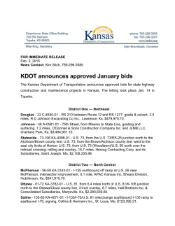

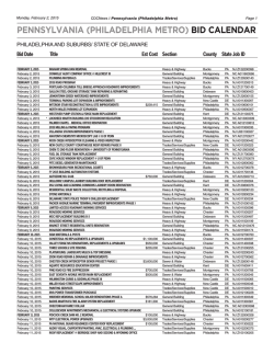

© Copyright 2026